Embed Size (px)
Citation preview
ELSEVIER Parallel Computing 21(1995) 1783-1805
PARALLEL COMPUTING
The REFINE multiprocessor - theoretical properties and algorithms
Suchendra M. Bhandarkar * , Hamid R. Arabnia
Department of Computer Science, 415 Boyd Graduate Studies Research Center, University of Georgia, Athens, GA 30602- 7404, USA
Received 27 June 1994; revised 12 August 1994,27 February 1995
Abstract
A reconfigurable interconnection network based on a multi-ring architecture called REFINE is described. REFINE embeds a single l-factor of the Boolean hypercube in any given configuration. The mathematical properties of the REFINE topology and the hard- ware for the reconfiguration switch are described. The REFINE topology is scalable in the sense that the number of interprocessor communication links scales linearly with network size whereas the network diameter scales logarithmically with network size. Primitive parallel operations on the REFINE topology are described and analyzed. These primitive operations could be used as building blocks for more complex parallel algorithms. A large class of algorithms for the Boolean n-cube which includes the FFT and the Batcher’s bitonic sort is shown to map efficiently on the REFINE topology. The REFINE multiprocessor is shown to offer a cost-effective alternative to the Boolean n-cube multiprocessor architecture without substantial loss in performance.
Keywords: Interconnection networks; Reconfigurable networks; Parallel processing; Dis- tributed computing
1. Introduction
Inherent limitations on the computational power of conventional uniprocessor architectures has lead to the development of parallel multiprocessor architectures. Several multiprocessor architectures have been proposed in the literature such as, the hypercube [ll, systolic array [21, 2-D mesh [3] and the pyramid [4]. It is
* Corresponding author. Email: [email protected]
0167-8191/95/$09.50 0 1995 Elsevier Science B.V. All rights reserved SSDIO167-8191(95)00032-l
1784 SM. Bhandarkar/ParaNel Computing 21 (1995) 1783-1805
considered desirable for the interconnection network describing the multiprocessor architecture to be symmetric and have a low diameter and for each node in the network to have a low degree of connectivity. For most symmetric network topologies, however, the requirements of low degree of connectivity for each node and low network diameter are often conflicting. Low network diameter entails that each node in the network have a high degree of connectivity resulting in a drastic increase in the number of interprocessor communication links. A low degree of connectivity on the other hand, results in a high network diameter which in turn results in high interprocessor communication overhead and reduced efficiency of parallelism.
Reconfigurable networks attempt to address the aforementioned tradeoff be- tween low network diameter and the need to limit the number of inter-processor communication links. In a reconfigurable network each node has a bounded degree of connectivity but the system is allowed to reconfigure itself into different configurations. Examples of reconfigurable multiprocessor systems include the Polymorphic Torus [5], Gated-Connection Network (GCN) [6], CLIP7 [7], PAPIA2 [8l and the reconfigurable bus architecture [9]. Broadly speaking, a reconfigurable system needs to satisfy the following properties in order to be considered practi- cally feasible:
(i) In each configuration the nodes in the network should have a low degree of connectivity with respect to the network size. This is to ensure that the number of interprocessor communication links does not grow rapidly with respect to the network size.
(ii) The network should have a low diameter with respect to the network size. (iii) The algorithmic complexity of reconfiguration with respect to the network size
should be low. (iv) The hardware for the reconfiguration mechanism (i.e. switch) should be of
reasonable complexity with respect to the network size. A simple ring network with N processors has a O(N) diameter and O(N)
number of interprocessor communication links. In fact, the ring network can be shown to be more cost effective [lo] in terms of the number of inter-processor communication links than other interconnection networks such as the systolic array, pyramid or hypercube. The fully connected network with N processors has a O(1) diameter but 0(N2) number of interprocessor communication links, making it very efficient but extremely costly. The hypercube network with N processors has a O(log,N) diameter and O(Nlog,N) number of interprocessor communica- tion links and represents a compromise between the ring and the fully connected network in terms of cost vs. performance. However, it is generally the case that not all the interprocessor communication links in the hypercube are used at the same time during the execution of a parallel program. In fact, there exists a large class of algorithms that uses only the inter-processor communication links along a particu- lar dimension of hypercube at any given time thus resulting in under-utilization of the capabilities of the hypercube topology. This is particularly true of algorithms that use the hypercube in Single Instruction Multiple Data (SIMD) mode or Single Program Multiple Data (SPMD) mode of parallelism.
S.M. Bhandarkar / Parallel Computing 21 (1995) 1783-1805 1785
Blelloch [ll-131 and Little et al. [14&S] have presented a class of SIMD algorithms for the Connection Machine CM-2 (which is an SIMD machine with hypercube topology) based on primitive parallel operations called SCUIZS. Ranka and Sahni [16,17], Lin and Kumar [18], Kumar and Krishnan 1191 and Fang et al. [20] have presented a wide variety of algorithms on the SIMD hypercube for image processing and pattern recognition applications. All these algorithms use only the interprocessor communication links along a particular dimension of hypercube at any given time. Even the algorithms designed by Ranka and Sahni [21,22] and Cypher et al. [23] for the MIMD hypercube, in reality, use the hypercube in SPMD mode since an identical procedure is run on all the node processors of the hypercube. Even in the SPMD mode, only the inter-processor communication links along a particular dimension of hypercube are used at any given time.
In this paper, a reconfigurable interconnection network based on a multi-ring topology is described. The network is shown to have a diameter that scales as O(log, N) and interprocessor communication links that scale as O(N) thus combining the best of the ring and the hypercube network topologies. The network is shown to embed a single l-factor (i.e. interprocessor communication links along a single dimension) of the Boolean hypercube [I] in any given configuration. This network is termed as a REconfigurable l-Factor Hypercubic Embedding Intercon- nection NEtwork (REFINE). The mathematical properties of the interconnection network and the hardware for the reconfiguration switch are described. The hardware for the reconfiguration switch is shown to be scalable with respect to the number of processors in the network. A broad class of algorithms for the Boolean n-cube (hypercube with 2” processors) is shown to map to the REFINE topology in a simple and elegant manner. A variety of parallel procedural primitives for the REFINE multiprocessor are designed and analyzed. These primitives could be used as building blocks for more complex parallel operations. It is shown that the REFINE multiprocessor can be used very effectively in both, tl SIMD and the SPMD modes of parallelism. It is also shown that the REFINE multiprocessor provides the same generality in practice as the n-cube but with far greater cost-effectiveness in terms of hardware complexity and scalability.
2. The basic structure of the REFINE multiprocessor
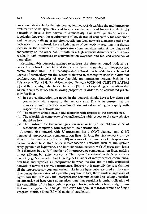
Let RF, denote a REFINE multiprocessor with N = 2” processors. The proces- sors are numbered 0, 1, 2,. . . , N - 1. Each processor p in the the REFINE multiprocessor is uniquely specified using an n bit address (p, _ 1, pn_*, . . . p,J The system RF,, has n + 1 different configurations where each configuration is denoted by config(RF,, i) where 0 I i I n. Let r = 2’, then confg(RF,, i) consists of r = 2’ rings R,, R,, . . . , R,_, such that each ring has k = 2”-’ processors. Fig. l(a) shows the system RF, in configuration config(RF,, 1) whereas Fig. l(b) shows the system RF, in configuration confg(ru;4, 2).
Given that the REFINE multiprocessor is in configuration confg(RF,, i), a processor p is in ring Rj iff p mod r = j. Also, processor p is in position q in the
1786 S.M. Bhundarkar / Parallel Computing 21 (1995) 1783-1805
12
(a)
Fig. 1. RF, in configurations 1 and 2.
ring Rj iff p div r = q. Moreover, processor p is connected to processors ((p + r)mod N) and ((p - rhnod N) in ring Rj via bidirectional channels. As a concrete example, consider the system RF, with N = 24 = 16 processors in config(RF,, 2) i.e. r = 22 = 4. Then, as shown in Fig. l(b):
R, = 0,4,8,12
R, = 1,5,9,13
R, = 2,6,10,14
R, = 3,7,11,15
2.1. The switching network for the REFINE multiprocessor
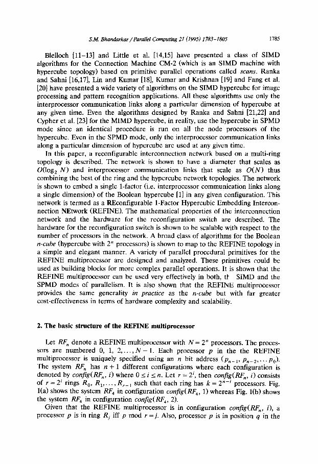
A reconfigurable switch enables the REFINE multiprocessor to reconfigure itself from config(RF,, i) to config@& j) where 0 pi, j sn and i # j. In config(RF,,, i), processor p must be connected to a switch which can connect it to (p + 2’)mod N and (p - 2’)mod N. The function that the switching network needs to perform is related to that of a perfect shuffle network [241 and the barrel shifting network [25], but it is not identical to either of them. As will be shown, the switching network is a subset of the hypercube (i.e. n-cube) network.
Fig. 2. The switch SRI.
S.M. Bhamiarkar /Parallel Computing 21 (1995) 1783-1805 1787
Ao AI X Ao A
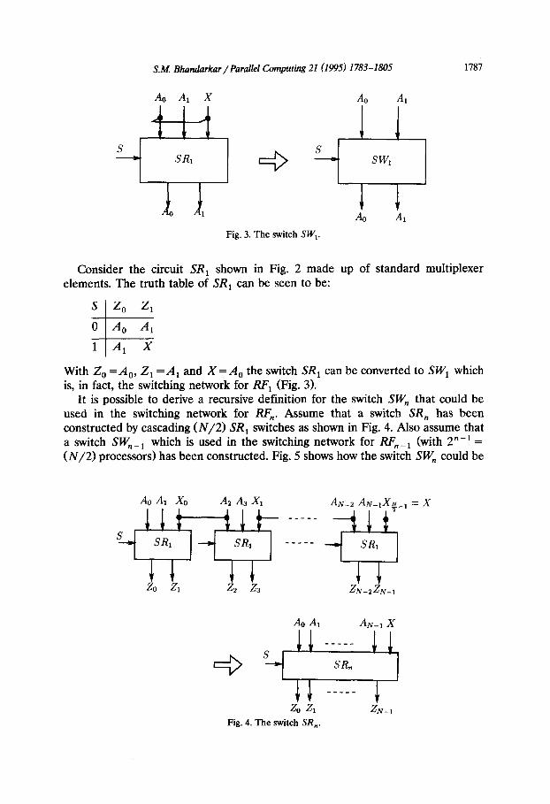
Fig. 3. The switch SW,.
Consider the circuit SR, shown in Fig. 2 made up of standard multiplexer elements. The truth table of SR, can be seen to be:
S Z, Z,
t
0 &I A1
1 A, x
With Z, =A,, Z, =A, and X=A, the switch SR, can be converted to SW, which is, in fact, the switching network for RF, (Fig. 3).
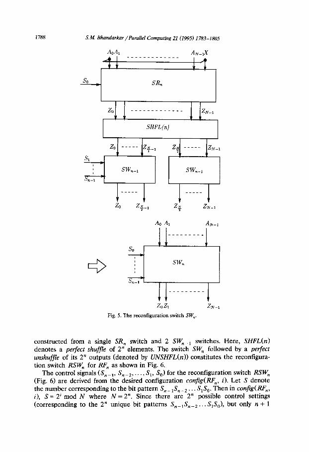
It is possible to derive a recursive definition for the switch SW, that could be used in the switching network for RF,. Assume that a switch SR, has been constructed by cascading (N/2) SR, switches as shown in Fig. 4. Also assume that a switch SW,_ 1 which is used in the switching network for RF,_, (with 2”-’ = (N/2) processors) has been constructed. Fig. 5 shows how the switch SW, could be
ZN-ZZN-,
Ao AI AN-I x
Fig. 4. The switch SR,.
1788 S.M. Bhandarkar /Parallel Computing 21 (1995) 1783-1805
AoA, AN-IX AI
_---___-----_
SHFL (n)
zo Z+, ZN T
ZN-1
Ao A, AN-I
---___--_ v
zo z, ZN-1
Fig. 5. The reconfiguration switch SW,.
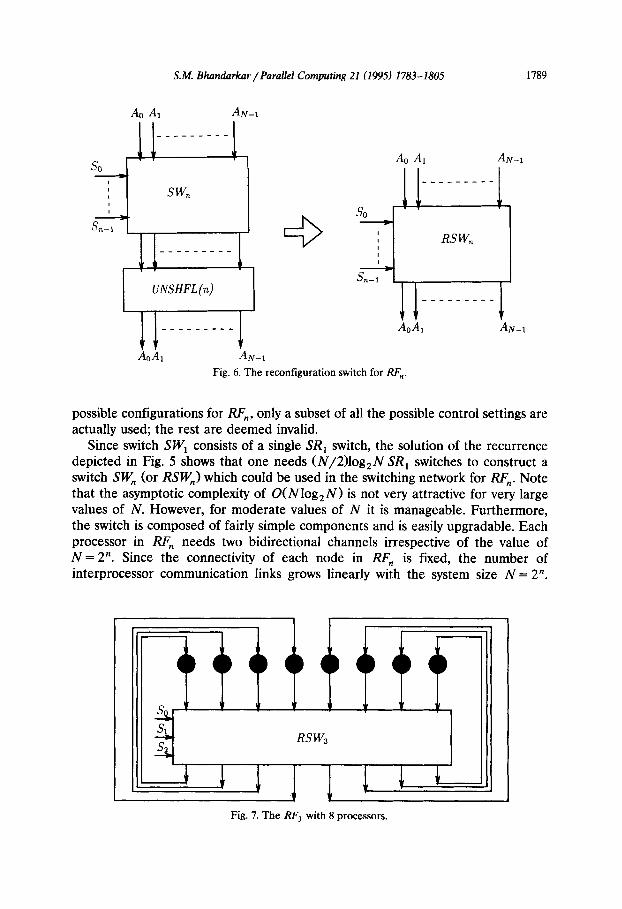
constructed from a single SR, switch and 2 SW,_, switches. Here, SHFL(n) denotes a perfect shuffle of 2” elements. The switch SW, followed by a perfect unshufj?e of its 2” outputs (denoted by UNSHFL(n)) constitutes the reconfigura- tion switch RSW, for RF, as shown in Fig. 6.
The control signals (S, _ r, S, _ 2, . . . , S,, S,) for the reconfiguration switch RSW, (Fig. 6) are derived from the desired configuration config(RF,, 8. Let S denote the number corresponding to the bit pattern S,_ 1Sn_2.. . S,S,. Then in config(RF,, i), S = 2’ mod N where N = 2”. Since there are 2” possible control settings (corresponding to the 2” unique bit patterns S,_,S,_, , . . S,S,), but only n + 1
S.M. Bhandarkar /Par&l Computing 21 (1995) 1783-1805 1789
Ao AI AN-I
___------
so Ao AI AN-I
I __---_---
,
I
I d c so
Y_ I
-.
S-1 I
I RSW,, I __-----_- I
UNSHFL (n) ____--- --
______--- Ao.4
Ao.4 AN-I
Fig. 6. The reconfiguration switch for RF,.
AN-I
possible configurations for RF,, only a subset of all the possible control settings are actually used; the rest are deemed invalid.
Since switch SW, consists of a single SR, switch, the solution of the recurrence depicted in Fig. 5 shows that one needs (N/2)log,N SR, switches to construct a switch SW, (or RSWJ which could be used in the switching network for RF,. Note that the asymptotic complexity of O(Nlog,N) is not very attractive for very large values of N. However, for moderate values of N it is manageable. Furthermore, the switch is composed of fairly simple components and is easily upgradable. Each processor in RF, needs two bidirectional channels irrespective of the value of N = 2”. Since the connectivity of each node in RF, is fixed, the number of inter-processor communication links grows linearly with the system size N = 2”.
Fig. 7. The RF, with 8 processors.
S.M. Bhandarkar /Parallel Computing 21 (1995) 1783-1805
AFAE AD& ABAA AA6
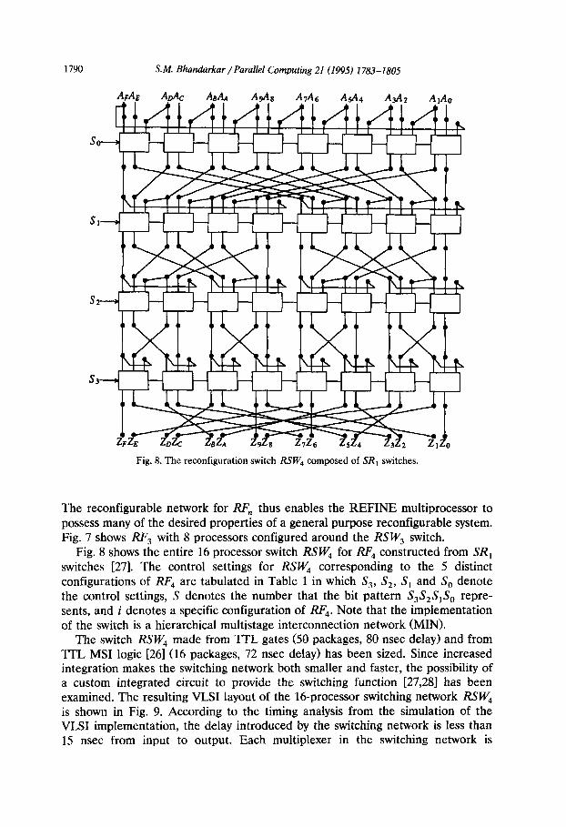
Fig. 8. The reconfiguration switch RSW, composed of SR, switches.
The reconfigurable network for RF, thus enables the REFINE multiprocessor to possess many of the desired properties of a general purpose reconfigurable system. Fig. 7 shows RF, with 8 processors configured around the RSW, switch.
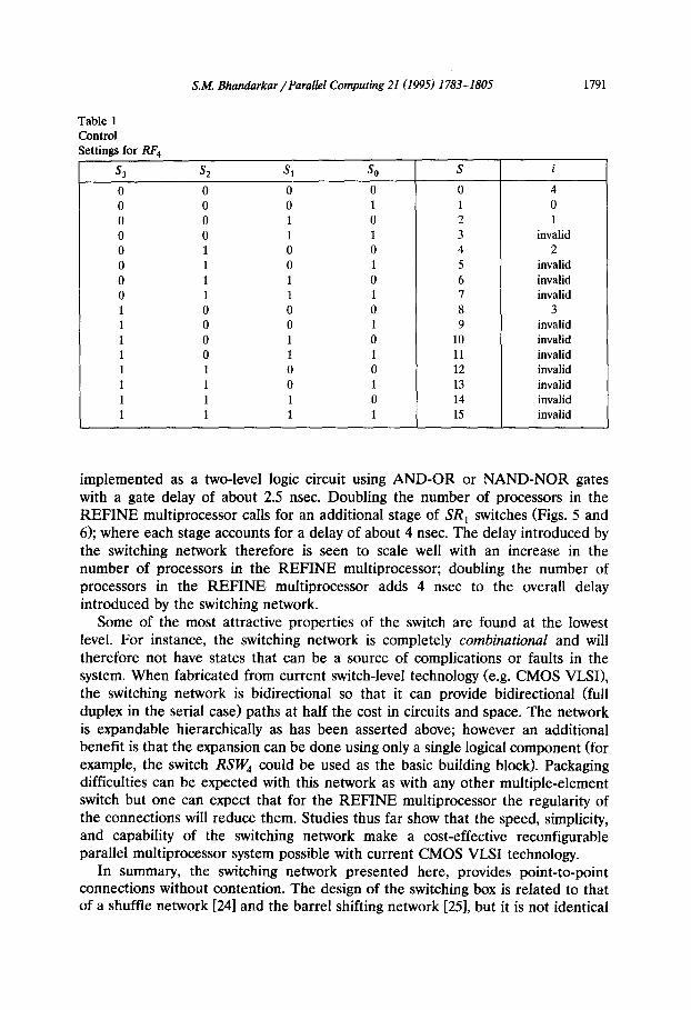
Fig. 8 shows the entire 16 processor switch RSW, for ZW4 constructed from SR, switches [27]. The control settings for RSW, corresponding to the 5 distinct configurations of RF, are tabulated in Table 1 in which S,, S,, S, and S, denote the control settings, S denotes the number that the bit pattern S,S,S,S, repre- sents, and i denotes a specific configuration of RF,. Note that the implementation of the switch is a hierarchical multistage interconnection network (MINI.
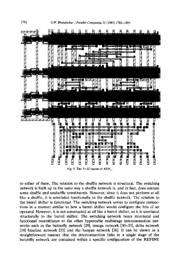
The switch RSW, made from TI’L gates (50 packages, 80 nsec delay) and from TTL MS1 logic [26] (16 packages, 72 nsec delay) has been sized. Since increased integration makes the switching network both smaller and faster, the possibility of a custom integrated circuit to provide the switching function [27,28] has been examined. The resulting VLSI layout of the 16-processor switching network RSW, is shown in Fig. 9. According to the timing analysis from the simulation of the VLSI implementation, the delay introduced by the switching network is less than 15 nsec from input to output. Each multiplexer in the switching network is
S.M. Bhandarkar / Paralkl Computing 21 (1995) 1783-1805 1791
Table 1 Control Settings for RF, -
s3 S2 Sl so
0 0 0 0 0 0 0 1 0 0 1 0 0 0 1 1 0 1 0 0 0 1 0 1 0 1 1 0 0 1 1 1 1 0 0 0 1 0 0 1 1 0 1 0 1 0 1 1 1 1 0 0 1 1 0 1 1 1 1 0 1 1 1 1
S i
0 4 1 0 2 1 3 invalid 4 2 5 invalid 6 invalid 7 invalid 8 3 9 invalid
10 invalid 11 invalid 12 invalid 13 invalid 14 invalid 15 invalid
implemented as a two-level logic circuit using AND-OR or NAND-NOR gates with a gate delay of about 2.5 nsec. Doubling the number of processors in the REFINE multiprocessor calls for an additional stage of SR, switches (Figs. 5 and 6); where each stage accounts for a delay of about 4 nsec. The delay introduced by the switching network therefore is seen to scale well with an increase in the number of processors in the REFINE multiprocessor; doubling the number of processors in the REFINE multiprocessor adds 4 nsec to the overall delay introduced by the switching network.
Some of the most attractive properties of the switch are found at the lowest level. For instance, the switching network is completely combinational and will therefore not have states that can be a source of complications or faults in the system. When fabricated from current switch-level technology (e.g. CMOS VLSI), the switching network is bidirectional so that it can provide bidirectional (full duplex in the serial case) paths at half the cost in circuits and space. The network is expandable hierarchically as has been asserted above; however an additional benefit is that the expansion can be done using only a single logical component (for example, the switch RSW, could be used as the basic building block). Packaging difficulties can be expected with this network as with any other multiple-element switch but one can expect that for the REFINE multiprocessor the regularity of the connections will reduce them. Studies thus far show that the speed, simplicity, and capability of the switching network make a cost-effective reconfigurable parallel multiprocessor system possible with current CMOS VLSI technology.
In summary, the switching network presented here, provides point-to-point connections without contention. The design of the switching box is related to that of a shuffle network 1241 and the barrel shifting network [25], but it is not identical
1792 S.M. Bhandarkar / Parallel Computing 21 (1995) 1783-1805
Fig. 9. The VLSI layout of RSW,.
to either of them. The relation to the shuffle network is structural. The switching network is built up in the same way a shuffle network is, and in fact, does contain some shuffle and unshuffle constituents. However, since it does not perform at all like a shuffle, it is unrelated functionally to the shuffle network. The relation to the barrel shifter is functional. The switching network serves to configure connec- tions in a manner similar to how a barrel shifter would configure the bits of an operand. However, it is not constructed at all like a barrel shifter, so it is unrelated structurally to the barrel shifter. The switching network bears structural and functional resemblance to the other hypercubic multistage interconnection net- works such as the butterfly network [29], omega network [30-331, delta network [34] baseline network 1351 and the banyan network [361. It can be shown in a straightforward manner that the interconnection links in a single stage of the butterfly network are contained within a specific configuration of the REFINE
S.M. Bhandarkar /Parallel Computing 21 (1995) 1783-1805 1793
topology. This property can be proved in a manner analogous to the proof of Theorem 3.1. Leighton [37] has shown the other commonly encountered multistage interconnection networks, i.e. omega, baseline, delta and banyan, to be variants of the butterfly network. In [37] Leighton has presented a class of graph similarity transformations for systematically transforming the other networks into an equiva- lent representation in terms of the butterfly network. This implies that the various stages of the omega, baseline, delta and banyan networks can also be shown to be contained within specific configurations of the REFINE topology.
3. Basic properties of the REFINE multiprocessor
In this section some important properties of the REFINE multiprocessor are stated and proved. These properties provide the basis for the parallel procedural primitives presented in the following section.
3.1. The REFINE multiprocessor and the n-cube
An interconnection network can be looked upon as a graph G(V, E) with the processing elements comprising the set of vertices I/ and the communication links between the processing elements comprising the set of edges E. A set of edges in G is said to be disjoint if no two edges in the set share a common vertex. A l-factor F of G is a set of disjoint edges such that each vertex in G lies on one and only one edge in F. A set of edge-disjoint l-factors F,, F,, . . . , F,_, such that F, u F1 . . . u F,_, = E constitutes a l-factorization of the graph G. The n-cube has a l-factorization consisting of n sets of parallel edges in each of the dimensions [38]. The REFINE multiprocessor RF,, will be shown to be very closely related to the well researched n-cube multiprocessor.
Theorem 3.1. The REFINE multiprocessor RF, in a given configuration embeds a single l-factor of the n-cube.
Proof. Let 4” be the collection of edges in the n-cube in the ith dimension, i.e. E;;” = {(p, q)} such that the binary addresses of processors p and q differ in only the ith bit. Then F,“, F,“, . . . , F,“_, represents a l-factorization of the n-cube. Note that if the processors p and q are directly connected to each other in the n-cube then their addresses differ only in the ith bit for some i such that 0 pi sn - 1.
Without loss of generality, one may assume that the ith bit of p = 0 and the ith bit of q = 1. Therefore q =p -t 2’ and from the definition of confg(W,, i) given in Section 2 p and q are connected in confg(RF,, i) i.e. FF cconfg(W,, i). Thus config(R&, i) of the REFINE multiprocessor embeds the l-factor Fj” of the n-cube. III
There exists a large class of algorithms for the n-cube that at any given time uses only the edges in Fin for some i, i.e. communication is done along a particular
1794 S.M. Bhandarkar /Parallel Computing 21 (1995) 1783-1805
dimension of the n-cube at any given time. This is particularly true of algorithms that use the n-cube in the SIMD or SPMD modes of parallelism. As can be deduced from Theorem 3.1, such algorithms for the n-cube can be easily mapped onto the REFINE topology without loss of performance assuming that the over- head in reconfiguration is not excessive. This leads to the following corollary:
Corollary 3.1. Any algorithm which uses the communication links along a single dimension of the n-cube at any given point in time can be mapped to the REFINE multiprocessor RF, in O(1) time.
Proof. Let p(i) represent the processor whose n bit address differs from that of processor p only in the ith bit. Let p[i] denote the ith bit in the n bit address of processor p. Let A(p) denote the A register in processor p. Let the statement reconfg(n, i) reconfigure RF, in config(RF,, i). Also, let left(p) and right(p) denote the processors (p - 2’hrod N and (p + 2’knod N in config(RF,, i). Each statement A(p) --, A(p(i)) in an algorithm for the n-cube which moves the contents of the A register of p to the A register of p(i) along the edge (p, p(i)) in the ith dimension is equivalent to
reconfigcn, i);
IF (pCil=O) THEN A(p)-+A(right(p))
ELSE A(p) -+A(left(p));
for the REFINE multiprocessor RF,, with N = 2” processors. Similarly, every statement A(p) + A(p(i)) in an algorithm for the n-cube is equivalent to
reconfigcn, i);
IF (pCil=O) THEN A(p)tA(right(p))
ELSE A(p) +A(left(p));
It is therefore obvious that any algorithm which uses the communication links along a single dimension of the n-cube at any given point in time can be mapped to the REFINE multiprocessor RF, in O(1) time. 0
3.2. Subconfigurations of the REFINE topology
One of the attractive features of the n-cube is that its structure has a simple recursive property. An n-cube can be looked upon as a. l-cube composed of two (n - I)-cubes or a 2-c&e composed of four (n - 2)-cubes and so on. In general, an n-cube can be looked upon as an m-cube of 2” nodes, each node of which is in turn a (n - ml-cube where m < n. In this case the binary address p of a processor in the n-cube can be decomposed as p =pmpn_,,, where the higher order pm bits specify the node (i.e. the (n - m&cube) within the m-cube and the lower-order p,,_,,, bits specify the node within the (n - m)-cube. This simple recursive property
SM. Bhundarkar / Parallel Computing 21 (1995) 1783-1805 1795
of the n-cube has been exploited by several researchers in designing elegant and efficient algorithms for the n-cube.
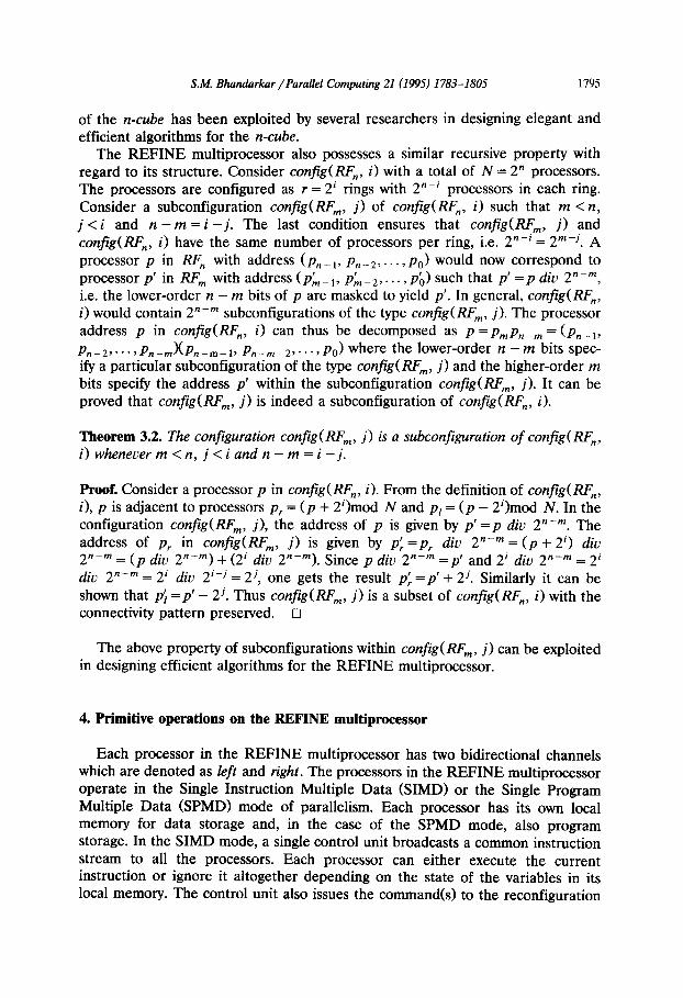
The REFINE multiprocessor also possesses a similar recursive property with regard to its structure. Consider config(RF,, i) with a total of N = 2” processors. The processors are configured as r = 2’ rings with 2”-’ processors in each ring. Consider a subconfiguration config(RF,, j) of config(RF,, i) such that m <n, j < i and n -m = i - j. The last condition ensures that config(H$,, j) and config(RF,, i) have the same number of processors per ring, i.e. 2”-’ = 2”-j. A processor p in RF,, with address (p,_ ,, P”_~, . . . , pO) would now correspond to processor p’ in RF, with address <pk_,, PL_~, . . . , pb) such that p’ =p div 2”-“, i.e. the lower-order IZ - m bits of p are masked to yield p’. In general, confg(RF,, i) would contain 2”-” subconfigurations of the type config@&, j). The processor address p in config(RF,,, i) can thus be decomposed as p =pmpn_,,, = (p,_ 1,
P,- 29 * * * 7 Pn-mXPn-m-l, Pn-m-2,. * 1, pO> where the lower-order IZ - m bits spec- ify a particular subconfiguration of the type config( RF’, j) and the higher-order m bits specify the address p’ within the subconfiguration co@g(RF,, j). It can be proved that config(RF,, j) is indeed a subconfiguration of config(RF,, i).
Theorem 3.2. The configuration config(R&, j) is a subconfiguration of config(m,, i)wheneverm<n, j<iandn-m=i-j.
Proof. Consider a processor p in config(RF,, i). From the definition of config(RF,, i), p is adjacent to processors p, = (p + 2’)mod N and p, = (p - 2’)mod N. In the configuration co@g(RF,, j), the address of p is given by p’ =p div 2”-“. The address of pr in config(RF,, j) is given by pi =p, div 2”-” = (p + 29 div 2”-” = (p div 2 ‘-“‘) + (2’ div 2”-,). Since p div 2”-” =p’ and 2’ div 2”-” = 2’ div 2”-” = 2’ div 2’-’ = 2j, one gets the result p: =p’ + 2’. Similarly it can be shown that pi =p’ - 2’. Thus config(RF,, j) is a subset of confg(lW,, i) with the connectivity pattern preserved. 0
The above property of subconfigurations within config(RF,, j) can be exploited in designing efficient algorithms for the REFINE multiprocessor.
4. Primitive operations on the REFINE multiprocessor
Each processor in the REFINE multiprocessor has two bidirectional channels which are denoted as Zeft and right. The processors in the REFINE multiprocessor operate in the Single Instruction Multiple Data (SIMD) or the Single Program Multiple Data (SPMD) mode of parallelism. Each processor has its own local memory for data storage and, in the case of the SPMD mode, also program storage. In the SIMD mode, a single control unit broadcasts a common instruction stream to all the processors. Each processor can either execute the current instruction or ignore it altogether depending on the state of the variables in its local memory. The control unit also issues the command(s) to the reconfiguration
1796 S.M. Bhandarkar /Parallel Computing 21 (1995) 1783-1805
switch to reconfigure the REFINE multiprocessor in a given configuration. In the SIMD mode all the processors and the reconfiguration switch are constrained to operate in lockstep synchronism. In the SPMD mode of parallelism each processor runs its local program asynchronously on its local data. However, all the processors are synchronized at each reconfigure command using barrier synchronization. A failure to do so would cause an inconsistency if different processors assume different states of the interconnection network and also contention at the switch level if the switch is forced to route messages in two different reconfiguration states at the same time.
The following conventions are used in algorithms designed for the REFINE multiprocessor:
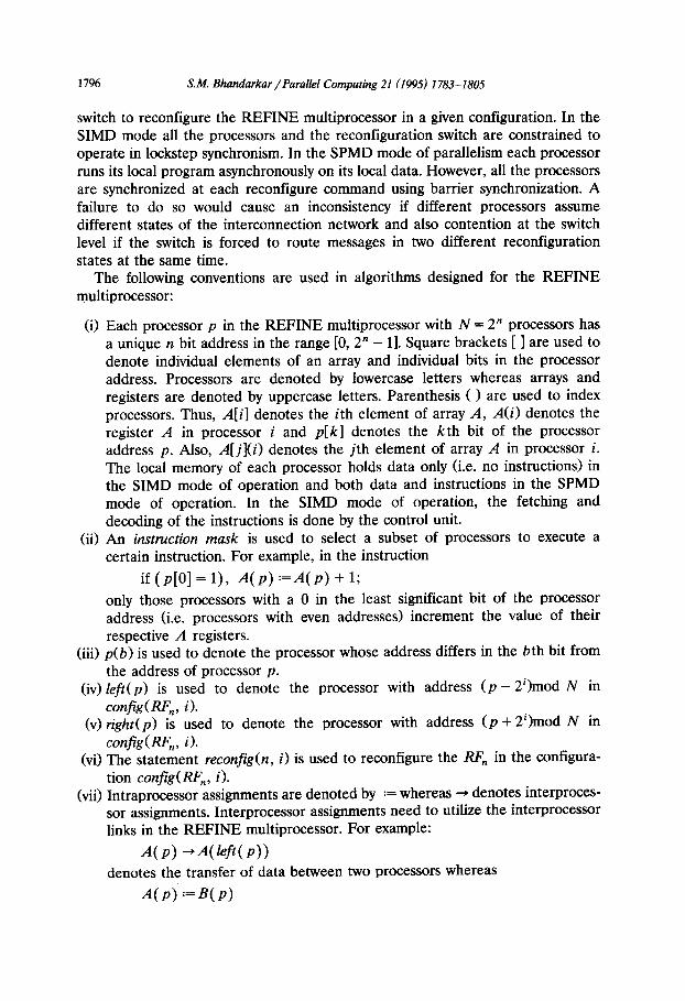
(i) Each processor p in the REFINE multiprocessor with N = 2” processors has a unique IZ bit address in the range [0, 2” - 11. Square brackets [ ] are used to denote individual elements of an array and individual bits in the processor address. Processors are denoted by lowercase letters whereas arrays and registers are denoted by uppercase letters. Parenthesis ( ) are used to index processors. Thus, A[i] denotes the ith element of array A, A(i) denotes the register A in processor i and p[ k] denotes the kth bit of the processor address p. Also, A[ j](i) denotes the jth element of array A in processor i. The local memory of each processor holds data only (i.e. no instructions) in the SIMD mode of operation and both data and instructions in the SPMD mode of operation. In the SIMD mode of operation, the fetching and decoding of the instructions is done by the control unit.
(ii) An instruction mask is used to select a subset of processors to execute a certain instruction. For example, in the instruction
if (p[O] = l), A(p) :=A( p) + 1;
only those processors with a 0 in the least significant bit of the processor address (i.e. processors with even addresses) increment the value of their respective A registers.
(iii) p(b) is used to denote the processor whose address differs in the bth bit from the address of processor p.
(iv) left(p) is used to denote the processor with address (p - 2’)mod N in config(zW,, i).
(v) right(p) is used to denote the processor with address (p + 2’)mod N in confg(RF,, i).
(vi) The statement reconfig(n, i) is used to reconfigure the RF, in the configura- tion config(RF,, il.
(vii) Intraprocessor assignments are denoted by := whereas + denotes interproces- sor assignments. Interprocessor assignments need to utilize the inter-processor links in the REFINE multiprocessor. For example:
4 P) -Weft(p)) denotes the transfer of data between two processors whereas
A(P) :=B(p)
S.M. Bhandarkar /ParaNel Computing 21 (1995) 1783-1805 1797
Broadcast(X, n); BEGIN
FOR i = 0 to n-l DO
BECINFOR reconfigb, i);
IF (WSONE(p) = i) THEN X(p) <-- X(left(p));
ENDFOR;
END;
Fig. lO.Broadcast operation.
denotes an intraprocessor assignment. The term unit hop is used to denote communication between processors in the REFINE multiprocessor that are directly connected. The asymptotic complexity of an algorithm for the RE- FINE multiprocessor is decided by the number of unit hops in the algorithm.
5. Algorithms for the REFINE multiprocessor
In this section the implementation of some algorithms on the REFINE multi- processor is considered.
5.1. Basic message passing operations
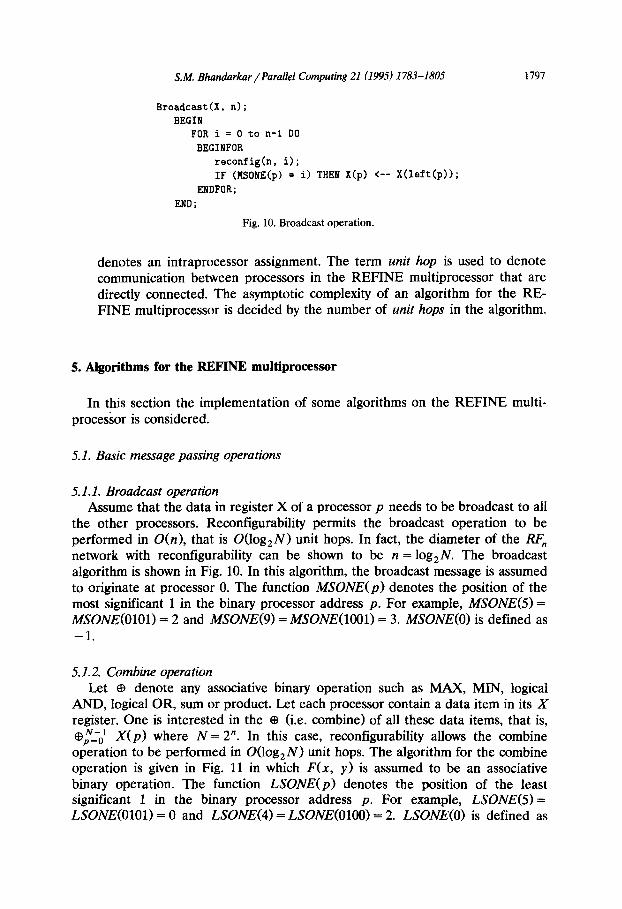
5.1.1. Broadcast operation Assume that the data in register X of a processor p needs to be broadcast to all
the other processors. Reconfigurability permits the broadcast operation to be performed in O(n), that is O(log,N) unit hops. In fact, the diameter of the RF, network with reconfigurability can be shown to be n = log,N. The broadcast algorithm is shown in Fig. 10. In this algorithm, the broadcast message is assumed to originate at processor 0. The function MSONE(p) denotes the position of the most significant 1 in the binary processor address p. For example, MSONE(5) = A4SOZV_E(OlOl) = 2 and MSONE(9) = MSOZV..(lOOl) = 3. MSONE(0) is defined as -1.
5.1.2. Combine operation Let ~3 denote any associative binary operation such as MAX, MIN, logical
AND, logical OR, sum or product. Let each processor contain a data item in its X register. One is interested in the @ (i.e. combine) of all these data items, that is, @F&i X(p) where N = 2”. In this case, reconfigurability allows the combine operation to be performed in O(log,iV) unit hops. The algorithm for the combine operation is given in Fig. 11 in which F(x, y) is assumed to be an associative binary operation. The function LSONE(p) denotes the position of the least significant 1 in the binary processor address p. For example, LSONE(5) = LSONE(O101) = 0 and LSONE(4) = LSONE(O100) = 2. LSONE(0) is defined as
1798 SM. Bhandarkar /Parallel Computing 21 (1995) 1783-1805
Combine(X, n, F); BEGIN
FOR i = 0 to n-l DO BEGINFOR
rsconfig(n.i); IF (LSONE(p) = i) THEN X(p) --> Y(left(p)); IF (p[i] = 0) THEN X(p) := F(X(p),Y(p)); {F is an associative binary operation>
ENDFOB;
END;
Fig. 11. Combine operation.
- 1. At the end of the combine operation processor 0 contains the final result of the combine operation.
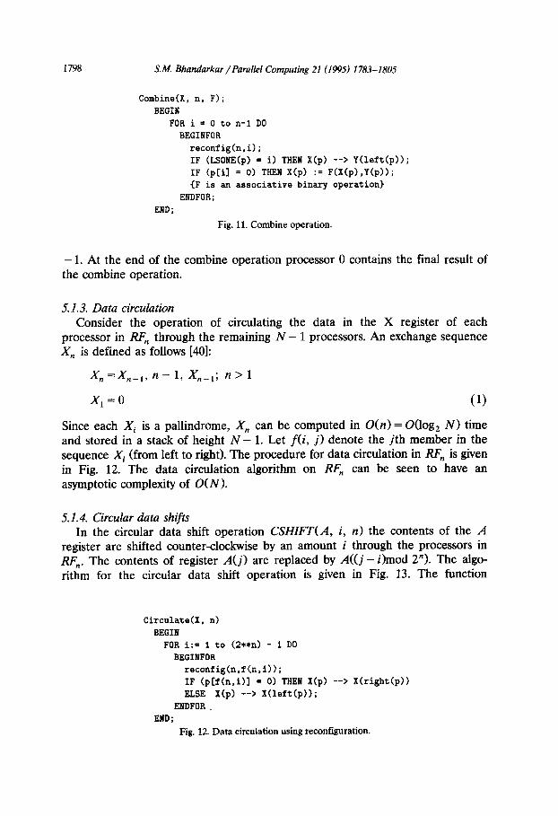
5.1.3, Data circulation Consider the operation of circulating the data in the X register of each
processor in RF, through the remaining N - 1 processors. An exchange sequence X,, is defined as follows [40]:
x, =xn_i, Iz - 1, x,_,; n > 1
xi = 0 (1)
Since each Xi is a pallindrome, X, can be computed in O(n) = O(log, N) time and stored in a stack of height N - 1. Let f(i, j) denote the jth member in the sequence Xi (from left to right). The procedure for data circulation in RF, is given in Fig. 12. The data circulation algorithm on RF, can be seen to have an asymptotic complexity of O(N).
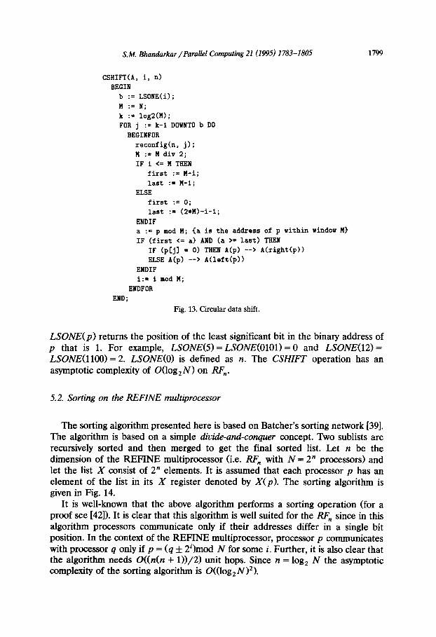
51.4. Circular data shifts In the circular data shift operation CSHIFT(A, i, n) the contents of the A
register are shifted counter-clockwise by an amount i through the processors in RF,. The contents of register A(j) are replaced by A((j - i)mod 2”). The algo- rithm for the circular data shift operation is given in Fig. 13. The function
Circulate(X, n) BEGIN FOR i:= 1 to (2*+n) - 1 DO
BEGINFOR reconfig(n,f(n.i));
IF (pCf(n.i)l = 0) THEN X(p) --> X(right(p)) ELSE X(p) --> X(left(p));
ENDFOR. END;
Fig. 12. Datacirculation using reconfiguration.
SM. Bhandarkar/Parallel Computing 21 (1995) 1783-1805 1799
CSHIFT(A, i, n) BEGIN b := LSONE(i); I4 := N;
k := logTt(M); FOR j := k-l DOUNTO b DO
BEGINFOR reconfig(n. j); M := M div 2; IF i <= M THEN
first := M-i; last := M-l;
ELSE first := 0; last := (l*M)-i-l;
ENDIF a := p mod M; {a is the address of p within windou Ml
IF (first <= a) AND (a >= last) THEN
IF (PO1 = 0) THEN A(p) --> A(right(p)) ELSE A(p) --> A(left(p))
ENDIF i:= i mod M;
ENDFOR END;
Fig. 13. Circular data shift.
LYON,??(p) returns the position of the least significant bit in the binary address of p that is 1. For example, LSONE(5) =LSONE(OlOl) = 0 and LSONE(12) = LSONE(1100) = 2. LYONHO) is defined as n. The CSHZFT operation has an asymptotic complexity of O(log,N) on RF,.
5.2. Sorting on the REFINE multiprocessor
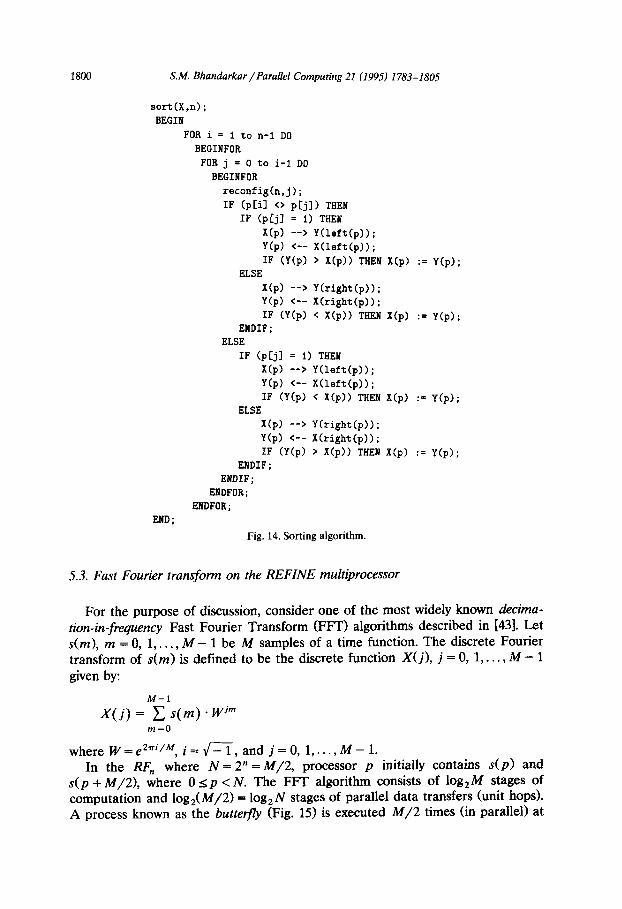
The sorting algorithm presented here is based on Batcher’s sorting network [39]. The algorithm is based on a simple divide-and-conquer concept. Two sublists are recursively sorted and then merged to get the final sorted list. Let n be the dimension of the REFINE multiprocessor (i.e. RF, with N = 2” processors) and let the list X consist of 2” elements. It is assumed that each processor p has an element of the list in its X register denoted by X(p). The sorting algorithm is given in Fig. 14.
It is well-known that the above algorithm performs a sorting operation (for a proof see [42]). It is clear that this algorithm is well suited for the RF, since in this algorithm processors communicate only if their addresses differ in a single bit position. In the context of the REFINE multiprocessor, processor p communicates with processor q only if p = (q f 2’)mod N for some i. Further, it is also clear that the algorithm needs O((n(n + 1))/2) unit hops. Since n = log, N the asymptotic complexity of the sorting algorithm is 0((log,Nj2).
1800 S.M. Bhndarkar/Parallel Computing 21 (1995) 1783-1805
sort(X,n); BEGIN
FOR i = 1 to n-l DO BEGINFOR FOR j = 0 to i-i DO BEGINFOR
reconfigcn, j) ; IF (pcil <> p[jl) THEN
IF (pCj1 = 1) THEN X(p) --> Y(left(p)); Y(p) <-- X(left (p) 1; IF (Y(p) > X(p)) THEN X(p) := Y(p);
ELSE
X(p) --> Y(right(p)); Y(p) <-- X(right(p)); IF (Y(p) < X(p)) THEN
ENDIF; ELSE
IF (pCj1 = 1) THEN
X(p) --> Y(left(p)); Y(p) <-- X(left (p) 1; IF (Y(p) < X(p)) THEN
ELSE X(p) --> Ykight (p) 1; Y(p) <-- X(right(p)); IF (Y(p) > X(p)) THEN
ENDIF; ENDIF;
ENDFOR; ENDFOR;
X(p) := Y(p);
X(p) := Y(p);
X(p) := Y(p);
Fig. 14. Sorting algorithm.
5.3. Fast Fourier transform on the REFINE multiprocessor
For the purpose of discussion, consider one of the most widely known decima- tion-in-frequency Fast Fourier Transform (FFT) algorithms described in [43]. Let s(m), m = 0, 1,. . . , A4 - 1 be M samples of a time function. The discrete Fourier transform of s(m) is defined to be the discrete function X( j>, j = 0, 1,. . . , M - 1 given by:
M-l
X(j) = C s(m) * Wj” m=O
where W- e2Ti/M, i = m, and j = 0, 1,. . . , A4 - 1. In the RF,, where N = 2 n = M/2, processor p initially contains s(p) and
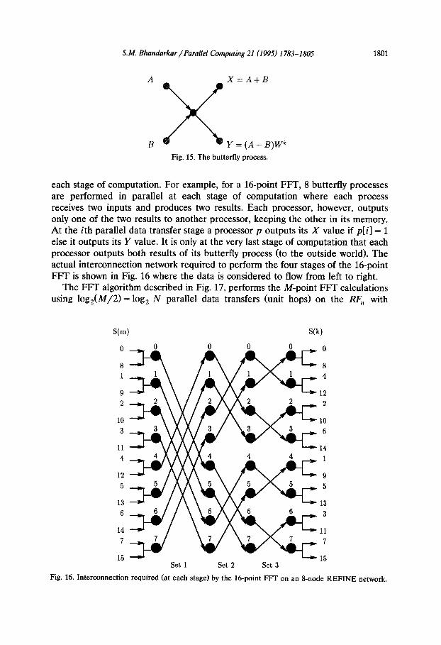
S( p + M/2), where 0 sp < N. The Fm algorithm consists of log,M stages of computation and log,(M/2) = log,N stages of parallel data transfers (unit hops). A process known as the butterfry (Fig. 15) is executed M/2 times (in parallel) at
S.M. Bhandarkar / Parallel Computing 21 (1995) 1783-1805 1801
A X=A+B
B Y=(A-B)Wk
Fig. 15. The butterfly process.
each stage of computation. For example, for a 16point FFT, 8 butterfly processes are performed in parallel at each stage of computation where each process receives two inputs and produces two results. Each processor, however, outputs only one of the two results to another processor, keeping the other in its memory. At the ith parallel data transfer stage a processor p outputs its X value if p[i] = 1 else it outputs its Y value. It is only at the very last stage of computation that each processor outputs both results of its butterfly process (to the outside world). The actual interconnection network required to perform the four stages of the 16-point FIT is shown in Fig. 16 where the data is considered to flow from left to right.
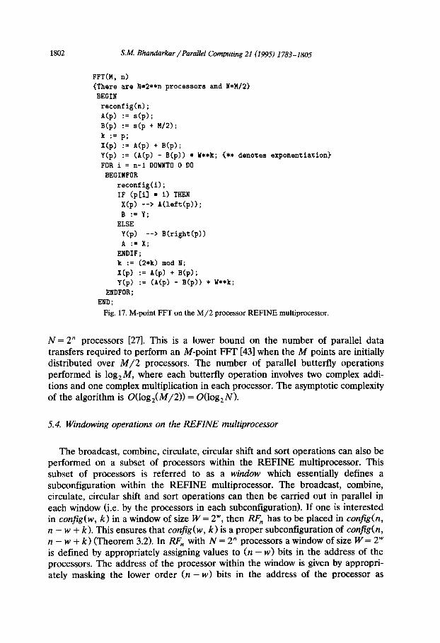
The FFT algorithm described in Fig. 17, performs the M-point FFT calculations using log,(M/2) = log, N parallel data transfers (unit hops) on the RF,, with
S(m) S(k)
Fig. 16.
Set 1 Set 2 Set 3
Interconnection required (at each stage) by the 16-point FFT on an I-node R .EFINE network.
1802 S.M. Bhandarkar / Parallel Computing 21 (1995) 1783-1805
FFT(H, n) {There are N=2**n processors and N=M/2)
BEGIN
reconfig(n);
A(p) := s(p);
B(p) := s(p + M/2);
k := Pi X(p) := A(p) + B(p);
Y(p) := (A(p) - B(p)) * U**k; (** denotes exponentiation)
FOR i = n-l DOWNTO 0 DO
BECINFOR reconfig(i);
IF (pi3 = 1) THEN
X(p) --> A(left(p)); B := Y.
ELSE
Y(p) --> B(right(p)) A .= X. . , ENDIF; k := (2*k) mod N;
X(p) := A(p) + B(p);
Y(p) := (A(p) - B(p)) * W**k;
ENDFOR; END;
Fig.17.M-point FFTonthe M/2processor REFINEmultiprocessor.
N = 2” processors [27]. This is a lower bound on the number of parallel data transfers required to perform an M-point FFT [43] when the M points are initially distributed over M/2 processors. The number of parallel butterfly operations performed is log,M, where each butterfly operation involves two complex addi- tions and one complex multiplication in each processor. The asymptotic complexity of the algorithm is O(log,(M/2)) = O(log,N).
5.4. Windowing operations on the REFINE multiprocessor
The broadcast, combine, circulate, circular shift and sort operations can also be performed on a subset of processors within the REFINE multiprocessor. This subset of processors is referred to as a window which essentially defines a subconfiguration within the REFINE multiprocessor. The broadcast, combine, circulate, circular shift and sort operations can then be carried out in parallel in each window (i.e. by the processors in each subconfiguration). If one is interested in config(w, k) in a window of size W = 2”, then RF,, has to be placed in config(n, n - w + k). This ensures that confg(w, k) is a proper subconfiguration of configb, n - w + k) (Theorem 3.2). In RF, with N = 2” processors a window of size W = 2” is defined by appropriately assigning values to (n - w) bits in the address of the processors. The address of the processor within the window is given by appropri- ately masking the lower order (n - w) bits in the address of the processor as
S.M. Bhandarkor /Parallel Computing 21 (1995) 1783-1805 1803
discussed in Section 3.2. It can be seen that the broadcast, combine, circular shift and FFT operations can be performed in O(log,W) unit hops, the circulate operation in O(W) unit hops and the sort operation in O((log,IU2> unit hops in a window of size W = 2”. The algorithms for the broadcast, combine, circulate, circular shift and sort operations within a window are similar to the ones already described and hence will not be repeated here.
6. Conclusions
In this paper, a reconfigurable interconnection network based on a multi-ring topology termed as REFINE was described. The REFINE was shown to embed a single l-factor of the Boolean hypercube in any given configuration. The mathe- matical properties of the interconnection network and the hardware for the reconfiguration switch were described. Since most SIMD and SPMD algorithms for the n-cube exploit only the edges along a given dimension at any point in time, a large class of algorithms for the n-cube which includes the FFT and Batcher’s bitonic sort were shown to map onto the REFINE multiprocessor without loss of performance. The REFINE topology is scalable since the degree of connectivity of each processor is 2 irrespective of the number of processors in the network. This ensures that the number of interprocessor communication links scales linearly with network size. The diameter of the REFINE topology scales as O(log,N) with network size. The REFINE topology was thus seen to combine the advantages of low network diameter coupled with a fixed degree of connectivity for each node in the network. The paper also described primitive parallel operations such as broadcast, combine, circular shift and data circulate on the REFINE multiproces- sor network. These primitive operations could be used as building blocks for more complex parallel algorithms. The proposed interconnection network was shown to offer a cost-effective alternative to the hypercube multiprocessor architecture without substantial loss in performance.
References
[l] M.C. Pease, The indirect binary n-cube microprocessor array, IEEE Trans. Comput. C-25 (5) (1977) 458-473.
[2] H.T. Kung, Why systolic architectures, IEEE Computer 15 (Jan. 1982) 37-46. [3] R. Miller and Q.F. Stout, Geometric algorithms for digitized pictures on a mesh connected
computer, IEEE Trans. Pattern Analysis and Mach. Intell. 7 (2) (March 1985) 216-228. [4] V. Di Gesu, An overview of pyramid architectures for image processing, Information Sciences 47
(1989) 17-34. [5] H. Li and M. Maresca, Polymorphic torus network, IEEE Trans. Computers C-38 (9) (Sep. 1989)
1345-1351. [6] D.B. Shu and J.G. Nash, The gated interconnection network for dynamic programming, in
Concurrent Computations, S.K. Tewsburg et al. (Eds.) (Plenum, New York, 1988). [7] T.J. Fountain and V. Goetcherian, CLIP7 parallel processing system, Proc. IEE, Part E, 127 (5)
(1980) 219-224.
1804 S.M. Bhandarkar/Parallel Compuring 21 (1995) 1783-1805
[Sl V. Cantoni, M. Ferretti, S. Levialdi and R. Stefanelli, PAPIA: Pyramidal Architecture for Parallel Image Analysis, Proc. 7th Symp. Computer Arithmetic, Urbana, IL (1985) 237-242.
[9] R. Miller, V.K. Prasanna Kumar, D. Reiss and Q.F. Stout, Image computations on reconfigurable VLSI arrays, Proc. IEEE Conf: Computer Vision and Pattern Recognition (1988) 925-930.
[lo] A.J. Anderson, Multiple Processing-A Systems Overview (Prentice Hall, 1989). (111 G.E. Blelloch, Vector Models for Data Parallel Compuring (MIT Press, Cambridge, MA, 1990). [12] G.E. Blelloch, Scans as primitive parallel operations, IEEE Trans. Computers 38 (11) (Nov. 1989)
1526-1538. [13] G.E. Blelloch and J.J. Little, Parallel solutions to geometric problems on the scan model of
computation, Proc. Znd. Co@ Parallel Processing 3 (Aug. 1988) 218-222. [14] J.J. Little, G.E. Blelloch and T. Cass, Parallel algorithms for computer vision on the Connection
Machine, Proc. Zntl. Conf Computer tision (June 1987) 587-591. [15] J.J. Little, G.E. Blelloch and T. Cass, Algorithmic techniques for computer vision on a fine-grained
parallel machine, IEEE Trans. Pattern Anal. Mach. Zntell. 11 (3) (March 1989) 244-257. 1161 S. Ranka and S. Sahni, Image template matching on SIMD hypercube multicomputers, Proc. Znrl.
Conf. Parallel Processing (1988) 84-91. [17] S. Ranka and S. Sahni, Odd even shifts in SIMD hypercubes, IEEE Trans. Parallel and Distributed
Systems 1 (1) (Jan. 1990) 77-76. [18] W.M. Lin and V.K.P. Kumar, Efficient histogramming on hypercube SIMD machines, Computer
F&on Graphics Image Proc. 49 (1990) 104-120. [19] V.K.P. Kumar and V. Krishnan, Efficient image template matching on hypercube SIMD arrays,
Proc. Zntl. Conf. Parallel Processing (1987) 765-771. [20] Z. Fang, X. Li and L.M. Ni, Parallel algorithms for image template matching on hypercube SIMD
computers, IEEE Workshop on Camp. Arch. for Pattern Analysis and Image Database Mgmt. (1985) 33-40.
[21] S. Ranka and S. Sahni, Computing Hough transforms on hypercube multicomputers, J. Supercom- puting 4 (1990) 169-190.
[22] S. Ranka and S. Sahni, Image template matching on MIMD hypercube multicomputers, Proc. Znrl. Conf. Parallel Processing (1988) 92-99.
[23] R. Cypher, J.L.C. Sanz and L. Synder, Hypercube and shuffle-exchange algorithms for image component labeling, Proc. IEEE Znd. Wkshp. Comp. Arch. Pattern Anal. Mach. Zntell. (Oct. 1987) 5-10.
[24] H.S. Stone, High Performance Computer Architecture (Addison-Wesley, NY, 1990). [25] C. Mead and L. Conway, VLSI Systems Design (Addison-Wesley, NY, 1980). [26] Texas Instruments, ?TL Logic Data Book (Texas Instruments, 1988). [27] S.M. Bhandarkar, H.R. Arabnia and J.W. Smith, A reconfigurable architecture for image process-
ing and computer vision, Znd. Jour. Pattern Recog. Art. Zntell. 9(2) (April 1995) 201-229. [28] SM. Bhandarkar and H.R. Arabnia, A multi-ring reconfigurable multiprocessor network for
computer vision, Proc. IEEE Znd. Wkshp. on Computer Arch. for Machine Vision, New Orleans, LA (Dec. 1993) 180-190.
[29] BBN Advanced Computers Inc., Cambridge, MA, TC2000 Technical product summary, Nov. 1989. [30] G.F. Pfister and V.A. Norton, Hot spot contention and combining in multistage interconnection
networks, Proc. Zntl. Conf. Parallel Processing (Aug. 1985) 790-797. [31] A. Gottleib, R. Grishman, C.P. Kruskal, K.P. McAuliffe, L. Rudolf and M. Snir, The NYU
ultracomputer-Designing an MIMD shared memory parallel computer, IEEE Trans. Computers 32, (2) (Feb. 1986) 175-189.
[32] D.J. Kuck, E.S. Davidson, D.H. Lawrie and A.H. Sameh, Parallel supercomputing today-The Cedar approach, Science, 231 (2) (Feb. 1986).
[33] D.H. Lawrie, Access and alignment of data in an array processor, IEEE Trans. Computers (Dec. 1975).
[34] J.H. Patel, Performance of processor-memory interconnections for multiprocessors, IEEE Trans. Computers 27 (10) (Oct. 1981) 771-780.
[35] C.L. Wu and T.Y. Feng, On a class of multistage interconnection networks, IEEE Trans. Computers 26, (8) (Aug. 1980) 696-702.
SM. Bhandarkar /Parallel Computing 21 (1995) 1783-1805 1805
[36] R. Goke and G.J. Lipovski, Banyan networks for partitioning on multiprocessor systems, Proc. First Ann. Symp. Comp. Arch. (1973) 21-30.
[37] F.T. Leighton, Introduction to Parallel Algorithms and Architectures - Arrays, Trees and Hypercubes (Morgan-Kaufman, San Mateo, CA, 1992).
[38] D.M. Gordon, Parallel sorting on Caley graphs, Algorithmica, 6 (1991) 554-564. [39] K.E. Batcher, Sorting networks and their applications, Proc. AFIPS Spring Joint Computer Conf.
Atlantic City, NJ (April 30-May 2, 1968) 307-314. [40] E. Dekel, D. Nassimi and S. Sahni, Parallel matrix and graph algorithms, SIAM J Computing 10
(4) (Nov. 1981) 657-675. [41] D. Nassimi and S. Sahni, Bitonic sort on a mesh-connected parallel computer, IEEE Trans.
Computers, C-28 (1) (1979) 2-7. [42] D.E. tiuth, Sorting and Searching, The Art of Computer Programming, Vol. 3 (Addison-Wesley,
Reading, MA, 1973) 232-233. [43] K. Hwang and F.A. Briggs, Computer Architecture and Parallel Processing (McGraw-Hill, 1985)
325-388.