Machine Vision and Applications 9: 166–178 (1997) Machine Vision andApplicationsc© Springer-Verlag 1997

The reconstruction of dynamic 3D structure of biological objectsusing stereo microscope images

W-H. Liao 1, S. J. Aggarwal2, J. K. Aggarwal1

1Computer and Vision Research Center, Dept. of Electrical and Computer Engineering, The University of Texas at Austin, Austin, TX 78712-1084, USAe-mail: aggarwaljk@mail.utexas.edu2Biomedical Engineering Program, The University of Texas at Austin, Austin, TX 78712, USA

Abstract. In this paper, we address the analysis of 3D shapeand shape change in non-rigid biological objects imaged viaa stereo light microscope. We propose an integrated approachfor the reconstruction of 3D structure and the motion anal-ysis for images in which only a few informative featuresare available. The key components of this framework are:1) image registration using a correlation-based approach, 2)region-of-interest extraction using motion-based segmenta-tion, and 3) stereo and motion analysis using a cooperativespatial and temporal matching process. We describe thesethree stages of processing and illustrate the efficacy of theproposed approach using real images of a live frog’s ventri-cle. The reconstructed dynamic 3D structure of the ventricleis demonstrated in our experimental results, and it agreesqualitatively with the observed images of the ventricle.

Key words: Quantitative microscopy – Biomedical imageprocessing – 3D structure reconstruction – Non-rigid motion– Cooperative feature matching

1 Introduction

The stereo light microscope (SLM) is an invaluable tool forscientists in observing the dynamic 3D structure of biologicalobjects. In most laboratory settings, SLM is used primarilyto assist thequalitative analysis of size, shape and overallmorphology of both static and living specimen.QuantitativeSLM is rarely encountered, even with the recent extensiveuse of digital-image-processing hardware and software tools.Moreover, in most cases, the measurements performed areessentially 2D, such as the perimeter or area of the bio-logical shape. The reconstruction of dynamic structure andextraction of other 3D information from stereo microscopicimages is the subject of the present paper.

Other specialized 3D microscopic imaging modalitieshave found potential applications in biomedical research,such as the scanning electron microscope (SEM) [14], whichhas been widely used for examining the 3D structure of bio-logical specimens as well as crystals. The newly developed

Correspondence to: J.K. Aggarwal

laser scanning confocal microscope (LSCM) [5] is particu-larly suitable for acquiring high-quality 3D microscopic im-ages. However, in SEM, the chemical or physical methodsused to prepare or illuminate the specimen will either kill orinterfere with the live specimen under study. In LSCM, theserial scanning of different focal planes requires the observedspecimen to remain relativelystatic, prohibiting the study ofrapid, live 3D motion. In contrast, the SLM introduces littleor no disturbance to the observed object. It enables bothinvivo study and video-rate motion analysis. To date, however,the applications of the SLM are largely qualitative, and verylittle technology exists for the automatic extraction of quan-titative information from stereo microscopic images. It is ourobjective in this paper to develop image analysis techniquesto address this important problem.

A major difficulty in processing SLM images containingbiological objects is the lack of salient features in the ac-quired images. Due to the illumination methods adopted instereo light microscopy, the acquired images usually havevery low contrast. Another characteristic of the biologicalimages is the presence of ill-defined object boundaries. Asa result, algorithms designed for computing the structure ormotion parameters of man-made objects in structured envi-ronments give many incorrect matches when applied to im-ages containing biological objects. Kimet al. [11] addressthese problems by developing specialized stereo matching al-gorithms for SLM images. Their work marks one of the firstattempts to utilize computational vision for quantitative anal-ysis of SLM images. A feature-based approach is adoptedto establish the correspondence, since edge-based methodsperformed poorly. Their method, however, is based on theassumption that the intensity gradients of the left and rightimage features are approximately equal, which is not alwaystrue in practical situations. Moreover, they only deal withstatic shape description. Our effort and research is broaderin the sense that we make no assumption about the imagecharacteristics, and that we explore both static and dynamicshape analysis.

In this paper, we address the problem of reconstructionof the 3D dynamic structure of biological objects by in-tegrating spatial and temporal information. The biologicalspecimen employed in our study is the ventricle of a live

167

frog. A novel framework consisting of three key processingstages, namely, (1) image registration, (2) region-of-interest(ROI) extraction, and (3) cooperative spatial and temporalmatching, is formulated to analyze the non-rigid biologi-cal shape. Even though the simultaneous consideration offeatures from both the spatial and the temporal domains un-avoidably increases the computational complexity, the re-sulting algorithm offers robustness that is particularly ap-propriate when the extracted features are not stable.

Our paper is organized as follows. In Sect. 2, we presenta brief review of related work in non-rigid shape and mo-tion analysis, mostly from the computer vision community.In Sect. 3, we discuss the experimental setup employed toacquire SLM images. Section 4 presents a correlation-basedimage registration process used to correct the artifacts in theacquired images. In Sect. 5, we describe the motion-basedsegmentation algorithm utilized to extract the region of in-terest. Section 6 deals with the cooperative feature-matchingprocess. Experimental results on real images usingpoint fea-tures extracted from a live frog’s ventricle are demonstratedin Sect. 7, following which we draw conclusions about ourstudy and comment on the directions of future work.

2 Related work

Inferring structure from motion or stereo has been common-place in image analysis [2, 8]. However, rigidity of bodiesduring their motion has been a key assumption in recoveringthe 3D motion parameters and 3D structure from 2D images.This rigidity assumption has constrained the scope of themotion pattern and greatly simplified the analysis. Numer-ous algorithms have been developed to reliably recover themotion vectors and the 3D structures of man-made objectsunder controlled environments based on the rigid transfor-mation, where only global rotation and translation of thewhole body is modeled. The elegance of these analyses andtheir compact representation of the motion pattern has itsrestrictions. In reality, the ability of these algorithms to dealwith real-world, deformable bodies is limited.

The research on rigid motion has already achieved a sig-nificant level of maturity. On the other hand, the study ofnon-rigid objects and their motion is receiving increasingattention in recent days. Motivated by applications in ar-eas such as medical imaging, image compression, and videoconferencing, researchers have now begun to devote their at-tention to the analysis of different types of non-rigid motion[1]. For example, problems related to the human gait and themotion of the human body have led to the investigation ofarticulated motion, where the individual parts of an objectmove independently of one another. Studies of the shapedeformation of coherent objects, such as biological organs,brought forth the type of non-rigid motion known aselas-tic motion. In this domain of general deformable motion,there are no constraints other than topological invariance.The shape change exhibited by the frog ventricle in our ex-periment belongs to this category.

Medical imaging research on the modeling and analysisof heart motion has usually adopted the model-based ap-proach, since the global shape of the heart can be compactlyrepresented by parametric models. To accurately capture the

local shape variations, however, more sophisticated model-ing primitives are required. Chang and Huang [6] employeda two-step surface-modeling technique to analyze the spatialand temporal variations of the left ventricle. Global defor-mation is characterized by a parametric model known as thesuperquadric, and local shape variations are formulated asthe superposition of spherical harmonic functions.

Staib and Duncan [16] proposed a parametrically defor-mable surface model based on the concept of Fourier de-composition. Four classes of simple surfaces in 3D are con-sidered: tori, open surfaces, tube and closed surfaces. Theyhave applied their surface models to analyze the 3D cardiacimage of a dog’s heart.

Snakes [10] are a class of active contour models thathave achieved a certain amount of success in tracking non-rigid objects. The original snake is essentially curve-based,and has been extended by Cohenet al. [7] to deal withdeformable surfaces. The newly formed models, known asballoons, have been successfully applied to the segmenta-tion of the left ventricle from 3D magnetic resonance imag-ing (MRI) images, as well as to establishing correspondencebetween a deformable surface and an anatomical atlas.

Amini and Duncan [3] have taken a different direction.Their objective is to recover point correspondences on a sur-face undergoing non-rigid motion. They introduce a phys-ically based model to assist the matching process and em-ploy differential geometrical surface properties, including themean and Gaussian curvatures, to allow reliable tracking ofpoints in 3D.

Most of the foregoing studies use 3D data from medi-cal imaging modalities such as MRI, computed tomography(CT), and dynamic spatial reconstructor (DSR) – a high-speed X-ray CT. In contrast, the data acquired by the SLMare not truly 3D. They are, in a sense, 2.5D, since only thevisible surface can be reconstructed. This not only impliesthat additional processing is required in order to recover rel-evant 3D information, but also means that modeling primi-tives designed for true 3D data might not be suitable for ourpurpose. In addition, certain previous work, especially themodel-based approaches, assumed that the correspondenceproblem has been solved, either by magnetically tagging theheart surface or by manual registration of markers. Theseapproaches seem more appropriate for visualizing and mod-eling of elastic motion than for analyzing quantitative shapedeformation.

In the following, we present a framework for shapechange analysis of stereo microscope images. Starting fromthe image acquisition procedure, we highlight the character-istics of the biological images and discuss the means to ex-tract image features and segment the region of interest. 3Dstructure reconstruction and motion recovery are achievedby a cooperative spatial and temporal feature-matching pro-cess. We do not utilize anya priori shape model as ourfocus is on analyzing, rather than modeling the motion.Nonetheless, once the correspondence problem is success-fully solved, incorporation of a surface-modeling primitiveis rather straightforward.

168

3 Image acquisition

Most commercially available SLMs are not specifically de-signed forquantitativeassessment of biological specimens.For instance, the Olympus zoom stereo microscope (modelSZH) employed in our experiment introduces undesirablevertical shifts. A correlation-based image registration algo-rithm is utilized to correct the vertical shift so that the epipo-lar line constraint in the stereo matching procedure will besatisfied.

Figure 1 depicts the experimental setup used for imageacquisition. Two black-and-white CCD cameras are mountedon the stereo microscope by means of adaptors. Time codesare imprinted to ensure proper temporal registration. Thestereo images are recorded on S-VHS video tapes for offlinedigitization. In an ideal situation, the intensity levels of theleft and right image pairs would be approximately equal. Inpractice, however, we found it difficult to adjust the gain fac-tors of the CCD cameras to meet this requirement. The useof fiber optic light introduces an illumination that is highlydirectional. As a consequence, the left and right cameras arereceiving signals of different strength. Such an imbalancein intensity levels complicates the later processing stages.To illustrate, we show the stereo image sequences of a frogventricle acquired by our imaging system in Fig. 2. Noticethat the right image is significantly darker than the left one.Moreover, the overlapping area in the image pairs is rela-tively small compared to ordinary images. Therefore, a tech-nique such as histogram equalization that tries to normalizethe overall intensity level is not effective.

4 Image registration

The undesirable vertical shift between the images may beclearly observed in Fig. 2. Manual registration of several im-ages suggests that the vertical shift is position-independentif the magnification ratio of the microscope is kept constant.As a result, it suffices to calculate the shift for one pixel. Acorrelation-based approach is chosen to perform the imageregistration task. Such a procedure may seem unnecessary,since the vertical shift can be recovered using a flat field tem-plate with known features. The image registration algorithmpresented in this section, however, serves two additional pur-poses: (1) to obtain the approximate disparity range for theobserved specimen, and (2) to illustrate how the imbalanceof intensity levels complicates the feature-matching processin a relativelyfeaturelessimage.

The image registration algorithm involves two stages.First, a reliable template is selected in one image. (This is incontrast to conventional pattern-matching where a templateof interest is pre-specified.) Next, the corresponding featurein the other image is obtained by computing some likelihoodmeasure. Once the correspondence is correctly established,the vertical shift is just the difference between they-axiscoordinates.

To proceed, we select a templateT of size ST × ST1

from the left image according to the following criteria:

1 An 11×11 window is employed in our experiment by considering thesize of the spots on the heart surface.

– T must be located near the center of the image (to ensurethat the template appears in both images.)

– The variance of the intensity of the template must belarger than a thresholdθv.

– The gradient magnitude of the center pixel ofT mustalso be larger than a thresholdθgm.

We then compute the normalized cross-correlation betweenthe templateT and an image patchI in the other imageaccording to [15]:

C =

∑Ki=1(T (i)− µT )(I(i)− µI )√∑K

i=1(T (i)− µT )2√∑K

i=1(I(i)− µI )2, (1)

whereµT and µI are the average intensities ofT and I,respectively. The above correlation metric exploits thelin-ear relationship betweenT and I. In other words,C = 1indicates that there exists a linear mapping between the tem-plate and the image patch. We have found that this likelihoodmeasure partially addresses the problem caused by differentintensity levels in the image pair.

Normally, if the template is well defined and the two im-ages have similar intensity levels, we will get a single peakin the computedC(i, j), which identifies the matched point.Due to the characteristics of SLM images discussed above,however, there is no dominant peak in the correlation. Typ-ically, we obtain 5–10 points, with correlation coefficientsranging from 0.5 to 0.7, in the image we acquired. The am-biguity is resolved by comparing the compatibility of theneighboring nodes. For each possible match, we computethe correlations between the four neighboring templates andthe corresponding image patches. The node with the largestsummation of correlation value is selected as the uniquematched point. In other words, letTi, i = 1, . . . , 4, denotethe four neighboring blocks of templateT , Ii, i = 1, . . . , 4,denote the four neighboring blocks of image patchI, andassume that there areN possible matchesI(1), . . . , I(N ) tothe templateT , then the image patch that maximizes thefollowing quantity will be chosen as the correct match:

4∑i=1

C(Ti, Ii(n)), n = 1, . . . , N , (2)

whereC(Ti, Ii) denotes the normalized cross-correlation be-tween blockTi andIi. This additional step is required in im-ages containing few informative features. A diagram illus-trating the procedure is given in Fig. 3. Experimental resultsindicate that the vertical shift ranges from 50 to 60 pixelsat different magnification ratio settings. (The original imagesize is 640× 480.)

5 Motion-based segmentation

Reliable extraction of the ROI is necessary for computingaccurate global shape parameters of the observed specimen.Successful object segmentation also eliminates the need todeal with irrelevant features in the background. Toward thisend, we have developed a motion-based segmentation algo-rithm for robust detection of region boundaries in a sequence

169

1 2

Fig. 1. Experimental setup employed to acquire the SLM images

Fig. 2. Stereo image sequences of a frog’s ventricle

of stereo light microscopic images. Incorporation of tempo-ral information is essential, since spatial variations alone donot provide sufficient evidence for object classification.

Some researchers have observed that information ob-tained from optical flow analysis and/or stereo vision can beused in solving the segmentation problem. As a consequence,they argue that motion and stereo recovery should precedethe segmentation stage. While their assumption might bevalid in some situations, it is usually not the case in bio-logical images, because dense depth maps or optical flowfields, which are crucial for segmentation purposes, are sel-dom available. Therefore, we will not rely on 3D structureor motion to assist the extraction of object boundary in ourapproach.

The segmentation procedure consists of two stages: (1)coarse segmentation, and (2) contour refinement. First, weapply spatio-temporal filtering to emphasize regions of largeintensity variations in both the spatial and temporal domains.In the spatial domain, we use a Laplacian of Gaussian (LoG)

filter, while in the temporal domain, we resort to a simpledifferencing technique due to the limitation in the samplingrate. The resulting image is thresholded to obtain the approx-imate ROI. Normally, the approximate ROI contains holesand exhibits an irregular boundary. To smooth the objectboundary, we apply morphological filtering (CLOSING andOPENING) with an approximately circular structuring el-ement several times. Finally, a blob-coloring technique isutilized to extract the final ROI. This technique assigns a‘color’ to each (4- or 8-) connected region of a given value(0 or 1) in a binary image. The ’color’ is usually the num-ber of pixels contained in the blob. The ROI being soughtfor in our application domain is the blob with the largestcolor, and can be easily isolated by removing ‘noisy’ blobsthat have colors smaller than the maximum color. It is note-worthy that the result of segmentation not only provides aboundary condition for stereo-matching, but also constitutesthe initial estimate for non-rigid motion estimation.

170

5

3

Fig. 3. Resolving multiple matches in the correlation-based image registration procedure. When more than one image patch exhibits high correlation value,neighborhood compatibility is examined to determine the best match

Fig. 4a–c. aA two-node example. Numerical values beside the links represent the matching score between the two features.b Matching results when spatialand temporal features are treated independently.Heavy linesindicate matched pairs.c The correct matches, marked byheavy lines

Fig. 5. Upper left: A biomedical image,middle left: Polar plot ofr (gradient magnitude) vs.θ (orientation),lower left: the distribution of the angleθ. Rightrow: the same plots for an indoor building image

The approach discussed above has achieved success insegmenting the frog’s ventricle. Still, the resulting boundaryremains somewhat ragged. One can apply morphological fil-ters to further smooth the boundary. But there is obviouslya trade-off between the smoothness of the boundary curveand the accuracy of the object segmentation. To refine theboundary without excessively smoothing, we have used thesnakemodel [10] to segment and track the deformable con-tours over time.

Snakesare energy-minimizing splines that evolve underthe influence of external potentials and are constrained byinternal energies. The contours areactive in the sense thatthey will lock onto the local minima of the energy spacegiven an initial guess. They have been applied successfullyto low-level vision tasks such as feature extraction, stereo-matching, and motion-tracking.

171

Let v(s) = (x(s), y(s)) be the parametric representationof the position of a curve, then the energy functional for asnake can be expressed as:

Esnake =∫ 1

0Esnake(v(s))ds , (3)

whereEsnake is a composition of three energy terms: (1)Eint: internal spline energy due to stretching and bending,(2) Eimage: image energy, and (3)Econ: external constraintenergy. In most cases, internal spline energy takes the fol-lowing form:

Eint = (α(s)|vs(s)|2 + β(s)|vss(s)|2)/2 , (4)

The spline energy is composed of a first-order term con-trolled byα(s) and a second-order term controlled byβ(s).The parametersα(s) andβ(s) account for the material’s re-sistance to stretching and bending, respectively. The imageenergy considered in our application is theedge functional.The reason is that we wish the contour to be attracted topositions with large image gradients. A commonly adoptedenergy function is :

Eimage = −|∇I(x, y)|2 = −[(

∂I

∂x

)2

+

(∂I

∂y

)2], (5)

whereI(x, y) is the image intensity. In reality, we discoveredthat the above energy term dominated the whole evolutionprocess, leaving the contribution of the internal energy al-most negligible. A proper modification is thus in order. Inparticular, we have considered an alternate edge functional:

Eimage = −γ ln(|∇I(x, y)|2 + 1) , (6)

and found it better suited for our current application. Ex-ternal constraint energy is not included in our formulation,since no external forces are present. The final objective func-tional to be optimized can be expressed as follows:

Esnake =∫ 1

0[(α(s)|vs(s)|2 + β(s)|vss(s)|2)/2

−γ ln(|∇I(x, y)|2 + 1)]ds . (7)

Iterative minimization of the snake energy functionalcalls for an initial guess that is not too distant from the truesolution. Such an initial condition is readily available fromthe motion-based segmentation results presented earlier. Weperform uniform sampling on the approximate contour anduse these points as the initial input to the iterative estimationof the desired contour. Becausesnakeis capable of trackingdynamic contours over time, coarse segmentation needs tobe done only for the first frame in an image sequence.

6 Cooperative spatial and temporal matching process

The significant contribution of the developed paradigm arisesfrom its exploitation of the relationship between the spa-tial and temporal matching processes. While previous worktreats the spatial matching process (for depth reconstruction)and the temporal matching process (for motion estimation)separately, we argue that strong correlation exists betweenthese two domains. Therefore, a cooperative matching pro-cess which incorporates constraints from both domains may

be more robust. This argument is supported by the work ofWaxmanet al. [18], in which they develop a module thatunifies stereo and motion analysis forrigid bodies. Theirmajor conclusion is that there is a correlation between rel-ative image flow and stereo disparity when rigid motion isinvolved. We believe that a similar, though possibly implicit,relationship holds for non-rigid objects, especially when theinter-frame motion is small so that the deformation is locallyrigid.

We adopt a feature-based approach for establishing cor-respondence in both the spatial and temporal domains. Theoriginal correspondence problem, which involves only twosets of features, can be cast into a maximum weighted bipar-tite matching problem.2 This problem is known to be solv-able in polynomial time by the Hungarian algorithm. How-ever, applying the same principle to the situation when fourdistinct sets of features are concerned results in a much morecomplex, 4D maximum weighted matching problem. Suchproblems belong to the class ofNP-completeproblems [13]that currently permit no polynomial-time solution. In order toincorporate spatial and temporal constraints simultaneously,while maintaining the complexity of the resulting algorithmat a manageable level, we modify the original formulationand outline an algorithm that solves the modified problemin polynomial time. To be more specific, we construct relax-ation labeling algorithms to effectively reduce the numberof possible matches and then apply a local search algorithmto maximize the overall compatibility measure among theremaining correspondences.

In the following subsections, we first consider a simpletwo-node example to illustrate the above ideas. Then, the de-tailed formulation of the proposed paradigm, including fea-ture extraction, feature correspondence and the cooperativematching process, is discussed.

6.1 A two-node example

A simple two-node example is shown in Fig. 4a. The weightof the edge denotes the ‘compatibility score’ between theconnected nodes. Figure 4b shows the matching resultswhen spatial and temporal domain features are treated in-dependently, i.e., when features are matched in image pairs(L1, L2), (L2, R2), (R2, R1), and (R1, L1), respectively. Inthis case, inconsistency between the matched groups occursas A1 is matched toD1, D1 to C1, C1 to B2, but B2 ismatched toA2, instead ofA1. This error is caused by theambiguity of matches between nodesB1, B2 andC1, C2. Thecorrect matches can be recovered by considering all fourfeature sets simultaneously. In so doing, conflicts betweenspatial and temporal domain-matching can be avoided. Theoverall matching score is defined as the summation of thepairwise compatibility score between the connected nodesin four directions. The quadruple with the maximum match-ing score is marked as a matched group. In this particularexample, the matched quadruples are (A1, B1, C1, D1) and(A2, B2, C2, D2), as shown in Fig. 4c.

2 i.e., given a graphG = (A ∪ B,E) (A,B are two disjoint sets ofnodes,E is the set of edges connecting nodes inA andB), and a numberwi,j ≥ 0 for each [vi, vj ] ∈ E, find a matching ofG with the largestpossible sum of weights [13].

172

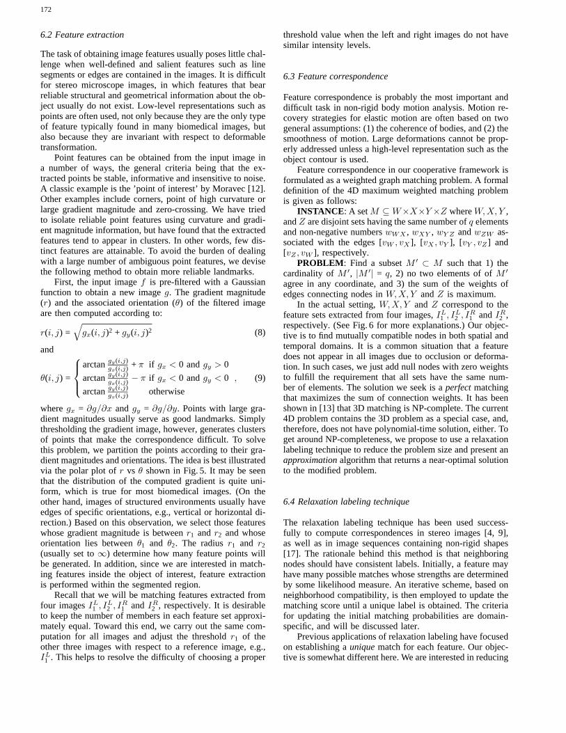
6.2 Feature extraction

The task of obtaining image features usually poses little chal-lenge when well-defined and salient features such as linesegments or edges are contained in the images. It is difficultfor stereo microscope images, in which features that bearreliable structural and geometrical information about the ob-ject usually do not exist. Low-level representations such aspoints are often used, not only because they are the only typeof feature typically found in many biomedical images, butalso because they are invariant with respect to deformabletransformation.

Point features can be obtained from the input image ina number of ways, the general criteria being that the ex-tracted points be stable, informative and insensitive to noise.A classic example is the ’point of interest’ by Moravec [12].Other examples include corners, point of high curvature orlarge gradient magnitude and zero-crossing. We have triedto isolate reliable point features using curvature and gradi-ent magnitude information, but have found that the extractedfeatures tend to appear in clusters. In other words, few dis-tinct features are attainable. To avoid the burden of dealingwith a large number of ambiguous point features, we devisethe following method to obtain more reliable landmarks.

First, the input imagef is pre-filtered with a Gaussianfunction to obtain a new imageg. The gradient magnitude(r) and the associated orientation (θ) of the filtered imageare then computed according to:

r(i, j) =√gx(i, j)2 + gy(i, j)2 (8)

and

θ(i, j) =

arctangy(i,j)

gx(i,j) + π if gx < 0 andgy > 0

arctangy(i,j)gx(i,j) − π if gx < 0 andgy < 0

arctangy(i,j)gx(i,j) otherwise

, (9)

wheregx = ∂g/∂x andgy = ∂g/∂y. Points with large gra-dient magnitudes usually serve as good landmarks. Simplythresholding the gradient image, however, generates clustersof points that make the correspondence difficult. To solvethis problem, we partition the points according to their gra-dient magnitudes and orientations. The idea is best illustratedvia the polar plot ofr vs θ shown in Fig. 5. It may be seenthat the distribution of the computed gradient is quite uni-form, which is true for most biomedical images. (On theother hand, images of structured environments usually haveedges of specific orientations, e.g., vertical or horizontal di-rection.) Based on this observation, we select those featureswhose gradient magnitude is betweenr1 andr2 and whoseorientation lies betweenθ1 and θ2. The radiusr1 and r2(usually set to∞) determine how many feature points willbe generated. In addition, since we are interested in match-ing features inside the object of interest, feature extractionis performed within the segmented region.

Recall that we will be matching features extracted fromfour imagesIL1 , I

L2 , I

R1 andIR2 , respectively. It is desirable

to keep the number of members in each feature set approxi-mately equal. Toward this end, we carry out the same com-putation for all images and adjust the thresholdr1 of theother three images with respect to a reference image, e.g.,IL1 . This helps to resolve the difficulty of choosing a proper

threshold value when the left and right images do not havesimilar intensity levels.

6.3 Feature correspondence

Feature correspondence is probably the most important anddifficult task in non-rigid body motion analysis. Motion re-covery strategies for elastic motion are often based on twogeneral assumptions: (1) the coherence of bodies, and (2) thesmoothness of motion. Large deformations cannot be prop-erly addressed unless a high-level representation such as theobject contour is used.

Feature correspondence in our cooperative framework isformulated as a weighted graph matching problem. A formaldefinition of the 4D maximum weighted matching problemis given as follows:

INSTANCE : A setM ⊆W×X×Y ×Z whereW,X, Y ,andZ are disjoint sets having the same number ofq elementsand non-negative numberswWX , wXY , wY Z andwZW as-sociated with the edges [vW , vX ], [vX , vY ], [vY , vZ ] and[vZ , vW ], respectively.

PROBLEM : Find a subsetM ′ ⊂ M such that 1) thecardinality ofM ′, |M ′| = q, 2) no two elements of ofM ′agree in any coordinate, and 3) the sum of the weights ofedges connecting nodes inW,X, Y andZ is maximum.

In the actual setting,W,X, Y andZ correspond to thefeature sets extracted from four images,IL1 , I

L2 , I

R1 andIR2 ,

respectively. (See Fig. 6 for more explanations.) Our objec-tive is to find mutually compatible nodes in both spatial andtemporal domains. It is a common situation that a featuredoes not appear in all images due to occlusion or deforma-tion. In such cases, we just add null nodes with zero weightsto fulfill the requirement that all sets have the same num-ber of elements. The solution we seek is aperfectmatchingthat maximizes the sum of connection weights. It has beenshown in [13] that 3D matching is NP-complete. The current4D problem contains the 3D problem as a special case, and,therefore, does not have polynomial-time solution, either. Toget around NP-completeness, we propose to use a relaxationlabeling technique to reduce the problem size and present anapproximationalgorithm that returns a near-optimal solutionto the modified problem.

6.4 Relaxation labeling technique

The relaxation labeling technique has been used success-fully to compute correspondences in stereo images [4, 9],as well as in image sequences containing non-rigid shapes[17]. The rationale behind this method is that neighboringnodes should have consistent labels. Initially, a feature mayhave many possible matches whose strengths are determinedby some likelihood measure. An iterative scheme, based onneighborhood compatibility, is then employed to update thematching score until a unique label is obtained. The criteriafor updating the initial matching probabilities are domain-specific, and will be discussed later.

Previous applications of relaxation labeling have focusedon establishing auniquematch for each feature. Our objec-tive is somewhat different here. We are interested in reducing

173

8

6

7

9

Fig. 6. The cooperative spatial and temporal matching processis cast into a 4D maximum weighted matching problem.W ,X, Y andZ correspond to the feature sets extracted from theimages. The connection weights measure the compatibilitybetween these features

Fig. 7. Smoothness of motion constraint: the directions of theflow vectors should be similar in a neighborhood

Fig. 8.Four-dimensional matching has to be done onlyonceinanalyzing a sequence of stereo images. Subsequent matchingsare reduced to 3D once one of the four links is established

Fig. 9. Registered and segmented images

the number of possible matches, or equivalently, the num-ber of edges with non-zero weights in the graphM . Conse-quently, we stop short of convergence and leave the calcu-lated matching probabilities intact. We also avoid declaringany matchedpair in this intermediate step.

6.4.1 Spatial domain relaxation labeling

The following list summarizes some definitions and symbolsused throughout the discussion.

– B(i): neighboring nodes of nodei.– Ni: number of neighboring nodes for nodei.– P k(i, j): matching probability between nodei and j at

the k-th stage, 0≤ P k(i, j) ≤ 1.

– DP (i, j): disparity between nodei andj.

To begin with, we define a matching score betweenfeature i (in image 1) and featurej (in image 2, ob-tained around the epipolar line of featurei) according to:S(i, j) = 0.5(C(i, j) + 1) whereC is the normalized cross-correlation given in Eq. 1. The initial matching probabilitybetween featuresi andj can then be expressed as:

P 0(i, j) =S(i, j)∑Nj

j=1S(i, j), (10)

whereNj is the number of neighbors for nodej that are’matchable’ with nodei.

For stereo matching (i.e., spatial domain processing), theinitial matching probability is updated according to two cri-

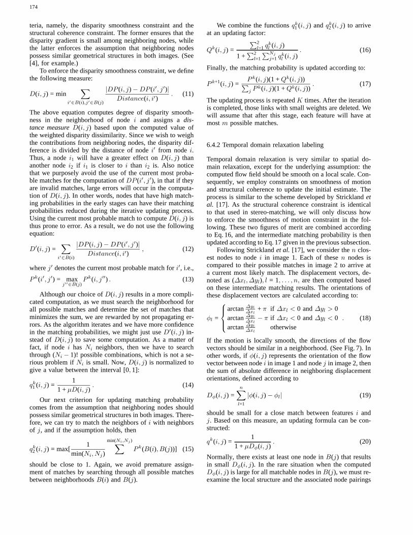
174

teria, namely, the disparity smoothness constraint and thestructural coherence constraint. The former ensures that thedisparity gradient is small among neighboring nodes, whilethe latter enforces the assumption that neighboring nodespossess similar geometrical structures in both images. (See[4], for example.)

To enforce the disparity smoothness constraint, we definethe following measure:

D(i, j) = min∑

i′∈B(i),j′∈B(j)

|DP (i, j)−DP (i′, j′)|Distance(i, i′)

. (11)

The above equation computes degree of disparity smooth-ness in the neighborhood of nodei and assigns adis-tance measureD(i, j) based upon the computed value ofthe weighted disparity dissimilarity. Since we wish to weighthe contributions from neighboring nodes, the disparity dif-ference is divided by the distance of nodei′ from nodei.Thus, a nodei1 will have a greater effect onD(i, j) thananother nodei2 if i1 is closer toi than i2 is. Also noticethat we purposely avoid the use of the current most proba-ble matches for the computation ofDP (i′, j′), in that if theyare invalid matches, large errors will occur in the computa-tion of D(i, j). In other words, nodes that have high match-ing probabilities in the early stages can have their matchingprobabilities reduced during the iterative updating process.Using the current most probable match to computeD(i, j) isthus prone to error. As a result, we do not use the followingequation:

D′(i, j) =∑

i′∈B(i)

|DP (i, j)−DP (i′, j′)|Distance(i, i′)

, (12)

wherej′ denotes the current most probable match fori′, i.e.,

P k(i′, j′) = maxj′′∈B(j)

P k(i, j′′) . (13)

Although our choice ofD(i, j) results in a more compli-cated computation, as we must search the neighborhood forall possible matches and determine the set of matches thatminimizes the sum, we are rewarded by not propagating er-rors. As the algorithm iterates and we have more confidencein the matching probabilities, we might just useD′(i, j) in-stead ofD(i, j) to save some computation. As a matter offact, if node i hasNi neighbors, then we have to searchthrough (Ni − 1)! possible combinations, which is not a se-rious problem ifNi is small. Now,D(i, j) is normalized togive a value between the interval [0, 1]:

qk1 (i, j) =1

1 +µD(i, j). (14)

Our next criterion for updating matching probabilitycomes from the assumption that neighboring nodes shouldpossess similar geometrical structures in both images. There-fore, we can try to match the neighbors ofi with neighborsof j, and if the assumption holds, then

qk2 (i, j) = max[1

min(Ni, Nj)

min(Ni,Nj )∑P k(B(i), B(j))] (15)

should be close to 1. Again, we avoid premature assign-ment of matches by searching through all possible matchesbetween neighborhoodsB(i) andB(j).

We combine the functionsqk1 (i, j) andqk2 (i, j) to arriveat an updating factor:

Qk(i, j) =

∑2l=1 q

kl (i, j)

1 +∑2

l=1

∑Nj

j=1 qkl (i, j)

. (16)

Finally, the matching probability is updated according to:

P k+1(i, j) =P k(i, j)(1 +Qk(i, j))∑j P

k(i, j)(1 +Qk(i, j)). (17)

The updating process is repeatedK times. After the iterationis completed, those links with small weights are deleted. Wewill assume that after this stage, each feature will have atmostm possible matches.

6.4.2 Temporal domain relaxation labeling

Temporal domain relaxation is very similar to spatial do-main relaxation, except for the underlying assumption: thecomputed flow field should be smooth on a local scale. Con-sequently, we employ constraints on smoothness of motionand structural coherence to update the initial estimate. Theprocess is similar to the scheme developed by Stricklandetal. [17]. As the structural coherence constraint is identicalto that used in stereo-matching, we will only discuss howto enforce the smoothness of motion constraint in the fol-lowing. These two figures of merit are combined accordingto Eq. 16, and the intermediate matching probability is thenupdated according to Eq. 17 given in the previous subsection.

Following Stricklandet al. [17], we consider then clos-est nodes to nodei in image 1. Each of thesen nodes iscompared to their possible matches in image 2 to arrive ata current most likely match. The displacement vectors, de-noted as (∆xl, ∆yl), l = 1, . . . , n, are then computed basedon these intermediate matching results. The orientations ofthese displacement vectors are calculated according to:

φl =

arctan∆yl∆xl

+ π if ∆xl < 0 and∆yl > 0arctan∆yl∆xl

− π if ∆xl < 0 and∆yl < 0arctan∆yl∆xl

otherwise. (18)

If the motion is locally smooth, the directions of the flowvectors should be similar in a neighborhood. (See Fig. 7). Inother words, ifφ(i, j) represents the orientation of the flowvector between nodei in image 1 and nodej in image 2, thenthe sum of absolute difference in neighboring displacementorientations, defined according to

Dφ(i, j) =n∑l=1

|φ(i, j)− φl| (19)

should be small for a close match between featuresi andj. Based on this measure, an updating formula can be con-structed:

qk(i, j) =1

1 +µDφ(i, j). (20)

Normally, there exists at least one node inB(j) that resultsin small Dφ(i, j). In the rare situation when the computedDφ(i, j) is large for all matchable nodes inB(j), we must re-examine the local structure and the associated node pairings

175

carefully. Large direction differences indicate that the localmotion pattern is not uniform, i.e., the smoothness assump-tion is violated. Such a violation is generally caused by theerror in the intermediate matching stage, in which a seem-ingly promising match is actually a bad one. When this is thecase, we have to resort to the exhaustive search method sim-ilar to that used in spatial domain relaxation to better resolvethe possible ambiguity. In other words, the measurement ofthe displacement orientation mismatchDφ(i, j) should takean alternate form:

Dφ(i, j) = min∑

i′∈B(i),j′∈B(j)

|φ(i, j)− φ(i′, j′)| . (21)

6.5 Approximation algorithm

We have reduced the problem size by applying relaxationlabeling techniques in both the spatial and temporal do-mains. Even so, solving this reduced problem still requiresan exponential search. We have developed an approximationalgorithm for this modified problem based on the greedy-type search method. The search starts with the edge hav-ing the largest weight so far. A consistency check betweenthe spatial and temporal matching is achieved by maximiz-ing the weights associated with edge connectivity using anexhaustive search, which hasO(m3) complexity. The fournodes connected by these edges are grouped and marked asa matchedquadruple. Then, these nodes and their associatededges are deleted from the graph. The process is repeateduntil the graph becomes empty or the connection weightsare lower than some pre-defined threshold. It can be easilyseen that the worst case computational complexity for theoverall processing isO(qm3). The local search algorithm isoutlined as follows:

/* Local Search Algorithm */Given a graph M with four disjoint sets: W,X, Y, Z,edges [vW , vX ], [vX , vY ], [vY , vZ ] and [vZ , vW ],and weights associated with the edges,BEGINWhile M /= null and weights ≥ wmin do beginTake the edge with largest weight, vi,jFollowing the clockwise direction, connect thenodes such that the weights of vj,k, vk,l, vl,m are thelargest,( j, k, l and m are nodes from each of the four sets)If i = m, record i, j, k, l as a matched quarduple,Else find the best match by exhaustive search.EndifDelete nodes i, j, k, l and adjacent edges from MEnd whileEND

It is possible to further reduce the computational com-plexity by observing that the 4D matching needs to be per-formed onlyoncein analyzing a series of stereo images. Af-ter that, the stereo correspondence betweenIL2 and IR2 hasbeen established, and the subsequent cooperative matchingprocesses are simplified to 3D, whose complexity isO(qm2)(See Fig. 8).

Table 1. Area change of a frog’s ventricle in a series of five frames

Frame Area Normalized area1 44162 1.02 43538 0.9853 42647 0.9654 40553 0.9185 40185 0.909

Table 2. Volume change of a frog’s ventricle in a series of five frames

Frame Volume Normalized volume1 18354 1.02 16885 0.923 15860 0.864 13514 0.7365 12780 0.696

7 Experimental results

The algorithms described above were applied to a sequenceof SLM images of a frog ventricle, as shown in Fig. 2. Thevertical disparity between the stereo images was found tobe 55 pixels. Using the segmentation procedure discussedin Sect. 5, we obtained approximate ROIs for these images.(See Fig. 9.) We inferred from the images that the ventricleis in its contracting phase. In the cooperative matching pro-cess, we elect to usepoint features, not only because theyare usually the only type of features found in many biomed-ical images, but also because they are invariant with respectto deformable transformation. Figure 10 depicts the pointfeatures extracted within the segmented region. The initialmatching probability was assigned according to Eq. 10 andthe updating process was repeated five times. The resultswere then input to the approximation algorithm to estab-lish correspondence. Three-dimensional structure and mo-tion parameters were easily obtained once the correspon-dences were found, as shown in Figs. 11 and 12. We haveused the bilinear interpolation technique to reconstruct the3D data for simplicity.

The change in the object area can be quantified by mea-suring the area of the extracted ROI. On the other hand,visible object volume can be computed from the interpo-lated 3D structure in the following manner. Treating onepixel f (i, j) in the image as a block with base sized × dand heighthi,j , the volume of this rectangular element isexpressed according to:

∆v = d2hi,j . (22)

The total visible volumeV is obtained by summing all∆v

over the object area. Using these strategies, the amount ofarea and volume change of the frog’s ventricle is calculatedand listed in Table 1 and 2. Each frame is about 0.1 s apart,and a series of five frames comprise approximately half theperiod of the heartbeat cycle.

It is desirable to verify the accuracy of the shape param-eters obtained using the proposed method. Due to the natureof the application considered in this research, however, itis extremely difficult, if not impossible, to directly verifythe accuracy of the reconstructed information. (Consider thesize of the object as well as the type of motion exhibitedby live biological specimen.) We have, therefore, elected totest the usefulness of the proposed algorithms in two dif-

176

1310

12

11

Fig. 10. Extracted point features inside the segmented region

Fig. 11. Extracted image features and their associated dispar-ity values in two consecutive frames

Fig. 12. Left: Original image sequence.Right: Reconstructed3D structure

Fig. 13. Features 1–6are manually registered to obtain theground truth disparity value

Table 3. Area change of a frog’s ventricle in a sequence of five cycles

Cycle Frame 1 area Frame 2 area Frame 3 area Frame 4 area Frame 5 area1 44162(100%) 43538(98.5%) 42467(96.5%) 40533(91.8%) 40185(90.9%)2 44057(100%) 43484(98.7%) 42426(96.3%) 40528(92.0%) 40136(91.1%)3 43989(100%) 43285(98.4%) 42317(96.3%) 40514(92.1%) 40030(91.0%)4 44205(100%) 43496(98.4%) 42486(96.1%) 40620(91.9%) 40135(90.8%)5 44136(100%) 43518(98.6%) 42630(96.6%) 40604(92.0%) 40156(91.0%)

177

Table 4. Volume change of a frog’s ventricle in a sequence of five cycles

Cycle Frame 1 vol. Frame 2 vol. Frame 3 vol. Frame 4 vol. Frame 5 vol.1 18354(100%) 16885(92.0%) 15860(86.0%) 13514(73.6%) 12780(69.6%)2 18286(100%) 16914(92.5%) 15689(85.8%) 13568(74.2%) 12782(69.9%)3 18205(100%) 16767(92.1%) 15602(85.7%) 13526(74.3%) 12744(70.0%)4 18410(100%) 16974(92.2%) 15741(85.5%) 13586(73.8%) 12795(69.5%)5 18333(100%) 16921(92.3%) 15766(86.0%) 13579(74.1%) 12804(69.8%)

Table 5. Comparison of the recovered disparity values for features in se-lected regions in a series of five frames.Numbers in parenthesesindicatemanually restored data

Feature Frame 1 Frame 2 Frame 3 Frame 4 Frame 51 103(103) 101(100) 98(98) 94(95) 92(92)2 101(100) 99(99) 97(96) 93(93) 90(89)3 108(108) 107(106) 103(102) 99(99) 97(97)4 104(103) 101(100) 99(98) 93(93) 91(90)5 102(103) 99(99) 96(97) 93(94) 91(91)6 98(99) 96(96) 94(93) 89(89) 87(86)

ferent ways: (1) by testing the consistency of the calculatedglobal shape parameters, and (2) by comparing the resultswith those registered manually in selected regions.

Since the motion exhibited by the ventricle is approxi-mately periodic, we have performed the analysis on the samefrog ventricle undergoing similar deformation in differentheartbeat cycles. The settings of microscope and the light-ing conditions are kept constant during image acquisition.As a result, we expect that the calculated shape parameterswill be approximately equal in different cycles. In Tables 3and 4, we list the change in object area and visible volumefor the same specimen in different cycles. Each frame is0.1 s apart. These results confirm the repeatability of the ex-periment and, to a certain extent, verify the consistency ofthe proposed algorithms.

To verify the correctness of the recovered local defor-mation, direct measurements are performed on the regionswhere maximum height changes are likely to occur. Specifi-cally, we have manually registered six features on each heartsurface, as shown in Fig. 13. The results are then comparedwith the disparity values obtained using the proposed algo-rithms, as tabulated in Table 5. Even though the true disparitycannot be obtained everywhere, the depth information re-stored in the selected regions agrees closely with the groundtruth.

8 Conclusions

In summary, we present a framework for quantifying thedynamic shape characteristics of biological specimens im-aged through a SLM. We demonstrate the effectiveness ofthe cooperative matching process on a series of binocularimages containing non-rigid objects. The reconstructed dy-namic structure of the biological specimen agrees qualita-tively with the observed motion sequence. The accuracy ofthe recovered information is verified using two testing pro-cedures. Currently, we are studying the imaging geometry ofthe stereo microscope and investigating a reliable calibrationprocedure for SLM images. Once such work is completed, afully automated system can be developed to perform quan-titative analysis of the imaged specimen in an accurate and

consistent manner. Of course, one has to keep in mind cer-tain limitations of the SLM in obtaining the 3D informationof the observed specimen. For example, only visible surfacearea and volume can be restored, and these results dependon the viewing angle as well as the distribution of the fea-tures. Consequently, care must be exercised in interpretingthe meaning of the recovered data.

Acknowledgements.This work was supported by the National ScienceFoundation, contract BIR-9106624.

References

1. Aggarwal JK, Cai Q, Liao W, Sabadta B (1994) Articulated and elasticnon-rigid motion: a review. In: Proc of the IEEE Workshop on Motionof Non-rigid and Articulated Objects, pp 2–14

2. Aggarwal JK, Nandhakumar N (1988) On the computation of motionfrom image sequences: a review. Proc IEEE 76:917–935

3. Amini AA, Duncan JS (1991) Pointwise tracking of left-vertricularmotion in 3D. In: Proceedings of Computer Vision and Pattern Recog-nition, pp 294–299

4. Barnard ST, Thompson WB (1980) Disparity Analysis of Images, IEEETrans PAMI 2:333–340

5. Bartels K, Bovik A, Aggarwal SJ, Diller KR (1992) Shape changeanalysis of confocal microscope images using variational techniques.Proc. SPIE Conf. Biomedical Image Processing and Three-DimensionalMicroscopy. SPIE 1660:618–629

6. Chen CW, Huang TS (1991) Surface modeling in heart motion analysisProc. Conf. Curves and Surfaces in Computer Vision and Graphics.SPIE 1610:360–371

7. Cohen LD, Cohen I (1992) Deformable models for 3D medical imagesusing finite elements and balloons. In: Proceedings of InternationalConference on Pattern Recognition. pp 592–598

8. Dhond UR, Aggarwal JK (1989) Structure from stereo – a review.IEEE Trans Syst Man Cybern 19:1489–1510

9. Hummel RA, Zucker SW (1983) On the foundations of relaxationlabeling processes, IEEE Trans PAMI 5:267–287

10. Kass M, Witkin A, Terzopoulos D (1987) Snakes: active contour mod-els. Int J Comput Vision 1:312–331

11. Kim N, Bovik AC, Aggarwal SJ (1990) Shape description of biologicalobjects via stereo light microscopy, IEEE Trans System Man Cybern20:475–489

12. Moravec H (1981) Robot rover visual navigation, U.M.I. ResearchPress, Ann Arbor, MI

13. Papadimitriou CH, Steiglitz K (1982) Combinatorial optimization: al-gorithms and complexity. Prentice-Hall, Englewood Cliffs, New Jersey

14. Reimer L (1985) Scanning electron microscopy: physics of image for-mation and microanalysis. Springer Berlin Heidelberg New York

15. Shapiro LS, Wang H, Brady JM (1992) A matching and tracking strat-egy for independently moving objects. In: Proc. British Machine VisionConference, pp 306–315

16. Staib LH, Duncan JS (1992) Deformable Fourier models for surface-finding in 3D images. Proc. Conf. Visualization in Biomedical Com-puting, SPIE 1808:90–104

17. Strickland RN, Mao Z (1992) Computing correspondences in a se-quence of non-rigid shapes. Pattern Recognition 25:901–912

18. Waxman AM, Duncan JH (1986) Binocular Image Flows: steps towardstereo-motion fusion. IEEE Trans. on PAMI 8:715–729

178

J. K. Aggarwal is Cullen Professor of Electrical and Computer Engi-neering and Director of the Computer and Vision Research Center at TheUniversity of Texas at Austin, where he has served on the faculty since1964. His research interests include computer vision, parallel processingof images, and pattern recognition. An IEEE Fellow since 1976, he wasrecently named as the recipient of the 1996 Technical Achievement Awardof the IEEE Computer Society. He is author or editor of 7 books and 31book chapters; author of over 160 journal papers, as well as numerousproceedings papers and technical reports.

Wen-Hung Liao received the B.S. degree from the Department of Electri-cal Engineering of National Taiwan University, Taipei, in June 1987 and theM.S.E.E. degree from the Department of Electrical and Computer Engineer-ing of the University of Texas at Austin in August 1991. He is currently aPh.D. candidate in the Department of Electrical and Computer Engineeringof the University of Texas at Austin. His research interests include computervision, biomedical image processing, quantitative microscopy and non-rigidmotion anlysis.

Shanti J. Aggarwal received the M.S. and Ph.D. degrees in microbiol-ogy from the University of Michigan in 1958 and 1962, respectively. Shejoined the University of Texas at Austin in 1965 and taught immunologyand biology while actively doing research in immunology. In 1982, shejoined Department of Mechanical Engineering and Biomedical EngineeringProgram. Dr. Aggarwal has published numerous papers in immunology,cryobiology, and microcirculatory physiology. Her current research inter-ests include the application of computers and computer vision in biology.