The Rebound Effect for Passenger Vehicles - rff.org · 1616 P St. NW Washington, DC 20036 202-328-5000 July 2013 RFF DP 13-19 The Rebound Effect for Passenger Vehicles DISCUSSION

1616 P St. NW Washington, DC 20036 202-328-5000 www.rff.org

July 2013 RFF DP 13-19

The Rebound Effect for Passenger Vehicles

Joshua L i nn

DIS

CU

SS

ION

PA

PE

R

© 2013 Resources for the Future. All rights reserved. No portion of this paper may be reproduced without

permission of the authors.

Discussion papers are research materials circulated by their authors for purposes of information and discussion.

They have not necessarily undergone formal peer review.


Joshua Linn

Abstract

Increasingly stringent fuel economy standards will reduce per-mile driving costs and may raise

vehicle miles traveled, which is referred to as the rebound effect. All previous estimates impose at least

one of three behavioral assumptions: (a) fuel economy is uncorrelated with other vehicle attributes; (b)

fuel economy is uncorrelated with attributes of other vehicles owned by the household; and (c) the effect

of gasoline prices on vehicle miles traveled is inversely proportional to the effect of fuel economy.

Relaxing these assumptions yields a large and robust rebound effect; a one percent fuel economy increase

raises driving 0.2 to 0.4 percent.

Key Words: fuel economy standards, passenger vehicles, vehicle miles traveled, household

driving demand

JEL Classification Numbers: Q52, R22, R41

Contents

1. Introduction ......................................................................................................................... 1

2. Simple Model of Household Driving Decisions ................................................................ 5

2.1 Miles Traveled for a Single-Vehicle Household (Assumption (a)) .............................. 5

2.2 Multivehicle Households (Assumption (b)).................................................................. 7

2.3 Persistence and the Long-Run Effects of Gasoline Prices and Fuel

Economy (Assumption (c)) ........................................................................................... 8

3. Estimation Strategy ............................................................................................................ 9

4. Data and Summary Statistics ........................................................................................... 13

4.1 Data ............................................................................................................................. 13

4.2 Summary Statistics and the Exogeneity of Gasoline Prices ....................................... 14

5. Estimation Results ............................................................................................................ 15

5.1 Main Results ............................................................................................................... 15

5.2 Robustness of the Main Specification ......................................................................... 17

5.3 Implications of Imposing Assumptions (a)–(c) .......................................................... 18

6. Rebound Effect for Hypothetical Fuel Economy Increases .......................................... 19

7. Conclusions ........................................................................................................................ 20

References .............................................................................................................................. 22

Figures and Tables ................................................................................................................ 23

Resources for the Future Linn

1


Joshua Linn

1. Introduction

Motivated by a desire to reduce gasoline consumption and the associated external energy

security and climate costs, the US fuel economy standards for new passenger vehicles will

dramatically increase average new vehicle fuel economy. The current standards, which the US

Environmental Protection Agency (US EPA) and the US Department of Transportation set

jointly, raise average fuel economy to roughly 35 miles per gallon (mpg) by 2016. This level

represents a roughly 40 percent increase compared to the standards in the mid-2000s. The

recently finalized 2025 standards could raise fuel economy by an additional 50 percent, to

roughly 54 mpg.

A large literature has compared the cost of reducing gasoline consumption by using fuel

economy standards with the cost of using the gasoline tax (e.g., Jacobsen 2013). A central

conclusion has been that the gasoline tax is much less costly to vehicle producers and consumers

per gallon of gasoline saved. An important difference between fuel economy standards and a

gasoline tax is the rebound effect, whereby fuel economy standards decrease the per-mile cost of

driving, increasing miles traveled and offsetting some of the fuel savings.1 Considering a

hypothetical standard that raises average fuel economy by a particular amount, the larger the

rebound effect, the lower the fuel savings will be, and the higher the cost of the standards per

gallon of gasoline saved. Thus, welfare analysis depends crucially on the magnitude of the

rebound effect.

Past studies have reported a wide range of estimates, which imply that a 1 percent fuel

economy increase raises driving 0.1 to 0.8 percent. Most estimates fall in the range of 0.1 to 0.3

(US EPA 2011), and many recent estimates have fallen toward the lower end. Based on the

results of several recent studies, the federal government uses an elasticity of 0.1 for estimating

Fellow, Resources for the Future; I thank Kevin Bolon and Ken Gillingham for comments on an earlier draft.

Shefali Khanna provided excellent research assistance. Email: [email protected].

1 This is often referred to as the “direct” rebound effect, which is distinct from the “indirect” rebound effect that

arises from the income increase for households that spend less on energy services after adopting technology that

raises energy efficiency (Gillingham et al. 2013).


2

the fuel savings of the upcoming fuel economy standards. But the cost of fuel economy standards

per gallon of gasoline saved could vary substantially depending on the actual rebound effect.

Whether using aggregate or micro data on fuel economy and vehicle miles traveled

(VMT), there are several major challenges to estimating the rebound effect from variation in the

two variables. First, because households choose the fuel economy of their vehicles, fuel economy

may be correlated with other attributes of the vehicle or household that are hard to control for

and which may bias econometric estimates of the rebound effect. Second, and following from the

first, the short-run rebound effect probably differs from the long-run rebound effect because

households adjust their behavior gradually—such as by carpooling, moving, or changing jobs.

The long-run rebound effect is more relevant to policy analysis than the short-run rebound effect,

but estimating long-run rebound introduces the typical challenges of estimating long run

responses while controlling for other factors that affect VMT such as income.

In this paper, I argue that, to avoid these challenges, every study in the rebound literature

has made at least one of three assumptions about consumer behavior. The paper’s objective is to

simultaneously relax these assumptions and obtain an unbiased estimate of the long-run rebound

effect. The first assumption is that fuel economy is uncorrelated with other vehicle attributes that

affect a consumer’s utility from driving. Studies based on time series variation in aggregate

average fuel economy (e.g., Small and van Dender 2007), or studies using micro data that do not

include vehicle fixed effects or extensive controls for vehicle characteristics, implicitly assume

that fuel economy is uncorrelated with other vehicle attributes, such as engine power or

reliability. However, Klier and Linn (2012) argue that because of the vehicle design process, fuel

economy is likely to be correlated with attributes that can be measured (such as power) and

attributes that are harder to measure (such as reliability). If fuel economy is negatively correlated

with such attributes, failing to control for them would bias empirical estimates of the rebound

effect toward zero.

The second assumption maintained in most of the rebound literature is that, for

multivehicle households, the VMT for one vehicle is independent of the VMT for another

vehicle. Or, in other words, the fuel economy of one vehicle is uncorrelated with the fuel

economy and other attributes of the other vehicle(s). This seems unlikely, however, if the use of

a vehicle for a particular purpose depends on its fuel economy. For example, a household may

use a small car for a long commute and a large sport utility vehicle (SUV) for local shopping

trips. With the exception of Feng et al. (2005) and Spiller (2012), econometric analysis of the

demand for VMT and gasoline treats each of a household’s vehicles as an independent

observation.


3

The third assumption is that VMT responds similarly to gasoline prices and fuel

economy. Many recent studies have analyzed the effect of gasoline prices on VMT (e.g.,

Gillingham 2013). Such an analysis is appropriate for quantifying the effects of gasoline prices

on gasoline consumption. However, most studies that have estimated a rebound effect for

purposes of evaluating fuel economy standards have estimated the elasticity of VMT to the fuel

price or to fuel costs. The implicit assumption is that fuel economy and fuel prices affect VMT

by equal and opposite amounts. This assumption may not hold in practice. For example, if

consumers expect gasoline price shocks to be temporary and changing VMT (e.g., by arranging

for carpooling) has fixed costs, VMT would respond less to a gasoline price decrease than to a

proportional fuel economy increase. Anderson et al. (2011) conclude that, on average, consumers

believe gasoline price shocks to be permanent. The authors also report considerable

heterogeneity in consumer beliefs, which suggests that, for many consumers, VMT may respond

differently to gasoline prices than to fuel economy. Of the few studies that estimate the effect of

fuel economy on VMT, Gillingham (2012) finds that fuel economy affects VMT less than fuel

prices, Frondel et al. (2012) and Small and van Dender (2007) report no difference between the

two effects, and Greene (2012) reports a difference in some specifications. However, the latter

two studies use aggregate data and time series variation in fuel economy, making it difficult to

identify the effect of fuel economy on VMT. Fuel economy changes gradually over time and

such changes may be correlated with other determinants of VMT that are difficult to measure,

such as congestion.

This paper shows that simultaneously relaxing these assumptions significantly raises the

estimated rebound effect. The first part of the paper demonstrates the empirical implications of

maintaining the three assumptions held in the literature: (a) fuel economy is uncorrelated with

other vehicle characteristics; (b) for multivehicle households, vehicles can be treated as unique

observations; and (c) VMT responds similarly to fuel prices and to fuel economy. I show that if

fuel economy is negatively correlated with unobserved vehicle characteristics, estimating the

rebound effect but failing to account for unobserved vehicle characteristics biases the estimated

rebound effect toward zero. Failing to account for the interdependence of VMT among vehicles

in multivehicle households biases the estimate, but the direction of the bias is theoretically

ambiguous. Finally, assuming that consumers respond similarly to fuel prices and fuel economy

creates downward bias of the fuel economy rebound effect if the rebound effect is estimated

using gasoline price variation and consumers have different beliefs about the persistence of

gasoline prices and vehicle fuel economy.


4

The second part of the paper uses recent survey data to implement a simple linear

regression that relaxes the three assumptions. Using household data from the 2009 National

Household Travel Survey (NHTS), I estimate the effects on VMT of gasoline prices and fuel

economy. The dependent variable is VMT by vehicle, and the independent variables include the

current gasoline price, the vehicle’s fuel economy, and household and vehicle characteristics. I

relax the first assumption by including vehicle model fixed effects and by instrumenting for the

vehicle’s fuel economy. The instrument is the gasoline price at the time the vehicle was

purchased. This approach, which is similar to that of Allcott and Wozny (2012), rests on the

strong correlation between fuel prices and new vehicle fuel economy documented by Klier and

Linn (2010) and Busse et al. (2013), among others. Based on the simple model in Section 2 and

similar to Feng et al. (2005), I account for the effects of the household’s other vehicles by

controlling for their average fuel economy. Finally, to relax the third assumption, I estimate

separate coefficients on gasoline prices and vehicle fuel economy.

I find that VMT responds much more strongly to vehicle fuel economy than to gasoline

prices. Across specifications, the elasticity of VMT to gasoline prices is –0.06 to –0.2, but the

estimates are seldom statistically significant across regression models. I refer to the fuel

economy rebound effect as the effect on VMT of a 1 percent increase in the fuel economy of all

vehicles belonging to a household. The rebound effect ranges from 0.2 to 0.4. The fuel economy

estimates are statistically significant in nearly all specifications.

I next show the importance of relaxing the three assumptions that the rebound literature

has imposed. The rebound effect is much larger after addressing the potential correlation

between fuel economy and other vehicle characteristics. Controlling for other vehicles’ fuel

economy reduces the estimated rebound effect for multivehicle households. The estimated

rebound effect is much larger relaxing the assumption that the effect of gasoline prices on VMT

is inversely proportional to the effect of fuel economy on VMT. Thus, all three assumptions

prove to be empirically important.

Finally, I use the results to estimate the effect on VMT and gasoline consumption of

future fuel economy increases caused by higher standards. I consider two scenarios to

characterize the effects of the 2016 fuel economy standards on VMT. In the first scenario, fuel

economy of all vehicles increases 44 percent, which is the average fuel economy increase

predicted by US EPA (2011) for the 2011–2016 standards for the vehicles in my sample. Such an

increase would reduce gasoline consumption by about 31 percent in the absence of a rebound

effect. The baseline estimates suggest that VMT increases 14 percent and erodes about one-third

of the reduction in gasoline consumption. The second scenario uses the fuel economy changes


5

for each vehicle model predicted by the National Highway Traffic Safety Administration in its

analysis of the 2016 fuel economy standards (US EPA 2011). The results for this scenario

similarly suggest that the rebound effect reduces the gasoline consumption savings by about one-

third.

2. Simple Model of Household Driving Decisions

Most empirical studies of consumer demand for VMT, and particularly those using

household-level data, derive an estimating equation from an assumed utility function. I specify a

utility function and demonstrate the potential bias from imposing each of the three assumptions

discussed in the Introduction.

2.1 Miles Traveled for a Single-Vehicle Household (Assumption (a))

Consider a household endowed with a single vehicle and income, I . The vehicle provides

services to the household so that the household’s utility,U , depends on theVMT of the vehicle

and on the consumption of good y , which represents all other goods in the economy.

The vehicle’s fuel economy is m and the variable represents the vehicle’s “quality.”

The variable is known to the household but cannot be observed by the econometrician.

The household’s utility is:

( / )U VMT y , (1)

where 0 . Utility is increasing in VMT and vehicle quality. The marginal utility of VMT

decreases with VMT to reflect the fact that some driving purposes are more valuable than others.

A vehicle with higher quality confers greater utility because driving the vehicle is more

enjoyable. The marginal utility of vehicle quality decreases with quality.

The household’s budget constraint is:

y+p*VMT

m= I ,

where pis the price of gasoline, and the price of y is normalized to 1. The vehicle’s per-mile fuel

cost is p /m .

The household chooses VMT and y to maximize utility, subject to the budget constraint.

Rearranging the VMT first-order condition yields a log-linear equation betweenVMT , per-mile

fuel costs, and vehicle quality:


6

1 1ln( ) ln( ) ln( ) ln( )

1 1 1

pVMT

m

(2)

where the first term is a constant. Because 0 , VMT decreases with per-mile fuel costs and

increases with vehicle quality.

It is possible to use equation (2) as the basis for estimating the rebound effect. For

example, equation (2) can be estimated by ordinary least squares (OLS) using household-level

survey data on VMT and per-mile fuel costs and by assuming that the vehicle quality term is

uncorrelated with per-mile fuel costs. The fuel cost coefficient can be interpreted as the estimate

of the rebound effect, such that a 1 percent reduction in per-mile fuel costs increases VMT by

11

.

However, such an estimate of the rebound effect is unbiased only under assumption (a),

that vehicle quality is uncorrelated with per-mile fuel costs. If the assumption does not hold and

if vehicle quality is negatively correlated with fuel economy, the estimated rebound effect is

biased toward zero. Whether (unobserved) quality is correlated with fuel economy is, of course,

impossible to test using existing data. However, because consumer demand and production costs

affect vehicle manufactures’ choices of fuel economy and quality (Klier and Linn 2012), the

correlation between fuel economy and quality is probably different from zero. It is not obvious

whether the correlation is positive or negative; therefore, the direction of the resulting bias of

estimating equation (2) by OLS is ambiguous.

Despite the simplicity of the modeling environment and the utility function, this

conclusion applies to much more sophisticated models and utility functions. For example, I

assume that utility is the sum of two terms: the consumption of all other goods and a constant

elasticity term involving VMT and vehicle quality. This functional form results in the log-

linearity of equation (2). Relaxing the assumption that the utility from driving is separable from

the utility from consuming good y would result in a more complicated expression than equation

(2), and most likely one that could not be estimated by OLS. However, the same conclusion

would apply, namely that failing to account for the correlation between unobserved vehicle

quality and fuel costs would result in a biased estimate of the rebound effect.

Another simplification in the preceding analysis is that the household is endowed with

one vehicle. In contrast, many papers analyzing demand for VMT or for gasoline also model the

household’s vehicle choice (e.g., West 2004; Bento et al. 2009). The rationale for jointly

modeling vehicle choice and VMT is that unobserved household characteristics may be


7

correlated with both the vehicle’s fuel economy andVMT . Jointly modeling these decisions

makes it possible to account for the correlation between household characteristics and fuel

economy. However, this approach does not account for the potential correlation between fuel

economy and vehicle characteristics. In short, allowing for the correlation between household

characteristics and fuel costs does not eliminate the bias caused by the correlation between

vehicle characteristics and fuel costs.

2.2 Multivehicle Households (Assumption (b))

The previous discussion imposes assumption (b): for multivehicle households, the fuel

economy of other vehicles does not affect the fuel economy of the particular vehicle. To relax

this assumption, I consider a household that owns two vehicles, 1,2j . The utility function is:

1 1 2 2( / ) ( / )U VMT VMT y ,

where 0 . Because the utility function is multiplicative in the utility from the two

vehicles, driving one vehicle more raises the marginal utility of driving the other vehicle. This

assumption embodies the household’s ability to allocate the vehicles to the most suitable uses—

for example, using the SUV for shopping trips and the car for commuting. The household’s

budget constraint is similarly modified to include the second vehicle.

Rearranging the first-order conditions from the resulting optimization problem yields the

two-vehicle analog of equation (2):

1 0 1 2

1 2

ln( ) ln( ) ln( )p p

VMTm m

(3)

where

0

1ln( ) ln( )

1 1

,

1

1

1

,

21

, and

1 2ln( ) ln( )1 1

.


8

Given the assumptions on the utility function parameters, the fuel costs of vehicle 1 negatively

affect VMT1 and the fuel costs of vehicle 2 positively affectVMT

1. The error term now includes

the quality of both vehicles.

Estimating equation (3) and omitting the other vehicle’s fuel costs and quality may bias

the estimated rebound effect (i.e., 1 ) for two reasons. First, the vehicle’s fuel economy ( 1m )

may be correlated with the other vehicle’s fuel economy ( 2m ). Second, the vehicle’s fuel

economy may be correlated with the quality of the other vehicle ( 2 ).

2.3 Persistence and the Long-Run Effects of Gasoline Prices and Fuel Economy (Assumption (c))

So far I have imposed assumption (c), that consumers respond in equal magnitude to the

gasoline price and to fuel economy. Because of this assumption, a single variable in equation (2),

per-mile fuel costs ( p /m), captures the rebound effect. I show that a simple extension of the

basic model allows for the possibility that the effect of the gasoline price on VMT may differ

from the effect of fuel economy onVMT .

I return to the case where the household owns one vehicle, but now I introduce multiple

time periods, 1,2,3t . The household chooses VMT in each time period, but changing VMT

between time periods has a fixed cost. The fixed costs represent adjustment costs, such as finding

someone with whom to carpool or changing jobs. The fixed costs do not depend on the change in

VMT (relaxing this assumption does not affect the conclusions but complicates the expressions).

Suppose that in period 1, the household expects that the price of gasoline equals p in all

three time periods. In that case, the chosen VMT in each period is the same as in equation (2),

which I refer to as *VMT .

Now, consider an unexpected and permanent increase in gasoline prices between periods

1 and 2, to p ' . The household can either change its VMT at the beginning of period 2 or remain

at *VMT . It is straightforward to show that, because of the (fixed) adjustment costs, the

household chooses to remain at *VMT as long as p ' is sufficiently close to p , with p defined

as the price above which the household changes from VMT to 'VMT . That is, *VMT VMT if

p < p ' < p , and if p ' > p , the household reduces VMT to ' *VMT VMT . This result is

connected to the literature on capital investment and adjustment costs; I refer to the range of

prices between p and p as the inaction zone.

Alternatively, suppose that the price increases unexpectedly to 'p between periods 1 and

2, but the household expects the price increase to be temporary so that between periods 2 and 3


9

the price decreases back to p . As with the permanent price increase, the household changes

VMT only if the price increase is sufficiently large. However, the inaction zone is larger for a

temporary price increase than for a permanent one. Consequently, the effect of a temporary price

increase on VMT is smaller than the effect of a permanent price increase on VMT.

This conclusion implies that if households consider gasoline price changes to be less

persistent than the vehicle’s fuel economy, households will change VMT less in response to a

gasoline price increase than to a proportional fuel economy decrease. Presumably, consumers

consider a vehicle’s fuel economy to be highly persistent over its lifetime. Therefore, the validity

of the standard assumption that consumers respond equally to a gasoline price increase as to a

fuel economy decrease (and vice versa) rests on whether consumers consider gasoline price

shocks to be fully persistent (i.e., that prices follow a random walk). Anderson et al. (2011)

conclude that households believe gasoline price shocks are fully persistent on average, but they

find considerable heterogeneity around the average. Therefore, the household response to

gasoline prices may be different from the response to fuel economy. In that case, using variation

in gasoline prices and VMT would yield a biased estimate of the fuel economy rebound effect.

The bias is toward zero if households believe that gasoline price shocks are less persistent than

fuel economy.

3. Estimation Strategy

As defined in the Introduction, the fuel economy rebound effect is the effect on VMT of a

1 percent increase in the fuel economy of all of a household’s vehicles. In the remainder of the

paper, in unambiguous cases, I use the term rebound effect for shorthand. The objective is to

estimate the rebound effect while relaxing the three assumptions discussed in Section 2.

I begin with a version of equation (2) that specifies the VMT of vehicle i belonging to

household h as a function of its fuel costs and household characteristics:

0 1ln( ) ln( / )hi h hi h hiVMT p m X (4)

where phis the price of gasoline; him is the vehicle’s fuel economy; hX is a vector of

characteristics of household h ; and 0 , 1 and are parameters to be estimated. The parameter

1 is the elasticity of VMT to the vehicle’s per-mile fuel costs.

Section 2 shows that estimating equation (4) would yield biased estimates of the rebound

effect for three reasons. First, per-mile fuel costs are correlated with the error term if the

vehicle’s fuel economy is correlated with other characteristics of the vehicle that are not included


10

in equation (4). Second, per-mile fuel costs are correlated with the error term if the vehicle’s fuel

economy is correlated with the fuel economy or quality of other vehicles owned by the

household. Third, VMT may respond differently to gasoline prices than to fuel economy, in

which case 1 does not correspond to the rebound effect as defined in the Introduction.

Given these considerations, I modify equation (4) in three ways. First, I add vehicle

model fixed effects, j and include interactions of the fixed effects with certain household

characteristics. The vehicle model fixed effects control for vehicle characteristics other than fuel

economy, such as horsepower or overall “quality,” which vary at the model level. Note that fuel

economy may vary across vintages of the same model. For example, the fuel economy of the

2002 Toyota Camry averages about 23 mpg (combined US EPA highway and city ratings),

whereas the 2009 Toyota Camry averages about 24 mpg. Therefore, the vehicle model fixed

effects do not absorb all of the variation of him .

Note that, although the model fixed address possible correlation between household

characteristics and model-level vehicle characteristics, the model fixed effects do not control for

vehicle or household characteristics that vary across vintages of the same model. Therefore,

estimating equation (4) and including vehicle model fixed effects may still yield biased results—

even putting aside assumptions (b) and (c). Consequently, I instrument for the vehicle’s fuel

economy using the gasoline price at the time the household purchased the vehicle, p̂hi

. This

gasoline price is different from ph, which is the gasoline price at the time that VMT

hiis measured.

For example, if VMThi

is measured in April 2009 and the household purchased the vehicle in

April 2002, phis the price of gasoline faced by the household in April 2009 and p̂

hiis the price of

gasoline faced by the household in April 2002.

The validity of the fuel economy instrument rests on three arguments. The first is that the

price of gasoline affects the fuel economy of the purchased vehicle. Klier and Linn (2010)

demonstrate a strong relationship between the fuel economy of new vehicle purchases, and

Allcott and Wozny (2010) use a similar instrumental variables (IV) approach to estimate

consumer demand for fuel economy. Note, however, that Busse et al. (2013) find that, for used

vehicles, gasoline prices affect purchase prices more than sales. This suggests that p̂hi

may be a

weaker instrument for used vehicle purchases. In my sample, the effect of p̂hi

on vehicle fuel

economy is about twice as large for vehicles purchased new than for vehicles purchased used,

which is broadly consistent with Busse et al. (2013). However, for both new and used vehicles

the effects are highly statistically significant, which reduces concerns about weak instruments

bias.


11

The second argument for the price instrument is that the correlation between ph(the

current price) and p̂hi

(the price at the time of purchase) is sufficiently low to identify the

coefficients in the second stage. In fact, the correlation between the two gasoline price variables

is close to zero after controlling for the other variables in equation (4).

The third argument is that the gasoline price at the time of purchase is likely to be

uncorrelated with vehicle and household characteristics not included in the estimating equation.

Because equation (5) includes geographic controls, the first stage is identified by the substantial

temporal gasoline price variation (see, e.g., Klier and Linn 2010); the underlying argument is that

the timing of the vehicle purchase is uncorrelated with omitted household characteristics.

Turning to the second assumption in equation (4), I control for the fuel economy of the

household’s other vehicles. For one- or two-vehicle households, controlling for other vehicle fuel

economy is straightforward: for one-vehicle households the variable equals zero, and for two-

vehicle households the variable equals the other vehicle’s fuel economy. For households owning

three or more vehicles, I use the average fuel economy of the other vehicles. An alternative is to

control for the fuel economy of the other vehicles individually, but in that case the household’s

vehicles must be ordered according to some criterion. Section 5.2 reports a few regressions using

specific ordering criteria.

To address the third assumption in equation (4), I simply allow for a separate coefficient

on the contemporaneous gasoline price and the vehicle’s fuel economy. These modifications

yield the following equation:

0 1 2 3 ,ln( ) ln( ) ln( ) ln( ) ( , )hi h hi h i j h hiVMT p m m f X (5)

where ,ln( )h im is the log of the average fuel economy of the household’s other vehicles; the

variable equals zero for one-vehicle households. The function ( , )j hf Z includes an extensive

set of controls for household and vehicle characteristics. Specifically, the regressions contain

controls for demographics including income, education, age, household size, number of drivers,

and number of vehicles; geography including urban area type, metropolitan statistical area

(MSA) size, urban area size, consolidated MSA (CMSA), population density, and household

density; and survey month. Vehicle characteristics include model fixed effects and vehicle age

group fixed effects as well as interactions between model fixed effects and the number of

vehicles belonging to the household. As discussed in Section 4, many of these variables are

categorical rather than continuous, and the regressions include fixed effects for each category.

Note that these controls and interaction terms are far more extensive than those used in most


12

previous estimates of the rebound effect. The ability to include so many control variables is an

advantage of the simple regression approach employed in this paper.

Equation (5) is estimated by IV. The instruments include the interaction of model fixed

effects with the gasoline price at the time of purchase, p̂hi

. These variables instrument for the

vehicle’s fuel economy, him . As Section 2.2 shows, the fuel economy of the household’s other

vehicles may also be correlated with the error term. To address this possibility, I instrument for

,h im using the interaction of model fixed effects with the average price of gasoline at the time the

household’s other vehicles were purchased.2

Despite relaxing assumptions (a)–(c), some potential concerns remain for equation (5).

First, although I instrument for the fuel economy of all vehicles in equation (5), I assume that the

contemporaneous gasoline price, ph, is exogenous. The next section shows that this variable is

not strongly correlated with any of the other variables in equation (5), supporting the exogeneity

assumption.

Second, the primary motivation for the IV strategy was to account for the possible

correlation between fuel economy and other vehicle characteristics. Fuel economy could also be

correlated with household characteristics, but the fuel economy instruments account for this

possibility, thus mitigating the concern. Further supporting the validity of the fuel economy

instruments, Section 5.2 shows that the results are fairly insensitive to controlling even more

flexibly for vehicle or household characteristics.

Third, equation (5) was derived from a very simple functional form for household utility

in Section 2. I interpret the log-linear specification as an approximation of a more complicated

functional relationship. Section 5.2 reports additional specifications of equation (5) that allow the

elasticity to vary across households or vehicles and for other functional forms of the underlying

utility function.

Before proceeding, I note that an alternative to equation (5) would be to jointly estimate

the vehicle choice and VMT decisions. In principle, the joint estimation, of which the literature

includes many examples (e.g., Bento et al. 2009), has two advantages over a standard reduced-

form VMT equation (which imposes assumptions [a]–[c]). First, the joint estimation makes it

2 Including the interactions of gasoline price and model fixed effects improves the fit of the first stage and reduces

the estimated rebound effect in the second stage.


13

possible to control for unobserved household attributes that affect both vehicle choice andVMT .

For example, households with members who like high-performance cars may purchase cars with

low fuel economy, and they may also like to drive more miles than members of other

households. Second, by deriving the estimating equations from a household utility function, joint

estimation enables an analysis of the welfare effects of policies such as gasoline taxes or fuel

economy standards.

As with joint estimation, equation (5) allows for potential correlation between fuel

economy and unobserved household characteristics. An advantage of equation (5) over joint

estimation is that it is much simpler to relax assumptions (a)–(c) without making modeling

compromises that are typically made in joint estimation. For example, most other studies

aggregate across vehicle models to reduce the choice set for computational reasons. The primary

downside to equation (5) is that welfare analysis of particular policies, such as a gasoline tax

increase, is not possible. Nevertheless, equation (5) is suitable for the paper’s primary objective,

which is to obtain a robust estimate of the rebound effect.

4. Data and Summary Statistics

4.1 Data

The 2009 NHTS is the primary data source. The unit of observation is the household and

vehicle. I include all observations without missing values for household characteristics,

geographic information, and vehicle characteristics; the final data set contains 229,851

observations. The data set includes categorical variables for income, household size, number of

adults, and education level. The geographic information includes categorical variables for urban

area type, MSA size, and urban area size. The geographic information also includes continuous

variables for population density and household density.

The vehicle information includes the estimated VMT of the vehicle for the previous year,

the vehicle’s age, its fuel economy, and its make and model. The survey data include the year

and month in which the vehicle was purchased. To construct the gasoline price instruments, I

merge retail gasoline prices from the Energy Information Administration (EIA) for the

corresponding year, state, and month.

Equation (5) includes the current gasoline price. Whereas the price used to construct the

instrumental variables varies by year, state, and month, the current gasoline price varies by city

and month. The NHTS provides gasoline prices, but regional variation is minimal. For this


14

reason, I impute the retail gasoline prices from the American Chamber of Commerce

Researchers’ Association (ACCRA) and EIA prices. The ACCRA prices vary by city and

quarter, whereas the EIA prices vary by state and month. I impute the household’s price using

both sources of variation, so that the final price varies by city and month, where the month

corresponds to the month in which the household was surveyed.3 The ACCRA data do not

include gasoline prices for rural areas and for some small cities; in these cases, I impute prices

using the EIA prices alone. Because of this imputation procedure, the gasoline price varies across

households that were surveyed at the same time within the same state, and the price varies across

households in the same city that were surveyed at different times.

4.2 Summary Statistics and the Exogeneity of Gasoline Prices

Before presenting the estimation results, I report summary statistics from the final data

set and present some evidence supporting the assumed exogeneity of retail gasoline prices. Table

1 and Figures 1–10 provide some information about the characteristics of households depending

on the number of vehicles they own. As Panel A of Table 1 shows, one- and two-vehicle

households account for about half of the population and 60 percent of VMT, which illustrates the

importance of including in the analysis households that own more than two vehicles. Panel B of

Table 1 shows that the characteristics of the households—except for the average gasoline price—

vary considerably across the household types. Households with more than two vehicles tend to

live in areas with lower population density, and their vehicles tend to have lower fuel economy.

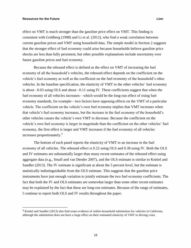
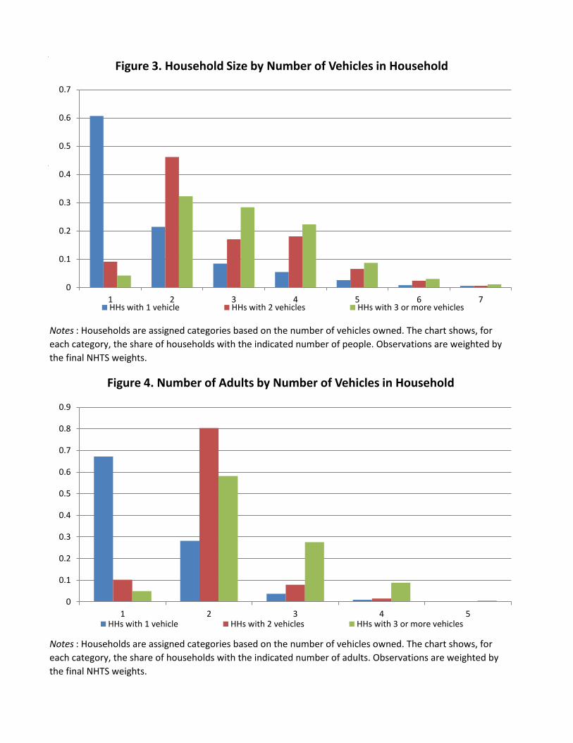
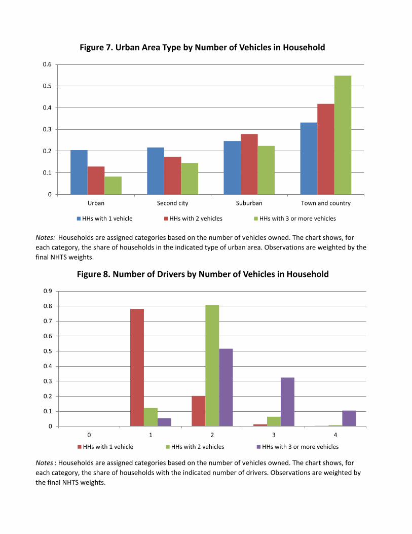
Figures 1–10 show the distributions of the categorical variables. The demographic

variables, including income, education, age of the household head, household size, number of

adults, and number of drivers, vary considerably across household types. Households with more

than two vehicles tend to have higher income, more adults, and more drivers than households

with fewer vehicles. Figures 7, 9, and 10 show that households with more vehicles also tend to

be located in more rural areas.

As noted in Section 3, one of the maintained assumptions in equation (5) is that the

current gasoline price is exogenous. Although this assumption cannot be tested directly, Table 2

shows that the current gasoline price is uncorrelated with household and geographic variables.

Each column reports a separate regression with the dependent variable indicated at the top of the

3 Because VMT is estimated for the 12 months prior to the survey, I have also used the average price over the

previous 12 months, which yields similar results.


15

table. The sample includes all observations in the final data set, and the independent variables

include sets of dummy variables for the categorical variables indicated in the table, as well as

MSA size fixed effects, urban area size fixed effects, CMSA fixed effects, and interactions of

model fixed effects with the number of vehicles belonging to the household. Observations are

weighted using the NHTS survey weights, and standard errors are clustered by state. The table

reports the p-values of F tests on the joint significance of the fixed effects for the categorical

variables. Column 1, for which the dependent variable is the log gasoline price, shows that none

of the sets of fixed effects is jointly statistically significant at conventional levels, although

household income and the number of adults are marginally significant. The results suggest that

gasoline prices are not strongly correlated with the other variables, thus supporting the

exogeneity assumption. On the other hand, the vehicle’s fuel economy (column 2) and the

average fuel economy of other vehicles owned by the household are significantly correlated with

some of the other variables. These correlations motivate the IV approach described in the

previous section and implemented in the next section.

5. Estimation Results

This section presents the main estimates of equation (5) and reports results from a variety

of alternative specifications. The baseline estimates suggest that a 1 percent increase in fuel

economy increases VMT by 0.2 to 0.4 percent. The section concludes by showing that imposing

the three assumptions described in Section 2 significantly affects the estimated rebound effect.

5.1 Main Results

Table 3 reports estimates of equation (5). The dependent variable is the log of the

vehicle’s VMT. Besides the reported variables, the regressions include the same independent

variables as in Table 2. Observations are weighted using the NHTS survey weights. Standard

errors are clustered by state.

Panel A reports the results from estimating equation (5) by OLS. Panel B is the same as

Panel A except that equation (5) is estimated by IV rather than by OLS, using as instruments the

gasoline price at the time of purchase interacted with model fixed effects.

In column 1, which I refer to as the baseline specification, both the OLS and IV estimates

show that VMT responds more than twice as much to fuel economy as to gasoline prices. The

fuel economy coefficients are statistically significant at the 5 percent level. Furthermore, the

coefficient on the gasoline price is not statistically significant, implying that the fuel economy


16

effect on VMT is much stronger than the gasoline price effect on VMT. This finding is

consistent with Goldberg (1998) and Li et al. (2012), who find a weak correlation between

current gasoline prices and VMT using household data. The simple model in Section 2 suggests

that the stronger effect of fuel economy could arise because households believe gasoline price

shocks are less than fully persistent, but other possible explanations include uncertainty over

future gasoline prices and fuel economy.

Because the rebound effect is defined as the effect on VMT of increasing the fuel

economy of all the household’s vehicles, the rebound effect depends on the coefficient on the

vehicle’s fuel economy as well as the coefficient on the fuel economy of the household’s other

vehicles. In the baseline specification, the elasticity of VMT to the other vehicles’ fuel economy

is about –0.03 using OLS and about –0.11 using IV. These coefficients suggest that when the

fuel economy of all vehicles increases—which would be the long-run effect of rising fuel

economy standards, for example—two factors have opposing effects on the VMT of a particular

vehicle. The coefficient on the vehicle’s own fuel economy implies that VMT increases when

that vehicle’s fuel economy increases, but the increase in the fuel economy of the household’s

other vehicles causes the vehicle’s own VMT to decrease. Because the coefficient on the

vehicle’s own fuel economy is larger in magnitude than the coefficient on the other vehicles’ fuel

economy, the first effect is larger and VMT increases if the fuel economy of all vehicles

increases proportionately.4

The bottom of each panel reports the elasticity of VMT to an increase in the fuel

economy of all vehicles. The rebound effect is 0.22 using OLS and 0.38 using IV. Both the OLS

and IV estimates are substantially larger than many recent estimates of the rebound effect using

aggregate data (e.g., Small and van Dender 2007), and the OLS estimate is similar to Knittel and

Sandler (2013). The IV estimate is significant at about the 5 percent level, but the estimate is

statistically indistinguishable from the OLS estimate. This suggests that the gasoline price

instruments have just enough variation to jointly estimate the two fuel economy coefficients. The

fact that both the IV and OLS estimates are somewhat larger than some other recent estimates

may be explained by the fact that these are long-run estimates. Because of the range of estimates,

I continue to report both OLS and IV results throughout the paper.

4 Knittel and Sandler (2013) also find some evidence of within-household substitution for vehicles in California,

although the substitution does not have a large effect on their estimated elasticity of VMT to driving costs.


17

5.2 Robustness of the Main Specification

I report the results of a variety of additional regressions that assess the overall robustness

of the estimates in column 1 of Table 3. Table 2 shows that the vehicle’s fuel economy is

correlated with some household characteristics. This correlation suggests that fuel economy is

not exogenous and may therefore be correlated with omitted household characteristics. The IV

approach in Panel B of Table 3 should reduce any resulting bias, but another approach is to add

further interactions between the household characteristics and vehicle characteristics. This

reduces the amount of variation available to identify the rebound effect, but it controls flexibly

for other household characteristics that may be correlated with fuel economy.

Columns 2–7 of Table 3 include triple interactions between model fixed effects, fixed

effects for the number of household vehicles, and fixed effects for the household characteristic

noted at the bottom of the table. For example, column 2 controls flexibly for any unobserved

household characteristic that varies by income level, model, and number of vehicles; this

regression allows for the possibility that driving tendencies for the Toyota Camry differ between

poor and wealthy households. Looking across the specifications, the OLS coefficients are similar

in magnitude and remain statistically significant in all cases. The point estimates in the IV

regressions are larger in some cases than the baseline estimates in column 1, but the finding of a

large rebound effect is robust. Because the coefficients are more precisely estimated in column 1,

and that specification already includes an extensive set of control variables and interaction terms,

I refer to that specification as the baseline estimates.

Table 4 shows results using alternative measures of the fuel economy of other vehicles.

As discussed above, it is straightforward to control for the fuel economy of the household’s other

vehicles for one- and two-vehicle households. In Table 3, for households with more than two

vehicles, I use the average fuel economy of the household’s other vehicles. An alternative to

using average fuel economy is to order the household’s vehicles by some criterion and control

separately for the fuel economy of those vehicles. Column 1 of Table 4 orders vehicles by VMT,

and column 2 orders vehicles by fuel economy. The samples are restricted to households with 1–

3 vehicles. For comparison with columns 1 and 2, column 3 reports the same specification as in

Table 3, except that the sample is restricted to households with 1–3 vehicles. Overall, the

rebound effect does not depend strongly on the measure of other vehicles’ fuel economy.

Table 5 allows the rebound effect to vary across vehicles or by household income.

Columns 1 and 3 report results allowing for a separate fuel economy coefficient by vehicle type.

Some evidence suggests that the rebound effect varies by vehicle type, where VMT may be more


18

responsive for SUVs than for other vehicles. Columns 2 and 4 add to the baseline specification

the interaction between the vehicle’s fuel economy and the household’s income, where income is

computed as the midpoint of the corresponding income category (see Figure 2). I find weak

evidence that households with lower income are more responsive, which is consistent with West

(2004), although the income–fuel economy interaction is not statistically significant.

5.3 Implications of Imposing Assumptions (a)–(c)

Section 2 discusses three assumptions maintained in the rebound literature. Table 6

reports versions of equation (5) that, starting from the baseline specification in Table 3, impose

these assumptions one at a time.

Assumption (a) holds that vehicle fuel economy is uncorrelated with other vehicle

characteristics. Panel A in column 1 imposes this assumption by replacing the model fixed

effects with vehicle type fixed effects and by not instrumenting for fuel economy. The estimated

rebound effect, reported at the bottom of the panel, is much smaller than that reported in column

1 of Table 3.

Assumption (b) maintains that, for a multivehicle household, VMT is independent of the

fuel economy of the household’s other vehicles. Column 2 imposes this assumption by omitting

the fuel economy of the household’s other vehicles. This specification effectively treats each

observation as unique, assuming that the fuel economy of one vehicle does not affect the VMT

of the other vehicles belonging to the household. The coefficient on fuel economy is very similar

to the baseline estimates, causing the rebound effect to be much larger when omitting the fuel

economy of other vehicles.

Finally, assumption (c) holds that the response of VMT to gasoline prices is inversely

proportional to the response to fuel economy. I impose this assumption by modifying equation

(5) in two ways. First, column 3 omits the two fuel economy variables and omits the model fixed

effects. The coefficient on gasoline prices represents the elasticity of VMT to gasoline prices,

and the estimated coefficient is much smaller than the preferred estimates of the rebound effect.

The second approach to imposing assumption (c) is to use fuel costs in place of fuel

economy, where fuel costs are the ratio of the current gasoline price to fuel economy. Column 4

implements this approach, and the specification is otherwise identical to the baseline. The


19

rebound effect is much smaller than the baseline. The results in columns 3 and 4 suggest that

rebound estimates based on regressions of VMT on gasoline prices or fuel costs underestimate

the fuel economy rebound effect.5

6. Rebound Effect for Hypothetical Fuel Economy Increases

I use the estimates from Section 5 to calculate the rebound effect from hypothetical fuel

economy increases. This analysis has two main objectives. The first is to estimate the changes in

VMT and gasoline consumption from the upcoming passenger vehicle fuel economy standards.

This analysis does not include all of the behavioral responses to standards, such as changes in

used vehicle markets and vehicle retirements, and instead focuses on the implications of the

rebound effect for estimates of future fuel savings. The second objective is to quantify the

importance of relaxing assumptions (a)–(c), which is useful for researchers making modeling

choices when estimating the welfare effects of fuel economy standards and other transportation

policies.

Table 7 reports the main results. Panel A shows the change in VMT and gasoline

consumption assuming that the fuel economy of all vehicles in the estimation sample increases

by 44 percent, which is the increase expected for the 2016 standards (US EPA 2011). This

scenario approximates the effects of fuel economy standards that raise the fuel economy of all

vehicles proportionately. By raising the fuel economy of all vehicles in the data set, including

vehicles purchased recently and those purchased many years prior to the survey, the scenario

corresponds to the long run, after the entire vehicle stock has been replaced by vehicles meeting

the new standards.

Each column shows the calculated fractional change in VMT and gasoline consumption

using the coefficient estimates from the specification indicated at the bottom of the table. For

reference, gasoline consumption would fall by 31 percent in the absence of a rebound effect.

The preferred specifications are in columns 1 and 2, which use the coefficient estimates

from column 1 of Table 3. In Table 7, column 1 reports the results based on the OLS

coefficients, and column 2 reports the results based on the IV coefficients. VMT increases by

5 Some studies define the rebound effect as the elasticity of gasoline consumption to fuel economy. An implication

of the results in Table 6 is that estimating the rebound effect using this definition but using gasoline prices or fuel

costs instead of fuel economy would lead to an underestimate of the rebound effect.


20

about 8–14 percent, and the rebound effect erodes about one-third of the gasoline savings from

the fuel economy increase; this is substantially larger than the 10 percent erosion assumed by US

EPA (2011) in the agency’s estimate of the benefits of upcoming fuel economy standards.

The remaining columns in Table 7 show the effects of imposing assumptions (a)–(c).

Column 3 shows that the rebound effect is substantially smaller when imposing assumption (a)

by omitting model fixed effects and estimating equation (5) by OLS rather than by IV. Omitting

other vehicle fuel economy—that is, imposing assumption (b)—results in a larger rebound effect,

which can be seen by comparing columns 2 and 4. Finally, columns 5 and 6 show that the

estimated rebound effect is much smaller when one imposes assumption (c), that gasoline prices

and fuel economy have equal and opposite effects on VMT.

Panel B reports the same calculations but with the assumption that the vehicles achieve

the same fuel economy increases predicted by the US EPA and National Highway Traffic Safety

Administration analysis of the 2016 fuel economy standards. This scenario may provide a more

accurate sense of future fuel economy increases than those considered in the first scenario. The

predicted fuel economy increases vary considerably across models, and this scenario allows for

the possibility that the estimated level of the rebound effect is correlated (negatively or

positively) with the predicted fuel economy increases. However, in practice, the estimated

rebound effect is not strongly correlated with the predicted fuel economy increases, and the table

shows that the results are nearly identical to those reported in Panel A (the results are similar

allowing for a heterogeneous rebound effect as in Table 5).

7. Conclusions

Rising passenger vehicle fuel economy standards in the United States and many other

countries will dramatically reduce the cost of driving. The effectiveness of the standards at

reducing fuel consumption and associated greenhouse gas emissions depends, in large part, on

the extent to which consumers increase VMT because of the lower driving costs—that is, the

magnitude of the rebound effect for passenger vehicles.

Although a substantial literature has attempted to estimate the rebound effect, the studies

have made at least one of three assumptions: (a) fuel economy is uncorrelated with other vehicle

attributes that affect the utility of driving; (b) for multivehicle households, the fuel economy of

one vehicle does not affect the VMT of another vehicle; and (c) the effect of gasoline prices on

VMT is inversely proportional to the effect of fuel economy on VMT.


21

I show that these assumptions have important implications for empirical estimates of the

rebound effect. Relaxing these assumptions implies that a 1 percent increase in the fuel economy

of all of a household’s vehicles increases VMT by 0.2 to 0.4 percent. The rebound effect erodes

about one-third of the fuel savings that would otherwise occur from rising fuel economy

standards. The rebound effect is smaller when one imposes the assumption that fuel economy is

uncorrelated with unobserved vehicle characteristics and larger when one assumes that the VMT

of one vehicle does not affect the VMT of a household’s other vehicles. The rebound effect is

smaller when one assumes that the effect of gasoline prices on VMT is equal in magnitude to the

effect of fuel economy. Future research attempting to model the effect of such standards

therefore should not impose the three assumptions.


22

References

Allcott, H., and N. Wozny. 2012. Gasoline Prices and the Fuel Economy Discount Puzzle.

NBER Working Paper 18583.

Anderson, S.T., R. Kellogg, and J.M. Sallee. 2011. What Do Consumers Believe about Future

Gasoline Prices? NBER Working Paper 16974.

Bento, A., L. Goulder, M. Jacobsen, and R. Von-Haefen. 2009. Efficiency and Distributional

Impacts of Increased US Gasoline Taxes. The American Economic Review 99(3): 667–

99.

Busse, M., C. Knittel, and F. Zettlemeyer. 2013. Are Consumers Myopic? Evidence from New

and Used Car Purchases? The American Economic Review 103(1): 220–256.

EPA (US Environmental Protection Agency) and DOT (US Department of Transportation).

2011. Draft Joint Technical Support Document: Proposed Rulemaking for 2017–2025

Light-Duty Vehicle Greenhouse Gas Emission Standards and Corporate Average Fuel

Economy Standards. EPA-420-D-11-901. Washington, DC: EPA and DOT.

Feng, Y., D. Fullerton, and L. Gan. 2005. Vehicle Choices, Miles Driven, and Pollution Policies.

NBER Working Paper 11553.

Frondel, M., N. Ritter, and C. Vance. 2012. Heterogeneity in the Rebound Effect: Further

Evidence for Germany. Energy Economics 34(2): 461-7.

Gillingham, K. 2012. Selection on Anticipated Driving and the Consumer Response to Changing

Gasoline Prices. Working paper, School of Forestry and Environmental Studies, Yale

University.

Gillingham, K. 2013. Identifying the Elasticity of Driving: Evidence from a Gasoline Price

Shock in California. Working paper, School of Forestry and Environmental Studies, Yale

University.

Gillingham, K., M. J. Kotchen, D.S. Rapson, and G. Wagner. 2013. The Rebound Effect is Over-

played. Nature 493: 475-476.

Greene, D. 2012. Rebound 2007: Analysis of National Light-Duty Vehicle Travel Statistics.

Energy Policy 41: 14-28.

Goldberg, P.K. 1998. The Effects of the Corporate Average Fuel Economy Standards in the US.

The Journal of Industrial Economics 46: 1-33.


23

Jacobsen, M. 2013. Evaluating US Fuel Economy Standards in a Model with Producer and

Household Heterogeneity. American Economic Journal: Economic Policy 5(2): 148–187.

Klier, T., and J. Linn. 2010. The Price of Gasoline and the Demand for Fuel Efficiency:

Evidence from Monthly New Vehicle Sales Data. American Economic Journal:

Economic Policy 2(3): 134–153.

Klier, T., and J. Linn. 2012. New Vehicle Characteristics and the Cost of the Corporate Average

Fuel Economy Standards. RAND Journal of Economics 43(1): 186–213.

Knittel, C., and R. Sandler. 2013. The Welfare Impact of Indirect Pigouvian Taxation: Evidence

from Transportation.

Li, S., J. Linn, and E. Muehlegger. Gasoline Taxes and Consumer Behavior. NBER Working

Paper 17891.

Small, K., and K. van Dender. 2007. Fuel Efficiency in Motor Vehicle Travel: The Declining

Rebound Effect. The Energy Journal 28(1): 25–51.

Spiller, Elisheba. 2012. Household Vehicle Bundle Choice and Gasoline Demand: A Discrete-

Continuous Choice.

West, S. 2004. Distributional Effects of Alternative Vehicle Pollution Control Policies. The

Journal of Public Economics 88: 735–757.

Figures and Tables

See following pages.

HHs with 3 or more vehicles


Notes : Households are assigned categories based on the number of vehicles owned. The chart shows, for

each category, the share of vehicles owned that are in the indicated age range. Observations are weighted by

the final NHTS weights.


each category, the share of households in the indicated income range. Observations are weighted by the final

NHTS weights.

0

0.05

0.1

0.15

0.2

0.25

0.3

< 4 years 4-6 years 6-9 years 10-13 years 13+ years

Figure 1. Vehicle Age by Number of Vehicles in Household

HHs with 1 vehicle HHs with 2 vehicles HHs with 3 or more vehicles

0

0.05

0.1

0.15

0.2

0.25

0.3

0.35

Figure 2. Income by Number of Vehicles in Household





each category, the share of households with the indicated number of people. Observations are weighted by



each category, the share of households with the indicated number of adults. Observations are weighted by


0

0.1

0.2

0.3

0.4

0.5

0.6

0.7

1 2 3 4 5 6 7

Figure 3. Household Size by Number of Vehicles in Household


0

0.1

0.2

0.3

0.4

0.5

0.6

0.7

0.8

0.9

1 2 3 4 5

Figure 4. Number of Adults by Number of Vehicles in Household





each category, the share of households with a household head achieving the indicated education level.

Observations are weighted by the final NHTS weights.


each category, the share of households with a household head in the indicated age range. Observations are

weighted by the final NHTS weights.

0

0.05

0.1

0.15

0.2

0.25

0.3

0.35

Less than high schoolgraduate

High school graduate,including GED

Some college or associate'sdegree

Bachelor's degree

Figure 5. Education Level by Number of Vehicles in Household


0

0.05

0.1

0.15

0.2

0.25

0.3

0.35

0.4

< 40 years 40-48 years 49-55 years 56-64 years 65+ years

Figure 6. Age of Household Head by Number of Vehicles in Household




Notes: Households are assigned categories based on the number of vehicles owned. The chart shows, for

each category, the share of households in the indicated type of urban area. Observations are weighted by the

final NHTS weights.


each category, the share of households with the indicated number of drivers. Observations are weighted by


0

0.1

0.2

0.3

0.4

0.5

0.6

Urban Second city Suburban Town and country

Figure 7. Urban Area Type by Number of Vehicles in Household


0

0.1

0.2

0.3

0.4

0.5

0.6

0.7

0.8

0.9

0 1 2 3 4

Figure 8. Number of Drivers by Number of Vehicles in Household





each category, the share of households in the indicated MSA size. Observations are weighted by the final

NHTS weights.


each category, the share of households with the indicated urban area size. Observations are weighted by the

final NHTS weights.

0

0.05

0.1

0.15

0.2

0.25

0.3

0.35

0.4

In an MSA of lessthan 250,000

In an MSA of250,000 - 499,999

In an MSA of500,000 - 999,999

In an MSA orCMSA of 1,000,000

- 2,999,999

In an MSA orCMSA of 3 million

or more

Not in MSA orCMSA

Figure 9. MSA Size by Number of Vehicles in Household


0

0.05

0.1

0.15

0.2

0.25

0.3

0.35

0.4

0.45

0.5

50,000-200,000 200,000-500,000 500,000-1 million >1 million withoutrail

>1 million with rail Not urbanized

Figure 10. Urban Area Size by Number of Vehicles in Household


Households with 1

vehicle

Households with 2

vehicles

Households with 3

vehicles

Households with 4+

vehicles

Population share 0.11 0.42 0.26 0.20

Share of vehicles 0.18 0.42 0.23 0.17

VMT share 0.17 0.43 0.24 0.16

10.77 12.12 12.07 11.71

(9.57) (9.79) (10.32) (10.36)

2.79 2.74 2.76 2.77

(1.02) (1.03) (1.02) (1.02)

23.80 22.53 22.00 21.44

(5.26) (5.69) (5.79) (5.68)

5.71 4.03 3.09 2.51

(6.97) (5.25) (4.42) (3.77)

2.90 1.73 1.26 0.96

(4.71) (2.75) (2.16) (1.54)

Table 1.

Summary Statistics by Number of Household Vehicles

Notes : Each household is assigned a category based on the number of vehicles it owns. For each category

indicated in the column heading, Panel A reports the population share, share of vehicles, and share of VMT

accounted for by households in the corresponding category. Shares are constructed using household weights.

Panel B reports weighted means of the indicated variables by household category with standard deviations in

parentheses.

Panel A: Shares of population, vehicles, and VMT

Panel B: Means and standard deviations

Thousand VMT

Gasoline price

($/gallon)

Thousand housing

units per sq mi

Thousand people per

sq mi

Fuel economy (mpg)

(1) (2) (3)

Gasoline price Vehicle fuel economyFuel economy of other

household vehicles

Vehicle age 0.90 0.00 0.00

Household

income0.09 0.08 0.00

Household size 0.48 0.08 0.22

Number of adults 0.07 0.03 0.36

Education 0.21 0.20 0.00

Age 0.34 0.12 0.01

Number of

drivers0.58 0.27 0.00

Table 2.

Joint Significance Tests of Categorical Variables for Gasoline Price and Fuel Economy

Regressions

Notes : Each column reports hypothesis tests based on a separate regression. The sample in each regression

includes all households in the final sample. The dependent variable is the log gasoline price in column 1, the

vehicle's fuel economy in column 2, and the log average fuel economy of the household's other vehicles in

column 3. All regressions include the same set of independent variables and have 229,851 observations.

Standard errors are clustered by state, and observations are weighted by the household sample weight. Besides

the reported variables, all regressions include fixed effects for urban category, fixed effects for MSA size, fixed

effects for urban area size, state by CMSA fixed effects, and interactions of model fixed effects by fixed effects

for the number of vehicles belonging to the household. Vehicle age uses the 5 age categories in Figure 1.

Household income uses the 18 income categories in Figure 2. Household size uses the 7 categories in Figure 3.

Number of adults uses the 5 categories in Figure 4. Education uses the 4 categories in Figure 5. Age uses the 5

age categories in Figure 6. Urban area type category uses the 4 categories in Figure 7. Number of drivers uses

the 4 categories in Figure 8. The table reports the p-values from a series of F-tests on the joint significance of

the indicated categorical variables in the corresponding regression.

(1) (2) (3) (4) (5) (6) (7)

-0.093 -0.214 -0.106 -0.092 -0.093 -0.071 -0.110

(0.085) (0.118) (0.088) (0.101) (0.089) (0.089) (0.079)

0.245 0.238 0.232 0.247 0.208 0.272 0.241

(0.044) (0.049) (0.051) (0.054) (0.055) (0.044) (0.056)

-0.029 -0.026 -0.029 -0.025 -0.027 -0.026 -0.027

(0.006) (0.005) (0.006) (0.006) (0.006) (0.005) (0.006)

R2 0.17 0.36 0.25 0.22 0.25 0.25 0.22

0.222 0.217 0.208 0.226 0.186 0.251 0.186

(0.046) (0.049) (0.052) (0.055) (0.055) (0.044) (0.055)

-0.084 -0.202 -0.091 -0.084 -0.085 -0.063 -0.099

(0.086) (0.120) (0.090) (0.103) (0.091) (0.091) (0.081)

0.473 0.532 0.626 0.633 0.542 0.685 0.515

(0.193) (0.180) (0.194) (0.190) (0.195) (0.188) (0.191)

-0.109 -0.125 -0.133 -0.086 -0.104 -0.093 -0.113

(0.027) (0.037) (0.035) (0.032) (0.035) (0.031) (0.033)

R2 0.17 0.36 0.26 0.22 0.25 0.25 0.22

0.384 0.429 0.517 0.562 0.457 0.609 0.423

(0.195) (0.178) (0.192) (0.193) (0.193) (0.194) (0.193)

Interactions

included

Model f.e. X

number of

vehicles f.e.

Column (1)

X income

group f.e.

Column (1)

X

household

size f.e.

Column (1)

X number

of adults

f.e.

Column (1)

X education

group f.e.

Column (1)

X age group

f.e.

Column (1)

X number

of drivers

f.e.

Table 3.

Effects of Fuel Prices and Fuel Economy on VMT

Notes : Each column in each panel reports a separate regression. Standard errors are reported in parentheses

and are clustered by state. The sample is the same as in Table 2. The dependent variable is the log of VMT. The

table reports coefficients on log fuel price, log fuel economy, and log of the average fuel economy of other

vehicles. Panel B reports the same specifications as Panel A, except that log fuel economy and log of other

vehicles' fuel economy are instrumented using the price of gasoline at the time of purchase interacted with a

set of model fixed effects (f.e.). All regressions include the fixed effects used in the regressions in Table 2.

Column 1 includes interactions of model fixed effects by the household's number of vehicles. Columns 27

replace these interactions with the interactions indicated at the bottom of the table. The fuel economy rebound

effect is the effect on VMT of increasing all vehcles' fuel economy by 1 percent.

Log fuel price

Log fuel economy

Log other vehicles'

fuel economy

Log fuel price

Log fuel economy

Log other vehicles'

fuel economy

Fuel economy

rebound effect

Fuel economy

rebound effect

Panel A: OLS

Panel B: IV

(1) (2) (3)

-0.154 -0.156 -0.093

(0.119) (0.119) (0.119)

0.324 0.338 0.256

(0.078) (0.078) (0.063)

-0.023

(0.006)

-0.087 -0.124

(0.028) (0.046)

-0.030 -0.007

(0.031) (0.047)

-0.155 -0.110

(0.055) (0.075)

R2 0.16 0.16 0.16

-0.154 -0.157 -0.087

(0.119) (0.119) (0.119)

0.549 0.522 0.555

(0.257) (0.276) (0.223)

-0.113

(0.041)

-0.114 -0.153

(0.034) (0.068)

-0.051 -0.014

(0.045) (0.044)

-0.176 -0.126

(0.055) (0.078)

R2 0.16 0.16 0.16

Specification Rank other vehicles by VMTRank other vehicles by fuel

economy

Include households with 1-3

vehicles

Table 4.

Alternative Measures of Other Vehicles' Fuel Economy

Panel A: OLS

Log fuel price

Log fuel economy

Log other vehicles'

fuel economy

Panel B: IV

Log fuel price

Log other vehicles'

fuel economy


and are clustered by state. Except as indicated, the specifications in Panel A are identical to the specification in

column 1 of Panel A of Table 3 and the specifications in Panel B are identical to that in column 1 of Panel B of

Table 3. Columns 1 and 2 replace the log of other vehicles' average fuel economy with the fuel economy of

each of the other vehicles and include households with 1-3 vehicles. For column 1, vehicles are ranked in order

of decreasing miles traveled, so that vehicle 1 has the highest miles traveled of vehicles owned by the

household. Column 2 is similar, ranking vehicles by fuel economy rather than miles traveled. Column 3 repeats

the specification from Table 3 except that the sample includes households with 1-3 vehicles.

Log fuel economy

vehicle 1

Log fuel economy

vehicle 2

Log fuel economy

vehicle 3

Log fuel economy

vehicle 1

Log fuel economy

vehicle 2

Log fuel economy

vehicle 3

Log fuel economy

(1) (2) (3) (4)

-0.095 -0.093 -0.090 -0.089

(0.084) (0.085) (0.086) (0.086)

0.244 0.474

(0.044) (0.190)

0.247 0.444

(0.050) (0.195)

0.222 0.784

(0.057) (0.279)

0.300 0.917

(0.055) (0.219)

0.230 0.699

(0.062) (0.296)

-0.010 0.250

(0.022) (0.163)

-0.029 -0.029 -0.111 -0.100

(0.006) (0.006) (0.029) (0.026)

R2 0.17 0.17 0.17 0.17

Regression

estimated byOLS OLS IV IV

Table 5.

Fuel Economy Interacted with Vehicle Type and Income

Log fuel price

Log fuel economy

Log fuel economy X

log income

Notes : Each column reports a separate regression. Standard errors are reported in parentheses and are

clustered by state. Except as indicated, the specifications are identical to the specification in column 1 of Panel B

of Table 3. Column 1 includes the interactions between the log fuel economy and a set of fixed effects for the

vehicle type. Column 2 includes the log of fuel economy interacted with the log of household income, which is

estimated as the midpoint of the corresponding income group. Columns 3 and 4 are identical to columns 1 and

2 except that they are estimated by IV rather than by OLS, using the same instruments as in Table 3.

Log fuel economy X

SUV

Log fuel economy X

pickup

Log fuel economy X

car

Log fuel economy X

van

Log other vehicles'

fuel economy

(1) (2) (3) (4)

-0.114 -0.096 -0.119

(0.101) (0.085) (0.100)

0.129 0.247

(0.031) (0.044)

-0.031

(0.006)

-0.200

(0.042)

0.007

(0.007)

R2 0.12 0.17 0.11 0.17

0.104 0.247 0.194

(0.032) (0.044) (0.043)

-0.104 -0.097

(0.101) (0.085)

0.284 0.476

(0.076) (0.194)

-0.154

(0.038)

-0.094

(0.081)

-0.066

(0.027)

R2 0.12 0.17 0.17

0.159 0.476 0.148

(0.084) (0.194) (0.073)

SpecificationOmit model fixed

effects

Omit other vehicle

fuel economy

Include only current

gasoline price

Replace fuel

economy with fuel

costs

Fuel economy

rebound effect

Fuel economy

rebound effect

Table 6.

Rebound Effects without Relaxing Assumptions (a) - (c)

Panel A: OLS


and are clustered by state. Regressions in Panel A are estimated by OLS, and regressions in Panel B are

estimated by IV using the same instruments as in Table 3. The specifications are the same as in Table 3 except as

indicated. Column 1 replaces model fixed effects with vehicle type fixed effects. Column 2 omits the fuel

economy of the household's other vehicles. Column 3 omits fuel economy and other vehicle fuel economy.

Column 4 omits the log fuel price and replaces fuel economy with fuel costs. The fuel economy rebound effect is

computed as in Table 3.

Log fuel price

Log fuel economy

Panel B: IV

Log fuel price

Log fuel economy

Log other vehicles'

fuel economy

Log other vehicles'

fuel economy

Log fuel costs

Log other vehicle

fuel costs

Log fuel costs

Log other vehicle

fuel costs

(1) (2) (3) (4) (5) (6)

VMT (fractional change) 0.09 0.15 0.04 0.19 0.04 0.06

Gas consumption

(fractional change)-0.25 -0.20 -0.28 -0.18 -0.28 -0.27

VMT (fractional change) 0.09 0.16 0.04 0.19 0.05 0.06

Gas consumption

(fractional change)-0.25 -0.21 -0.29 -0.18 -0.28 -0.27

Specification used for

simulations

Baseline, OLS

(Table 3,

column 1,

Panel A)

Baseline, IV

(Table 3,

column 1,

Panel B)

Omit model

fixed effects

(Table 6,

column 1,

Panel A)

Omit other

vehicle fuel

economy

(Table 6,

column 2,

Panel B)

Gas price

coefficient

(Table 6,

column 3,

Panel A)

Fuel costs

(Table 6,

column 4,

Panel B)

Notes : Each column in each panel reports a separate simulation. Panel A simulates miles traveled and gasoline

consumption assuming the fuel economy of every vehicle increases 44 percent. Panel B assumes each vehicle's

fuel economy increases by the amount predicted by US EPA (2011). Assuming no rebound effect, both scenarios

would reduce gasoline consumption by about 31 percent. Each column uses the regression results from the

specification indicated at the bottom of the table. The table reports the fractional change in VMT and gas

consumption using the estimated coefficients and comparing the miles traveled and gasoline consumption in

the 2009 NHTS with the counterfactual miles traveled and gasoline consumption under the fuel economy

increases.

Table 7.

Effect of Increasing Fuel Economy on VMT and Gasoline Consumption

Panel A: 44% Fuel economy increase

Panel B: Predicted 2016 CAFE fuel economy increases

Documents

The Rebound Effect for Passenger Vehicles - rff.org · 1616 P St. NW Washington, DC 20036 202-328-5000 July 2013 RFF DP 13-19 The Rebound Effect for Passenger Vehicles DISCUSSION