Embed Size (px)
Citation preview
NASA/CRm1998 -208537
The Real-Time Wall Interference Correction System of the
NASA Ames 12-Foot Pressure Wind Tunnel
Norbert Ulbrich
VERIDIAN/Calspan Operations
NASA Ames Research Center
P.O. Box 7
Moffen Field, California 94035-0007
National Aeronautics and
Space Administration
Ames Research Center
Moffett Field, California 94035-1000
Prepared for Ames Research Centerunder Contract NAS2-13605
July 1998
https://ntrs.nasa.gov/search.jsp?R=19980223963 2019-05-10T07:34:43+00:00Z
Available from:
NASA Center for AeroSpace Information7121 Standard Drive
Hanover, MD 21076-1320
(301) 621-0390
National Technical Information Service
5285 Port Royal Road
Springfield, VA 22161(703) 487-4650
PREFACE
During the past two years, substantial progress was made in the procedure and soft-
ware development of a real-time Wall Interference Corrections System (WICS) for the
NASA Ames 12ft Pressure Wind Tunnel. Experimental data became available to verify
the WICS procedures. Expert System-like diagnostic features were added to the software
to allow a reliable real-time operation. Wall interference corrections were successfully
computed for a wide variety of wind tunnel models.
I hope that the promising results obtained during the development of WICS will
benefit attempts to improve data quality and efficiency of subsonic wind tunnel tests in
the NASA Ames 12ft Pressure Wind Tunnel.
I wish to express my appreciation to Alan Boone, test engineer at NASA Ames Re-
search Center. His dedication, his extensive experience in wind tunnel testing, and his
helpful comments were critical during the facility prototype development of WICS. Recent
progress would not have been possible without his knowledge of classical wall interference
corrections and pressure measurement techniques.
I want to thank John Day and Sylvie Faisant for their contributions. Thanks also go
to Pat Whittaker, Larry Erickson, Jules Gustie, Darrell Kirk, Bob Gisler, Morgan Wright,
Jon Bader, Karlin Roth, Kevin James, Dan Petroff, Dan Clasen, Diarme Butler, Norm
Struzynski, Steve Culp, Richard Millington, Tom Bridge, Amit Ghosh, Linda Thompson,
and the staff of the Aeronautical Test and Simulation Division at NASA Ames Research
Center. I would also like to acknowledge the support from Mat Rueger, Abdi Khodadoust,
Pat Driscoll, Pete Minor, and Don Leopold of the Boeing Company.
Moffett Field, California
May 1998
Norbert Ulbrich
iii
iv
ABSTRACT
An improved version of the Wall Signature Method was developed to compute wall
interference effects in three--dimensional subsonic wind tunnel testing of aircraft models in
real-time. The method may be applied to a fullspan or a semispan model.
A simplified singularity representation of the aircraft model is used. Fuselage, support
system, propulsion simulator, and separation wake volume blockage effects are represented
by point sources and sinks. Lifting effects are represented by semi-infinite line doublets.
The singularity representation of the test article is combined with the measurement of wind
tunnel test reference conditions, wall pressure, lift force, thrust force, pitching moment,
roiling moment, and precomputed solutions of the subsonic potential equation to determine
first order wall interference corrections.
Second order wall interference corrections for pitching and rolling moment coefficient
are also determined. A new procedure is presented that estimates a rolling moment coef-
ficient correction for wings with non-symmetric lift distribution.
Experimental data obtained during the calibration of the Ames Bipod model support
system and during tests of two semispan models mounted on an image plane in the NASA
Ames 12ft Pressure Wind Tunnel are used to demonstrate the application of the wall
interference correction method.
V
vi
TABLE OF CONTENTS
CHAPTER PAGE
1. INTRODUCTION ........................... 1
2. WALL INTERFERENCE CORRECTION PREDICTION .......... 5
2.1 Definition of Interference Corrections ................. 5
2.2 Panel Method Code Solution .................... 8
2.3 Fullspan Model .......................... 10
2.3.1 Test Article Wall Interference Correction ............. 10
2.3.2 Support System Wall Interference Correction ........... 14
2.4 Semispan Model .......................... 15
2.5 Compressibility Effects ....................... 16
2.6 Normalized Perturbation Velocity Definition .............. 18
3. APPLICATION OF THE METHOD TO WIND TUNNEL TESTS ...... 23
3.1 Real-Time Wall Interference Calculation ............... 23
3.2 Matching Conditions ........................ 24
3.3 Application of the Method to Semispan Models ............ 26
3.4 Application of the Method to the Ames Bipod ............. 30
4. CONCLUSION AND REMARKS .................... 33
REFERENCES .............................. 35
APPENDICES ............................... 39
1. Higher Order Correction Formulae .................. 39
2. Panel Method Code Modifications .................. 43
3. Point Source Velocity Vector ..................... 49
4. Line Doublet Velocity Vector .................... 51
5. Calculation of the Line Doublet Strength ............... 57
6. Tri-linear Interpolation ....................... 61
7. Parabolic Interpolation ....................... 63
8. Optimization of the Singularity Location ............... 65
9. Selection of the Singularity / Reference Point Location ......... 67
10. Blockage Effects of a Powered Wind Tunnel Model ........... 71
vii
CHAPTER PAGE
11. Quality Check of the Least Squares Fit ................ 73
12. Linear Interpolation of Wall Pressure Port Calibration ......... 75
13. Singular Value Decomposition .................... 77
14. Support System Kinematics ..................... 79
15. High Angle of Attack Sting Kinematics ................ 83
16. Pitching Moment Lever Arm ..................... 87
17. Inclination of Force and Moment Vectors • .............. 91
18. Pitching Moment Coefficient Correction ................ 95
19. Rolling Moment Coefficient Correction ............... 101
20. Scale Factor Law ......................... 111
FIGURES ................................ 113
ooo
Vlll
A
a
b
C
C
C
ct
CD
ACD
cl
Cl,c
Cl,un, c
/X.cz
AW
CL
CL(y)
4
Acz
CM
CM,c
CM,unc
ACM1
ACM2
Cn
Cn,c
Cr$,_r_c
LIST OF SYMBOLS
cross-sectioni area of the wind tunnel
speed of sound
wing span
wil pressure port calibration
interpolated wall pressure port calibration
wing chord
mean aerodynamic chord (2/S. f:12 c2 dy)
mean geometric chord (S/b)
drag coefficient
uncorrected drag coefficient
drag coefficient correction due to inclination of lift and drag force
rolling moment coefficient
corrected rolling moment coefficient
uncorrected rolling moment coefficient
rolling moment coefficient correction (non-symmetric lift distribution)
rolling moment coefficient correction (inclination of moment vectors)
lift coefficient
local lift coefficient
uncorrected lift coefficient
lift coefficient correction due to inclination of lift and drag force
pitching moment coefficient
corrected pitching moment coefficient
uncorrected pitching moment coefficient
pitching moment coefficient correction due to difference between mean and
loci wil interference corrections along the 3/4-chord of the wing and tail
pitching moment coefficient correction due to streamline curvature
yawing moment coefficient
corrected yawing moment coefficient
uncorrected yawing moment coefficient
ix
A-_-d.
cp
D
D'
k
L
L'
L,
L_
l
M
M_!
Moo
m
N
n
nt
nw
P
P
P_mp
Pst_p
Ptun
PT
q
qe
q,'e!
q_
R
yawing moment coemcient correction (inclination of moment vectors)
specific heat ; pressure coefficient
drag force
uncorrected drag force
camber of circularly cambered airfoil
singularity index
lift force
uncorrected lift force
lift force of a line doublet of the tail
lift force of a line doublet of the wing
length of a Rankine body
Mach number or number of reference points
calibrated Mach number
test section reference Mach number
free-stream Mach number
number of wall pressure orifices
number of reference points
number of singularities
number of line doublets of the tail
number of line doublets of the wing
pitching moment
static pressure
static pressure at a wall orifice ; empty tannel calibration
static pressure at a wall orifice ; support system calibration
static pressure at a wall orifice ; real-time wind tunnel test
total pressure in the settling chamber
dynamic pressure
calibrated dynamic pressure
test section reference dynamic pressure
free-stream dynamic pressure
gas constant or rolling moment
X
R !
rl _ r2
ro
S
S
$
As
Ast
Asw
T
Tp
TT
U
U_
u;
U_
II
Ui
Ui
"Urn
_m
i
_s
i
_t
Ut
_t
_ts
U
Vi
uncorrected rolling moment
polar coordinate
radius of a hMfbody
area of the propeller disc of a propulsion simulator
reference area of test article
span of a rectangular wing
span of a horseshoe vortex
discrete span of a line doublet of the tail
discrete span of a line doublet of the wing
temperature
propulsion simulator thrust
total temperature in the settling chamber
velocity in the x-direction
calibrated axial velocity; empty tunnel or image plane
calculated value of u_
test section reference velocity
free--stream velocity
perturbation velocity in the x-direction
streamwise velocity correction
normalized perturbation velocity of the wM1 interference flow field ; x-component
axial perturbation velocity; model in free-air
calculated value of u,_
axial perturbation velocity; support system in free-air
normalized perturbation velocity of the wind tunnel flow field ; x-axis
axial perturbation velocity; wind tunnel flow field
calculated value of ut
axial perturbation velocity of a model in the wind tunnel flow field
axial perturbation velocity of a support system in the wind tunnel flow field
x'-axis component of the velocity vector
flow velocity in the y-direction
velocity correction in the y-direction
xi
Vi
_t
D e
¢s
Dm
_s
D s
J
Dtm
t*
D t
W
Wi
W e
W m
W 8
W_
W_
wj
Ww
Ww
W t
X
X"
X
_z
X_r
ZS
X_
Xw
X_
normalized perturbation velocity of the wall interference flow field ; y-axis
y-component of the velocity; empty tunLel or image plane calibration
y-component of the perturbation velocity; model in free-air
y-component of the perturbation velocity; support system in free-air
y-component of the perturbation velocity; model in wind tunnel flow field
y-component of the perturbation velocity; support system in wind tunnel flow field
yr-axis component of the velocity vector
flow velocity in the z-direction ; reference point weight
velocity correction in the z-direction
normalized perturbation velocity of the wall interference flow field ; z-axis
z-component of the velocity; empty tunnel or image plane calibration
z-component of the perturbation velocity; model in free--air
z-component of the perturbation velocity; support system in free-air
z-component of the perturbation velocity; model in wind tunnel flow field
z-component of the perturbation velocity; support system in wind tunnel flow field
weight of a line doublet of the tail
weight of a singularity
weight of a line doublet of the wing (syn'_metric lift distribution)
weight of a line doublet of the wing (non-symmetric lift distribution)
z'-axis component of the velocity vector
value of first calibration variable during calibration
value of first calibration variable during real-time test
x-coordinate; roll axis; line doublet starting point
pitching moment arm
incompressible x-coordinate
x-coordinate of the pitching moment reference axis
x-coordinate
x-coordinate
x-coordinate
x-coordinate
x-coordinate
of a point source
of a line doublet of the tail
of a line doublet of the wing
of a point source or line doublet starting point
of a point sink
xii
Xs
Xo
X /
Y
yt
y*
Y
yz
ys
yt
Z
Zl
ZS
Z t
x-coordinate of axis of rotation
stagnation point distance ; initial x-coordinate of singularity
x-coordinate of the reference coordinate system
value of second calibration variable during calibration or yawing moment
uncorrected yawing moment
value of second calibration variable during real-time test
y-coordinate; pitch axis
incompressible y-coordinate
y-coordinate of a line doublet starting point
y-coordinate of a point source
y-coordinate of the reference coordinate system
z-coordinate; yaw axis
incompressible z-coordinate
z-coordinate of a line doublet starting point
z-coordinate of a point source
z-coordinate of the reference coordinate system
O_rn
O_s
O_t
_oo
Z
1-'
F_
angle of attack of test article
angle of attack correction
mean angle of attack correction along 1/4-chord line of wing
mean angle of attack correction along 3/4-chord line of wing
angle of attack correction caused by the model
angle of attack correction caused by the support system
geometric angle of attack
pitch angle of High Angle of Attack Sting
free--stream angle of attack
x/1 - M 2 or sideslip angle of test article
yaw angle of High Angle of Attack Sting
circulation of a horseshoe vortex in [m 2/sec] or [ft 2/sec]
circulation constant of the tail in [m 2/sec] or [ft 2/sec]
circulation constant of the wing in [m 2/sec] or [ft 2/sec]
ooo
Xlll
##
r**
7
6
_r_in
_rn
_s
_7
0
A
!/
P
Prey
PT
P_
O"
Ork
o"I,
O"t
or w
ffl _0"2
T
_oo.2s
circulationof symmetric liftdistributionin [m2/sec] or [ft2/sec]
circulationof non-symmetric liftdistributionin [m 2/sec] or [ft2/sec]
isentropicexponent
wall pressure orificeindex
blockage factor
mean blockage factor
minimum of blockage factor
blockage factorcaused by a model
blockage factorcaused by a support system
number of source / sink pairs ;solidvolume blockage
test sectionreference point
aspect ratio of wing
model referencepoint index
number of sources and sinks
density
test sectionreference density
totaldensity in the settlingchamber
free-stream density
singularity strength in [m3/sec] or [fta/sec]
singularity strength divided by reference velocity ; [m 2] or [ft 2]
sink strength of the propulsion simulator divided by reference velocity
sink strength of the propulsion simulator in [ma/sec] or [fta/sec]
strength of a line doublet of tail divided by reference velocity
strength of a line doublet of the tail in [mZ/sec] or [ftZ/sec]
wake source strength or strength of a line doublet divided by reference velocity
wake source strength or strength of a line doublet in [m a/sec] or [ftZ/sec]
strength of a line doublet in [ma/sec] or [fta/sec]
singularity strength of a point source or sink
line doublet orientation angle ; identical with _,
roll angle of test article _ sweep angle of wing
sweep angle of 1/4-chord line of wing
xiv
_0.50
T*
eL
CPD
Cs
¢,
Coo
¢1, ¢2
sweep angle of 1/2-chord line of wing
line doublet orientation angle ; identical with r
polar coordinate
line doublet potential
point doublet potential
point source potential
wall / support system potential
wind tunnel potential
singularity potential
free-stream potential
length scale of wind tunnel model
n
uoo
Woo
normal vector at a panel centroid
free-stream velocity vector
unit wind vector in model coordinate system
XV
xvi
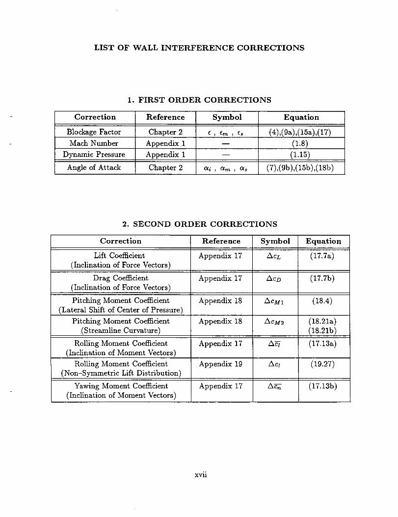
LIST OF WALL INTERFERENCE CORRECTIONS
1. FIRST ORDER CORRECTIONS
Correction Reference Symbol Equation
Blockage Factor Chapter 2 (4),(ga),(15a),(17)Mach Number Appendix 1 -- (1.8)
Dynamic Pressure Appendix 1 -- (1.15)
Angle of Attack O_i _ O_rn j _sChapter 2 (7),(9b),(15b),(18b)
2. SECOND ORDER CORRECTIONS
Correction Reference Symbol Equation
Lift Coefficient Appendix 17 ACL (17.7a)
(Inclination of Force Vectors)
Drag Coefficient Appendix 17 ACD (17.7b)
(Inclination of Force Vectors)
Pitching Moment Coefficient Appendix 18 ACM1 (18.4)
(Lateral Shift of Center of Pressure)
Pitching Moment Coefficient
(Streamline Curvature)
Appendix 18 ACM2 (18.21a)
(18.215)
Rolling Moment Coefficient Appendix 17 A_ (17.13a)
(Inclination of Moment Vectors)
Rolling Moment Coefficient Appendix 19 Act (19.27)
(Non-Symmetric Lift Distribution)
Yawing Moment Coefficient Appendix 17 AF_ (17.13b)
(Inclination of Moment Vectors)
xvii
xviii
CHAPTER1
INTRODUCTION
Wind tunnel tests have always played an important role in the development of mod-
ern aircraft. These tests are used to simulate atmospheric conditions experienced by an
aircraft or spacecraft in free-flight. Aerodynamic forces and moments are measured and
related to corresponding free flight values using Mach and Reynolds numbers. These mea-
surements provide valuable information about expected performance, stability, and control
characteristics of a new aircraft design.
Large wind tunnel models, i.e. wing span on the order of 80% of the wind tunnel
width, are often preferred in order to achieve a good simulation of viscous phenomena of
the flow field. In this case, however, the presence of the wind tunnel wall and model support
system change the free-air flow field experienced by the aircraft model. These flow field
interference effects have to be considered to allow a reasonable comparison between wind
tunnel test and free flight condition. Therefore, interference corrections to Mach number,
dynamic pressure, and angle of attack have to be determined to improve test data quality.
In the 1970s and 1980s, techniques were developed that use boundary measurements
during a wind tunnel test to predict wall interference corrections. The Wall Signature
Method introduced by Hackelt et al. [1],[2],[3] and the Two-Variable Method introduced
by Ashill [4],[5] were used extensively in 3-dimensional wind tunnel testing. Ashill [5] gives
a detailed discussion and comparison of these techniques.
The Wall Signature Method and Two-Variable Method are both based on potential
flow theory. Computed wall interference corrections agree if each method is applied cor-
rectly. However, a few differences exist between these two methods. Each method has its
advantages and disadvantages. Table 1 compares important features of the Wall Signature
Method and the Two-Variable Method.
The Two-Variable Method does not require a singularity representation of the wind
tunnel model to determine wall interference corrections. However, the wall interference
correction calculation depends on an integration of the measured and interpolated surface
pressure distribution on the wind tunnel wall.
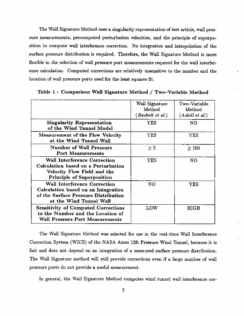
The Wall Signature Method uses a singularity representation of test article, wall pres-
sure measurements, precomputed perturbation velocities, and the principle of superpo-
sition to compute wall interference correction. No integration and interpolation of the
surface pressure distribution is required. Therefore, the Wall Signature Method is more
flexible in the selection of wall pressure port measurements required for the wall interfer-
ence calculation. Computed corrections are relatively insensitive to the number and the
location of wall pressure ports used for the least squares fit.
Table 1 : Comparison Wall Signature Method / Two-Variable Method
Wall Signature Two-Variable
Method Method
(Ita,:kett et al.) (Ashill et at.)
Singularity Representation YES NOof the Wind Tunnel Model
Measurement of the Flow Velocity YES YESat the Wind Tunnel Wall
Number of Wall Pressure ___2 >_ 100
Port Measurements
YES NOWall Interference Correction
Calculation based on a Perturbation
Velocity Flow Field and the
Principle of Superposition
Wall Interference Correction
Calculation based on an Integrationof the Surface Pressure Distribution
at the Wind Tunnel Wall
Sensitivity of Computed Corrections
to the Number and the Location of
Wall Pressure Port Measurements
NO
LOW
YES
HIGH
The Wall Signature Method was selected for use in the real-time Wall Interference
Correction System (WICS) of the NASA Ames 12ft Pressure Wind Tunnel, because it is
fast and does not depend on an integration of a measured surface pressure distribution.
The Wall Signature method will still provide corrections even if a large number of wall
pressure ports do not provide a useful measurement.
In general, the Wall Signature Method computes wind tunnel wall interference cor-
rections by introducing a simplified representation of the test article expressedin terms
of singularities. Sourcesand sinks represent the fuselagevolume and viscous separation
wake blockageeffectsand horseshoevortices or line doublets representthe lifting effects.
In addition, power simulator blockageeffectscan be representedby a sink [6] . This sin-
gula_ity representation is combinedwith a least squaresfit of wall pressuremeasurements,
data from calibration tests, and solutions of the subsonicpotential equation, in the form of
normalized perturbation velocities, to predict Mach number, dynamic pressure,and angle
of attack corrections.
During the past decadesignificant advancesin the developmentof low-order panel
method codes and computer hardware have made a fast calculation of complex three-
dimensional internal flow field problems on workstation type computers possible. Panel
method codesallow application of the Laplace Equation to realistic three--dimensionalwind
tunnel geometrieswhich is important if the methodology of the Wall Signature Method is
applied to the quasi-octogonal cross-sectionof the 12ft PressureWind Tunnel (PWT) at
NASA Ames Research Center. It was shown by Ulbrich and S_einle [7],[8] that normalized
panel method code solutions of the wind tunnel flow field combined with the Wall Signature
Method can be used to predict subsonic wall interference corrections close to real-time.
The revised formulation of the Wall Signature Method developed for the 12ft PWT is
described in detail in this report. Figure 1 shows principle elements of the modified Wall
Signature Method. Improvements of the Wall Signature Method were introduced to allow
an application of the Wall Signature Method in real-time and to deal efficiently with a
wide range of model and support system geometries.
Originally, Hacke_t et al. [1] based their formulation of the Wall Signature Method on
a "local" least squares fit procedure. They introduced a piecewise approximation of the
wall signature using a parabola for its maximum and a tanh - function for its downstream
asymptote. The location of singularities was found by matching the location of the maxi-
mum of the parabola with the inflection point of the tanh - function. Unfortunately, this
feature of the original formulation of the Wall Signature Method is difficult to use in a
real-time correction system, as it requires the selection of wall pressure ports used for the
"local" least squares fit of the maximum of the real-time wall signature.
Ulbrich [9] introduced improvements to the Wall Signature Method to overcome the
3
limitations of a "local" least squares fit of the wall pressure signature. He suggested a
"global" least squares fit procedure which matches the wall signature on all wall pressure
ports using panel method code solutions of singularities placed inside the wind tunnel test
section. In his approach, a "best" singularity location is found by minimizing the standard
deviation of the least squares fit of the wall signature as a function of the singularity
location.
Support system wall interference corrections for fullspan model tests can also be found
by applying the Wall Signature Method. In this case the Wall Signature Method has to be
applied to the difference between the support system and the empty tunnel calibration at
the wall pressure ports. Support system wall interference effects can be computed off-line
and stored in a database.
In the first part of this report, basic relationships of the proposed Wall Signature
Method are derived for a fullspan and a semispan model.
The second part of this report discusses the integration of the method into a wind tun-
nel facility. Experimental data, obtained during tests of two different size semispan models
mounted on an image plane in the NASA Ames 12ft Pressure Wind Tunnel (PWT), are
applied to the modified Wall Signature Method to verify computed corrections. Exper-
imental data recorded during the calibration of the Ames Bipod are also applied to the
method.
4
CHAPTER 2
WALL INTERFERENCE CORRECTION PREDICTION
2.1 Definition of Interference Correction
Wind tunnel tests allow the prediction of aerodynamic forces and moments acting
on an aircraft model in atmospheric free-flight. Unfortunately, the wind tunnel wall and
the model support system change the flow field experienced by the aircraft. Many of
these changes can be ignored if the aircraft model is small compared to the wind tunnel
height and width. However, if the span of the test article is large or if substanial flow
separation occurs, wall and model support system interference effects cannot be neglected.
Then, reliable estimates of interference corrections to Mach number, dynamic pressure,
and angle of attack are necessary so that wind tunnel test data may be compared with
free-flight conditions.
In general, wall and support system interference corrections are defined as the dif-
ference between the wind tunnel flow field and the free-air flow field experienced by the
model (see Fig.2a) . Corrections are described in terms of a blockage factor e and an angle
of attack correction _i . Mach number and dynamic pressure corrections are related to the
blockage factor computed at some reference point in the wind tunnel. For more detail on
classical subsonic wall interference corrections, see AGARDograph 109, [10] . The block-
age correction relates the free--stream velocity Uoo to a calibrated empty tunnel velocity
Ue at a model reference point v (see Fig. 2b) . The calibrated empty tunnel velocity Ue
captures the effects of the wind tunnel wall boundary layer growth, wall divergence, and
orifice error. It is still necessary to correct for the wall interference effect of the test article,
its separation wake, and the influence of the support system.
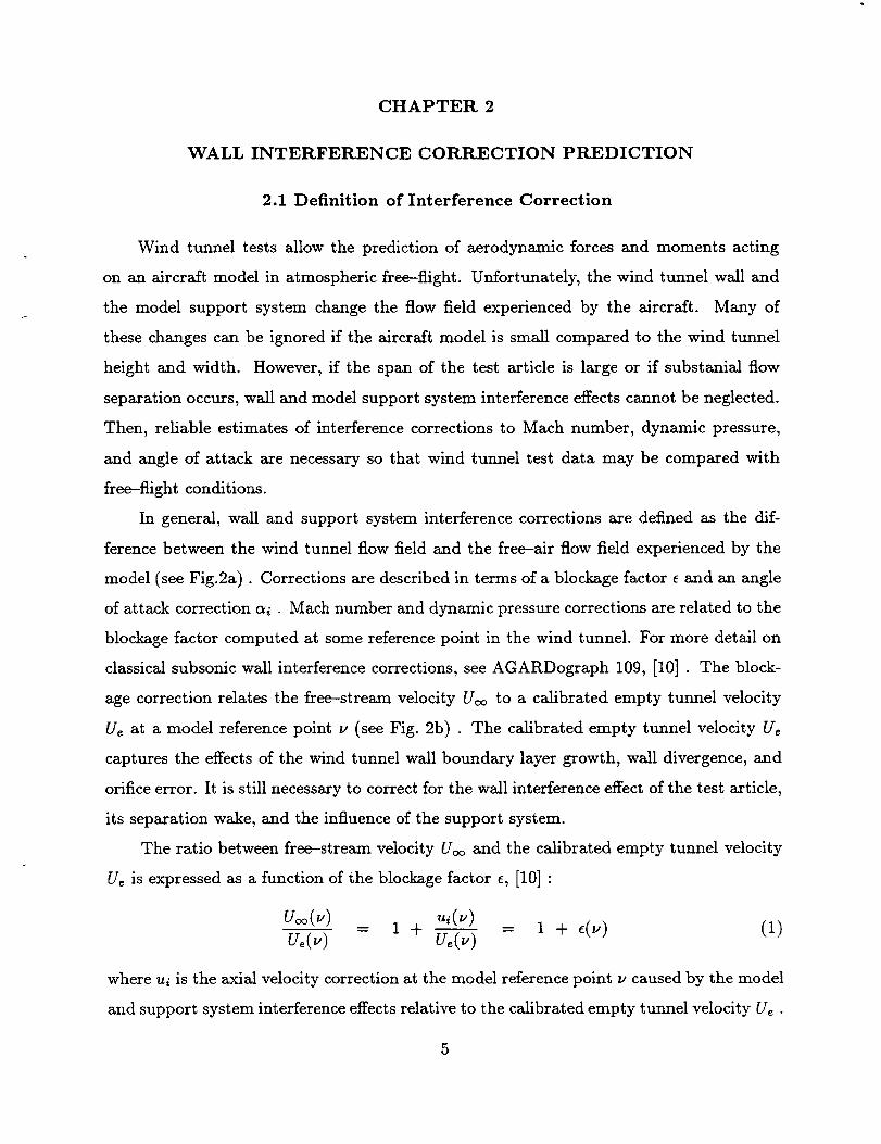
The ratio between free-stream velocity Uoo and the calibrated empty tunnel velocity
U, is expressed as a function of the blockage factor e, [10] :
Uoo(u) = 1 + ui(u) = 1 + e(u) (1)
where ui is the axial velocity correction at the model reference point u caused by the model
and support system interference effects relative to the calibrated empty tunnel velocity Ue •
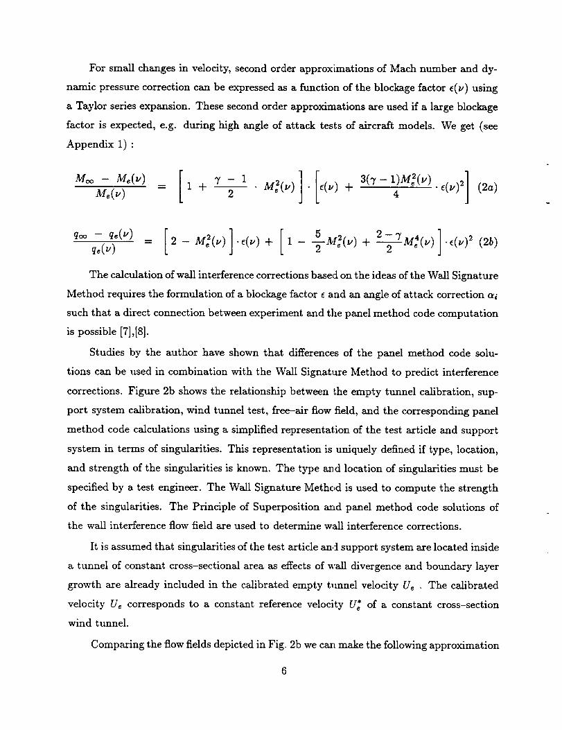
For small changes in velocity, second order approximations of Mach number and dy-
namic pressure correction can be expressed as a function of the blockage factor e(v) using
a Taylor series expansion. These second order approximations are used if a large blockage
factor is expected, e.g. during high angle of attack tests of aircraft models. We get (see
Appendix 1) :
Me(v) = 1 -{- 2 4 " e(v)2 (2a)
qoo - q_(v)=q,(v) [2- M2(v)].e(v)+ [1- -_-M_(v)+ 2-TM4(v)2 ] "e(v)2 (2b)
The calculation of wall interference corrections based on the ideas of the Wall Signature
Method requires the formulation of a blockage factor e and an angle of attack correction c_i
such that a direct connection between experiment and the panel method code computation
is possible [7],[8].
Studies by the author have shown that differences of the panel method code solu-
tions can be used in combination with the Wall Signature Method to predict interference
corrections. Figure 2b shows the relationship between the empty tunnel calibration, sup-
port system calibration, wind tunnel test, free-air flow field, and the corresponding panel
method code calculations using a simplified representation of the test article and support
system in terms of singularities. This representation is uniquely defined if type, location,
and strength of the singularities is known. The type and location of singularities must be
specified by a test engineer. The Wall Signature Method is used to compute the strength
of the singularities. The Principle of Superposition arid panel method code solutions of
the wall interference flow field are used to determine wall interference corrections.
It is assumed that singularities of the test article an,_ support system are located inside
a tunnel of constant cross-sectional area as effects of wall divergence and boundary layer
growth are already included in the calibrated empty tlmnel velocity Us . The calibrated
velocity U_ corresponds to a constant reference velocity U_ of a constant cross-section
wind tunnel.
Comparing the flow fields depicted in Fig. 2b we caz_ make the following approximation
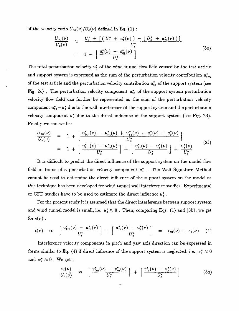
of the velocity ratio U_(v)/U_(v) defined in Eq. (1):
u_(_) u; + [( u; + u;(.) ) - ( u; + u;,(.) )]v_O,) u;
- u=(_) ]= 1 + r/i,;(,,,)L u;'
(3a)
The total perturbation velocity u_ of the wind tunnel flow field caused by the test article
and support system is expressed as the sum of the perturbation velocity contribution u_, n
of the test article and the perturbation velocity contribution u_*, of the support system (see
Fig. 2c) . The perturbation velocity component u_s of the support system perturbation
velocity flow field can further be represented as the sum of the perturbation velocity
component u_s - u_ due to the wall interference of the support system and the perturbation
velocity component u_ due to the direct influence of the support system (see Fig. 2d).
Finally we can write :
u_(_)u_(_)
r - ,-,*(,,)+,-,;.(,-,)-,,:,:,,.,,)+,-,:(,-,)1 + L u; J
= 1+ [';"'(')-07 _';'(') ]+ [ ,.,7,,(,,)57-,,i(,..')]+ ";(')U;(3b)
It is difficult to predict the direct influence of the support system on the model flow
field in terms of a perturbation velocity component us* . The Wall Signature Method
cannot be used to determine the direct influence of the support system on the model as
this technique has been developed for wind tunnel wall interference studies. Experimental
or CFD studies have to be used to estimate the direct influence u* .
For the present study it is assumed that the direct interference between support system
and wind tunnel model is small, i.e. u; _ 0. Then, comparing Eqs. (1) and (3b), we get
for _(_) :
U; U2= ern(_') + es(v) (4)
Interference velocity components in pitch and yaw axis direction can be expressed in
forms similar to Eq. (4) if direct influence of the support system is neglected, i.e., v_ _ 0
andw s _0. We get :
u.(_,) u: u;(5a)
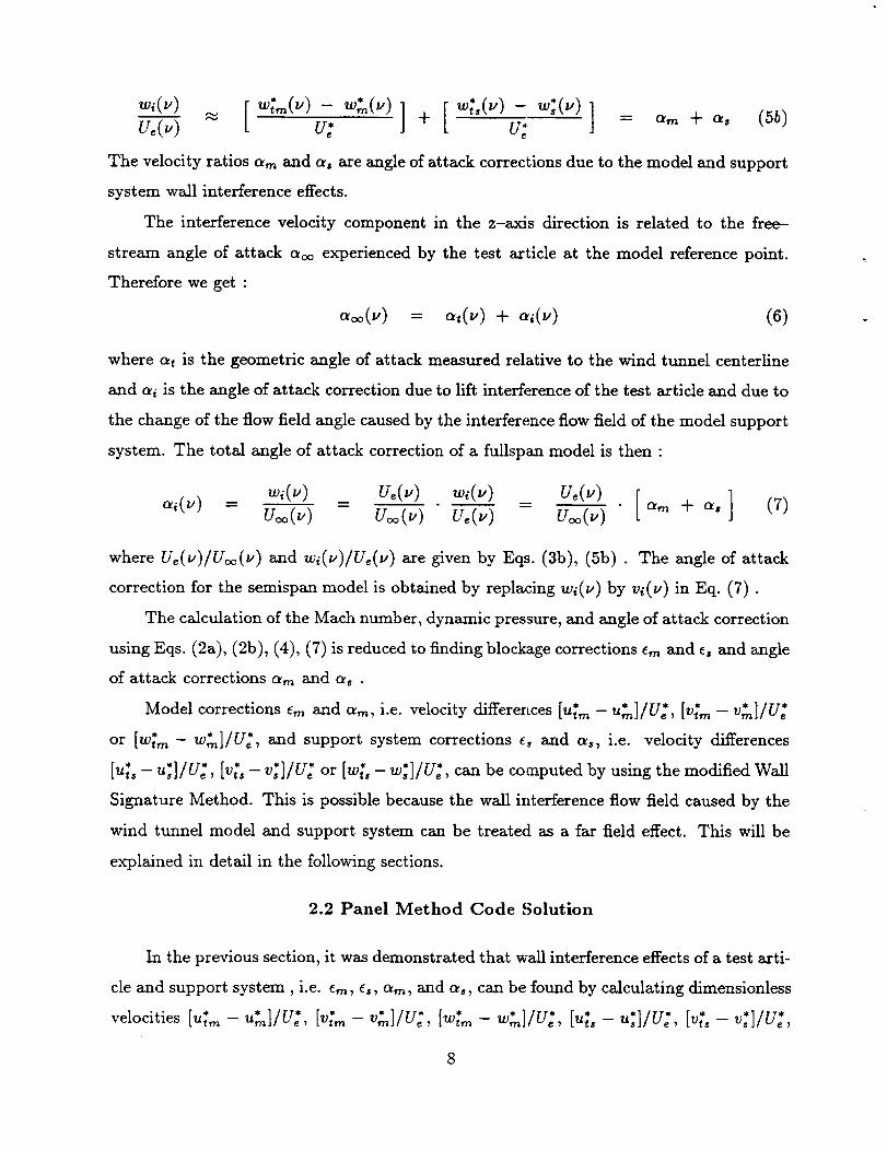
Wi(V) [ W _m (12 ) 1 r 1j + - j = +u,(.) L u: u;
The velocity ratios a,,_ and a, are angle of attack corrections due to the model and support
system wall interference effects.
The interference velocity component in the z-axis direction is related to the free-
stream angle of attack aoo experienced by the test article at the model reference point.
Therefore we get :
aoo(_) = a,(_) + _(.) (6)
where a_ is the geometric angle of attack measured relative to the wind tunnel centerline
and _i is the angle of attack correction due to lift interference of the test article and due to
the change of the flow field angle caused by the interference flow field of the model support
system. The total angle of attack correction of a fullspan model is then :
_(_) = w_(_) = v_(_) w_(_) -_- u_(_) [ ]+ (7)uoo( ,) L
whereU_(_)/U_(_)and_,(_)/U_(_)aregivenbyEqs.(3b),(Sb).Theangleofattack
correction for the semispan model is obtained by replacing w_(v) by v_(v) in Eq. (7).
The calculation of the Mach number, dynamic pressure, and angle of attack correction
using Eqs. (2a), (2b), (4), (7) is reduced to finding blockage corrections c,_ and e, and angle
of attack corrections am and a_ .
Model corrections c,_ and am, i.e. velocity differences Jut*m - u,.n]/Ve, [v_m - v,_]/Ve
or [wt*m - w_n]/U* , and support system corrections es and as, i.e. velocity differences
[u;, - u_]/U_, [v_, - v;]/U_ or [w;, - w_]/U*, can be computed by using the modified Wall
Signature Method. This is possible because the wall interference flow field caused by the
wind tunnel model and support system can be treated as a far field effect. This will be
explained in detail in the following sections.
2.2 Panel Method Code Solution
In the previous section, it was demonstrated that wall interference effects of a test arti-
cle and support system, i.e. e,_, e,, a,_, and as, can be found by calculating dimensionless
velocities [u_,_ - u*]/U*, [v_,_ - v_,]/U_, [w_ - w*]/U_, [u;_ - u*_]/U_, [v_s - v*]/U*,
and [w;, - w*]/U_ at a selected test article reference point v. These dimensionless veloc-
ities are computed by superimposing panel method code solutions and applying the Wall
Signature Method. In real-time operation, the Wall Signature Method uses a singularity
representation of the test article in combination with the measurement of wall pressure, lift
force, propulsion simulator thrust force, pitching moment, mad precalculated normalized
perturbation velocities to predict model wall interference corrections. The Wall Signature
Method may also be used to predict support system wall interference corrections by taking
the difference between the wall pressure port calibration of the support system and empty
tunnel. However, the application of the Wall Signature Method is only possible, if precal-
culated solutions of the subsonic potential equation in the form of normalized perturbation
velocities are linear with respect to singularity strength.
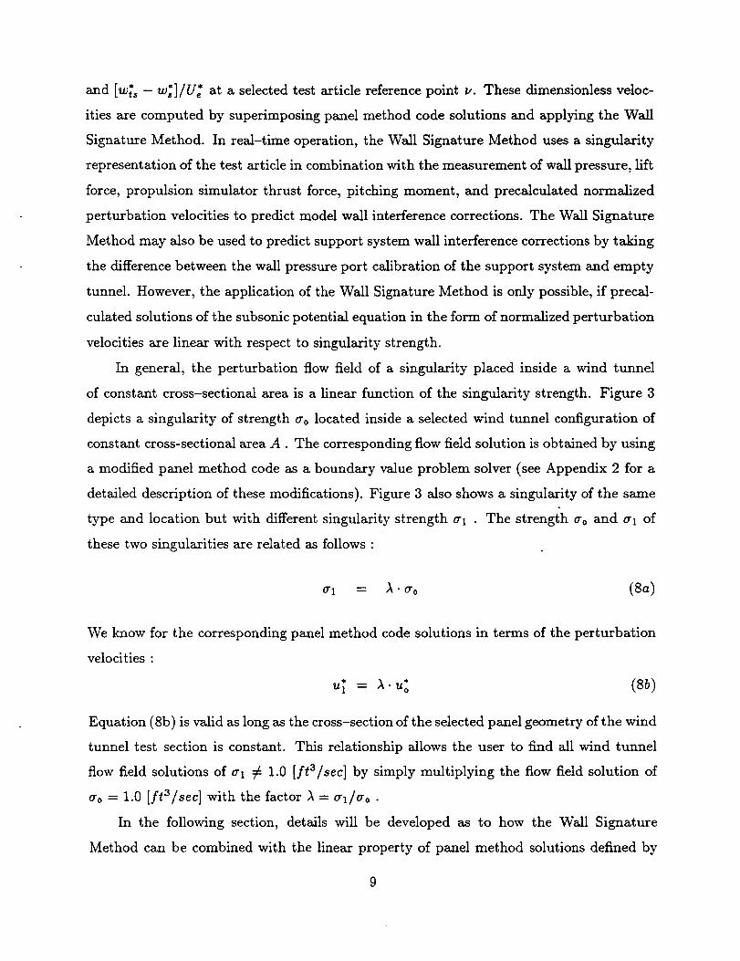
In general, the perturbation flow field of a singularity placed inside a wind tunnel
of constant cross-sectional area is a linear function of the singularity strength. Figure 3
depicts a singularity of strength _o located inside a selected wind tunnel configuration of
constant cross-sectional area A. The corresponding flow field solution is obtained by using
a modified panel method code as a boundary value problem solver (see Appendix 2 for a
detailed description of these modifications). Figure 3 also shows a singularity of the same
type and location but with different singularity strength _rl . The strength g0 and al of
these two singularities are related as follows :
or1 -- _.cr0 (8a)
We know for the corresponding panel method code solutions in terms of the perturbation
velocities :
* = _ * (8b)It 1 • U o
Equation (Sb) is valid as long as the cross-section of the selected panel geometry of the wind
tunnel test section is constant. This relationship allows the user to find all wind tunnel
flow field solutions of or1 # 1.0 [ft3/sec] by simply multiplying the flow field solution of
a0 = 1.0 [ft31sec] with the factor A = allao •
In the following section, details will be developed as to how the Wall Signature
Method can be combined with the linear property of panel method solutions defined by
9
Eqs. (Sa),(Sb) to obtain test article and support systemwall interferencecorrectionsfor a
a fullspan or semispan model.
2.3 Fullspan Model
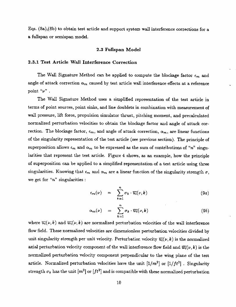
2.3.1 Test Article Wall Interference Correction
The Wall Signature Method can be applied to compute the blockage factor e_n and
angle of attack correction _,n caused by test article wall interference effects at a reference
point "v"
The Wall Signature Method uses a simplified representation of the test article in
terms of point sources, point sinks, and line doublets in combination with measurement of
wall pressure, lift force, propulsion simulator thrust, pitching moment, and precalculated
normalized perturbation velocities to obtain the blockage factor and angle of attack cor-
rection. The blockage factor, era, and angle of attack correction, am, are linear functions
of the singularity representation of the test article (see previous section). The principle of
superposition allows em and am to be expressed as the sum of contributions of "n" singu-
larities that represent the test article. Figure 4 shows, as an example, how the principle
of superposition can be applied to a simplified representation of a test article using three
singularities. Knowing that e,_ and a,_ are a linear function of the singularity strength _,
we get for "n" singularities :
?'4
= (ga)k--1
= (gb)k=l
where _¥(v, k) and _7(v, k) are normalized perturbation velocities of the wall interference
flow field. These normalized velocities are dimensionles_ perturbation velocities divided by
unit singularity strength per unit velocity. Perturbation velocity _-(v, k) is the normalized
axial perturbation velocity component of the wall inte_erence flow field and _'_(v, k) is the
normalized perturbation velocity component perpendicular to the wing plane of the test
article. Normalized perturbation velocities have the unit [1/rn 2] or [1/ft 2] . Singularity
strength _k has the unit [m 2] or [ft 2] and is compatible with these normalized perturbation
10
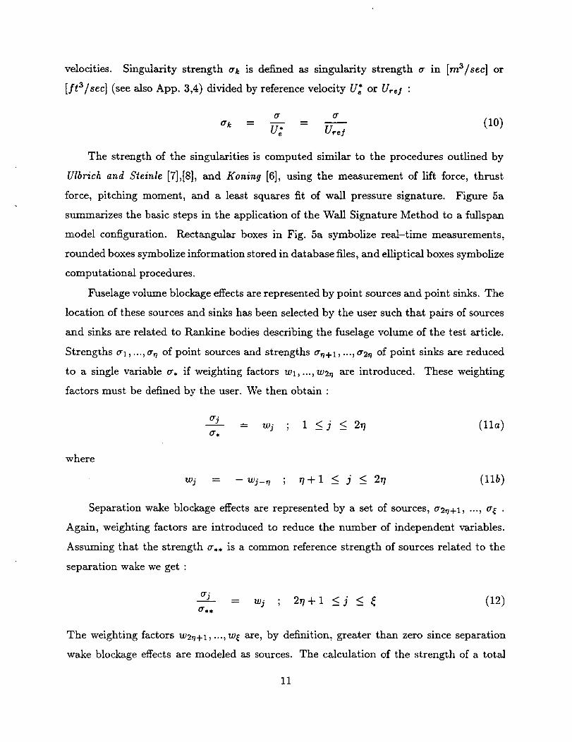
velocities. Singularity strength 0-k is defined as singularity strength 0- in [rn3/sec] or
[fta/sec] (see also App. 3,4) divided by reference velocity U* or U_, I :
0- O"
0-k = = (10)u;' u,- s
The strength of the singularities is computed similar to the procedures outlined by
Vlbrich and S_eiule [7],[8], and Kouing [6], using the measurement of lift force, thrust
force, pitching moment, and a least squares fit of wall pressure signature. Figure 5a
summarizes the basic steps in the application of the Wall Signature Method to a fullspan
model configuration. Rectangular boxes in Fig. 5a symbolize real-time measurements,
rounded boxes symbolize information stored in database files, and elliptical boxes symbolize
computational procedures.
Fuselage volume blockage effects are represented by point sources and point sinks. The
location of these sources and sinks has been selected by the user such that pairs of sources
and sinks are related to Rankine bodies describing the fuselage volume of the test article.
Strengths trl,..., 0-*?of point sources and strengths 0-*?+1, ..., 0-2*?of point sinks are reduced
to a single variable or. if weighting factors wl, ..., w2*? are introduced. These weighting
factors must be defined by the user. We then obtain :
_j= wj ; 1 <j < 21/ (lla)
0-,
where
wj = -wj_*? ; 7/+1 _< j _< 27/ (llb)
Separation wake blockage effects are represented by a set of sources, o"2,?+1, ..., 0-_¢ .
Again, weighting factors are introduced to reduce the number of independent variables.
Assuming that the strength a** is a common reference strength of sources related to the
separation wake we get :
= wj ; 2r/+l <j < _ (12)0-**
The weighting factors w2*?+l,..., w_ are, by definition, greater than zero since separation
wake blockage effects are modeled as sources. The calculation of the strength of a total
11
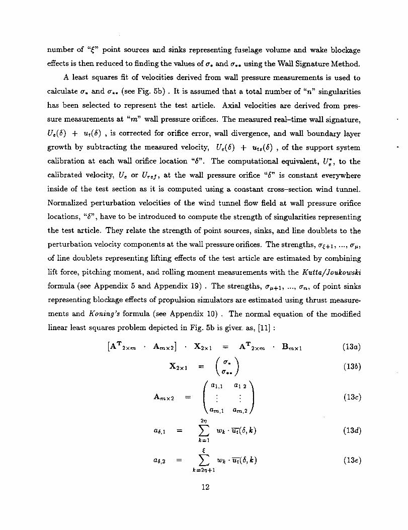
number of "_" point sources and sinks representing fuselage volume and wake blockage
effects is then reduced to finding the values of a, and a** using the Wall Signature Method.
A least squares fit of velocities derived from wall pressure measurements is used to
calculate a, and or,, (see Fig. 5b) . It is assumed that a total number of "n" singularities
has been selected to represent the test article. Axial velocities are derived from pres-
sure measurements at "m" wall pressure orifices. The measured real-time wall signature,
U_(_) + ut(6) , is corrected for orifice error, wall divergence, and wall boundary layer
growth by subtracting the measured velocity, Ue(d_) -_- uts(_) , of the support system
calibration at each wall orifice location "_". The computational equivalent, U_, to the
calibrated velocity, U_ or Ur_f, at the wall pressure orifice "6" is constant everywhere
inside of the test section as it is computed using a constant cross-section wind tunnel.
Normalized perturbation velocities of the wind tunnel flow field at wall pressure orifice
locations, "_", have to be introduced to compute the strength of singularities representing
the test article. They relate the strength of point sources, sinks, and line doublets to the
perturbation velocity components at the wall pressure orifices. The strengths, _+1, ..., _r_,
of line doublets representing lifting effects of the test article are estimated by combining
lift force, pitching moment, and rolling moment measuxements with the Kutia/Joukowski
formula (see Appendix 5 and Appendix 19) . The strengths, _,+1, ..., _r,_, of point sinks
representing blockage effects of propulsion simulators axe estimated using thrust measure-
ments and Koning's formula (see Appendix 10) . The normal equation of the modified
linear least squares problem depicted in Fig. 5b is giver., as, [11] :
[AT2 xrn Amx2] X2xl = AT2×,_ B,_×I (13a)
X2xl -" O'**
al,1 al 2 )Arnx2 "- " " (13c)
\ arn,1 am,2
2t7
a6,1 =
k=l
a6,2 :-
w,(6,k) (13 )
wk. _'7(,5, k) (13e)k=2,_+l
12
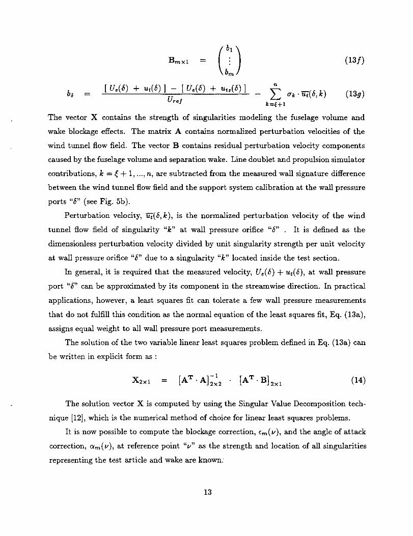
(b,). (13D
b_ = [U,(6) -+ u,(6)] - [Ue(6) + uts(6)] _ -h-7(6,k) (139)- z._.,o'kU,- S
k=_+1
The vector X contains the strength of singularities modeling the fuselage volume and
wake blockage effects. The matrix A contains normalized perturbation velocities of the
wind tunnel flow field. The vector B contains residual perturbation velocity components
caused by the fuselage volume and separation wake. Line doublet and propulsion simulator
contributions, k = _ + 1, ..., n, are subtracted from the measured wall signature difference
between the wind tunnel flow field and the support system calibration at the wall pressure
ports "6" (see Fig. 5b).
Perturbation velocity, _(6, k), is the normalized perturbation velocity of the wind
tunnel flow field of singularity "k" at wall pressure orifice "6" It is defined as the
dimensionless perturbation velocity divided by unit singularity strength per unit velocity
at wall pressure orifice "£' due to a singularity "k" located inside the test section.
In general, it is required that the measured velocity, U_(6) + ut(6), at wall pressure
port "6" can be approximated by its component in the streamwise direction. In practical
applications, however, a least squares fit can tolerate a few wall pressure measurements
that do not fulfill this condition as the normal equation of the least squares fit, Eq. (13a),
assigns equal weight to all wall pressure port measurements.
The solution of the two variable linear least squares problem defined in Eq. (13a) can
be written in explicit form as :
= [A A]-'2×2 [AT " B]2×l
The solution vector X is computed by using the Singular Value Decomposition tech-
nique [12], which is the numerical method of choice for linear least squares problems.
It is now possible to compute the blockage correction, c,_(v), and the angle of attack
correction, c_,_(v), at reference point "v" as the strength and location of all singularities
representing the test article and wake are known:
13
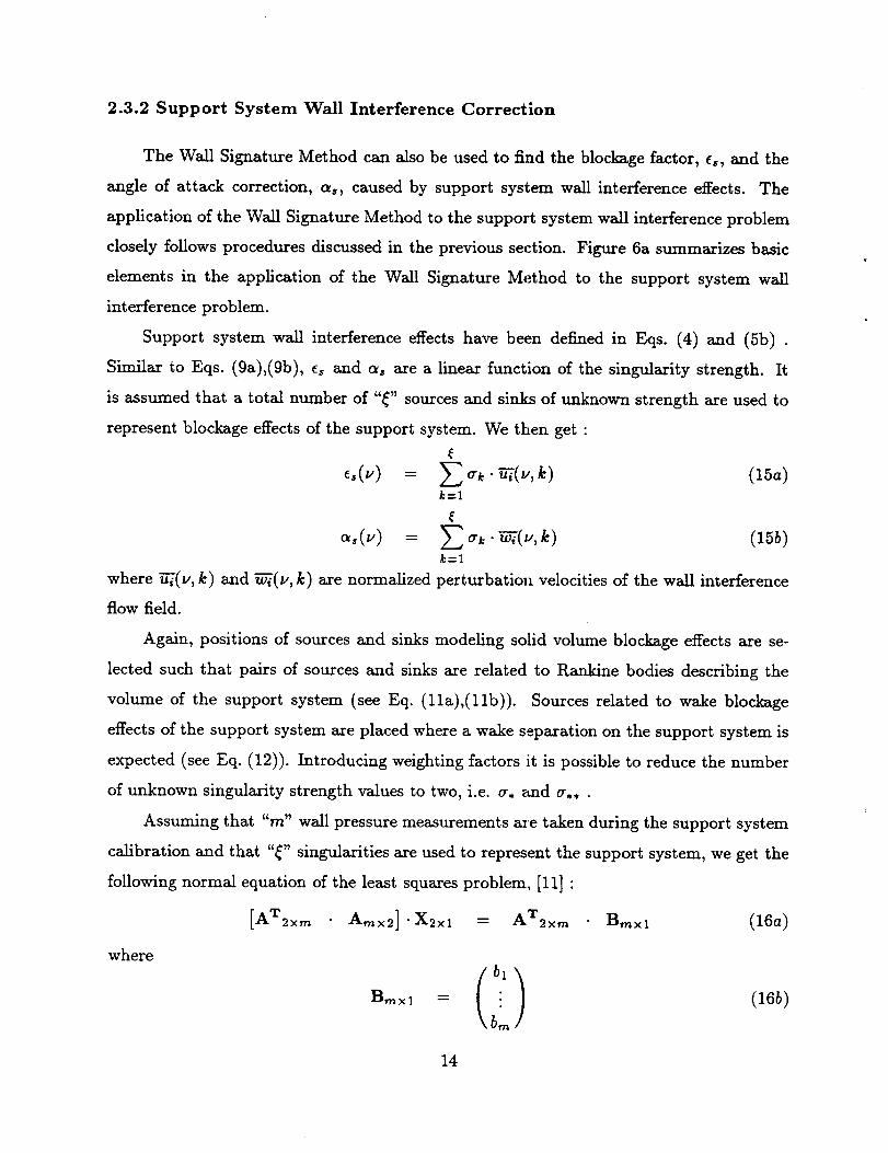
2.3.2 Support System Wall Interference Correction
The Wall Signature Method can also be used to find the blockage factor, es, and the
angle of attack correction, as, caused by support system wall interference effects. The
application of the Wall Signature Method to the support system wall interference problem
closely follows procedures discussed in the previous section. Figure 6a summarizes basic
elements in the application of the Wall Signature Method to the support system wall
interference problem.
Support system wall interference effects have been defined in Eqs. (4) and (5b) .
Similar to Eqs. (9a),(9b), e_ and as are a linear function of the singularity strength. It
is assumed that a total number of "_" sources and sinks of unknown strength are used to
represent blockage effects of the support system. We then get :
= (15a)k=l
k=l
where _'7(v, k) and _'(_,, k) are normalized perturbation velocities of the wall interference
flow field.
Again, positions of sources and sinks modeling solid volume blockage effects are se-
lected such that pairs of sources and sinks are related to Rankine bodies describing the
volume of the support system (see Eq. (lla),(llb)). Sources related to wake blockage
effects of the support system are placed where a wake separation on the support system is
expected (see Eq. (12)). Introducing weighting factors it is possible to reduce the number
of unknown singularity strength values to two, i.e.a. _md a** .
Assuming that "m" wall pressure measurements a_e taken during the support system
calibration and that "_" singularities are used to represent the support system, we get the
following normal equation of the least squares problem, [11] :
[AT ×m Am×s] = (16 )
wherebl
14
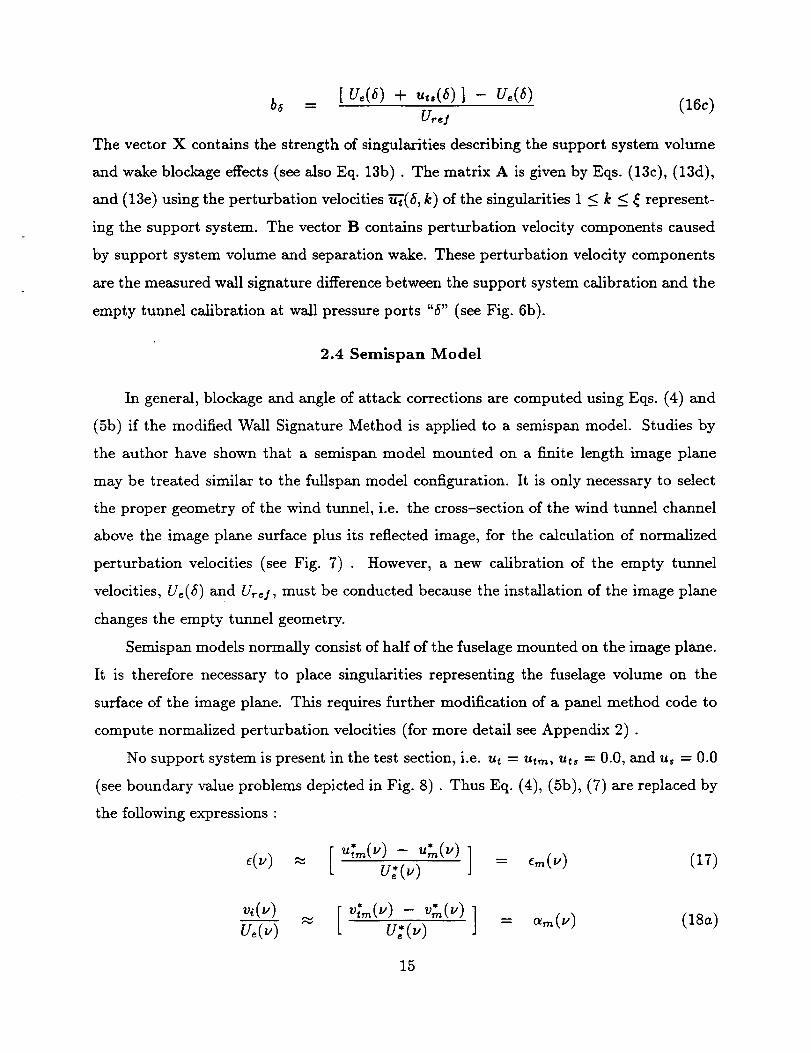
b6 = [U,(6) + u,,(_)] - U,(6) (16c)U,._.f
The vector X contains the strength of singularities describing the support system volume
and wake blockage effects (see also Eq. 135). The matrix A is given by Eqs. (13c), (13d),
and (13e) using the perturbation velocities _-t(6, k) of the singularities 1 < k _ _ represent-
ing the support system. The vector B contains perturbation velocity components caused
by support system volume and separation wake. These perturbation velocity components
are the measured wall signature difference between the support system calibration and the
empty tunnel calibration at wall pressure ports "_" (see Fig. 6b).
2.4 Semispan Model
In general, blockage and angle of attack corrections are computed using Eqs. (4) and
(5b) if the modified Wall Signature Method is applied to a semispan model. Studies by
the author have shown that a semispan model mounted on a finite length image plane
may be treated similar to the fullspan model configuration. It is only necessary to select
the proper geometry of the wind tunnel, i.e. the cross-section of the wind tunnel channel
above the image plane surface plus its reflected image, for the calculation of normalized
perturbation velocities (see Fig. 7) . However, a new calibration of the empty tunnel
velocities, U,(_) and U,.,I, must be conducted because the installation of the image plane
changes the empty tunnel geometry.
Semispan models normally consist of half of the fuselage mounted on the image plane.
It is therefore necessary to place singularities representing the fuselage volume on the
surface of the image plane. This requires further modification of a panel method code to
compute normalized perturbation velocities (for more detail see Appendix 2) .
No support system is present in the test section, i.e. ut = utm, uts = 0.0, and us = 0.0
(see boundary value problems depicted in Fig. 8). Thus Eq. (4), (55), (7) are replaced by
the following expressions :
- = (17)
~ = (18 )
15
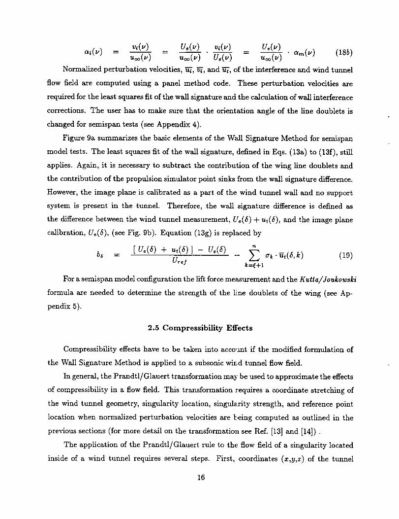
=
Normalized perturbation velocities, ui, vi, and _-t, of the interference and wind tunnel
flow field are computed using a panel method code. These perturbation velocities are
required for the least squares fit of the wall signature and the calculation of wall interference
corrections. The user has to make sure that the orientation angle of the line doublets is
changed for semispan tests (see Appendix 4).
Figure 9a summarizes the basic elements of the Wall Signature Method for semispan
model tests. The least squares fit of the wall signature, defined in Eqs. (13a) to (13f), still
applies. Again, it is necessary to subtract the contribution of the wing line doublets and
the contribution of the propulsion simulator point sinks from the wall signature difference.
However, the image plane is calibrated as a part of the wind tunnel wall and no support
system is present in the tunnel. Therefore, the wall signature difference is defined as
the difference between the wind tunnel measurement, Lr(6) + u_(6), and the image plane
calibration, U_(6), (see Fig. 95). Equation (13g) is replaced by
urns - (19)k=_+l
For a semispan model configuration the lift force measurement and the Kutta/Joukowski
formula are needed to determine the strength of the line doublets of the wing (see Ap-
pendix 5).
2.5 Compressibility Effects
Compressibility effects have to be taken into account if the modified formulation of
the Wall Signature Method is applied to a subsonic wind tunnel flow field.
In general, the Prandtl/Glauert transformation may be used to approximate the effects
of compressibility in a flow field. This transformation requires a coordinate stretching of
the wind tunnel geometry, singularity location, singulexity strength, and reference point
location when normalized perturbation velocities are being computed as outlined in the
previous sections (for more detail on the transformation see Ref. [13] and [14]).
The application of the Prandtl/Glauert rule to the flow field of a singularity located
inside of a wind tunnel requires several steps. First, coordinates (x,y,z) of the tunnel
16
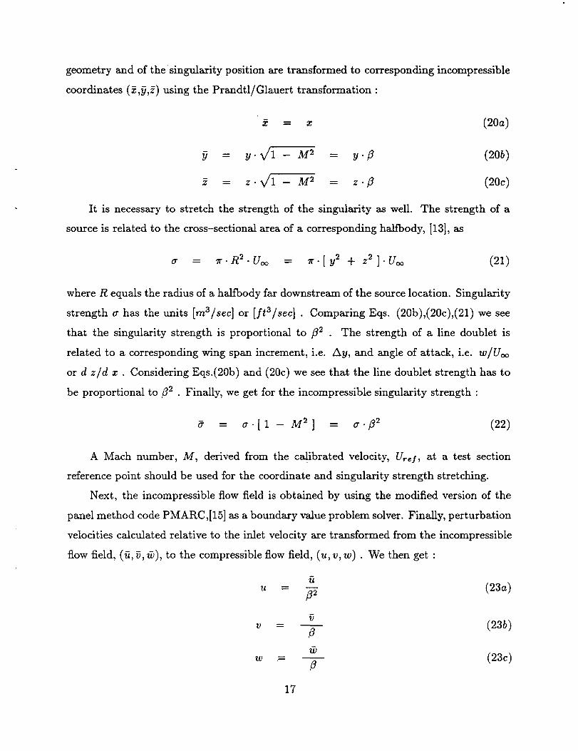
geometry and of the singulaz-ity position are transformed to corresponding incompressible
coordinates (_,_,_) using the Prandtl/Glauert transformation:
= • (20a)
= y.v/1 - M 2 - y-;3
5" = z.X/1 - M 2 = z.fl
It is necessary to stretch the strength of the singularity as well.
(20b)
(20c)
The strength of a
source is related to the cross-sectional area of a corresponding halfbody, [13], as
= .R2.Uoo = + z2].Uoo (21)
where R equals the radius of a halfbody far downstream of the source location. Singularity
strength cr has the units [m3/sec] or [ft3/sec]. Comparing Eqs. (20b),(20c),(21) we see
that the singularity strength is proportional to f12 . The strength of a line doublet is
related to a corresponding wing span increment, i.e. Ay, and angle of attack, i.e. w/Uoo
or d z/d z. Considering Eqs.(20b) and (20c) we see that the line doublet strength has to
be proportional to f12 . Finally, we get for the incompressible singularity strength :
= a.[1 - M 21 = cr.t32 (22)
A Mach number, M, derived from the calibrated velocity, U_el , at a test section
reference point should be used for the coordinate and singularity strength stretching.
Next, the incompressible flow field is obtained by using the modified version of the
panel method code PMARC,[15] as a boundary value problem solver. Finally, perturbation
velocities calculated relative to the inlet velocity are transformed from the incompressible
flow field, (fi, _, _), to the compressible flow field, (u, v, w). We then get :
fi
u = _-_ (23a)
W "-"
fl (23b)
fl (23c)
17
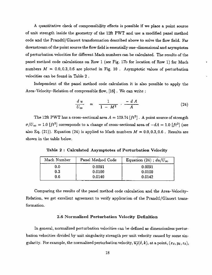
A quantitative checkof compressibility effects is possible if we place a point source
of unit strength inside the geometry of the 12ft PWT and use a modified panel method
code and the Prandtl/Glauert transformation described above to solve the flow field. Far
downstream of the point source the flow field is essentially one-dimensional and asymptotes
of perturbation velocities for different Mach numbers can be calculated. The results of the
panel method code calculations on Row 1 (see Fig. 17b for location of Row 1) for Mach
numbers M - 0.0, 0.3, 0.6 are plotted in Fig. 10 . Asymptotic values of perturbation
velocities can be found in Table 2 .
Independent of the panel method code calculation it is also possible to apply the
Area-Velocity-Relation of compressible flow, [16] . We can write :
du 1 -dA
Uoo = 1- M 2 A (24)
The 12ft PWT has a cross-sectional area A = 109.74 [ft 2] . A point source of strength
a/Uoo = 1.0 [ft 2] corresponds to a change of cross-sectional area of -dA = 1.0 [ft 2] (see
also Eq. (21)). Equation (24) is applied to Mach numbers M - 0.0, 0.3, 0.6. Results are
shown in the table below.
Table 2 : Calculated Asymptotes of Perturbation Velocity
Mach Number Panel Method Code Equation (24) ; du/Uoo
0.0 0.0091 0.0091
0.3 0.0100 0.0100
0.6 0.0140 0.0142
Comparing the results of the panel method code calculation and the Area-Velocity-
Relation, we get excellent agreement to verify application of the Prandtl/Glauert trans-
formation.
2.6 Normalized Perturbation Velocity Definition
In general, normalized perturbation velocities can be defined as dimensionless pertur-
bation velocities divided by unit singularity strength per unit velocity caused by some sin-
gularity. For example, the normalized perturbation velocity, _-/(_, k), at a point, (x_, y$, z6),
18
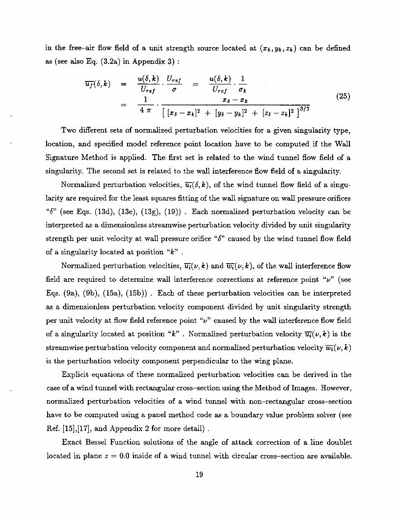
in the free-air flow field of a unit strength source located at (zk, Yk, z_) can be defined
as (seealsoEq.(3.2a)in Appenaix3):
_(6, k) = u(6,k) Vro: = _(_,k___2).iU,._: o" U,._I o'21 x_- zk (25)
4 _ [ [x, - _]2 + [_ _ _]2 + [z_- z_]_]3/2
Two different sets of normalized perturbation velocities for a given singularity type,
location, and specified model reference point location have to be computed if the Wall
Signature Method is applied. The first set is related to the wind tunnel flow field of a
singularity. The second set is related to the wall interference flow field of a singularity.
Normalized perturbation velocities, h-7(6, k), of the wind tunnel flow field of a singu-
larity are required for the least squares fitting of the wall signature on wall pressure orifices
"5" (see Eqs. (13d), (13e), (13g), (19)) . Each normalized perturbation velocity can be
interpreted as a dimensionless streamwise perturbation velocity divided by unit singularity
strength per unit velocity at wall pressure orifice "6" caused by the wind tunnel flow field
of a singularity located at position "k"
Normalized perturbation velocities, _-(v, k) and _'(v, k), of the wall interference flow
field are required to determine wall interference corrections at reference point "v" (see
Eqs. (9a), (95), (15a), (155)) . Each of these perturbation velocities can be interpreted
as a dimensionless perturbation velocity component divided by unit singularity strength
per unit velocity at flow field reference point "L," caused by the wall interference flow field
of a singularity located at position "k" . Normalized perturbation velocity _--_(v, k) is the
streamwise perturbation velocity component and normalized perturbation velocity _-(v, k)
is the perturbation velocity component perpendicular to the wing plane.
Explicit equations of these normalized perturbation velocities can be derived in the
case of a wind tunnel with rectangular cross-section using the Method of Images. However,
normalized perturbation velocities of a wind tunnel with non-rectangular cross-section
have to be computed using a panel method code as a boundary value problem solver (see
aef. [15],[17], mad Appendix 2 for more detail).
Exact Bessel Function solutions of the angle of attack correction of a line doublet
located in plane z = 0.0 inside of a wind tunnel with circular cross-section are available.
19

NACA TN 2454, [18] lists these corrections in the form of upwash factor tables. Tables
can be compared with the normalized perturbation velocities of the wall interference flow
field that were computed using a modified panel method code [15],[17].
At first, an upwash factor table used for fullspan model tests (Table I on p.32 of NACA
TN 2454, [18]) is compared with the corresponding panel method code solution. Figs. lla
and 1 lb compare upwash factor F as a function of the dimensionless streamwise coordinate
and the dimensionless line doublet location (lateral coordinate !? = 0.7). The exact Bessel
Function solution and the numerical panel method code solution of the upwash factor F
show reasonable agreement verifying the normalized perturbation velocity definition of the
fullspan configuration.
Table 3 compares the input and accuracy characteristics of NACA TN 2454 and the
panel method code solution of the normalized perturbation velocities.
Table 3 : Comparison NACA TN 2454 / Panel Method Code
NACA TN 2454 Panel Method Code
Tunnel Circular Tunnel Any Tunnel Geometry
Geometry One Bipolar Tunnel
Solution
Type
Exact (Circular)
Approximation (Bipolar)
Singularity Line Doublet
Type
Singularity Z=0.0 (Circular)
Location Y=0.0 (Bipolar)
Reference Point Z=0.0 (Circular)
Location Y=0.0 (Bipolar)
Numerical
Solution
Point Source, Point Doublet,Line Doublet
Minimum distance from wall
panels _ 0.2 × tunnel radius
Minimum distance from wall
panels .._ 0.2 × tunnel radius
Unfortunately, no rigorous solution of the upwash factor F, i.e. angle of attack cor-
rection, of a line doublet located inside of a bipolar wind tunnel (image plane / semispan
configuration) is available. However, NACA TN 2454 provides an approximation of the
upwash factor F for a bipolar wind tunnel that can be compared with the results obtained
by applying a panel method code. Fig. 11c compares tl:.is approximation of upwash factor
F (Fig. 5(c) on p.56 of NACA TN 2454, [18]) with the panel method code solution. Both
approximations show reasonable agreement verifying the normalized perturbation velocity
2O
definition of the semispanmodel configuration.
A panelmethod codeallows the userto computenormalizedperturbation velocities for
any type of constant cross-sectionwind tunnel geometrythat canbe paneled. Singularities
and referencepoints can alsobe placed anywhereinside of the wind tunnel as long asthe
minimum distanceof the singularity or referencepoint from the paneledwind tunnel wall
(60 panelsused to representtunnel cross-section)is greater than 0.2 x tunnel radius.
21
22
CHAPTER3
APPLICATION OF THE METHOD TO WIND TUNNEL TESTS
3.1 Real-Time Wall Interference Calculation
The revised and improved version of the Wall Signature Method presented in this
report can be used to predict the Mach number, dynamic pressure, and angle of attack
correction at a test article reference point due to the subsonic wind tunnel wall interference
effects. Post-test analysis of subsonic wall interference effects is also possible as long as
the exact position of the test article in the wind tunnel is known for a specific angle of
attack setting. The location of singularities representing the test article is directly related
to this position. Perturbation velocities of the wind tunnel and interference flow field can
be computed as outlined in the previous chapters.
The real-time calculation of wall interference corrections is fast because the Wall
Signature Method only requires superposition of the perturbation velocities, application
of the Kutla/Jonkowski formula (Appendix 5), Koning's formula (Appendix 10), and the
solution of a 2 x 2 linear system of equations related to the least squares fit of the wall
signature.
The precalculation of normalized perturbation velocities used for the real-time least
squares fit of the wall signatures and for the calculation of corrections has to be done on a
mainfraxne computer or fast workstation since a realistic implementation of the proposed
Wall Signature Method requires the calculation of perturbation velocities for many different
singularity types, locations, and Math numbers. Figures 12a,12b depict geometries of the
NASA 12ft Pressure Wind Tunnel test section that are selected for the calculation of the
perturbation velocities of the wind tunnel and interference flow field using a panel method
code as a boundary value problem solver. Preeomputed normalized perturbation velocities
have to be stored in a database that is accessed during a wind tunnel test.
A singularity and reference point grid has to be used for the calculation of the per-
turbation velocity database. These two grids should be selected such that they allow for
a real-time interpolation of all conceivable singularity and reference point locations in the
wind tunnel test section. Perturbation velocities required for singularities representing the
23
test article changeas a function of test article geomel;ry and position in the wind tun-
nel test section. Size, complexity, and accuracy requirements of the perturbation velocity
database have to be balanced to guarantee best real-time performance. Thus, perturbation
velocities of the wind tunnel and interference flow field for a given test article location are
found in real-time by applying a tri-linear interpolation (real-time singularity position;
Appendix 6) and parabolic interpolation (real-time Mach number; Appendix 7) to the
precomputed perturbation velocity database.
Blockage effects of the support system can be computed off-line by applying the Wall
Signature Method to the difference between the support system and the empty tunnel
calibration. Computed support system wall interference corrections on the reference point
grid have to be stored in a database as a function of the support system calibration
variables. The support system wall interference corrections are added in real-time to the
wall interference corrections caused by the test article.
Post-test analysis of the interference effects is based on minimizing the standard
deviation of the least squares fit of the wall signature as a function of the location of the
test article singularities (see Appendix 8). This procedure provides an optimal singularity
representation of the test article.
Studies of the author have shown that the real-t:ime speed of the wall interference
calculation is governed by the efficiency of the interpolation of the perturbation velocities
using the precomputed perturbation velocity database.
Figures 13a,13b depict basic elements of the real-time Wall Signature Method for
a fullspan and a semispan model configuration. The .empty tunnel calibration, support
system calibration, real-time wall pressures , lift force, propulsion simulator thrust, and
pitching moment measurements are the critical link between experiment and the panel
method code calculation. Matching conditions between the wind tunnel test and the panel
method code calculation will be discussed in detail in the following section.
3.2 Matching Conditions
The least squares fit proposed for a fullspan and semispan model configuration relates
experimental data, i.e. wall pressure measurements, to precomputed normalized perturba-
24
tion velocities. Therefore suitable equationshave to be found to convert the wall pressure
measurementsto perturbation velocities.
Perturbation velocity differences [U, + ut] - [U, + ut,] , [U, + ut,] - U, , and [U, + ut] -
U, defined in Eqs. (13g), (16c), and (19) can be related to the wall pressure measurements
taken during calibration and real-time wind tunnel test by applying the energy equation
and the isentropic flow assumption. Assuming that the total temperature TT and total
pressure PT in the tunnel settling chamber, and the static pressure p at wall pressure orifice
are known, we get for the flow velocity (see Fig. 14a) :
Dimensionless perturbation velocities can then be written as :
[U_(6) + ut(6)]- [ U_(cS) + ut,(_5)] = V(pt,,,_(tS))- U(p_,_v(_5)) (27a)U,._ I U_<f
[ + - u0(6) - u(v mp(6))= (27b)
u_s u_f
[ uo(6) + - u (6) -= (27c)
U,._ I U,._S
The flow velocity U(p(6)) in Eq. (26) is written as a function of the pressure difference
PT -- P(_) as it is easier to measure a pressure difference at a wall pressure port. Real-time
static pressure pt_,,-,, support system static pressure ps=p, and empty tunnel calibration
static pressure Pemp are recorded at each wall pressure port "_" . Measured velocity
Ue(_) = U(pe,-r,p($)) at a wall pressure port "_" is the first matching condition. It is
required to obtain the perturbation velocities defined in Eqs. (27b),(27c).
The velocity Ur_f in Eqs. (13g), (16c), and (19) is the second matching condition
between the wind tunnel flow field and the corresponding dimensionless panel method
code calculation. It is required to non-dimensionalize the perturbation velocities defined
in Eqs. (27a),(27b),(27c) . It can be considered as the constant flow velocity inside of
a hypothetical constant cross-sectional test section. This velocity should be measured
during the empty tunnel calibration at a specific model reference point 0 (see Fig. 14b;
this point has the coordinates X=120.71 [ft], Y=0.0 [ft], Z=0.0 [ft] in the 12ft PWT). The
25
velocity Urel can be measured by using, e.g., a static pipe installed in the wind tunnel
during the calibration. We then get :
: [The real-time lift force _nd pitching moment measurements are related to the strength
of the corresponding line doublets using the Kn_ta/Joukowski formula. Its application re-
quires knowledge of velocity U,-ef and density p,..! (0) at a model reference point 0 measured
during the calibration of the wind tunnel. This velocity and fluid density connect lift force
and pitching moment measured in [lbf],[ft • lbf] or [NI,[N • m] to the definition of the
line doublet strength in [ft 2] or [m 2] (see Appendix 5). The fluid density is also required
to relate the propulsion simulator thrust measurement to the sink strength if Koniug's
formula is applied (see Appendix 10). The density P,-e! (9) is the third matching condition.
It is found by applying the ideal gas and the isentropic flow relationship at a test section
reference station/9 . We get :
e s(0) = R-- r " -- (29)
where p_mp(0) is the static pressure measured at the model reference point/9 .
It is interesting to note that the perturbation velocity differences [Ue(6) + ut(6)] -
[V_(6) + ut_(6)], [g_(6) + u,,(6)] - U_(d_), and [U_(6) + u,(6)] - U_(6) remove the influence
of the wall boundary layer growth, orifice error, image plane, and wall divergence from the
least squares fit. Therefore it is possible to use the geometry of an equivalent wind tunnel
with constant cross-sectional area for the calculation of normalized perturbation velocities
of the wind tunnel and interference flow field.
Three matching conditions, i.e. U_(6), U_S, and .o,-_I, establish a link between the
measurement of wall pressures, forces, moments and the panel code solutions of the wind
tunnel and interference flow field expressed as normali2ed perturbation velocities. Figure
14c summarizes the importance of these matching conditions.
3.3 Application of the Method to Semlspan Models
In the summer of 1996, two different sized semispem models were tested in the NASA
Ames 12ft Pressure Wind Tunnel (PWT). Both models, i.e. the 8 % and 14 % scale 7J7
26
semispanmodels,were provided by the Boeing Corporation. Eachmodel wasmounted on
the image plane in the 12ft PWT. Figure 15showsa similar test configuration.
Both models were tested over a wide range of angle of attack, total pressure, and Mach
number settings. For the present study, two runs were selected. During Run No. 154 the
8 % scale model was tested from -20.280 to 19.820 uncorrected angle of attack at a total
pressure of 2.0 [atm] and a Mach number of 0.25 . During Run No. 219 the 14 % scale
model was tested from -4.030 to 9.980 uncorrected angle of attack at a total pressure of
2.0 [atm] and a Mach number of 0.30 .
The application of the present wall interference correction method was done in several
steps. At first, type and initial location of the singularities representing each model were
specified. Rules of thumb given in Appendix 9 were used to select type, location, and
weighting factors for these singularities. A total of 11 singularities were selected for each
model. A source and a sink were selected to represent fuselage blockage, two sources
were selected to model the separation wake blockage effects. Seven line doublets, located
along the 1/4 chord hne of the wing, were chosen to represent lifting effects. Weighting
factors for the line doublets were selected to model an elliptic lift distribution for the wing.
Figures 16a,16b give the singularity representation of each semispan model for 0 ° angle of
attack. The real-time coordinates of these singularities as a function of the pitch angle
were computed using the known kinematics of a semispan model mounted on the image
plane (for more detail see Eqs. (14.19a),(14.19b) in Appendix 14).
In the next step, measured lift force in combination with the Kulta-Joukowski formula
was used to determine the strength of line doublets for the wing for each data point.
The strength of the remaining singularities was computed using a least squares fit
of the wall pressure measurements on 180 wall pressure ports that were arranged in six
rows above the image plane. The least squares fit used wall pressure port rows 1,2,3,6,7,8
depicted in Fig. 17a,17b. For more detail on the least squares fit procedure see Section 2.4.
The standard deviation of the least squares fit of the wall signature was computed
for each data point of Runs 154 and 219 (see Figs. 18a,18b) . The standard deviation of
the 8 % scale model was on the order of 0.002 in units of the dimensionless perturbation
velocity. This agrees with the standard deviation of a wall signature obtained by Rueger et
al., [19] who reported a value of 0.005 in units of pressure coefficient, i.e. 0.0025 in units of
27
the dimensionlessperturbation velocity. The standard deviation of the 14 _ scalemodel
wason the order of 0.003 to 0.006in units of the dimensionlessperturbation velocity.
Figures 19ato 19f showthe result of the least squaresfit of the wall signature for the
8 % semispanmodel at 19.82o uncorrected angle of attack. Figures 20a to 20f show the
result of the least squares fit of the wall signature for the 14 % semispan model at 9.98 o
uncorrected angle of attack. Figures 21a, 21b depict the wall signature for both models at
approximately 0.0 ° angle of attack at wall pressure port Row 6 . The large difference in
solid volume blockage of both models can clearly be detected in the wall signature. The
measured wall signature difference "u" depicted in Figs. (19a) to (21b), i.e. the velocity
difference [Ue + ut] - Ue in Fig. 9b, shows excellent agreement with its least squares fit.
The present method (WICS), the two--variable method, and the classical method were
used to compute wall interference corrections. Two-variable method results were provided
by Mat Rueger of Boeing St. Louis. Classical corrections were provided by Alan Boone
of NASA ARC who used NACA Rep. No. 995 (solid volume blockage), [20], R.A.E. Rep.
No. 3400, [21] (separation wake blockage), and NACA TN 2454, [18], to determine wall
interference corrections. Mean wall interference corrections for each model were computed
using flow field reference points located along the 3/4 chord line of the wing. Corresponding
results are compared below.
As expected, wall interference corrections computed by WICS and the two-variable
method show excellent agreement because both methods are based on potential flow theory
and boundary flow measurements. Angle of attack corrections agree well in all three cases
(see Figs. 22a,22b) . The solid volume blockage factor contribution depicted in Fig. 23a
agrees well for the 8 % scale model in all three cases. A comparison of the solid volume
blockage factor contribution of the 14 % scale model depicted in Fig. 23b shows larger
differences between classical corrections and WICS. This can be explained by the fact
that the calculation of the solid volume blockage using the classical method (NACA Rep.
No. 995) assumes that a wind tunnel of constant cro,;s-section extends to far upstream
and downstream of the semispan model. This assumption, however, cannot be justified
anymore in the case of the 14 % scale model as the fllselage length is 16.69 [ft] and the
length of the image plane is _ 20.0 [ft] . The classica] method will therefore overpredict
the solid volume blockage effect for the 14 % scale model. The separation wake blockage
28
factorcontribution for the 8 % scalemodel determined based on the classicalmethod [21]
islargerthan the blockage factor computed using WICS or the two-variable method (see
Figs. 23a). This agrees with observations reported in the literature,[5],[19].
The 8 % and 14 % scale model have identicalgeometry. Therefore itis possible to
compare the minimum of the blockage factor of both models by using a scale factor law
(formore detailsee Appendix 20). Results discussed in Appendix 20 demonstrate that
blockage correctionscomputed with the present method (WICS) satisfythis scale factor
law. Thus, wall pressure measurement accuracy and the solidvolume descriptionused by
the present method are sufficientlyaccurate for computing blockage effects.
In general, the ratio between measurements and unknowns of a leastsquares fithas
to be large to take fulladvantage of its smoothing characteristics.In our application
the number of unknowns of the least squares fitis two (see Eqs. (13a),(16a)). Figures
23c, 23d compare the computed dynamic pressure correction for the 8 % scale model
with 180 or 30 wall pressure ports used for the least squares fit of the wall signature.
The differencesin the computed corrections depicted in Figs. 23c, 23d are small. This
demonstrates a key operational advantage of the Wall Signature Method : the calculation
of the correctionsisrelativelyinsensitiveto the number and location of the wall pressure
ports (see also Table 1 in Chapter 1) . Comparison of the data scatter in the computed
dynamic pressure correctiondepicted in Figs.23c,23d shows that an increase in the number
of wall pressure measurements used in the least squares fitreduces the data scatterof the
computed blockage corrections.
The local dynamic pressure correction for the 8 % model at 19.82° angle of attack
and for the 14 % model at 9.980 angle of attack are computed in the plane Y=0.0 [ft](cut
through test section parallelto side wall). The dynamic pressure correction for the 8 %
model at 19.82° increasesgradually as an observer moves from upstream to downstream
of the model (see Fig. 24a) . The separation wake blockage effectsdominate the dynamic
pressure correctiondownstream of the model at an angle of attack of 19.82° . The contour
linesare nearly parallelto the z-axis. We conclude that the dynamic pressure correction
for the 8 % model is almost exclusivelya function of the streamwise coordinate.
The dynamic pressure correctionfor the 14 % model at 9.98° has a saddle point at the
streamwise coordinate 120.0 [ft] (see Fig. 24b). The correction decreases as an observer
29
movesdownstream of the model. Therefore, it can be concluded that the solid volume
blockage effects dominate the correction at an angle of attack of 9.98 ° .
In both contour plots, it can be seen that the minimum of the dynamic pressure
correction for a constant streamwise coordinate is about 4.0 [ft] above the image plane.
This is caused by the fact that the tunnel width increases as an observer moves from the
image plane surface to the tunnel centerline (see also Fig. 15).
The local angle of attack corrections for 19.82 o and 9.98 o for each model are computed
in the plane Y=0.0 [ft] (cut through test section parallel to side wall). The contour plots
of the results are depicted in Figs. 24c,24d. The angle of attack correction variation along
the 3/4 chord line of the 8 % model at 19.82 °, i.e. from wing root to tip, is on the order
of 0.050 . The aerodynamic twist is insignificant in this case. However, the angle of attack
correction variation along the 3/4 chord line of the 14 % model at 9.98 ° is on the order of
1.0 ° and cannot be ignored anymore.
3.4 Application of the Method to the Ames Bipod
In 1995 the Ames Bipod, a floor-mounted support system, was tested in the NASA
Ames 12ft Pressure Wind Tunnel (PWT). Blockage corrections due to support system wall
interference effects were computed using the Wall Signature Method (WICS) as outlined
in Section 2.3.2 .
The application of the Wall Signature Method to t:ae Ames Bipod was done in several
steps. At first, type, initial location, and weight of singularities representing the Ames
Bipod were specified. Figure 25a shows the Ames Bipod geometry and lists type, initial
location, and weight of these singularities. A total number of 27 singularities was selected
for the support system. Singularities No. 1 to No. 18, i.e. 9 source/sink pairs, were chosen
to represent solid volume blockage effects of the support system. Singularities No. 19 to
No. 27 were chosen to model separation wake blockage effects.
In a second step, strength values of these singularities were computed using a least
squares fit of the wall pressure measurements. Wall pressures on Row 1 to Row 8 (see
Figs. 17a,17b) were measured during the support system calibration as a function of the
total pressure in the settling chamber and the Mach aumber at a test section reference
3O
point. Wall pressure measurements obtained during an empty tunnel calibration were also
available. The least squares fit was applied to the difference between the wall signature
measured during the support system calibration and the wall signature measured during
the empty tunnel calibration. Figures 25b,25c show the result of the least squares fit on
Row 2 and Row 4. Measured wall signature difference and least squares fit show reasonable
agreement. Larger differences between the measured wall signature and the least squares
fit on Row 4 are caused by the fact that singularities cannot be placed too close to the floor
for numerical reasons (see also Chapter 2.6). Finally, the blockage factor was computed on
planes Y=0.0 [ft] (parallel to test section side wall), X=120.71 [ft] (parallel to test section
inlet), and Z=0.0 [ft] (parallel to test section floor).
Figure 25d shows the blockage factor on plane Y=0.0 [ft] that was computed using
the initial singularity location given in Fig. 25a . Figure 25e shows the blockage factor
on plane Y=0.0 [ft] that was computed after the standard deviation of the least squares
fit was minimized as a function of the singularity location (see Appendix 8). Comparing
both contour plots it can be recognized that differences in the computed blockage factor
are small, i.e. computed corrections are not very sensitive to the location of singularities
as long as they are placed at the location of the support system. Comparing singularity
locations before and after the minimization it can be noticed that sources No. 1 to No. 9
and sources No. 19 to No. 27 have moved closer together. The minimization procedure
has correctly deduced from the wall signature difference that the front post of the Ames
Bipod has a significantly larger diameter than the pitch strut, i.e. most of the separtion
wake of the Ames Bipod is caused by the front post.
Figure 25f shows the blockage factor on plane X=120.71 [ft] . In this contour plot it
can be seen that the blockage factor increases in any direction if an observer moves closer
to the test section wall. A minimum of the blockage factor is located _ 1.0 [ft] above the
tunnel centerline. The blockage factor increases significantly if an observer moves closer
to the test section floor.
Figure 25g shows the blockage factor on plane Z=0.0 [ft] . As expected, the blockage
factor increases if an observer moves from an upstream position to a downstream position.
This observation is caused by the fact that the separtion wake blockage dominates blockage
corrections downstream of the Ames Bipod.
31
32
CHAPTER 4
CONCLUSION AND REMARKS
A revised version of the Wall Signature Method was developed which allows the user to
predict Math number, dynamic pressure, and angle of attack correction due to wall inter-
ference effects in three-dimensional subsonic wind tunnel testing of aircraft models. This
improved formulation of the Wall Signature Method uses lift force, propulsion simulator
thrust force, pitching moment, wall pressure measurements, empty tunnel calibration, sup-
port system calibration, a simplified representation of the test article and support system
in terms of singularities, and precalculated normalized solutions of the subsonic poten-
tial equation expressed as normalized perturbation velocities to predict wall interference
corrections at a model reference point in real-time.
The method is applicable to complex wind tunnel and support system configurations.
Wall interference corrections are found by taking the difference between a simplified rep-
resentation of the wind tunnel flow field in terms of singularities and the corresponding
free-air solution. Computational procedures were developed to predict solid body blockage,
separation wake blockage, propulsion simulator blockage, and lift interference correction if
a fullspan model or a semispan model is tested.
The definition of normalized perturbation velocities used by the method has been
improved to allow the user to take full advantage of the geometry modeling capabilities of
a three-dimensional panel method code. A "global" least squares fit procedure of the wall
signature was also introduced to improve the application of the Wall Signature Method
in real-time. Optimal locations of singularites are defined by minimizing the standard
deviation of the least squares fit of the wall signature.
Experimental data obtained during tests of two semispan models mounted on an image
plane in the NASA 12ft Pressure Wind Tunnel were applied to the modified Wall Signa-
ture Method. Blockage and angle of attack corrections were computed for different angle
of attack settings. In all cases, computed angle of attack corrections show good agree-
ment with corresponding classical corrections. Computed blockage corrections are smaller
than corresponding classical corrections. This result agrees with observations reported in
33
literature, [5],[19] .
Experimental data recorded during the calibration of the Ames Bipod was also suc-
cessfuUy applied to the method.
Further experimental studies have to be conducted in the future to gain confidence in
the method.
34
LIST OF REFERENCES
[1] Hackett, J. E., Wilsden, D. J. and Lilley, D. E., "Estimation of Tunnel Blockage
from Wall Pressure Signatures: a Review and Data Correlation," NASA CR-152241,
Lockheed-Georgia Company, Marietta, Georgia, March 1979.
[2] Hackett, J. E., Wilsden, D. J. and Stevens, W. A. , "A Review of the Wall Pressure
Signature and other Tunnel Constraint Correction Methods for High Angle-of-Attack
Tests," AGARD-R-692, Munich, May 1980.
[3] Hackett, J. E., "Living with Solid-Walled Wind Tunnels," AIAA 82-0583, presented at
the AIAA 12th Aerodynamic Testing Conference, March 22-24, 1982/Williamsburg,
Virginia.
[4] Ashill, P. R., Keating, R. F. A., "Calculation of Tunnel Wall Interference from Wall
Pressure Measurements," The Aeronautical Journal, Vol. 92, No. 911, January 1988,
p.36 to p.53.
[5] AshiU, P. R., "Boundaxy-Flow Measurement Methods for Wall Interference Assess-
ment and Correction; Classification and Review," Proceedings, 73rd AGARD Fluid
Dynamics Panel Meeting and Symposium on Wall Interference, Support Interference
and Flowtleld Measurements, Oct. 4-7, 1993, p.12-1 to p.12-21 .
[6] Koning, C., "Influence of the Propeller on other Parts of the Airplane Structure,"
in "Aerodynamic Theory," edited by Durand, W. F., Springer Verlag, Berlin, 1935,
Volume IV, Division M, Section 5, p.367/368 .
[7] Ulbrich, N. and Steinle, F. W., "Real-Time Wall Interference Calculation in Three-
Dimensional Subsonic Wind Tunnel Testing, " AIAA 94-0771, presented at the 32nd
Aerospace Sciences Meeting, Reno, Nevada, January 10-13, 1994.
35
[8] Ulbrich, N. and Stein]e, F. W., "Semispan Model Wall Interference Prediction Based
on the Wall Signature Method, " AIAA 95-0793, presented at the 33rd Aerospace
Sciences Meeting, Reno, Nevada, January 9-12, 1995.
[9] Ulbrich, N., "Real-Time Wind Tunnel Wall Interference Prediction Based on Lin-
earized Panel Method Code Solutions," final report of National Research Council
tenure, presented to the Aeronautical Test and Simulation Division at NASA Ames
Research Center, Moffett Field, California, December 1994.
[10] Garner, H. C., Rogers, E. W. E., Acum, W. E. A. and Maskell, E. C., "Subsonic Wind
Tunnel Wall Corrections," AGARDograph 109, North Atlantic Treaty Organization,
October 1966.
[11] Strang, G., "Introduction to Applied Mathematics, " Wellesley-Cambridge Press,
Wellesley, Massachusetts, 1986, p.35-39 .
[12] Press, W. H., Teukolsky, S. A., Vetterling, W. T., Flannery, B. P., "Numerical Recipes
in FORTRAN 77," Cambridge University Press, reprint of second edition with cor-
rections, 1996, p.51-63, p.670-673.
[13] Schlichting, H. and Truckenbroth, E., "Aerodynamik des Flugzeuges," Vol. 2, 2nd Ed.,
Springer-Verlag, Berlin, Heidelberg, New York, 19q37, p.159-164.
[14] Kuethe, A. M. and Chow, C., "Foundations of Aerodynamics," 4th Ed., John Wiley
& Sons, New York, 1986, p.271-272.
[15] Ashby, D. L., Dudley, M. R., Iguchi, S. K., Browne, L., Katz, J.,"Potential Flow
Theory and Operation Guide for the Panel Code PMARC," NASA TM 102851, NASA
Ames Research Center, Moffett Field, California, January 1991 .
36
[16] Liepmann, H. W. and Roshko,A., "Elements of Gasdynamics," 1st Ed., John Wiley
& SonsInc., New York, 1957,p.52 .
[17] Lo, C. F., Xian, X. and Ulbrieh, N., "Wind Tunnel InterferenceCalculatedBy a Panel
Method, " AIAA 95-0794,presentedat the 33rd AerospaceSciencesMeeting, Reno,
Nevada,January 9-12, 1995.
[18] Sivells,J. C. and Salmi,R. M., "Jet-Boundary Correctionsfor Completeand Semispan
Swept Wings in Closed Circular Wind Tunnels," NACA TN 2454, 1951, p.8, p.17,
p.18.
[19] Rueger, M., Crites, R., Weirich, R., "Comparison of Conventional and Emerging
(Measured Variable) Wall Correction Techniquesfor Tactical Aircraft in Subsonic
Wind Tunnels," AIAA 95-0108,presentedat the 33rd AerospaceSciencesMeeting
and Exhibit, January 9-12, 1995,Reno, Nevada.
[20] Herriot, J. G.,"BlockageCorrectionsfor Three-Dimensional-Flow Closed-Throat Wind
Tunnels, with Considerationof the Effect of Compressibility," NACA Report No. 995,
Ames Aeronautical Laboratory, Moffett Field, California, 1951.
[21] Maskell, E. C.,"A Theory of the Blockage Effects on Bluff Bodies and Stalled Wings
in a Closed Wind Tunnel," R.A.E. Report No. 3400, November 1963 .
[22] Katz, J. and Plotkin, A., "Low-Speed Aerodynamics: From Wing Theory to Panel
Methods," McGraw-Hill Series in Aeronautical and Aerospace Engineering, New York,
1991, p.60, p.63, p.378-420 .
[23] Schlichting, H. and Truckenbroth, E., "Aerodynamik des Flugzeuges," Vol. 1, 2nd Ed.,
Springer-Verlag, Berlin, Heidelberg, New York, 1967, p.62-63 .
37
[24] Ashley,H. and Landahl, M., "Aerodynamics of Wings and Bodies," Addison-Wesley
Pubhshing Company,Inc., Reading,Massachusetts,1965,p.87.
[25] DeYoung, J. and Harper, C. W., "Theoretical Symmetric Span Loading at Subsonic
Speeds for Wings having Arbitrary Plan Form," NACA Report No. 921, Ames Aero-
nautical Laboratory, Moffett Field, California, 1948 .
[26] Burden, R. L. and Faires, J. D., "Numerical Analysis," 3rd Ed., PWS-Kent Publishing
Company, Boston, Massachusetts, 1985, p.514.
[27] Heyson, H. H., "Jet-Boundary Corrections for Lifting Rotors Centered in Rectangular
Wind Tunnels," NASA Technical Report R-71, Langley Research Center, Langley
Field, VA, 1960.
[28] Pope, A., "Basic Wing and Airfoil Theory," 1st Ed., McGraw-Hill Book Company,
Inc., 1951, p.91.
[29] Schlichting, H. and Truckenbroth, E., "Aerodynamics of the Airplane," translated by
H.J. Ramm, McGraw-Hill International Book Company, 1979, p.162/163 .
38
APPENDIX 1
HIGHER ORDER CORRECTION FORMULAE
The testing of an aircraft model at a high angle of attack in a three-dimensional
subsonic wind tunnel can create large separation wake blockage effects. In this case, first
order approximations of the Mach number and dynamic pressure correction as a function
of the blockage factor e are no longer sufficient. Second order approximations have to be
derived.
A second order approximation of the Mach number correction can be found using a
Taylor series expansion. The Mach number is expressed as a function of a small change in
the fluid velocity. Assuming that this velocity change AU is related to the flow velocity U
and blockage factor e as :
Au = (1.1)
we get the following Taylor series expansion of the Mach number :
M(U + e U) = M(U) + d M(U) (e U) d2M(U) (e U) 2d U 1! + d U 2 2l + --. (1.2)
It is necessary to express the Mach number as a function of the fluid velocity U. Applying
the energy equation we know :
V 2
% TT = % T + 2 (1.3)
Combining the energy equation with the definition of the Mach number, i.e.
U 2 U 2M 2 = = (1.4)
a2 7 RT
and with the relationship between specific heat at constant pressure, isentropic exponent,
and Gas constant, i.e. %(7 - 1) = 7R , we get :
U[ U2 ]-I/2M(U) = v"-7- 1 " cv TT 2 (1.5)
After some algebra we get for the first and second derivative :
39
d2M(U) 3 M3(U) [ 7-1
dU 2 = --_--'(7-1)" U2 • [1 + 2_. M2(U) ]
Combining Eqs. (1.2), (1.6a), (1.6b) and rearranging terms we get:
M(U -t- e U) - M(U)
M(U) = [1 + 7-1"M2(U)]"e2
[+ "(7-- 1).M2(U) • 1 +
"_ °'°
(1.6b)
7-2 I . M2(U )] .e2 (1.7)
Using the nomenclature introduced in Chapter 2.1 and assuming that M(U + e U) = Mm
and M(U) = Me, we get the second order approximation :
[ 1[Me _ 1 + 7_____2.M_ • e + -_.(7-1).M_.4
Similar to the Mach number correction it is necessary to derive a second order ap-
proximation of the dynamic pressure correction using a Taylor series expansion.
Assuming that the velocity change AU is related to the flow velocity U and blockage
factor e according to Eq. (1.1) we get the following Taylor series expansion for the dynamic
pressure :
q(u+ _u) = q(u)+ dq(u)(_U) a_q(u)(_u)_dU 1! + dU 2 2! + ... (1.9)
The dynamic pressure has to be expressed as a function of the fluid velocity U. Applying
the energy equation (Eq. (1.3)), the Mach number defin:ition (Eq. (1.4)), the ideal gas law,
i.e° :
P= R. T (1.10)
P
and assuming isentropic flow, i.e. :
we get :
Rp)q(U) = % PT
P PT= (1.11)
II(_-i)
U 2 ] I/(-y-I) US- % TT 2 2 (1.12)
4O
After somealgebra the first and second derivative can be obtained as :
dq(U)du = q(U---'_)'[ 2-U M2(U)] (1.13a)
d_q(U) _ q(u) [d U s -- U--T- • [ 2 - 5M2(U) + (2-7)-M4(U)]
Combining Eqs. (1.9), (1.13a), (1.13b) and rearranging terms, we get:
(1.13b)
q(u +_ u) - q(u)q(u) = [2 - M2(U)].e
+ 1 5 M2(U ) + . M4(U )2 2
,°.
(1.14)
Again, using the nomenclature introduced in Chapter 2.1 and assuming that q(U + e U) =
qoo, q(U) = q_, and M(U) = M_(U), we get the approximation:
41
42
APPENDIX 2
PANEL METHOD CODE MODIFICATIONS
Introduction
In general, it is necessary to use a three-dimensional panel method code to calculate
normalized perturbation velocities caused by singularities if the Wall Signature Method is
applied to a wind tunnel with a non-rectangular but constant cross-section. Unfortunately,
commercially available panel method codes do not allow the calculation of the flow field
of a singularity placed inside of a wind tunnel. However, a few modifications to a panel
method code can be introduced which make it possible to solve this type of internal flow
field problem and to compute perturbation velocities.
A panel method code may be used to find the velocity potential of a given internal
flow problem if the corresponding internal flow geometry, e.g. the geometry of the wind
tunnel test section of constant cross-sectional area, is paneled. The specification of normal
velocities at the wind tunnel inlet is also required (see Ashby et al. [15] for more detail on
the application of a panel method code to internal flow problems; see Katz and Plotkin [22]
for a more detailed description of three-dimensional panel method codes) .
The boundary value problem of a singularity placed inside a wind tunnel flow field is
depicted in Fig. 26. The velocity potential has to fulfill the Laplace equation :
+ ,, ] = 0 (2.1)
where _c¢ is the free--stream potential and ¢_ is the wind tunnel potential due to the wind
Zero normal flow has to be satisfied across the wind
an + = 0 (2.2a)
tunnel walls and the singularity.
tunnel wall surface and so we get:
The normal velocity vector uo_ has to be specified by the user at the test section inlet:
a--n ¢oo + _, -- ucc (2.2b)
43
Based on the principle of superposition (see Fig. 26) it is possible to express the wind
tunnel potential Ct as the sum of the singularity potential _ba and the wind tunnel wall
potential dw :
¢_ = _b_ + ¢_ (2.3)
Combining Eqs. (2.1),(2.3) and knowing that the singularity potential itself fullfills Laplace's
equation we get:
V2[¢oo + ¢,_ ] = 0 (2.4)
Combining Eqs. (2.2a), (2.3) and rearranging terms we get the boundary condition across
the wind tunnel wall surface:
]cg---n ¢°° + ¢,_ = On ¢ * (2.5a)
Combining Eqs. (2.2b),(2.3) and rearranging terms we get the boundary condition at the
test section inlet:
0[ ] 0[]cg----n ¢oo + ¢,_ = uoo - O"_ ¢_ (2.5b)
The velocity vector uoo and the singularity potential Ca are known and so the boundary
value problem given by Eqs. (2.4),(2.5a),(2.5b) can be solved. This requires the modi-
fication of the original panel method code such that 'the boundary conditions given by
Eqs. (2.2a),(2.2b) are replaced by the boundary conditions given by Eqs. (2.5a),(2.5b) .
Only the normal velocity component due to the singularity, i.e.
O
has to be added to prescribed normal velocities at panel centroids.
Finally, the flow field solution of a singularity placed inside a wind tunnel test section
can be found by superimposing the solution of the boundary value problem given by
Eqs. (2.4),(2.5a),(2.5b), i.e. ¢_ + _,o, computed using the modified panel method code
with the known analytic solution of the singularity potential ¢_, .
The modification of the boundary conditions ba._ed on Eqs.(2.5a),(2.5b) does not
cause numerical difficulties if a singularity like a point source, point sink, or point doublet
is selected. In these cases, the singularity potential ¢., vanishes if the distance between
44
singularity and panel centroid is largeand therefore normalizedperturbation velocities can
be compute with no restrictions. However,the boundary conditions have to be modified
carefully if a horseshoevortex or a semi-infinite line doublet is selectedas a singularity.
Panel method code PMARC, [15] models the internal flow geometry as a closedbox and
a horseshoevortex or a semi-infinite line doublet will intersect panelsdefining the outflow
conditions. Therefore, the flow field of a line doublet has to be computed by solving the
flow field of a point doublet and this solution has to be made perfectly symmetric or anti-
symmetric relative to the streamwisecoordinate of the point doublet. Finally, a numerical
integration is applied in the streamwisedirection to obtain the flow field of a line doublet
(for more detail seeAppendix 4).
Modifications of a panel method codefor semispantest are similar to the procedures
described above. The user only has to make sure that normal velocities induced on the
image planesurfaceby a singularity located on the imageplane surface,i.e. point sources
and sinks representingthe semispanmodel fuselagevolume, are zero.
Numerical Verification
A slender Rankine body (l/2ro _ 10) is selected to verify the proposed panel method
code modification if a source or sink is selected as a singularity (see Fig. 27a for a detailed
desciption of the Rankine body geometry) . A point source of strength +1.0 [ft 2] is
located at X=116.0 [ft], Y=2.0 [ft], Z=-3.0 [ft] and a point sink of strength -1.0 [ft 2] is
located at X=126.0 [ftl, Y=2.0 [ft], Z=-3.0 [ft]. The shape and surface pressure coefi_cient
distribution of the corresponding Rankine body can be described in analytic form using
polar coordinates, [23] .
Assuming Zl - zo < z < zl + (z2 - zl)/2, we obtain :
sin _1/2rl = r0" (2.6a)
sin_ol
=:1 --=:cos T1 - (2.6b)
_'1
(2.6c)cp = 1 - 4sin 2 + 3sin 4-_-
Assuming zl + (=:2 - Zl)/2 < x < x2 + zo, we obtain :
sin T2/2
r2 = r0. sin_2(2.7a)
45
Z --Z2cos _o2 = -- (2.7bI
r2
cp = 1 - 4 sin 2 _ + 3 sin 4 _o__22 (2.7c)2
where the stagnation point distance zo and the halfbody radius r0 for a point source
strength a of +1.0 are given as:
z0 -- (2.8a)
ro = V_ (2.8b)
In a first step it is necessary to panel the selected Rankine body using the known
description of its shape in polar coordinates (see Fig. 27b) . The free-air solution of the
surface pressure coefficient distribution of this geometry is calculated using panel method
code PMARC, [15] . The result of this panel method code calculation is compared with
the corresponding analytic solution given by Eqs. (2.6c),(2.7c). Figure 28 shows excellent
agreement between the panel method and corresponding analytic solution of the surface
pressure coefficient distribution of a Rankine body.
In the second step the Rankine body is placed inside a wind tunnel test section. The
chosen wind tunnel geometry is similar to a test section configuration of the NASA Ames
12ft Pressure Wind Tunnel which will be used for semispan model tests. Figure 29 shows
the corresponding wind tunnel wall, support system and Rankine body paneling. Velocities
are computed along eight rows on the wind tunnel wall using the original version of panel
method code PMARC, [15] .
Then, panel method code PMARC, [15] was modified to solve the boundary value
problem given by Eqs. (2.4),(2.5a),(2.5b) . The velocity field due to a point source and
point sink is used to represent the Rankine body (see also Appendix 3). The Rankine body
is replaced by corresponding point source and sink of strength +1.0 [ft 2] at X=116.0 [ft],
Y=2.0 [ft], Z=-3.0 [ft] and -1.0 [ft 2] located at X=126.0 [ft], Y=2.0 [ft], Z=-3.0 [ft] and
velocities are again computed on eight rows using the modified version of the panel method
code.
Figure 30 compares dimensionless velocities of both calculations on Row 4. Velocities
show excellent agreement to verify the proposed panel method code modifications if point
sources or point sinks are used to represent volume effects of a test article.
46
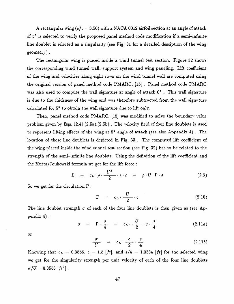
A rectangular wing (s/c = 3.56) with a NACA 0012 airfoil section at an angle of attack
of 50 is selected to verify the proposed panel method code modification if a semi-infinite
line doublet is selected as a singularity (see Fig. 31 for a detailed desciption of the wing
geometry) .
The rectangular wing is placed inside a wind tunnel test section. Figure 32 shows
the corresponding wind tunnel wall, support system and wing paneling. Lift coefficient
of the wing and velocities Mong eight rows on the wind tunnel wall are computed using
the original version of panel method code PMARC, [15] . Panel method code PMARC
was also used to compute the wall signature at angle of attack 0 ° This wall signature
is due to the thickness of the wing and was therefore subtracted from the wall signature
calculated for 5 o to obtain the wall signature due to lift only.
Then, panel method code PMARC, [15] was modified to solve the boundary value
problem given by Eqs. (2.4),(2.5a),(2.5b). The velocity field of four line doublets is used
to represent lifting effects of the wing at 5 o angle of attack (see also Appendix 4) . The
location of these line doublets is depicted in Fig. 33 . The computed lift coefficient of
the wing placed inside the wind tunnel test section (see Fig. 32) has to be related to the
strength of the semi-infinite line doublets. Using the definition of the lift coefficient and
the Kutta/Joukowski formula we get for the lift force :
U 2
_.s.c = p.U.F-s (2.9)L = eL • fl •
So we get for the circulation F :
F =U
cL • --. c (2.10)2
The line doublet strength _ of each of the four line doublets is then given as (see Ap-
pendix 4) :s U s
cr = C. --_ = CL" --_'c" T (2.11a)
or
6 r c s
= eL" --. -- (2.115)U 2 4
Knowing that CL = 0.3556, c = 1.5 [ft], and s/4 = 1.3334 [ft] for the selected wing
we get for the singularity strength per unit velocity of each of the four line doublets
a /U = 0.3556 [ft 2] .
47
The wing can now be replaced by four line doublets of strength 0.3556 [ft 2] and
velocities are again computed on eight rows using the modified version of the panel method
code.
Figure 34 compares dimensionless velocities on the wind tunnel wall of both calcula-
tions at Row 8. Velocities due to lift effects show excellent agreement to verify the proposed
panel method code modifications if semi-infinite line doublets are used to represent lift of
a wing.
Summary
A three-dimensional panel method code was modified to calculate the flow field of
a singularity placed inside a wind tunnel test section. The modification was verified by
replacing a Rankine body by a point source and point sink and by replacing a rectangular
wing at 50 angle of attack by four line doublets. Corresponding flow field solutions compare
favorably in both cases. The panel method code modification will work with no restrictions
if a point source or point sink is selected as a singularity. However, boundary conditions
have to be modified carefully if a horseshoe vortex or semi-infinite line doublet is selected as
this type of singularity intersects outflow panels of the internal flow geometry and therefore
requires a numerical integration of the corresponding point doublet solution.
48
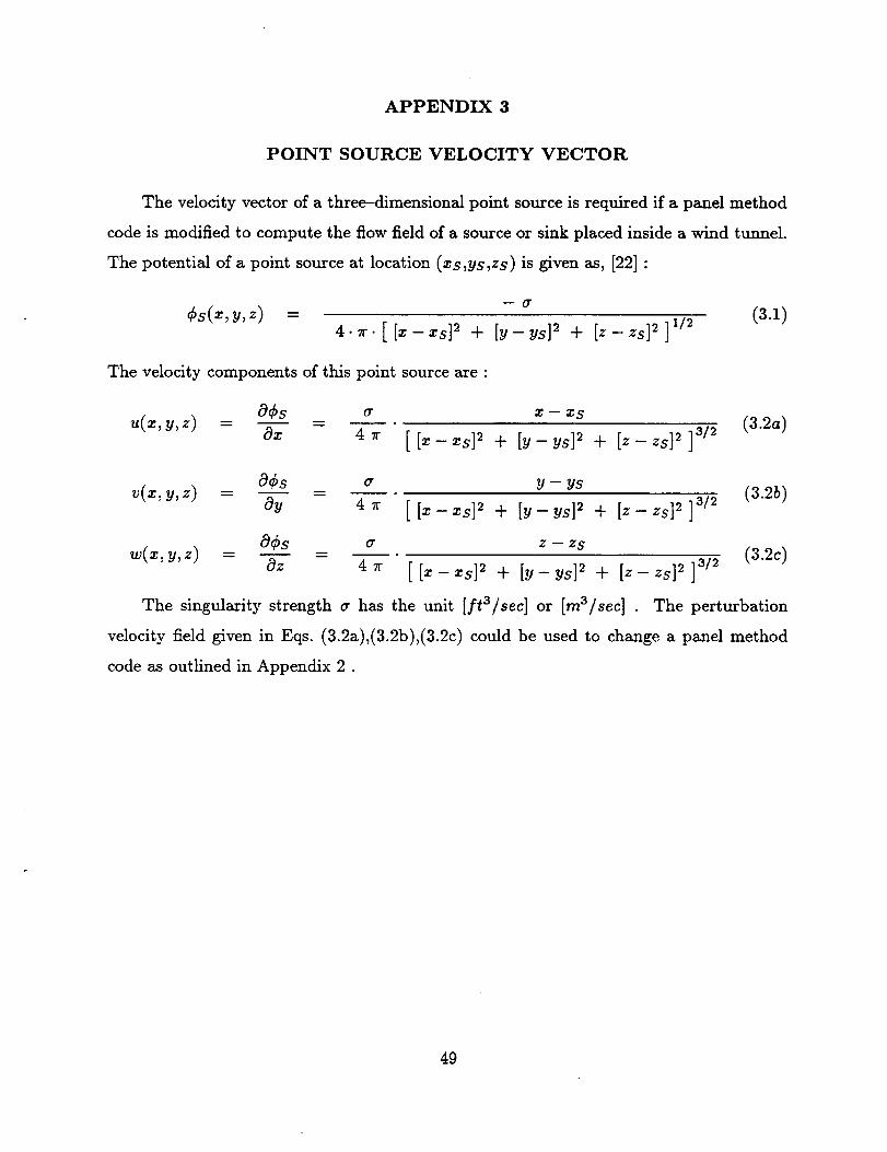
APPENDIX 3
POINT SOURCE VELOCITY VECTOR
The velocity vector of a three-dimensional point source is required if a panel method
code is modified to compute the flow field of a source or sink placed inside a wind tunnel.
The potential of a point source at location (zs,Vs,zs) is given as, [22] :
Cs(x, y, z) = - o"4. _ [ [=- xs]2 + [y- ys]2 + [z- zs]2 ],/2 (3.1)
The velocity components of this point source are :
_S Or X -- XS
u(z,y,z) = 69x = 4 7r [ [z-- xS] 2 + [y -- ys] 2 + [z-- zs] 2 ]3/2 (3.2a)
a&s a y - ysv(x_ y_z) (3.2b)
ay- 47r [[x-zs] 2 + [y-ys] 2 + [z-zs] 213/2
_¢S _ z -- zS
w(=,y,z) = az = 4_ [[=_x_]2 + [y_ys]2 + [z-z_]213/2 (3.2c)
The singularity strength cr has the unit [ft3/sec] or [mZ/sec] . The perturbation
velocity field given in Eqs. (3.2a),(3.2b),(3.2c) could be used to change a panel method
code as outlined in Appendix 2 .
49

50
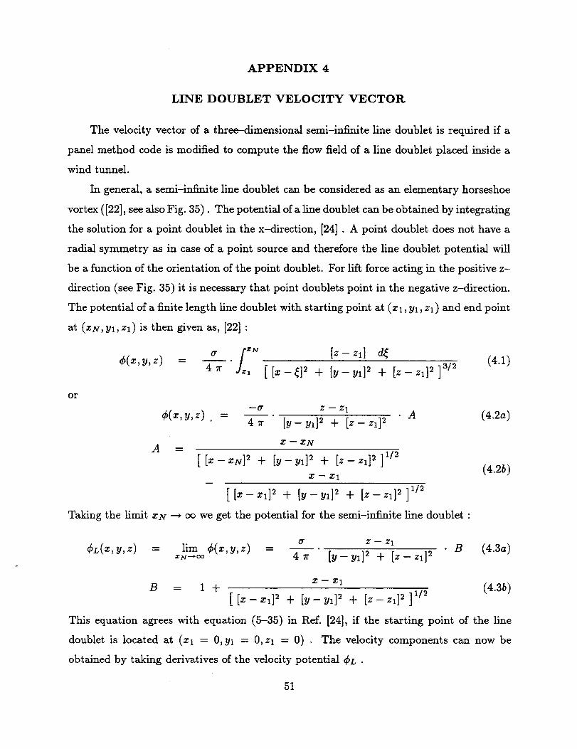
APPENDIX 4
LINE DOUBLET VELOCITY VECTOR
The velocity vector of a three-dimensional semi-infinite line doublet is required if a
panel method code is modified to compute the flow field of a line doublet placed inside a
wind tunnel.
In general, a semi-inflnite line doublet can be considered as an elementary horseshoe
vortex ([22], see also Fig. 35). The potential of a line doublet can be obtained by integrating
the solution for a point doublet in the x-direction, [24] . A point doublet does not have a
radial symmetry as in case of a point source and therefore the line doublet potential will
be a function of the orientation of the point doublet. For lift force acting in the positive z-
direction (see Fig. 35) it is necessary that point doublets point in the negative z-direction.
The potential of a finite length line doublet with starting point at (zl, Yl, zl ) and end point
at (ZN, Yl, zl) is then given as, [22] :
[z- zl]¢(z, y, z) = 4-"7" Jz,
(4.1)
or
[ [X--_12 2y [y__yl]2 2V [Z-- Z II 2 ]3/2
--0" Z -- Z 1
_b(z,y,z) . = 4 _r [y- yl] 2 + [z- zl] 2 A (4.2a)
A
X -- XN
[ 2 + [y- 12 + [z-z112X -- X 1
[ [X-- Xl] 2 "4- [y-- yl] 2 "4- [Z--Zl] 2 ]1/2
Taking the limit zN _ o0 we get the potential for the semi-infinite line doublet :
(4.2b)
¢L(z,y,z) = lim ¢(z,y,z) -- a z-- zl_N--.oo 4----'_ " [y- yl] 2 + [z -- zl] 2 B (4.3a)
B = 1 + z- zl (4.3b)
[ [X-- Xl] 2 "3t- [y-- yl] 2 _t. [Z-- Zl] 2 ]1/2
This equation agrees with equation (5-35) in Ref. [24], if the starting point of the line
doublet is located at (zl = 0, yl = 0, zl = 0) . The velocity components can now be
obtained by taking derivatives of the velocity potential qgL .
51
In the x-direction we get :
U(X y, Z) "-- _¢L -- dr Z -- Z 1
' az -- 4_" [[Z-Zl] 2 + [y-yl] 2 + [z-zl] 213/2 (4.4)
In the y-direction we get :
O_L _ -dr [y- yl]. [z- zl]v(x,y,z) = oy - 4_ [y_y,]2 + [z-_,]2 c (4.5a)
2 • B z-z1
C = [y-yl] 2 + [z-zl] 2 + [[z-z1] 2 + [y-y1] 2 + [Z-Zl] 2]a/2 (4.5b)
In the z-direction we get :
aCL a 1
w(z,y,z) = Oz = 4 r [y-- yl] 2 + [z -- zl] 2 D (4.6a)
D = [Y- yl]2 - [z- Zl] 2 . B[y- _,]_ + [z- Zl]2
[z- zl]" [z - Zl] 2 (4.6b)
[ [_- _,]_ + [_- y,]_ + [z- z,]_]_z_The calculation of the flow field of a semi-infinite line doublet located inside a wind
tunnel of constant cross-sectional area is difficult if a modified version of panel method
code PMARC is used (see Appendix 2) . The line doublet intersects the exit plane of the
paneled wind tunnel geometry and can cause convergence and accuracy problems.
Fortunately, it is possible to calculate the flow fieht of a line doublet in a wind tunnel
of constant cross-sectional area by integrating the flow field of the panel method code
solution of a point doublet in the streamwise direction. The line doublet flow field solu-
tion is obtained by shifting and superimposing corresponding point doublet solutions (see
Fig. 36a).
In general, the potential of a semi-infinite line doublet (Eq. (4.1) ; ZN >> zl) can be
approximated using numerical integration. We get then :
N
CL(z,y,z) _ _ _pD(z,y,z; :rk )" /X_r (4.7a)t;=1
CpD(;r,y,Z; T, k )dr Z -- Zl
(4.7b)4 [ [_- _]_ + [_- y,]_ + [_- Zl]_]_/_11"
52
zk = zl + (k - 1).Az ; zN >> zl
where Az is the step size of the integration. The perturbation velocities of the line doublet
can now be approximated as :
N 0
u(x,y,z) ,._ Az. E _ dZpD(x,y,z; xk ) (4.Sa)k--1
g 0
k=l
iv c9
w(x,y,z) _, Ax. E "_z dppD(x,y,z; xk ) (4.8c)k=l
where
0
a--_6pD(.,y,z; *_ )rr (-3). [x -- xk]-[z-- Zl]
4_r [[z-rk] 2 + [y--y1] 2 + [z--zl] 215/2 (4.9a)
0 a (-3). [y- Yl]"[z- zl] (4.9b)o_ 4".(,,_,z; _ ) = 4 _ [[_-_,]_ + b-y1] 2 + [z-zl]2 ]_/_
o ¢ [_- _]_ + [y- y_]_- 2. [z- z_]_0---_C_pD(x,y,z; xk ) = 4---'_" [ [z- zk]2 + [y- yl]2 + [z-- zl]2 ]5/_ (4.9c)
For a wind tunnel of constant cross-sectional area a streamwise shift of the flow field
solution of a point doublet located at (zl, y_, z_) is possible (see Fig. 36b). Therefore
Eqs. (4.8a), (4.8b), (4.8c)only require the calculation of dppD(X,y,z; X 1 ) aS the following
relationships apply :
0 0
0--;Ce.(.,y,z; _k ) = 0--;¢Po(*-[k-1]a_,_,z; .] ) (4.10_)
0 0_n dflPD(_,Y,Z; Xk ) "-" c,_ dPPD(T' -- []¢-- ].]Ax,y,z; Xl ) (4.10b)yo yu
0 0
a---z ¢pD(x,y,z; xk ) = Cg-'-'zCpD(x--[k--1]Ax,y,z; a:l ) (4.10c)
The numerical integration defined by Eqs. (4.8a), (4.8b), (4.8c) has to be done care-
fully. Integration error due to the fact that the numerical solution of a point doublet flow
field is not perfectly antisymmetric (see Eq. (4.9a)) or symmetric (see Eqs. (4.9b),(4.9c))
53
relative to its x-coordinate xk has to be avoided. This can be done by considering, e.g.,
the numerical solution upstream (x < xk) of the point doublet as exact and imposing the
following conditions on the downstream part (x > x_) of the perturbation velocities :
u(x,y,z) - - u(xk-Ix- xk],y,z) ; x > x_ (4.11a)
v(x,y,z) = ; • > (4.11b)
w(x,y,z) = w(zk -[x- zkl,y,z) ; z > xk (4.11c)
Unfortunately, the point doublet and therefore also the semi-infinite line doublet does
not have a radial symmetry. However, the velocity vector of a point or line doublet not
pointing in the negative z-axis direction can easily be found by applying a coordinate
system rotation. A rotation angle 7" related to the directional property of the line doublet
is introduced as depicted in Fig. 37.
The relationship of coordinates and velocities between the line doublet fixed coordinate
system (x,y,z) and reference coordinate system (x',y',z') is depicted in Fig. 37 . The
rotation angle direction is defined such that the lift force caused by the semi-infinite line
doublet points in the positive y'-axis if the line doublet is rotated by +900 . In this
case we get for the transformation of coordinates from r,he reference coordinate sytem, i.e.
(z',y',z'), to coordinates in the line doublet fixed coordinate system (x,y,z) :
x - x' (4.12a)
y = y'.cos_" - z'.sinr (4.12b)
z = y'.sin_" + z'.cosr (4.12c)
The velocities components (u,v,w) are computed i:_ the line doublet fixed coordinate
system. Finally it is necessary to back-transform thes_ velocity components to the refer-
ence coordinate system. We get then :
u I = u (4.13a)
v' - v- cos r + w. :_in r (4.13b)
54
w' = - v.sinr + w.cosv (4.13c)
The singularity strength _r has the unit [ft3/sec] or [m3/sec] . The perturbation
velocity field given in Eqs. (4.8a),(4.8b),(4.Sc) could be used to change a panel method
code as outlined in Appendix 2 .
55
56
APPENDIX 5
CALCULATION OF THE LINE DOUBLET STRENGTH
In general, it is possible to compute the strength of line doublets representing lifting
effects of art aircraft by using lift and pitching moment measurements recorded during a
wind tunnel test (see Ulbrich and Steinle,[7] ).
Assuming that the lifting surfaces of the wing and tail of an aircraft model are dis-
cretized by using equally spaced line doublets along the 1/4-chord line of the wing and
tail we get for the total lift and pitching moment (see also Fig. 38) :
L - ELw(i) + y_L,(j) (5.1)
i=I j=l
P = -- + -- l (5.2)"= ]=1
where L_(i) and L,(j) are the lift contributions of the line doublets of the wing and tail.
Similar to Eqs. (2.9) and (2.11), the Kutta/Joukowstd formula may be used to connect
a lift force to a line doublet strength. The application of the Kutta/Joukowski formula in
a wind tunnel requires the calculation of the product poo • Uoo where poo is the free-stream
density and U_o is the free--stream velocity at the location of the aircraft model. A first
order approximation of the product p_- Uoo may be obtained by applying wall interference
corrections to the measured reference density prel and reference velocity Uref at a model
reference station (see Eqs. (5.78) and (5.82) in Ref. [10]). We then get:
poo'Uoo _ prel'Ure," [1 -t- ¢'(1 --M_2el )] (5.3a)
The Kutta/Joukowski formula may now be written as :
L,_(i) = poo " Uoo " cr_o(i) ,_ P, ef " Vr,l " [ 1 + _ . ( 1 - M_ l ) ].a_(i) (5.3b)
L,(j) = poo " Voo " _;(j) ,_ Pref " U, ef " [ I + e" ( 1 - M;2el ) ]. g;(j) (5.3c)
Introducing singularity weights w_ (i), w,(j), and discrete line doublet span As_, As,
on the wing and tail we get for the singularity strength :
_(i) = F_ . As,_ . w_(i) (5.4a)
57
_;(j) = rt. As,. wt(j) (5.45)
The circulation F_ and F_ are the only unknowns in Eqs. (5.1) and (5.2) if line doublets
weights are specified by the user. The weights may represent, e.g., elliptic lift distribution
along the wing and tail of an aircraft model. Experimental or CFD solutions of the true
lift distribution may also be used to determine weights (see also NACA Report No. 921,
[25]). Combining Eqs. (5.1) to (5.45) we get:
L- Fto • oq -t- Ft- or2 (5.5a)
where
P= Fto • 171 -t- Ft- 132 (5.5b)
1"I w
_1 = Asto._wto(i) (5.6a)i--1
"1%t
,_ = A,,t._ w,(j) (5.6b)j=l
131 = Asto •
/32 = Ast •
Equations (5.5a) and (5.5b) are a 2
easily for Fto and Ft :
ww(i).[zm,. - zto(i)] (5.7a)*_.
_,(j). [=_,. - =t(j) ] (5.7b)j=l
x 2 linear system of equations which can be solved
Fto = 1 L-132 - P'a2 (5.8a)
Ft = 1 (-L)-131 q- P'_I (5.85)
Finally, the singularity strength is obtained by applying Eqs. (5.4a) and (5.4b).
The line doublet strength has to be compatible with non-dimensionalized perturba-
tion velocities used in the panel method code computation of the wind tunnel and wall
interference flow field (see Eq. (25) and Appendix 2). Correct units for velocity, density,
58
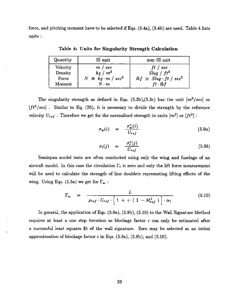
force, and pitching momenthave to be selected if Eqs. (5.4a), (5.4b) are used. Table 4 lists
units :
Table 4: Units for Singularity Strength Calculation
Quantity SI unit non-SI unit
Velocity
Density
Force
Moment
N
Tt_ / $eC
- kg. m / sec2
N.m
lbf
fg / $CC
Slug / ft 3
-- Slug. ft / sec _
ft . lb f
The singularity strength as defined in Eqs. (5.3b),(5.3c) has the unit [rn3/sec] or
[ft3/sec] . Similar to Eq. (25), it is necessary to divide the strength by the reference
velocity Urey • Therefore we get for the normalized strength in units [rn 2] or [ft 2] :
a_(i) = a*(i) (5.9a)
at(j) = a;(j) (5.9b)U_f
Semispan model tests are often conducted using only the wing and fuselage of an
aircraft model. In this case the circulation Ft is zero and only the lift force measurement
will be used to calculate the strength of line doublets representing rifting effects of the
wing. Using Eqs. (5.5a) we get for F_ :
Lr_ = (5.10)
p_1"Ur_f" [1 + e.(1 -M_ 1 )] "al
In general, the application of Eqs. (5.8a), (5.8b), (5.10) to the Wall Signature Method
requires at least a one step iteration as blockage factor e can only be estimated after
a successful least squares fit of the wall signature. Zero may be selected as an initial
approximation of blockage factor e in Eqs. (5.8a), (5.8b), and (5.10).
59
60
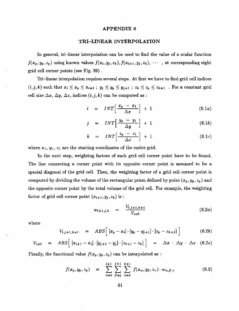
APPENDIX 6
TRI-LINEAR INTERP OLATION
In general, tri-linear interpolation can be used to ffud the value of a scalar function
f ( xp , yp , zp ) using known values f (z¢ , yj , zk ) , f (zi + l , yj , z_ ) , ... , at corresponding eight
grid cell corner points (see Fig. 39) .
Tri-linear interpolation requires several steps. At first we have to find grid cell indices
(i,j,k) such that z_ < zp _< zi+l ; yj <_ yp <_ Yj+I ; zk <_ zp <_ zk+l • Fora constant grid
cell size Az, Ay, Az, indices (i,j, k) can be computed as :
i = INT zp - zl ]Ax + 1 (6.1a)
INT yp - y_ 1J + 1 (6.1b)
k = INT[ ZpAz- zl]] + 1 (6.1c)
where Xl, Yl, Zl are the starting coordinates of the entire grid.
In the next step, weighting factors of each grid cell corner point have to be found.
The line connecting a corner point with its opposite corner point is assumed to be a
spacial diagonal of the grid cell. Then, the weighting factor of a grid cell corner point is
computed by dividing the volume of the rectangular prism defined by point (xv, yp, zp) and
the opposite corner point by the total volume of the grid cell. For example, the weighting
factor of grid cell corner point (zi+l, yj, zk) is :
TVi'J+l'k +1 (6.2a)Wi+ l,j,k = Ycell
where
V/,j+l,k+l = ABS[ [T,p -- Zi] " [yp -- Yj+I]" [Zp " Zk+l] ] (6.2b)
V_n = ABS[ [xi+l - xi] . [yj-t-1 - yj] " [Zk-t-1 -- Zk] ] : AT. • Ay " AZ (6.2C)
Finally, the functional value f(xp, yp, zp) can be interpolated as :
i+1 j+l k+l
f(z,,yp,zp) = _ _ _ f(xc,,y_,z._).w,_,_,._ (6.3)
a=i fl=j "y=k
61
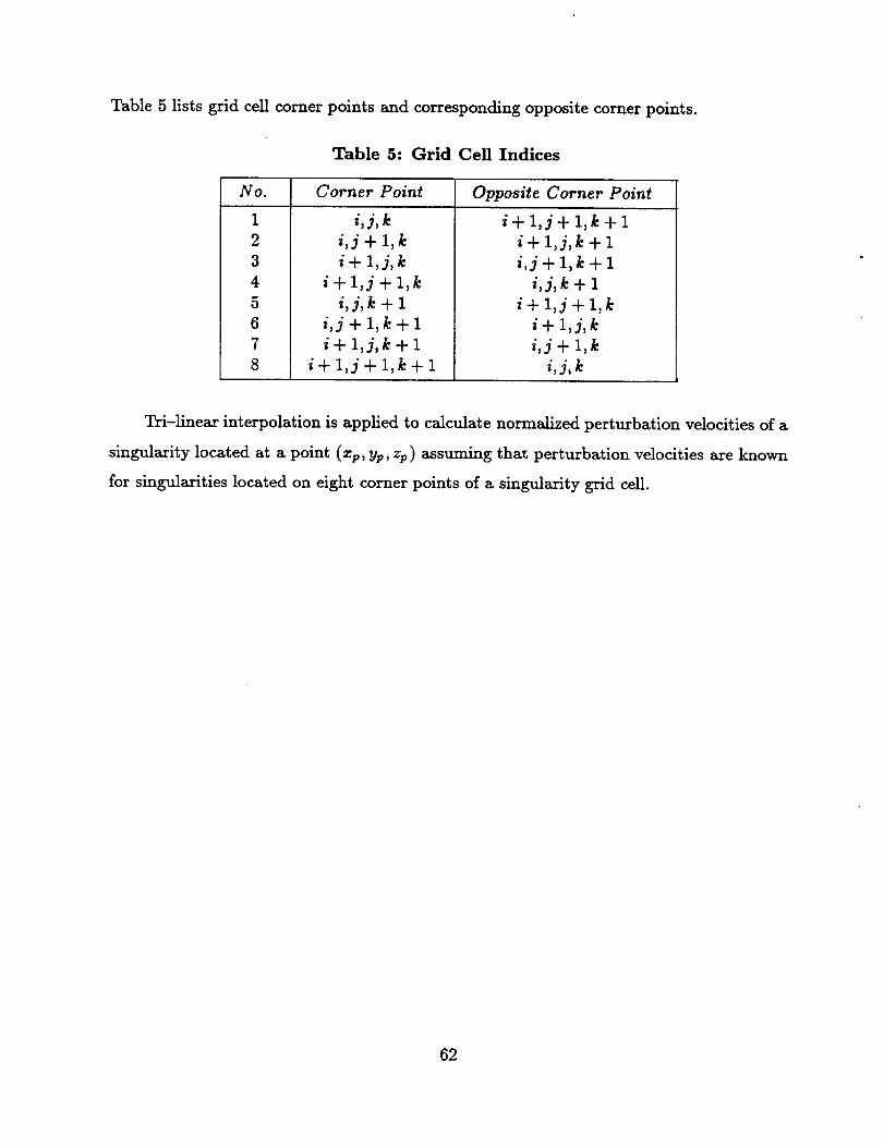
Table 5 lists grid cell comer points and corresponding opposite comer points.
Table 5: Grid Cell Indices
No. Corner Point Opposite Corner Point
1
2
3
4
5
6
7
8
i, j, ki,j + l,k
i+ 1,j,k
i + l,j + l,k
i,j,k+l
i,j+l,k+l
i + l,j,k + l
i + l,j + l,k + l
i+l,j+l,k+l
i + l,j,k + l
i,j+l,k+l
i, j, k + 1
i+l,j+l,k
i+ 1,j,k
i,j+l,k
i, j, k
Tri-linear interpolation is applied to calculate normalized perturbation velocities of a
singularity located at a point (xp, yp, zp) assuming that perturbation velocities are known
for singularities located on eight comer points of a singularity grid cell.
62
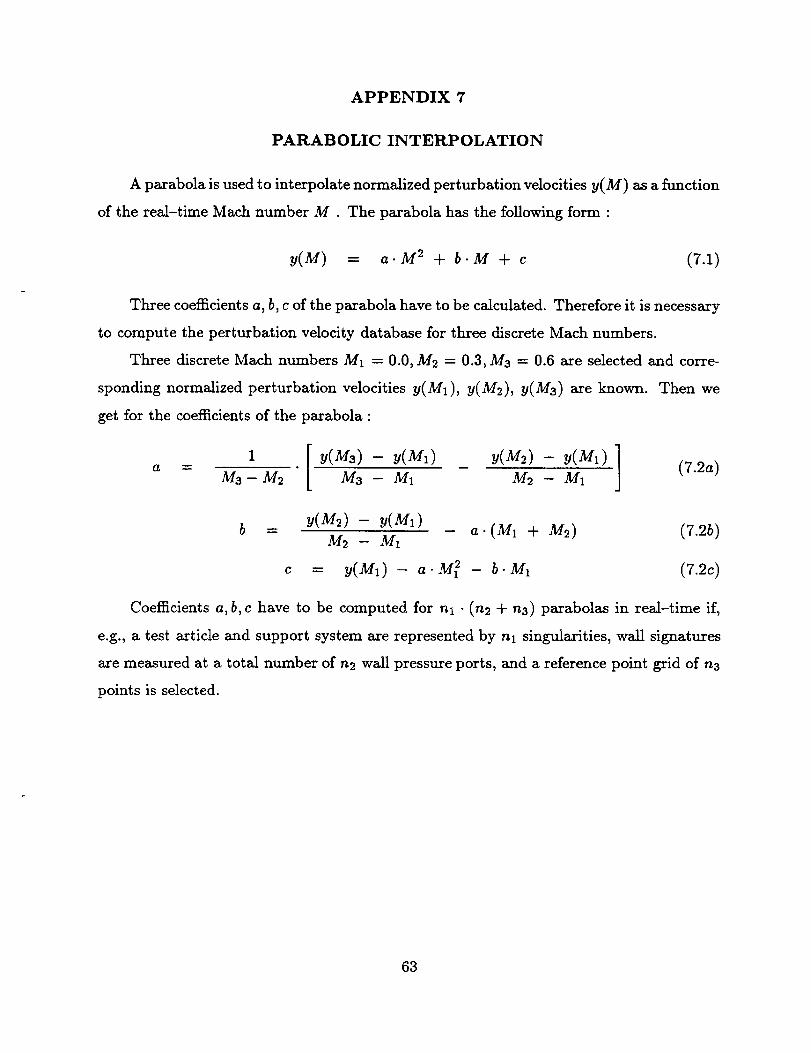
APPENDIX 7
PARABOLIC INTERPOLATION
A parabola isused to interpolatenormalized perturbation velocitiesy(M) as a function
of the real-time Mach number M . The parabola has the followingform :
y(M) = a.M 2 -{- b.M + c (7.1)
Three coefficients a, b, c of the parabola have to be calculated. Therefore it is necessary
to compute the perturbation velocity database for three discrete Mach numbers.
Three discrete Mach numbers M1 = 0.0, M2 = 0.3, M3 = 0.6 are selected and corre-
sponding normalized perturbation velocities y(M1), y(M2), y(M3) are known. Then we
get for the coefficients of the parabola :
a ---
M3- M2
y(M3) - y(M1) y(M2)- y(M1)
M3 - M1 M2 - M1(7.2a)
b -" y(M2)- y(M1) - a.(M1 -b M2) (7.2b)M2 - M1
c = y(M1) - a. M_ - b. M1 (7.2c)
Coefficients a, b, c have to be computed for nl • (n2 + n3) parabolas in real-time if,
e.g., a test article and support system are represented by nl singularities, wall signatures
are measured at a total number of n2 wall pressure ports, and a reference point grid of n3
points is selected.
63
64
APPENDIX 8
OPTIMIZATION OF THE SINGULARITY LOCATION
The wall signature method calculates wall interference corrections based on a singu-
larity representation of the test article and the support system. The wind tunnel test
engineer has to specify the initial location of these singularities using simple rules. For
example, sources and sinks representing the fuselage volume should be located along the
fuselage axis such that they represent a Rankine body approximation of fuselage volume
effects, line doublets should be distributed along the 1/4-chord line of lifting surfaces, and
sources related to separation wake effects should be located at points where separation is
likely to occur during a test.
The initial singularity representation is not unique as the test engineer has to specify
the singularity location. However, it is possible to make the singularity location unique by
minimizing the standard deviation of the least squares fit as a function of the singularity
location.
An efficient optimization can only be achieved if the total number of independent
variables of the minimization, i.e. the coordinates of each singularity, is reduced to a
reasonable limit. It is also necessary to restrict the direction of change of the singularity
coordinates.
During the support system calibration three groups of singularities exist, i.e., sources of
the support system volume, sinks of the support system volume, and sources of the support
system wake. Therefore it is possible to reduce the number of independent variables
down to three, if the relative distances of the singularities of each group is kept constant
during the optimization. The direction of change of the optimization is defined by the
line connecting the first source and the first sink of singularities representing the support
system volume.
Similarly, during the wind tunnel test of a test article five groups of singularities
exist, i.e., sources of the fuselage volume, sinks of the fuselage volume_ and sources of the
wing separation wake, line doublets of the wing, and line doublets of the tail. Therefore
the number of independent variables can be reduced to five, if the relative distances of
65
the singularities of each group is kept constant during the optimization. In this case the
direction of change of the optimization is defined by the line connecting the first source
and the first sink of singularities representing the fuselage vohune. Assuming that the
1/4-chord line of the wing and tail are ideal locations for line doublets of the wing and
tail it is even possible to reduce the ntunber of independent variables to three.
An optimization algorithm based on the Method of Steepest Decent has been included
in the real-time software package of WICS (see also Ref. [261).
66
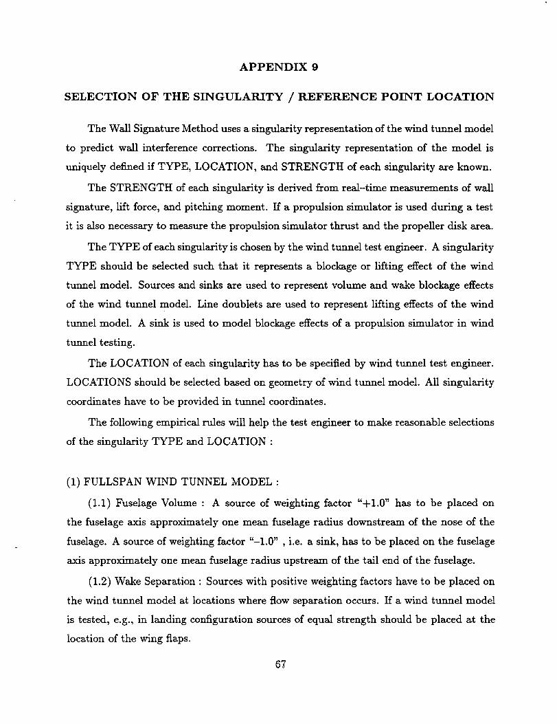
APPENDIX 9
SELECTION OF THE SINGULARITY / REFERENCE POINT LOCATION
The Wall Signature Method uses a singularity representation of the wind tunnel model
to predict wall interference corrections. The singularity representation of the model is
uniquely defined if TYPE, LOCATION, and STRENGTH of each singularity are known.
The STRENGTH of each singularity is derived from real-time measurements of wall
signature, lift force, and pitching moment. If a propulsion simulator is used during a test
it is also necessary to measure the propulsion simulator thrust and the propeller disk area.
The TYPE of each singularity is chosen by the wind tunnel test engineer. A singularity
TYPE should be selected such that it represents a blockage or lifting effect of the wind
tunnel model. Sources and sinks are used to represent volume and wake blockage effects
of the wind tunnel model. Line doublets are used to represent lifting effects of the wind
tunnel model. A sink is used to model blockage effects of a propulsion simulator in wind
tunnel testing.
The LOCATION of each singularity has to be specified by wind tunnel test engineer.
LOCATIONS should be selected based on geometry of wind tunnel model. All singularity
coordinates have to be provided in tunnel coordinates.
The following empirical rules will help the test engineer to make reasonable selections
of the singularity TYPE and LOCATION :
(1) FULLSPAN WIND TUNNEL MODEL :
(1.1) Fuselage Volume : A source of weighting factor "+1.0" has to be placed on
the fuselage axis approximately one mean fuselage radius downstream of the nose of the
fuselage. A source of weighting factor "-1.0" , i.e. a sink, has to be placed on the fuselage
axis approximately one mean fuselage radius upstream of the tail end of the fuselage.
(1.2) Wake Separation : Sources with positive weighting factors have to be placed on
the wind tunnel model at locations where flow separation occurs. If a wind tunnel model
is tested, e.g., in landing configuration sources of equal strength should be placed at the
location of the wing flaps.
67
(1.3) Wing : The wing spanis divided into equal sizewing span increments. Oneline
doublet is assignedto each wing spanincrement. Line doublet starting points are placed
where the 1/4 chordline of the wing and the middle of eachwing span increment intersect.
(1.4) Tail : The tail span is divided into equal size tail span increments. One line
doublet is assignedto each tail span increment. Line doublet starting points are placed
where the 1/4 chord line of the tail and the middle of eachtail span increment intersect.
(1.5) Propulsion Simulator : A sourceof weighting factor "-1.0" , i.e. a sink, is placed
at the centerof the propeller if a turboprop engine is simulated; a sink is placed halfway
between the compressorand turbine if a turbojet or turbofan engine is simulated.
(2) SEMISPAN WIND TUNNEL MODEL :
(2.1) FuselageVolume : A sourceof weighting factor "+1.0" has to be placed on
the fuselageaxis approximately one mean fuselageradius downstream of the noseof the
fuselage. A sourceof weighting factor "-1.0" , i.e. a sink, has to be placedon the fuselage
axis approximately one mean fuselageradius upstream of the tail end of the fuselage.
The z-coordinate of the sourceand sink of the semispanmodel fuselagedoesnot have to
be specified. The Wall Interference Correction System (WICS) of the NASA Ames 12ft
PressureWind Tunnel (PWT) implicitly assumesthat their z-coordinate is identical with
the z-coordinate of the imageplane surface.
(2.2) Wake Separation : Sourceswith positive weighting factors have to be placedon
the wind tunnel model at locations whereflow separation occurs. If a wind tunnel model
is tested, e.g., in landing configuration sourcesof equal strength should be placedat the
location of the wing flaps.
(2.3) Wing : The wing semispanis divided into equaisizewing spanincrements. One
line doublet is assignedto each wing span increment. Line doublet starting points are
placed where the 1/4 chord line of the semispanwing and the middle of each wing span
increment intersect.
(2.4) Propulsion Simulator : A sourceof weighting factor "-1.0" _i.e. a sink, is placed
at the centerof the propeller if a turboprop engine is simulated; a sink is placed halfway
betweenthe compressorand turbine if a turbojet or turbofan engine is simulated.
68
(3) REFERENCE POINTS :
WICS computesmean wall interferencecorrections for sets of referencepoints. The
test engineerhas to specify thesesets of referencepoints in the tunnel coordinate system.
WICS allows the test engineer to specify up to 10 independent sets of referencepoints.
Setsof referencepoints can be specifiedalong the fuselageaxis and along the 3/4 chord
line of the wing or tail.
A simple Expert Systemshouldbe designedin the future that assiststhe test engineer
in the selectionof the singulal"itylocation and weighting factors.
69
70
APPENDIX 10
BLOCKAGE EFFECT OF A POWERED WIND TUNNEL MODEL
The correct simulation of flow interference effects between the aircraft fuselage, the
wing, and the engine cowling during a wind tunnel test requires the installation of a propul-
sion simulator in a wind tunnel model. The blockage correction caused by a propulsion
simulator has to be estimated if a significant amount of thrust is produced.
In general, a propulsion simulator is operated as a small propeller. A point doublet
pointing in the streamwise direction may be used to estimate propulsion simulator blockage
effects during a wind tunnel test, [22] . A more accurate modeling of blockage effects may
be obtained if a semi-infinite line doublet pointing in the streamwise direction is used, [27] .
The velocity potential of a semi-infinite line doublet with a starting point at (zl, yl, zl ) is
given as, [22]:
- a lim ....
CLD(Z,y,z) -- 47r ==--.oo , [[z__] 2 + [y_yl] 2 + [z_zl] 213/2 (10.1)
It can be shown that the velocity potential defined in Eq. (10.1) is identical with the
velocity potential of a sink located at (xl, yl, zl) (see Eq. 3.1) :
O"
CLD(X,y,z) = --¢S(X,y,z) = 4 _r
1
[[_-_1] 2 + [y-yl]2 + [z-zip]l/_ (10.2)
Location and strength of this sink have to be specified. It is reasonable to place the sink
at the center of the propeller or compressor disk of the propulsion simulator. The sink
strength a may be related to the propulsion simulator thrust Tp, propeller disk area S,
free-stream velocity Uoo, and free-stream density pco by applying an approximate solution
of the flow around the ideal propeller given by Koning, [6] . In wind tunnel testing, free--
stream velocity and density have to be estimated by applying blockage corrections to the
measured reference velocity U,e! and reference density p, ej', i.e. Uoo _ U-el (1 + e) and
poo _ pr_! (1 - c M]_I) (see Eqs. (5.78) and (5.82) in aef.[10]) . Then, we get for the
propulsion simulator sink strength :
F/ 2. Tp 1/J -- _T_f _ ( 1-[- _)/ (10.3)
% = S. LvU f'(1 +e) 2 + p,.e.f.(1-e M_._I).S J
71
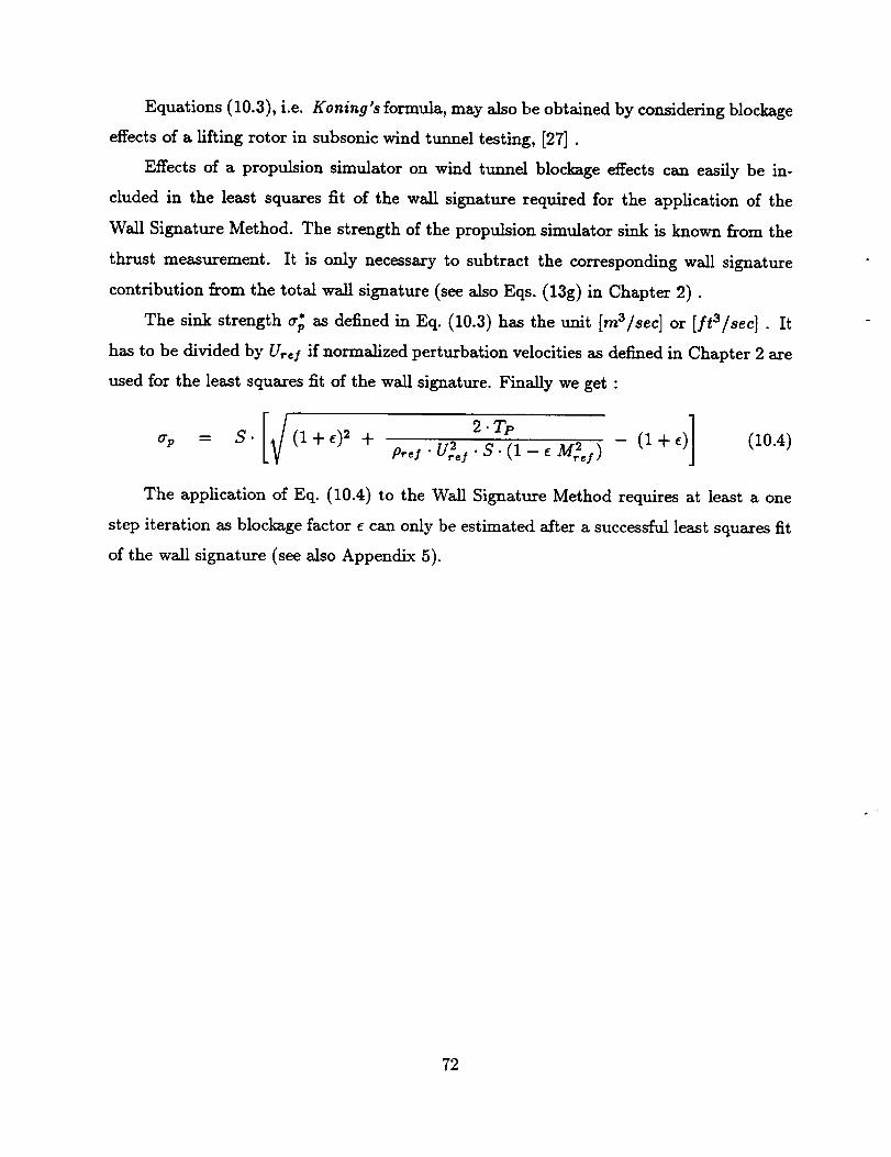
Equations (10.3), i.e. Koning's formula, may also be obtained by considering blockage
effects of a lifting rotor in subsonic wind tumad testing, [27] .
Effects of a propulsion simulator on wind tunnd blockage effects can easily be in-
eluded in the least squares fit of the wall signature required for the application of the
Wall Signature Method. The strength of the propulsion simulator sink is known from the
thrust measurement. It is only necessary to subtract the corresponding wall signature
contribution from the total wall signature (see also Eqs. (13g) in Chapter 2).
The sink strength _,; as defined in Eq. (10.3) has the unit [m3/sec] or [ft3/sec]. It
has to be divided by U,._I if normalized perturbation velocities as defined in Chapter 2 are
used for the least squares fit of the wall signature. Finally we get :
[_ 2.Tp -(1+ _)] (10.4)_, = S. (1+,) 2 + p,,_._Lj.s.(I_,MLj )
The application of Eq. (10.4) to the Wall Signature Method requires at least a one
step iteration as blockage factor e can only be estimated after a successful least squares fit
of the wall signature (see also Appendix 5).
72
APPENDIX 11
QUALITY CHECK OF THE LEAST SQUARES FIT
The Wall Signature Method uses a linear least squares fit of the difference between
wall signature and corresponding wall pressure port calibration to predict blockage effects
of a test article. In practical applications the facility hardware cannot guarantee that good
pressure measurements are recorded on all wall pressure ports at all times. However, not
all pressure measurements are required to compute a blockage correction of the test article.
Therefore an efficient implementation of a wall interference correction system based on the
Wall Signature Method has to check measurements on each wall pressure port.
Studies using experimental data have shown that a four-step quality check of the
least squares fit is sufficient to identify unacceptable wall signature measurements without
rejecting too many data points. Wall signatures obtained during the empty tunnel or
support system calibration have to be inspected separately. They are used to remove
orifice error, wall divergence, and wall boundary layer displacement effects.
The proposed quality check of the difference between the real-time and calibrated
wall signature is done as follows (see also Fig. 40) :
CHECK 1 : WALL SIGNATURE DIFFERENCE MAGNITUDE
The absolute value of the wall signature difference is computed for each wall pressure
port. A port is rejected, i.e. its port flag is set to zero, if the wall signature difference is
larger than a specified upper bound. This bound is a function of the wind tunnel facility
configuration and data aquisition hardware. An upper bound of 0.1 has been selected for
the NASA Ames 12ft Pressure Wind Tunnel.
CHECK 2 : OUTLIER IDENTIFICATION
The absolute value of the difference between the wall signature difference and its least
squares fit is computed for each wall pressure port. A port is rejected, i.e. its port flag is
set to zero, if this difference is larger than three times the standard deviation of the least
squares fit.
CHECK 3 : STANDARD DEVIATION OF EACH ROW
The standard deviation of each wall pressure port row is computed. A wall pressure
73
port row is rejected, i.e. its wall pressure port flags are set to zero, if the standard deviation
is larger than a specified upper bound. This bound is a function of the wind tunnel
facility configuration and data aquisition hardware. An upper bound of 0.01 (perturbation
velocity) has been selected for the NASA Ames 12ft Pressure Wind Tunnel.
CHECK 4 : WALL PRESSURE PORT NUMBER
The total number of wall pressure ports used for the least squares fit of the wall
signature difference is computed after CHECKS 1 TO 3 are applied. No wall interference
corrections are computed if the total number of wall pressure ports is smaller than a
specified lower limit. The lower limit of wall pressure ports is a function of the wind
tunnel facility. A number of 60 wall pressure ports has been selected as the lower limit of
the NASA Ames 12ft Pressure Wind Tunnel.
74
APPENDIX 12
LINEAR INTERPOLATION OF WALL PRESSURE PORT CALIBRATION
The Wall Signature Method uses a linear least squares fit of the difference between
real-time wall signature and corresponding wall pressure port calibration to determine
blockage effects of a test article. A value of the wall pressure port calibration has to be
found that matches real-time test conditions.
The wall pressure port calibration is usually a function of several independent calibra-
tion variables. It can be a function of the total pressure PT and Mach number M at some
wind tunnel reference station. The wall pressure port calibration can also be a function of
the support system kinematics. In this case calibration variables describing the position
of the support system during the calibration have to be introduced.
An interpolation algorithm has been developed for the WICS software package that
uses linear interpolation to determine the wall pressure port calibration as a function of
real-time test conditions. This algorithm fulfills reliability, performance, and accuracy
requirements of WICS.
The interpolation algorithm is applicable to up to four independent calibration vari-
ables. As an example, a detailed description of this interpolation algorithm for two indepen-
dent calibration variables will be presented below. A detailed description of the algorithm
for three and four independent variables is beyond the scope of the WICS Theory Guide.
In general, a value of the wall pressure port calibration C(X*, Y*) has to be found for
real-time test conditions defined by, e.g., two independent variables X*, Y* . It is assumed
that wall pressure ports are calibrated for discrete combinations of these variables. A
total of "n" discrete values of the first calibration variable Xi were selected. The second
calibration variable ]_,j was changed by keeping the first calibration variable Xi constant.
A total of "re(i)" discrete values of the second calibration variable Y_,j were selected.
Therefore we get the following set of discrete wall pressure port calibrations : C(Xi, Y_,.i)
forl<i<nandl<j<rn(i).
The interpolation of the calibration is done in two steps. At first, calibrations are
interpolated for the second calibration variable Y* . The first calibration variable Xi
75
is kept constant. Comparing Y* and Y_j only one of three possible cases applies (see
Fig. 41a) :
Case i: Y* < _,I
U(X_) = C(X_,_=I) (12.1)
Case 2 : }_,j _< Y* _< _,j+l
c(x_,Y_,j+_) - c(x_,_,_)
Case 3 : Y* > Y_,m(i)
U(x,) = c(x_,Y_,._(_)) (12.3)
Finally, calibrations axe interpolated for the calibration variable X* by using the first
calibration variable X_ and interpolated calibrations C(Xi) . Again, comparing X* and
Xi , only one of three cases applies (see Fig. 41b) :
Case I: X* < X1
C(X*,Y*) = C(X1) (12.4)
Case 2 : Xi <_ X* <_ Xi+l
- v(x,) [x" - x, ] (12.5)C(X',Y') = "C(Xi) + Xi+l - Xi
C(X*,Y*) - C(X,_) (12.6)
Case 3: X* > Xn
Basic ideas and elements of the interpolation algorithm can easily be extended to three
and four independent calibration variables.
Support system wall interference corrections at a reference point grid axe required if
the Wall Interference Correction System of the 12ft PWT is applied to a fullspan model
test configuration (see Fig. 13a) . These corrections are known as a function of calibra-
tion variables. A similar linear interpolation algorithm may be used to interpolate the
corrections for real-time test conditions.
76
APPENDIX 13
SINGULAR VALUE DECOMPOSITION
The numerical method of choice for solving linear least-squares problems, i.e. Eq. (13a)
or Eq. (16a), is the Singular Value Decomposition (SVD) technique, [12]. This robust
numerical technique was selected for the WICS software. The application of the SVD
technique to Eqs. (13a), (16a) can be summarized in three steps :
Step 1 : Rewrite Eq. (13a) or Eq. (16a) as an overdetermined linear system :
A_x2 X2×I = B,_xl (13.1)
Step 2 : Write matrix A as the product of a column-orthogonal matrix U, a diagonal
matrix W with positive or zero elements, and the transpose of an orthogonal matrix V .
Matrices U, W, and V are found using the SVD algorithm. We get :
A,-nx2 = U,-nx2 W2x2 v'r2x2 (13.2)
Step 3 : Determine the solution of the least squares problem by computing the fol-
lowing matrix product :
X2xl = V2x2 W-12x2 u'r2×,, B,_xl (13.3)
It is important to identify elements of the diagonal matrix W, i.e. singular values of
W, that are small. These singular values and their reciprocal will be set to zero if the
least squares problem is iU-conditioned.
77
78
APPENDIX 14
SUPPORT SYSTEM KINEMATICS
In general, it is recommended to compute real-time coordinates of singularities that
represent the support system or the test article if WICS is used to predict wall interference
corrections in the 12ft PWT. This reduces the standard deviation of the least squares fit of
the wall pressure signature and improves the accuracy of computed blockage corrections.
The real-time coordinates of singularities are a function of the kinematics, i.e. the
movement, of the support system or the test article. Three different types of support
systems are presently available for testing in the 12ft PWT, i.e. the Ames Bipod, the High
Angle of Attack Sting, and the Image Plane. Equations describing the movement of these
support systems and of the test article in the tunnel coordinate system (see Figs. 17a,17b)
have to be derived.
Ames Bipod / High Angle of Attack Sting
The kinematics of the Ames Bipod and of the High Angle of Attack Sting in the
tunnel coordinate system are essentially identical, if the roll angle of the High Angle of
Attack Sting is kept at to = 0.0 ° (the more complex case of a non-zero roll angle is
discussed in Appendix 15) . The kinematics may be described by one rotation about the
axis x, = 120.71 [ft], z = 0.0 [ft] and one rotation about the axis x. = 120.71 [ft] ,
y = 0.0 [ft] Angles o_ and f? depicted in Fig. 42a are independent variables that
describe the motion. For a roll angle _ = 0.0 °, angle a may be approximated by the pitch
angle of the wind tunnel model and angle fl may be approximated by the sideslip angle
of the wind tunnel model. Figures 42b and 42c show the connection between angle a,
angle fl, and singularity coordinates. It is assumed that point PI(zl, yl, zl) describes the
initial location of a singularity. After a first rotation about the axis x. = 120.71 [ft] ,
z = 0.0 [ft] the singularity moves to point P2(z2, y2, z2). After a second rotation about
the axis x. = 120.71 [ft] , y = 0.0 [ft] the singularity moves to point P3(z3,y3,z3).
The final position of the singularity at point P3 is known if coordinates x3, Y3, z3 are given
as a function of initial coordinates xl, Yt, zl, the pitch angle a, and the sideslip angle/? .
79
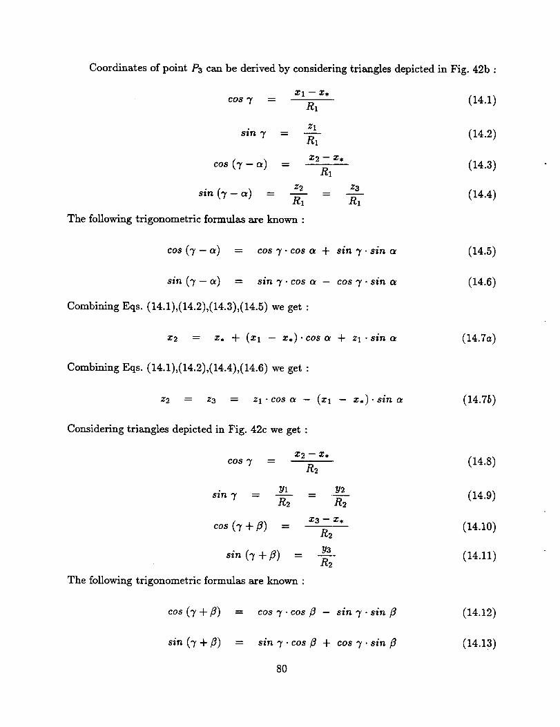
Coordinatesof point P3 can be derived by considering triangles depicted in Fig. 42b :
Xl -- X,
cos 7 = (14.1)R1
Zl
8i. 7 = n---_- (14.2)
co8(7- _) = 2:2- 2:, (14.3)R1
sin (7 - c0 = z2 = z__3_3 (14.4)R1 R1
The following trigonometric fomulas are known :
cos (7 - a) = cos 7"cos ot + sin 7" sin ot (14.5)
sin (7-a) = sin 7" cosa - cos 7" sina
Combining Eqs. (14.1),(14.2),(14.3),(14.5)we get:
(14.6)
2:2 = 2:. + (2:1 - 2:.).cos a + zl.sin a (14.7a)
Combining Eqs. (14.1),(14.2),(14.4),(14.6) we get:
z2 = z3 = zl.cos o_ - (zl - 2:.)'sin ot (14.7b)
Considering triangles depicted in Fig. 42c we get :
2:2 -- 2:*cos 7 = (14.8)
R2
sin 7Yl
R2y2 (14.9)R2
co_(7 + 8)
_i. (7 + 8)
2:3 -- 2:,
R_ (14.10)
Y3 (14.11)R2
The following trigonometric formulas are known :
cos (7+fl) = cos 7" cos fl - sin 7" sin fl (14.12)
sin (7+8) = sin 7" cos fl + cos 7" sin fl (14.13)
8O
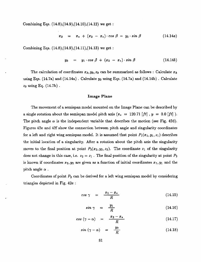
Combining Eqs. (14.8),(14.9),(14.10),(14.12) we get:
x3 = x. + (x2 - x,).cos 13 - Yl" sin ]3 (14.14a)
Combining Eqs. (14.8),(14.9),(14.11),(14.13) we get:
Y3 = Yl .cos 13 + (x2 -- x.).sin 13 (14.14b)
The calculation of coordinates z3, y3, z3 can be summarized as follows : Calculate z3
using Eqs. (14.7a) and (14.14a). Calculate Y3 using Eqs. (14.7a) and (14.14b). Calculate
z3 using Eq. (14.7b) .
Image Plane
The movement of a semispan model mounted on the Image Plane can be described by
a single rotation about the semispan model pitch axis (x. = 120.71 [ft], y = 0.0 [ft] ).
The pitch angle a is the independent variable that describes the motion (see Fig. 42d).
Figures 42e and 42f show the connection between pitch angle and singularity coordinates
for a left and right wing semispan model. It is assumed that point Pl(xl, yl, zl) describes
the initial location of a singularity. After a rotation about the pitch axis the singularity
moves to the final position at point P2(x2, y2, z2). The coordinate zl of the singularity
does not change in this case, i.e. z2 = zl . The final position of the singularity at point P2
is known if coordinates x2, y2 are given as a function of initial coordinates xl, yl and the
pitch angle c_.
Coordinates of point P2 can be derived for a left wing semispan model by considering
triangles depicted in Fig. 42e :
xl - z. (14.15)cos 7 = R
Y' (14.16)sin 7 = R
cos ('7 -c_) = z2 - x, (14.17)R
sin (7 - a) = Y_ (14.18)R
81
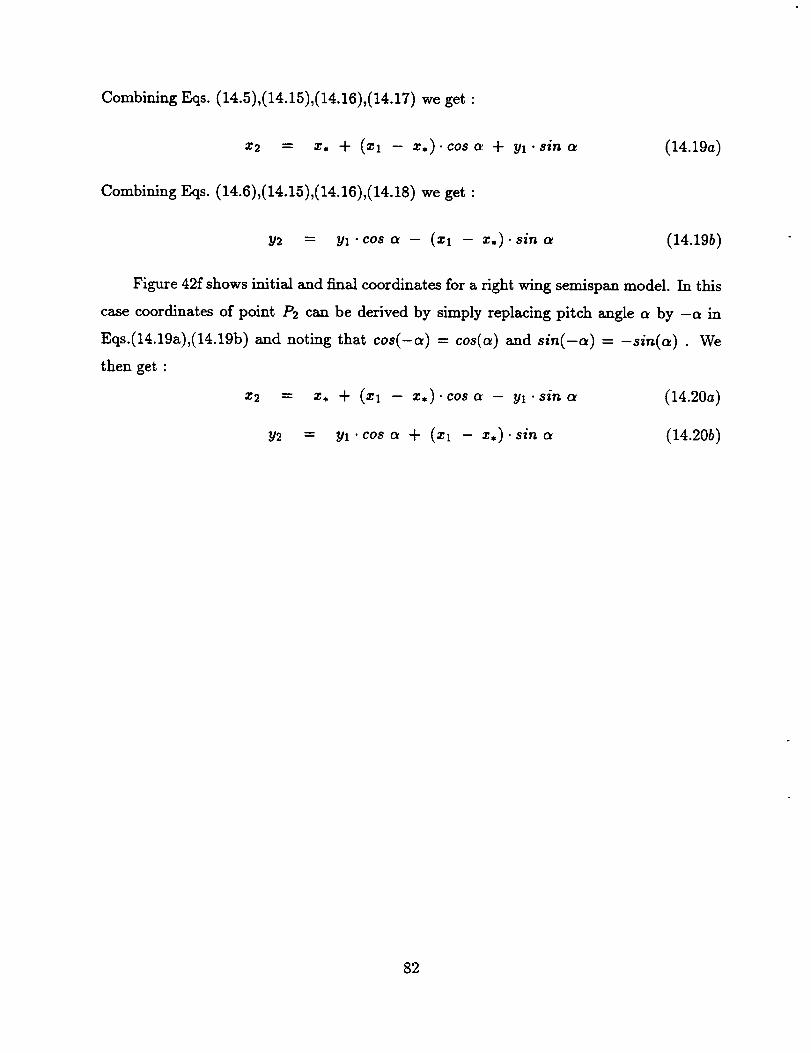
Combining Eqs. (14.5),(14.15),(14.16),(14.17)we get:
x2 = x, + (xl - z,).cos a + yl"sin a (14.19a)
Combining Eqs. (14.6),(14.15),(14.16),(14.18) we get:
Figure 42f shows initial and final coordinates for a right wing semispan model. In this
case coordinates of point P2 can be derived by simply replacing pitch angle a by -a in
Eqs.(14.19a),(14.19b) and noting that cos(-a) = cos(a) and sin(-a) = -sin(a) . We
then get :
x, Jr (Xl -- x,).cos a -- yl'sin a (14.20a)
= yl. cos a + (_ -- _,). sin a (14.20b)
82
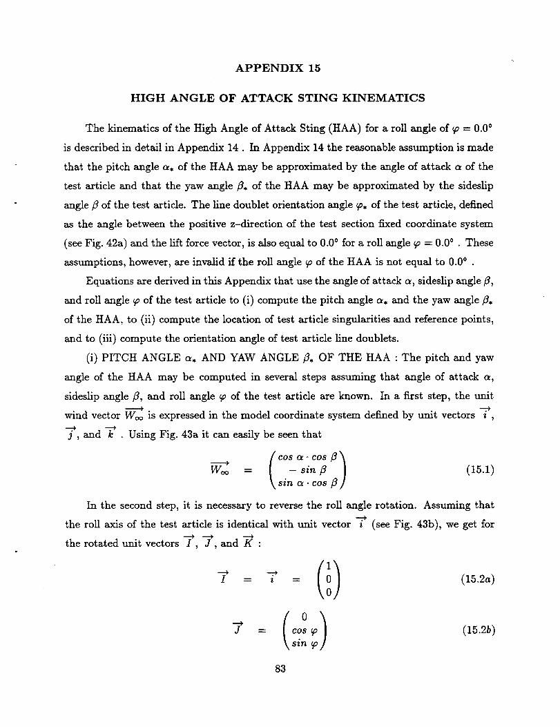
APPENDIX 15
HIGH ANGLE OF ATTACK STING KINEMATICS
The kinematics of the High Angle of Attack Sting (HAA) for a roll angle of to = 0.0 °
is described in detail in Appendix 14. In Appendix 14 the reasonable assumption is made
that the pitch angle a, of the HAA may be approximated by the angle of attack c_ of the
test article and that the yaw angle fl, of the HAA may be approximated by the sideslip
angle fl of the test article. The line doublet orientation angle _, of the test article, defined
as the angle between the positive z-direction of the test section fixed coordinate system
(see Fig. 42a) and the lift force vector, is also equal to 0.0 ° for a roll angle _ = 0.0 ° . These
assumptions, however, are invalid if the roll angle _ of the HAA is not equal to 0.0 ° .
Equations are derived in this Appendix that use the angle of attack c_, sideslip angle/_,
and roll angle _ of the test article to (i) compute the pitch angle a, and the yaw angle fl,
of the HAA, to (ii) compute the location of test article singularities and reference points,
and to (iii) compute the orientation angle of test article line doublets.
(i) PITCH ANGLE c_, AND YAW ANGLE fl, OF THE HAA : The pitch and yaw
angle of the HAA may be computed in several steps assuming that angle of attack a,
sideslip angle fl, and roll angle _ of the test article are known. In a first step, the unit
-----4 -:+wind vector Woo is expressed in the model coordinate system defined by unit vectors z ,
j , and k . Using Fig. 43a it can easily be seen that
cos ol o cos ,_)_t= | - (15.1)\ sin _. cos
In the second step, it is necessary to reverse the roll angle rotation. Assuming that
the roll axis of the test article is identical with unit vector z (see Fig. 43b), we get for
the rotated unit vectors I , J, and K :
I = z = 0 (15.2a)
0
(0)J = cos (15.2b)
\ sin
83
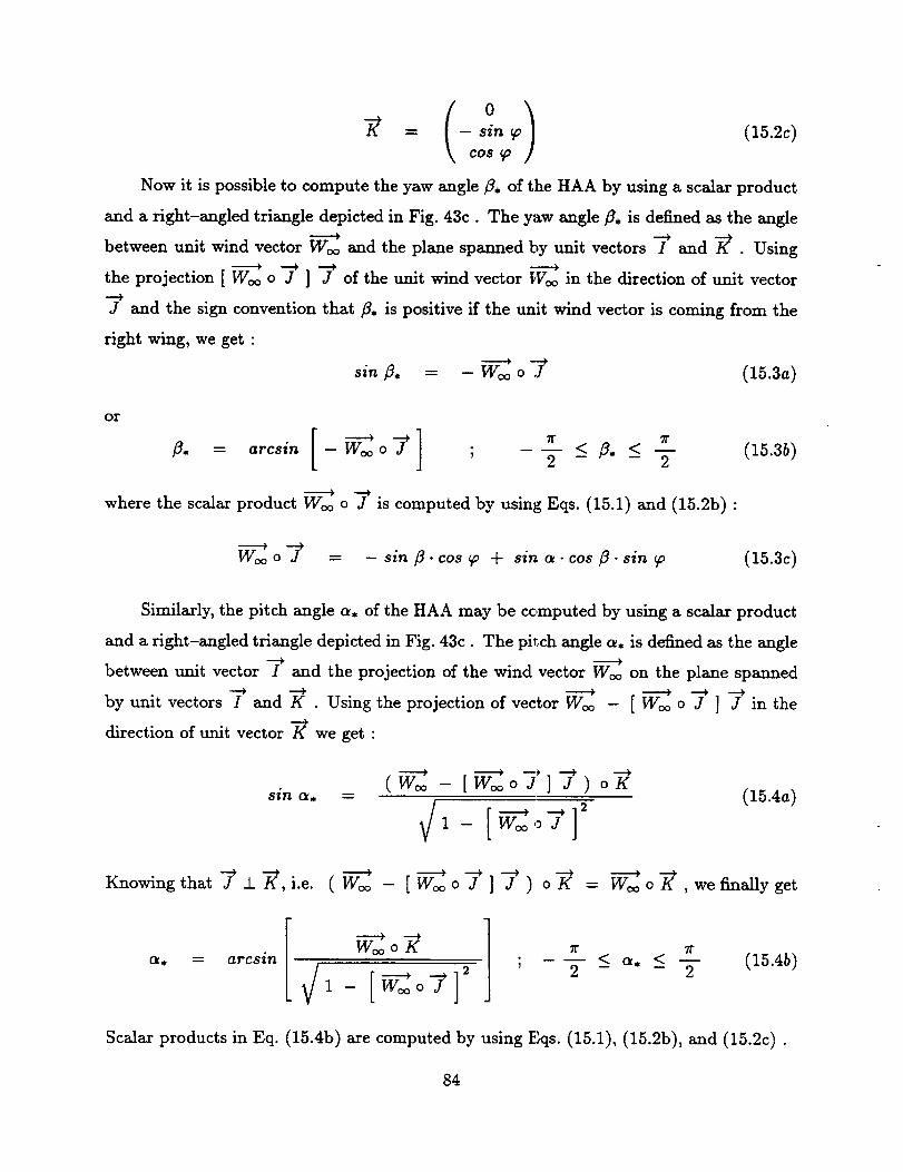
(0)= - sin _ (15.2c)
cos
Now it is possible to compute the yaw angle fl, of the HAA by using a scalar product
and a right-angled triangle depicted in Fig. 43c. The yaw angle fi, is defined as the angle
between unit wind vector Woo and the plane spanned by unit vectors -_ and _ . Using
the projection [ Woo o J ] J of the unit wind vector Woo in the direction of unit vector
J and the sign convention that fi, is positive if the unit wind vector is coming from the
right wing, we get :
-----} --4
sin fl, = - Woo o ,1 (15.3a)
or
] < /3. < (15.3b)fl, = arcsin -- Woo o-'f ; 2 - - "_
where the scalarproduct _ o 7 iscomputed by using Eqs. (15.1) and (15.2b) :
-----4 --.4
Woo o J = - sin fl. cos _ + sin a . cos fi. sin _ (15.3c)
Similarly, the pitch angle a, of the HAA may be computed by using a scalar product
and a right-angled triangle depicted in Fig. 43c. The pitch angle a. is defined as the angle......+ _.___+
between unit vector I and the projection of the wind vector Woo on the plane spanned
by unit vectors I and K . Using the projection of vector Woo - [ Woo o J ] J in the
direction of unit vector _ we get :
(woo - [Wooo j I-Y) oYsin c_, = (15.4a)
1 - Woo o J
-'_ "* ----* _ "* = Woo o K , we finally getKnowing that J 2_ K,i.e. (Woo - [Wooo J ]"#*) o]_ _ ---+
_. = arcsin7r 7?
; 2 < a_ < -_ (15.4b)
Scalar products in Eq. (15.4b) are computed by using Eqs. (15.1), (15.2b), and (15.2c) .
84
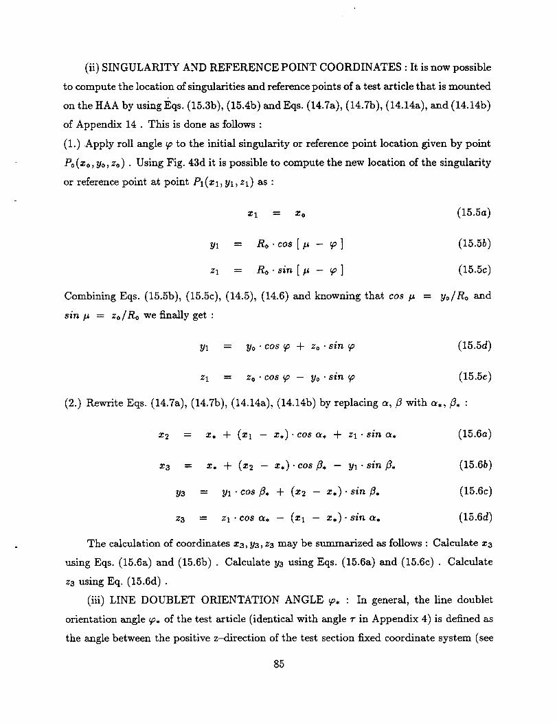
(ii) SINGULARITY AND REFERENCE POINT COORDINATES : It is now possible
to computethe location of singularities and referencepoints of a test article that is mounted
on the HAA by using Eqs.(15.35), (15.45) and Eqs. (14.7a), (14.75), (14.14a),and (14.145)
of Appendix 14 . This is done asfollows :
(1.) Apply roll angle_ to the initial singularity or referencepoint location given by point
P0 (xo, yo, z0) • Using Fig. 43d it is possible to compute the new location of the singularity
or reference point at point Pl(xl, yl, zl) as :
xl = z0 (15.5a)
vl = Ro . cOS [ l_ - _ ]
zl = Ro . sin [ _ - _ ]
Combining Eqs. (15.55), (15.5c), (14.5), (14.6) and knowning that cos I_
sin !_ = zo/ Ro we finally get :
(15.55)
(15.5c)
= yo/Ro and
yl = yo " cos _ + zo . sin (15.5d)
Zl = zo'cos _ - yo'sin _ (15.5e)
(2.) Rewrite Eqs. (14.7a), (14.75), (14.14a), (14.145) by replacing a, fl with c_,, fl, :
x2 = x, + (xl - ,).cos + zl.sin (15.6a)
x3 = z, + (z2 - x,).cos fl, - yl"sin fl, (15.6b)
ya = yl . cos _. + (a:2 - z.).sin _. (15.6c)
z3 = zl.cos _, - (_,_ - z,).sina, (15.6d)
The calculation of coordinates z3, y3, za may be summarized as follows : Calculate z3
using Eqs. (15.6a) and (15.6b) . Calculate y3 using Eqs. (15.6a) and (15.6c) . Calculate
z3 using Eq. (15.6d) .
(iii)LINE DOUBLET ORIENTATION ANGLE _, : In general, the line doublet
orientationangle _, of the testarticle(identicalwith angle r in Appendix 4) isdefined as
the angle between the positivez-directionof the testsection fixed coordinate system (see
85
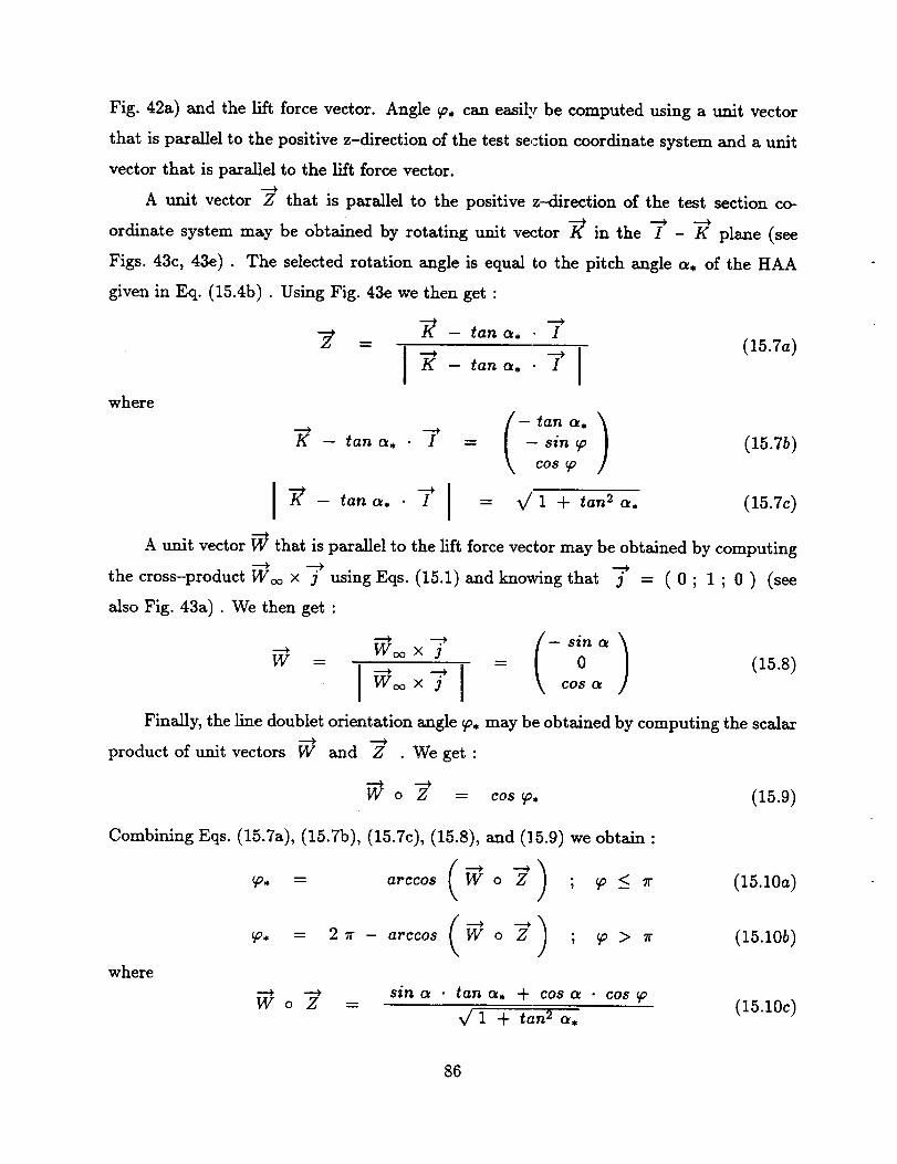
Fig. 42a) and the lift force vector. Angle _0, can easily be computed using a unit vector
that is parallel to the positive z-direction of the test section coordinate system and a unit
vector that is parallel to the lift force vector.
A unit vector Z that is parallel to the positive z-direction of the test section co-•----4 --_
ordinate system may be obtained by rotating unit vector K in the I - K plane (see
Figs. 43c, 43e) . The selected rotation angle is equal to the pitch angle c_, of the HAA
given in Eq. (15.4b) . Using Fig. 43e we then get :
where
K - tan _, • I
K - tan _, . I(15.7a)
K - tana, • I = - sin_o (15.7b)
cos _o
- tan _, I = V/ 1 + tan 2 _, (15.7c)
A unit vector W that is parallel to the lift force vector may be obtained by computing
the cross-product Woo × 3 using Eqs. (15.1) and knowing that -*" = (0; 1;0) (seealso Fig. 43a) . We then get :
_---* Woox 3W = = (15.8)
Woo x 3 \ cos a
Finally, the line doublet orientation angle _, may be obtained by computing the scalar----4 ---4
product of unit vectors W and Z We get :
o -_ = cos _, (15.9)
Combining Eqs. (15.7a), (15.7b), (15.7c), (15.8), and (1.5.9) we obtain:
where
_o, -- arccos W o Z ; _o < _" (15.10a)
_, = 2 _ - arccos o Z ; _o > r (15.10b)
---4
WoZ =sin _ • tan _, + cos _ • costa
_/1 + tan 2 _,(15.10c)
86
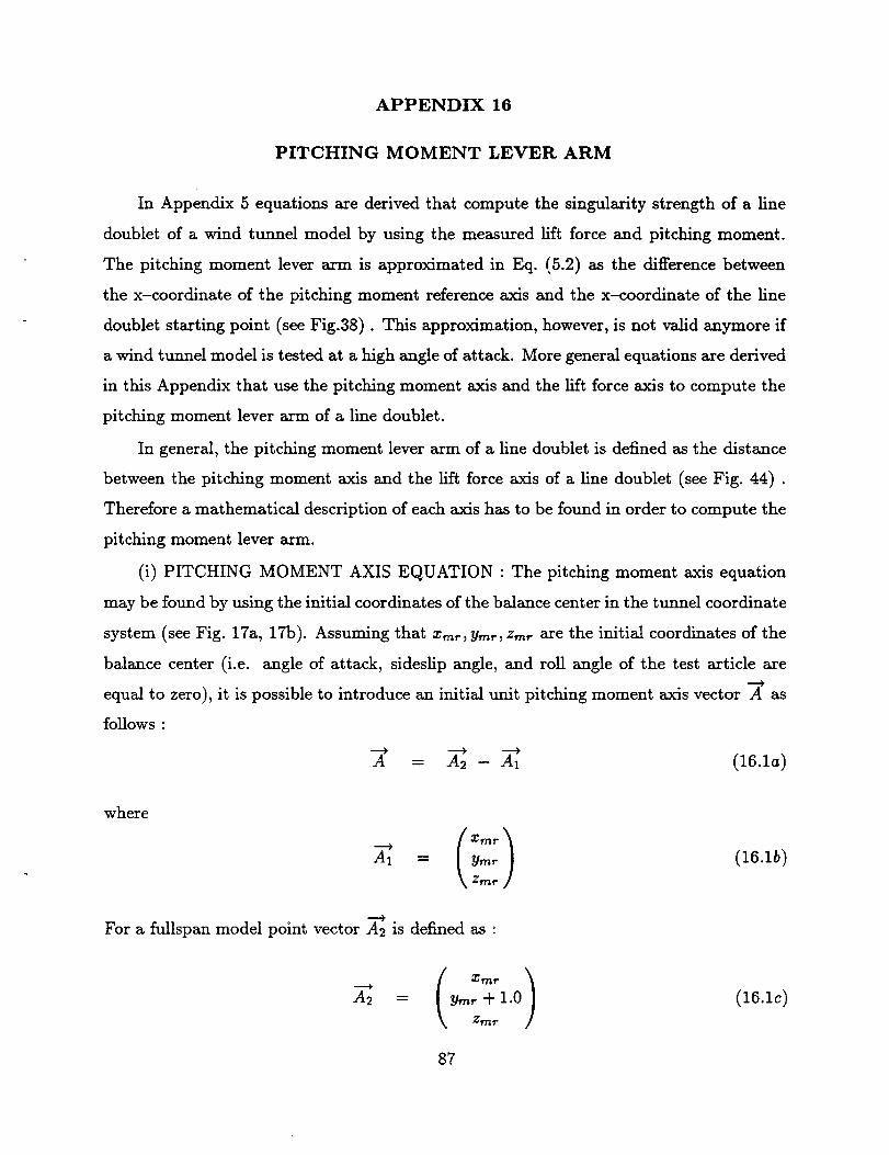
APPENDIX 16
PITCHING MOMENT LEVER ARM
In Appendix 5 equations are derived that compute the singularity strength of a line
doublet of a wind tunnel model by using the measured lift force and pitching moment.
The pitching moment lever arm is approximated in Eq. (.5.2) as the difference between
the x-coordinate of the pitching moment reference axis and the x-coordinate of the line
doublet starting point (see Fig.38). This approximation, however, is not valid anymore if
a wind tunnel model is tested at a high angle of attack. More general equations are derived
in this Appendix that use the pitching moment axis and the lift force axis to compute the
pitching moment lever arm of a line doublet.
In general, the pitching moment lever arm of a line doublet is defined as the distance
between the pitching moment axis and the lift force axis of a line doublet (see Fig. 44) .
Therefore a mathematical description of each axis has to be found in order to compute the
pitching moment lever arm.
(i) PITCHING MOMENT AXIS EQUATION : The pitching moment axis equation
may be found by using the initial coordinates of the balance center in the tunnel coordinate
system (see Fig. 17a, 17b). Assuming that X,nr, Yrn,', Zm,- are the initial coordinates of the
bMance center (i.e. angle of attack, sideslip angle, and roll angle of the test article are
equal to zero), it is possible to introduce an initial unit pitching moment axis vector -_ as
follows :
"_ = _22- _ (16.1a)
where
A1 = / 06.1b)\ z._r /
For a fullspan model point vector A2 is defined as :
2 = y,,_ + 1.0
Z vn r
87
.....4
For a left wing semispan model point vector A2 is defined as :
f Xrrlr /A2- |
\ z,_,. - 1.0
(16.1d)
For a right wing semispan model point vector A9 is defined as :
= l (16.1e)\ z_,- + 1.0
In the next step, equations describing the kinematics, i.e. the movement of the model
support system, have to be applied to the points described by vector _ and _ (see
Appendix 14 and 15). Point vector A1 moves to point vector -_ and point vector X22
moves to point vector C, . After points A1, _ are moved to their new location, it is
possible to describe the unit pitching moment axis vector D as :
.=.=4
D = C, - _ (16.2)
...=@
A point P on the pitching moment axis may now be described by using vectors
and an independent variable A :
----4 -----4 ---=4
P(_) = C + A. D (16.3)
(ii) LIFT FORCE AXIS EQUATION : The lift force axis equation of a line doublet
may be found by using the tunnel coordinates of the line doublet starting point in com-
bination with the line doublet orientation angle _, (see also Appendix 4 and 15) . After
the application of equations describing the support system kinematics, the line doublet
starting point has moved to a location described by point vector E . The line doublet
orientation is given by a unit lift vector F in the tunnel coordinate system :
F = sin _o, (16.4)
\ cos 9,
For a left wing semispan model 9, = rr/2, for a fight wing semispan model _, = -r/2 .
Similar to Eq. (16.3), a point _ on the lift force axis may be descibed by using vectors
E, F, and an independent variable/_ :
_( --'* .._,#) = E + ju. F (16.5)
88
(iii) PITCHING MOMENT LEVER ARM : The pitching moment lever arm of the
selectedline doublet is found by minimizing the squareof the distanceof points located on
eachaxis (seeFig. 44). The squareof the distanceof two selectedpoints may be computed
using a scalar product :
D2(A,/_) -- ['_(A) - _(/_)] o ['_(_) - _(/_)] (16.6)
Using Eqs. (16.3), (16.5) and applying the product rule to Eq. (16.6) we get :
a_= 2-[ "_(A) - -Q(/_) ] o _ (16.7a)
c9 D2(A,/_)= 2.[ _'(_) - _(,)] o [- _'] (16.7b)
The variables A,_i, and #,hi,, of the two closest points are found by setting Eqs. (16.7a),
(16.7b) to zero. We get :
(16.8a)
(16.8b)
Using Eqs. (16.3), (16.5), it is possible to write Eqs. (16.Sa), (16.Sb) as a 2 × 2 system of
linear equations :
In general, D _L F or D o F
closest points :
= 0 . Therefore, we get for A,'ni,_ and #mi,, of the two
Ami, ___ [ E - -_] o D (16.10a)-----4
DoD
[E - C]o r(16.10b)
-FoP
Finally, using Eq. (16.6), we get for the pitching moment lever arm :
D(A,_,/_,_,_) = _/[-_(A,_,,,) - _(/_,_,,_)] o [-P(A,n,,_) - -_(/_,n,,,)] (16.11)
89
The following two conditions may be used to determine the correct sign of the pitching
moment caused by a line doublet :
[_ × V]o[_(_..,.)-_(_,_,_)] > o _ "+"
[ D x _] o ['_(_,,_i,,) - Q(p_I,_)] < 0 ===_ "-"
These conditions ensure that the pitching moment is positive if the lift force axis of a
line doublet is upstream of the pitching moment axis (see also Eq.(5.2) and Fig. 38).
9O
APPENDIX 17
INCLINATION OF FORCE AND MOMENT VECTORS
Corrections to the lift, drag, rolling moment, and yawing moment coefficient are caused
by the wall interference induced inclination of corresponding force and moment vectors.
These four corrections may be estimated by describing the inclination of the force and
moment vectors using the induced mean angle of attack correction &] at the 1/4-chord
line of the wing (see also Ref. [181, p.17).
LIFT AND DRAG COEFFICIENT CORRECTION
The lift and drag coefficient correction caused by the inclination of the lift and drag
force may be estimated by using the resultant of the uncorrected lift and drag force vectors.
Using Fig. 45a we get for the resultant vector in the x-z coordinate system :
= D' + - L'
where Dr is the magnitude of the uncorrected drag force and L I is the magnitude of the
uncorrected lift force experienced by the wind tunnel model.
Unit vectors i , 3 in the free-stream direction and perpendicular to the free-stream
direction of the wind tunnel flow field have to be specified as they are used to define the
lift and drag force. These unit vectors are a function of the mean angle of attack correction
_ at the 1/4-chord of the wing. They may be written in the x-z coordinate system as :
-.-.':*._ ( cos _ ) (17.2a)z -- ksin a%
_ (17.2b)3 - \ cos at }
The mean angle of attack correction a"i may be computed by calculating the local
angle of attack correction at equally spaced reference points along the 1/4-chord line of
the wing. We then get :
N
1/4-chord line ==_ _i = .N (17.2c)Ej=I w(j)
91
where N is the number of reference points, w is the weighting factor of a reference point (a
function of the lift distribution of the wing), and cq is the local angle of attack correction
at a reference point. Now it is possible to compute the lift and drag force vectors as :
[ ]-- "- 3 (17.3a)
where
D - D , _o-_ --+"- = , (17.3b)
""* "-*" D' sin _ + L' cos o_L - Ro 3 = - • • (17.4a)
-*" D' L'D = -'_o , = "cosffi + .sinffi (17.4b)
The lift and drag coefficient correction may now be written as :
L - L'
ACL "-- CL -- C'L = qoo"-S (17.5a)
D - D'
ACD = CD -- c_9 = qoo" S (17.5b)
where qoo is the free-stream dynamic pressure and S is the reference area of the wind
tunnel model. A first order approximation of the free-stream dynamic pressure may be
obtained by using Eq. (1.15) in Appendix 1. Using the test section reference density,
velocity, and Mach number we get :
qoo = qrey [ 1 +
-- Prey 2
-- 2 U¢'eY
(2- MLy).
[1 + (2 - Me%y).(17.6a)
The mean blockage factor _ has to be computed as a weighted average of local blockage
factors e that are computed at a set of user selected reference points. We get :
= F_,_=I w(j). e(j)!,, (17.6b)Ej: o(j)
where N is the number of reference points, w is the weighting factor of a reference point,
and e is the local blockage factor at a reference point.
92
Important remark: The reference points used to compute the mean blockage factor
in Eq. (17.6b) axe not necessarily identical with the reference points used to compute the
mean angle of attack correction in Eq. (17.2c) I
Combining Eqs. (17.4a), (17.4b), (17.5a), and (17.5b) we get for the lift and drag
coefficient correction :
- D'.sina_ + L'.[cos_ - 1]ACL = -- (17.7a)
qo_ • S
D' . [ cos _ - 1] + L'. sinACD -- -- (17.7b)
qoo " S
Finally, corrections have to be added to the uncorrected lift and drag coefficients.
Then we get :
CL,c "- eL,uric "_- ACL (17.8a)
CD,c = CD,ur, c _L ACD (17.8b)
ROLLING AND YAWING MOMENT COEFFICIENT CORRECTION
The rolling and yawing moment coefficient correction caused by the inclination of
the rolling and yawing moment vector may be computed by using the resultant of the
uncorrected rolling and yawing moment vectors. Using Fig. 45b we get for the resultant
vector in the x-z coordinate system :
- r' = (:v.9)-- + _y,
where R' is the magnitude of the uncorrected rolling moment and Y' is the magnitude of
the uncorrected yawing moment experienced by the wind tunnel model.
Similar to Eqs. (17.3a) and (17.3b), it is possible to combine Eqs. (17.2a),(17.2b) with
Eq. (17.9) . Then, we get for the rolling and yawing moment vectors :
R -R "-_" "* -_"= , = o i , (17.10a)
where
R
[Y = -y = (17.10b)
-_ -_" R' ^ Y' ^ (17.11a)- o _ = ° cos oq -t- ° sin oq
93
--> - R' • Y'.Y = --_o 3 = sin _ + cos_i (17.11b)
The rolling moment and yawing moment coefficient correction may now be written as :
R-R'
A_ = ct - c_ = qoo.'S.b/2 (17.12a)
y _ yt' -- (17.12b)
A'O"j, = c,_ - c,, q_ • S. b/2
where qoo is the free-stream dynamic pressure, S is the reference area of the wind tunnel
model, and b is the wing span.
Combining Eqs. (17.11a), (17.lib), (17.12a), and (17.12b) we get for the rolling and
yawing moment coefficient correction :
R' . [ cos a'_ - 1] + Y' . sin _AW = _ (17.13a)
qoo" S. b/2
- R'.sin_ + Y'.[cos&_ - 1]A_-_ = _ (17.13b)
q_o. S. b/2
Finally, corrections have to be added to the uncorrected rolling and yawing moment
coefficients. Then we get :
ct,¢ = ct._nc + A'_ (17.14a)
c,_,_ = c,_,_,,¢ + A_--_ (17.14b)
94
APPENDIX 18
PITCHING MOMENT COEFFICIENT CORRECTION
Wall interferenceinduced angle of attack corrections are not constant in the test
section of a wind tunnel (see Fig. 24c). Therefore, it isnecessary to compute a pitching
moment coefficientcorrection that will account for the differencebetween the mean and
localangle of attack correctionin the spanwise and chordwise directionof the wing of the
testarticle.
In general,the corrected pitching moment coefficientCM, c of the complete testarticle
configuration may be written as :
CM,c --" CM,unc "Jr- ACM1 -Jr- ACM2 (18.1)
where CM,,_,_, is the uncorrected pitching moment coefficient, ACM: is the pitching moment
coefficient correction due to the difference between the mean and local angle of attack cor-
rection in the spanwise direction of the wing, and ACM2 is the pitching moment coefficient
correction due to wall interference induced streamline curvature in the chordwise direction
of the wing.
PITCHING MOMENT CORRECTION Acm: :
A pitching moment coefficient correction ACM: is due to the difference between the
mean mad local angle of attack correction in the spanwise direction of the wing. It may
Mso be interpreted as a correction resulting from the lateral shift of the spanwise center of
lift caused by wall interference effects.
The pitching moment coefficient correction ACM1 may be computed by using Eq. (3.58)
given in Ref. [10], which is essentially identical with Eq. (34) in Ref. [18] . Using the no-
tation introduced in the WICS Theory Guide we get :
ACM: = F . 180
2r 3 Y/ _d0.75,y) - W / '_,,,(Y) •
bI. J
F = (_r/2). A 2. (OcL/ao O. tan _o.2_ (18.2b)r.h + 2.(C%L/OO 0
where A is the aspect ratio of the wing, COCL/Cgo_is the lift curve slope in [1/rad], _o0.2s is
the sweep angle of the 1/4-chord line of the wing, ai(0.75, y) is the local angle of attack
95
correctionin [deg]along the 3/4-chord lineof the wing, _'_isthe angle of attack correction
in [deg]of the wing, w_ is a weighting factor derived from the liftdistribution(see also
Eq. (19.2c)in Appendix 19), y isthe spanwise coordinate, and b is the span of the wing.
In general,Simpson's Rule may be applied to Eq. (18.2a)ifACMI has to be determined
for a given wing. However, itisalsopossibleto simply discretizeEq. (18.2a) as long as the
localangle of attack correctionai(0.75,y) iscomputed at a largenumber of equally spaced
points along the 3/4-chord lineof the wing. Assuming that a totalnumber of N equally
spaced referencepoints were selected along the semispan of the wing (i.e.b/2 = N. Ay),
we get the approximation :
d _ T "Ay =: N
Using the abbreviation ww(y(j)) =- w_(j), Eq. (18.2a):may be discretized as:
N
180 b Nj=l
After rearranging terms we get :
F. r 1 N
b. 9o W- - • w.(j) y(j) (18.3 1j=.l
Sometimes it is necessary to distribute a total nualber of M equally spaced reference
points along the complete span of the wing (i.e. b = 1J • Ay). Then, using the absolute
value of y(j), Eq. (18.3c) becomes:
F • rr 1 M
ACM1 _ b 90 " _ _ [_,(0.75,j)--<] w,(j), lY(J)I (18.4)j--1
WICS uses Eq. (18.4) to determine the pitching moment coefficient correction ACM1
that is caused by the wall interference induced shift of the center of pressure of the wing.
PITCHING MOMENT CORRECTION ACM2 :
A pitching moment coefficient correction ACM_ due to the streamline curvature along
the chord of the wing has to be computed. Classical theory has shown that the magnitude
of this correction may be approximated by the camber of a two--dimensional circularly
cambered airfoil (see Ref. [18], p.17/18 and Ref. [28], p.91).
96
In general, the angle of attack correction _ is not constant along the chord of a wing.
This phenomena may be described as a wall interference induced streamline curvature that
is experienced by the wing. A constant streamline curvature may be found if we assume
a linear change of the angle of attack correction along the chord (see Fig. 46a) . Then, a
linear function 6cq may be defined as (see Fig. 46b) :
7r
_(_) = [ _(_) - _(0.50)] • _ [raa] (18.5)
The linear function 6(_i may be related to a two-dimensional circularly cambered
airfoil,[28], because its derivative with respect to _ is the streamline curvature. The pitching
moment coefficient about the 1/4-chord point of a circularly cambered airfoil is given in
Ref. [28] as:
c.(0.25) = _ _. _L (18.6)C
where f/c is the camber of the airfoil (see Fig. 47). The camber is related to the slope of
the circular arc at the 1/4 and 3/4-chord point. The slope is related to the upwash along
the chord. Then, using Fig. 47, we get :
1tan _ _ fl = -- •
2
1-- °
2
[ ( )o75][ _o,(o.25) - ,_,_(o.75)]
(18.7a)
Using triangle ABC in Fig. 47 we also know that
2 ftan_ _ Z = (18.7b)
C
Combining Eqs. (18.7a), (18.7b) we get for the camber as a function of the streamline
curvature :
f 1-_- = -_- • [ 6ai(0.25) - ecq(0.75)] (18.8)
Using Eq. (18.5) we also know :
7V
6ai(0.25) -- [cq(0.25) -- ai(0.50)] 180 [rad] (18.9a)
7V
6oL/(0.75) = [o_i(0.75) - cq(0.50) l 180 [rad] (18.9b)
97
Combining Eqs. (18.6), (18.8), (18.9a), (18.9b) we finally get for the pitching moment
coefficient of the two-dimensional circularly cambered airfoil as a function of the difference
between the angle of attack correction on the 1/4 and 3/4-chord point :
cu(0.25) = _ _ (18.10)-7- ' [_(0.75) - _,(0.25)] • 18--6
In the next step, it is necessary to integrate the pitching moment coefficient in the
spanwise direction of the wing. Assuming that the sweep angle to of the wing is 0.0 ° (see
Fig. 48), the local pitching moment coefficient of a wing segment of width dy about the
1/4-chord line may be written as
d P(y) (lS.11)cM(0.25,y) = qo¢ • c(y) d _(y)
where d P(y) is the infinitesimal pitching moment acting on the wing segment, qoo is the
free-stream dynamic pressure seen by the wing segment, c(y) is the local chord, and d S(y)
is the infinitesimal area of the wing segment. The infinitesimal area d S(y) of the wing
segment is a trapezoid and may therefore be expressed as :
d S(y) = c(y) d y (18.12)
Introducing the mean geometric chord as a function of the wing reference area S and the
wing span b we know :
S
= T (18.13)
In the next step we combine Eqs. (18.11), (18.12), divide both sides of the resulting equation
by the mean geometric chord -5 and the mean aerodynamic chord c', introduce Eq: (18.13)
on the right hand side of the equation, and rearrange terms. Then, we get :
cM(O.25, y) c2(Y) 1 d P(y)d._ -_- • dy = - (18.14)
qoo .d.S
The pitching moment coefficient correction ACM_ for 0.0 ° sweep angle may be obtained
by integrating both sides of Eq. (18.14) over the whole wing span :
[b/2 c2(y) d fo PACM_ = cM(O.25, y) y := d P(y) (18.15)J-b/2 d • "5 b q oo d • "S
98
The pitching moment coefficient of a swept wing may be approximated (see Ref. [29])
by using the product of the pitching moment coefficient of the unswept wing and the
cosine of an average sweep angle _. For a circular cambered airfoil the sweep angle at the
1/2-chord is selected. We get :
hcM,(_ # 0.0°) = cos Vo.50 Ac_(_ = 0.0°) (18.16)
Finally, combining Eqs. (18.10), (18.15), (18.16) we get for the pitching moment coefficient
correction ACM2 due to streamline curvature :
ACM2 ----" 7r. cos to0s0 ./b/2 7r c2(y) d y (18.17)4 J-bi_ [ _(0.75, v) - _(0.25, y) ]- 1--g6 e. _ b
The variable transformation # = 2y/b is introduced in an effort to compare Eq. (18.17)
with an equation reported in the literature. Assuming that the lift distribution is symmet-
ric, Eq. (18.17) may then be written as :
z . cos _o so [1 _ c2(_) dACM2
4 "Jo [a_(0.75,/_) - cq(0.25,#)]- 1-_ " d.e(18.18)
Equation (18.18) agrees with Eq. (35) in Ref. [18].
Assuming that local angle of attack corrections are computed on a total of N equally
spaced reference points along the 1/4-chord line of the wing and N equally spaced reference
points along the 3/4-chord line of the wing (i.e. b/2 = N. Ay), we get the approximation :
d_ _ A/_ = 2Ay = 1 (18.19)b N
Combining Eqs. (18.18), (18.19) we get an approximation of the pitching moment coeffi-
cient correction due to streamline curvature :
N [ ] c2(j) 1 (18.20a)_r. cos _0.50 _"
ACM2 _ 4 ._-_ ai(0.75,j)--a,(0.25,j) "1--8-0" c'- _ gj=l
Sometimes it is required to distribute a total number of M equally spaced reference
points along the 1/4- and 3/4-chord line of the complete span of the wing (i.e. b = M. Ay).
Then Eq. (18.20a) becomes :
_CM2
M
.cos 0 0 Z 1 c2(j) 1 (1820b)4 "1--8-6" d • _ Mj=l
99
Finally, introducing compressibility effects in Eq. (18.20b) (see Ref. [10], Eq. (3.59)),
we get :
where
M1
ACM2 _ G • M Z [c_/(0.75,j)- a/(0.25,j)] c2(j) (18.21a)j--1
G = 7r. cos _oo.so . _r 1 (18.21b)4. V/1 - M 2 • cos2_oo.5o 180 d
Equation (18.21a) and (18.21b) are used by WICS to determine a pitching moment
correction due to streamline curvature.
CALCULATION OF PITCHING MOMENT COEFFICIENT CORRECTIONS :
WICS uses Eq. (18.4) and Eqs. (18.21a,b) to compute pitching moment coeitlcient
corrections due to the difference between the mean and local wall interference corrections
in the spanwise and chordwise direction of the wing of a wind tunnel model. Input variables
required for the application of these equations axe classified as follows : (1) variables that
depend on the geometry of the test article (A, c, c', 5, too.25, to0.50), (2) variables that
depend on the lift of the wing (w,,(j), OCL/Oa ), m_d (3) variables that are a result
of the calculation of mean and local wall interference corrections (_'_, cq(j); ai(0.25,j),
c_(0.75, j)). For best results it is recommended to determine the lift curve slope OCL/(9o_
by using the experimental cL -- o_ curve.
100
APPENDIX 19
ROLLING MOMENT COEFFICIENT CORRECTION
An additional rollingmoment coefficientcorrection Act has to be found whenever
wall interferenceeffectsare the resultof a non-synunetric liftdistributionon the wing. A
non-symmetric liftdistributionmay be caused by deflectedailerons or non-zero sideslip
angle of the wind tunnel model.
In general, the corrected rollingmoment coefficientct,cof the complete test article
configuration may be written as :
ct,¢ = cz,,.,,-,¢ + Act (19.1)
where ct,,.,,.,_ is the uncorrected rolling moment coefficient and Act is the rolling moment
coefficient correction due to wall interference effects.
The calculation of the rolling moment coefficient correction is done in three steps. At
first, it is necessary to find a reasonable non-symmetric lift distribution and line doublet
representation of the wing that satisfies the measured lift force, pitching moment, and
rolling moment of the test article. Then, angle of attack corrections along the 3/4-chord
of the wing are computed using the non-symmetric line doublet representation of the wing
and the wall signature method. Finally, the rolling moment coefficient correction Act is
determined by integrating the angle of attack correction distribution.
LIFT DISTRIBUTION AND LINE DOUBLET REPRESENTATION :
The calculation of a rolling moment coefficient correction is only possible if a non-
symmetric lift distribution of the wing is found that matches the measured lift force,
pitching moment, and rolling moment of the test article. This lift distribution may be
obtained in two steps by using results presented in Appendix 5.
At first, a symmetric lift distribution of the wing is assumed. The corresponding
circulation F* of the wing is written as (see Appendix 5 for more detail) :
r*(y) = r_ w_(y) (19.2a)
where rw is only a function of the lift force and pitching moment measurement on the test
article and w_ (y) is the weighting factor of the selected symmetric lift distribution. The
101
weighting factor w,_ (y) has to fulfill the condition :
jff/2 w,_(y) d y = b (19.2b)b/2
The weighting factor ww (y) of an elliptic lift distribution (b - wing span) is given as :
The total lift caused by the symmetric lift distribution may be computed by integrating
the circulation along the wing span. Using Eqs. (19.2a), (19.2b) we get :
bl_L(r') = poo .uoo. r*(y) d y = poo -uoo. F,_. b (19.3a)J-b�2
Similarly, we get for the total pitching moment caused by the symmetric lift distribu-
tion :
b12P(r*) = pop-up. A_(y) r'(y) dJ -b/2
b/2= poo .uoo.r_. A_.(y) • w,_(y) d y,_-b12
where Ax(y) is the pitching moment arm.
(19.3b)
In a second step, a weighting factor Aw is applied to the symmetric lift distribution
such that the total rolling moment caused by the resulting non-symmetric lift distribution
equals the measured rolling moment R. The weighting factor Aw must be introduced such
that the total lift force and pitching moment of the nort-symmetric lift distribution equals
the lift force and pitching moment of the symmetric lift distribution. This weighting factor
Aw may be defined as follows (see Figure 49) :
r"(_) = r'(_) [1 + Aw ] ; y < 0 (19.4a)
r**(y) = r*(y) ; y = 0
r*'(y) = r'(_) [1 - _w] ; _ > 0
where F** is the circulation of the non-symmetric lift distribution of the wing.
(19.4b)
(19.4c)
102
Combining Eqs. (19.2a), (19.4a), (19.4b), and (19.4c) it is possible to express the
non-symmetric lift distribution asa function of the symmetric lift distribution. Similar to
Eq. (19.2a), we get for the circulation of the non-symmetric lift distribution :
r'*(y) = r_ • D"g'_(y) (19.5a)
where
W'j(y) = w_,(y) ; y = 0 (19.5c)
W-_(y) = w,,,(y) [1 - Aw ] ; y > 0 (19.5d)
In the next step it is necessary to show that the lift and pitching moment caused by the
non-symmetric lift distribution F** is identical with values obtained from the symmetric
lift distribution F*. Integrating the circulation F** of the non-symmetric lift distribution
along the wing span and introducing Eqs. (19.5a) we get :
bl2L(r*') = poo-uoo. F'*(y) d yJ-_/2 (19.6a)
bl2= poo • uoo. r_ • _'7_(y) d yJ-hi2
Using Eqs. (19.2b),(19.5b),(19.5c),(19.5d) and knowing that w_(y) is symmetric to y = 0
w_(_) • [ 1 - A_ ] d (19.6b)
b/2 ]_(y) d y - w_(y) d yJ0
we get :
b/2 _--J(y) d yb/2
lj ¢"- _-_(y) d y q- W-_(y) d yb/2 Jo
fj= _,,,(_) o [ i + Aw ] d _, +_/2 .,o
= w,,,(y) d y + Aw •J-b�2 b/2
= b
Thus, combining Eqs. (19.6a), (19.6b) and comparing the result with Eq. (19.3a) we con-
clude that :
L(F**) = poo .uoo.r_. b = L(F*) (19.6c)
103
Similarly, we get for the pitching moment of the non-symmetric lift distribution :
b/2e(r") = poo-_oo- _(_) • r"(y) d yJ-b/2
hi2= poo "uoo" r=. _z(y)._-;_(y) d yJ-b/2
(19.7a)
Using Eqs. (19.5b),(19.5c),(19.5d) and knowing that Az(y). w,_(y) is symmetric to y -- 0
we get :
A_:(y) . _--¢_(y)d y +
[1 - Aw] dy
b/2w,_(y)d _,- /',x(y)JO
(19.7b)
Thus, combining Eqs. (19.7a), (19.7b) and comparing the result with Eq. (19.3b) we con-
clude that :
b/2P(r**) = poo.uoo-r=. Az(y) • w=(y) dy = P(r*) (19.7c),_-b/2
In Eqs. (19.6c) and (19.7c) it was shown that the introduction of the weighting factor
Aw does not change the lift force and pitching moment. It remains to determine Aw as a
function of the rolling moment measurement. This may be done as follows :
The calculation of the angle of attack correction based on the wall signature method
requires that the non-symmetric lift distribution of the wing has to be translated to a
corresponding non-symmetric line doublet representation of the wing. We assume that a
104
total number of nw equally spaced line doublets are selected along the 1/4-chord line of
the wing. Then, the strength o'U(y(i)) of a line doublet at the spanwise location y(i) is
defined as (see also Eq. (5.4a) in Appendix 5) :
_,(y(i)) = A_ r_ • _-_(u(i)) (19.8_)
where W"_(y(i)) is given by Eqs. (19.5b), (19.5c), (19.5d) and
bAs_ = (19.Sb)
nw
b [ 1] 1o8c,y(i) = 2 + As_o i-- -_-
The total rolling moment caused by the non-symmetric line doublet representation of
the wing may now be written as :
-R = E L,_(i) . y(i) (19.9a)i=1
where L,_(i) is the lift force caused by a single line doublet at the spanwise station y(i).
Equation (19.9a) may also be written as the sum of the contributions from the left and
right wing. For an even number nt0 of line doublets we then get :
-R = E L,_(i) y(i) + E L,,,(i) . y(i) (19.9b)
i=1 i--n_/2+l
Applying the Kutta/Joukowski formula to the wing span increment As,_, introducing
Eq. (19.5a), and using the abbreviations F*'(y(i)) -- F'*(i) and _-'_(y(i)) - W'_(i) we get:
L_,(i) = p_ .u_. Asw. r**(i) = p_ .u_. As_.F,_._g_(i) (19.10)
Combining Eqs. (19.5b), (19.5c), (19.5d), (19.9b) and (19.10) we get :
-R
poo • uoo • Asw • Fw= [I+A_].
n.12
Z w_(i). _(0i=1
+[l-Awl._"b tl;
Ei=n,_/2+l
ww(i) . y(i)
(19.11)
105
The weighting factor w,_(i) of the symmetric lift distribution is symmetric to the root of
the wing (y = 0). Therefore, we know :
v(i) = - (19.12)i=rtw[2+l i=it
Combining Eqs. (19.11) and (19.12) we get:
-R
poo • uoo • Asw • I'w= 2 • Aw •
n./2
E Ww(i). y(i) (19.13)i=1
After rearranging terms in Eq. (19.13) we get for the weighting factor Aw :
(19.14a)V'n,,/22 • poo "uoo" Asw. r_o z-..,i=l ww(i) y(i)
where the number nw of line doublets of the wing is even. Assuming that the number nw
of line doublets of the wing is odd, we get :
Aw = -R (19.14b)
2 • j0oo "t too" Asw, I'_w £-_i=1 ww(i ) y(i)
Finally, non-symmetric line doublet strength values trw*(y(i)) that satisfy the mea-
sured lift, pitching moment, and rolling moment may be determined by using Eqs. (19.5b),
(19.5c), (19.5d), (19.8a), (19.14a) and (19.14b).
The angle of attack correction tr_ along the 3/4-chord line of the wing may now be
computed by applying the wall signature method as the line doublet representation of the
wing is known (for more detail see Chapter 2) .
ROLLING MOMENT COEFFICIENT CORRECTION :
It is now possible to compute a rolling moment coefficient correction due to wind
tunnel wall interference effects as the angle of attack correction along the 3/4-chord line of
the wing is known. Figure 50 shows the angle of attack correction distribution ai(0.75, y)
as a function of the spanwise coordinate y of the wirg. Using Fig. 50, we get for the
infinitesimal rolling moment of a wing span increment d y :
dcL(y) . _(0.75, y) • q:_ d S (19.15)dR = (-1) Y " dcr
106
The infinitesimal area d S of the wing span element may be written as :
d S = c(y) •d Y (19.16)
where c(y) is the local chord of the wing. Combining Eqs. (19.15) and (19.16) and integrat-
ing the corresponding equation in the spanwise direction, we get for the rolling moment
due to wall interference effects :
[_,/2 d cL(y) . 0_i(0.75,y) • c(y) •d y (19.17)A R = qoo a-b�2 (-y) dot
The rolling moment coefficient correction Act has to be added to the uncorrected
rolling moment coefficient (see Eq. (19.1)). Therefore we get:
AR
Ac, -- (-1) • qo_ "S. b/2 (19.18)
Finally, combining Eqs. (19.17), (19.18), the rolling moment coefficient correction is ob-
tained as :
2 [b/2 d cL(y) . ai(0.75, y) c(y) . d y (19.19a)Act = "S • b a-b/2 y " d o_
In general, Simpson's Rule may be applied to Eq. (19.19a) if Act has to be determined
for a given wing. However, it is also possible to simply discretize Eq. (19.19a) as long as
the local angle of attack correction cq is computed at a large number of equally spaced
points along the 3/4-chord line of the wing. Assuming that a total number of M equally
spaced reference points were selected along the complete span of the wing (i.e. b = M. Ay
and dy ,_ Ay = b/M), we get the approximation :
Ac, _ -_ "M2 1 EM Y(J) d d o_cL(j) . ai(0.75,j) c(j) (19.19b)j=l
where
-b b [ 1
Y(J) = 2 + -M" [ j 2 (19.19c)
The application of Eq. (19.19b) requires an estimate of the local lift curve slope
dcL(j)/do_ at the spanwise station of a reference point. This estimate may be obtained by
107
using the Kutta/Joukowski formula. For an infinitesimal wing span increment dy we get
for the lift dL using the non-symmetric lift distribution :
d L = poo uoo r"(y) • d y (19.20a)
The local lift coefficient is defined as :
dL
cz(y) = poo/2" u L c(y) . d y (19.20b)
Combining Eqs. (19.20a), (19.20b) we then get :
eL(y) = 2 r'*(y) (19.21)uoo c(_)
Combining Eq. (19.5a) with Eq. (19.21) and differentiating both sides of the resulting
equation with respect to angle of attack c_ we get :
d CL(y) 2 • _ww(Y) d r w
d a uoo e(y) d a (19.22)
Introducing the abbreviation y(j) - j, we get at the di,'_crete spanwise position j :
d eL(j) 2 _-'_(j) d Fw
d _ _ • _(j) d (19.23)
Assuming that the-total lift of the model is charged to the wing, we get from Eq. (19.6c) :
L poo u,_ F_ b cL poo 2. -- . Uoo2 (19.24)
Differentiating both sides of Eq. (19.21) with respect to the angle of attack a and
rearranging terms we get :
d F,_ _ uoo • S d cL-- (19.25)dot 2 • b da
Thus, combining Eqs. (19.23), (19.25) we get the following approximation of the local
lift curve slope :
d _L(j) _-_(j) _ d _L"_ (1926)
d a c(j) b d oL
108
Finally, combining Eqs. (19.19b), (19.26) we get for the rolling moment coefficient
correction due to wall interference effects :
2 dcL 1 M
Act ,_, b do_ U E Y(J) " "w-'_(J) _i(0.75,j) (19.27)j=l
where dcL/da is the lift curve slope of the wing in [1/deg], b is the wing span, M is the
number of reference points in the spanwise direction of the wing, y(j) is the spanwise
coordinate of reference point "j", _'_-_(j) is the weighting factor of the non-symmetric
lift distribution of the wing at reference point "j", and ai(0.75,j) is the angle of attack
correction at reference point "j" in [deg]. An interesting interpretation of Eq. (19.27)
is possible if we introduce the absolute value of y(j) and assume that y(j) # O. Then
Eq. (19.27) becomes :
Acl "" M E Y(J) ly(J)l _j(9). dcL . _d0.75,j) (19.28)"" lY(J)[ b / 2 do_j--1
Equation (19.28) may be interpreted as the arithmetic mean value of weighted rolling
moment coefficient contributions along the 3/4-chord of the wing where
y(J)I (J)l
---- sign of the local rolling moment correction
ly(J)l
b� 2-- dimensionless rolling moment arm
dcL
_-_-w(j)" dc_ .ai(O.75,j) = local lift coefficient
Equation (19.27) is used by WICS to determine a rolling moment coefficient correction
due to wind tunnel wall interference effects.
109
110
APPENDIX 20
SCALE FACTOR LAW
The minimum of the blockage factor of a wind tunnel model tested in a clean configu-
ration (i.e. flaps, slats not extended and no landing gear) is more or less identical with the
solid volume blockage contribution. This approximation is valid if such a model is tested
in the vicinity of 0.0 ° angle of attack where solid volume blockage effects are significantly
larger that corresponding separation wake blockage effects.
Solid volume blockage effects are a function of the volume displacement of the wind
tunnel model. The solid volume blockage factor is proportional to the volume of the test
article. Therefore, it is possible to develop a scale factor law, that relates the length scale
of two models of different size but identical geometry to the observed minimum of the solid
volume blockage. The scale factor law may be written as :
¢2 (20.1)
where e,n_ is the minimum of the blockage factor as a function of the length scale of the
model, ¢1 is the length scale of the first model, and ¢2 is the length scale of the second
model.
The following example shows how this scale factor law may be applied to a test of
two different sized Boeing 7J7 semispan models (see Chapter 3.3 for more detail). Both
semispan models had identical geometry. The first model was a 8 % scale model, the second
model was a 14 % scale model. Both models were tested in a cruise configuration. From
Fig. 23a we estimate that the minimum of the blockage factor computed by WICS (wall
signature method) and the two-variable method for the 8 % scale model is approximately
0.0030 . Now it is possible to predict the solid volume blockage factor of the 14 _ model
by applying the scale factor law. Using the blockage factor minimum of the 8 % model
and the cube of the scale factor ratio we get the prediction :
! 8% ] = 0.0030- 5.36 -- 0.0160 (20.9-)
Comparing the predicted solid volume blockage factor, i.e. 0.0160, with the estimate
of the solid volume blockage from Fig. 23b, i.e. 0.0155, we see that both values agree
111
fairly well. Therefore, it can be concluded that the wall pressure measurements used by
WICS to determine blockage corrections and the corresponding description of the solid
volume blockage effect by a source/sink pair is sufficiently accurate. The scale factor
law also provides an additional absolute magnitude check of blockage corrections that are
computed by using wall pressure measurements.
112

FIGURES
113
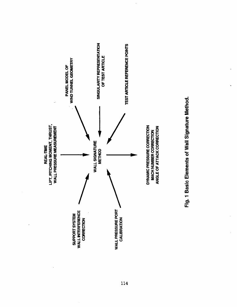
!oi_'i I°
m
! °o_,
/
114
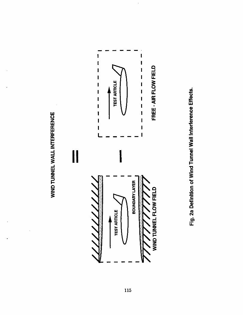
.JRI
Z
I-
;[m
0
,_" "E
115
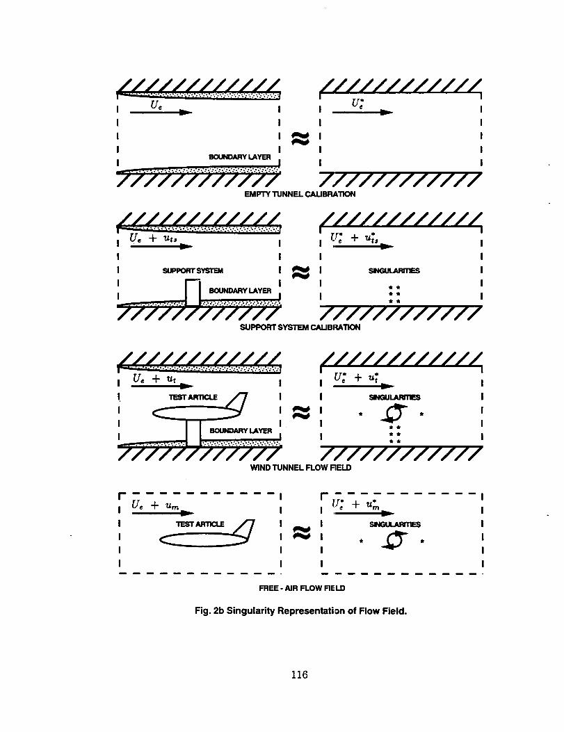
I Uc _ Iv
I I
I I
I IBOUNI_IUqYI.AYI_I
I .....................I
////////////
v
////////////EMPTY TUNNEL CALIBRATION
////////////.I I',. -- i I
I Ue -i- uts._ I I ue + _ts.__ II I I _ I
I SUPPORTSYSTEM I _ I SI_GULARmES III r-i .,...,..,,, .,, i I ** I
i :: i////////////
SUPPORT SYSTEM CALIBRATION
////////////I... . I
I Ue + ut_ I I U; + ut I
' _'_'_/'7 ' ' "_" '
I I I "_'-. I
////////////WIND TUNNEL FLOW FIELD
! I f II Ue + urn._ I i {7; + u_ I
I I _ I , . II I I I
I I I Im m _ _ m m m _ m a _ • m m _ m m m _ m m m _ _ -
FREE - AIR FLOW FIELD
Fig. 2b Singularity Representation of Flow Field.
116
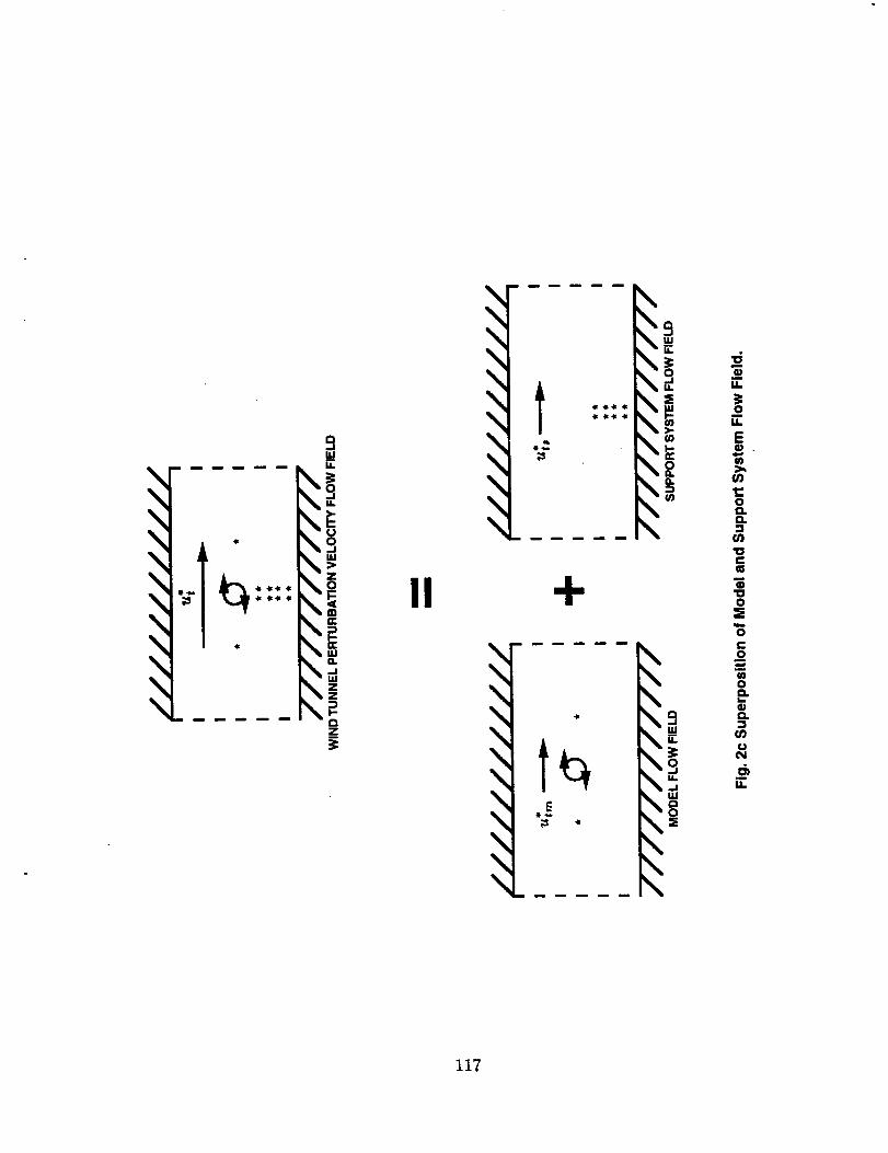
-dI/.
_oL
E0 .
0D.O.
if)
"0(-
m
o
0Z
0c-
Om
t00
G
u
117
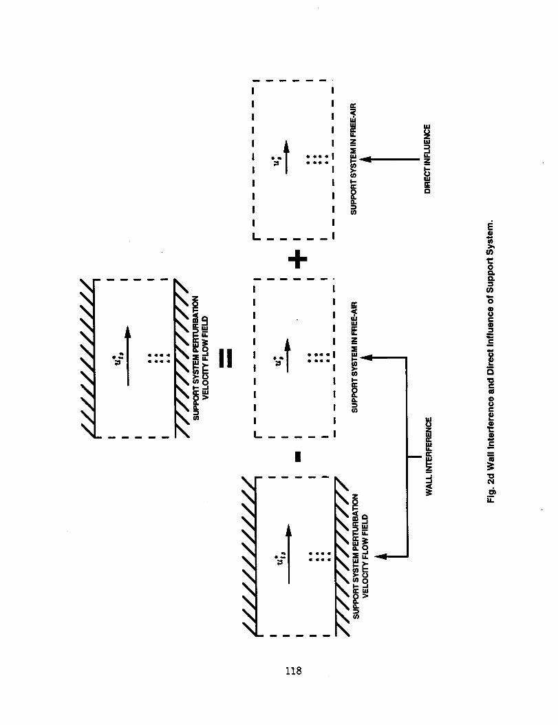
I I
' '!I I
I .. -o.°I
n n _,! I
L. ...... I
--: ----*--i! ,,-
T i ' 'II , o_ , ,
! !
I_ ....... I,P
' -Ii!0
_,i°
o
0Q.D.
U)
0
0uCo_=m
u
o
uC0
0
0
a
U.
118
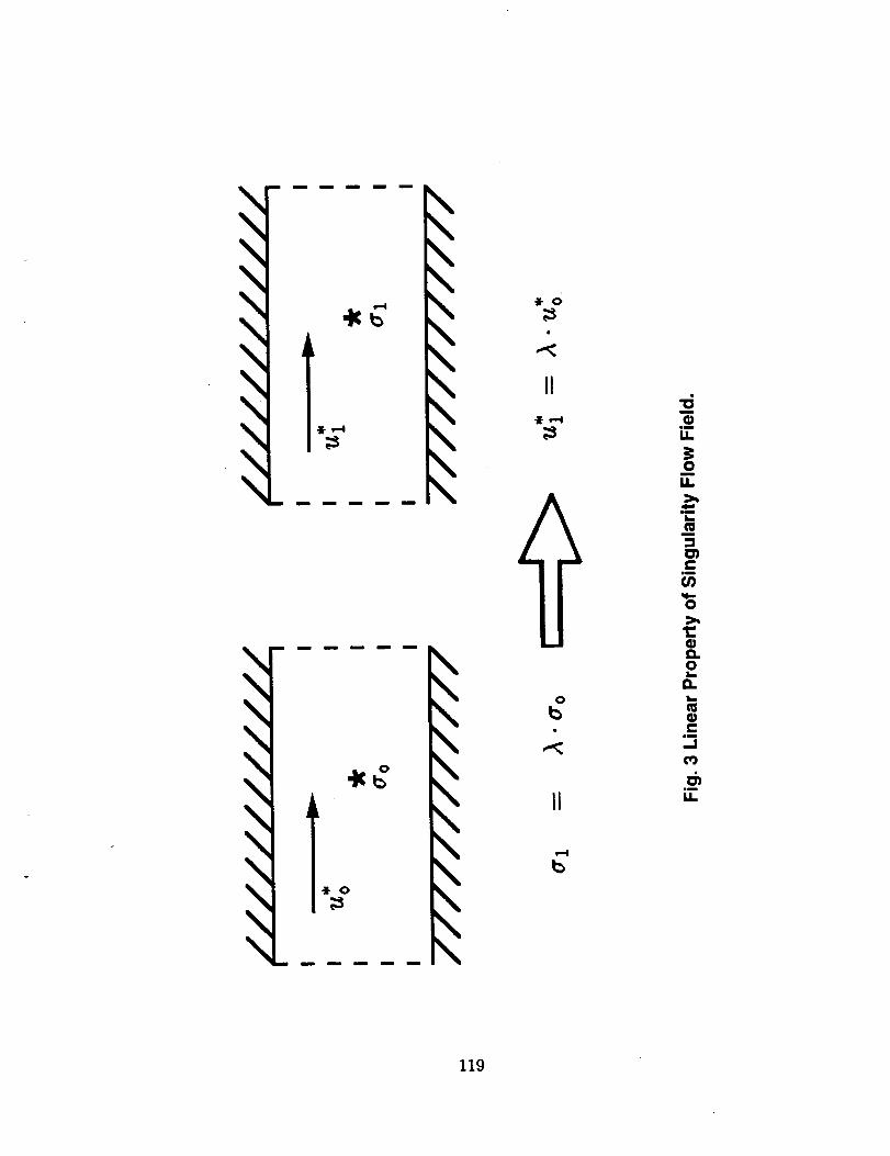
\\\\\\\\\\\\
\\\\\\\\\\\\
0
m u n m B
[,,,,\ _°\
\ II
\\\\\[,,,,[',,,l",,
0
!
II
m
I.I.
0m
1,1.,
ll
m
e"ml
0
0
13.
e.,tm
..I
ii
I.I.
119
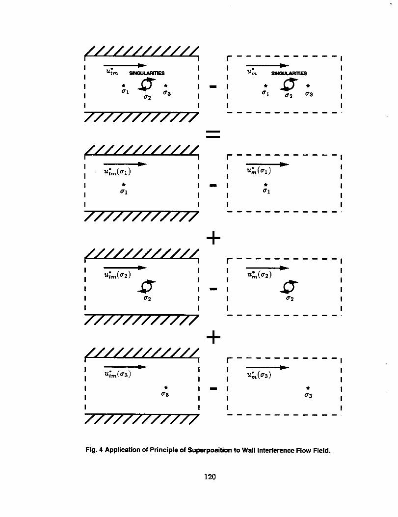
////////////! ! r
i i i
I * ._ * I -- I * ._ *°'I 0"3 o"1 o'3I _r_ I I or2
I I I
////////////
l
I
I
I
I
i
m
////////////I I I--"--"
I ut'_(_1) I I
I * I " I *
I crl I I o'I
I I I
////////////
r
////////////I I
+
p i i n m m m u m i m m I
I I I I
l _ I -- I _ l
I _ I I _2 I
I I I I
+////////////
////////////i i r I
i ,,;._(_3) i i . -- iI I I urn(0"3) I
I * I l I * II or3 I I o'3 I
I I I I
////////////
Fig. 4 Application of Principle of Superposition to Wall Interference Flow Field.
120
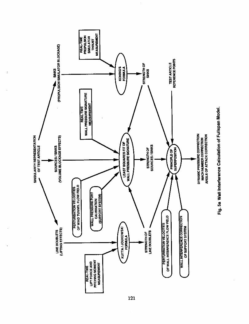
121
{D
0
e_
m
U.
0e._o
_u
00o
i-
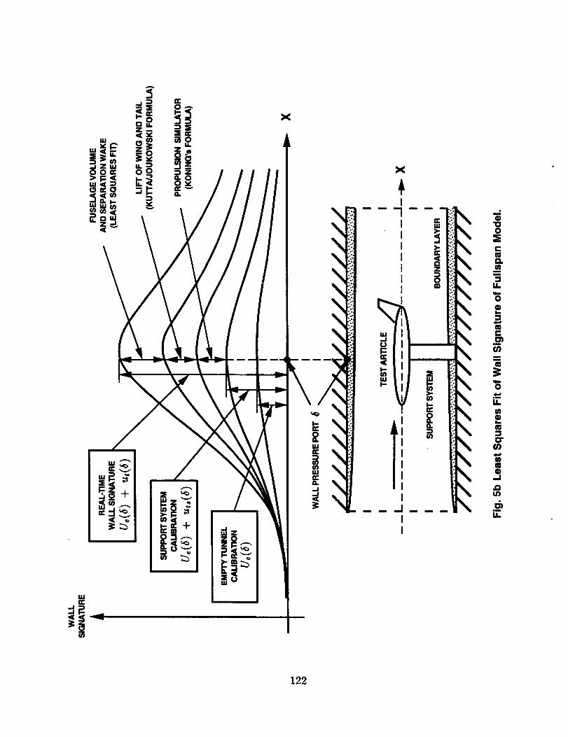
+
tM
Z
122
i
1 >':"_ ti:ik\
I _ .:...
_-' iii
_ I i-?
I
'U0
e-
a,w
II
0
C
¢/I
0
Im
crl
,.I
m
i1
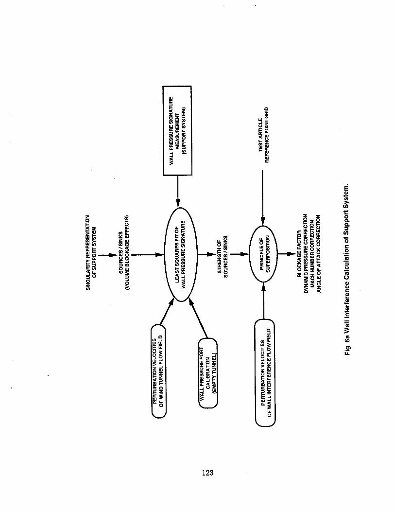
kl,I
m
ffl
0
n
b0
e-oo_
o
c
e-
°_
123
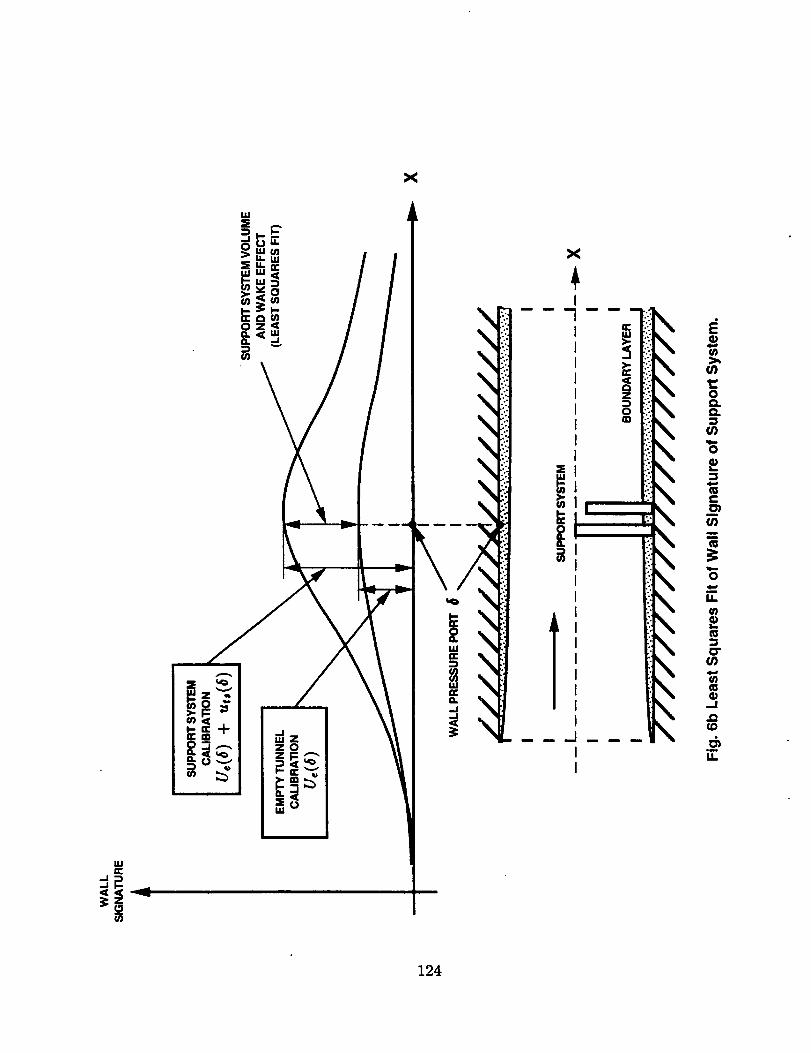
nl
)<
\
124
i
, _ l_:!k\i oi:
,-r
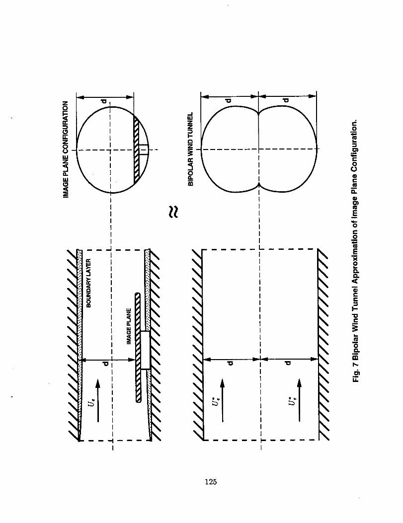
i - !-
k.
i i m
\\\\\
\
0if
¢gL--
Im
¢-00
G
m
O.
Ei
@
¢-0m
mEX@1,._
e_n.%n
CC
F-
¢-m
L_
m
0e_
mt_
omU.
125
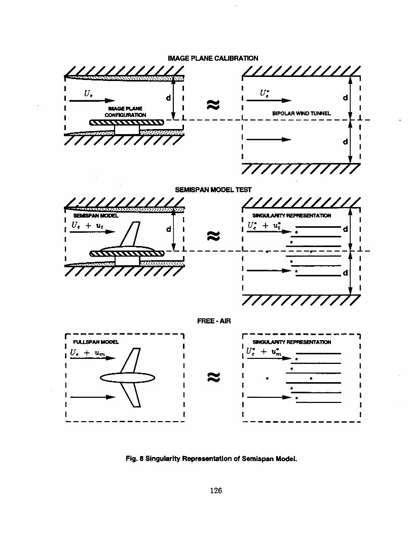
IMAGE PLANE CAUBRATION
i Ue d i
///////////
u:v
BIPOLAR WIND TUNNEL
d
/I
I
I
I
.I.
I
d II
SEMISPAN MODEL TEST
///////////I
_A110NIiu: +_;_
v *
I ,
i /r- if
I ,I b..._
I
d
d
/I
I
I
I
.L
I
I
I
/7 0iiI v I
lmliilim_mmiim_
_AN MODELI I
i U_+ _ i
Urn
I I
I I
I I
I I
I I
I I
FREE - AIR
ilWmilmmiiimmm_
SINGULAJ:h'rYREPRESIDI_'rATIONI II U: +_:'.- I
r *
I , I
I , , I
I , I
I .__ . II I
I I
Fig. 8 Singularity Representation of Semispan Model.
126
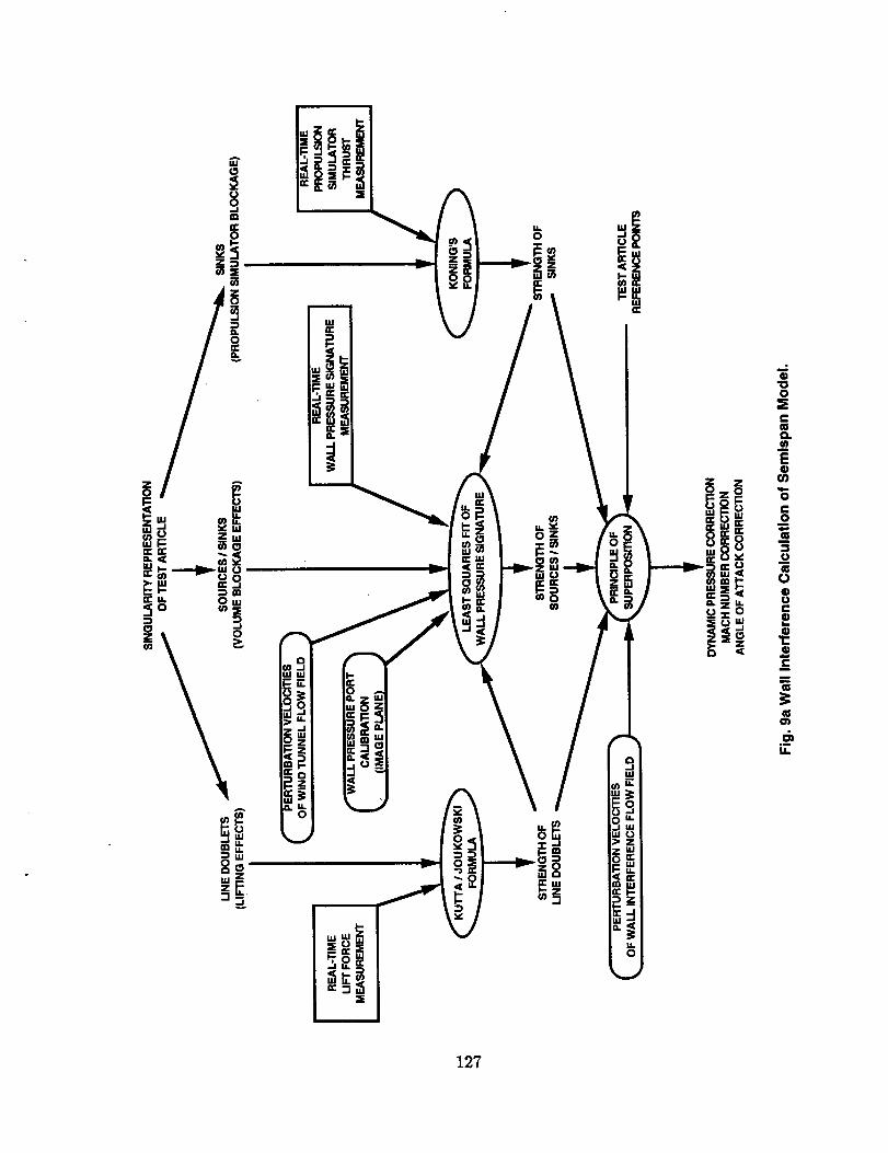
127
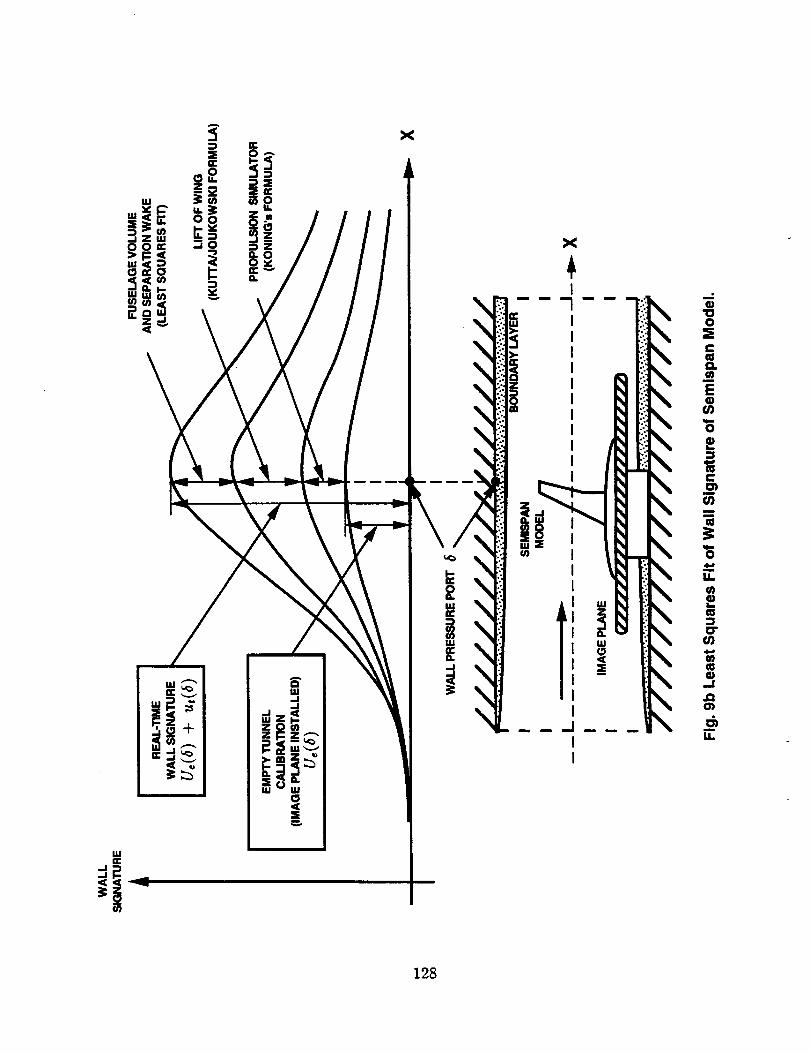
/\
/ iz
III
II
"UO
a.coEO
O
mC
m
mm
a
oi
M
U"
LL
128
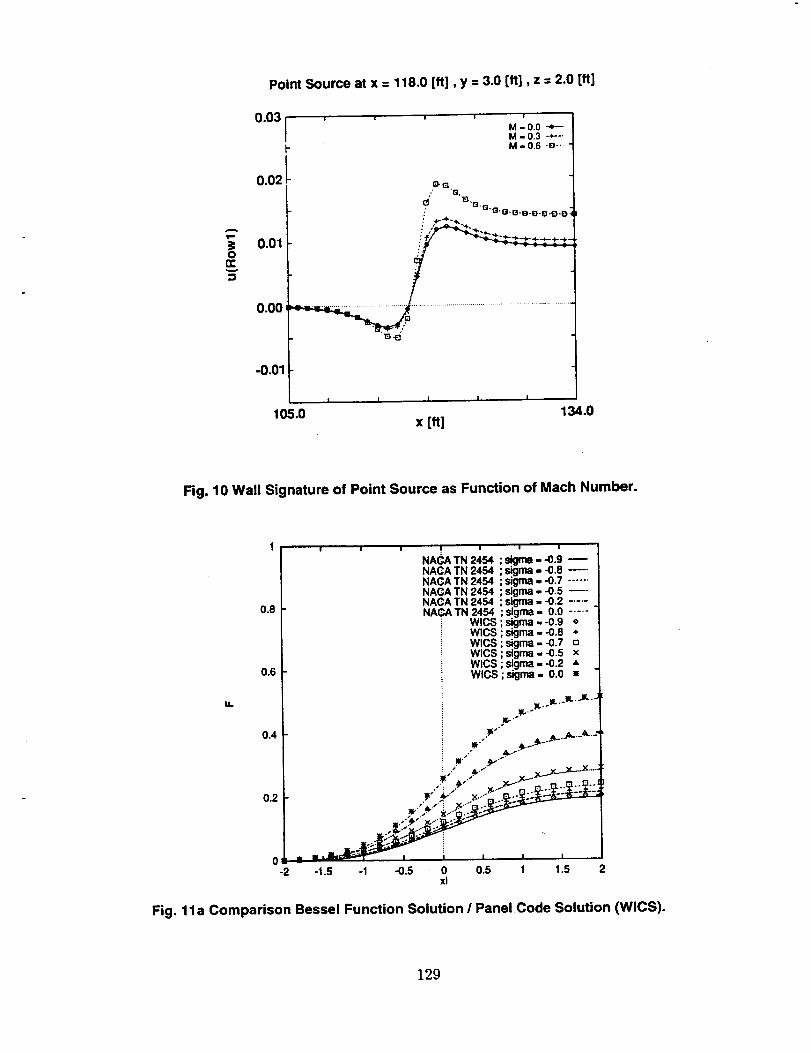
3=O
n-
Point Source at x = 118.0 [ft], y = 3.0 [it], z = 2.0 [It]
0.031 ..... M-0.0M = 0.3 -+---
0.021 M- o.s.0-
0.01
0.00_
-o.011
!
105.0
," "Q,
B-D. g
: "_'Q'B-B O O fOD:' _-_-,. ....
_}-E]
I I I
x [ft]134.0
Fig. 10 Wall Signature of Point Source as Function of Mach Number.
no
0.8
0.6
0.4
0.2
0-2
! i | ! | i i
NA(_A TN 2454 ; sigma, -0.9NACA TN 2454 ; s_ma = -0.8NACA TN 2454 ;sigma = -0.7NACA TN 2454 ; sigma = -0.5NACA TN 2454 ; sigma = -0.2NACA TN 2454 ;sigma = 0.0
WICS ; sigma, -0.9 iWICS ; sigma, -0.8WlCS ; sigma = -0.7WlCS sigma=-0.5 xWIC$ ; sigma = -0.2 AWICS ; sigma = 0.0
Fig. 11a Comparison Bessel Function Solution / Panel Code Solution (WlCS).
129
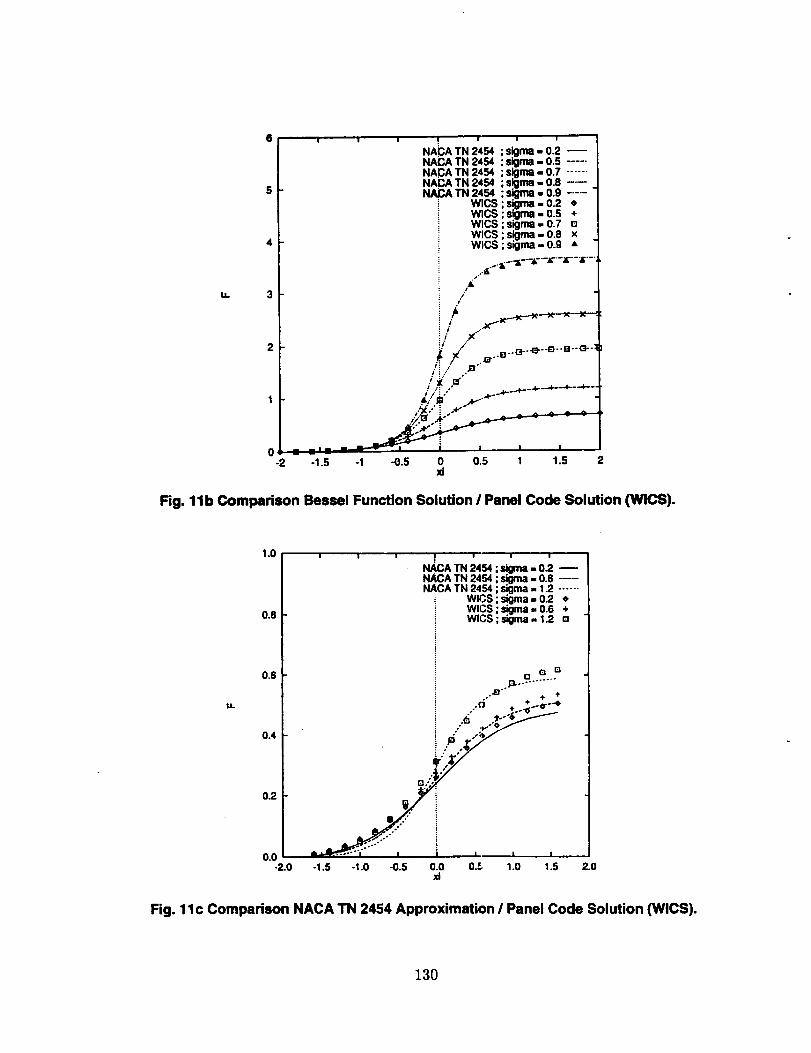
u. 3
2
NACA TN 2454 ;slNAGA TN 2454 ;siNACA TN 2454 ;slNACA TN 2454 ; siNACA TN 2454 ; sl
WlCS ; siWlCS ; slWlCS ; siWICS ; siWICS ; si
i !
]ma = 0.2|ma - 0.5 .....jma - 0.7 ......]ma - 0.8Bma - 0.9 ...._ma - 0.2 *0ma = 0.5 +oma - 0.7 ogma = 0.8 xgma - 0.9 •
./
i/ f_/ .x"
;_/.e.oS..(a--_"O"B"GP"
i i ..""
0 -- ==i.= -- --.,I I I
-2 -1.5 -1 -0.5 0 0.5 1 1.5 23d
Fig. 11b Comparison Bessel Function Solution ! Panel Code Solution (WlCS).
U.
1.0
0.8
0.6
0.4
02
I i i i
NAC& TN 2454 ; sigma - 0.2 --NACA TN 2454 ; sigma. 0.6 ....NACA TN 2454 ; sigma - 1.2 ......
WICS ; sigma - 0.2 •WICS ; sigma. 0.6 +WlCS ; sigma - 12. o
0.0-2.0 2.0
...p....q "..-"o. + 4"
..-_] + ._--o --'e
• . ¢"._-'_/
I ../ i
°.-°" [
I ! !
-1.5 -1.0 -0.5 0.0 0.!; 1.0 1.5xt
Fig. 11 c Comparison NACA TN 2454 Approximation / Panel Code Solution (WlCS).
130
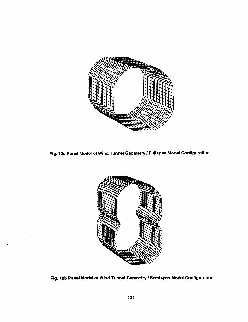
Fig. 12a Panel Model of Wind Tunnel Geometry/Fullspan Model Configuration.
Fig. 12b Panel Modal of Wind Tunnel Geometry / Semispan Model Configuration.
131
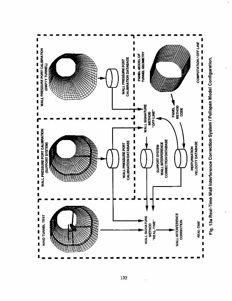
132
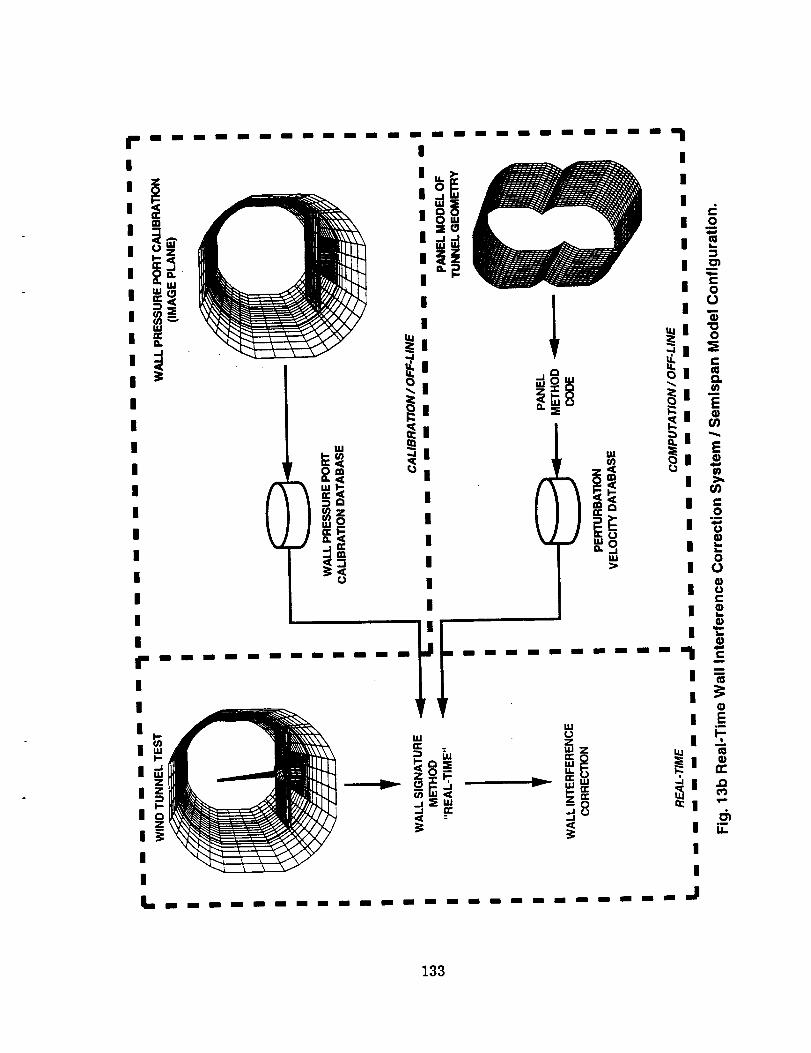
133
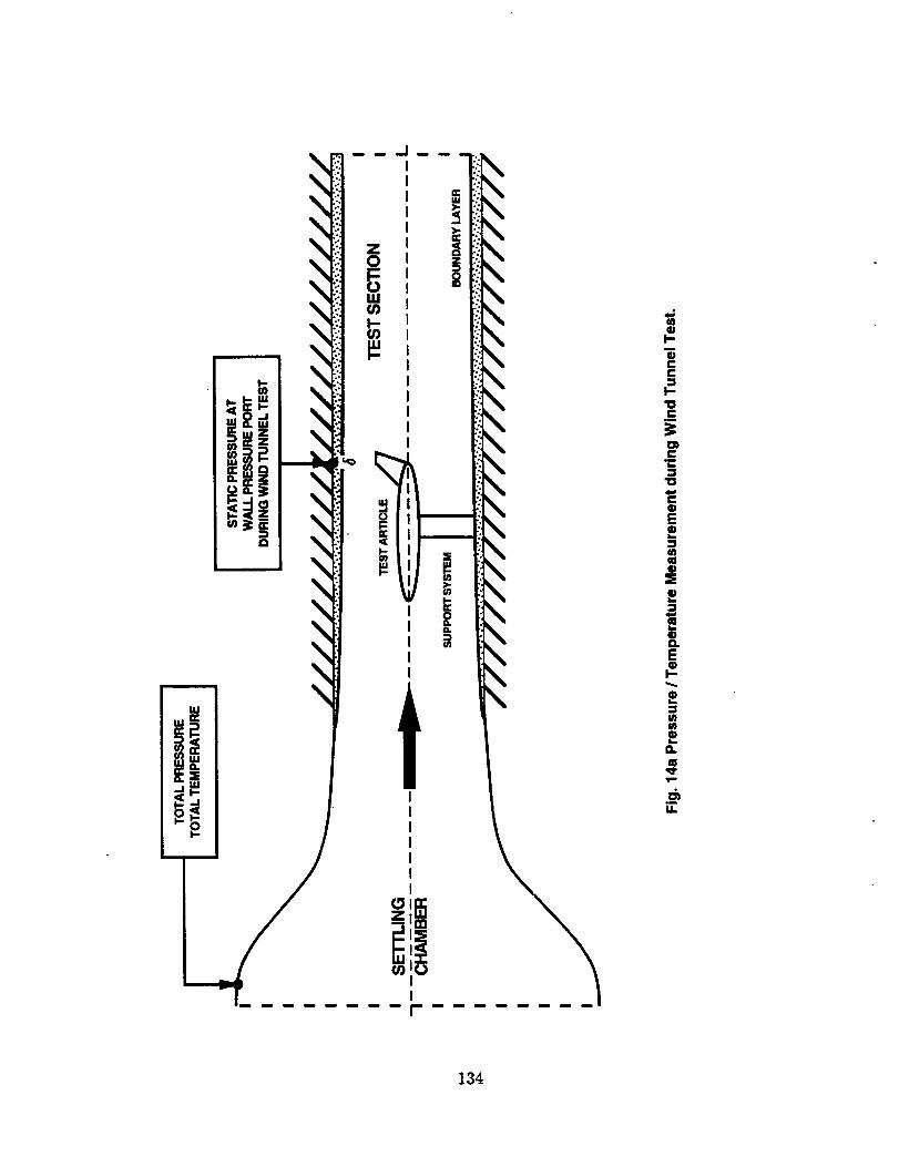
i
M0
m0CC
I--
"U
3"0
C0
E8MmQ
@L_
E0
E0I--
D.
U.
134
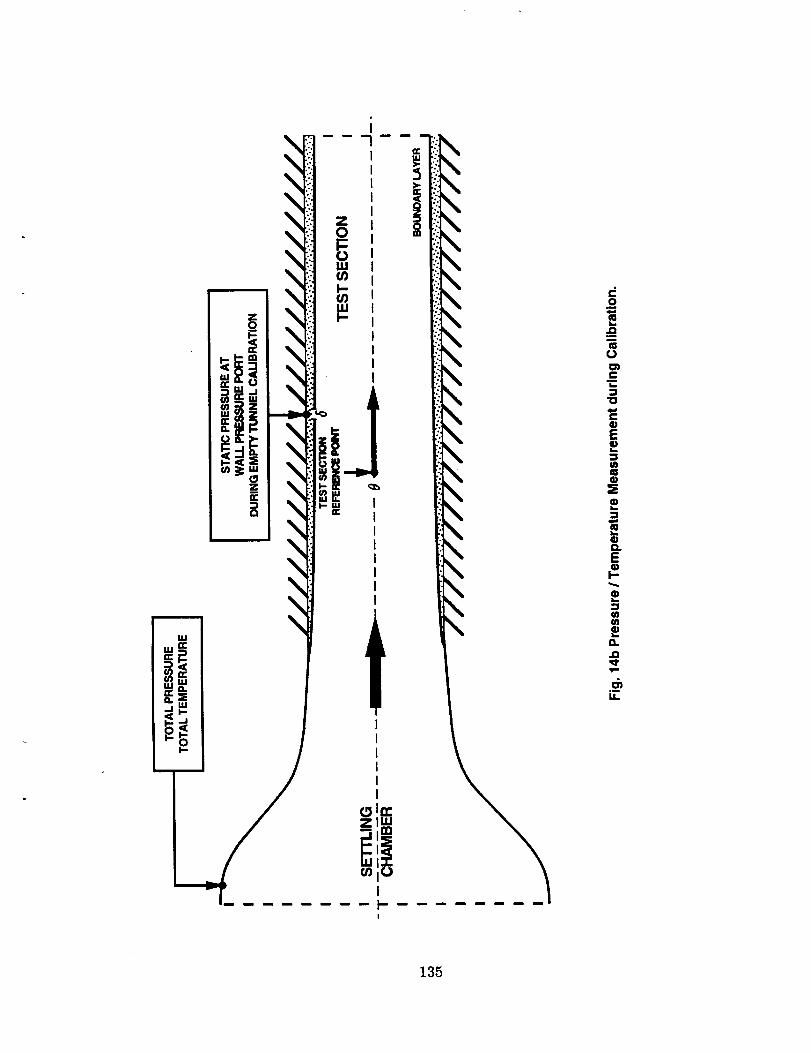
\
In-
2
.0
a.
u.
135
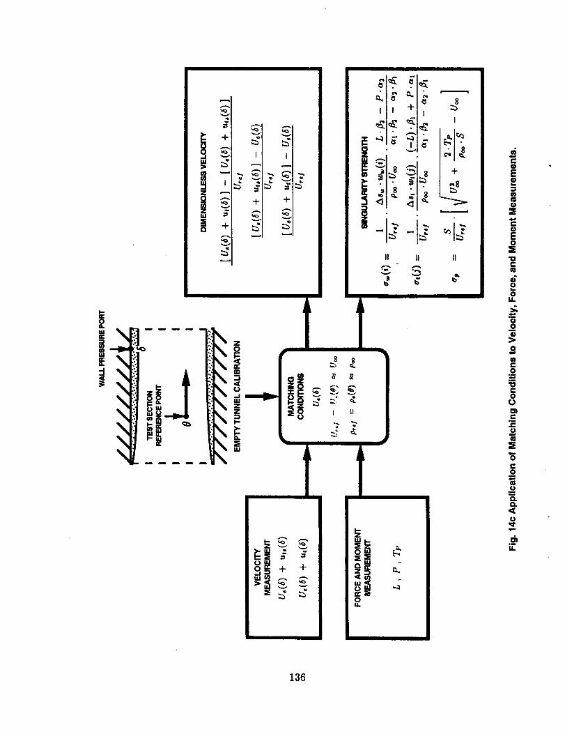
""- , ,,_Yl,,,_a i i,.._ i
9
014.
I I -I-
Aow
8 "
<1 <I
I
_1_._,1_
+
_ _1_II II II
• w o,e%
e,
E
i-IDE0
e.
0i1
u
_o@
0
e-o
"0_..0
U
cm
J_Um
C_o
<
i1
13G
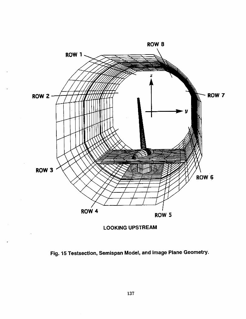
ROW 1
ROW 4
ROW 8
ROW S
ROW 7
ROW 6
LOOKING UPSTREAM
Fig. 15 Testsection, Semispan Model, and Image Plane Geometry.
137
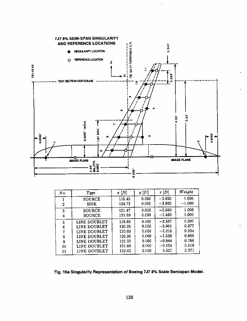
7J7 8% SEMI-SPAN SINGULARITYAND REFERENCE LOCATIONS
• SINGU.AFgTYLOCATION
O RB=B_ENCEL(T_ON
TESTSECTIONCB,ffEFU_
I
IMAGEPLANE IMAGEPLANE
No.
I2
34
567891011
Type z [ft] y [f_,] z _t] WeightSOURCE 116.45 0.000 -3.920 1.000
SINK 124.73 0.000 -3.920 -1.000
SOURCE 121.47 0.000 -2.930 1.000SOURCE 121.69 O.CO0 -1.430 1.000
LINE DOUBLETLINE DOUBLETLINE DOUBLETLINE DOUBLETLINE DOUBLETLINE DOUBLETLINE DOUBLET
119.89120.25120.60120.96121.32121.68122.03
0.0000.0000.0000.00002000.0000.000
-3.587-2.901
-2.216-1.530-0.844-0.159
0.527
0.9970.9770.9340.8660.7660.6190.371
Fig. 16a Singularity Representation of Boeing 7J7 8% Scale Semispan Model.
138
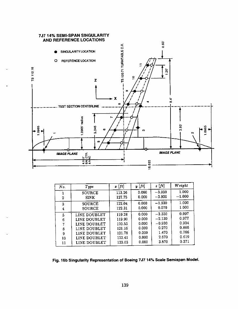
7J7 14% SEMI-SPAN SINGULARITYAND REFERENCE LOCATIONS
• SINGULARITY LOCATION
O REFERENCE LOCATION
... TEST SECTIONCENTERLINE
IMAGE PLANE
No.
1
2
3
4
56
7
8
9
1011
Type z [ft] y [ft] z [ft] Weight
SOURCE 113.26 0.000 -3.920 1.000
SINK 127.75 0.000 -3.920 -I.000
SOURCE 122.04 0.000 -1.930 1.000
SOURCE 122.31 0.000 0.070 1.000
LINE DOUBLET
LINE DOUBLET
LINE DOUBLET
LINE DOUBLET
LINE DOUBLET
LINE DOUBLET
LINE DOUBLET
119.28
119.90
120.53
121.16
121.78
122.41
123.03
0.000
0.000
0.000
0.000
0.000
0.000
0.000
-3.330
-2.130
-0.930
0.270
1.470
2.670
3.870
0.997
0.977
0.934
0.866
0.766
0.619
0.371
Fig. 16b Singularity Representation of Boeing 7J7 14% Scale Semispan Model.
139
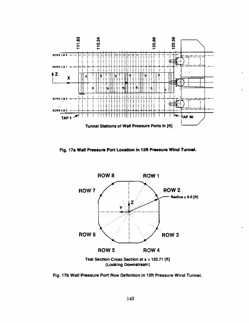
,lira
ROWS I & $ ....
ROWS 2 & 7 ....
Z X
v,- 04 04
i' F i [iriiiirtitTiTiit[iiii [ i i t"F _:=1..... ]-:-....., i ! i iiii!i!Ji!ili!iiiiiiiii i i-E _2._i.... j._-J_.l.-. J-.M.L.L-L.IM. LL-LJM, LL _-L-I.L._-J..J-I.I-._. M.--_ .................
I I t II111111111 IIIIIIIIIII I I I
ig i 'iiiii=iiigiiiii,ii _ i i),/1, ,!il!l,n,,li,,Iilili i!II_--rTT__-_-_÷r,÷__-_+_-_E_-I----I.......Ill i _Hi i i_liti i i Bll i i Bilili i i_ll i _.lil
,_ ! ill!!i':il_l_'!iiiI,!iii!Iilii!!H i _lil,t I I IIIII11111111111111111 I I I
RO_ _ _ 6 .... [ ]-- I [ T i ]" [l i I TF[TiTITiTIqTiTiqTTq-_ _,-r 1-- i i i i iiiiiiiiiiiiiiiiiiiiii i i'v_J_L i_.... , , , ., . ° , , ° , o , , o , i , . '-.-. °_° .
ROWS4& 5 .... I---I--- F--I---;-t-t--I- 4-t-I-I-4--I-4. H 4--t-I-&F-I- 4-,l-.l--.-l.--.-l---._-4---
tapl._,' ! i i i!iiiiiiiiiiiiiiiiiiii i i i b_-TaP30
I /Tunnel Stations of Wall Pressure Ports in [ft]
Fig. 17a Wall Pressure Port Location in 12ft Pressure Wind Tunnel.
ROW 7
ROW 6
ROW 8 ROW 1
S
• ', j
y L
_,/ /
/
., .. ROW 2,'" ." _- Radius = 6.0 [ft]
ROW 3
ROW 5 ROW 4
Test Section Cross Section at x = 120.71 [ft]
(Looking Downstream)
Fig. 17b Wall Pressure Port Row Definition in l!:2ft Pressure Wind Tunnel•
140
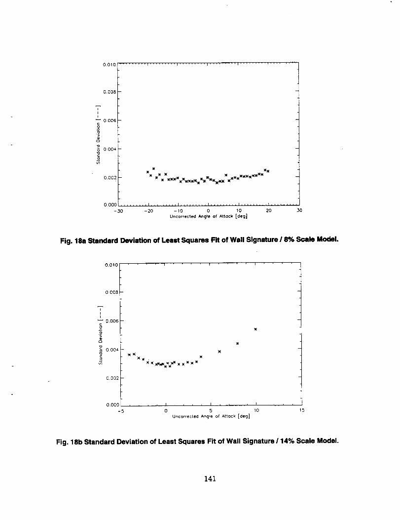
"TII
o=o
-£.
oLf)
O.OtO
0.008
0.006
0.004
0,002
0.000
-30
......... I ......... I ......... I ......... I ......... I ........
-20 -t0 0 tO 20
Uncorrected Angle of Attack [deg]
3O
Fig. 18a Standard Deviation of Least Squares Fit of Wall Signature 18% Scale Model.
0.010
0.008
'T"II
0.006
_ 0.004co
0.002 I
0.000 /
-5
I ! i
0 5 10 15
Uncorrected Angle of Attack [deg]
Fig. 18b Standard Deviation of Least Squares Fit of Wall Signature/14% Scale Model.
141
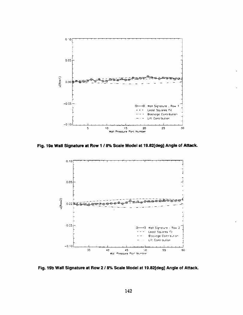
0_0
0.05
v
-0.05
-0 tc
....-.----_-_;_-.._-..-:1111-_
, , I , ,
5 3O
Wolf Signature ; Row 1
-- - Least Squares Fit
..... Blockage Contribution
.... Lift Contribution
] I , , ; I
10 15 20 25
Wotl Pressure Port Number
Fig. 19a Wall Signature at Row I /8% Scale Model at 19.82[deg] Angle of Attack.
v
0.10 t ' i I r ' _ 1 r ' i
0.05 F
r
0oo._-.-=--:z_ ; _ ...................
E-0 05 I
r
10
35 40 60
G"_q Walt Signature ; Row 2
- -- Least Squares _'it
- - • 81ockage Contribution
-- " L;ft Contnbution
I , , _ , r L _ , ,
45 !!,0 55Wail Pressure Port Number
Fig. 19b Wall Signature at Row 2 / 8% Scale Model at 19.82[deg] Angle of Attack.
142
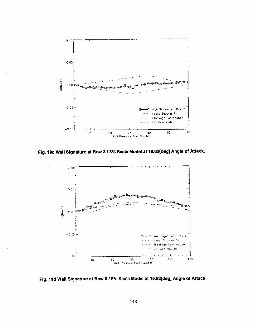
r I .... I '
0 I0 I _ ' ' I .... r-" ' ' ' l
E
0.05 I
F
L- --_-_-_-__............................... - -
o.oo __._ _- ..... _- _,_-=- ....- ............
-0.05ES----E2 Wali Signolure ; Row 3
- - - Least Squares Fit
..... 81ockoge Contribution
..... Lift Contribution
, , , I , , _ , I , , , t 1 L _ _ T ! , L , r I _ , _ ,
65 70 75 80 85
Wall Pressure Port Number
9O
-0.10
Fig. 19c Wall Signature at Row 3 / 8% Scale Model at 19.82[deg] Angle of Attack.
0.10
0.05
0.00rr
' ' ' I ' ' ' I " I .... I " ' I
--005 _ Wall Signature : Row 6
L - - - Least Squares Fit
I .... Blockage Contribution
P .... Lift ContributiOn
-0101 J , , F , L , , I , , , J I , , , , I , , , , L , , , , ,
155 160 165 170 ! 75 180
Woll Pressure Port Number
Fig. 19d Wall Signature at Row 6 / 8% Scale Model at 19.82[deg] Angle of Attack.
143
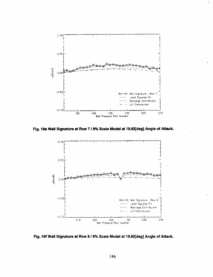
010
0.05
o 0 O0
D
-005.I
-0.10 , , , I
185
' ' ' I ' ' ' r I
,,I,,,,I
_] WoII Signature ; Row 7 J
- -- Leost Squores Fit J
..... 810ckrge ContributiOn
..... Lift Colnt riDution
K i I i i i i I i i _ i
190 195 2:)0 205 210
WOII Pressure Port Numb,;r
Fig. 19e Wall Signature at Row 718% Scale Model at 19.82[deg] Angle of Attack.
I I ' ' ' 1 ' I I
0.05
ooo
-0 05
-0 10
[_'-----g WOH Sicjrcture ; Row 8
- -- Leos! Squores rlt
.... Blockage Cont _;bution
.... Lift Contribut,On
2 _5 220 225 : 30 235 240
WoIt Pressure Port Number
Fig. 19f Wall Signature at Row 8 / 8% Scale Model at 19.82[deg] Angle of Attack.
144
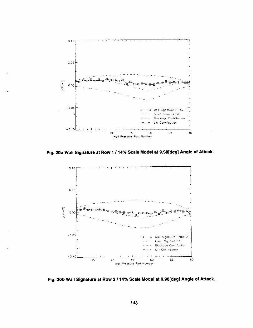
0_0
0.05
o 000re
/
-0'05 I _ WEHI Signature : Row 1
Least Squares Fit
..... Blockoge Contr_'bution
..... Lift Contributior_
-0,101 , , , I , , , , ! , , , , I , , , , I , , , , I , , , ,
5 10 i5 20 25
Wall Pressure Port Number
30
Fig. 20a Wall Signature at Row I / 14% Scale Model at 9.98[deg] Angle of Attack.
I ' ' I ' ' ' I ' I I
0.05
o_ 0.00
v
-005
-010
i
WoH Signature ; Row 2
- - - Least Squares Fit
.... Blockage Contr_ution
.... Lift Contribution
55 40 45 50 55
Wall Pressure Port Number
60
Fig. 20b Wall Signature at Row 2 / 14% Scale Model at 9.98[deg] Angle of Attack.
145
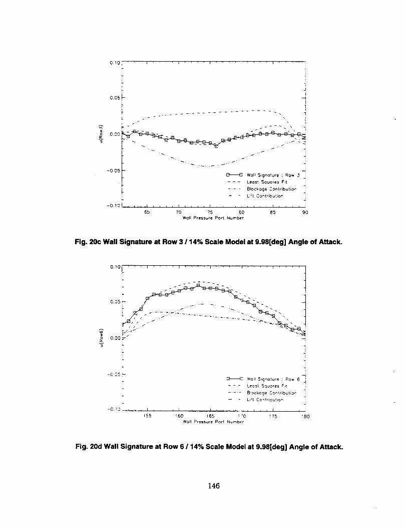
010
0.05
o 0.00n-
--0.05
-0._0
' ' I .... I [ ' '
/
[3-_--E] Wall Signature ; Row 3
--- Least Squares Fit
..... Blockage Contribution
..... Lift Contribution
i i l i J r l I I l = l I I l i i , i = i i P = = = = ,
65 70 75 _0 85 90
WoII Pressure Port Number
Fig. 20c Wall Signature at Row 31 14% Scale Model at 9.98[deg] Angle of Attack.
O. tO
005
_. o.oo
I I ' ' I I .... I ' '
--/
-0 05
C_-{] Wall Signature ; Row 6
I Least Squares Fit
..... Blockage Contr;but;On
-- - LJt Contribution
-0 10 , , , I , , r , r , , , b I , T , , , , , , I , , , ,
155 160 165 T '0 175
Wall Pressure Port Number
8O
Fig. 20d Wall Signature at Row 6 / 14% Scale Model at 9.98[deg] Angle of Attack.
146
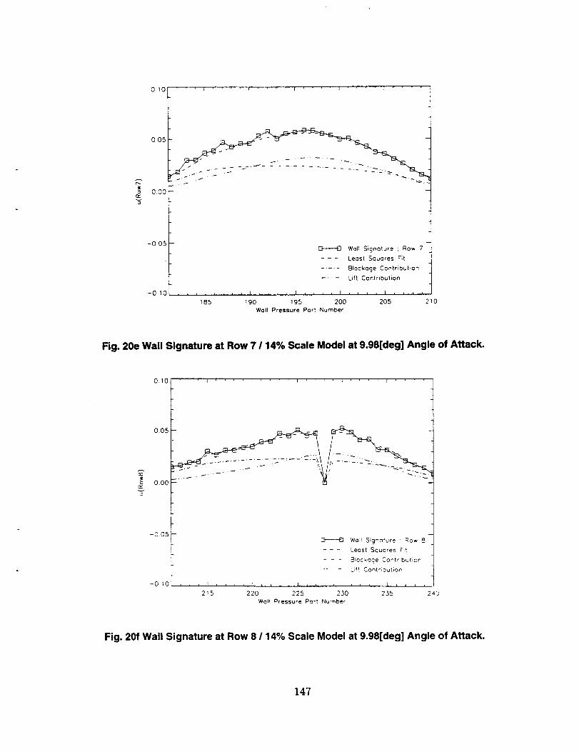
0.10
OO5
o 0.0Ce,-D
-005
-0.10
i .... i • ' ' I ' ] .... f ' '
m
Wail Signoture ; Row 7
--- Leost Squores Fit
..... Blockage Cor_tribution
..... Lift Contributior_
i l J I h i J i I , l i _ I i i i , I l l I _ l , i _ l
185 190 195 200 205W011 Pressure Port Number
!1o
Fig. 20e Wall Signature at Row 7 / 14% Scale Model at 9.98[deg] Angle of Attack.
0.10
0.05
"o ooot_
1
-005 I _ WOII Signoture ; Row 8
- - - Leost £_uores Fit
- - - BPockoge Cor_tribution
.... Lift Contributior_
-0 10/ , _ , ; , , , , T _ , _ , I _ , , , I , I , , _ ,
215 220 225 250 255 240
WO_ Pressure Port Numbe¢
Fig. 201'Wall Signature at Row 8 / 14% Scale Model at 9.98[deg] Angle of Attack.
147
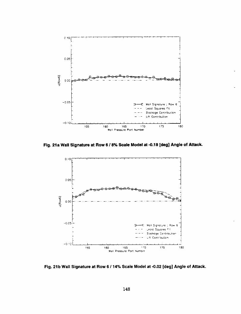
005 i
-005
-0.10
{_ WoII Signature ; Row 6
- -- Least Squares Fit
..... Blockage Contribution
..... Lift Contribution
, , , 1 , , , , I , , , A i , L i I .... 1 , , ,
155 160 165 170 175
Woll Pressure Port Number
180
Fig. 21a Wall Signature at Row 6 / 8% Scale Model at -0.18 [deg] Angle of Attack.
0.10
0.05
_o o.oo
D
--005
' ' I l ' ' I ' ' ' ' ] "
1
_3"_"=-_] Woll Signature ; ROW 6
- - - Least Squares rlt
..... Blockage Contribution
.... Lift ContribuUon
155 160 165 I 70 175
WOIP Pressure Port Numb,tr
80
Fig. 21 b Wall Signature at Row 6 1 14% Scale Model at -0.02 [deg] Angle of Attack.
148
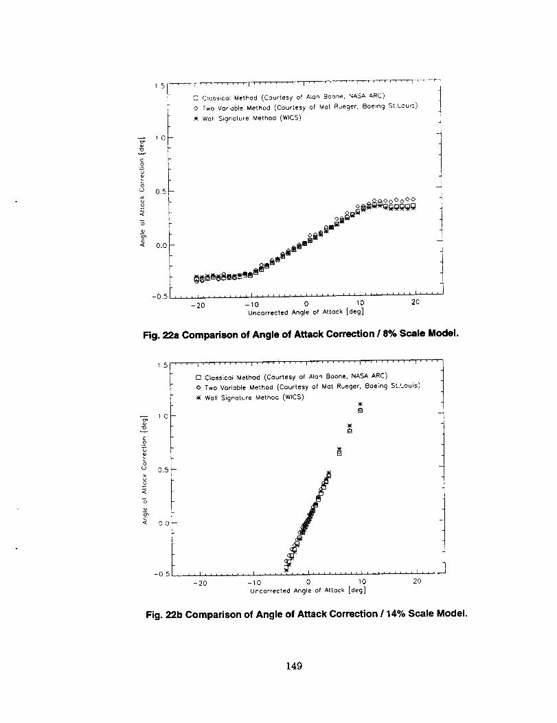
15
g
o
_D 0.5
o.o
-0.5
E] Classical Method (Courtesy of Alan Boone, NASA ARC)
O TwO Variable Method (Courtesy of Mot Rueger, Boeing St.Louis)
Wall Signature Method (WlCS)
___0000 O0
liil m_il !
-20 -tO 0 10 20
Uncorrected Angle of Attack [deg]
Fig. 22a Comparison of Angle of Attack Correction / 8% Scale Model.
_.5
1,0
g
O
0.5
o
00
-05
.... I ......... I ' ' ' '" ' ' ' ' I .... ' ' ' ' ' I ' ' ' ' ' ' ' ' ' I ' ' '
O Classical Method (Courtesy of Alan Boone, NASA ARC)
O Two Variable Method (Courtesy of Mot Rueger. Boeing St.Louis)
WoN Signature Method (WICS)
-20 -10 0 lO 20
Uncorrected Angle of Attack [de9]
Fig. 22b Comparison of Angle of Attack Correction / 14% Scale Model.
149
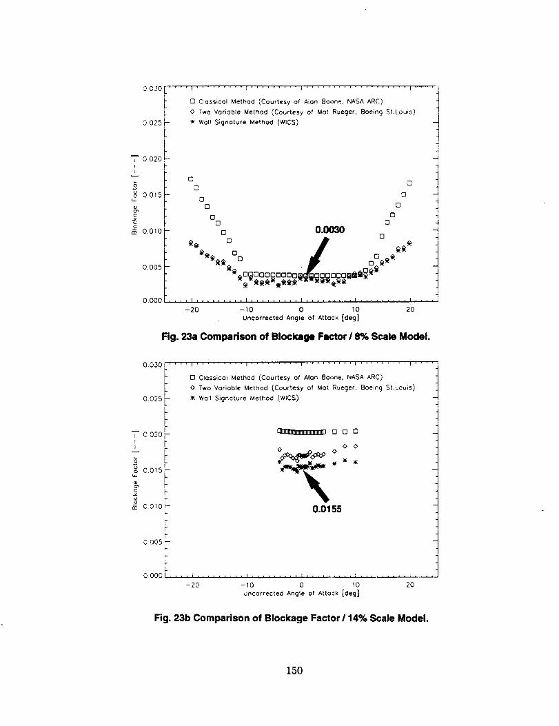
0.050
0025
_" 0020.
' L&
0.015
: f0.010-
0.005
0.000
--T ' ' ' I ......... I ......... I ......... I ......... I ....
O Clossicol Method (Courtesy of Alon Boone, NASA ARC)
O Two Vorioble Method (Courtesy of Mot Rueger, Boeln 9 St.Louis)
Woll Signoture Method (WlCS)
O 0[]
[3 O
[] O
0 C_rn 0
o 0.0030
_ 0 I []
___ 0 o J 0
%_o_ooo_oooo_'oooooo_m_ @
-20 -10 0 10 20
Uncorrected Angle of Attock [deg]
Fig. 23a Comparison of Blockage Factor 18% Scale Model.
0.030
0,025
'_' 0 020
sF>o.o_5
o.x
0010
0005 I
p-
' ' ' ' I ......... I ......... I ......... I ' ........ I ' ' '
[] ClossIcol Method (Courtesy of Alon Boone, NASA ARC)
O Two Voriobte Method (Courtesy of Mot Rueger, Boeing St.Louis)
Woll Signoture Method (WlCS)
_ O 0 0
o oo
0.0155
0.0001 .... i ......... _ ......... t ......... i ......... i,.....,.__
-20 -I0 0 10 20
Uncorrected Angle of Atto:k [deg]
Fig. 23b Comparison of Blockage Factor/14% Scale Model.
160
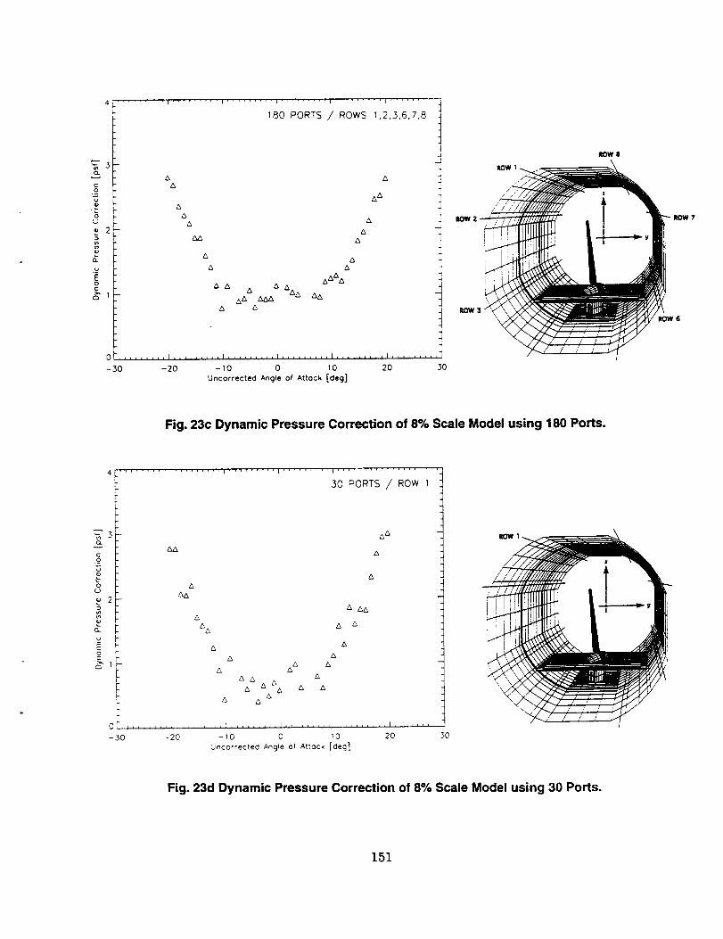
&
o
0J
n
E
......... 1 ......... i ......... i ......... i ......... } ........
180 PORTS / ROWS 1,2,3.6,7,8
AA
A A
AA &
-30 -20 -I0 0 10 20
Uncorrected AngLe of Attack [deg]
q
mow 8
// ,/
3O
IK_7
ROWG
Fig. 23c Dynamic Pressure Correction of 8% Scale Model using 180 Ports.
3CL
O
2
¢U
iC3
......... I ......... r''' ...... I ......... I .... _ .... I .........
.30 PORTS / ROW 1
AA
&
A
Az_A 1
A AAA
I Z_& & A5, &
A ,& ,&A 1i & A D'A A Z_A A A
--.30 -20 - _ 0 0 _0 20 30
Uncorrected Angle of Attack [deg]
Fig. 23d Dynamic Pressure Correction of 8% Scale Model using 30 Ports.
151
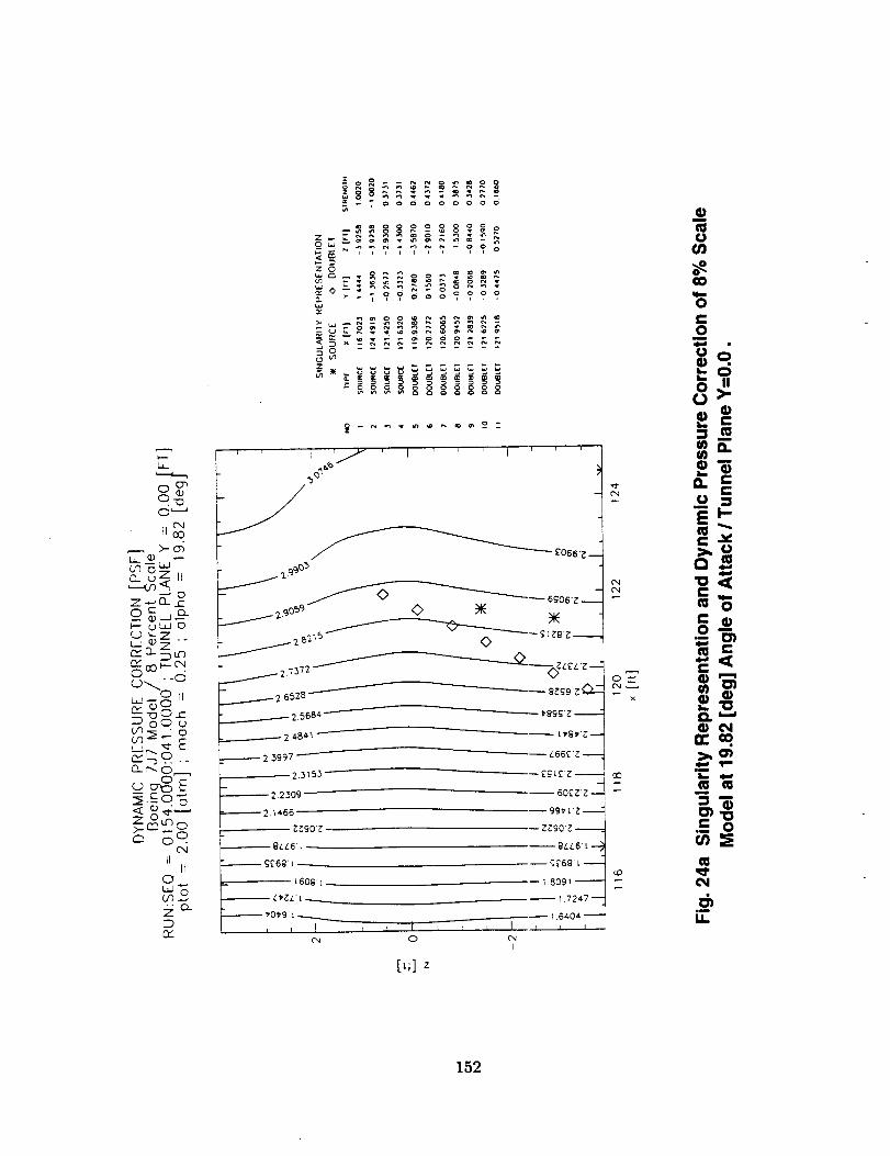
•- i o o o o 0 o o o 0
ZO
- 7?? o_???
0
____--"--E066"_--
/ 27372 _--__-_--_"----_L£L "_--:
/ 2.6528 -'"- 8_gg '_
_.__,_.___--.----2,5684
_._.___._..._..-.---2_84_°
_2.3997
2.3_53-
_2.2309
=-----'_--2._466
0_9_ .
O4
,, _ '_ _ , _ !0 c'_
I
[_;] z
O4
C_lO4
_g_._._....:
_8#_
L65£Z--
_E90'_
8LL6"_
--g£68'_
- _.7247--
1.6404--
m
o
0c-O
mm
o 0
0 II
l-
O_
e-
t¢1 _'1
.__ 0
u
152
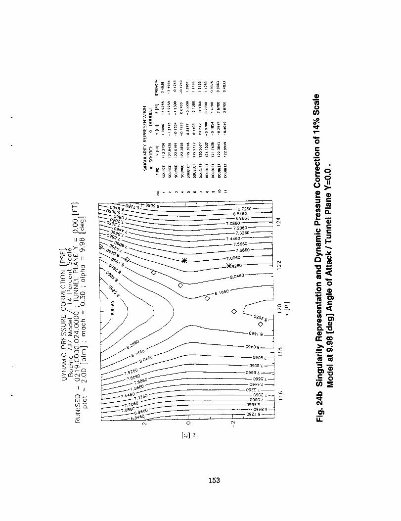
I-'--L.L
O_
LJ_--
_Z--
0_" II
0 - ¢-_
L__" r-_ O .-
_cOa- i.._J<50_
ZO_O)- ED c,,l 0c: o_
II tl
0"---,1..,.i0
ZDIZ
_=???-.---ooo
-_oo_°_°,,,,
o
<>
- 099L B
(_ c,JI
h}] z
£xl¢',1
x
uD
t,D
c
m
._0 C
C
c,_
_- 0.0_ _)t_
.,., e-
¢),'-,
Q.'O
n'co
m m
.E 0
.i
153
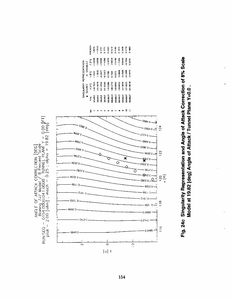
."_D
0"--'
>'- 0'_,-.--, (])
U.J _ _ II
__ _UJO
w o- _ u.3
,<-__oOu
_- r-- Or.__, ,
Z CI_O if3 0
< S°O4
IL
11
2 _
C12
Z 0
N__o:--
>-
Z
_ _ _ _ _ _ _ _ _ - _
_ww_w
_ _ Ol 0 l 0.0742 --
-- gg_,O 0--_ 0.0485 ""
i I I, r _ I , , I , , _ 1 i =
I
[_1
C'4
O4
O=--f'4_
x
CO
UD
(I}
L_
U "
U
< cC
o l-
u
U
m 0
0--
--<[:
rr_.>,01
m
='_
U
m
I,I.
154
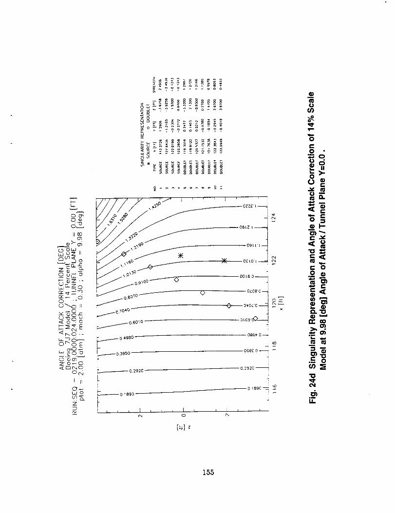
zO
_-__;_ _
"z'D..
d_
OObJ
_- I1) _j--
OOL_O
_z.-_-Zo °_'°°"'-----__-_ _" _0_0_ . 0 O.
._. _o
o _ o _ _0.6010
<r'_O --_.. _ _--:,,..,,,=,
°r"o E
70--0
o_
0"_Ld 0
ZDD2
09_'_--
/ix
00_6'0_
o/090 --
0 ol, o/o-
0 L09 _:_-,,_
(-4('-4
._..-.- o.498o o£6_ o-CO
--1
....---.-----0.3950' 0£6£'0_ --
_.---.-----------0.29200.2920 --
4
01890-=--
i i i
_.--._ O. 1890
1
[_] z
o__-x
Or)
"6
=(:;I--
I=
0
e- 0
._-- 0mN"o
u.
155
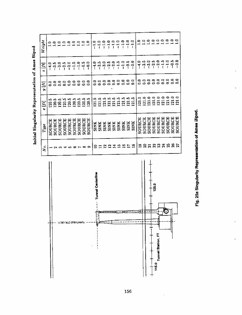
0
gO
<
0
lllllllll
JillJJ]JlilJJ)JlJJ ] J I I J I I I i
o
.m
6
00©©o0©oo
0
c
e0
0"6e.
!!i
-'- I.L'O_L'I:d.LO_"ISVINUrI.L ......... _-.-.'-" .................
T
!l
I
I
l
t
)
o
e-o
{/)
e-e-
t'-
o.me&
qm
0
D
O.
tin,,,
l,t.
156
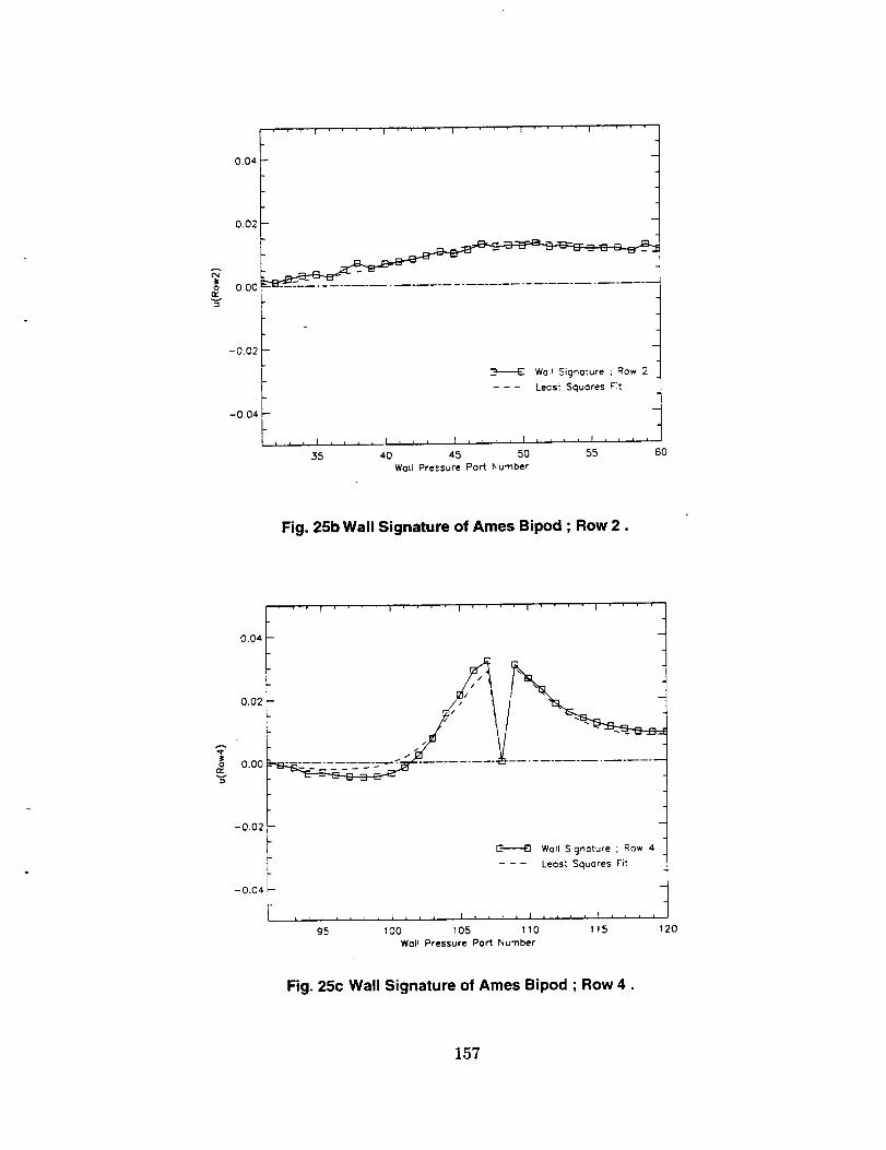
0.04
0.02
0.00
r,-
v
' I .... I t ' I ' I
Wa,_ Signature ; Row 2
--- Leas'. Squares rTt
, , I , t , = I , , _ r I , , , I , t , t I , , ,
35 40 45 50 55 60
Wall Pressure Port h_umber
Fig. 25b Wall Signature of Ames Bipod ; Row 2.
r ' I I .... I .... I .... I .... I ....
k0.04
_" _:0"02 -_ 0.00 .....
"d
-0.02
r'-.-----E] Wall Signature ; Row 4
- - - Least Squares Fit
--0.04
- I 1 I , i " = I t r I I , , ' , I , , , , I , , , ,
g5 100 105 110 115 120
Wall Pressure Port Number
Fig. 25c Wall Signature of Ames Bipod ; Row 4.
157
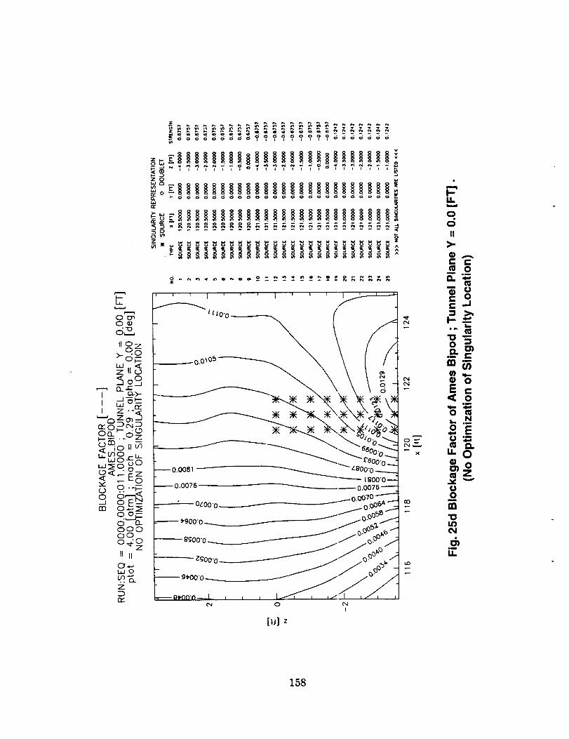
L
0o_O_
dP,II 0 -1
o5wzll_
I c.__.J -- h--
I w o-
o .o..-_
o_.J
rn
d a_OOOOO
o4zoII II
WO
Z
iiiiiiiii 0000000
_° _ 11111|1111111111111111111_ooooooooooooooooooooooooo
' ' ' I ' ' ' I ' ' _ I
---.------_ 0 0 _05 _
____ O'o_
--o.oo _ __oo?oC-___t gO0"O _.Z
--0.0076 0.0076"---':
"- Oz00"0 _ '"-OO0:._O_'__-
8'gO0" __ oDO5: °_
i_I 0 C',,lI
[+_]z
,,¢
(,.,q
_ZX
p,I.I.
00II
>-
e- e-
0
"_ ¢.)e- 0e- ..I
I-- .--'-s_
mN
< o
,_ N
u- O
0
II1
158
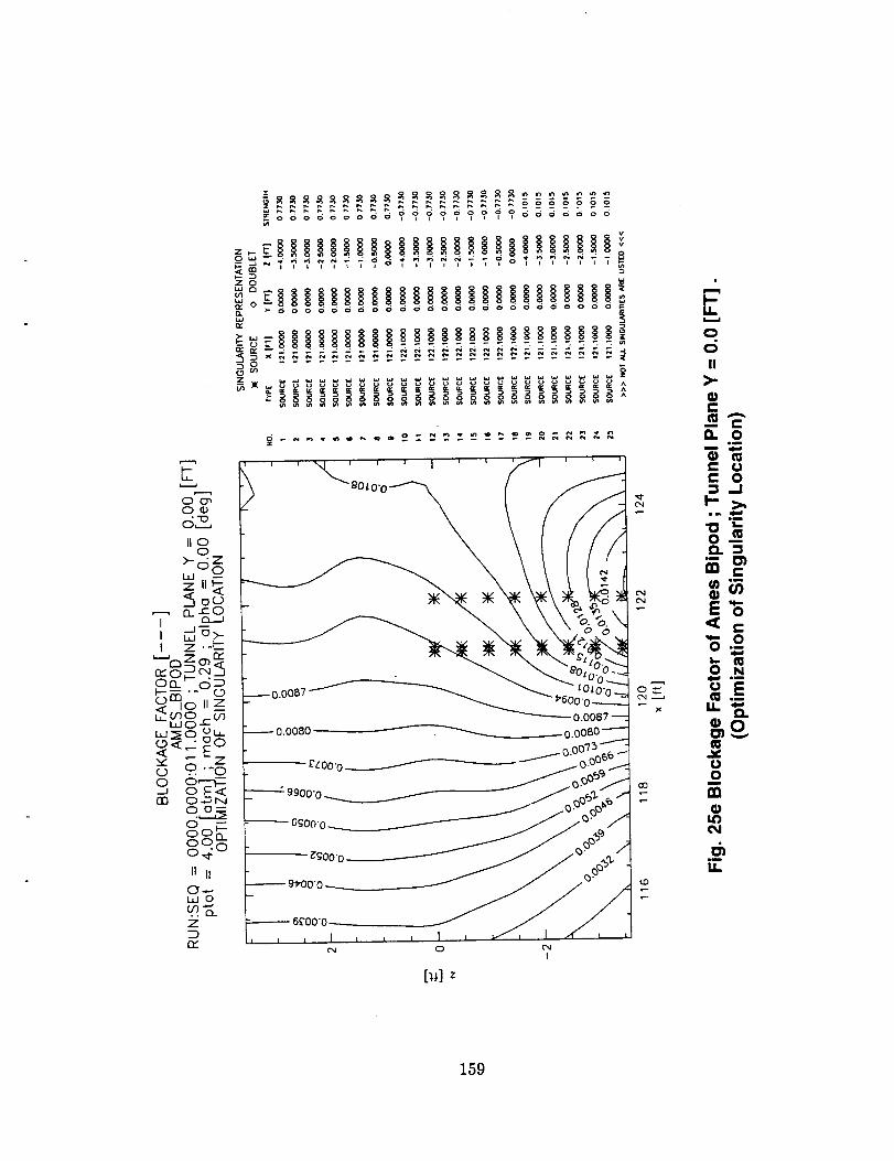
iioo>-cSZLJ 0Z II_
If. c-0
l _o,>_I Z --_--
_oK___ua_ dD_---'" C?
co<,..: NO,_hZ
o .°. "-o
o o_JED
0
o°E°O0
II II(9'..-,I.LIO
Z
n-
[1_,] z
I--
o,5II
--I
t,,-
o0
5_tm
t13
Z
159
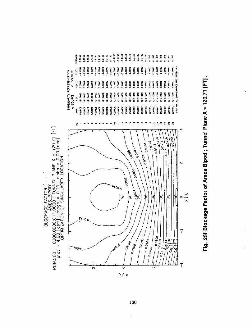
I--
_.'u.0
II 0
x,5_
ZoO
,--, 5&__I o>-
rY o
SN -,I z<,.,'Jo,__,.,
o L,[,..o_8 °o< ,,zE zY
o E'-o_o.
do_
o04li IT
ff
rr
......... _ _ $_$$$$_
ooooooo|lllll
ZO _
_l|llllllll||lllll|_l|llll_-ooooooooooooooooooc_oooooo
' iiiiiiiiiii iiiiiiiiiiiii?
¢',1 0I
(_] z
o ."-,
I
i--
d
IIX
m
D.m
C
b-
0im
E
o!,._
oU
_b_)O)m
Uomttm
t_
160
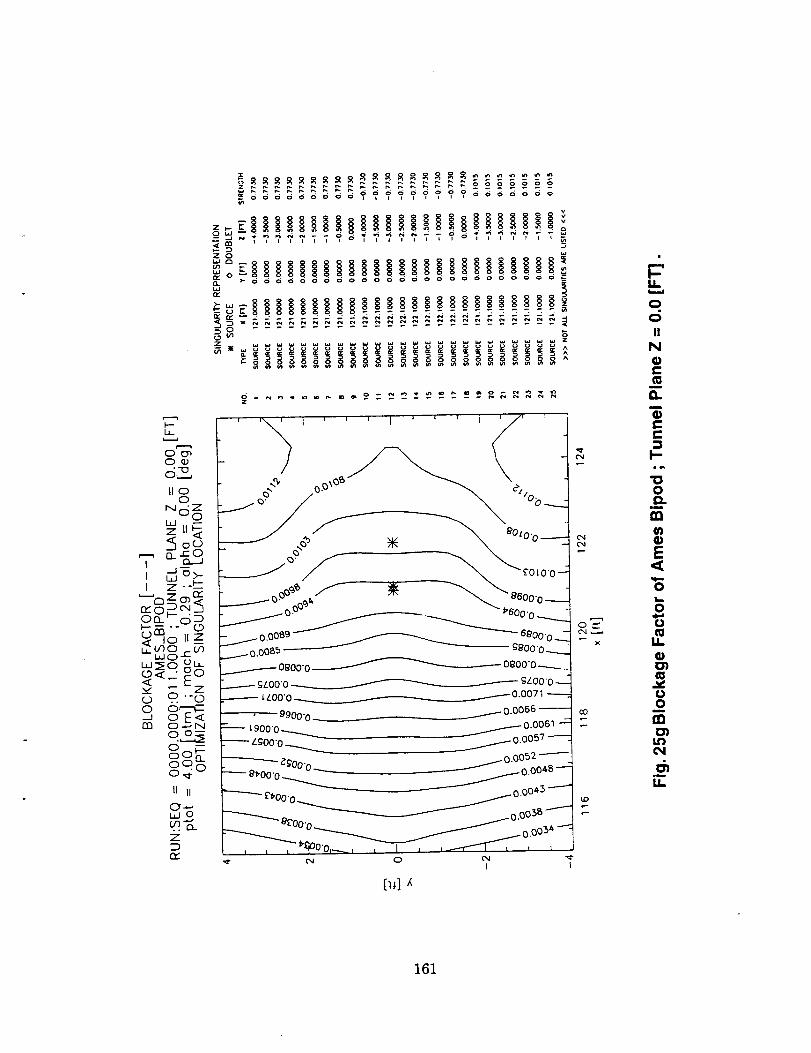
lllllil
ZO
_°_llllllllllllllllllllllll!_-ooo_ooo_oooooooooooooooo
%-
- j_00_ /- _ _ ____----- _" ^_, __ 00"0
_._ 0"_ __ "" _600"0 _,_
/ 0 0089 _" . _ _ 6eOO.o
0.0085 _ g£O0"o -...._
0800"0 _ 0800"0 __
.-----gLO0"O __ g/-O0O
/,z.0:':0 _ 0.0071----=- - 0"0_0"0066
1900"0 _ _.---- 0.0061 "-
.------- Z gOO'o _ _ 0.0057
;---- • " .---- 0.0048 "--:_0__ .... 0.0052 "-"--
£_00"0 _ / 0.0043
-_ _'--o__ ooo_B_"uO "0 " ........
, , , "TuOr-----.,, I , ,_ _ _
I I
o_
x
tL
0
IIN
e-
l
I--
0
em
1=
0i.
00
I.L,_)03
00
I_)OJ
LI.
161
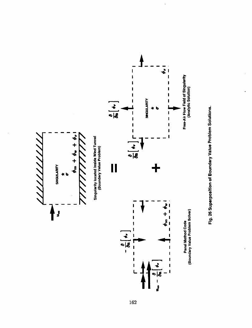
I I -
I I _oi i _==
_g
I I _I ! "
._. -'_
t _0._o
,_ -- II +U tl
b,. m
t- "'' g
,__..._ I I u_
'_l,g , i •I I I o.._
C"I
I ,.--.---, I o
L. _1
t
¢-._o-!
0
E
,IDo
L
Q
IB
"0c-
Om
0
c-O
J
m0
6
(D
°_14.
162
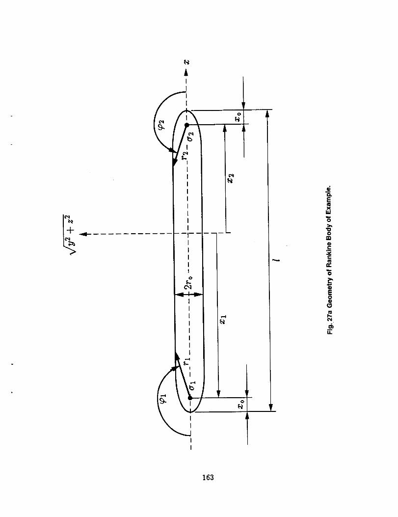
t_
AII
o
IIIIIIII
II
c_
,--4
'r
o
Ex
ILl
0
0m
e-
e,-
rr
0
E0o
m
ot
U.
163
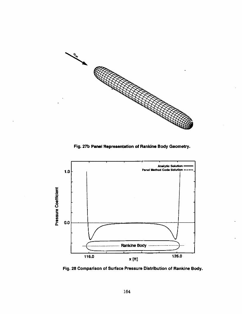
Fig. 27b Panel Representation of Rankine Body Geometry.
e-_o_u
(J
m
n
1.0
0.0
T T "I' T T T
Analytic Solution /
r._nel Method Code Solution ....
...._ ..............................._nk,ne_............................._.....116.0 126.0
x [.]
Fig. 28 Comparison of Surface Pressure Distribution of Rankine Body.
164
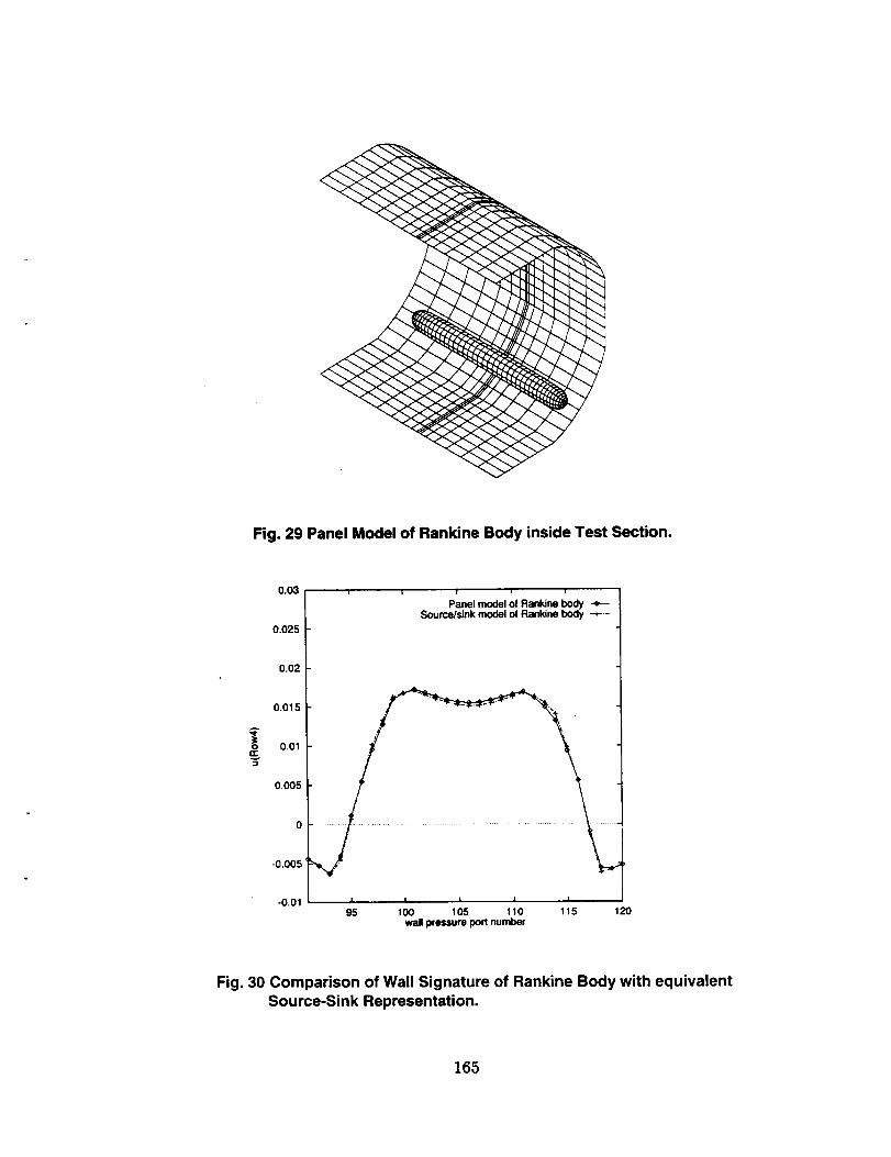
Fig. 29 Panel Model of Rankine Body inside Test Section.
o
0.03
0.025
0.02
0.015
0.01
0.005
-0.005
-0.01
t i !
Panel modet of Rankine bodySource/sink mode4 of Rankine body
95 100 105 110 115 120wall pressure port number
Fig. 30 Comparison of Wall Signature of Rankine Body with equivalentSource-Sink Representation.
165
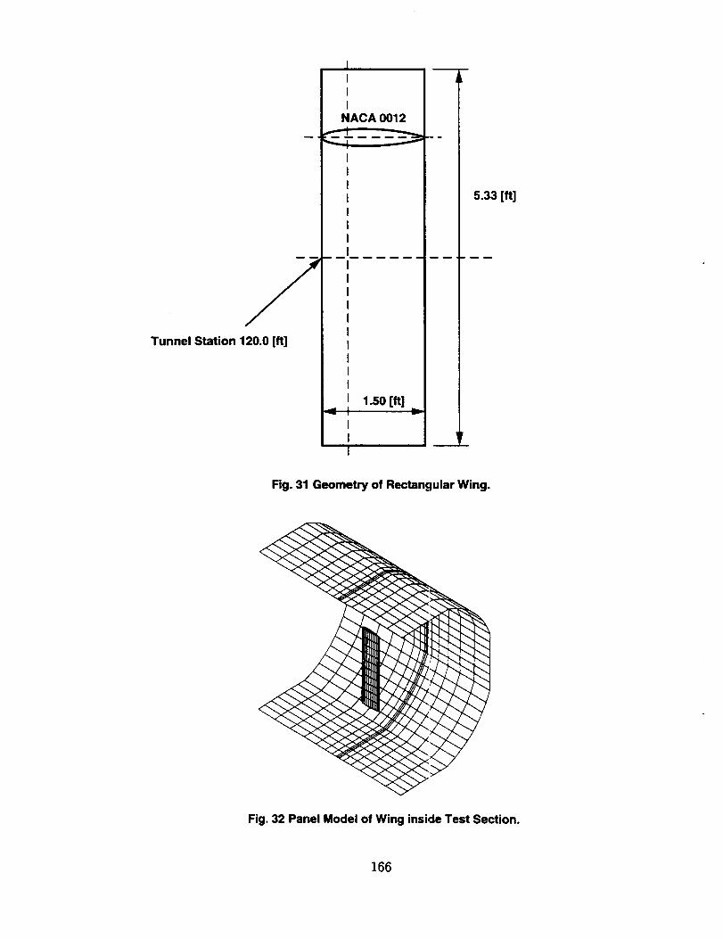
/Tunnel Station 120.0 [ft]
III
NACA 0012
1.50 [ft]v
m
5.33 [ft]
Fig. 31 Geometry of Rectangular Wing.
Fig. 32 Panel Model of Wing inside Test Section.
166
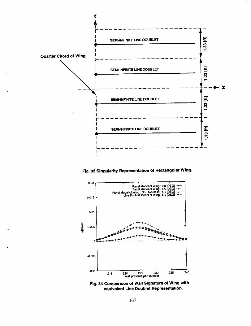
Z
AIfiI SEMHNRNITE LINE DOUBLET
m=
,Iv
I
Quarter Chord of Wing I
I
IT
SEMI-INFINITE UNE DOUBLET
SEMHNRNITE LINE DOUBLET
II
II SEMHNRNrrE UNE DOUBLET
J_w
II
IIi
¢:
y-,
¢:
t_
X
Fig. 33 Singularity Representation of Rectangular Wing.
J=O
(]C
0.02
0.015
0,01
0.005
-0.005
i i i
Panel Model of WingPanel Model of Wing
Panel Model of Wing ; No ThicknessLine Doublet Model ol Wing
!
0.0 [DEG]5.0[DEGI - -s.o[DEG]S.0[DEG]
-0,01 t i I I , I
215 220 225 230 235 240wall pressure po_ number
Fig. 34 Comparison of Wall Signature of Wing with
equivalent Line Doublet Representation.
167
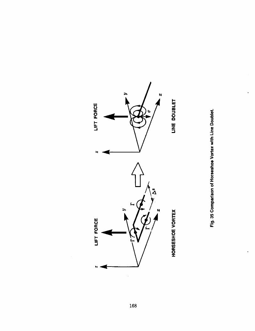
I.UUn-OIL
I=*IL
--I
.3
I-.i.Jm
0
.iZm
,=.J
X.iI-
0
Iii031::O*Jiii
IZ:03C
_w
oC3oc-I4-
x
o
Qo
J_cffowL_
o3_
"6coM
mD.E0
168

O
O
O
O
Ii
169
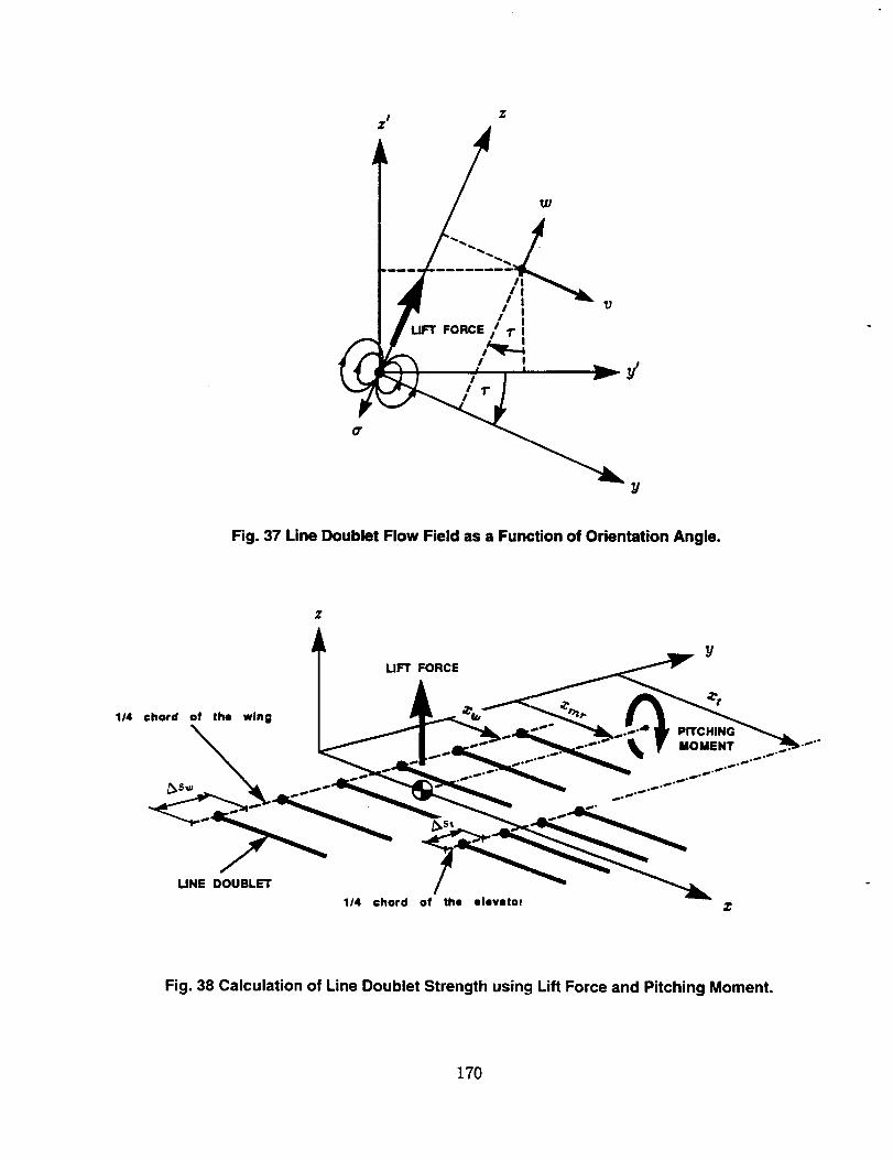
I I
I
Y
Fig. 37 Line Doublet Flow Field as a Function of Orientation Angle.
114 chord of the wing
LIFT FORCE
PITCHING
MOMENT
LINE DOUBLET
114 chord of the elevstor Z
Fig. 38 Calculation of Line Doublet Strength using Lift Force and Pitching Moment.
170
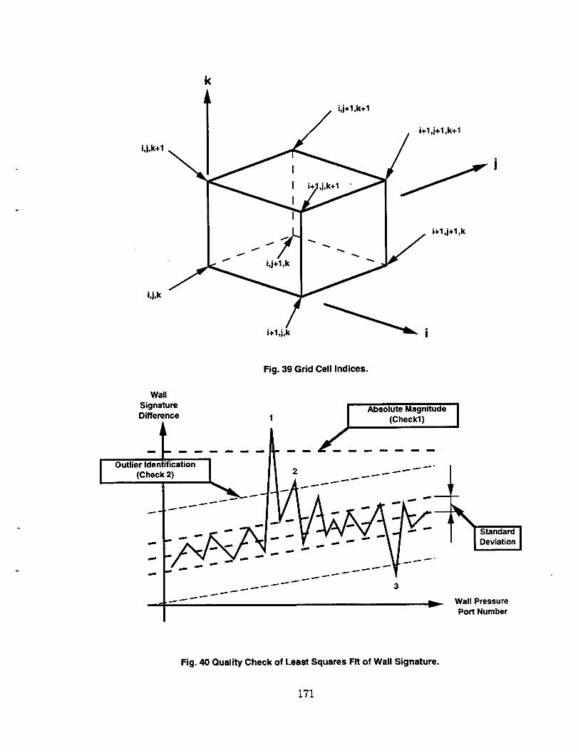
k
J_ i,j+l,k+l
i+l,j÷l,k+l
i,j,k+l
J
I
i÷l,j÷l ,k
Fig. 40 Quality Check of Least Squares Fit of Wall Signature.
171
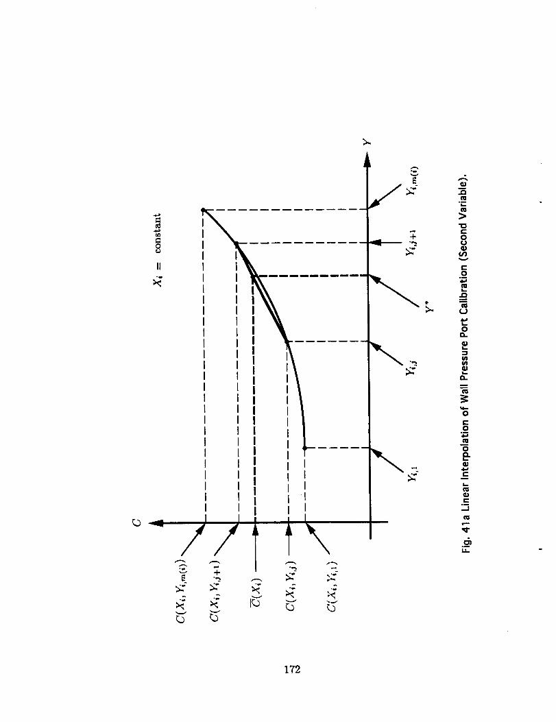
u
II
-/I I
!
.t:2
o_k_
"0c0u
Ul
r-0
°_4.0
L_
0
t_
0
e,-0
0
C
c
..1
i1
172
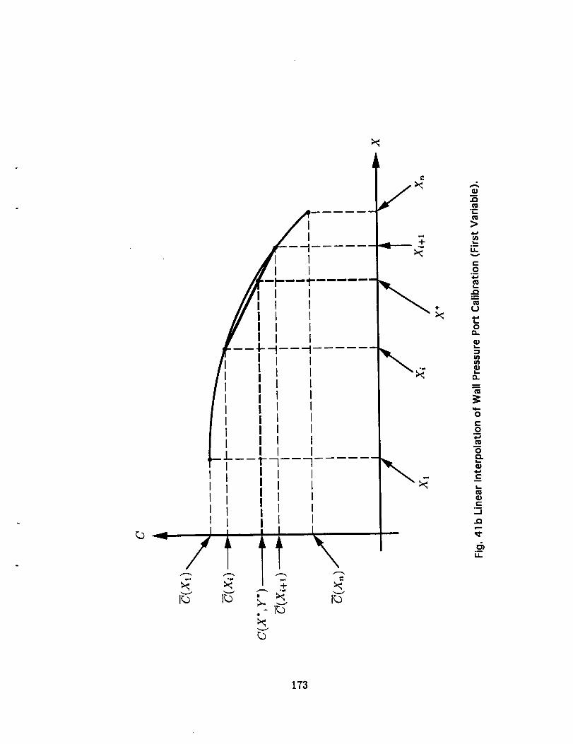
L
I
I I
III I I t
//I ', I "_I : I
/iIIIII
-4-
\
_p
..0
o_5=.
>
I.I_
¢.-
4-I
L_
t_0
a.
5,.
.=l0'}
a..
0
¢::04=_
C:)
4=,'¢.-
co_..J
¢....
IJ.
173
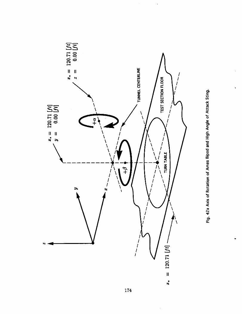
r.,-_q ira.,..1
II II
¢.==..-¢ m.._J
s===l
II II
\\
Q�\ I\ I\\\\
,\I \
II
v
\\
II
II
I!I
\ I\ I\ I
I \I \
I \I
c:4.J
t,n
(J(U
,<"6
o)e..
<cr,.
2::
"0I=
0
I:1.
r,nIn
E
0!-.2
o
0
o_X
.__
174
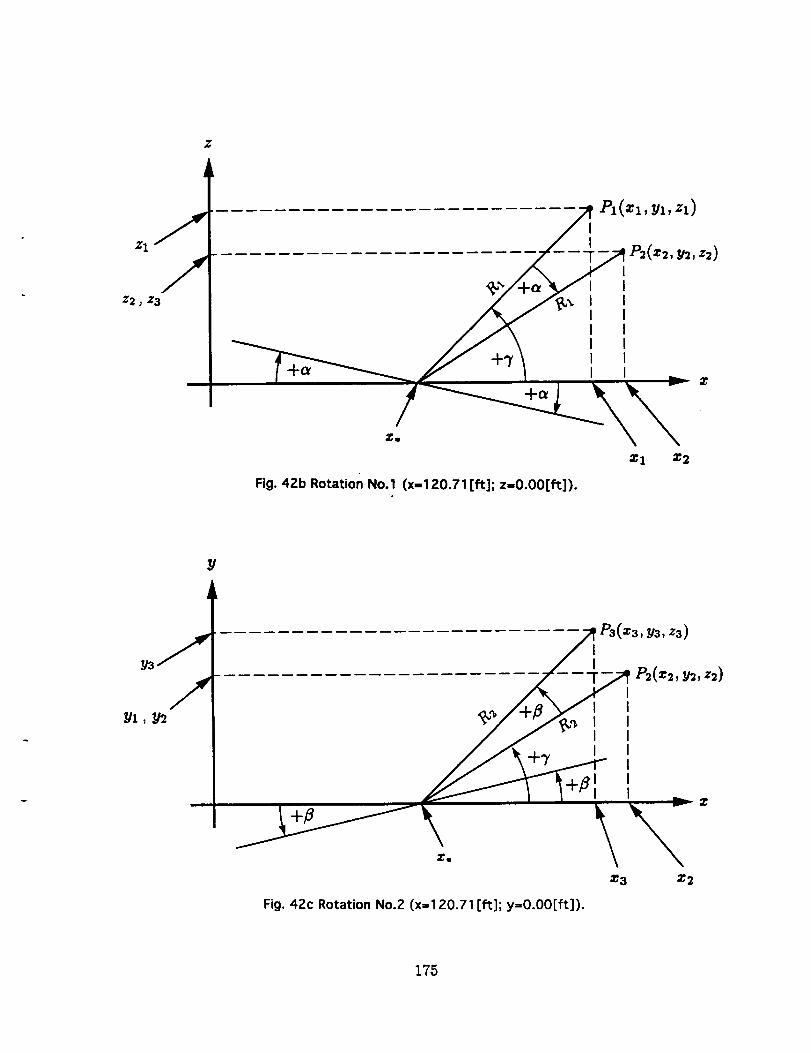
_/_- --'T-II I'P_(=_'_' _)
I I
Xl X2
Fig. 4Zb Rotation No.1 (x=120.71 [ft]; z=O.OO[ft])...
Y
P3(=3,y3,z3)
I I z
X3 X2
Fig. 42c Rotation No.Z (x=120.71 [ft]; y=O.OO[ft]).
175
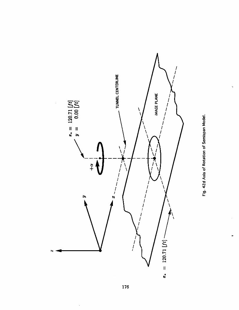
//
/#
\\
//
/
//
//
4
o
c_o
.mE
"6
o
0Ix
o
X
,<
LL
176
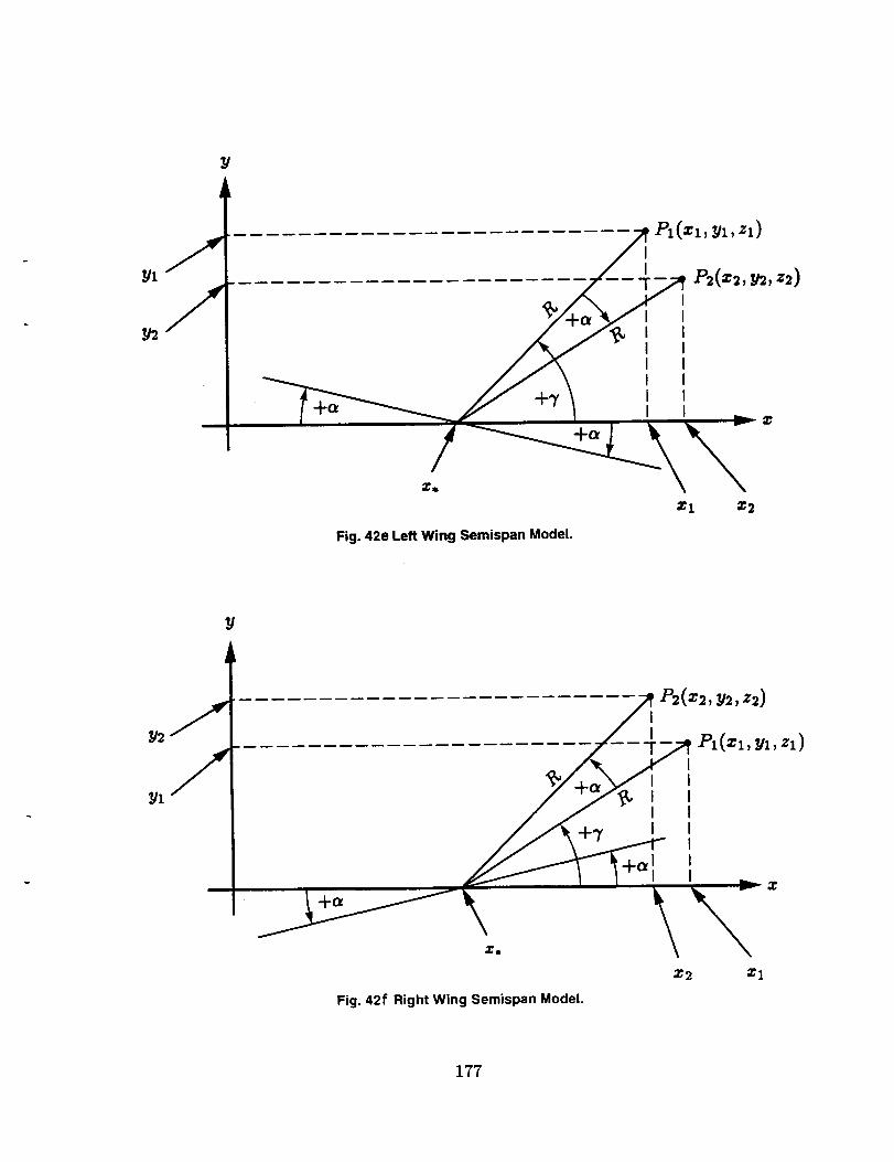
Y
_ Pl(zl,ul,zl)
Z
_1 :1:2
Fig. 42e Left Wing Semispan Model.
Y
Fig. 42t: Right Wing Semispan Model.
• 2 Z1
177
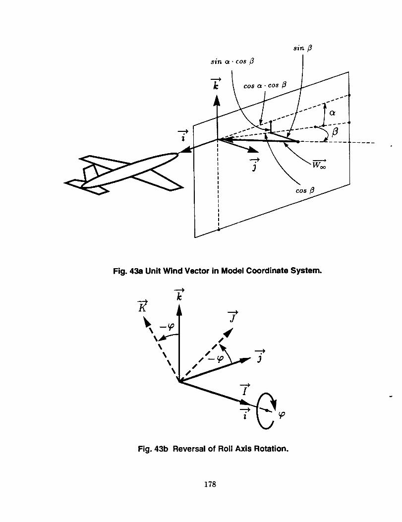
k
sin
cos
Fig. 43a Unit Wind Vector in Model Coordinate System.
k
J
/
Fig. 43b Reversal of Roll Axis Rotation.
178
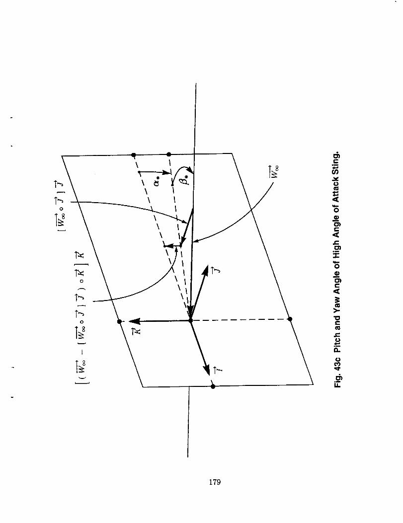
o
_ wA
\ I
\ I
I\\ I\ I
\\
\\
m_
0
0
0_C
e-
im
"l"qCB
0G_
m
e..
e-
11Dram
el
c_
6_IL
179
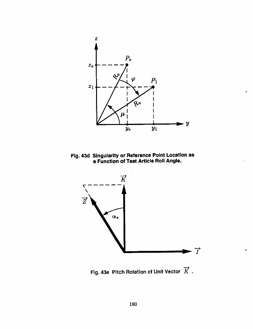
Yo Yl
Fig. 43d Singularity or Reference Point Location asa Function of Test Article Roll Angle.
K
I
Fig. 43e Pitch Rotation of Unit Vector K .
180
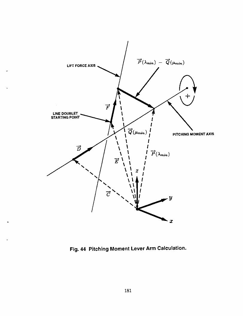
LIFT FORCE AXIS
I
UNE DOUBLET I
STARTING !
PITCHING MOMENT AXIS
Fig. 44 Pitching Moment Lever Arm Calculation.
181
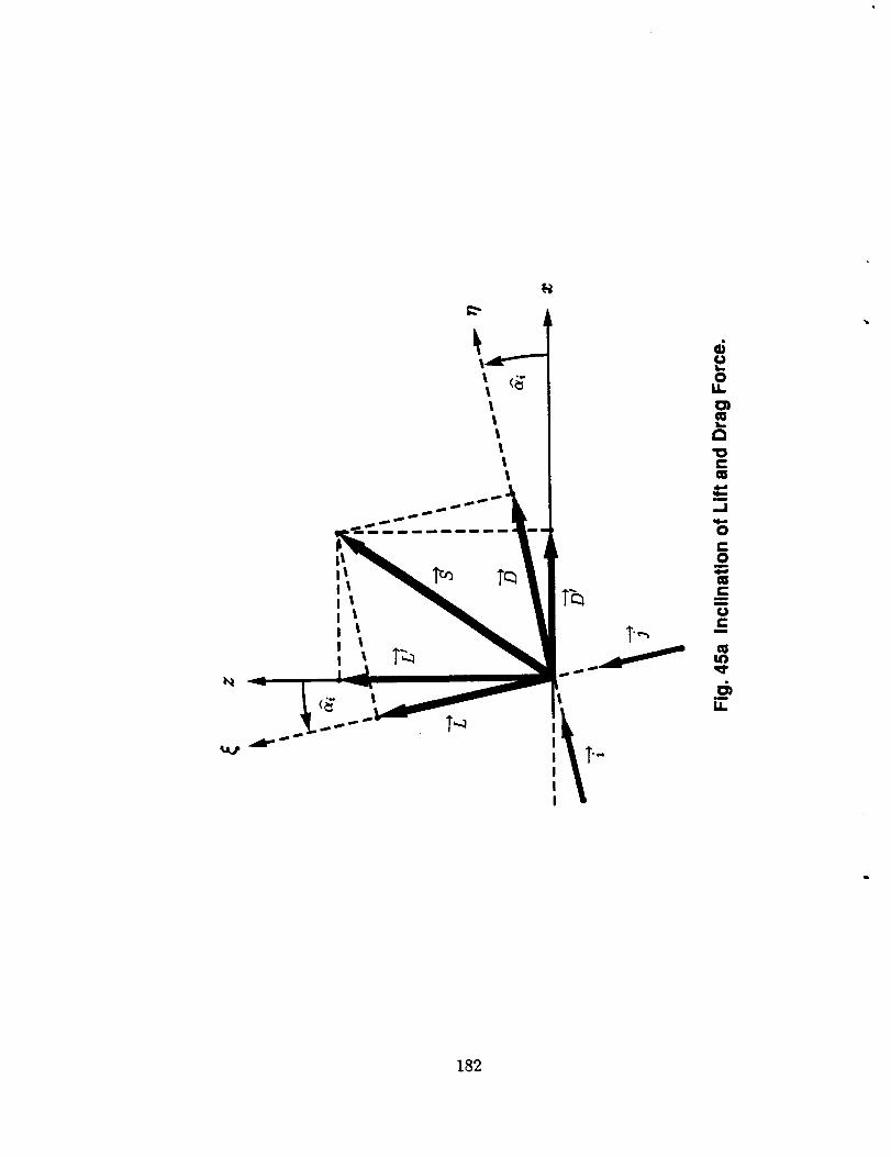
1llll1l
.._._._-_---]]]'_I lI lI lI lI lI lI lI
c.I1._
0U.
1__
"0Cw
bi
.4
0C:0
me-ra
m
r"m
m
I¢.
182
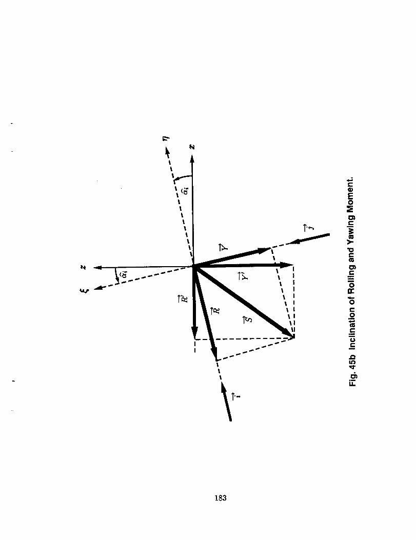
lI
lll
lllllllllII
C
EO
cm
c
mmm
Omr
O
Otm
mm
u
i
g_
183
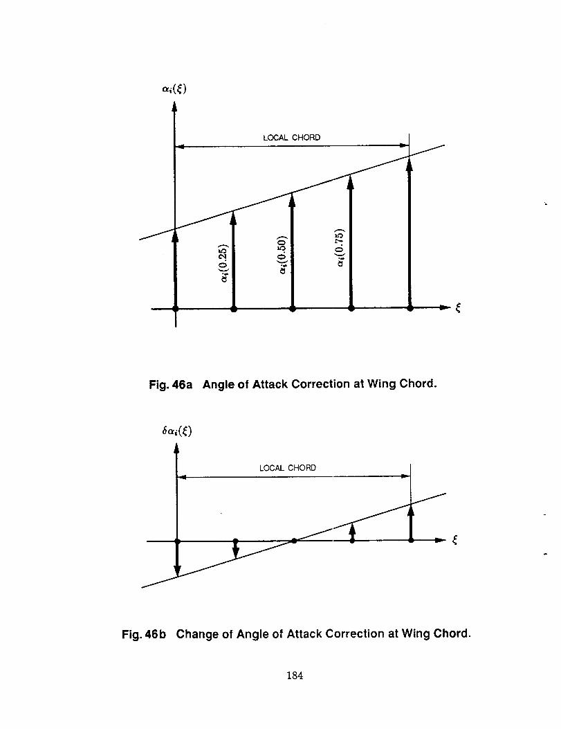
_(_)
LOCAL CHORD
Fig. 46a Angle of Attack Correction at Wing Chord.
LOCAL CHORD
J
Fig. 46b Change of Angle of Attack Correction at Wing Chord.
184
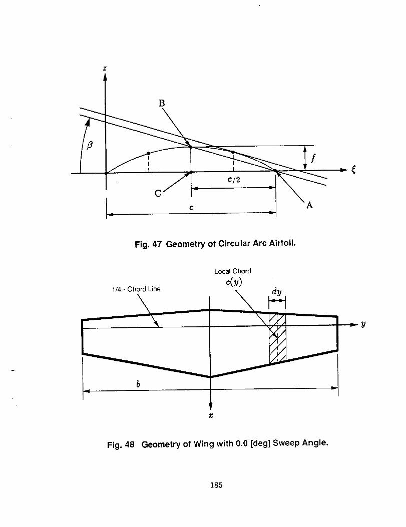
2;
T B
b _ o! A
Fig. 47 Geometry of Circular Arc Airfoil.
1/4 - Chord Line
Local Chord
c(_)
r
Y
Fig. 48 Geometry of Wing with 0.0 [deg] Sweep Angle.
185
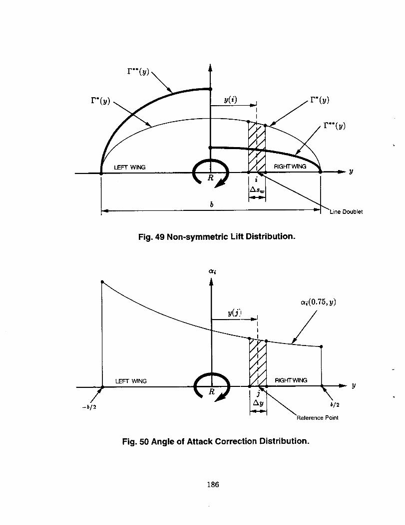
r'(v)
r"(v)
LEFT WING
R
v(;)
=, f r'(v)..
RIGHTW1NG "__ _ Y
v Line Doublet
Fig. 49 Non-symmetric Lilt Distribution.
LEFT WING
/-_/2
_(o.75,v)
Reference Point
Fig. 50 Angle of Attack Correction Distribution.
186
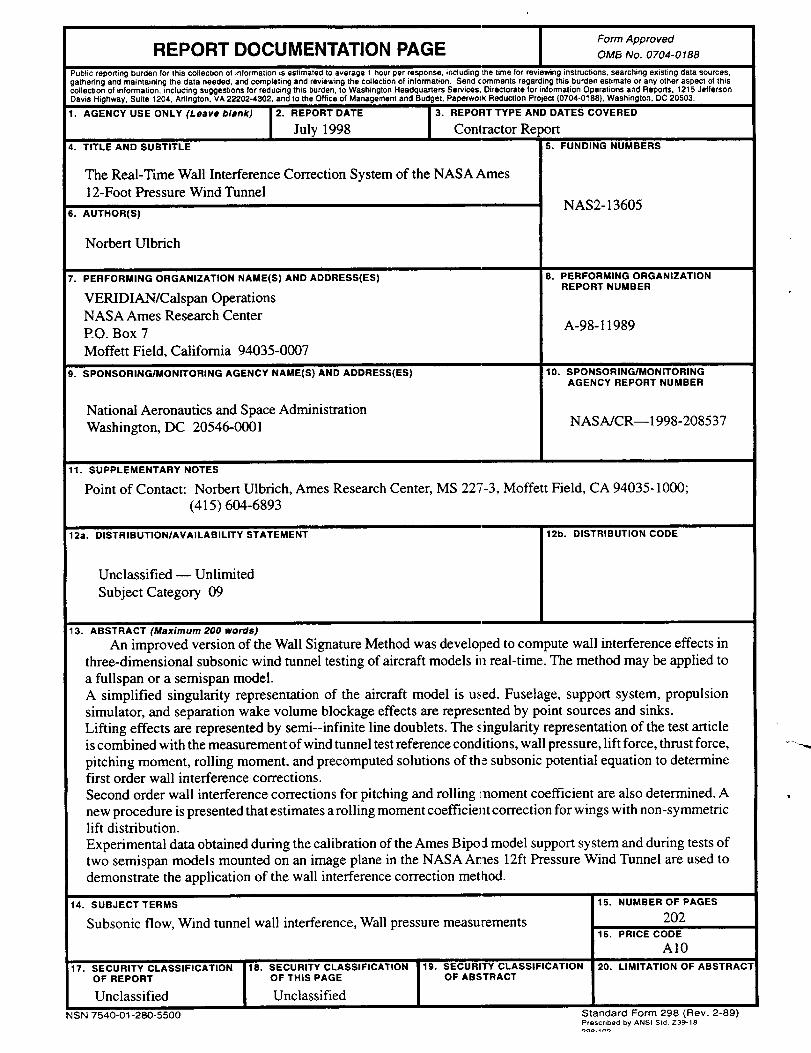
Form Approved
REPORT DOCUMENTATION PAGE No.ozo4-o18o
Public reporting burden for this collection of information is estimated to average 1 hour per response, including the time for reviewing instructions, searching existing data sources,gathering and maintaining the data needed, and completing and reviewing the collection of information. Send comments regarding this burden estimate or any other aspect of thiscollection of information, including suggestions for reducing this burden, to Washington Headquarters Services, Directorate for information Operations and Reports, 1215 JeffersonDavis Highway, Suite 1204, Arlington, VA 22202-4302, and to the Office of Management and Budget, Paperwo=_ Reduction Project (0704-0188). Washington, DC 20503.
i1. AGENCY USE ONLY (Leave blank) 2. REPORT DATE 3. REPORT TYPE AND DATES COVERED
July 1998 Contractor Report4. TITLE AND SUBTITLE 5. FUNDING NUMBERS
The Real-Time Wall Interference Correction System of the NASA Ames12-Foot Pressure Wind Tunnel
6. AUTHOR(S)
Norbert Ulbrich
7. PERFORMINGORGANIZATIONNAME(S)ANDADDRESS(ES)
VERIDIAN/Calspan OperationsNASA Ames Research Center
P.O. Box 7
Moffett Field, California 94035-0007
9. SPONSORING/MONITORINGAGENCYNAMEtS)ANDADDRESS(ES)
National Aeronautics and Space Administration
Washington, DC 20546-0001
NAS2-13605
8. PERFORMING ORGANIZATIONREPORT NUMBER
A-98-11989
10. SPONSORING/MONITORINGAGENCY REPORT NUMBER
NASA/CR--1998-208537
11. SUPPLEMENTARY NOTES
Point of Contact: Norbert Ulbrich, Ames Research Center, MS 227-3, Moffett Field, CA 94035-1000;
(415) 604-6893
12a. DISTRIBUTION/AVAILABILITY STATEMENT
Unclassified -- Unlimited
Subject Category 09
12b. DISTRIBUTION CODE
13. ABSTRACT (Maximum 200 Words)
An improved version of the Wall Signature Method was developed to compute wall interference effects inthree-dimensional subsonic wind tunnel testing of aircraft models i]1real-time. The method may be applied to
a fullspan or a semispan model.
A simplified singularity representation of the aircraft model is used. Fuselage, support system, propulsionsimulator, and separation wake volume blockage effects are represented by point sources and sinks.
Lifting effects are represented by semi--infinite line doublets. The singularity representation of the test articleis combined with the measurement of wind tunnel test reference conditions, wall pressure, lift force, thrust force,
pitching moment, rolling moment, and precomputed solutions of the subsonic potential equation to determinefirst order wall interference corrections.
Second order wall interference corrections for pitching and rolling _aaoment coefficient are also determined. A
new procedure is presented that estimates a rolling moment coefficient correction for wings with non-symmetriclift distribution.
Experimental data obtained during the calibration of the Ames Bipod model support system and during tests oftwo semispan models mounted on an image plane in the NASA Araes 12ft Pressure Wind Tunnel are used to
demonstrate the application of the wall interference correction method.
14. SUBJECT TERMS
Subsonic flow, Wind tunnel wall interference, Wall pressure measurements
17. SECURITY CLASSIFICATION 18. SECURITY CLASSIFICATIONOF REPORT OF THIS PAGE
Unclassified Unclassified
NSN 7540-01-280-5500
19. SECURITY CLASSIFICATIONOF ABSTRACT
15. NUMBER OF PAGES
20216. PRICE CODE
A10
20. LIMITATION OF ABSTRACT
Standard Form 298 (Rev. 2-89)Prescribed by ANSI Std. Z39-1e