The RBI’s Monetary Policy Reaction Function Does ... Bhattacharya_rev1_8Jan0… · The RBI’s Monetary Policy Reaction Function Does monetary policy in India follow an ... Section

The RBI’s Monetary Policy Reaction Function

Does monetary policy in India follow an inflation targeting rule?

Rituparna Banerjee

Saugata Bhattacharya*

Axis Bank Limited

January 2008

Revised Version

Paper submitted for the Annual Conference on Money & Finance, 2008, IGIDR

Abstract

The paper assesses the RBI’s monetary policy response function to economic conditions in India using limited dependent models. Given the non-uniform and discrete nature of intervention, these models are likely to provide a more appropriate framework of analysis than the linear “Taylor Rules” usually used. The main result of this paper is that the RBI’s monetary policy, since 2000, seems to have targeted the current output gap rather than inflation. There is evidence of greater persistence in the rate hike sequence than in the rate cut, which might be construed as indirect evidence of asymmetry in the response function. As possible explanation of the targeting of the output gap, we find that the current and lagged output gap does indeed affect inflation.

* E-mail address: [email protected]. Correspondence address: Saugata Bhattacharya, Risk Department, Axis Bank, Maker Towers F, 13th Floor, Cuffe Parade, Mumbai, 400 005, India.

The views expressed in the paper are personal and should not be attributed to the institution to which the authors are affiliated.

2

I. INTRODUCTION The statistical analysis of the determinants of monetary policy stance of central banks has

been mainly centred around the estimation of dynamic linear regression models in the

spirit of the so-called “Taylor Rules”. These rules characterize the appropriate optimal

policy reaction function of a central bank in terms of the adjustment of a short-term

interest rate under its control (see Taylor [1993, 1999]). Conventionally, adjustments in

the interest rate targets are related to inflation, output gaps exchange rate and foreign

interest rates in an open economy framework. For the most part, derivations of optimal

rules for the conduct of monetary policy have taken place in a linear-quadratic framework

arising out of a quadratic objective function for the central bank and a linear dynamic

system describing the economy. When the policy instrument is a short-term interest rate,

this combination results in a linear reaction function (Taylor Rule), whereby central

banks adjust nominal interest rates proportionately to inflation and output deviations from

their targets.

This approach, however, might be too restrictive when analyzing some distinctive

features that characterize a central bank’s intervention. The critique may be grouped into

two distinct features.

The first set of problems of the linear quadratic response functions relate to the nature of

the central bank interventions. First, the policy interest rate is changed irregularly,

sometimes as often as twice a month and at other times as seldom as once in two quarters.

Secondly, the changes are done in discrete adjustments, typically of 25 basis points,

rather than in a continuous fashion. The infrequent and discrete nature of interest rate

might render standard time series techniques inappropriate since they are devised to

model continuous data arriving at fixed intervals of time.

The second set relates to the nature of the inflation-output tradeoff itself. In the short

term, this trade-off might be non-linear. There is also a growing body of research that

indicates that central banks may have asymmetric preferences with respect to inflation

and / or output gaps. Some central banks, for instance, may have a greater aversion to

recessions than expansions. Others find that some central banks associate a larger loss to

3

positive rather than negative deviations of inflation, resulting in the inclusion of the

conditional variance of inflation as an additional argument in the Taylor rule.

There are a number of empirical studies in the literature which use variants of these

techniques. Dolado and Dolores (2002), Dolado et al. (2003) use Marked Point Processes

to investigate the actions of the Bank of Spain and other European central banks.

Gascoigne and Turner (2003) use simpler ordered probit models to look at the response

behaviour of the Bank of England. Our paper expands the scope of the latter in analyzing

the conduct of monetary policy in India.

This paper attempts to examine the validity of some of these issues in the Indian context.

Our approach in this paper is based upon the estimation of limited dependent models

(both Probit and Logit) to determine the probability of an intervention by the Reserve

Bank of India (RBI). Both binary and ordered representations are used. In general,

attempts to address these issues through a standard linear Taylor Rules approach is likely

to lead to misleading inferences.

The paper is organized as follows. Section II provides a brief overview of the RBI’s

evolving approach to monetary policy making and its views on transmission channels of

monetary policy actions. Section III details the methodologies that we have adopted in

the paper. Section IV explains our inferences and results of the models. Section V looks

at the empirical relation between inflation and the potential output gap in India. Section

VI concludes and indicates avenues for future research.

II. THE RBI’S APPROACH TO MONETARY POLICY From the mid-1980s until 1998, the RBI used a monetary-targeting framework focused

on interest rates, while at the same time monitoring developments in the real sector. Since

1998, it has widened the framework and begun to pursue a multiple-indicator approach.

The RBI’s Working Group on Money Supply (RBI, 1998) pointed out that monetary

policy exclusively based on money demand could lack precision. As a result while money

supply continued to serve as an important information variable, the RBI felt it necessary

to monitor a set of additional indicators for monetary policy formulation. Accordingly,

the RBI adopted a multiple indicator approach from 1998 wherein, besides monetary

4

aggregates, information pertaining to a range of rates of return in different financial

market segments along with the movements in currency, credit, the fiscal position,

merchandise trade, capital flows, the inflation rate, the exchange rate, refinancing and

transactions in foreign exchange – which are available on a high frequency basis – were

juxtaposed with data on output and the real sector activity for drawing policy

perspectives. Under this approach, the role of monetary aggregates as the exclusive

intermediate target have been de-emphasised and short-term policy interest rates have

gradually emerged as the operating target of monetary policy. Within the multiple goals

assigned to the monetary authority, the achievement of price and financial stability

received greater emphasis. This widening of the scope of variables monitored has partly

been enabled by the development of more sophisticated econometric models.

In this context, a recent paper (Kannan et al., 2006) provides valuable insights into the

current thinking at the central bank on monetary policy responses in India in an open

economy framework. It constructs a Monetary Conditions Index taking into account both

interest rate and exchange rate channels. Their results indicate that interest rates have

been more important than exchange rates in influencing monetary conditions in India.1

This Index is seen as supplementing the set of multiple indicators referred to above.

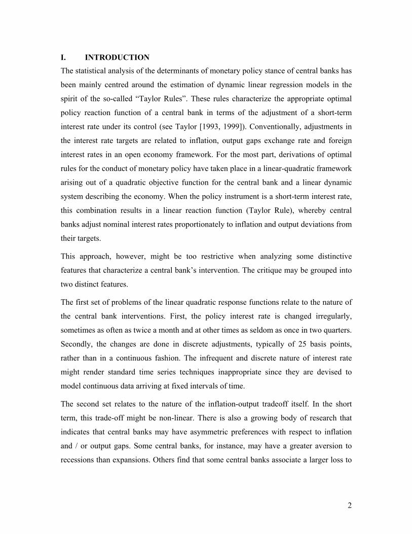
Chart 1 below depicts some of the monetary policy actions of the RBI during 2001to

2007 (till June), in the context of two of the more common variables included in “Taylor

Rules” approaches, viz., output and inflation. During this period, the RBI has lowered

CRR from 8.8% to 4.5% (in 6 steps) and then raised it to 7.5% (also in 6 steps, although

the last two were in August and October), The repo / reverse repo rate had been reduced 8

times (from 10% to 6%) and then raised 9 times (to 7.75%). The bank rate was reduced

thrice (to 6% in April ‘03) and then kept unchanged. It has used the three instruments

simultaneously only once (in November ’02) but has lately used a combination of the

CRR and repo rates. It has also occasionally used the repo – reverse repo corridor as an

instrument.

1 The authors have noted elsewhere that there is also a switching behaviour in the policy response between domestic interest rates and currency considerations, the most recent such episode being the middle of 2007, when the Rupee had appreciated sharply.

5

Chart 1: Timing and type of RBI monetary Policy actions

Notes: The lighter vertical lines indicate changes in repo, reverse repo and bank rates; darker vertical lines are CRR changes.

The easing phase of the RBI’s policy ended around the middle of 2003. The tightening

phase started in late 2004, patently designed to deal with rising inflation, couple with

what must have been perceived as unsustainably high industrial output growth. Casual

empiricism from the chart above indicates that that inflation was certainly restrained by

the policy tightening, but industrial output growth had become much more volatile.

II.a Issues and hypotheses

Given this background, the following issues are sought to be explored in the paper. The

ongoing statements from the RBI leave no doubt that they consider one or two of the list

of their multiple objectives to be of primary importance. For instance, liquidity

management has of late repeatedly been cited as one of the primary concerns of the RBI.

The primary target, in line with other central banks in the recent past has remained

inflation. So what then, is the primary strategy of the RBI? The paper attempts to

understand the process of targeting adopted by the RBI.

0M ar-01 Aug-01 Jan-02 Jun-02 Nov-02 Apr-03 Sep-03 Feb-04 Jul-04 Dec-04 M ay-05 Oct-05 M ar-06 Aug-06 Jan-07 Jun-07

0%

4%

8%

12%

16%RBI's policy change IIP grow th Inflation

Easing

Tightening

6

One of the assumptions of the paper is that there are two primary targets for monetary

policy: (i) inflation and (ii) an output gap.2 The other stated objectives are intermediate

targets. Is there any primacy in these two primary targets in the sense the RBI has given

undue weight to one, or are both equal in terms of their influence on the RBI’s policy

response. This issue is important since there is a significant corpus of research that seems

to indicate that many central banks target the current output gap. The logic is that this is

similar to targeting future inflation.

The second issue relates to the persistence of the responses. Given that an intervention

has happened, does the probability of another intervention change? Is there an asymmetry

in this persistence as well? Are the chances of a cut following a prior cut the same as

those of a hike following a prior hike?

A third issue is that of asymmetry in the monetary policy approach, with respect to the

phase of the business cycle. In other words, was the response behaviour different during a

downturn compared to that in an upswing?

III. MODELS AND METHODOLOGY

III.a Data

We have used monthly and quarterly data from June 2000 to August 2007 in our

regressions. We have used WPI inflation data since this is what the RBI declares as its

target. We have chosen the Index of Industrial Production (IIP) and GDP as our output

measures (for month and quarter periods, respectively) for the reasons specified below.

Our policy interest rate is the repo rate, since this has become the most operation policy

rate over the past few years.3 For quarterly data, the end quarter repo rate is taken as the

rate for that quarter. Quarterly inflation is the average rate over that quarter.

We have confined ourselves to the period post 2000 since our earlier work indicates

significant structural breaks during the late Nineties; these breaks are likely to have 2 This is a simplification of the dynamics of the response function. In India, exchange rate management is a significant response parameter, especially in the recent past. In 2007, there has been at least one episode where the RBI has shown a distinct “switching” behaviour in its response, with systematic and sustained intervention in the currency markets overriding inflation targeting. 3 The RBI has also used the width of the LAF repo and reverse repo corridor as a policy instrument, but the use has been more infrequent.

7

induced significant mis-specifications in our regressions. In addition, the RBI’s monetary

policy framework had changed significantly after the release of the Report of the

Working Group on monetary policy (op cited).

III.b Measurement of potential output

An important issue, especially in India, is the measurement of the output gap; unlike

developed countries, there are no official measures of potential output levels. Virmani

(2004) has earlier attempted an estimation of potential GDP, by comparing an

Unobserved Components model with an estimate derived from a Hodrick-Prescott (HP)

based smoothing. He found that sensitivities of the two models were not very different. In

other studies, estimates of the long run equilibrium level of output are found to be

sensitive to the method of estimation (see Mishkin (2007) for a recent overview and

references therein). We have used both monthly and quarterly measures of output, for

reasons explained below.

For the monthly exercise, the Index of Industrial Production (IIP) is a natural choice as

the output measure, for a variety of reasons. The most important was that would allow us

to model the monetary reactions on a monthly basis. Moreover, the IIP is a much more

homogenous measure of the Data Generation Process for economic activity. The

agriculture and allied products segments of the GDP are driven by many factors that are

relatively exogenous to the monetary policy stance. In addition, large segments of the

services sectors (transport, storage, communications, etc.) and construction are driven by

the industrial segment.

On the other hand, the quarterly GDP measure is a more comprehensive measure and is a

more natural fit to the quarterly reviews of monetary policy that is the RBI’s standard

practice.

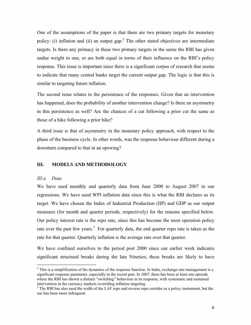
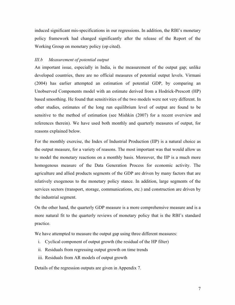
We have attempted to measure the output gap using three different measures:

i. Cyclical component of output growth (the residual of the HP filter)

ii. Residuals from regressing output growth on time trends

iii. Residuals from AR models of output growth

Details of the regression outputs are given in Appendix 7.

8

Chart 2a: Estimates of deviation of actual from potential industrial output in India

Chart 2b: Estimates of potential output gap using quarterly GDP for India

Notes: 1. The Resid_time series are the residuals obtained from regressing the growth rate

of the respective output measure on time (t = 1,2,3….). 2. Resid_AR are the residuals obtained from an AR representation of the growth rate

of the respective output measure. 3. HP_Cycle represents the cyclical component residual from the long term HP

filter.

-0.06

-0.04

-0.02

0.00

0.02

0.04

0.06

Jun-00

N o v-00

A pr-01

Sep-01

F eb-02

Jul-02

D ec-02

M ay-03

Oct-03

M ar-04

A ug-04

Jan-05

Jun-05

N o v-05

A pr-06

Sep-06

F eb-07

Jul-07

Resid_time Resid_AR Hpcycle

-5.0%

-2.5%

0.0%

2.5%

5.0%

2001Q1 2001Q4 2002Q3 2003Q2 2004Q1 2004Q4 2005Q3 2006Q2 2007Q1 2007Q4

GDPGR_Hpcycle GDPGR_RESID_AR GDPGR_RESID_TIME

9

Chart 2 above shows that the three measures of potential output seem to be congruent,

given the residuals are more or less of the same magnitude. In the rest of the paper, we

have used the HP-cycle method to measure the output gap4 using output growth.

III.c Limited Dependent Models

Prob (Repo_order) = F( Пt , Yt , Lagged_cut , Lagged_hike) …. (1)

where “Lagged_cut” and “Lagged_hike” are dummy variables, Пt is inflation, Yt is the

output measure.

The target variable “Repo_order” is a categorical variable constructed from the changes

in the repo rate. Given the unbalanced nature of the sample (zero changes occur more

frequently than either increases or cuts), we have used both Probit and Logit functional

forms to check for parameter instability and other mis-specifications.

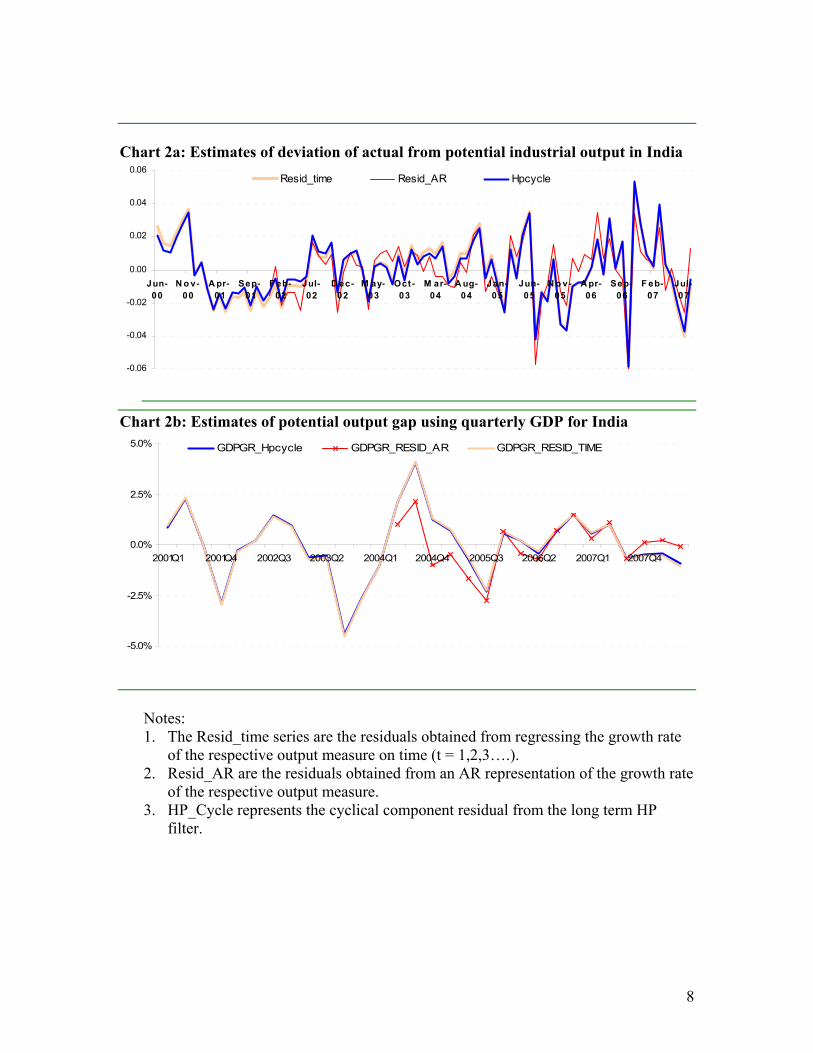
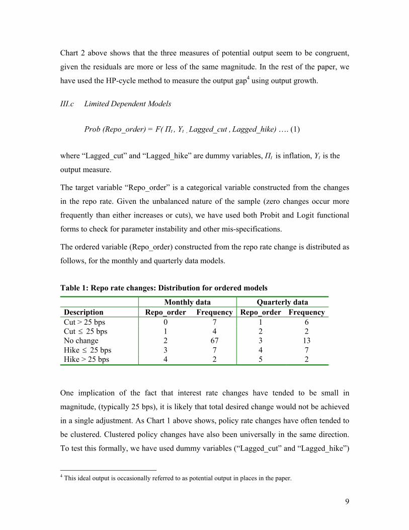
The ordered variable (Repo_order) constructed from the repo rate change is distributed as

follows, for the monthly and quarterly data models.

Table 1: Repo rate changes: Distribution for ordered models

Monthly data Quarterly data Description Repo_order Frequency Repo_order Frequency Cut > 25 bps 0 7 1 6 Cut ≤ 25 bps 1 4 2 2 No change 2 67 3 13 Hike ≤ 25 bps 3 7 4 7 Hike > 25 bps 4 2 5 2

One implication of the fact that interest rate changes have tended to be small in

magnitude, (typically 25 bps), it is likely that total desired change would not be achieved

in a single adjustment. As Chart 1 above shows, policy rate changes have often tended to

be clustered. Clustered policy changes have also been universally in the same direction.

To test this formally, we have used dummy variables (“Lagged_cut” and “Lagged_hike”)

4 This ideal output is occasionally referred to as potential output in places in the paper.

10

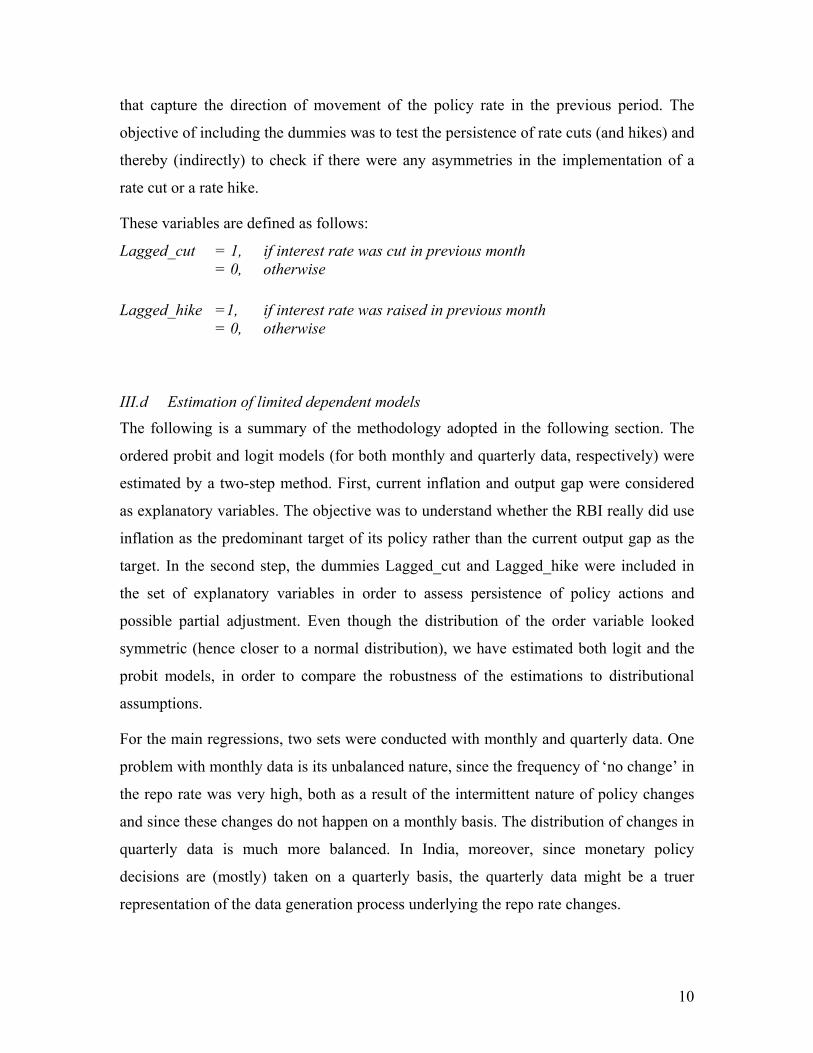
that capture the direction of movement of the policy rate in the previous period. The

objective of including the dummies was to test the persistence of rate cuts (and hikes) and

thereby (indirectly) to check if there were any asymmetries in the implementation of a

rate cut or a rate hike.

These variables are defined as follows:

Lagged_cut = 1, if interest rate was cut in previous month = 0, otherwise

Lagged_hike =1, if interest rate was raised in previous month = 0, otherwise III.d Estimation of limited dependent models

The following is a summary of the methodology adopted in the following section. The

ordered probit and logit models (for both monthly and quarterly data, respectively) were

estimated by a two-step method. First, current inflation and output gap were considered

as explanatory variables. The objective was to understand whether the RBI really did use

inflation as the predominant target of its policy rather than the current output gap as the

target. In the second step, the dummies Lagged_cut and Lagged_hike were included in

the set of explanatory variables in order to assess persistence of policy actions and

possible partial adjustment. Even though the distribution of the order variable looked

symmetric (hence closer to a normal distribution), we have estimated both logit and the

probit models, in order to compare the robustness of the estimations to distributional

assumptions.

For the main regressions, two sets were conducted with monthly and quarterly data. One

problem with monthly data is its unbalanced nature, since the frequency of ‘no change’ in

the repo rate was very high, both as a result of the intermittent nature of policy changes

and since these changes do not happen on a monthly basis. The distribution of changes in

quarterly data is much more balanced. In India, moreover, since monetary policy

decisions are (mostly) taken on a quarterly basis, the quarterly data might be a truer

representation of the data generation process underlying the repo rate changes.

11

A set of linear “Taylor Rules” type regressions are also finally reported to provide a basis

for comparison with the non-linear models, both to validate the results here and check

how many of the inferences turn out to be robust to the type of regression.

IV. RESULTS Details of the regression outputs for the specific models are given in Appendices 1

through 4. The following sections report the main inferences from the results. All

estimates were obtained using EViews 5.

IV.a Inferences with monthly data

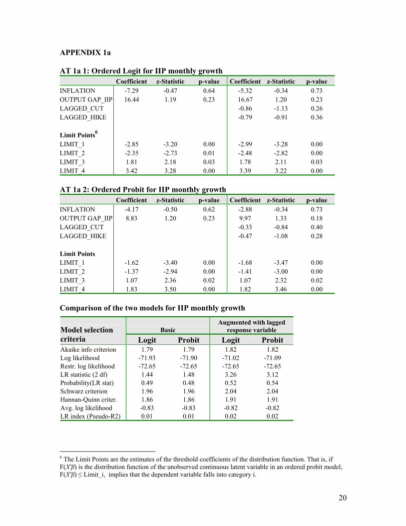
In the first stage, we estimated ordered regressions for interest rate changes in which the

explanatory variables were the current rate of inflation and the growth rate of adjusted

IIP. The outputs of the logit and the probit models are similar in terms of the model

selection criteria, with no particular reason to favour one over the other. The indicated

coefficients are also similar, although the strengths of the coefficients vary.

In both the logit and the probit models, the output gap was found to be more significant

than the current level of inflation. The contribution of the current rate of inflation in

determining the probability of interest rate changes is much smaller, as can be seen by the

low level of significance of this variable and the fact that its sign is opposite to that

expected. On the other hand, the output gap coefficient both has the correct sign and is

statistically more significant than the inflation coefficient.

The coefficients of the limits points (corresponding to the cut-off values of categories)

remain robust in sign and significance (and to an extent in magnitude) between the two

models and also to the inclusion of the lagged policy response dummies.

These lagged response dummies were added to check persistence of policy responses as

well as to capture possible inertia in policy responses. Although this behaviour is not well

understood in India as yet, it has been extensively studied for the US Federal Reserve. It

has been conjectured that the Fed’s tends to smooth changes in interest rates and adjust

12

its target for the Federal Funds Rate in a measured fashion. Such a reaction function,

generalizing the Taylor Rules, was studied by Clarida et al. (2000).

We have used a simplified version of their approach, by adding dummies for one-period

lagged cuts and hikes in a re-specified regression framework. After adding the lag

response dummies, the pseudo R2 improved from .01 to .02 in both the logit and probit

models. However, none of the dummies were significant. Recall that the “Lagged_cut”

dummy indicates the chance of a cut in interest rate given that there was a cut in the

previous month. “Lagged_hike” indicates the same for a hike.

The logit model performed marginally better than the probit according to the various

model selection criteria. Note that the inclusion of the lagged adjustment terms makes

little difference to the estimated coefficients for inflation and the output gap.

The results from our two functional forms were somewhat contradictory. In the logit

model, Lagged_cut dummy is more significant than the Lagged_hike dummy. On the

other hand, in the probit model, the Lagged_hike dummy was relatively stronger.

The high p-values of the coefficients in both the models suggest that there is no

statistically significant persistence in the monetary policy actions of the RBI.

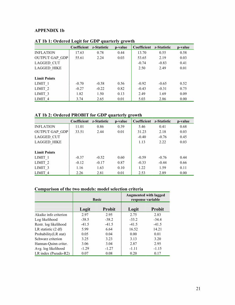
IV.b Inferences with quarterly data The unbalanced nature of the changes above is likely to have resulted in inefficient

estimation in the above equations. One way to correct for this distortion is to consider

monetary policy changes at quarterly intervals. The RBI, unlike many other central

banks, conducts a quarterly, rather than monthly, review of its monetary policy5. The

probability, therefore, of recording a change for any given quarter increases.

The following are some of the main differences and similarities with the model based on

monthly data. As with the models with monthly data, the output gap is always more

significant than inflation in both models.

The month-based logit and probit model showed different results for persistence effects,

while the results of the quarterly model were similar. For monthly data, Lagged_cut was

5 Although it has occasionally taken a mid-review monetary policy action.

13

more significant than Lagged_hike in the ordered logit model. On a quarterly time frame,

Lagged_hike dummy was more significant than Lagged_cut in both the models and the

results were also stronger. Overall, then, there is evidence of greater persistence of a rate

hike following another.

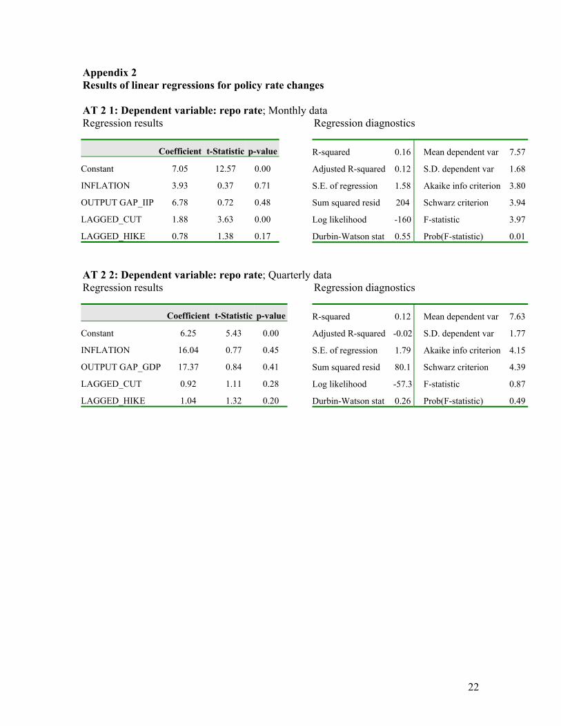
To understand the results of the logit regressions, we decided to benchmark them against

a linear “Taylor Rules” type of regression. The results of this regression are given in

Appendix 2. While the two regression results are not completely comparable, the overall

fit of the limited dependent regressions was slightly better than the linear model.

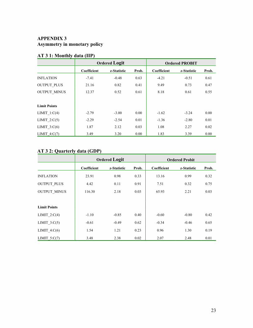
IV.c Asymmetry in monetary policy

In order to examine the existence of asymmetries in the monetary policy, the ordered

probit and logit models were re-specified. The output gap series was decomposed into

two parts: positive output gap (output_plus) and negative output gap (output_minus).

The results indicate relatively weak directionality in the response function. The monthly

data could not differentiate between the periods of positive and negative output gaps. The

quarterly data indicated a significant coefficient of the negative output gap variable,

which implies that the RBI is more likely to take policy action when output is below the

potential level than when it is above that level. However, the insignificant coefficients of

the limit points in the quarterly model suggest that the model is weak in categorizing the

estimated values, while the significant limit points in the monthly data indicated the

strength of the model. The results of these regressions are given in Appendix 3.

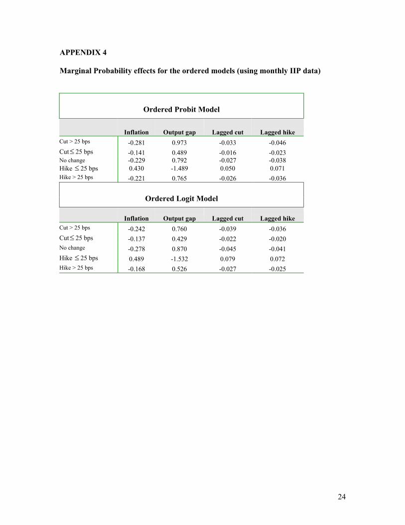
IV.d Marginal Effects

Marginal effects measure the change in predicted probability associated with changes in

the explanatory variables. The derived marginal probabilities from the ordered models are

given in Appendix 4. The marginal effects of output gap are found to be stronger than

inflation across all possible response categories. An increase in output gap raises the

probability of a larger response. Persistence effects are low and similar in both the

models, symmetric across cuts and hikes.

14

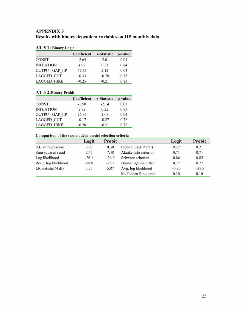
IV.e Limited Dependent models with binary dependent variables

Given the strong unbalanced classification in the ordered models, which might be causing

distortions in the estimated probabilities, we wished to substantiate the results of

symmetric responses of the RBI’s monetary policy. We investigate this further with a

simpler binary limited dependent model. Binary logit / probit models were estimated with

the binary repo rate indicators constructed as follows:

Repo_binary = 1, if the repo rate is hiked

= 0, if the repo rate is cut or unchanged

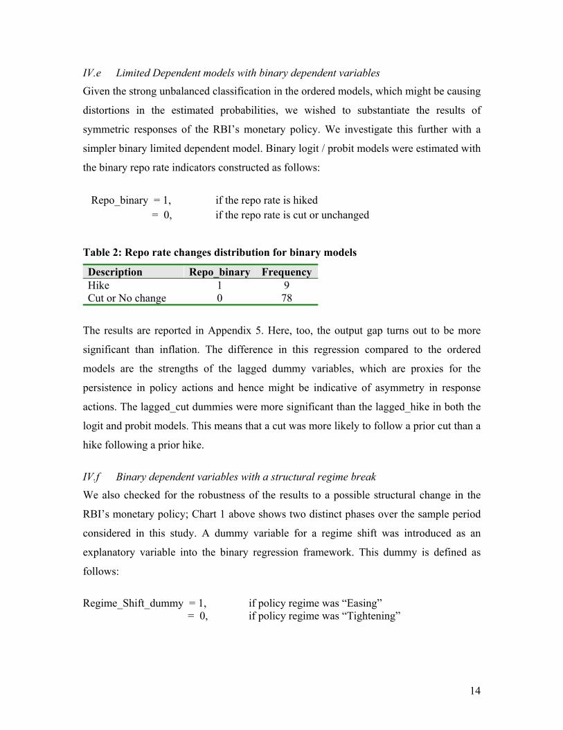
Table 2: Repo rate changes distribution for binary models

Description Repo_binary Frequency Hike 1 9 Cut or No change 0 78

The results are reported in Appendix 5. Here, too, the output gap turns out to be more

significant than inflation. The difference in this regression compared to the ordered

models are the strengths of the lagged dummy variables, which are proxies for the

persistence in policy actions and hence might be indicative of asymmetry in response

actions. The lagged_cut dummies were more significant than the lagged_hike in both the

logit and probit models. This means that a cut was more likely to follow a prior cut than a

hike following a prior hike.

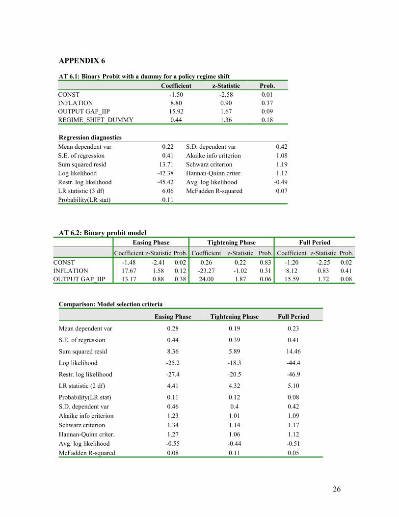
IV.f Binary dependent variables with a structural regime break

We also checked for the robustness of the results to a possible structural change in the

RBI’s monetary policy; Chart 1 above shows two distinct phases over the sample period

considered in this study. A dummy variable for a regime shift was introduced as an

explanatory variable into the binary regression framework. This dummy is defined as

follows:

Regime_Shift_dummy = 1, if policy regime was “Easing” = 0, if policy regime was “Tightening”

15

The corresponding probit regression for the full sample is as follows:

Prob (Repo_Change_binary) = F( Пt , Yt , Regime_Shift_dummy) …. (2)

Two other probit regressions were then done separately for the “Easing” and

“Tightening” phases of monetary policy (with the Regime Shift dummy obviously

deleted) to check for asymmetries in the policy regimes during these different regimes.

The binary dependent variable was re-specified as follows:

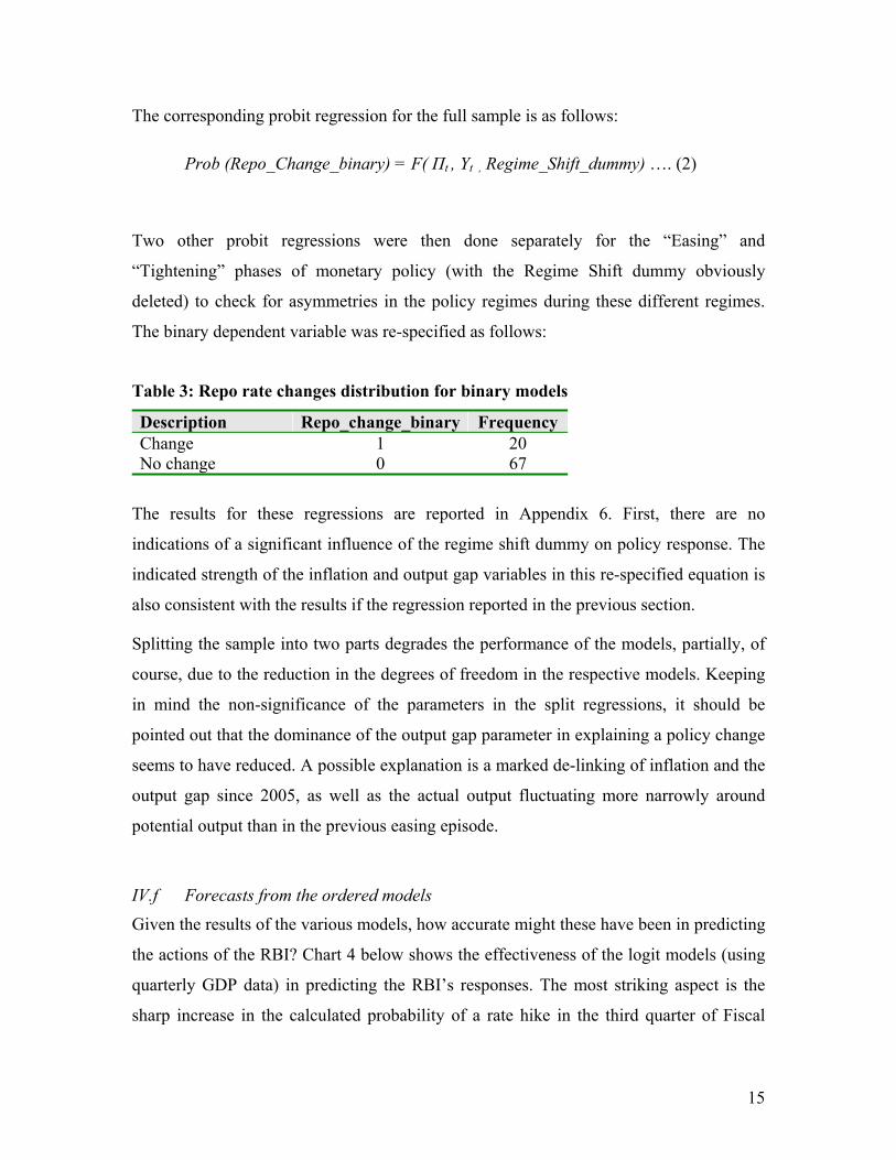
Table 3: Repo rate changes distribution for binary models

Description Repo_change_binary Frequency Change 1 20 No change 0 67

The results for these regressions are reported in Appendix 6. First, there are no

indications of a significant influence of the regime shift dummy on policy response. The

indicated strength of the inflation and output gap variables in this re-specified equation is

also consistent with the results if the regression reported in the previous section.

Splitting the sample into two parts degrades the performance of the models, partially, of

course, due to the reduction in the degrees of freedom in the respective models. Keeping

in mind the non-significance of the parameters in the split regressions, it should be

pointed out that the dominance of the output gap parameter in explaining a policy change

seems to have reduced. A possible explanation is a marked de-linking of inflation and the

output gap since 2005, as well as the actual output fluctuating more narrowly around

potential output than in the previous easing episode.

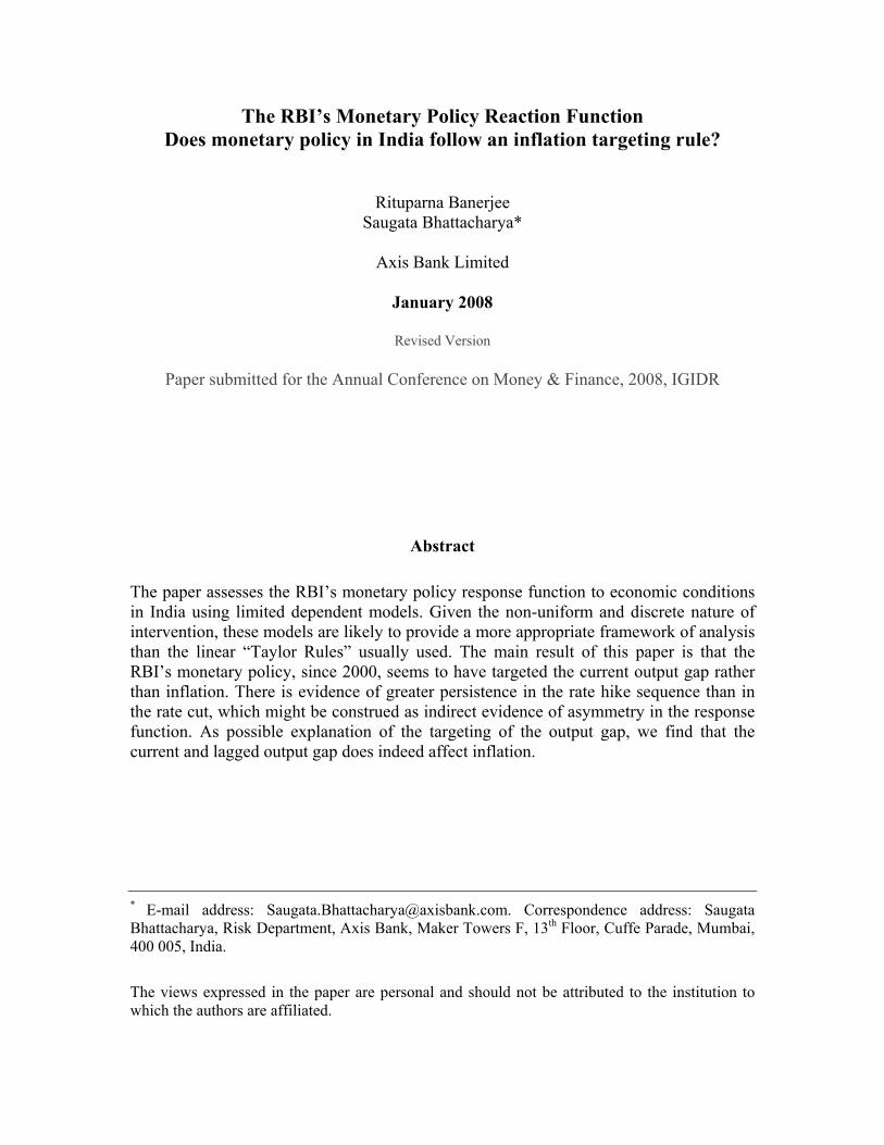
IV.f Forecasts from the ordered models

Given the results of the various models, how accurate might these have been in predicting

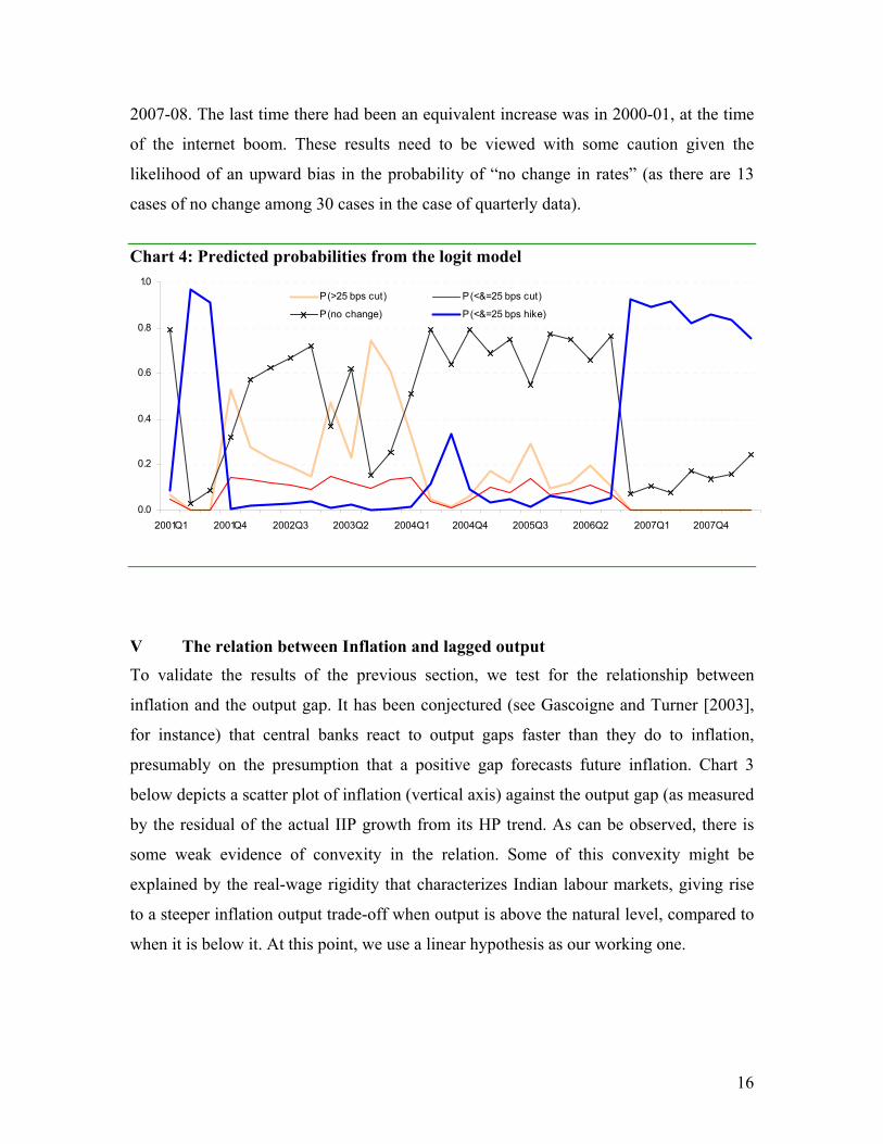
the actions of the RBI? Chart 4 below shows the effectiveness of the logit models (using

quarterly GDP data) in predicting the RBI’s responses. The most striking aspect is the

sharp increase in the calculated probability of a rate hike in the third quarter of Fiscal

16

2007-08. The last time there had been an equivalent increase was in 2000-01, at the time

of the internet boom. These results need to be viewed with some caution given the

likelihood of an upward bias in the probability of “no change in rates” (as there are 13

cases of no change among 30 cases in the case of quarterly data).

Chart 4: Predicted probabilities from the logit model

V The relation between Inflation and lagged output To validate the results of the previous section, we test for the relationship between

inflation and the output gap. It has been conjectured (see Gascoigne and Turner [2003],

for instance) that central banks react to output gaps faster than they do to inflation,

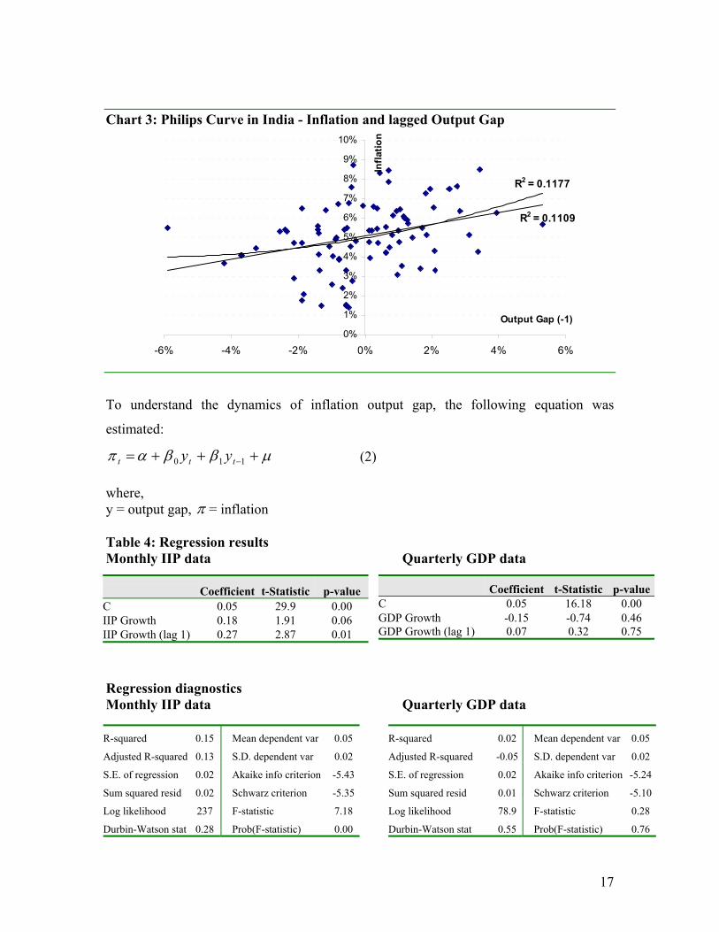
presumably on the presumption that a positive gap forecasts future inflation. Chart 3

below depicts a scatter plot of inflation (vertical axis) against the output gap (as measured

by the residual of the actual IIP growth from its HP trend. As can be observed, there is

some weak evidence of convexity in the relation. Some of this convexity might be

explained by the real-wage rigidity that characterizes Indian labour markets, giving rise

to a steeper inflation output trade-off when output is above the natural level, compared to

when it is below it. At this point, we use a linear hypothesis as our working one.

0.0

0.2

0.4

0.6

0.8

1.0

2001Q1 2001Q4 2002Q3 2003Q2 2004Q1 2004Q4 2005Q3 2006Q2 2007Q1 2007Q4

P(>25 bps cut) P(<&=25 bps cut)

P(no change) P(<&=25 bps hike)

17

Chart 3: Philips Curve in India - Inflation and lagged Output Gap

To understand the dynamics of inflation output gap, the following equation was

estimated:

µββαπ +++= −110 ttt yy (2) where, y = output gap, π = inflation Table 4: Regression results Monthly IIP data Quarterly GDP data Regression diagnostics Monthly IIP data Quarterly GDP data

R2 = 0.1109

R2 = 0.1177

0%

1%

2%

3%

4%

5%

6%

7%

8%

9%

10%

-6% -4% -2% 0% 2% 4% 6%

Output Gap (-1)

Infla

tion

Coefficient t-Statistic p-value C 0.05 29.9 0.00 IIP Growth 0.18 1.91 0.06 IIP Growth (lag 1) 0.27 2.87 0.01

Coefficient t-Statistic p-valueC 0.05 16.18 0.00 GDP Growth -0.15 -0.74 0.46 GDP Growth (lag 1) 0.07 0.32 0.75

R-squared 0.15 Mean dependent var 0.05

Adjusted R-squared 0.13 S.D. dependent var 0.02

S.E. of regression 0.02 Akaike info criterion -5.43

Sum squared resid 0.02 Schwarz criterion -5.35

Log likelihood 237 F-statistic 7.18

Durbin-Watson stat 0.28 Prob(F-statistic) 0.00


Adjusted R-squared -0.05 S.D. dependent var 0.02



Log likelihood 78.9 F-statistic 0.28


18

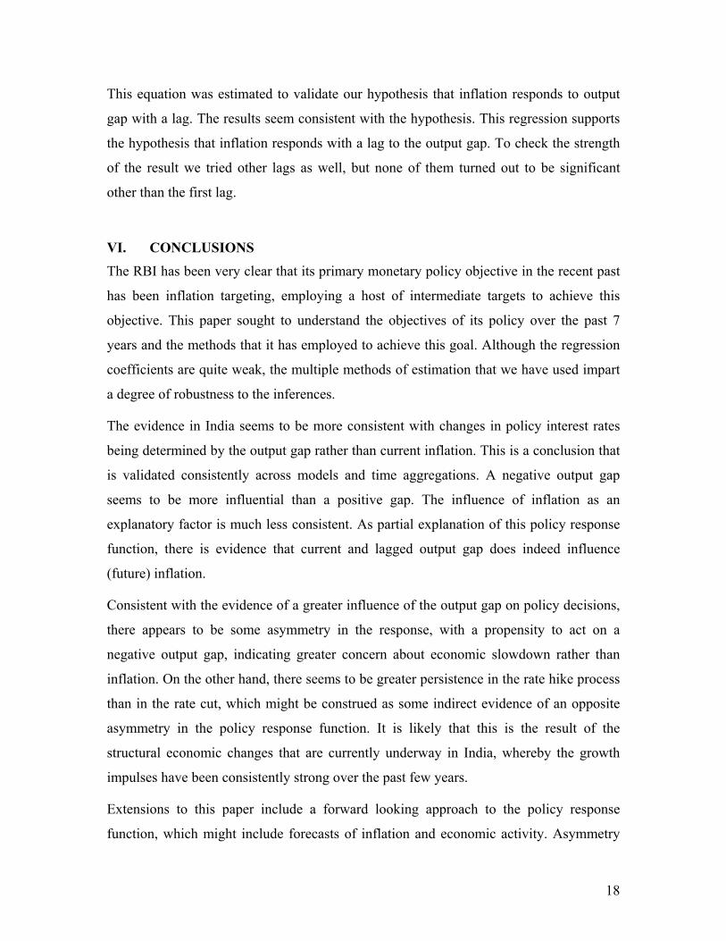
This equation was estimated to validate our hypothesis that inflation responds to output

gap with a lag. The results seem consistent with the hypothesis. This regression supports

the hypothesis that inflation responds with a lag to the output gap. To check the strength

of the result we tried other lags as well, but none of them turned out to be significant

other than the first lag.

VI. CONCLUSIONS The RBI has been very clear that its primary monetary policy objective in the recent past

has been inflation targeting, employing a host of intermediate targets to achieve this

objective. This paper sought to understand the objectives of its policy over the past 7

years and the methods that it has employed to achieve this goal. Although the regression

coefficients are quite weak, the multiple methods of estimation that we have used impart

a degree of robustness to the inferences.

The evidence in India seems to be more consistent with changes in policy interest rates

being determined by the output gap rather than current inflation. This is a conclusion that

is validated consistently across models and time aggregations. A negative output gap

seems to be more influential than a positive gap. The influence of inflation as an

explanatory factor is much less consistent. As partial explanation of this policy response

function, there is evidence that current and lagged output gap does indeed influence

(future) inflation.

Consistent with the evidence of a greater influence of the output gap on policy decisions,

there appears to be some asymmetry in the response, with a propensity to act on a

negative output gap, indicating greater concern about economic slowdown rather than

inflation. On the other hand, there seems to be greater persistence in the rate hike process

than in the rate cut, which might be construed as some indirect evidence of an opposite

asymmetry in the policy response function. It is likely that this is the result of the

structural economic changes that are currently underway in India, whereby the growth

impulses have been consistently strong over the past few years.

Extensions to this paper include a forward looking approach to the policy response

function, which might include forecasts of inflation and economic activity. Asymmetry

19

features need to be addressed in greater detail. The error dynamics of the limited

dependent class of models used here needs to be explored further. The regime switching

aspect of monetary policy also needs to be incorporated into the models.

REFERENCES

Clarida, R., Galf, J., and M. Gertler, 2000, "Monetary Policy Rules and Macroeconomic Stability: Evidence and Some Theory," Quarterly Journal of Economics vol. 115(1), pp. 147-180. Dolado, J. and R. Mario-Dolores, 2002, “Evaluating changes in the Bank of Spain’s interest rate target: an alternative approach using marked point processes”, Oxford Bulletin of Economics and Statistics, 64, 2, pp 159-182. Gascoigne, J. and P. Turner, 2003, “Asymmetries in Bank of England monetary policy”, Applied Economics Letters, vol. 11(10), pages 615-618, August; also Working Paper 007, Department of Economics, University of Sheffield. Kannan, R, S. Sanyal and B. B. Bhoi, 2006, “Monetary Conditions Index for India”, RBI Occasional Papers, vol 27(3), Winter. Mishkin, F. S., 2007, “Estimating potential output”, Speech at the Conference on Price Measurement for Monetary Policy, Federal Reserve Bank of Dallas, May 24. Mohan, Rakesh, 2006, “Monetary Policy Transmission in India”, paper presented at the Deputy Governor's Meeting on "Transmission Mechanisms for Monetary Policy in Emerging Market Economies - What is New?" at Bank for International Settlements, Basel on December 7-8 (and references therein). Reserve Bank of India, 1998, Report of the Working Group on Money Supply: Analytics and Methodology of Compilation (Chairman: Dr. Y.V. Reddy). Taylor, J., 1993, “Discretion versus policy rules in practice”, Carnegie – Rochester Conference on Public Policy, 39, pp. 195-214. Taylor, J., 1999, “The robustness and efficiency of monetary policy rules as guidelines for interest rate setting by the European Central Bank”, Journal of Monetary Economics, 43, pp. 655-679. Virmani, V., 2004, “Estimating output gap for the Indian economy”, IIM Ahmedabad Working Paper.

20

APPENDIX 1a AT 1a 1: Ordered Logit for IIP monthly growth Coefficient z-Statistic p-value Coefficient z-Statistic p-value INFLATION -7.29 -0.47 0.64 -5.32 -0.34 0.73 OUTPUT GAP_IIP 16.44 1.19 0.23 16.67 1.20 0.23 LAGGED_CUT -0.86 -1.13 0.26 LAGGED_HIKE -0.79 -0.91 0.36 Limit Points6 LIMIT_1 -2.85 -3.20 0.00 -2.99 -3.28 0.00 LIMIT_2 -2.35 -2.73 0.01 -2.48 -2.82 0.00 LIMIT_3 1.81 2.18 0.03 1.78 2.11 0.03 LIMIT_4 3.42 3.28 0.00 3.39 3.22 0.00 AT 1a 2: Ordered Probit for IIP monthly growth Coefficient z-Statistic p-value Coefficient z-Statistic p-value INFLATION -4.17 -0.50 0.62 -2.88 -0.34 0.73 OUTPUT GAP_IIP 8.83 1.20 0.23 9.97 1.33 0.18 LAGGED_CUT -0.33 -0.84 0.40 LAGGED_HIKE -0.47 -1.08 0.28 Limit Points LIMIT_1 -1.62 -3.40 0.00 -1.68 -3.47 0.00 LIMIT_2 -1.37 -2.94 0.00 -1.41 -3.00 0.00 LIMIT_3 1.07 2.36 0.02 1.07 2.32 0.02 LIMIT_4 1.83 3.50 0.00 1.82 3.46 0.00 Comparison of the two models for IIP monthly growth

Basic Augmented with lagged

response variable Model selection criteria Logit Probit Logit Probit Akaike info criterion 1.79 1.79 1.82 1.82 Log likelihood -71.93 -71.90 -71.02 -71.09 Restr. log likelihood -72.65 -72.65 -72.65 -72.65 LR statistic (2 df) 1.44 1.48 3.26 3.12 Probability(LR stat) 0.49 0.48 0.52 0.54 Schwarz criterion 1.96 1.96 2.04 2.04 Hannan-Quinn criter. 1.86 1.86 1.91 1.91 Avg. log likelihood -0.83 -0.83 -0.82 -0.82 LR index (Pseudo-R2) 0.01 0.01 0.02 0.02

6 The Limit Points are the estimates of the threshold coefficients of the distribution function. That is, if F(X'β) is the distribution function of the unobserved continuous latent variable in an ordered probit model, F(X'β) ≤ Limit_i, implies that the dependent variable falls into category i.

21

APPENDIX 1b AT 1b 1: Ordered Logit for GDP quarterly growth Coefficient z-Statistic p-value Coefficient z-Statistic p-value INFLATION 17.63 0.78 0.44 13.70 0.55 0.58 OUTPUT GAP_GDP 55.61 2.24 0.03 53.65 2.19 0.03 LAGGED_CUT -0.74 -0.83 0.41 LAGGED_HIKE 2.50 2.49 0.01 Limit Points LIMIT_1 -0.70 -0.58 0.56 -0.92 -0.65 0.52 LIMIT_2 -0.27 -0.22 0.82 -0.43 -0.31 0.75 LIMIT_3 1.82 1.50 0.13 2.49 1.69 0.09 LIMIT_4 3.74 2.65 0.01 5.03 2.86 0.00 AT 1b 2: Ordered PROBIT for GDP quarterly growth Coefficient z-Statistic p-value Coefficient z-Statistic p-value INFLATION 11.01 0.86 0.39 5.46 0.41 0.68 OUTPUT GAP_GDP 33.51 2.44 0.01 31.23 2.18 0.03 LAGGED_CUT -0.40 -0.76 0.45 LAGGED_HIKE 1.13 2.22 0.03 Limit Points LIMIT_1 -0.37 -0.52 0.60 -0.59 -0.76 0.44 LIMIT_2 -0.12 -0.17 0.87 -0.33 -0.44 0.66 LIMIT_3 1.16 1.63 0.10 1.22 1.59 0.11 LIMIT_4 2.26 2.81 0.01 2.53 2.89 0.00 Comparison of the two models: model selection criteria

Basic Augmented with lagged

response variable

Logit Probit Logit Probit Akaike info criterion 2.97 2.95 2.75 2.83 Log likelihood -38.5 -38.2 -33.2 -34.4 Restr. log likelihood -41.5 -41.5 -41.5 -41.5 LR statistic (2 df) 5.99 6.64 16.52 14.21 Probability(LR stat) 0.05 0.04 0.00 0.01 Schwarz criterion 3.25 3.23 3.13 3.20 Hannan-Quinn criter. 3.06 3.04 2.87 2.95 Avg. log likelihood -1.29 -1.27 -1.11 -1.15 LR index (Pseudo-R2) 0.07 0.08 0.20 0.17

22

Appendix 2 Results of linear regressions for policy rate changes AT 2 1: Dependent variable: repo rate; Monthly data Regression results Regression diagnostics AT 2 2: Dependent variable: repo rate; Quarterly data Regression results Regression diagnostics

Coefficient t-Statistic p-value

Constant 7.05 12.57 0.00

INFLATION 3.93 0.37 0.71

OUTPUT GAP_IIP 6.78 0.72 0.48

LAGGED_CUT 1.88 3.63 0.00

LAGGED_HIKE 0.78 1.38 0.17



S.E. of regression 1.58 Akaike info criterion 3.80

Sum squared resid 204 Schwarz criterion 3.94

Log likelihood -160 F-statistic 3.97


Coefficient t-Statistic p-value

Constant 6.25 5.43 0.00

INFLATION 16.04 0.77 0.45

OUTPUT GAP_GDP 17.37 0.84 0.41

LAGGED_CUT 0.92 1.11 0.28

LAGGED_HIKE 1.04 1.32 0.20


Adjusted R-squared -0.02 S.D. dependent var 1.77

S.E. of regression 1.79 Akaike info criterion 4.15

Sum squared resid 80.1 Schwarz criterion 4.39

Log likelihood -57.3 F-statistic 0.87


23

APPENDIX 3 Asymmetry in monetary policy AT 3 1: Monthly data (IIP) Ordered Logit Ordered PROBIT

Coefficient z-Statistic Prob. Coefficient z-Statistic Prob.

INFLATION -7.41 -0.48 0.63 -4.21 -0.51 0.61

OUTPUT_PLUS 21.16 0.82 0.41 9.49 0.73 0.47

OUTPUT_MINUS 12.37 0.52 0.61 8.18 0.61 0.55

Limit Points

LIMIT_1:C(4) -2.79 -3.00 0.00 -1.62 -3.24 0.00

LIMIT_2:C(5) -2.29 -2.54 0.01 -1.36 -2.80 0.01

LIMIT_3:C(6) 1.87 2.12 0.03 1.08 2.27 0.02

LIMIT_4:C(7) 3.49 3.20 0.00 1.83 3.39 0.00

AT 3 2: Quarterly data (GDP)

Ordered Logit Ordered Probit

Coefficient z-Statistic Prob. Coefficient z-Statistic Prob.

INFLATION 23.91 0.98 0.33 13.16 0.99 0.32

OUTPUT_PLUS 4.42 0.11 0.91 7.51 0.32 0.75

OUTPUT_MINUS 116.30 2.18 0.03 65.93 2.21 0.03

Limit Points

LIMIT_2:C(4) -1.10 -0.85 0.40 -0.60 -0.80 0.42

LIMIT_3:C(5) -0.61 -0.49 0.62 -0.34 -0.46 0.65

LIMIT_4:C(6) 1.54 1.21 0.23 0.96 1.30 0.19

LIMIT_5:C(7) 3.48 2.38 0.02 2.07 2.48 0.01

24

APPENDIX 4 Marginal Probability effects for the ordered models (using monthly IIP data)

Ordered Probit Model

Inflation Output gap Lagged cut Lagged hike Cut > 25 bps -0.281 0.973 -0.033 -0.046 Cut≤ 25 bps -0.141 0.489 -0.016 -0.023 No change -0.229 0.792 -0.027 -0.038 Hike ≤ 25 bps 0.430 -1.489 0.050 0.071 Hike > 25 bps -0.221 0.765 -0.026 -0.036

Ordered Logit Model

Inflation Output gap Lagged cut Lagged hike Cut > 25 bps -0.242 0.760 -0.039 -0.036 Cut≤ 25 bps -0.137 0.429 -0.022 -0.020 No change -0.278 0.870 -0.045 -0.041 Hike ≤ 25 bps 0.489 -1.532 0.079 0.072 Hike > 25 bps -0.168 0.526 -0.027 -0.025

25

APPENDIX 5 Results with binary dependent variables on IIP monthly data AT 5 1: Binary Logit

Coefficient z-Statistic p-valueCONST -2.64 -2.01 0.04 INFLATION 4.92 0.21 0.84 OUTPUT GAP_IIP 47.35 2.12 0.03 LAGGED_CUT -0.33 -0.28 0.78 LAGGED_HIKE -0.25 -0.21 0.83 AT 5 2:Binary Probit

Coefficient z-Statistic p-valueCONST -1.50 -2.14 0.03 INFLATION 2.82 0.22 0.83 OUTPUT GAP_IIP 25.85 2.08 0.04 LAGGED_CUT -0.17 -0.27 0.78 LAGGED_HIKE -0.20 -0.31 0.76 Comparison of the two models: model selection criteria Logit Probit Logit Probit S.E. of regression 0.30 0.30 Probability(LR stat) 0.22 0.21 Sum squared resid 7.45 7.48 Akaike info criterion 0.71 0.71 Log likelihood -26.1 -26.0 Schwarz criterion 0.86 0.85 Restr. log likelihood -28.9 -28.9 Hannan-Quinn criter. 0.77 0.77 LR statistic (4 df) 5.75 5.87 Avg. log likelihood -0.30 -0.30 McFadden R-squared 0.10 0.10

26

APPENDIX 6 AT 6.1: Binary Probit with a dummy for a policy regime shift

Coefficient z-Statistic Prob. CONST -1.50 -2.58 0.01 INFLATION 8.80 0.90 0.37 OUTPUT GAP_IIP 15.92 1.67 0.09 REGIME_SHIFT_DUMMY 0.44 1.36 0.18 Regression diagnostics Mean dependent var 0.22 S.D. dependent var 0.42 S.E. of regression 0.41 Akaike info criterion 1.08 Sum squared resid 13.71 Schwarz criterion 1.19 Log likelihood -42.38 Hannan-Quinn criter. 1.12 Restr. log likelihood -45.42 Avg. log likelihood -0.49 LR statistic (3 df) 6.06 McFadden R-squared 0.07 Probability(LR stat) 0.11 AT 6.2: Binary probit model

Easing Phase Tightening Phase Full Period Coefficient z-Statistic Prob. Coefficient z-Statistic Prob. Coefficient z-Statistic Prob.

CONST -1.48 -2.41 0.02 0.26 0.22 0.83 -1.20 -2.25 0.02INFLATION 17.67 1.58 0.12 -23.27 -1.02 0.31 8.12 0.83 0.41OUTPUT GAP_IIP 13.17 0.88 0.38 24.00 1.87 0.06 15.59 1.72 0.08

Comparison: Model selection criteria Easing Phase Tightening Phase Full Period

Mean dependent var 0.28 0.19 0.23

S.E. of regression 0.44 0.39 0.41

Sum squared resid 8.36 5.89 14.46

Log likelihood -25.2 -18.3 -44.4

Restr. log likelihood -27.4 -20.5 -46.9

LR statistic (2 df) 4.41 4.32 5.10

Probability(LR stat) 0.11 0.12 0.08 S.D. dependent var 0.46 0.4 0.42 Akaike info criterion 1.23 1.01 1.09 Schwarz criterion 1.34 1.14 1.17 Hannan-Quinn criter. 1.27 1.06 1.12 Avg. log likelihood -0.55 -0.44 -0.51 McFadden R-squared 0.08 0.11 0.05

27

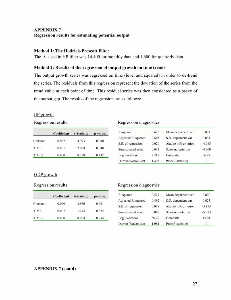
APPENDIX 7 Regression results for estimating potential output Method 1: The Hodrick-Prescott Filter The λ used in HP filter was 14,400 for monthly data and 1,600 for quarterly data. Method 2: Results of the regression of output growth on time trends

The output growth series was regressed on time (level and squared) in order to de-trend

the series. The residuals from this regression represent the deviation of the series from the

trend value at each point of time. This residual series was then considered as a proxy of

the output gap. The results of the regression are as follows:

IIP growth

Regression results Regression diagnostics GDP growth Regression results Regression diagnostics

APPENDIX 7 (contd)

Coefficient t-Statistic p-value.

Constant 0.032 4.993 0.000

TIME 0.001 2.089 0.040

TIME2 0.000 0.790 0.432






Durbin-Watson stat 1.495 Prob(F-statistic) 0

Coefficient t-Statistic p-value.

Constant 0.040 3.850 0.001

TIME 0.002 1.245 0.224

TIME2 0.000 0.084 0.934







28

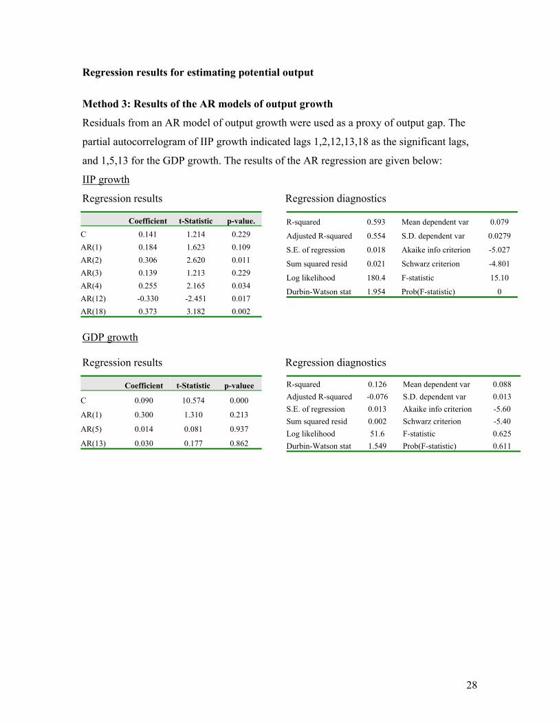
Regression results for estimating potential output

Method 3: Results of the AR models of output growth

Residuals from an AR model of output growth were used as a proxy of output gap. The

partial autocorrelogram of IIP growth indicated lags 1,2,12,13,18 as the significant lags,

and 1,5,13 for the GDP growth. The results of the AR regression are given below:

IIP growth

Regression results Regression diagnostics GDP growth Regression results Regression diagnostics

Coefficient t-Statistic p-value. C 0.141 1.214 0.229 AR(1) 0.184 1.623 0.109 AR(2) 0.306 2.620 0.011 AR(3) 0.139 1.213 0.229 AR(4) 0.255 2.165 0.034 AR(12) -0.330 -2.451 0.017 AR(18) 0.373 3.182 0.002







Coefficient t-Statistic p-valuee

C 0.090 10.574 0.000

AR(1) 0.300 1.310 0.213

AR(5) 0.014 0.081 0.937

AR(13) 0.030 0.177 0.862

R-squared 0.126 Mean dependent var 0.088 Adjusted R-squared -0.076 S.D. dependent var 0.013 S.E. of regression 0.013 Akaike info criterion -5.60 Sum squared resid 0.002 Schwarz criterion -5.40 Log likelihood 51.6 F-statistic 0.625 Durbin-Watson stat 1.549 Prob(F-statistic) 0.611

Documents

The RBI’s Monetary Policy Reaction Function Does ... Bhattacharya_rev1_8Jan0… · The RBI’s Monetary Policy Reaction Function Does monetary policy in India follow an ... Section