The Rayleigh−Ritz Methodfor Structural Analysis

Sinniah IlankoLuis E. Monterrubio

with assistance fromYusuke Mochida

MECHANICAL ENGINEERING AND SOLID MECHANICS SERIES

The Rayleigh−Ritz Method for Structural Analysis

To my late parents Saraswathyppillai and Sinniah, my late brother Senthinathan who encouraged and supported me during my studies at Manchester, my brothers Kumarabharathy, Kathirgamanathan, sister Sooriyakumari, my wife Krshnanandi, daughters Kavitha and Tehnuka, my in-laws, nephews, nieces, my supervisors Emeritus Professor Dickinson, the late Dr Tillman, my teachers from my old schools in Sri Lanka (Veemankamam Mahavithiyalaym, Mahajana College, Tellippalai), and all my lecturers and students, and colleagues both current and past.

Sinniah Ilanko

To my wife and son.

Luis Monterrubio

Series Editor Noël Challamel

The Rayleigh−Ritz Method for Structural Analysis

Sinniah Ilanko Luis E. Monterrubio with editorial assistance from

Yusuke Mochida

First published 2014 in Great Britain and the United States by ISTE Ltd and John Wiley & Sons, Inc.

Apart from any fair dealing for the purposes of research or private study, or criticism or review, as permitted under the Copyright, Designs and Patents Act 1988, this publication may only be reproduced, stored or transmitted, in any form or by any means, with the prior permission in writing of the publishers, or in the case of reprographic reproduction in accordance with the terms and licenses issued by the CLA. Enquiries concerning reproduction outside these terms should be sent to the publishers at the undermentioned address:

ISTE Ltd John Wiley & Sons, Inc. 27-37 St George’s Road 111 River Street London SW19 4EU Hoboken, NJ 07030 UK USA

www.iste.co.uk www.wiley.com

© ISTE Ltd 2014 The rights of Sinniah Ilanko and Luis E. Monterrubio to be identified as the authors of this work have been asserted by them in accordance with the Copyright, Designs and Patents Act 1988.

Library of Congress Control Number: 2014953191 British Library Cataloguing-in-Publication Data A CIP record for this book is available from the British Library ISBN 978-1-84821-638-9

Contents

PREFACE . . . . . . . . . . . . . . . . . . . . . . . . . . . . . . . . . . . . . . . . . . xi

INTRODUCTION AND HISTORICAL NOTES . . . . . . . . . . . . . . . . . . . . . . xiii

CHAPTER 1. PRINCIPLE OF CONSERVATION OF ENERGY AND RAYLEIGH’S PRINCIPLE . . . . . . . . . . . . . . . . . . . . . . . . 1

1.1. A simple pendulum . . . . . . . . . . . . . . . . . . . . . . . . . . . . . . . 1 1.2. A spring-mass system . . . . . . . . . . . . . . . . . . . . . . . . . . . . . . 4 1.3. A two degree of freedom system . . . . . . . . . . . . . . . . . . . . . . . 5

CHAPTER 2. RAYLEIGH’S PRINCIPLE AND ITS IMPLICATIONS . . . . . . . . . . . . . . . . . . . . . . . . . . . . . . . . . . . . 11

2.1. Rayleigh’s principle . . . . . . . . . . . . . . . . . . . . . . . . . . . . . . . 11 2.2. Proof . . . . . . . . . . . . . . . . . . . . . . . . . . . . . . . . . . . . . . . . 12 2.3. Example: a simply supported beam . . . . . . . . . . . . . . . . . . . . . . 13 2.4. Admissible functions: examples . . . . . . . . . . . . . . . . . . . . . . . . 15

CHAPTER 3. THE RAYLEIGH–RITZ METHOD AND SIMPLE APPLICATIONS . . . . . . . . . . . . . . . . . . . . . . . . . . . . . . 21

3.1. The Rayleigh–Ritz method . . . . . . . . . . . . . . . . . . . . . . . . . . . 21 3.2. Application of the Rayleigh–Ritz method . . . . . . . . . . . . . . . . . . 23

CHAPTER 4. LAGRANGIAN MULTIPLIER METHOD . . . . . . . . . . . . . . . . . 33

4.1. Handling constraints . . . . . . . . . . . . . . . . . . . . . . . . . . . . . . 33 4.2. Application to vibration of a constrained cantilever . . . . . . . . . . . . . . . . . . . . . . . . . . . . . . . . 33

vi The Rayleigh–Ritz Method for Structural Analysis

CHAPTER 5. COURANT’S PENALTY METHOD INCLUDING NEGATIVE STIFFNESS AND MASS TERMS . . . . . . . . . . . . . . . 39

5.1. Background . . . . . . . . . . . . . . . . . . . . . . . . . . . . . . . . . . . . 39 5.2. Penalty method for vibration analysis . . . . . . . . . . . . . . . . . . . . 40 5.3. Penalty method with negative stiffness . . . . . . . . . . . . . . . . . . . 43 5.4. Inertial penalty and eigenpenalty methods . . . . . . . . . . . . . . . . . 47 5.5. The bipenalty method . . . . . . . . . . . . . . . . . . . . . . . . . . . . . . 51

CHAPTER 6. SOME USEFUL MATHEMATICAL DERIVATIONS AND APPLICATIONS . . . . . . . . . . . . . . . . . . . . . . . . . . 55

6.1. Derivation of stiffness and mass matrix terms . . . . . . . . . . . . . . . 55 6.2. Frequently used potential and kinetic energy terms . . . . . . . . . . . . 57 6.3. Rigid body connected to a beam . . . . . . . . . . . . . . . . . . . . . . . 59 6.4. Finding the critical loads of a beam . . . . . . . . . . . . . . . . . . . . . 60

CHAPTER 7. THE THEOREM OF SEPARATION AND ASYMPTOTIC MODELING THEOREMS . . . . . . . . . . . . . . . . . . . . . 67

7.1. Rayleigh’s theorem of separation and the basis of the Ritz method . . . . . . . . . . . . . . . . . . . . . . . . . . . . . 67 7.2. Proof of convergence in asymptotic modeling . . . . . . . . . . . . . . . 71

7.2.1. The natural frequencies of an n DOF system with one additional positive or negative restraint . . . . . . . . . . . . . . . . . . . . . . . . . . . . . . . . . . 72 7.2.2. The natural frequencies of an n DOF system with h additional positive or negative restraints . . . . . . . . . . . . . . . . . . . . . . . . . . . . . . . . 79

7.3. Applicability of theorems (1) and (2) for continuous systems . . . . . . . . . . . . . . . . . . . . . . . . . . . . . . 80

CHAPTER 8. ADMISSIBLE FUNCTIONS . . . . . . . . . . . . . . . . . . . . . . . . 81

8.1. Choosing the best functions . . . . . . . . . . . . . . . . . . . . . . . . . . 81 8.2. Strategy for choosing the functions . . . . . . . . . . . . . . . . . . . . . . 82 8.3. Admissible functions for an Euler–Bernoulli beam . . . . . . . . . . . . . . . . . . . . . . . . . . . . . . . . 83 8.4. Proof of convergence . . . . . . . . . . . . . . . . . . . . . . . . . . . . . . 86

CHAPTER 9. NATURAL FREQUENCIES AND MODES OF BEAMS . . . . . . . . . . . . . . . . . . . . . . . . . . . . . . . . . 89

9.1. Introduction . . . . . . . . . . . . . . . . . . . . . . . . . . . . . . . . . . . . 89

Contents vii

9.2. Theoretical derivations of the eigenvalue problems . . . . . . . . . . . . . . . . . . . . . . . . . . . . . . . . . 89 9.3. Derivation of the eigenvalue problem for beams . . . . . . . . . . . . . . . . . . . . . . . . . . . . . . . . . . . . . . . . 91 9.4. Building the stiffness, mass matrices and penalty matrices . . . . . . . . . . . . . . . . . . . . . . . . . . . . . . . . . 94

9.4.1. Terms of the non-dimensional stiffness matrix . . . . . . . . . . . . . . . . . . . . . . . . . . . . . . . . . 95 9.4.2. Terms of the non-dimensional mass matrix . . . . . . . . . . . . . . . . . . . . . . . . . . . . . . . . . . 98 9.4.3. Terms of the non-dimensional penalty matrix . . . . . . . . . . . . . . . . . . . . . . . . . . . . . . . . . . 101

9.5. Modes of vibration . . . . . . . . . . . . . . . . . . . . . . . . . . . . . . . 103 9.6. Results . . . . . . . . . . . . . . . . . . . . . . . . . . . . . . . . . . . . . . . 104

9.6.1. Free–free beam . . . . . . . . . . . . . . . . . . . . . . . . . . . . . . . 104 9.6.2. Clamped–clamped beam using 250 terms . . . . . . . . . . . . . . . 105 9.6.3. Beam with classical and sliding boundary conditions using inertial restraints to model constraints at the edges of the beam . . . . . . . . . . . . . . . . . 108

9.7. Modes of vibration . . . . . . . . . . . . . . . . . . . . . . . . . . . . . . . 111

CHAPTER 10. NATURAL FREQUENCIES AND MODES OF PLATES OF RECTANGULAR PLANFORM . . . . . . . . . . . . . . . . 113

10.1. Introduction . . . . . . . . . . . . . . . . . . . . . . . . . . . . . . . . . . . 113 10.2. Theoretical derivations of the eigenvalue problems . . . . . . . . . . . . . . . . . . . . . . . . . . . . . . . . . 113 10.3. Derivation of the eigenvalue problem for plates containing classical constraints along its edges . . . . . . . . . . . . . 120 10.4. Modes of vibration . . . . . . . . . . . . . . . . . . . . . . . . . . . . . . . 125 10.5. Results . . . . . . . . . . . . . . . . . . . . . . . . . . . . . . . . . . . . . . 125

CHAPTER 11. NATURAL FREQUENCIES AND MODES OF SHALLOW SHELLS OF RECTANGULAR PLANFORM . . . . . . . . . . . . . . . 133

11.1. Theoretical derivations of the eigenvalue problems . . . . . . . . . . . . . . . . . . . . . . . . . . . . . . . . . . . . . . . . 133 11.2. Frequency parameters of constrained shallow shells . . . . . . . . . . . . . . . . . . . . . . . . . . . . . . 142 11.3. Results and discussion . . . . . . . . . . . . . . . . . . . . . . . . . . . . . 143

ˆijK

Kˆ

ijMM

ijPP

viii The Rayleigh–Ritz Method for Structural Analysis

CHAPTER 12. NATURAL FREQUENCIES AND MODES OF THREE-DIMENSIONAL BODIES . . . . . . . . . . . . . . . . . . . . . . 149

12.1. Theoretical derivations of the eigenvalue problems . . . . . . . . . . . . . . . . . . . . . . . . . . . . . . . . . 149 12.2. Results . . . . . . . . . . . . . . . . . . . . . . . . . . . . . . . . . . . . . . 157

CHAPTER 13. VIBRATION OF AXIALLY LOADED BEAMS AND GEOMETRIC STIFFNESS . . . . . . . . . . . . . . . . . . . . . . . . . 161

13.1. Introduction . . . . . . . . . . . . . . . . . . . . . . . . . . . . . . . . . . . 161 13.2. The potential energy due to a static axial force in a vibrating beam . . . . . . . . . . . . . . . . . . . . . . . . . . . 162 13.3. Determination of natural frequencies . . . . . . . . . . . . . . . . . . . . 168

13.3.1. The effect of partial lateral restraints . . . . . . . . . . . . . . . . . . 170 13.3.2. Summary . . . . . . . . . . . . . . . . . . . . . . . . . . . . . . . . . . 173 13.3.3. Limitations of the above derivations . . . . . . . . . . . . . . . . . . 173

13.4. Natural frequencies and critical loads of an Euler–Bernoulli beam . . . . . . . . . . . . . . . . . . . . . . . . . . . . . 174 13.5. The point of no return: zero natural frequency . . . . . . . . . . . . . . 177

13.5.1. Natural frequency . . . . . . . . . . . . . . . . . . . . . . . . . . . . . 177 13.5.2. Why not forever? . . . . . . . . . . . . . . . . . . . . . . . . . . . . . 178 13.5.3. Point of no return . . . . . . . . . . . . . . . . . . . . . . . . . . . . . 178

CHAPTER 14. THE RRM IN FINITE ELEMENTS METHOD . . . . . . . . . . . . . 181

14.1. Discretization of structures . . . . . . . . . . . . . . . . . . . . . . . . . . 181 14.2. Theoretical basis . . . . . . . . . . . . . . . . . . . . . . . . . . . . . . . . 181 14.3. Essential conditions at the boundaries and nodes . . . . . . . . . . . . . 182 14.4. Derivation of interpolation functions (shape functions) . . . . . . . . . . . . . . . . . . . . . . . . . . . . . . . . . . . 183 14.5. Derivation of element matrix equations using the Rayleigh–Ritz method . . . . . . . . . . . . . . . . . . . . . . . . . . 185

14.5.1. Uniform distributed load . . . . . . . . . . . . . . . . . . . . . . . . . 188 14.5.2. Point load . . . . . . . . . . . . . . . . . . . . . . . . . . . . . . . . . . 188 14.5.3. Concentrated moment . . . . . . . . . . . . . . . . . . . . . . . . . . 189 14.5.4. External loads at the nodes . . . . . . . . . . . . . . . . . . . . . . . 189

14.6. Assembly of element matrices . . . . . . . . . . . . . . . . . . . . . . . . 190 14.7. Eigenvalue problems: geometric stiffness matrix for calculating critical loads . . . . . . . . . . . . . . . . . . . . . . . . 193 14.8. Eigenvalue problems: vibration analysis . . . . . . . . . . . . . . . . . . 194 14.9. Consistent mass matrix for a beam element . . . . . . . . . . . . . . . . 194

Contents ix

14.10. Lumped mass matrix for a beam element . . . . . . . . . . . . . . . . . 195 14.11. The Rayleigh–Ritz and the Galerkin methods . . . . . . . . . . . . . . 195

BIBLIOGRAPHY . . . . . . . . . . . . . . . . . . . . . . . . . . . . . . . . . . . . . . 197

APPENDIX . . . . . . . . . . . . . . . . . . . . . . . . . . . . . . . . . . . . . . . . . 203

INDEX . . . . . . . . . . . . . . . . . . . . . . . . . . . . . . . . . . . . . . . . . . . . 229

Preface

It is a privilege to have the opportunity to share with you some of our interesting experience in the journey of learning and research about structural analysis. The specific path we are exploring here is a superhighway – a variational technique called the Rayleigh–Ritz method or the Ritz method. I was introduced to this method during my PhD studies by an excellent supervisor, Professor Stuart Dickinson at the University of Western Ontario. Prior to this, another excellent supervisor (my BSc and MSc supervisor), the late Dr Stuart Tillman (University of Manchester), had taught me the Lagrangian multiplier method. Dr Tillman’s lectures were such that one has only to listen once – from then on the material stays crystal clear. So the reason I became interested in these techniques (other than the fact that they are very handy for vibration analysis which was my research area) is perhaps the passion that my teachers showed in the subject.

The thought of writing a book in vibration occurred to me after my first study leave in India where I received some positive feedback after giving a public lecture on “Vibration and Stability of Structures” that was meant to be for a general audience. I tried hard to think of ways of explaining concepts such as natural frequency, stiffness, mass, damping where possible using everyday experiences and analogies. While such analogies may not be accurate, they help to create an image and this technique has since helped me to score some points with my students. For example, I explain natural frequencies as the frequencies at which a structure is easily excitable and give as an example the frequency at which one should meet with a potential partner or friend to sustain the relationship. If we meet too frequently, we may not give our friends enough space and scare them; if do not meet often enough, we may wrongly signal that we are not interested in them. So to get the maximum response, we need to engage at the right frequency. The same goes with structures. I have always wanted to share such thoughts through a book.

xii The Rayleigh–Ritz Method for Structural Analysis

The opportunity to write a book has finally come through an invitation from Professor Noël Challamel. The book is about the Rayleigh–Ritz method but as you will see, for historical reasons and for its common potential use, the focus is largely on natural frequencies and modes and the related problem of structural stability. I have tried to think of simple analogies to present this in an interesting way but have only managed to do this in one or two places. The book is a mixture of well-established material (both theory and application) and the result of our own research. An accidental mistake in the sign of an inertia term in an equation in my PhD thesis has led to the discovery that negative values of large magnitude for masses and stiffness can be used in modeling constraints. Dr Luis Monterrubio has utilized this idea for solving a number of different structural problems, and has come up with a nice set of admissible functions to use in the analysis of beams, plates, shells and solids in Cartesian coordinates and has contributed to Chapters 8–12. Dr Yusuke Mochida has helped with proofreading and checking the derivations. I am grateful to Luis, Yusuke, Professor Noël Challamel and ISTE for making this possible.

I must also record my thanks to my family, teachers, students and colleagues for my role as an author would not have been possible without them.

Some of our explanations, for example the use of analogies, may not be based on principles of science, or may be in subject areas such as management in which we do not have any expertize. While we have tried to eliminate errors, our attempts to continuously improve the manuscript with new examples and explanations may have led to some mistakes. We would be grateful to receive any comments, criticisms or suggestions for improvements regarding the contents of this book.

Sinniah ILANKO

October 2014

Introduction and Historical Notes

In many practical engineering problems, it is not possible or convenient to

develop exact solutions. A convenient method for solving such problems originated from attempts to calculate natural frequencies and modes of structures. This method is known as the Rayleigh–Ritz method or the Ritz method [RAY 45a, RAY 45b, RIT 08, RIT 09, LEI 05, ILA 09, YOU 50]. In this book we will see how to apply this method for solving a variety of common problems engineers and scientists encounter. We will first provide some historical notes on the development of the method and show how the principle of conservation of energy leads to this procedure. Those who are keen to get on with the application may want to proceed to Chapter 3.

Chapter 1 starts with application of the principle of conservation of energy for a simple pendulum showing how the natural frequency can be found by applying this principle for a system that can vibrate only in one mode or shape. Such systems that can only vibrate in one mode are called single degree of freedom systems, as a single coordinate is sufficient to describe the actual shape of natural vibration and such a natural vibration without any external dynamic force takes place only at one frequency which is its natural frequency. Then we consider a spring-mass vibratory system which has two independent coordinates. It can be easily shown, by applying Newton’s second law of motion, that the system has two natural frequencies with associated modes. Application of the conservation of energy for this system requires an assumption about the shape of vibration. Although the natural frequencies and modes can be calculated conveniently by solving the equations of motion derived from Newton’s second law, application of the principle of conservation energy shows that in this case this the application leads to one value for the frequency which depends on the assumed mode (the assumed ratio of the displacement of two masses) and takes minimum and maximum values when the assumed modes correspond to the actual first and second modes, yielding the respective natural

xiv The Rayleigh-Ritz Method for Structural Analysis

frequencies. In Chapter 2, we proceed to show how this illustrates Rayleigh’s Principle which in Lord Rayleigh’s own words is stated as follows:

The period of a conservative system vibrating in a constrained type about a position of stable equilibrium is stationary in value when the type is normal.

Chapter 2 also presents a well-known proof that for a system with a finite number of degrees of freedom, the frequency obtained by applying the principle of conservation of energy is an upper bound to the fundamental natural frequency, and a lower bound to the highest natural frequency, provided no essential (geometric) constraints are violated. The requirement that the essential conditions are not violated leads to the notion of admissible forms (these could be vector or functions) of displacements. This chapter also deals with what is meant by admissibility.

Lord Rayleigh has shown in several of his papers and books, how a good estimate for the fundamental natural frequency may be obtained by adjusting the shape of a chosen function to seek the lowest possible values for the frequency (or highest value for the period). The expression for the frequency is a quotient with potential energy being the numerator and a kinetic energy function being the denominator. This quotient is called the Rayleigh quotient. However, the credit for introducing a systematic method for performing this minimization should be given to Walter Ritz. For this reason there are some who argue that the method should be called the Ritz method. The arguments and counterarguments for the name are available in literature [LEI 05, ILA 09]. So we will not focus on it here except to say that to be inclusive we are using the name Rayleigh–Ritz method which gives credit to both Rayleigh and Ritz.

Thus, Chapter 3 takes us from the implication of Rayleigh’s principle to the Rayleigh–Ritz method. Typical minimization equations are formulated for a conservative structural system possessing potential and kinetic energy, to the point of developing the eigenvalue equations. A cantilever beam is used as an illustrative example showing how the method is applied to obtain the natural frequencies and modes. The effect of adding partial restraints and rigid body attachments are also explained in this chapter. In addition to natural frequency calculations, static analysis is also demonstrated as a special case. It may be worth noting here that while the origin of the Rayleigh–Ritz method can be traced back to problems of finding natural frequencies and modes, it can also be used to solve boundary value problems. In structural analysis, this corresponds to calculation of displacements using the minimum total potential energy theorem, but the procedure for minimization is the same as the one used in the Rayleigh–Ritz method for vibration analysis.

Introduction and Historical Notes xv

We have noted that a requirement of the Rayleigh–Ritz method is that the choice of displacement functions for formulating the energy terms is subject to the requirement that they satisfy all geometric conditions. In actual fact, it is not necessary for each function to satisfy the constraints but the series as a whole does need to. A way to relax this requirement is to use the Lagrangian Multiplier method where each function is allowed to violate the geometric constraints but then these constraints are enforced by including additional constraint equations which are associated with undetermined coefficients called the Lagrangian Multipliers. Chapter 4 deals with this approach and demonstrates the method through a propped cantilever.

Chapter 5 presents some mathematical derivations and formulas for computing the terms in the eigenvalue matrix equations. For example, integral expressions for stiffness and mass matrices are presented in Chapter 5.

Chapter 6 introduces the penalty method. While the Lagrangian Multiplier method helps to relax the limitations on the choice of admissible displacement functions or vectors, it introduces extra equations that need to be solved together with a set of minimization equations. There is another clever way to achieve the enforcement of geometric conditions without increasing the number of equations. This involves a gemoetric constraint with an artificial spring of very high stiffness and including the strain energy associated with any violation of the constraint. This idea was introduced by Richard Courant in [COU 43] and has since then become very popular and widely accepted. This is known as the penalty method. The penalty parameter corresponds to the stiffness of the artificial spring and serves as a penalty against any constraint violation. There have been two criticisms about this approach. One is that while high stiffness may minimize any constraint violation, it is not possible to determine the effect it has on the accuracy of the results. Furthermore, choosing a stiffness that is large enough to prevent any constraint violation, but not too large as to cause any numerical problems due to round-off errors, can be challenging. In the case of frequency calculations, the approximation of a rigid boundary condition with a less than ideally rigid condition relaxes the structure and could result in lower estimates for the natural frequencies. This means that the Rayleigh–Ritz method would then yield an upper bound solution to a lower bound model. However, recent advances in the penalty method where stiffness parameters of positive and negative values had been used were found to give bounded results for frequencies, as far as the constraint violation is concerned. This is explained in Chapter 6.

Although it is well known that the Rayleigh–Ritz method gives upper bound to the fundamental natural frequencies, it is not well known that the method actually gives upper bound to all but the highest of the natural frequencies. The proof of boundedness of the Rayleigh–Ritz method, which comes in the form of Theorem of Separation, is presented in Chapter 7. This chapter also gives rigorous mathematical

xvi The Rayleigh-Ritz Method for Structural Analysis

proof of theorems that justify the use of negative stiffness parameters, which were derived by one of the authors.

The fact that the admissible functions do not have to satisfy all geometric constraints is great news for the Rayleigh–Ritz method fans because this removes the restrictions on the choice of admissible functions. However, with the use of penalty terms, some functions are known to cause numerical problems. So, are there any well-behaved functions? This question is answered in Chapter 8, where a recipe for formulating shape functions can be found, presenting a specific set for many common structural elements including beams, rectangular plates, shells of rectangular planform and solids – all are shapes which can be described conveniently in Cartesian coordinates. It is a convenient set consisting of a cosine series, and linear and quadratic functions. These functions are easy to work with and have shown to be well-behaved even under challenging conditions such as high penalty terms and higher modes where most common admissible functions cause numerical problems.

Chapters 9 deals with application of the special set of functions for beams, which is then extended to rectangular plates in Chapter 10, shells of rectangular planform in Chapter 11 and solid bodies in Chapter 12. In all these cases, it has been shown that the set of admissible functions presented in Chapter 7 can be used to find the natural frequencies and modes of the totally unconstrained system, without causing any numerical problems. This is observed consistently for beams, plates, shells and solids, irrespective of the number of terms used or the number of natural frequencies and modes obtained. For any other set of boundary conditions, the penalty method has been employed to obtain the natural frequencies and modes.

Chapter 13 deals with an interesting topic in vibration, namely the effect of a static axial force on the natural frequencies of a beam. Although the focus of the book is on the Rayleigh–Ritz method, we have taken the opportunity to discuss the relationship between the natural frequencies and critical loads of a structure. Anyone who has played any musical string instrument will know that increasing the tension increases the pitch. This is because the stiffness increases with tension. Those who have not had the luxury of handling a string instrument may be able to attest to this by doing a simple experiment with a clothesline. If the tension is increased it is harder to move the clothesline and it would sag less under the weight of the clothes. This is because the tension increases the stiffness which would give rise to an increase in potential energy and natural frequency. With compressive force the stiffness decreases and the frequencies also decrease. The interesting point is that if a natural frequency approaches zero then its period would tend to infinity, meaning that if the structure is displaced slightly and released it would take infinite time to return to its equilibrium state, meaning it will never return to equilibrium. This point of no return is the critical state and it is signalled by a frequency approaching zero.

Introduction and Historical Notes xvii

Having dealt with analytical methods, we conclude the book with Chapter 14 which explains how the Rayleigh–Ritz method is used as the basis of the ubiquitous Finite Element method. It is simple: change the name of “admissible functions” to “shape functions” and derive the system matrices for a structural element and then assemble these matrices by using common values of the displacement and or slope at the nodes where they are connected. This gives us the Finite Element method. We admit this is an over simplification, but this chapter shows how the FEA matrices can be developed for beam elements as we felt it would be nice way to end the book by showing its connection to another subject.

1

Principle of Conservation of Energy and Rayleigh’s Principle

The well-known principle of conservation of energy forms the basis of some common convenient analytical techniques in Mechanics. According to this principle, the total energy of a closed system remains unchanged. This means that in the absence of any losses due to friction etc., the sum of the total potential energy and the kinetic energy of a vibratory system will be a constant. Although in practice there will always be some damping, and hence dissipation of energy, for many mechanical systems such losses may be neglected. Such systems are called conservative systems.

The natural frequencies of conservative systems may be obtained by equating the maximum kinetic energy (Tm) to the maximum total potential energy (Vm) associated with vibration. The meaning of these energy terms is very important. To illustrate the principle of conservation of energy, and the meaning of the energy terms let us study some simple vibratory systems.

1.1. A simple pendulum

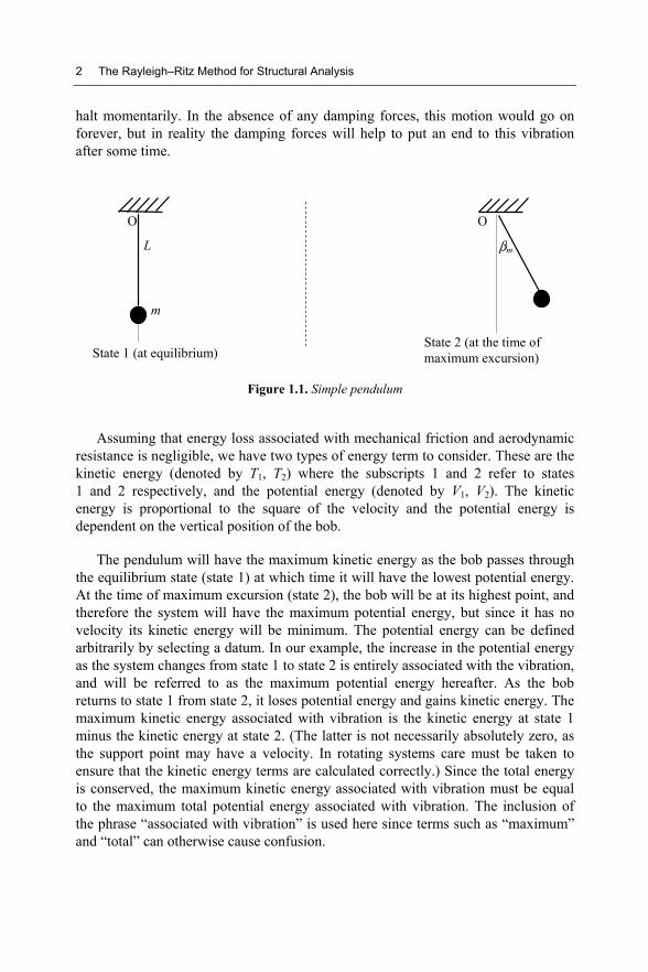
Consider the oscillatory motion of the simple pendulum consisting of a bob of mass m and a massless string of length L as shown in Figure 1.1. It would be at rest in a vertical configuration under gravity field. If it is given a small disturbance βm and then released, it will tend to vibrate about this equilibrium state. The restoring action of the gravity force will initiate a motion toward the equilibrium state but as the bob approaches the lowest point in its motion it has a velocity and therefore carries on swinging up on the other side until the gravity force causes it to come to a

2 The Rayleigh–Ritz Method for Structural Analysis

halt momentarily. In the absence of any damping forces, this motion would go on forever, but in reality the damping forces will help to put an end to this vibration after some time.

Figure 1.1. Simple pendulum

Assuming that energy loss associated with mechanical friction and aerodynamic resistance is negligible, we have two types of energy term to consider. These are the kinetic energy (denoted by T1, T2) where the subscripts 1 and 2 refer to states 1 and 2 respectively, and the potential energy (denoted by V1, V2). The kinetic energy is proportional to the square of the velocity and the potential energy is dependent on the vertical position of the bob.

The pendulum will have the maximum kinetic energy as the bob passes through the equilibrium state (state 1) at which time it will have the lowest potential energy. At the time of maximum excursion (state 2), the bob will be at its highest point, and therefore the system will have the maximum potential energy, but since it has no velocity its kinetic energy will be minimum. The potential energy can be defined arbitrarily by selecting a datum. In our example, the increase in the potential energy as the system changes from state 1 to state 2 is entirely associated with the vibration, and will be referred to as the maximum potential energy hereafter. As the bob returns to state 1 from state 2, it loses potential energy and gains kinetic energy. The maximum kinetic energy associated with vibration is the kinetic energy at state 1 minus the kinetic energy at state 2. (The latter is not necessarily absolutely zero, as the support point may have a velocity. In rotating systems care must be taken to ensure that the kinetic energy terms are calculated correctly.) Since the total energy is conserved, the maximum kinetic energy associated with vibration must be equal to the maximum total potential energy associated with vibration. The inclusion of the phrase “associated with vibration” is used here since terms such as “maximum” and “total” can otherwise cause confusion.

State 1 (at equilibrium)

O

L

m

βm

O

State 2 (at the time of maximum excursion)

Principle of Conservation of Energy and Rayleigh’s Principle 3

From the principle of conservation of energy:

1 1 2 2V T V T+ = +

i.e. 2 1 1 2V V T T− = −

The gain in potential energy as the bob moves from state 1 to state 2 is the maximum potential energy associated with vibration and may be denoted by Vm.

2 1 mV V V− =

Similarly the maximum kinetic energy associated with vibration is:

1 2 mT T T− = [1.1]

From the above equations we have m mV T=

In applying the principle of conservation of energy for vibratory systems, it is sufficient to equate the maximum potential and kinetic energy terms associated with vibration.

To find the circular natural frequency ω of an undamped system, the motion may be assumed to be simple harmonic.

i.e. β = βm sin(ωt+α), where t is time and α is a phase shift angle.

Then ddtβ β= = ωβm cos(ωt+α)

The maximum velocity is therefore = Lωβm

This means the maximum velocity is equal to the amplitude of vibration times the frequency. This statement is true for any natural mode, since at natural modes the vibration is simple harmonic.

Hence 2( )

2m

mL

T mωβ

=

The potential energy is due to the change in position of the gravity force mg.

Thus (1 cos )m mV mgL β= −

4 The Rayleigh–Ritz Method for Structural Analysis

Substituting these into equation [1.1] gives:

2( )(1 cos )

2m

mL

m mgLωβ β= −

For small amplitude vibration, 2

(1 cos )2m

mββ− =

This gives: 2 2( )

2 2m mL

m mgLωβ β

=

This actually gives us two possible solutions. One is that βm = 0. This implies there will not be any motion and is therefore a trivial solution. The other solution is:

ω2 = g/L

in which case 0mβ ≠ and vibration is possible. That is to say, in the absence of any

external force, the system can vibrate freely at a frequency of /g Lω = rad/s. This is therefore the circular natural frequency of the pendulum. The natural frequency in Hz (cycles/s) is 2 / 2f g Lω π π= = . From this point onwards, for simplicity, we will refer to circular natural frequencies as natural frequencies.

The simple pendulum is a “single degree of freedom” system. This means it can only vibrate in one specific mode, in this case, the string and the bob rotating about the equilibrium state. In cases where the mode is defined, the above method yields the exact value of the natural frequency. We will soon see why it is not always possible or convenient to get the exact frequency.

1.2. A spring-mass system

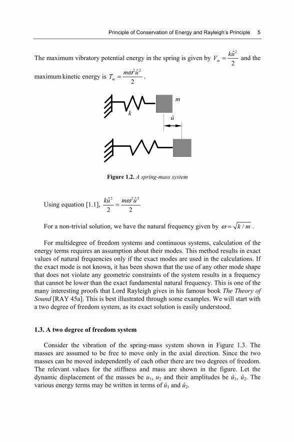
Consider the motion of a simple spring-mass system shown in Figure 1.2. A rigid body of mass m is connected to a linear elastic spring of stiffness k. Assume that the system is free to vibrate only axially (in the direction of the spring). If the mass is displaced from the equilibrium state by distance û which induces a force in the spring and then released, it would tend to return to its equilibrium state. However as it approaches the equilibrium state it has a velocity and this velocity causes the mass to move away from the equilibrium state now on to the opposite side. Then as the spring force develops, the motion comes to an end momentarily and the mass then returns to the equilibrium state and the cycle repeats as in the case of the pendulum.

Principle of Conservation of Energy and Rayleigh’s Principle 5

The maximum vibratory potential energy in the spring is given by 2ˆ

2mkuV = and the

maximum kinetic energy is 2 2ˆ

2mm uT ω= .

Figure 1.2. A spring-mass system

Using equation [1.1], 2 2 2ˆ ˆ

2 2ku m uω=

For a non-trivial solution, we have the natural frequency given by /k mω = .

For multidegree of freedom systems and continuous systems, calculation of the energy terms requires an assumption about their modes. This method results in exact values of natural frequencies only if the exact modes are used in the calculations. If the exact mode is not known, it has been shown that the use of any other mode shape that does not violate any geometric constraints of the system results in a frequency that cannot be lower than the exact fundamental natural frequency. This is one of the many interesting proofs that Lord Rayleigh gives in his famous book The Theory of Sound [RAY 45a]. This is best illustrated through some examples. We will start with a two degree of freedom system, as its exact solution is easily understood.

1.3. A two degree of freedom system

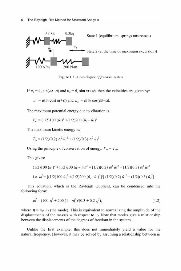
Consider the vibration of the spring-mass system shown in Figure 1.3. The masses are assumed to be free to move only in the axial direction. Since the two masses can be moved independently of each other there are two degrees of freedom. The relevant values for the stiffness and mass are shown in the figure. Let the dynamic displacement of the masses be u1, u2 and their amplitudes be û1, û2. The various energy terms may be written in terms of û1 and û2.

û

m

k

6 The Rayleigh–Ritz Method for Structural Analysis

Figure 1.3. A two degree of freedom system

If u1 = û1 sin(ωt+α) and u2 = û2 sin(ωt+α), then the velocities are given by:

1u = ω û1 cos(ωt+α) and 2u = ω û2 cos(ωt+α).

The maximum potential energy due to vibration is

Vm = (1/2)100 (û1)2 +(1/2)200 (û2 – û1)2

The maximum kinetic energy is:

Tm = (1/2)(0.2) ω2 û12 + (1/2)(0.3) ω2 û2

2

Using the principle of conservation of energy, Vm = Tm.

This gives:

(1/2)100 (û1)2 +(1/2)200 (û2 - û1)2 = (1/2)(0.2) ω2 û12 + (1/2)(0.3) ω2 û2

2

i.e. ω2 = [(1/2)100 û12 +(1/2)200 (û2 - û1)2]/[ (1/2)(0.2) û1

2 + (1/2)(0.3) û22]

This equation, which is the Rayleigh Quotient, can be condensed into the following form:

ω2 = (100 η2 + 200 (1– η)2)/(0.3 + 0.2 η2), [1.2]

where η = û1/ û2 (the mode). This is equivalent to normalizing the amplitude of the displacements of the masses with respect to û2. Note that modes give a relationship between the displacements of the degrees of freedom in the system.

Unlike the first example, this does not immediately yield a value for the natural frequency. However, it may be solved by assuming a relationship between û1

State 1 (equilibrium, springs unstressed)

State 2 (at the time of maximum excursion))

û1 û2

100 N/m 200 N/m

0.2 kg 0.3kg