Embed Size (px)
Citation preview
The Ratchet-Shakedown Diagram for a Thin Pressurised Pipe Subject to
Additional Axial Load and Cyclic Secondary Global Bending
R.A.W.Bradford1 and D.J.Tipping
2
1University of Bristol, Mechanical Engineering, Queen's Building, University Walk, Bristol BS8 1TR, UK, [email protected], tel.+44 1453 843462; 2EDF Energy, Barnett Way, Barnwood, Gloucester, GL4 3RS, [email protected]
Abstract The ratchet and shakedown boundaries are derived analytically for a thin cylinder
composed of elastic-perfectly plastic Tresca material subject to constant internal
pressure with capped ends, plus an additional constant axial load, F, and a cycling
secondary global bending load. The analytic solution in good agreement with solutions
found using the linear matching method. When F is tensile, ratcheting can occur for
sufficiently large cyclic bending loads in which the pipe gets longer and thinner but its
diameter remains the same. When F is compressive, ratcheting can occur in which the
pipe diameter increases and the pipe gets shorter, but its wall thickness remains the
same. When subject to internal pressure and cyclic bending alone (F = 0), no ratcheting
is possible, even for arbitrarily large bending loads, despite the presence of the axial
pressure load. The reason is that the case with a primary axial membrane stress exactly
equal to half the primary hoop membrane stress is equipoised between tensile and
compressive axial ratcheting, and hence does not ratchet at all. This remarkable result
appears to have escaped previous attention.
1. Introduction
A structure subject to two or more types of loading, at least one of which is primary
and at least one of which is cycling, may potentially accumulate deformation which
increases cycle on cycle. This is ratcheting. Rather less severe loading may result in
parts of the structure undergoing plastic cycling, involving a hysteresis loop in stress-
strain space, but without accumulating ratchet strains. Still less severe loading may
result in purely elastic cycling, perhaps after some initial plasticity on the first few
cycles. This is shakedown. It is desirable that engineering structures be in the
shakedown regime since ratcheting is a severe condition leading potentially to failure.
The intermediate case of stable plastic cycling may be structurally acceptable but will
involve the engineer in non-trivial assessments to demonstrate acceptablity, probably
involving the possibility of cracks being initiated by the repeated plastic straining (by
fatigue, and possibly by creep).
Deciding which of the three types of behaviour results from a given loading sequence
on a given structure is, therefore, of considerable importance. Unfortunately
ratcheting/shakedown problems are difficult to solve analytically in the general case.
However, analytical solutions for sufficiently simple geometries and loadings do
exist. One of the earliest, and undoubtedly the most influential, of these is the Bree
problem, Ref.[1]. Bree's analytic solution addresses uniaxial loading of a rectangular
cross section in an elastic-perfectly plastic material, the loading consisting of a
constant primary membrane stress and a secondary bending load which cycles
between zero and some maximum. When normalised by the yield stress, the primary
membrane stress is denoted X whilst the normalised secondary elastic outer fibre
bending stress range is denoted Y .
The ratchet boundary is defined as the curve on an YX , plot above which ratcheting
occurs. Similarly, the shakedown boundary is defined as the curve on the YX , plot
below which shakedown to elastic cycling occurs. The two curves may or may not be
separated by a region of stable plastic cycling. In obvious notation, the three types of
region are denoted R, S and P. Variants on the Bree problem which have been solved
analytically include, (i) the case when the primary membrane load also cycles, either
strictly in-phase or strictly in anti-phase with the secondary bending load, Refs.[2-4],
(ii) the Bree problem with different yield stresses at the two ends of the load cycle,
Ref.[5], and, (iii) the Bree problem with biaxial stressing of a flat plate, an extra
primary membrane load being introduced perpendicular to the Bree loadings, Ref.[6].
The analyses in Refs.[2-6] used the same approach as Bree's original analysis, Ref.[1].
However, alternative, "non-cycling", methods for analytical ratchet boundary
determination are also emerging, e.g., Refs.[7,8].
The difficulty of obtaining analytic solutions for more complicated geometries or
loadings has prompted the development of numerical techniques to address ratcheting
and shakedown. For example, direct cyclic analysis methods, e.g., Ref.[9], can
calculate the stabilised steady-state response of structures with far less computational
effort than full step-by-step analysis. A technique which is now being used widely is
the Linear Matching Method (LMM), e.g., Ref.[10]. LMM is distinguished from other
simplified methods in ensuring that both equilibrium and compatibility are satisfied at
each stage.
This paper presents a Bree-type analysis of the ratchet and shakedown boundaries for
the case of a thin cylinder composed of elastic-perfectly plastic material with internal
pressure and capped ends, plus an additional axial load (F ), together with a global
bending load. The pressure and additional axial loads are constant primary loads. The
global bending is secondary in nature and cycles. The global bending load is
envisaged as arising from a uniform diametral temperature gradient with bending of
the pipe being restrained. The temperature gradient cycles between zero and some
maximum value. After developing the analytic solution for the ratchet and shakedown
boundaries, the solution is verified by use of the LMM technique. (Alternatively this
may be seen as a validation of the LMM technique).
Section 2 formulates the equations which specify the problem. Section 3 defines
normalised, dimensionless quantities which will be used throughout the rest of the
paper. Section 4 describes the method of solution. Sections 5 and 6 present the
solution for the case of tensile ratcheting in the axial direction. Section 7 completes
the solution, considering shakedown and stable plastic cycling as well as compressive
ratcheting in the axial direction. Section 8 describes the numerical analyses carried
out using the LMM method, and finally the key results are summarised in the
Conclusions, Section 9.
Remarkably it will be shown that ratcheting cannot occur if the additional axial load is
zero, 0=F , despite the primary pressure load acting in the axial direction as well as
the hoop direction. This behaviour is probably specific to a straight pipe since
ratcheting of pipe bends due to constant pressure and cyclic global bending has been
analysed in Refs.[11,12].
2. Formulation of the Problem
The notation for stresses and strains in this section will include a tilde, e.g., σ~ , to
distinguish them from the normalised, dimensionless quantities which will be used
hereafter.
The problem considers a thin cylinder so that through-wall stress variations may be
neglected. The cylinder is under internal pressure, P , and an axial load, F . Note that
capped ends ensure that the pressure load also contributes to the total axial load. Both
these primary loads are constant (i.e., not cycling). The cylinder wall is therefore
subject to a constant hoop stress, which is uniform around the circumference, of,
t
H
Pr~=σ (1)
where tr, are the cylinder radius and thickness respectively. The integral of the axial
stress around the cylinder circumference equilibrates the applied axial load plus the
axial pressure load,
∫ ⋅=+= θσπ rtdPrFFTOT
~2 (2)
where σ~ is the axial stress at the angular position θ around the circumference, and
the integral is carried out over the whole circumference. Equ.(2) holds at all times
since the pressure and the additional axial load are constant.
The axial stress is not uniform around the circumference as a consequence of the
cycling secondary bending load. This bending load is envisaged as arising due to a
uniform diametral temperature gradient, i.e., a temperature which varies linearly with
the Cartesian coordinate x~ perpendicular to the cylinder axis. Bending of the cylinder
is taken to be restrained so that the temperature gradient generates a secondary
bending stress. The origin of x~ is taken to be the cylinder axis. The elastically
calculated bending stress is denoted bσ~ , and its tensile side is taken to be 0
~>x .
Hence the elastic bending stress distribution across the pipe diameter would be
rxb
/~~σ where rxr ≤≤−
~ . This secondary bending load cycles between zero and its
maximum value and back again repeatedly.
The material is taken to be elastic-perfectly plastic with yield strength yσ . This is a
common simplifying assumption in such ratcheting analyses, without which the
problem would not be analytically tractable. The Tresca yield criterion is assumed,
again for analytic simplicity. Throughout it will be assumed that the compressive
radial stress on the inner surface is negligible compared with the other stresses, i.e.,
the thin shell limit. Stressing is therefore biaxial.
The hoop stress is necessarily less than yield, yH σσ <~ otherwise the cylinder
collapses. It is worth spelling out why this remains true for this situation of biaxial
stressing. Possible cases are,
• If the axial stress, σ~ , is positive but less than Hσ~ then the Tresca yield criterion
is just yH σσ =~ ;
• If the axial stress, σ~ , is positive and greater than Hσ~ then the Tresca yield
criterion is just yσσ =
~ and hence yielding occurs with yH σσ <~ ;
• If the axial stress, σ~ , is negative then the Tresca yield criterion is yH σσσ =−~~
and hence yielding again occurs with yH σσ <~ .
In all cases, therefore, avoidance of collapse requires yH σσ <~ as a necessary but not
sufficient condition. Consequently, if yH σσ <~ is assumed, in regions where the axial
stress, σ~ , is positive, the yield criterion can be taken to be simply yσσ =
~ . In regions
where the axial stress, σ~ , is negative, the yield criterion becomes Hy σσσ~~
+−= .
Defining the positive quantity Hyy σσσ~
−=′ , the yield criteria are,
For 0~>σ :
yσσ =
~ (3a)
For 0~<σ : yσσ ′−=
~ (3b)
The dimensionless parameter α is defined as,
y
H
y
y
σ
σ
σ
σ
α
~
1−=′
= (4)
Thus, α quantifies the influence of the hoop stress on the ratcheting behaviour.
Consistent with common practice for similar ratcheting analyses the results will be
expressed in terms of the following dimensionless load parameters,
y
TOT
rt
FX
σπ2=
y
bYσ
σ~
= (5)
Because bending of the cylinder is restrained by assumption, the axial strain, ε~ , is
uniform around the circumference. Despite no bending deformation being possible,
nevertheless it is possible for the cylinder to be subject to net axial ratcheting, i.e., if
ε~ increases cycle on cycle. This total axial strain is composed of four parts: the
elastic strain due to the axial stress, the elastic Poisson strain due to the hoop stress,
the plastic strain, and the thermal strain. Hence, if the thermal load is acting,
Thernal Load On: r
x
EEE
bp
H~~
~
~~
~⋅−+−=
σ
ε
σνσ
ε (6a)
where E and ν are the elastic moduli and pε~ is the axial component of plastic strain.
Note that the thermal strain is negative where the thermal stress is tensile, i.e., for
0~>x . There will also be either radial or hoop components of plastic strain, but these
play no part initially in the analysis. The significance of the radial and hoop plastic
strains to the ratcheting behaviour is discussed in §7.
When the thermal load is removed, (6a) becomes,
Thermal Load Off: p
H
EEε
σνσ
ε~
~~
~+−= (6b)
Equations (6a,b) together with the equilibrium condition, (2), and the yield criteria,
(3a,b), suffice to solve the problem.
3. Dimensionless Form
It is convenient to work with dimensionless quantities, normalising all stresses by yσ
and all strains by Eyy /σε = , and the position coordinate by the radius, r . For
example, yσσσ /
~= , yHH σσσ /
~= , yE σεε /
~= ,
yppE σεε /~
= , rxx /~= . Using
also the normalised loads, (5), the equilibrium equation, (2), and the expressions
(6a,b) for the axial strain become,
Thermal Load On: xYpH −+−= ενσσε (7a)
Thermal Load Off: pH ενσσε +−= (7b)
Equilibrium: ∫ ⋅= θσπ
dX2
1 (8)
Whilst the yield criteria are,
For 0>σ : 1=σ (9a)
For 0<σ : ασ −= (9b)
From here on all quantities are understood to be in this normalised form.
4. Solution Method
The method follows the now traditional approach of Refs.[1-6]. It is simplest to
implement by translating the algebraic relations, (7-9), into a geometric description of
the piece-wise linear stress and plastic strain distributions. The key to this is the
requirement that ε be independent of x . The rules that permit construction of the
distributions are,
1) If the thermal load is acting, then, at all points x ,
� Either, the slope of the σ versus x graph is zero and the slope of the p
ε
versus x graph is Y ,
� Or, the slope of the σ versus x graph is Y and the slope of the p
ε versus
x graph is zero.
2) If the thermal load is not acting, then, at all points x ,
� Either, the slope of the σ versus x graph is zero and the slope of the p
ε
versus x graph is also zero,
� Or, the slope of the σ versus x graph is Y− and the slope of the p
ε
versus x graph is Y ,
3) If the stress is in the elastic range, 1<<− σα , then the plastic strain, p
ε , is
unchanged from its value on the last half-cycle.
5. Solution for Figure 1
Figure 1 illustrates the stress distributions in the case that yielding occurs on both
diametrically opposite points 1=x and 1−=x . Because the primary loads are
constant, the stress distributions with and without the thermal load present are mirror
images. The qualitative form of the plastic strain distributions follows from the rules
of §4 and have been illustrated for the first three half-cycles (noting that half cycle 1
has the thermal load acting, half cycle 2 has no thermal load, half cycle 3 has the
thermal load reinstated, etc). The rules of §4 are sufficient to demonstrate that the
assumed stress distributions lead to ratcheting, the ratchet strain being illustrated in
Figure 1. Algebraically the ratchet strain is,
Ybrat
2−=ε (10)
For ratcheting to occur it is therefore required that 0<b , which, referring to Figure 1,
simply means that all parts of the cross-section yield in tension under one or other of
the loading conditions. The ratchet boundary corresponding to Figure 1 is thus
specified by,
0=b (11)
To solve for the unknown dimensions a and b note that the slope of the elastic part
of the stress distribution on the first half-cycle must be Y so that the stress in this
region is given explicitly by,
For bxa << : ( )bxY −+=1σ (12)
At ax = this implies, ( )baY −+=− 1α (13)
The angular positions corresponding to ax = and bx = are aθ and
bθ respectively,
where, for dimensions normalised by r , we have simply aa
1sin
−
=θ and bb
1sin
−
=θ .
The equilibrium equation (8) becomes,
( ) ( )[ ]
+−++−= ∫∫∫−
2/
2/
.1sin11
π
θ
θ
θ
θ
π
θθθθαπ
b
b
a
a
ddbYdX (14)
Carrying out the integrals gives,
( ) ( )ba
abab YYbX θθ
ππ
θ
π
θ
π
θα
π
θcoscos1
2
1
2
1−+
−−+
+−−= (15)
In general the dimensions a and b could be found by numerical solution of the
simultaneous equations (13) and (15) for any given loads X and Y consistent with the
ratcheting condition of Figure 1. Equ.(10) would then provide the ratchet strain per
cycle. Our present purpose is only to determine the ratchet boundary, given by (11).
On the ratchet boundary ( 0=b ) (13) and (15) become,
R2 ratchet boundary:
+−=
Ya
α1 and ( ) ( ) ( )1cos11
2
1−++−−=
a
aY
X θπ
απ
θα (16)
Substituting the first of equs.(16) into the second provides an equation for X in terms
of Y which is the ratchet boundary on the ( )YX , diagram. The resulting ratchet
boundaries are plotted as the pink curves in Figures 3-6 for α values of 0.7, 0.5, 0.3
and 0.1 respectively. (These correspond to hoop stresses of 30%, 50%, 70% and 90%
of yield respectively).
For Figure 1 to apply, a must lie in the range -1 to 0. The condition 1−>a implies,
due to (16),
On R2 ratchet boundary, ⇒−> 1a π
α+
−<
11X and α+>1Y (17)
Hence the ratchet boundaries corresponding to Figure 1 and Equs.(16) apply only in
the parameter range indicated by (17), i.e., the pink part of the curves in Figures 3-6.
Following Bree, the region above this ratchet boundary is denoted R2.
The left-hand extreme of the pink curves is given by 0→a and (16) then gives,
On R2 ratchet boundary, ⇒→ 0a ( )α−→ 12
1X and ∞→Y (18)
Hence the ratchet boundary has a vertical asymptote at ( )α−= 12
1X . This is the case
that there is no additional axial load, 0=F , when the axial load is that due to
pressure only, thus,
( ) P
a
HX σ
σ
α =⋅=−→2
12
1 (19)
where P
aσ is the axial membrane stress due to pressure (normalised by yield). Figures
3-6 show this vertical asymptote as the dashed pink line. This leads to the remarkable
conclusion that ratcheting is not possible if no axial load other than that due to
pressure is applied. The physical reason for this is discussed in §7.
Figures 3-6 also show the ratchet boundary for the case 1=α (i.e., zero pressure) for
comparison (green dashed curves). Note that this case is similar to the original Bree
problem, Ref.[1], except for the cylindrical geometry. For small X the ratchet
boundary for the case 1=α tends to π/2=XY and hence gives ∞→Y only as 0→X .
We expect to find another ratcheting region, corresponding to R1 on the Bree
diagram, for which Figure 2 illustrates the candidate stress and plastic strain
distributions. The boundary between the two occurs when 1−=a on Figure 1 (or
equivalently, ασ −=1
on Figure 2). From (13) and (15) this gives,
bY
+
+=
1
1 α and ( )
b
bbY
YX θππ
θα
π
θcos
2
1
2
1−
+−+−= (20)
The R1/R2 boundary curve is determined parametrically over b by (20). This
boundary between the R1 and R2 regions is shown on Figures 3-6 as the continuous
blue curve. (The corresponding R1/R2 boundary for the case 1=α is the dashed blue
curve).
6. Solution for Figure 2
It is clear from Figure 2 that the ratchet strain is again given by (10) though b will be
different. The slope of the elastic part of the stress distribution for the first half-cycle
in Figure 2 gives,
b
Y+
−
=
1
11σ
(21)
This provides one relationship between the unknown quantities b and 1σ . A second
relationship is provided by the equilibrium equation, (8), which in this case gives,
( )[ ]
+−+= ∫∫−
2/
2/
.1sin11
π
θ
θ
π
θθθπ
b
b
ddbYX (22a)
Hence, ( )b
bbY
YbX θππ
θ
π
θcos
2
11
2
1−
+−+−= (22b)
Eqn.(22b) determines b in terms of X and Y , and the ratchet strain is then given by
(10) and 1σ by (21). Figures 1 and 2 become the same when ασ −=
1 and this
condition when substituted into (21) and (22b) reproduces the R1/R2 boundary given
by (20) - as it should for consistency.
It is clear from Figure 2 that ratcheting occurs if and only if 0<b . Hence the ratchet
boundary in the R1 region is given by substituting 0=b into (21) and (22b) giving,
R1 Ratchet Boundary: 1=+π
YX (23)
This compares to the original Bree ratchet boundary in region R1 which is 14=+
YX .
Unlike in region R2, in region R1 the ratchet boundary is independent of α , i.e., it is
independent of the hoop stress.
Figure 2 is applicable only if ασ −>1
and substituting this condition into 1
1 σ−=Y
and (23) gives the complement of (17), i.e.,
On R1 ratchet boundary: π
α+−>1
1X and α+< 1Y (24)
which again confirms consistency with the R2 region ratchet boundary.
The ratchet boundaries for α values of 0.1, 0.2, 0.3.... to 1 are compared on Figure 7.
Note that Figures 3-7 show only the regions where ratcheting produces tensile plastic
straining in the axial direction, for ( ) 2/1 α−>X . For values of X less than
( ) 2/1 α− the additional axial load is compressive, 0<F . Ratcheting in this region is
discussed in §7.
7. The Complete 'Universal' Ratchet-Shakedown Diagram
So far we have derived only the ratcheting solution but not the shakedown solution,
nor what regions of the YX , diagram give rise to stable plastic cycling. Moreover,
the ratcheting solution has been found only for the case of tensile ratcheting in the
axial direction. We may complete the solution very quickly by appeal to the similarity
of the present problem with that of Ref.[6], the two problems differing only in the
cylindrical geometry of the present problem in contrast to the flat plate considered in
Ref.[6]. It may be observed that our eqns.(7-9) are essentially the same as the
corresponding equations of Ref.[6], except that the linear integrations over dz in the
latter are replaced by circular (trignometric) integrals over θd in the present case.
A rather elegant solution to the complete problem in Ref.[6] was found by allowing
X to take negative values. This corresponds in the present problem to considering
additional axial loads which are compressive and exceed the axial pressure load, so
that the net axial stress is also compressive. Ref.[6] identified nine qualitatively
different stress and plastic strain distributions corresponding to nine different regions
of the ratchet-shakedown diagram. This showed that for ( ) 2/1 α−<X there are
ratcheting regions where the axial ratchet strain is compressive. Moreover the overall
ratchet-shakedown diagram has a mirror plane of symmetry at ( ) 2/1 α−=X . Since
we already have the solution for ( ) 2/1 α−>X this allows us to deduce immediately
the complete solution.
In addition, Ref.[6] showed that the ratchet-shakedown diagrams for different α
become a single, 'universal', diagram applicable for all α if the YX , axes are
suitably redefined. The redefinition used in Ref.[6] to accomplish this was,
α
α
+
+=′
1
XX and
α+=′
1
YY (25)
This same redefinition also removes the α dependence from the ratchet boundary
curves for the present problem, as may readily be proved by substitution of (25) into
(23) and (16) which respectively become,
R1 ratchet boundary: 1=′
+′π
YX (26)
R2 ratchet boundary:
′+′−−′+=′ −
YYYX
1sin1
1
2
1 12
π
(27)
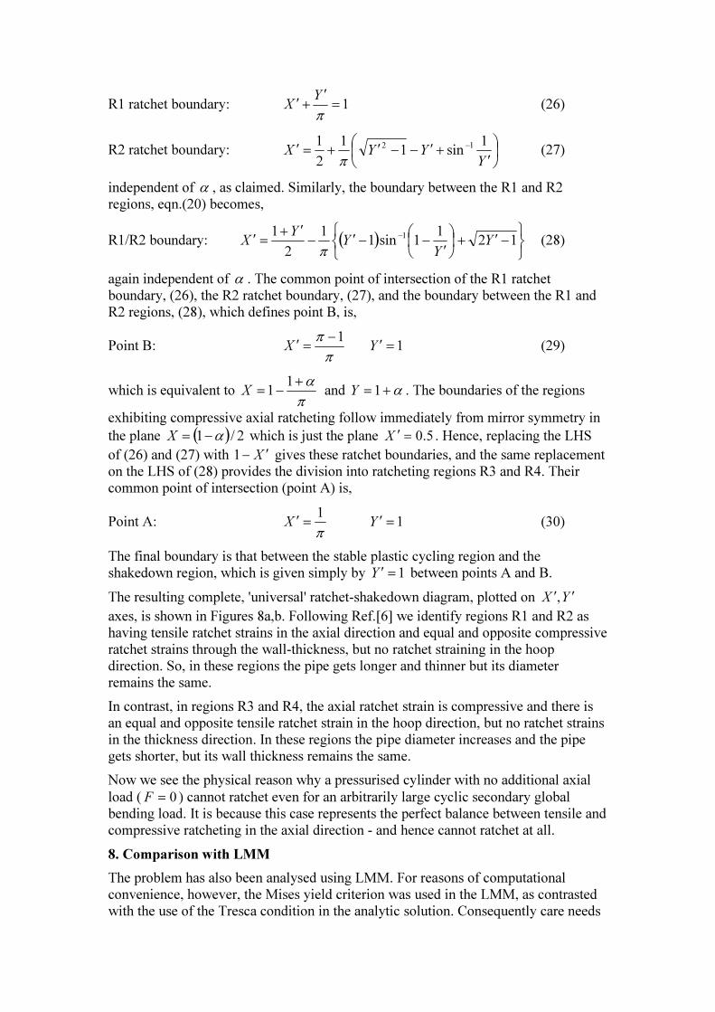
independent of α , as claimed. Similarly, the boundary between the R1 and R2
regions, eqn.(20) becomes,
R1/R2 boundary: ( )
−′+
′−−′−
′+=′ −
121
1sin11
2
1 1Y
YY
YX
π
(28)
again independent of α . The common point of intersection of the R1 ratchet
boundary, (26), the R2 ratchet boundary, (27), and the boundary between the R1 and
R2 regions, (28), which defines point B, is,
Point B: π
π 1−=′X 1=′Y (29)
which is equivalent to π
α+−=1
1X and α+= 1Y . The boundaries of the regions
exhibiting compressive axial ratcheting follow immediately from mirror symmetry in
the plane ( ) 2/1 α−=X which is just the plane 5.0=′X . Hence, replacing the LHS
of (26) and (27) with X ′−1 gives these ratchet boundaries, and the same replacement
on the LHS of (28) provides the division into ratcheting regions R3 and R4. Their
common point of intersection (point A) is,
Point A: π
1=′X 1=′Y (30)
The final boundary is that between the stable plastic cycling region and the
shakedown region, which is given simply by 1=′Y between points A and B.
The resulting complete, 'universal' ratchet-shakedown diagram, plotted on YX ′′,
axes, is shown in Figures 8a,b. Following Ref.[6] we identify regions R1 and R2 as
having tensile ratchet strains in the axial direction and equal and opposite compressive
ratchet strains through the wall-thickness, but no ratchet straining in the hoop
direction. So, in these regions the pipe gets longer and thinner but its diameter
remains the same.
In contrast, in regions R3 and R4, the axial ratchet strain is compressive and there is
an equal and opposite tensile ratchet strain in the hoop direction, but no ratchet strains
in the thickness direction. In these regions the pipe diameter increases and the pipe
gets shorter, but its wall thickness remains the same.
Now we see the physical reason why a pressurised cylinder with no additional axial
load ( 0=F ) cannot ratchet even for an arbitrarily large cyclic secondary global
bending load. It is because this case represents the perfect balance between tensile and
compressive ratcheting in the axial direction - and hence cannot ratchet at all.
8. Comparison with LMM
The problem has also been analysed using LMM. For reasons of computational
convenience, however, the Mises yield criterion was used in the LMM, as contrasted
with the use of the Tresca condition in the analytic solution. Consequently care needs
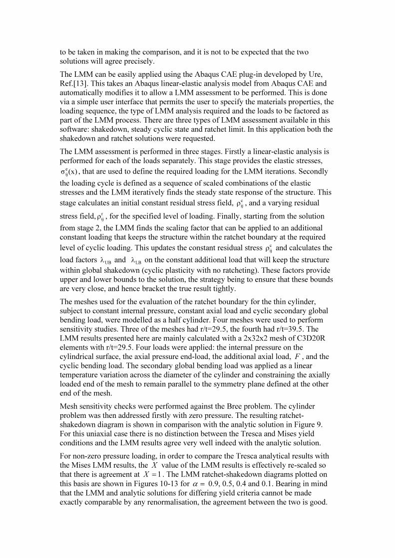
to be taken in making the comparison, and it is not to be expected that the two
solutions will agree precisely.
The LMM can be easily applied using the Abaqus CAE plug-in developed by Ure,
Ref.[13]. This takes an Abaqus linear-elastic analysis model from Abaqus CAE and
automatically modifies it to allow a LMM assessment to be performed. This is done
via a simple user interface that permits the user to specify the materials properties, the
loading sequence, the type of LMM analysis required and the loads to be factored as
part of the LMM process. There are three types of LMM assessment available in this
software: shakedown, steady cyclic state and ratchet limit. In this application both the
shakedown and ratchet solutions were requested.
The LMM assessment is performed in three stages. Firstly a linear-elastic analysis is
performed for each of the loads separately. This stage provides the elastic stresses,
)(xσeij , that are used to define the required loading for the LMM iterations. Secondly
the loading cycle is defined as a sequence of scaled combinations of the elastic
stresses and the LMM iteratively finds the steady state response of the structure. This
stage calculates an initial constant residual stress field, cijρ , and a varying residual
stress field, rijρ , for the specified level of loading. Finally, starting from the solution
from stage 2, the LMM finds the scaling factor that can be applied to an additional
constant loading that keeps the structure within the ratchet boundary at the required
level of cyclic loading. This updates the constant residual stress cijρ and calculates the
load factors UB
λ and LB
λ on the constant additional load that will keep the structure
within global shakedown (cyclic plasticity with no ratcheting). These factors provide
upper and lower bounds to the solution, the strategy being to ensure that these bounds
are very close, and hence bracket the true result tightly.
The meshes used for the evaluation of the ratchet boundary for the thin cylinder,
subject to constant internal pressure, constant axial load and cyclic secondary global
bending load, were modelled as a half cylinder. Four meshes were used to perform
sensitivity studies. Three of the meshes had r/t=29.5, the fourth had r/t=39.5. The
LMM results presented here are mainly calculated with a 2x32x2 mesh of C3D20R
elements with r/t=29.5. Four loads were applied: the internal pressure on the
cylindrical surface, the axial pressure end-load, the additional axial load, F , and the
cyclic bending load. The secondary global bending load was applied as a linear
temperature variation across the diameter of the cylinder and constraining the axially
loaded end of the mesh to remain parallel to the symmetry plane defined at the other
end of the mesh.
Mesh sensitivity checks were performed against the Bree problem. The cylinder
problem was then addressed firstly with zero pressure. The resulting ratchet-
shakedown diagram is shown in comparison with the analytic solution in Figure 9.
For this uniaxial case there is no distinction between the Tresca and Mises yield
conditions and the LMM results agree very well indeed with the analytic solution.
For non-zero pressure loading, in order to compare the Tresca analytical results with
the Mises LMM results, the X value of the LMM results is effectively re-scaled so
that there is agreement at 1=X . The LMM ratchet-shakedown diagrams plotted on
this basis are shown in Figures 10-13 for =α 0.9, 0.5, 0.4 and 0.1. Bearing in mind
that the LMM and analytic solutions for differing yield criteria cannot be made
exactly comparable by any renormalisation, the agreement between the two is good.
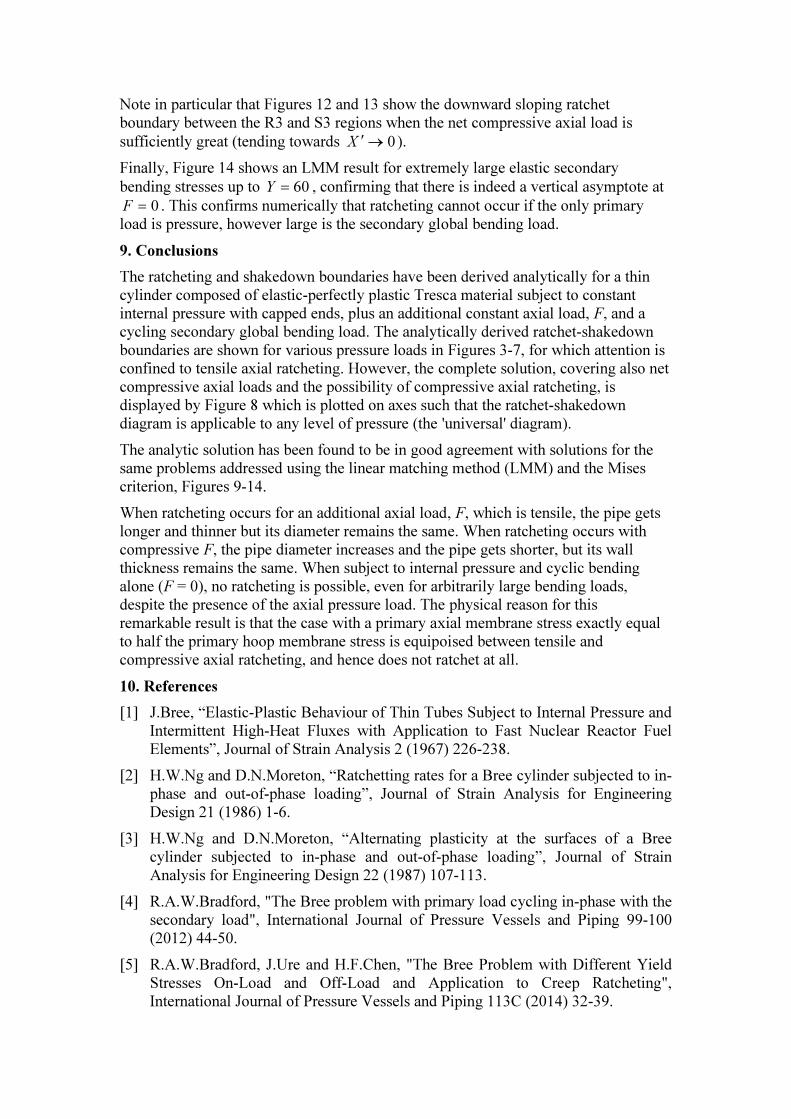
Note in particular that Figures 12 and 13 show the downward sloping ratchet
boundary between the R3 and S3 regions when the net compressive axial load is
sufficiently great (tending towards 0→′X ).
Finally, Figure 14 shows an LMM result for extremely large elastic secondary
bending stresses up to 60=Y , confirming that there is indeed a vertical asymptote at
0=F . This confirms numerically that ratcheting cannot occur if the only primary
load is pressure, however large is the secondary global bending load.
9. Conclusions
The ratcheting and shakedown boundaries have been derived analytically for a thin
cylinder composed of elastic-perfectly plastic Tresca material subject to constant
internal pressure with capped ends, plus an additional constant axial load, F, and a
cycling secondary global bending load. The analytically derived ratchet-shakedown
boundaries are shown for various pressure loads in Figures 3-7, for which attention is
confined to tensile axial ratcheting. However, the complete solution, covering also net
compressive axial loads and the possibility of compressive axial ratcheting, is
displayed by Figure 8 which is plotted on axes such that the ratchet-shakedown
diagram is applicable to any level of pressure (the 'universal' diagram).
The analytic solution has been found to be in good agreement with solutions for the
same problems addressed using the linear matching method (LMM) and the Mises
criterion, Figures 9-14.
When ratcheting occurs for an additional axial load, F, which is tensile, the pipe gets
longer and thinner but its diameter remains the same. When ratcheting occurs with
compressive F, the pipe diameter increases and the pipe gets shorter, but its wall
thickness remains the same. When subject to internal pressure and cyclic bending
alone (F = 0), no ratcheting is possible, even for arbitrarily large bending loads,
despite the presence of the axial pressure load. The physical reason for this
remarkable result is that the case with a primary axial membrane stress exactly equal
to half the primary hoop membrane stress is equipoised between tensile and
compressive axial ratcheting, and hence does not ratchet at all.
10. References
[1] J.Bree, “Elastic-Plastic Behaviour of Thin Tubes Subject to Internal Pressure and Intermittent High-Heat Fluxes with Application to Fast Nuclear Reactor Fuel
Elements”, Journal of Strain Analysis 2 (1967) 226-238.
[2] H.W.Ng and D.N.Moreton, “Ratchetting rates for a Bree cylinder subjected to in-
phase and out-of-phase loading”, Journal of Strain Analysis for Engineering
Design 21 (1986) 1-6.
[3] H.W.Ng and D.N.Moreton, “Alternating plasticity at the surfaces of a Bree
cylinder subjected to in-phase and out-of-phase loading”, Journal of Strain
Analysis for Engineering Design 22 (1987) 107-113.
[4] R.A.W.Bradford, "The Bree problem with primary load cycling in-phase with the
secondary load", International Journal of Pressure Vessels and Piping 99-100
(2012) 44-50.
[5] R.A.W.Bradford, J.Ure and H.F.Chen, "The Bree Problem with Different Yield
Stresses On-Load and Off-Load and Application to Creep Ratcheting",
International Journal of Pressure Vessels and Piping 113C (2014) 32-39.
[6] R.A.W.Bradford, "Solution of the Ratchet-Shakedown Bree Problem with an
Extra Orthogonal Primary Load", International Journal of Pressure Vessels and
Piping (in press, available on-line 11 March 2015).
[7] Reinhardt, W., "A Non-Cyclic Method for Plastic Shakedown Analysis". ASME
J. Press. Vessel Technol. 130(3) (2008) paper 031209.
[8] Adibi-Asl, R., Reinhardt, W., "Non-cyclic shakedown/ratcheting boundary
determination part 1: analytical approach". International Journal of Pressure
Vessels and Piping 88 (2011) 311-320.
[9] Jiang W, Leckie FA. A direct method for the shakedown analysis of structures
under sustained and cyclic loads. Journal of Applied Mechanics 59 (1992) 251-
60.
[10] Chen H, Ponter ARS. Linear matching method on the evaluation of plastic and
creep behaviours for bodies subjected to cyclic thermal and mechanical loading.
International Journal of Numerical Methods in Engineering 68 (2006) 13-32.
[11] Haofeng Chen, James Ure, Tianbai Li, Weihang Chen, Donald Mackenzie,
"Shakedown and limit analysis of 90° pipe bends under internal pressure, cyclic
in-plane bending and cyclic thermal loading", International Journal of Pressure
Vessels and Piping 88 (2011) 213-222.
[12] Hany F. Abdalla, "Shakedown boundary determination of a 90° back-to-back
pipe bend subjected to steady internal pressures and cyclic in-plane bending
moments", International Journal of Pressure Vessels and Piping 116 (2014) 1-9.
[13] J.M.Ure, “An Advanced Lower and Upper Bound Shakedown Analysis Method
to Enhance the R5 High Temperature Assessment Procedure”, University of
Strathclyde, Thesis submitted for Doctor of Engineering (EngD) in Nuclear
Engineering, (2013).
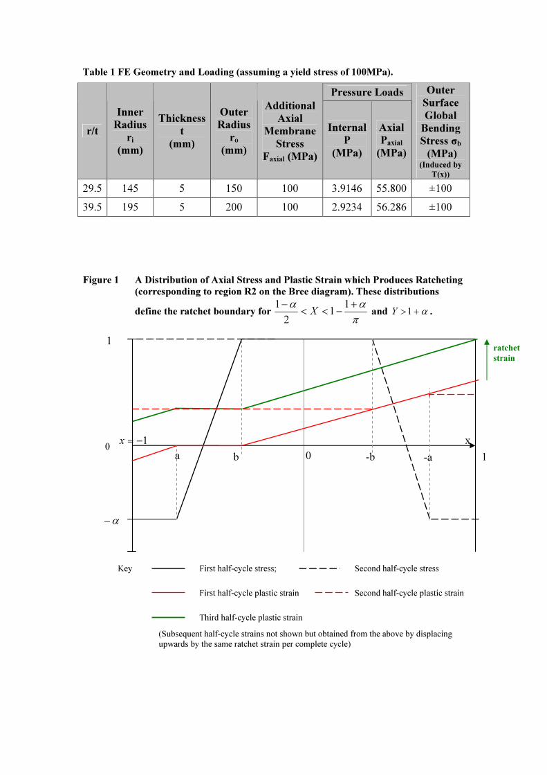
Table 1 FE Geometry and Loading (assuming a yield stress of 100MPa).
Pressure Loads
r/t
Inner
Radius
ri
(mm)
Thickness
t
(mm)
Outer
Radius
ro
(mm)
Additional
Axial
Membrane
Stress
Faxial (MPa)
Internal
P
(MPa)
Axial
Paxial
(MPa)
Outer
Surface
Global
Bending
Stress σb
(MPa) (Induced by
T(x))
29.5 145 5 150 100 3.9146 55.800 ±100
39.5 195 5 200 100 2.9234 56.286 ±100
Figure 1 A Distribution of Axial Stress and Plastic Strain which Produces Ratcheting
(corresponding to region R2 on the Bree diagram). These distributions
define the ratchet boundary for π
αα +−<<
− 11
2
1X and α+>1Y .
1−=x
1
1
α−
b 0
Key First half-cycle stress; Second half-cycle stress
First half-cycle plastic strain Second half-cycle plastic strain
-b -a
ratchet
strain
Third half-cycle plastic strain
(Subsequent half-cycle strains not shown but obtained from the above by displacing
upwards by the same ratchet strain per complete cycle)
a 0
x
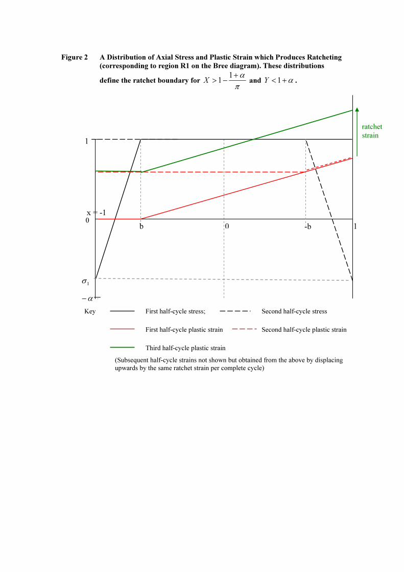
Figure 2 A Distribution of Axial Stress and Plastic Strain which Produces Ratcheting
(corresponding to region R1 on the Bree diagram). These distributions
define the ratchet boundary for π
α+−>1
1X and α+< 1Y .
x = -1
1
1
α−
b 0
Key First half-cycle stress; Second half-cycle stress
First half-cycle plastic strain Second half-cycle plastic strain
-b
Third half-cycle plastic strain
(Subsequent half-cycle strains not shown but obtained from the above by displacing
upwards by the same ratchet strain per complete cycle)
1σ
0
ratchet
strain
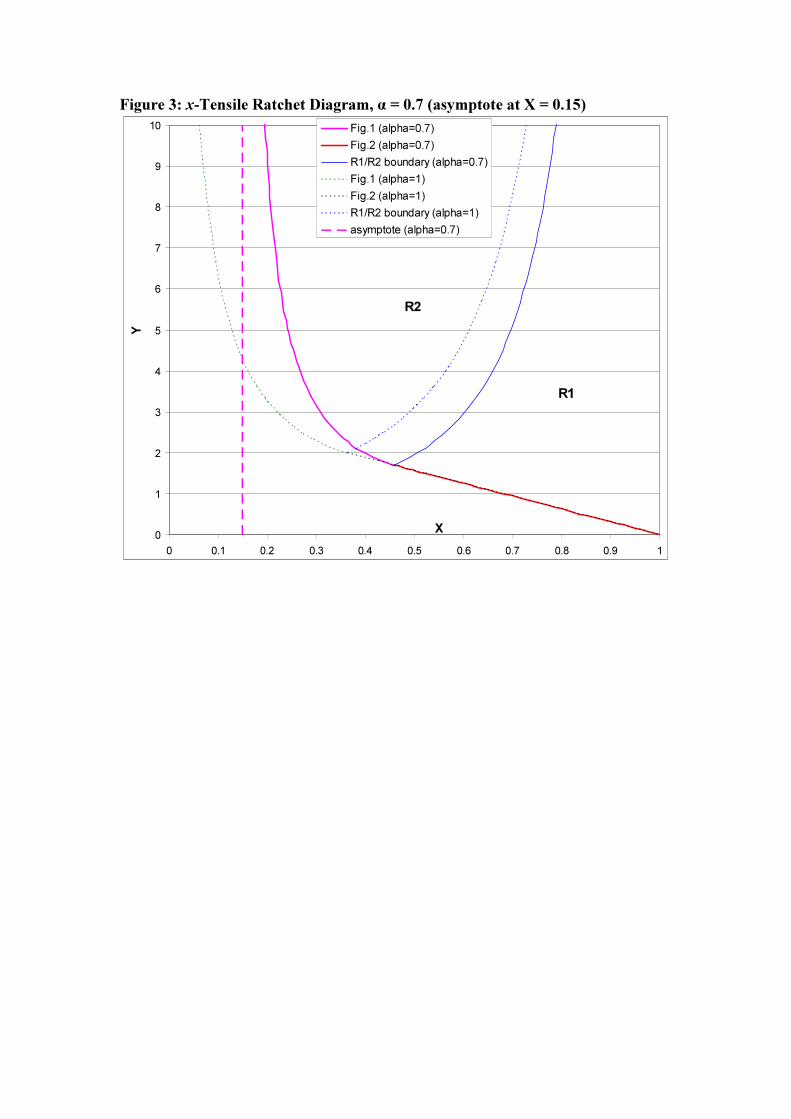
Figure 3: x-Tensile Ratchet Diagram, α = 0.7 (asymptote at X = 0.15)
0
1
2
3
4
5
6
7
8
9
10
0 0.1 0.2 0.3 0.4 0.5 0.6 0.7 0.8 0.9 1
X
YFig.1 (alpha=0.7)
Fig.2 (alpha=0.7)
R1/R2 boundary (alpha=0.7)
Fig.1 (alpha=1)
Fig.2 (alpha=1)
R1/R2 boundary (alpha=1)
asymptote (alpha=0.7)
R2
R1
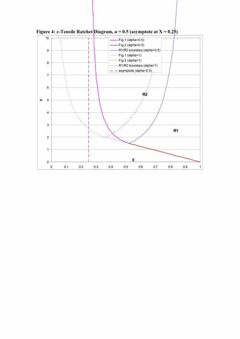
Figure 4: x-Tensile Ratchet Diagram, α = 0.5 (asymptote at X = 0.25)
0
1
2
3
4
5
6
7
8
9
10
0 0.1 0.2 0.3 0.4 0.5 0.6 0.7 0.8 0.9 1
X
YFig.1 (alpha=0.5)
Fig.2 (alpha=0.5)
R1/R2 boundary (alpha=0.5)
Fig.1 (alpha=1)
Fig.2 (alpha=1)
R1/R2 boundary (alpha=1)
asymptote (alpha=0.5)
R2
R1
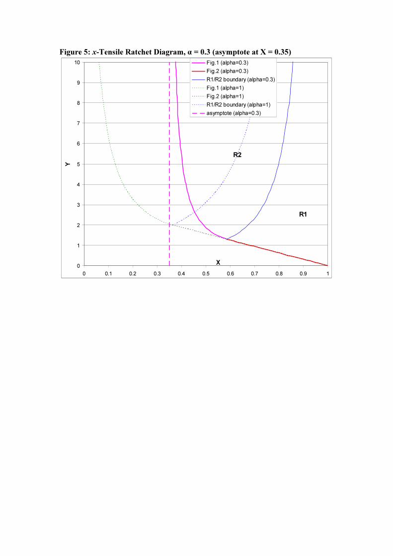
Figure 5: x-Tensile Ratchet Diagram, α = 0.3 (asymptote at X = 0.35)
0
1
2
3
4
5
6
7
8
9
10
0 0.1 0.2 0.3 0.4 0.5 0.6 0.7 0.8 0.9 1
X
YFig.1 (alpha=0.3)
Fig.2 (alpha=0.3)
R1/R2 boundary (alpha=0.3)
Fig.1 (alpha=1)
Fig.2 (alpha=1)
R1/R2 boundary (alpha=1)
asymptote (alpha=0.3)
R2
R1
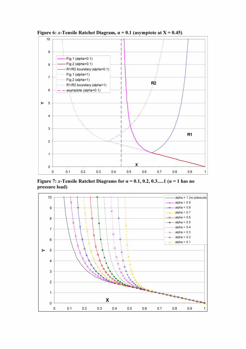
Figure 6: x-Tensile Ratchet Diagram, α = 0.1 (asymptote at X = 0.45)
0
1
2
3
4
5
6
7
8
9
10
0 0.1 0.2 0.3 0.4 0.5 0.6 0.7 0.8 0.9 1
X
Y
Fig.1 (alpha=0.1)
Fig.2 (alpha=0.1)
R1/R2 boundary (alpha=0.1)
Fig.1 (alpha=1)
Fig.2 (alpha=1)
R1/R2 boundary (alpha=1)
asymptote (alpha=0.1)
R2
R1
Figure 7: x-Tensile Ratchet Diagrams for α = 0.1, 0.2, 0.3.....1 (α = 1 has no
pressure load)
0
1
2
3
4
5
6
7
8
9
10
0 0.1 0.2 0.3 0.4 0.5 0.6 0.7 0.8 0.9 1
X
Y
alpha = 1 (no pressure)
alpha = 0.9
alpha = 0.8
alpha = 0.7
alpha = 0.6
alpha = 0.5
alpha = 0.4
alpha = 0.3
alpha = 0.2
alpha = 0.1
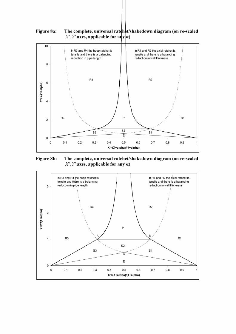
Figure 8a: The complete, universal ratchet/shakedown diagram (on re-scaled
YX ′′, axes, applicable for any α)
0
2
4
6
8
10
0 0.1 0.2 0.3 0.4 0.5 0.6 0.7 0.8 0.9 1
X'=(X+alpha)/(1+alpha)
Y'=Y/(1+alpha)
R2
R1R3
R4
P
E
S2S1S3
In R1 and R2 the axial ratchet is
tensile and there is a balancing
reduction in wall thickness
In R3 and R4 the hoop ratchet is
tensile and there is a balancing
reduction in pipe length
Figure 8b: The complete, universal ratchet/shakedown diagram (on re-scaled
YX ′′, axes, applicable for any α)
0
1
2
3
0 0.1 0.2 0.3 0.4 0.5 0.6 0.7 0.8 0.9 1
X'=(X+alpha)/(1+alpha)
Y'=Y/(1+alpha)
R2
R1R3
R4
P
E
S2
S1S3
A B
C
In R1 and R2 the axial ratchet is
tensile and there is a balancing
reduction in wall thickness
In R3 and R4 the hoop ratchet is
tensile and there is a balancing
reduction in pipe length
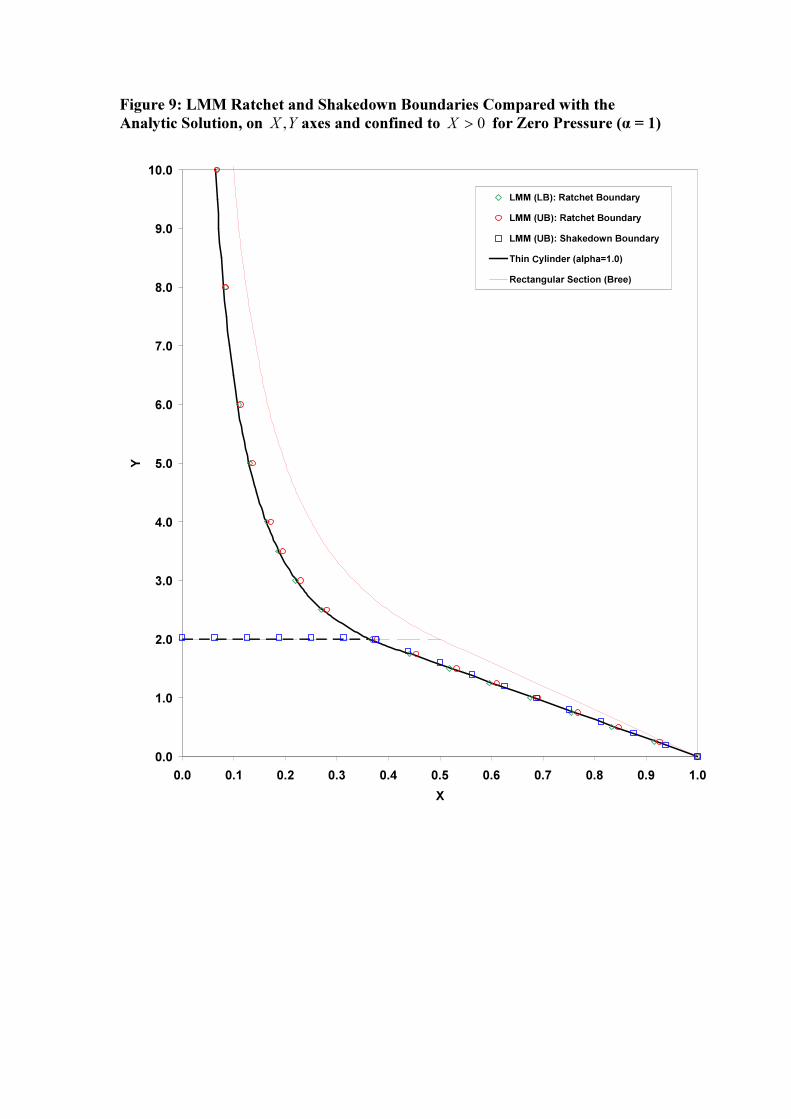
Figure 9: LMM Ratchet and Shakedown Boundaries Compared with the
Analytic Solution, on YX , axes and confined to 0>X for Zero Pressure (α = 1)
0.0
1.0
2.0
3.0
4.0
5.0
6.0
7.0
8.0
9.0
10.0
0.0 0.1 0.2 0.3 0.4 0.5 0.6 0.7 0.8 0.9 1.0
X
Y
LMM (LB): Ratchet Boundary
LMM (UB): Ratchet Boundary
LMM (UB): Shakedown Boundary
Thin Cylinder (alpha=1.0)
Rectangular Section (Bree)
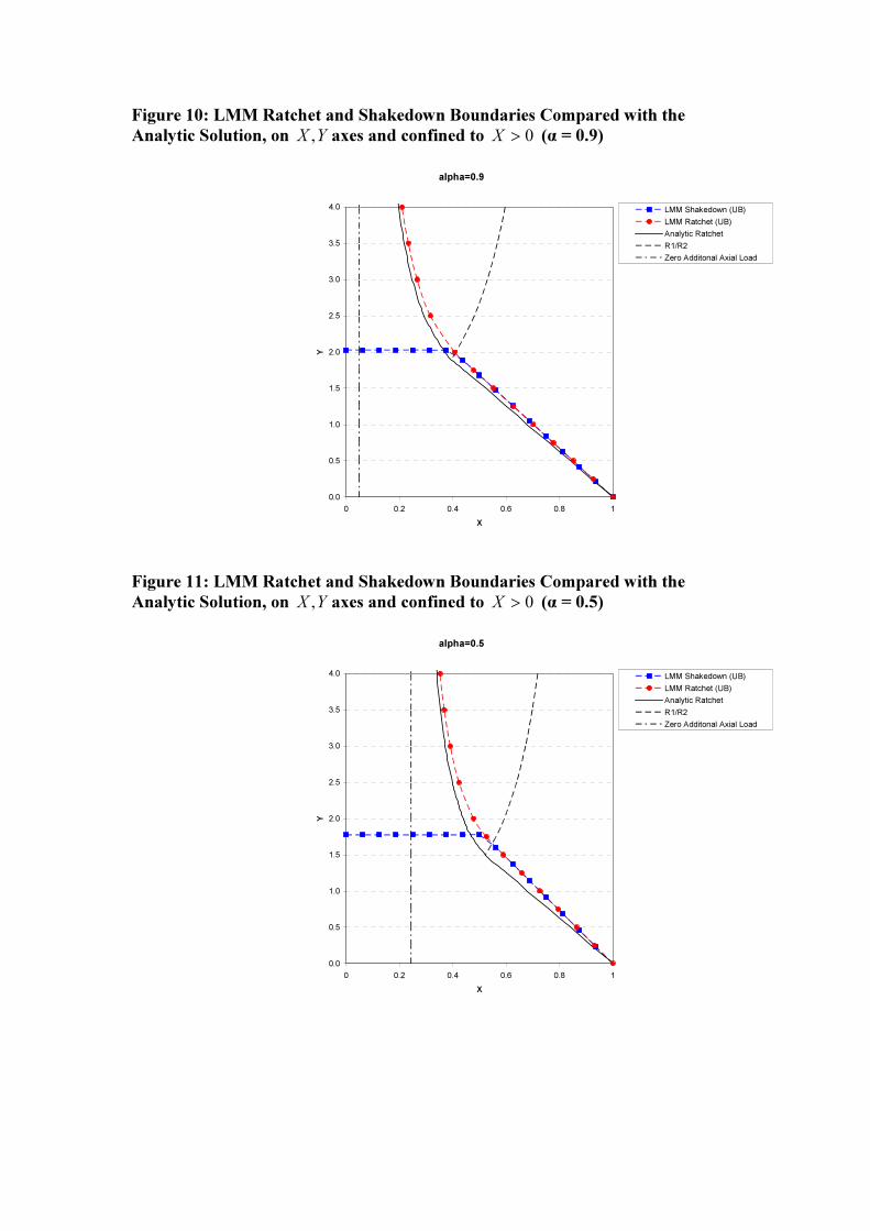
Figure 10: LMM Ratchet and Shakedown Boundaries Compared with the
Analytic Solution, on YX , axes and confined to 0>X (α = 0.9)
alpha=0.9
0.0
0.5
1.0
1.5
2.0
2.5
3.0
3.5
4.0
0 0.2 0.4 0.6 0.8 1
X
Y
LMM Shakedown (UB)
LMM Ratchet (UB)
Analytic Ratchet
R1/R2
Zero Additonal Axial Load
Figure 11: LMM Ratchet and Shakedown Boundaries Compared with the
Analytic Solution, on YX , axes and confined to 0>X (α = 0.5)
alpha=0.5
0.0
0.5
1.0
1.5
2.0
2.5
3.0
3.5
4.0
0 0.2 0.4 0.6 0.8 1
X
Y
LMM Shakedown (UB)
LMM Ratchet (UB)
Analytic Ratchet
R1/R2
Zero Additonal Axial Load
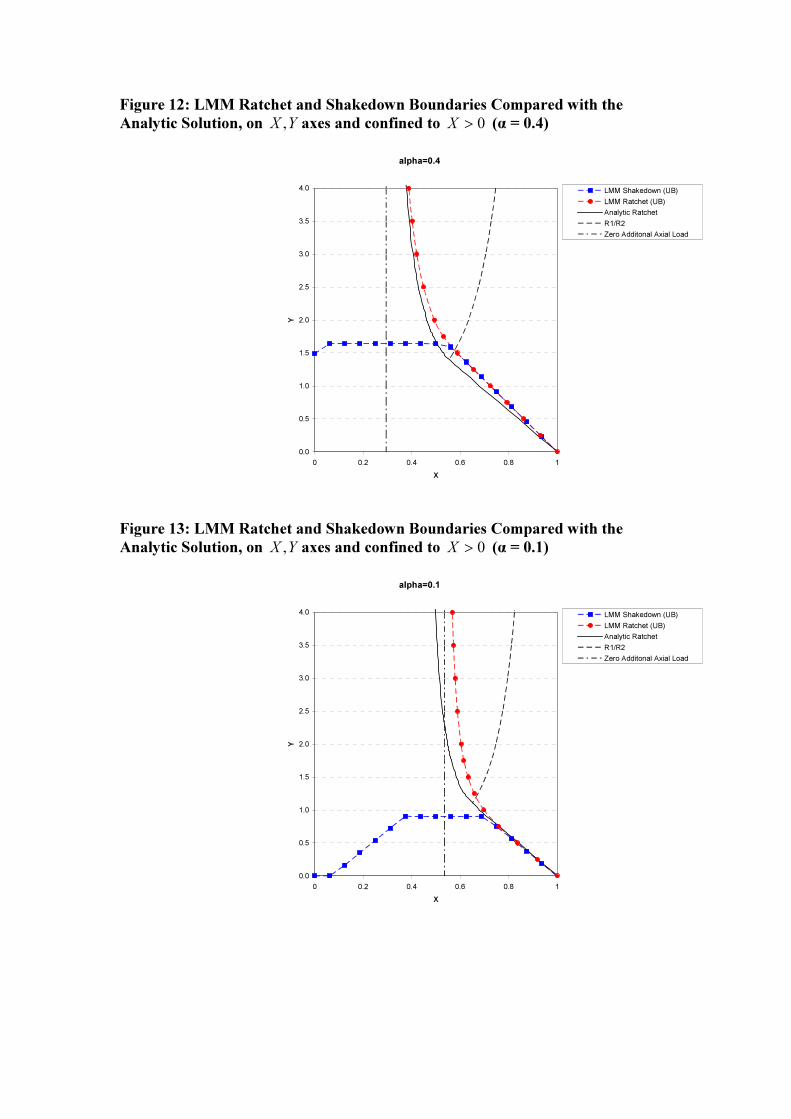
Figure 12: LMM Ratchet and Shakedown Boundaries Compared with the
Analytic Solution, on YX , axes and confined to 0>X (α = 0.4)
alpha=0.4
0.0
0.5
1.0
1.5
2.0
2.5
3.0
3.5
4.0
0 0.2 0.4 0.6 0.8 1
X
Y
LMM Shakedown (UB)
LMM Ratchet (UB)
Analytic Ratchet
R1/R2
Zero Additonal Axial Load
Figure 13: LMM Ratchet and Shakedown Boundaries Compared with the
Analytic Solution, on YX , axes and confined to 0>X (α = 0.1)
alpha=0.1
0.0
0.5
1.0
1.5
2.0
2.5
3.0
3.5
4.0
0 0.2 0.4 0.6 0.8 1
X
Y
LMM Shakedown (UB)
LMM Ratchet (UB)
Analytic Ratchet
R1/R2
Zero Additonal Axial Load
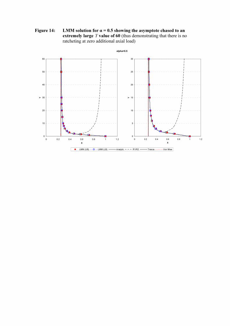
Figure 14: LMM solution for α = 0.5 showing the asymptote chased to an
extremely large Y value of 60 (thus demonstrating that there is no
ratcheting at zero additional axial load)
alpha=0.5
0
10
20
30
40
50
60
0 0.2 0.4 0.6 0.8 1 1.2
X
Y
LMM (UB) LMM (LB) Analytic R1/R2 Tresca Von Mise
0
5
10
15
20
25
30
0 0.2 0.4 0.6 0.8 1 1.2
X
Y


![Alan Jappy - pureportal.strath.ac.uk · Bree [1] showed that the shakedown and ratchet boundaries of a simplified representation of an internally pressurized pipe subjected to a thermal](https://img.pdfslide.us/doc/110x75/5e831de71be17b7cdc733d1e/alan-jappy-bree-1-showed-that-the-shakedown-and-ratchet-boundaries-of-a-simplified.jpg)