Embed Size (px)
Citation preview

The R Inferno
Patrick Burns1
30th April 2011
1This document resides in the tutorial section of http://www.burns-stat.com. Moreelementary material on R may also be found there. S+ is a registered trademark ofTIBCO Software Inc. The author thanks D. Alighieri for useful comments.
Contents
Contents 1
List of Figures 6
List of Tables 7
1 Falling into the Floating Point Trap 9
2 Growing Objects 12
3 Failing to Vectorize 173.1 Subscripting . . . . . . . . . . . . . . . . . . . . . . . . . . . . . . 203.2 Vectorized if . . . . . . . . . . . . . . . . . . . . . . . . . . . . . . 213.3 Vectorization impossible . . . . . . . . . . . . . . . . . . . . . . . 22
4 Over-Vectorizing 24
5 Not Writing Functions 275.1 Abstraction . . . . . . . . . . . . . . . . . . . . . . . . . . . . . . 275.2 Simplicity . . . . . . . . . . . . . . . . . . . . . . . . . . . . . . . 325.3 Consistency . . . . . . . . . . . . . . . . . . . . . . . . . . . . . . 33
6 Doing Global Assignments 35
7 Tripping on Object Orientation 387.1 S3 methods . . . . . . . . . . . . . . . . . . . . . . . . . . . . . . 38
7.1.1 generic functions . . . . . . . . . . . . . . . . . . . . . . . 397.1.2 methods . . . . . . . . . . . . . . . . . . . . . . . . . . . . 397.1.3 inheritance . . . . . . . . . . . . . . . . . . . . . . . . . . 40
7.2 S4 methods . . . . . . . . . . . . . . . . . . . . . . . . . . . . . . 407.2.1 multiple dispatch . . . . . . . . . . . . . . . . . . . . . . . 407.2.2 S4 structure . . . . . . . . . . . . . . . . . . . . . . . . . . 417.2.3 discussion . . . . . . . . . . . . . . . . . . . . . . . . . . . 42
7.3 Namespaces . . . . . . . . . . . . . . . . . . . . . . . . . . . . . . 42
1
CONTENTS CONTENTS
8 Believing It Does as Intended 448.1 Ghosts . . . . . . . . . . . . . . . . . . . . . . . . . . . . . . . . . 46
8.1.1 differences with S+ . . . . . . . . . . . . . . . . . . . . . . 468.1.2 package functionality . . . . . . . . . . . . . . . . . . . . . 468.1.3 precedence . . . . . . . . . . . . . . . . . . . . . . . . . . 478.1.4 equality of missing values . . . . . . . . . . . . . . . . . . 488.1.5 testing NULL . . . . . . . . . . . . . . . . . . . . . . . . . 488.1.6 membership . . . . . . . . . . . . . . . . . . . . . . . . . . 498.1.7 multiple tests . . . . . . . . . . . . . . . . . . . . . . . . . 498.1.8 coercion . . . . . . . . . . . . . . . . . . . . . . . . . . . . 508.1.9 comparison under coercion . . . . . . . . . . . . . . . . . 518.1.10 parentheses in the right places . . . . . . . . . . . . . . . 518.1.11 excluding named items . . . . . . . . . . . . . . . . . . . . 518.1.12 excluding missing values . . . . . . . . . . . . . . . . . . . 528.1.13 negative nothing is something . . . . . . . . . . . . . . . . 528.1.14 but zero can be nothing . . . . . . . . . . . . . . . . . . . 538.1.15 something plus nothing is nothing . . . . . . . . . . . . . 538.1.16 sum of nothing is zero . . . . . . . . . . . . . . . . . . . . 548.1.17 the methods shuffle . . . . . . . . . . . . . . . . . . . . . . 548.1.18 first match only . . . . . . . . . . . . . . . . . . . . . . . . 558.1.19 first match only (reprise) . . . . . . . . . . . . . . . . . . 558.1.20 partial matching can partially confuse . . . . . . . . . . . 568.1.21 no partial match assignments . . . . . . . . . . . . . . . . 588.1.22 cat versus print . . . . . . . . . . . . . . . . . . . . . . . . 588.1.23 backslashes . . . . . . . . . . . . . . . . . . . . . . . . . . 598.1.24 internationalization . . . . . . . . . . . . . . . . . . . . . . 598.1.25 paths in Windows . . . . . . . . . . . . . . . . . . . . . . 608.1.26 quotes . . . . . . . . . . . . . . . . . . . . . . . . . . . . . 608.1.27 backquotes . . . . . . . . . . . . . . . . . . . . . . . . . . 618.1.28 disappearing attributes . . . . . . . . . . . . . . . . . . . 628.1.29 disappearing attributes (reprise) . . . . . . . . . . . . . . 628.1.30 when space matters . . . . . . . . . . . . . . . . . . . . . 628.1.31 multiple comparisons . . . . . . . . . . . . . . . . . . . . . 638.1.32 name masking . . . . . . . . . . . . . . . . . . . . . . . . 638.1.33 more sorting than sort . . . . . . . . . . . . . . . . . . . . 638.1.34 sort.list not for lists . . . . . . . . . . . . . . . . . . . . . 648.1.35 search list shuffle . . . . . . . . . . . . . . . . . . . . . . . 648.1.36 source versus attach or load . . . . . . . . . . . . . . . . . 648.1.37 string not the name . . . . . . . . . . . . . . . . . . . . . 658.1.38 get a component . . . . . . . . . . . . . . . . . . . . . . . 658.1.39 string not the name (encore) . . . . . . . . . . . . . . . . 658.1.40 string not the name (yet again) . . . . . . . . . . . . . . . 658.1.41 string not the name (still) . . . . . . . . . . . . . . . . . . 668.1.42 name not the argument . . . . . . . . . . . . . . . . . . . 668.1.43 unexpected else . . . . . . . . . . . . . . . . . . . . . . . . 678.1.44 dropping dimensions . . . . . . . . . . . . . . . . . . . . . 67
2
CONTENTS CONTENTS
8.1.45 drop data frames . . . . . . . . . . . . . . . . . . . . . . . 688.1.46 losing row names . . . . . . . . . . . . . . . . . . . . . . . 688.1.47 apply function returning a vector . . . . . . . . . . . . . . 698.1.48 empty cells in tapply . . . . . . . . . . . . . . . . . . . . . 698.1.49 arithmetic that mixes matrices and vectors . . . . . . . . 708.1.50 single subscript of a data frame or array . . . . . . . . . . 718.1.51 non-numeric argument . . . . . . . . . . . . . . . . . . . . 718.1.52 round rounds to even . . . . . . . . . . . . . . . . . . . . 718.1.53 creating empty lists . . . . . . . . . . . . . . . . . . . . . 718.1.54 list subscripting . . . . . . . . . . . . . . . . . . . . . . . . 728.1.55 NULL or delete . . . . . . . . . . . . . . . . . . . . . . . . 738.1.56 disappearing components . . . . . . . . . . . . . . . . . . 738.1.57 combining lists . . . . . . . . . . . . . . . . . . . . . . . . 748.1.58 disappearing loop . . . . . . . . . . . . . . . . . . . . . . . 748.1.59 limited iteration . . . . . . . . . . . . . . . . . . . . . . . 748.1.60 too much iteration . . . . . . . . . . . . . . . . . . . . . . 758.1.61 wrong iterate . . . . . . . . . . . . . . . . . . . . . . . . . 758.1.62 wrong iterate (encore) . . . . . . . . . . . . . . . . . . . . 758.1.63 wrong iterate (yet again) . . . . . . . . . . . . . . . . . . 768.1.64 iterate is sacrosanct . . . . . . . . . . . . . . . . . . . . . 768.1.65 wrong sequence . . . . . . . . . . . . . . . . . . . . . . . . 768.1.66 empty string . . . . . . . . . . . . . . . . . . . . . . . . . 768.1.67 NA the string . . . . . . . . . . . . . . . . . . . . . . . . . 778.1.68 capitalization . . . . . . . . . . . . . . . . . . . . . . . . . 788.1.69 scoping . . . . . . . . . . . . . . . . . . . . . . . . . . . . 788.1.70 scoping (encore) . . . . . . . . . . . . . . . . . . . . . . . 78
8.2 Chimeras . . . . . . . . . . . . . . . . . . . . . . . . . . . . . . . 808.2.1 numeric to factor to numeric . . . . . . . . . . . . . . . . 828.2.2 cat factor . . . . . . . . . . . . . . . . . . . . . . . . . . . 828.2.3 numeric to factor accidentally . . . . . . . . . . . . . . . . 828.2.4 dropping factor levels . . . . . . . . . . . . . . . . . . . . 838.2.5 combining levels . . . . . . . . . . . . . . . . . . . . . . . 838.2.6 do not subscript with factors . . . . . . . . . . . . . . . . 848.2.7 no go for factors in ifelse . . . . . . . . . . . . . . . . . . . 848.2.8 no c for factors . . . . . . . . . . . . . . . . . . . . . . . . 848.2.9 ordering in ordered . . . . . . . . . . . . . . . . . . . . . . 858.2.10 labels and excluded levels . . . . . . . . . . . . . . . . . . 858.2.11 is missing missing or missing? . . . . . . . . . . . . . . . . 868.2.12 data frame to character . . . . . . . . . . . . . . . . . . . 878.2.13 nonexistent value in subscript . . . . . . . . . . . . . . . . 888.2.14 missing value in subscript . . . . . . . . . . . . . . . . . . 888.2.15 all missing subscripts . . . . . . . . . . . . . . . . . . . . . 898.2.16 missing value in if . . . . . . . . . . . . . . . . . . . . . . 908.2.17 and and andand . . . . . . . . . . . . . . . . . . . . . . . 908.2.18 equal and equalequal . . . . . . . . . . . . . . . . . . . . . 908.2.19 is.integer . . . . . . . . . . . . . . . . . . . . . . . . . . . 91
3
CONTENTS CONTENTS
8.2.20 is.numeric, as.numeric with integers . . . . . . . . . . . . 918.2.21 is.matrix . . . . . . . . . . . . . . . . . . . . . . . . . . . . 928.2.22 max versus pmax . . . . . . . . . . . . . . . . . . . . . . . 928.2.23 all.equal returns a surprising value . . . . . . . . . . . . . 938.2.24 all.equal is not identical . . . . . . . . . . . . . . . . . . . 938.2.25 identical really really means identical . . . . . . . . . . . . 938.2.26 = is not a synonym of <- . . . . . . . . . . . . . . . . . . 948.2.27 complex arithmetic . . . . . . . . . . . . . . . . . . . . . . 948.2.28 complex is not numeric . . . . . . . . . . . . . . . . . . . 948.2.29 nonstandard evaluation . . . . . . . . . . . . . . . . . . . 958.2.30 help for for . . . . . . . . . . . . . . . . . . . . . . . . . . 958.2.31 subset . . . . . . . . . . . . . . . . . . . . . . . . . . . . . 968.2.32 = vs == in subset . . . . . . . . . . . . . . . . . . . . . . 968.2.33 single sample switch . . . . . . . . . . . . . . . . . . . . . 968.2.34 changing names of pieces . . . . . . . . . . . . . . . . . . 978.2.35 a puzzle . . . . . . . . . . . . . . . . . . . . . . . . . . . . 978.2.36 another puzzle . . . . . . . . . . . . . . . . . . . . . . . . 988.2.37 data frames vs matrices . . . . . . . . . . . . . . . . . . . 988.2.38 apply not for data frames . . . . . . . . . . . . . . . . . . 988.2.39 data frames vs matrices (reprise) . . . . . . . . . . . . . . 988.2.40 names of data frames and matrices . . . . . . . . . . . . . 998.2.41 conflicting column names . . . . . . . . . . . . . . . . . . 998.2.42 cbind favors matrices . . . . . . . . . . . . . . . . . . . . . 1008.2.43 data frame equal number of rows . . . . . . . . . . . . . . 1008.2.44 matrices in data frames . . . . . . . . . . . . . . . . . . . 100
8.3 Devils . . . . . . . . . . . . . . . . . . . . . . . . . . . . . . . . . 1018.3.1 read.table . . . . . . . . . . . . . . . . . . . . . . . . . . . 1018.3.2 read a table . . . . . . . . . . . . . . . . . . . . . . . . . . 1018.3.3 the missing, the whole missing and nothing but the missing1028.3.4 misquoting . . . . . . . . . . . . . . . . . . . . . . . . . . 1028.3.5 thymine is TRUE, female is FALSE . . . . . . . . . . . . 1028.3.6 whitespace is white . . . . . . . . . . . . . . . . . . . . . . 1048.3.7 extraneous fields . . . . . . . . . . . . . . . . . . . . . . . 1048.3.8 fill and extraneous fields . . . . . . . . . . . . . . . . . . . 1048.3.9 reading messy files . . . . . . . . . . . . . . . . . . . . . . 1058.3.10 imperfection of writing then reading . . . . . . . . . . . . 1058.3.11 non-vectorized function in integrate . . . . . . . . . . . . 1058.3.12 non-vectorized function in outer . . . . . . . . . . . . . . 1068.3.13 ignoring errors . . . . . . . . . . . . . . . . . . . . . . . . 1068.3.14 accidentally global . . . . . . . . . . . . . . . . . . . . . . 1078.3.15 handling ... . . . . . . . . . . . . . . . . . . . . . . . . . . 1078.3.16 laziness . . . . . . . . . . . . . . . . . . . . . . . . . . . . 1088.3.17 lapply laziness . . . . . . . . . . . . . . . . . . . . . . . . 1088.3.18 invisibility cloak . . . . . . . . . . . . . . . . . . . . . . . 1098.3.19 evaluation of default arguments . . . . . . . . . . . . . . . 1098.3.20 sapply simplification . . . . . . . . . . . . . . . . . . . . . 110
4

CONTENTS CONTENTS
8.3.21 one-dimensional arrays . . . . . . . . . . . . . . . . . . . . 1108.3.22 by is for data frames . . . . . . . . . . . . . . . . . . . . . 1108.3.23 stray backquote . . . . . . . . . . . . . . . . . . . . . . . . 1118.3.24 array dimension calculation . . . . . . . . . . . . . . . . . 1118.3.25 replacing pieces of a matrix . . . . . . . . . . . . . . . . . 1118.3.26 reserved words . . . . . . . . . . . . . . . . . . . . . . . . 1128.3.27 return is a function . . . . . . . . . . . . . . . . . . . . . . 1128.3.28 return is a function (still) . . . . . . . . . . . . . . . . . . 1138.3.29 BATCH failure . . . . . . . . . . . . . . . . . . . . . . . . 1138.3.30 corrupted .RData . . . . . . . . . . . . . . . . . . . . . . . 1138.3.31 syntax errors . . . . . . . . . . . . . . . . . . . . . . . . . 1138.3.32 general confusion . . . . . . . . . . . . . . . . . . . . . . . 114
9 Unhelpfully Seeking Help 1159.1 Read the documentation . . . . . . . . . . . . . . . . . . . . . . . 1159.2 Check the FAQ . . . . . . . . . . . . . . . . . . . . . . . . . . . . 1169.3 Update . . . . . . . . . . . . . . . . . . . . . . . . . . . . . . . . 1169.4 Read the posting guide . . . . . . . . . . . . . . . . . . . . . . . . 1179.5 Select the best list . . . . . . . . . . . . . . . . . . . . . . . . . . 1179.6 Use a descriptive subject line . . . . . . . . . . . . . . . . . . . . 1189.7 Clearly state your question . . . . . . . . . . . . . . . . . . . . . 1189.8 Give a minimal example . . . . . . . . . . . . . . . . . . . . . . . 1209.9 Wait . . . . . . . . . . . . . . . . . . . . . . . . . . . . . . . . . . 121
Index 123
5
List of Figures
2.1 The giants by Sandro Botticelli. . . . . . . . . . . . . . . . . . . . 14
3.1 The hypocrites by Sandro Botticelli. . . . . . . . . . . . . . . . . 19
4.1 The panderers and seducers and the flatterers by Sandro Botticelli. 25
5.1 Stack of environments through time. . . . . . . . . . . . . . . . . 32
6.1 The sowers of discord by Sandro Botticelli. . . . . . . . . . . . . 36
7.1 The Simoniacs by Sandro Botticelli. . . . . . . . . . . . . . . . . 41
8.1 The falsifiers: alchemists by Sandro Botticelli. . . . . . . . . . . . 478.2 The treacherous to kin and the treacherous to country by Sandro
Botticelli. . . . . . . . . . . . . . . . . . . . . . . . . . . . . . . . 818.3 The treacherous to country and the treacherous to guests and
hosts by Sandro Botticelli. . . . . . . . . . . . . . . . . . . . . . . 103
9.1 The thieves by Sandro Botticelli. . . . . . . . . . . . . . . . . . . 1169.2 The thieves by Sandro Botticelli. . . . . . . . . . . . . . . . . . . 119
6

List of Tables
2.1 Time in seconds of methods to create a sequence. . . . . . . . . . 12
3.1 Summary of subscripting with 8 [ 8 . . . . . . . . . . . . . . . . . . 20
4.1 The apply family of functions. . . . . . . . . . . . . . . . . . . . . 24
5.1 Simple objects. . . . . . . . . . . . . . . . . . . . . . . . . . . . . 295.2 Some not so simple objects. . . . . . . . . . . . . . . . . . . . . . 29
8.1 A few of the most important backslashed characters. . . . . . . . 598.2 Functions to do with quotes. . . . . . . . . . . . . . . . . . . . . 61
7
Preface
Abstract: If you are using R and you think you’re in hell, this is a map foryou.
wandered through
http://www.r-project.org.
To state the good I found there, I’ll also say what else I saw.
Having abandoned the true way, I fell into a deep sleep and awoke in a deepdark wood. I set out to escape the wood, but my path was blocked by a lion.As I fled to lower ground, a figure appeared before me. “Have mercy on me,whatever you are,” I cried, “whether shade or living human.”
“Not a man, though once I was. My parents were from Lombardy. I wasborn sub Julio and lived in Rome in an age of false and lying gods.”
“Are you Virgil, the fountainhead of such a volume?”“I think it wise you follow me. I’ll lead you through an eternal place where
you shall hear despairing cries and see those ancient souls in pain as they grievetheir second death.”
After a journey, we arrived at an archway. Inscribed on it: “Through methe way into the suffering city, through me the way among the lost.” Throughthe archway we went.
Now sighing and wails resounded through the starless air, so that I toobegan weeping. Unfamiliar tongues, horrendous accents, cries of rage—all ofthese whirled in that dark and timeless air.
8

Circle 1
Falling into the FloatingPoint Trap
Once we had crossed the Acheron, we arrived in the first Circle, home of thevirtuous pagans. These are people who live in ignorance of the Floating PointGods. These pagans expect
.1 == .3 / 3
to be true.The virtuous pagans will also expect
seq(0, 1, by=.1) == .3
to have exactly one value that is true.But you should not expect something like:
unique(c(.3, .4 - .1, .5 - .2, .6 - .3, .7 - .4))
to have length one.
I wrote my first program in the late stone age. The task was to programthe quadratic equation. Late stone age means the medium of expression waspunchcards. There is no backspace on a punchcard machine—once the holesare there, there’s no filling them back in again. So a typo at the end of a linemeans that you have to throw the card out and start the line all over again. Aprocedure with which I became all too familiar.
Joy ensued at the end of the long ordeal of acquiring a pack of properlypunched cards. Short-lived joy. The next step was to put the stack of cardsinto an in-basket monitored by the computer operator. Some hours later the(large) paper output from the job would be in a pigeonhole. There was of coursean error in the program. After another struggle with the punchcard machine(relatively brief this time), the card deck was back in the in-basket.
9

CIRCLE 1. FALLING INTO THE FLOATING POINT TRAP
It didn’t take many iterations before I realized that it only ever told meabout the first error it came to. Finally on the third day, the output featuredno messages about errors. There was an answer—a wrong answer. It was asimple quadratic equation, and the answer was clearly 2 and 3. The programsaid it was 1.999997 and 3.000001. All those hours of misery and it can’t evenget the right answer.
I can write an R function for the quadratic formula somewhat quicker.
> quadratic.formula
function (a, b, c)
{rad <- b^2 - 4 * a * c
if(is.complex(rad) || all(rad >= 0)) {rad <- sqrt(rad)
} else {rad <- sqrt(as.complex(rad))
}cbind(-b - rad, -b + rad) / (2 * a)
}> quadratic.formula(1, -5, 6)
[,1] [,2]
[1,] 2 3
> quadratic.formula(1, c(-5, 1), 6)
[,1] [,2]
[1,] 2.0+0.000000i 3.0+0.000000i
[2,] -0.5-2.397916i -0.5+2.397916i
It is more general than that old program, and more to the point it gets theright answer of 2 and 3. Except that it doesn’t. R merely prints so that mostnumerical error is invisible. We can see how wrong it actually is by subtractingthe right answer:
> quadratic.formula(1, -5, 6) - c(2, 3)
[,1] [,2]
[1,] 0 0
Well okay, it gets the right answer in this case. But there is error if we changethe problem a little:
> quadratic.formula(1/3, -5/3, 6/3)
[,1] [,2]
[1,] 2 3
> print(quadratic.formula(1/3, -5/3, 6/3), digits=16) [,1] [,2]
[1,] 1.999999999999999 3.000000000000001
> quadratic.formula(1/3, -5/3, 6/3) - c(2, 3)
[,1] [,2]
[1,] -8.881784e-16 1.332268e-15
10

CIRCLE 1. FALLING INTO THE FLOATING POINT TRAP
That R prints answers nicely is a blessing. And a curse. R is good enough athiding numerical error that it is easy to forget that it is there. Don’t forget.
Whenever floating point operations are done—even simple ones, you shouldassume that there will be numerical error. If by chance there is no error, regardthat as a happy accident—not your due. You can use the all.equal functioninstead of 8 == 8 to test equality of floating point numbers.
If you have a case where the numbers are logically integer but they havebeen computed, then use round to make sure they really are integers.
Do not confuse numerical error with an error. An error is when a com-putation is wrongly performed. Numerical error is when there is visible noiseresulting from the finite representation of numbers. It is numerical error—notan error—when one-third is represented as 33%.
We’ve seen another aspect of virtuous pagan beliefs—what is printed is allthat there is.
> 7/13 - 3/31
[1] 0.4416873
R prints—by default—a handy abbreviation, not all that it knows about num-bers:
> print(7/13 - 3/31, digits=16)
[1] 0.4416873449131513
Many summary functions are even more restrictive in what they print:
> summary(7/13 - 3/31)
Min. 1st Qu. Median Mean 3rd Qu. Max.
0.4417 0.4417 0.4417 0.4417 0.4417 0.4417
Numerical error from finite arithmetic can not only fuzz the answer, it can fuzzthe question. In mathematics the rank of a matrix is some specific integer. Incomputing, the rank of a matrix is a vague concept. Since eigenvalues need notbe clearly zero or clearly nonzero, the rank need not be a definite number.
We descended to the edge of the first Circle where Minos stands guard,gnashing his teeth. The number of times he wraps his tail around himselfmarks the level of the sinner before him.
11

Circle 2
Growing Objects
We made our way into the second Circle, here live the gluttons.
Let’s look at three ways of doing the same task of creating a sequence ofnumbers. Method 1 is to grow the object:
vec <- numeric(0)
for(i in 1:n) vec <- c(vec, i)
Method 2 creates an object of the final length and then changes the values inthe object by subscripting:
vec <- numeric(n)
for(i in 1:n) vec[i] <- i
Method 3 directly creates the final object:
vec <- 1:n
Table 2.1 shows the timing in seconds on a particular (old) machine of thesethree methods for a selection of values of n. The relationships for varying n areall roughly linear on a log-log scale, but the timings are drastically different.
You may wonder why growing objects is so slow. It is the computationalequivalent of suburbanization. When a new size is required, there will not be
Table 2.1: Time in seconds of methods to create a sequence.
n grow subscript colon operator
1000 0.01 0.01 .0000610,000 0.59 0.09 .0004100,000 133.68 0.79 .005
1,000,000 18,718 8.10 .097
12

CIRCLE 2. GROWING OBJECTS
enough room where the object is; so it needs to move to a more open space.Then that space will be too small, and it will need to move again. It takes a lotof time to move house. Just as in physical suburbanization, growing objects canspoil all of the available space. You end up with lots of small pieces of availablememory, but no large pieces. This is called fragmenting memory.
A more common—and probably more dangerous—means of being a gluttonis with rbind. For example:
my.df <- data.frame(a=character(0), b=numeric(0))
for(i in 1:n) {my.df <- rbind(my.df, data.frame(a=sample(letters, 1),
b=runif(1)))
}Probably the main reason this is more common is because it is more likely thateach iteration will have a different number of observations. That is, the code ismore likely to look like:
my.df <- data.frame(a=character(0), b=numeric(0))
for(i in 1:n) {this.N <- rpois(1, 10)
my.df <- rbind(my.df, data.frame(a=sample(letters,
this.N, replace=TRUE), b=runif(this.N)))
}Often a reasonable upper bound on the size of the final object is known. If so,then create the object with that size and then remove the extra values at theend. If the final size is a mystery, then you can still follow the same scheme,but allow for periodic growth of the object.
current.N <- 10 * n
my.df <- data.frame(a=character(current.N),
b=numeric(current.N))
count <- 0
for(i in 1:n) {this.N <- rpois(1, 10)
if(count + this.N > current.N) {old.df <- my.df
current.N <- round(1.5 * (current.N + this.N))
my.df <- data.frame(a=character(current.N),
b=numeric(current.N))
my.df[1:count,] <- old.df[1:count, ]
}my.df[count + 1:this.N,] <- data.frame(a=sample(letters,
this.N, replace=TRUE), b=runif(this.N))
count <- count + this.N
}my.df <- my.df[1:count,]
13

CIRCLE 2. GROWING OBJECTS
Figure 2.1: The giants by Sandro Botticelli.
Often there is a simpler approach to the whole problem—build a list of piecesand then scrunch them together in one go.
my.list <- vector(’list’, n)
for(i in 1:n) {this.N <- rpois(1, 10)
my.list[[i]] <- data.frame(a=sample(letters, this.N
replace=TRUE), b=runif(this.N))
}my.df <- do.call(’rbind’, my.list)
There are ways of cleverly hiding that you are growing an object. Here is anexample:
hit <- NA
for(i in 1:one.zillion) {if(runif(1) < 0.3) hit[i] <- TRUE
}
Each time the condition is true, hit is grown.Eliminating the growth of objects can be one of the easiest and most dra-
matic ways of speeding up R code.
14
CIRCLE 2. GROWING OBJECTS
If you use too much memory, R will complain. The key issue is that R holdsall the data in RAM. This is a limitation if you have huge datasets. The up-sideis flexibility—in particular, R imposes no rules on what data are like.
You can get a message, all too familiar to some people, like:
Error: cannot allocate vector of size 79.8 Mb.
This is often misinterpreted along the lines of: “I have xxx gigabytes of memory,why can’t R even allocate 80 megabytes?” It is because R has already allocateda lot of memory successfully. The error message is about how much memory Rwas going after at the point where it failed.
The user who has seen this message logically asks, “What can I do aboutit?” There are some easy answers:
1. Don’t be a glutton by using bad programming constructs.
2. Get a bigger computer.
3. Reduce the problem size.
If you’ve obeyed the first answer and can’t follow the second or third, thenyour alternatives are harder. One is to restart the R session, but this is oftenineffective.
Another of those hard alternatives is to explore where in your code thememory is growing. One method (on at least one platform) is to insert lineslike:
cat(’point 1 mem’, memory.size(), memory.size(max=TRUE), ’\n’)
throughout your code. This shows the memory that R currently has and themaximum amount R has had in the current session.
However, probably a more efficient and informative procedure would be touse Rprof with memory profiling. Rprof also profiles time use.
Another way of reducing memory use is to store your data in a database andonly extract portions of the data into R as needed. While this takes some timeto set up, it can become quite a natural way to work.
A “database” solution that only uses R is to save (as in the save function)objects in individual files, then use the files one at a time. So your code usingthe objects might look something like:
for(i in 1:n) {objname <- paste(’obj.’, i, sep=’’)
load(paste(objname, ’.rda’, sep=’’))
the obj <- get(objname)
rm(list=objname)
# use the obj
}
15
CIRCLE 2. GROWING OBJECTS
Are tomorrow’s bigger computers going to solve the problem? For some people,yes—their data will stay the same size and computers will get big enough tohold it comfortably. For other people it will only get worse—more powerfulcomputers means extraordinarily larger datasets. If you are likely to be in thislatter group, you might want to get used to working with databases now.
If you have one of those giant computers, you may have the capacity toattempt to create something larger than R can handle. See:
?’Memory-limits’
for the limits that are imposed.
16
Circle 3
Failing to Vectorize
We arrive at the third Circle, filled with cold, unending rain. Here standsCerberus barking out of his three throats. Within the Circle were the blas-phemous wearing golden, dazzling cloaks that inside were all of lead—weighingthem down for all of eternity. This is where Virgil said to me, “Remember yourscience—the more perfect a thing, the more its pain or pleasure.”
Here is some sample code:
lsum <- 0
for(i in 1:length(x)) {lsum <- lsum + log(x[i])
}
No. No. No.This is speaking R with a C accent—a strong accent. We can do the same
thing much simpler:
lsum <- sum(log(x))
This is not only nicer for your carpal tunnel, it is computationally much faster.(As an added bonus it avoids the bug in the loop when x has length zero.)
The command above works because of vectorization. The log function isvectorized in the traditional sense—it does the same operation on a vector ofvalues as it would do on each single value. That is, the command:
log(c(23, 67.1))
has the same result as the command:
c(log(23), log(67.1))
The sum function is vectorized in a quite different sense—it takes a vector andproduces something based on the whole vector. The command sum(x) is equiv-alent to:
17

CIRCLE 3. FAILING TO VECTORIZE
x[1] + x[2] + ... + x[length(x)]
The prod function is similar to sum, but does products rather than sums. Prod-ucts can often overflow or underflow (a suburb of Circle 1)—taking logs anddoing sums is generally a more stable computation.
You often get vectorization for free. Take the example of quadratic.formulain Circle 1 (page 9). Since the arithmetic operators are vectorized, the result ofthis function is a vector if any or all of the inputs are. The only slight problemis that there are two answers per input, so the call to cbind is used to keeptrack of the pairs of answers.
In binary operations such as:
c(1,4) + 1:10
recycling automatically happens along with the vectorization.
Here is some code that combines both this Circle and Circle 2 (page 12):
ans <- NULL
for(i in 1:507980) {if(x[i] < 0) ans <- c(ans, y[i])
}
This can be done simply with:
ans <- y[x < 0]
A double for loop is often the result of a function that has been directly trans-lated from another language. Translations that are essentially verbatim areunlikely to be the best thing to do. Better is to rethink what is happening withR in mind. Using direct translations from another language may well leave youlonging for that other language. Making good translations may well leave youmarvelling at R’s strengths. (The catch is that you need to know the strengthsin order to make the good translations.)
If you are translating code into R that has a double for loop, think.
If your function is not vectorized, then you can possibly use the Vectorize
function to make a vectorized version. But this is vectorization from an externalpoint of view—it is not the same as writing inherently vectorized code. TheVectorize function performs a loop using the original function.
Some functions take a function as an argument and demand that the functionbe vectorized—these include outer and integrate.
There is another form of vectorization:
> max(2, 100, -4, 3, 230, 5)
[1] 230
> range(2, 100, -4, 3, 230, 5, c(4, -456, 9))
[1] -456 230
18

CIRCLE 3. FAILING TO VECTORIZE
Figure 3.1: The hypocrites by Sandro Botticelli.
This form of vectorization is to treat the collection of arguments as the vector.This is NOT a form of vectorization you should expect, it is essentially foreign toR—min, max, range, sum and prod are rare exceptions. In particular, mean doesnot adhere to this form of vectorization, and unfortunately does not generatean error from trying it:
> mean(2, -100, -4, 3, -230, 5)
[1] 2
But you get the correct answer if you add three (particular) keystrokes:
> mean(c(2, -100, -4, 3, -230, 5))
[1] -54
One reason for vectorization is for computational speed. In a vector operationthere is always a loop. If the loop is done in C code, then it will be much fasterthan if it is done in R code. In some cases, this can be very important. Inother cases, it isn’t—a loop in R code now is as fast as the same loop in C ona computer from a few years ago.
Another reason to vectorize is for clarity. The command:
volume <- width * depth * height
19
3.1. SUBSCRIPTING CIRCLE 3. FAILING TO VECTORIZE
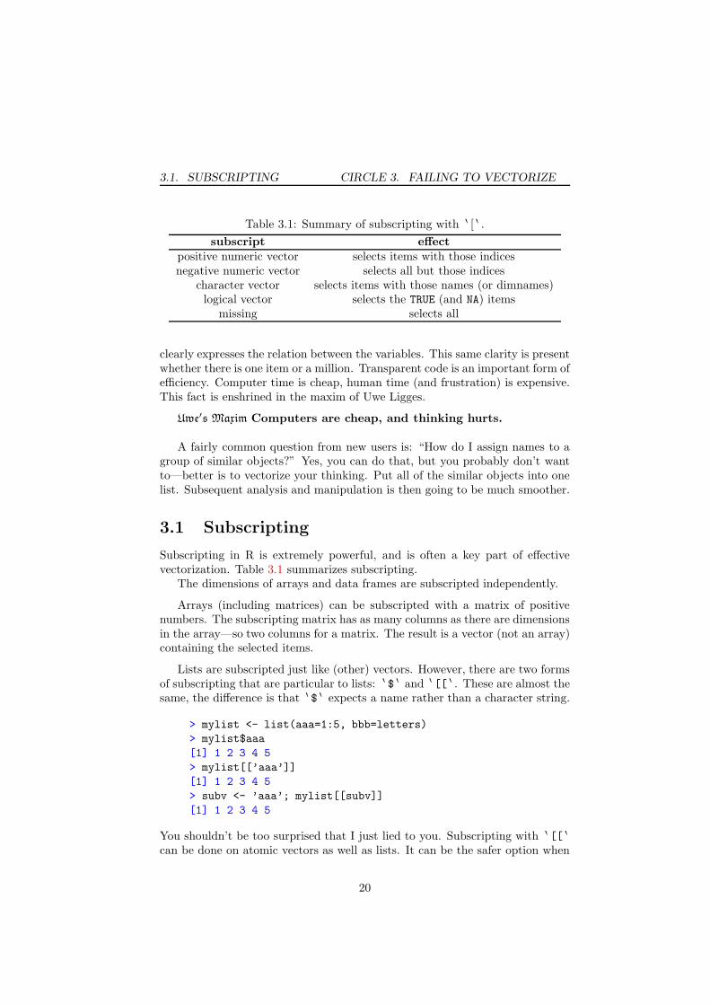
Table 3.1: Summary of subscripting with 8 [ 8 .
subscript effectpositive numeric vector selects items with those indicesnegative numeric vector selects all but those indices
character vector selects items with those names (or dimnames)logical vector selects the TRUE (and NA) items
missing selects all
clearly expresses the relation between the variables. This same clarity is presentwhether there is one item or a million. Transparent code is an important form ofefficiency. Computer time is cheap, human time (and frustration) is expensive.This fact is enshrined in the maxim of Uwe Ligges.
Uwe′s Maxim Computers are cheap, and thinking hurts.
A fairly common question from new users is: “How do I assign names to agroup of similar objects?” Yes, you can do that, but you probably don’t wantto—better is to vectorize your thinking. Put all of the similar objects into onelist. Subsequent analysis and manipulation is then going to be much smoother.
3.1 Subscripting
Subscripting in R is extremely powerful, and is often a key part of effectivevectorization. Table 3.1 summarizes subscripting.
The dimensions of arrays and data frames are subscripted independently.
Arrays (including matrices) can be subscripted with a matrix of positivenumbers. The subscripting matrix has as many columns as there are dimensionsin the array—so two columns for a matrix. The result is a vector (not an array)containing the selected items.
Lists are subscripted just like (other) vectors. However, there are two formsof subscripting that are particular to lists: 8 $ 8 and 8 [[ 8 . These are almost thesame, the difference is that 8 $ 8 expects a name rather than a character string.
> mylist <- list(aaa=1:5, bbb=letters)
> mylist$aaa
[1] 1 2 3 4 5
> mylist[[’aaa’]]
[1] 1 2 3 4 5
> subv <- ’aaa’; mylist[[subv]]
[1] 1 2 3 4 5
You shouldn’t be too surprised that I just lied to you. Subscripting with 8 [[ 8
can be done on atomic vectors as well as lists. It can be the safer option when
20

3.2. VECTORIZED IF CIRCLE 3. FAILING TO VECTORIZE
a single item is demanded. If you are using 8 [[ 8 and you want more than oneitem, you are going to be disappointed.
We’ve already seen (in the lsum example) that subscripting can be a symp-tom of not vectorizing.
As an example of how subscripting can be a vectorization tool, considerthe following problem: We have a matrix amat and we want to produce a newmatrix with half as many rows where each row of the new matrix is the productof two consecutive rows of amat.
It is quite simple to create a loop to do this:
bmat <- matrix(NA, nrow(amat)/2, ncol(amat))
for(i in 1:nrow(bmat)) bmat[i,] <- amat[2*i-1,] * amat[2*i,]
Note that we have avoided Circle 2 (page 12) by preallocating bmat.Later iterations do not depend on earlier ones, so there is hope that we can
eliminate the loop. Subscripting is the key to the elimination:
> bmat2 <- amat[seq(1, nrow(amat), by=2),] *
+ amat[seq(2, nrow(amat), by=2),]
> all.equal(bmat, bmat2)
[1] TRUE
3.2 Vectorized if
Here is some code:
if(x < 1) y <- -1 else y <- 1
This looks perfectly logical. And if x has length one, then it does as expected.However, if x has length greater than one, then a warning is issued (often ignoredby the user), and the result is not what is most likely intended. Code that fulfillsthe common expectation is:
y <- ifelse(x < 1, -1, 1)
Another approach—assuming x is never exactly 1—is:
y <- sign(x - 1)
This provides a couple of lessons:
1. The condition in if is one of the few places in R where a vector (of lengthgreater than 1) is not welcome (the 8 : 8 operator is another).
2. ifelse is what you want in such a situation (though, as in this case, thereare often more direct approaches).
21

3.3. VEC IMPOSSIBLE CIRCLE 3. FAILING TO VECTORIZE
Recall that in Circle 2 (page 12) we saw:
hit <- NA
for(i in 1:one.zillion) {if(runif(1) < 0.3) hit[i] <- TRUE
}
One alternative to make this operation efficient is:
ifelse(runif(one.zillion) < 0.3, TRUE, NA)
If there is a mistake between if and ifelse, it is almost always trying to useif when ifelse is appropriate. But ingenuity knows no bounds, so it is alsopossible to try to use ifelse when if is appropriate. For example:
ifelse(x, character(0), ’’)
The result of ifelse is ALWAYS the length of its first (formal) argument.Assuming that x is of length 1, the way to get the intended behavior is:
if(x) character(0) else ’’
Some more caution is warranted with ifelse: the result gets not only its lengthfrom the first argument, but also its attributes. If you would like the answerto have attributes of the other two arguments, you need to do more work. InCircle 8.2.7 we’ll see a particular instance of this with factors.
3.3 Vectorization impossible
Some things are not possible to vectorize. For instance, if the present iterationdepends on results from the previous iteration, then vectorization is usually notpossible. (But some cases are covered by filter, cumsum, etc.)
If you need to use a loop, then make it lean:
• Put as much outside of loops as possible. One example: if the same or asimilar sequence is created in each iteration, then create the sequence firstand reuse it. Creating a sequence is quite fast, but appreciable time canaccumulate if it is done thousands or millions of times.
• Make the number of iterations as small as possible. If you have the choiceof iterating over the elements of a factor or iterating over the levels of thefactor, then iterating over the levels is going to be better (almost surely).
The following bit of code gets the sum of each column of a matrix (assumingthe number of columns is positive):
sumxcol <- numeric(ncol(x))
for(i in 1:ncol(x)) sumxcol[i] <- sum(x[,i])
22

3.3. VEC IMPOSSIBLE CIRCLE 3. FAILING TO VECTORIZE
A more common approach to this would be:
sumxcol <- apply(x, 2, sum)
Since this is a quite common operation, there is a special function for doing thisthat does not involve a loop in R code:
sumxcol <- colSums(x)
There are also rowSums, colMeans and rowMeans.Another approach is:
sumxcol <- rep(1, nrow(x)) %*% x
That is, using matrix multiplication. With a little ingenuity a lot of problemscan be cast into a matrix multiplication form. This is generally quite efficientrelative to alternatives.
23

Circle 4
Over-Vectorizing
We skirted past Plutus, the fierce wolf with a swollen face, down into the fourthCircle. Here we found the lustful.
It is a good thing to want to vectorize when there is no effective way to doso. It is a bad thing to attempt it anyway.
A common reflex is to use a function in the apply family. This is not vector-ization, it is loop-hiding. The apply function has a for loop in its definition.The lapply function buries the loop, but execution times tend to be roughlyequal to an explicit for loop. (Confusion over this is understandable, as thereis a significant difference in execution speed with at least some versions of S+.)Table 4.1 summarizes the uses of the apply family of functions.
Base your decision of using an apply function on Uwe’s Maxim (page 20).The issue is of human time rather than silicon chip time. Human time can bewasted by taking longer to write the code, and (often much more importantly)by taking more time to understand subsequently what it does.
A command applying a complicated function is unlikely to pass the test.
Table 4.1: The apply family of functions.
function input output commentapply matrix or array vector or array or listlapply list or vector listsapply list or vector vector or matrix or list simplifyvapply list or vector vector or matrix or list safer simplifytapply data, categories array or list raggedmapply lists and/or vectors vector or matrix or list multiplerapply list vector or list recursiveeapply environment list
dendrapply dendogram dendogramrollapply data similar to input package zoo
24
CIRCLE 4. OVER-VECTORIZING
Figure 4.1: The panderers and seducers and the flatterers by Sandro Botticelli.
Use an explicit for loop when each iteration is a non-trivial task. But a simpleloop can be more clearly and compactly expressed using an apply function.
There is at least one exception to this rule. We will see in Circle 8.1.56 thatif the result will be a list and some of the components can be NULL, then a for
loop is trouble (big trouble) and lapply gives the expected answer.
The tapply function applies a function to each bit of a partition of the data.Alternatives to tapply are by for data frames, and aggregate for time seriesand data frames. If you have a substantial amount of data and speed is an issue,then data.table may be a good solution.
Another approach to over-vectorizing is to use too much memory in the pro-cess. The outer function is a wonderful mechanism to vectorize some problems.It is also subject to using a lot of memory in the process.
Suppose that we want to find all of the sets of three positive integers thatsum to 6, where the order matters. (This is related to partitions in numbertheory.) We can use outer and which:
the.seq <- 1:4
which(outer(outer(the.seq, the.seq, ’+’), the.seq, ’+’) == 6,
arr.ind=TRUE)
This command is nicely vectorized, and a reasonable solution to this particular
25

CIRCLE 4. OVER-VECTORIZING
problem. However, with larger problems this could easily eat all memory on amachine.
Suppose we have a data frame and we want to change the missing values tozero. Then we can do that in a perfectly vectorized manner:
x[is.na(x)] <- 0
But if x is large, then this may take a lot of memory. If—as is common—thenumber of rows is much larger than the number of columns, then a more memoryefficient method is:
for(i in 1:ncol(x)) x[is.na(x[,i]), i] <- 0
Note that “large” is a relative term; it is usefully relative to the amount ofavailable memory on your machine. Also note that memory efficiency can alsobe time efficiency if the inefficient approach causes swapping.
One more comment: if you really want to change NAs to 0, perhaps youshould rethink what you are doing—the new data are fictional.
It is not unusual for there to be a tradeoff between space and time.
Beware the dangers of premature optimization of your code. Your first dutyis to create clear, correct code. Only consider optimizing your code when:
• Your code is debugged and stable.
• Optimization is likely to make a significant impact. Spending an hour ortwo to save a millisecond a month is not best practice.
26

Circle 5
Not Writing Functions
We came upon the River Styx, more a swamp really. It took some convinc-ing, but Phlegyas eventually rowed us across in his boat. Here we found thetreasoners.
5.1 Abstraction
A key reason that R is a good thing is because it is a language. The power oflanguage is abstraction. The way to make abstractions in R is to write functions.
Suppose we want to repeat the integers 1 through 3 twice. That’s a simplecommand:
c(1:3, 1:3)
Now suppose we want these numbers repeated six times, or maybe sixty times.Writing a function that abstracts this operation begins to make sense. In fact,that abstraction has already been done for us:
rep(1:3, 6)
The rep function performs our desired task and a number of similar tasks.Let’s do a new task. We have two vectors; we want to produce a single vector
consisting of the first vector repeated to the length of the second and then thesecond vector repeated to the length of the first. A vector being repeated to ashorter length means to just use the first part of the vector. This is quite easilyabstracted into a function that uses rep:
repeat.xy <- function(x, y)
{c(rep(x, length=length(y)), rep(y, length=length(x)))
}
The repeat.xy function can now be used in the same way as if it came with R.
27

5.1. ABSTRACTION CIRCLE 5. NOT WRITING FUNCTIONS
repeat.xy(1:4, 6:16)
The ease of writing a function like this means that it is quite natural to movegradually from just using R to programming in R.
In addition to abstraction, functions crystallize knowledge. That π is approx-imately 3.1415926535897932384626433832795028841971693993751058209749445923078 is knowledge.
The function:
circle.area <- function(r) pi * r ^ 2
is both knowledge and abstraction—it gives you the (approximate) area forwhatever circles you like.
This is not the place for a full discussion on the structure of the R language,but a comment on a detail of the two functions that we’ve just created is inorder. The statement in the body of repeat.xy is surrounded by curly braceswhile the statement in the body of circle.area is not. The body of a functionneeds to be a single expression. Curly braces turn a number of expressions intoa single (combined) expression. When there is only a single command in thebody of a function, then the curly braces are optional. Curly braces are alsouseful with loops, switch and if.
Ideally each function performs a clearly specified task with easily understoodinputs and return value. Very common novice behavior is to write one functionthat does everything. Almost always a better approach is to write a number ofsmaller functions, and then a function that does everything by using the smallerfunctions. Breaking the task into steps often has the benefit of making it moreclear what really should be done. It is also much easier to debug when thingsgo wrong.1 The small functions are much more likely to be of general use.
A nice piece of abstraction in R functions is default values for arguments.For example, the na.rm argument to sd has a default value of FALSE. If thatis okay in a particular instance, then you don’t have to specify na.rm in yourcall. If you want to remove missing values, then you should include na.rm=TRUE
as an argument in your call. If you create your own copy of a function just tochange the default value of an argument, then you’re probably not appreciatingthe abstraction that the function gives you.
Functions return a value. The return value of a function is almost alwaysthe reason for the function’s existence. The last item in a function definitionis returned. Most functions merely rely on this mechanism, but the return
function forces what to return.The other thing that a function can do is to have one or more side effects.
A side effect is some change to the system other than returning a value. Thephilosophy of R is to concentrate side effects into a few functions (such as print,plot and rm) where it is clear that a side effect is to be expected.
1Notice “when” not “if”.
28
5.1. ABSTRACTION CIRCLE 5. NOT WRITING FUNCTIONS
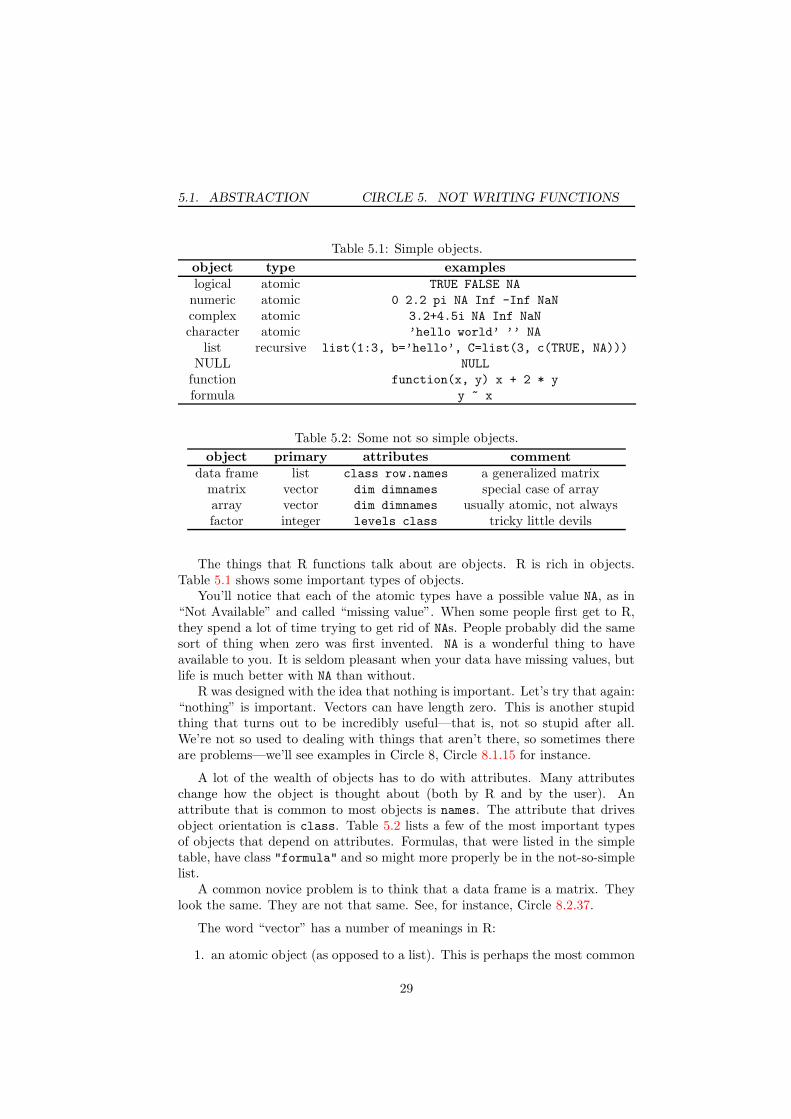
Table 5.1: Simple objects.
object type exampleslogical atomic TRUE FALSE NA
numeric atomic 0 2.2 pi NA Inf -Inf NaN
complex atomic 3.2+4.5i NA Inf NaN
character atomic ’hello world’ ’’ NA
list recursive list(1:3, b=’hello’, C=list(3, c(TRUE, NA)))
NULL NULL
function function(x, y) x + 2 * y
formula y ~ x
Table 5.2: Some not so simple objects.
object primary attributes commentdata frame list class row.names a generalized matrix
matrix vector dim dimnames special case of arrayarray vector dim dimnames usually atomic, not alwaysfactor integer levels class tricky little devils
The things that R functions talk about are objects. R is rich in objects.Table 5.1 shows some important types of objects.
You’ll notice that each of the atomic types have a possible value NA, as in“Not Available” and called “missing value”. When some people first get to R,they spend a lot of time trying to get rid of NAs. People probably did the samesort of thing when zero was first invented. NA is a wonderful thing to haveavailable to you. It is seldom pleasant when your data have missing values, butlife is much better with NA than without.
R was designed with the idea that nothing is important. Let’s try that again:“nothing” is important. Vectors can have length zero. This is another stupidthing that turns out to be incredibly useful—that is, not so stupid after all.We’re not so used to dealing with things that aren’t there, so sometimes thereare problems—we’ll see examples in Circle 8, Circle 8.1.15 for instance.
A lot of the wealth of objects has to do with attributes. Many attributeschange how the object is thought about (both by R and by the user). Anattribute that is common to most objects is names. The attribute that drivesobject orientation is class. Table 5.2 lists a few of the most important typesof objects that depend on attributes. Formulas, that were listed in the simpletable, have class "formula" and so might more properly be in the not-so-simplelist.
A common novice problem is to think that a data frame is a matrix. Theylook the same. They are not that same. See, for instance, Circle 8.2.37.
The word “vector” has a number of meanings in R:
1. an atomic object (as opposed to a list). This is perhaps the most common
29

5.1. ABSTRACTION CIRCLE 5. NOT WRITING FUNCTIONS
usage.
2. an object with no attributes (except possibly names). This is the definitionimplied by is.vector and as.vector.
3. an object that can have an arbitrary length (includes lists).
Clearly definitions 1 and 3 are contradictory, but which meaning is impliedshould be clear from the context. When the discussion is of vectors as opposedto matrices, it is definition 2 that is implied.
The word “list” has a technical meaning in R—this is an object of arbitrarylength that can have components of different types, including lists. Sometimesthe word is used in a non-technical sense, as in “search list” or “argument list”.
Not all functions are created equal. They can be conveniently put into threetypes.
There are anonymous functions as in:
apply(x, 2, function(z) mean(z[z > 0]))
The function given as the third argument to apply is so transient that we don’teven give it a name.
There are functions that are useful only for one particular project. Theseare your one-off functions.
Finally there are functions that are persistently valuable. Some of thesecould well be one-off functions that you have rewritten to be more abstract.You will most likely want a file or package containing your persistently usefulfunctions.
In the example of an anonymous function we saw that a function can be anargument to another function. In R, functions are objects just as vectors ormatrices are objects. You are allowed to think of functions as data.
A whole new level of abstraction is a function that returns a function. Theempirical cumulative distribution function is an example:
> mycumfun <- ecdf(rnorm(10))
> mycumfun(0)
[1] 0.4
Once you write a function that returns a function, you will be forever immuneto this Circle.
In Circle 2 (page 12) we briefly met do.call. Some people are quite confusedby do.call. That is both unnecessary and unfortunate—it is actually quitesimple and is very powerful. Normally a function is called by following thename of the function with an argument list:
sample(x=10, size=5)
30

5.1. ABSTRACTION CIRCLE 5. NOT WRITING FUNCTIONS
The do.call function allows you to provide the arguments as an actual list:
do.call("sample", list(x=10, size=5))
Simple.
At times it is useful to have an image of what happens when you call afunction. An environment is created by the function call, and an environmentis created for each function that is called by that function. So there is a stackof environments that grows and shrinks as the computation proceeds.
Let’s define some functions:
ftop <- function(x)
{# time 1
x1 <- f1(x)
# time 5
ans.top <- f2(x1)
# time 9
ans.top
}f1 <- function(x)
{# time 2
ans1 <- f1.1(x)
# time 4
ans1
}f2 <- function(x)
{# time 6
ans2 <- f2.1(x)
# time 8
ans2
}And now let’s do a call:
# time 0
ftop(myx)
# time 10
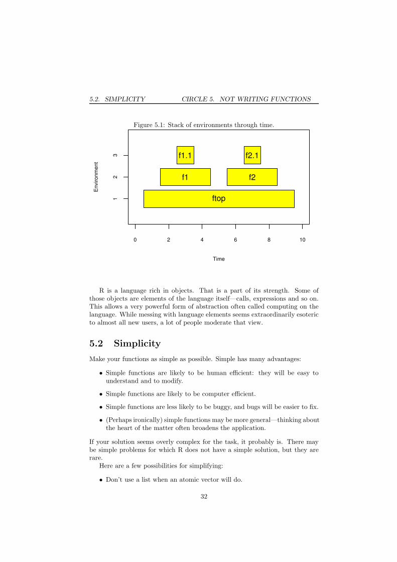
Figure 5.1 shows how the stack of environments for this call changes throughtime. Note that there is an x in the environments for ftop, f1 and f2. The x
in ftop is what we call myx (or possibly a copy of it) as is the x in f1. But thex in f2 is something different.
When we discuss debugging, we’ll be looking at this stack at a specific pointin time. For instance, if an error occurred in f2.1, then we would be looking atthe state of the stack somewhere near time 7.
31
5.2. SIMPLICITY CIRCLE 5. NOT WRITING FUNCTIONS
Figure 5.1: Stack of environments through time.
Time
Env
ironm
ent
0 2 4 6 8 10
12
3
ftop
f1 f2
f1.1 f2.1
R is a language rich in objects. That is a part of its strength. Some ofthose objects are elements of the language itself—calls, expressions and so on.This allows a very powerful form of abstraction often called computing on thelanguage. While messing with language elements seems extraordinarily esotericto almost all new users, a lot of people moderate that view.
5.2 Simplicity
Make your functions as simple as possible. Simple has many advantages:
• Simple functions are likely to be human efficient: they will be easy tounderstand and to modify.
• Simple functions are likely to be computer efficient.
• Simple functions are less likely to be buggy, and bugs will be easier to fix.
• (Perhaps ironically) simple functions may be more general—thinking aboutthe heart of the matter often broadens the application.
If your solution seems overly complex for the task, it probably is. There maybe simple problems for which R does not have a simple solution, but they arerare.
Here are a few possibilities for simplifying:
• Don’t use a list when an atomic vector will do.
32

5.3. CONSISTENCY CIRCLE 5. NOT WRITING FUNCTIONS
• Don’t use a data frame when a matrix will do.
• Don’t try to use an atomic vector when a list is needed.
• Don’t try to use a matrix when a data frame is needed.
Properly formatting your functions when you write them should be standardpractice. Here “proper” includes indenting based on the logical structure, andputting spaces between operators. Circle 8.1.30 shows that there is a particularlygood reason to put spaces around logical operators.
A semicolon can be used to mark the separation of two R commands thatare placed on the same line. Some people like to put semicolons at the end ofall lines. This highly annoys many seasoned R users. Such a reaction seems tobe more visceral than logical, but there is some logic to it:
• The superfluous semicolons create some (imperceptible) inefficiency.
• The superfluous semicolons give the false impression that they are doingsomething.
One reason to seek simplicity is speed. The Rprof function is a very convenientmeans of exploring which functions are using the most time in your functioncalls. (The name Rprof refers to time profiling.)
5.3 Consistency
Consistency is good. Consistency reduces the work that your users need toexpend. Consistency reduces bugs.
One form of consistency is the order and names of function arguments. Sur-prising your users is not a good idea—even if the universe of your users is ofsize 1.
A rather nice piece of consistency is always giving the correct answer. Inorder for that to happen the inputs need to be suitable. To insure that, thefunction needs to check inputs, and possibly intermediate results. The tools forthis job include if, stop and stopifnot.
Sometimes an occurrence is suspicious but not necessarily wrong. In thiscase a warning is appropriate. A warning produces a message but does notinterrupt the computation.
There is a problem with warnings. No one reads them. People have to readerror messages because no food pellet falls into the tray after they push thebutton. With a warning the machine merely beeps at them but they still gettheir food pellet. Never mind that it might be poison.
The appropriate reaction to a warning message is:
1. Figure out what the warning is saying.
33
5.3. CONSISTENCY CIRCLE 5. NOT WRITING FUNCTIONS
2. Figure out why the warning is triggered.
3. Figure out the effect on the results of the computation (via deduction orexperimentation).
4. Given the result of step 3, decide whether or not the results will be erro-neous.
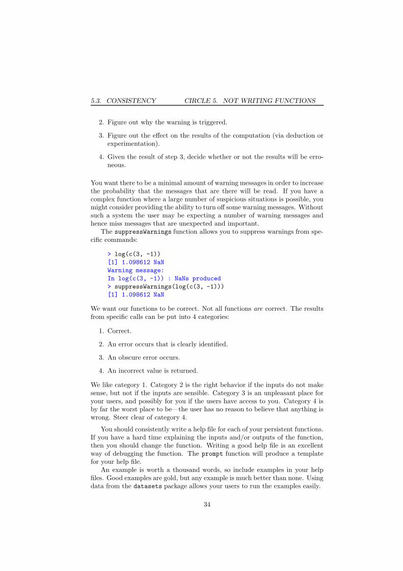
You want there to be a minimal amount of warning messages in order to increasethe probability that the messages that are there will be read. If you have acomplex function where a large number of suspicious situations is possible, youmight consider providing the ability to turn off some warning messages. Withoutsuch a system the user may be expecting a number of warning messages andhence miss messages that are unexpected and important.
The suppressWarnings function allows you to suppress warnings from spe-cific commands:
> log(c(3, -1))
[1] 1.098612 NaN
Warning message:
In log(c(3, -1)) : NaNs produced
> suppressWarnings(log(c(3, -1)))
[1] 1.098612 NaN
We want our functions to be correct. Not all functions are correct. The resultsfrom specific calls can be put into 4 categories:
1. Correct.
2. An error occurs that is clearly identified.
3. An obscure error occurs.
4. An incorrect value is returned.
We like category 1. Category 2 is the right behavior if the inputs do not makesense, but not if the inputs are sensible. Category 3 is an unpleasant place foryour users, and possibly for you if the users have access to you. Category 4 isby far the worst place to be—the user has no reason to believe that anything iswrong. Steer clear of category 4.
You should consistently write a help file for each of your persistent functions.If you have a hard time explaining the inputs and/or outputs of the function,then you should change the function. Writing a good help file is an excellentway of debugging the function. The prompt function will produce a templatefor your help file.
An example is worth a thousand words, so include examples in your helpfiles. Good examples are gold, but any example is much better than none. Usingdata from the datasets package allows your users to run the examples easily.
34
Circle 6
Doing Global Assignments
Heretics imprisoned in flaming tombs inhabit Circle 6.
A global assignment can be performed with 8 <<- 8 :
> x <- 1
> y <- 2
> fun
function () {x <- 101
y <<- 102
}> fun()
> x
[1] 1
> y
[1] 102
This is life beside a volcano.
If you think you need 8 <<- 8 , think again. If on reflection you still think youneed 8 <<- 8 , think again. Only when your boss turns red with anger over younot doing anything should you temporarily give in to the temptation. Therehave been proposals (no more than half-joking) to eliminate 8 <<- 8 from thelanguage. That would not eliminate global assignments, merely force you to usethe assign function to achieve them.
What’s so wrong about global assignments? Surprise.Surprise in movies and novels is good. Surprise in computer code is bad.
Except for a few functions that clearly have side effects, it is expected inR that a function has no side effects. A function that makes a global assign-ment violates this expectation. To users unfamiliar with the code (and even tothe writer of the code after a few weeks) there will be an object that changesseemingly by magic.
35

CIRCLE 6. DOING GLOBAL ASSIGNMENTS
Figure 6.1: The sowers of discord by Sandro Botticelli.
A particular case where global assignment is useful (and not so egregious)is in memoization. This is when the results of computations are stored so thatif the same computation is desired later, the value can merely be looked uprather than recomputed. The global variable is not so worrisome in this casebecause it is not of direct interest to the user. There remains the problem ofname collisions—if you use the same variable name to remember values for twodifferent functions, disaster follows.
In R we can perform memoization by using a locally global variable. (“locallyglobal” is meant to be a bit humorous, but it succinctly describes what is goingon.) In this example of computing Fibonacci numbers, we are using the 8 <<- 8
operator but using it safely:
fibonacci <- local({memo <- c(1, 1, rep(NA, 100))
f <- function(x) {if(x == 0) return(0)
if(x < 0) return(NA)
if(x > length(memo))
stop("’x’ too big for implementation")
if(!is.na(memo[x])) return(memo[x])
ans <- f(x-2) + f(x-1)
memo[x] <<- ans
36

CIRCLE 6. DOING GLOBAL ASSIGNMENTS
ans
}})
So what is this mumbo jumbo saying? We have a function that is just imple-menting memoization in the naive way using the 8 <<- 8 operator. But we arehiding the memo object in the environment local to the function. And why isfibonacci a function? The return value of something in curly braces is what-ever is last. When defining a function we don’t generally name the object weare returning, but in this case we need to name the function because it is usedrecursively.
Now let’s use it:
> fibonacci(4)
[1] 3
> head(get(’memo’, envir=environment(fibonacci)))
[1] 1 1 2 3 NA NA
From computing the Fibonacci number for 4, the third and fourth elements ofmemo have been filled in. These values will not need to be computed again, amere lookup suffices.
R always passes by value. It never passes by reference.There are two types of people: those who understand the preceding para-
graph and those who don’t.If you don’t understand it, then R is right for you—it means that R is a
safe place (notwithstanding the load of things in this document suggesting thecontrary). Translated into humanspeak it essentially says that it is dreadfullyhard to corrupt data in R. But ingenuity knows no bounds ...
If you do understand the paragraph in question, then you’ve probably al-ready caught on that the issue is that R is heavily influenced by functionalprogramming—side effects are minimized. You may also worry that this implieshideous memory inefficiency. Well, of course, the paragraph in question is a lie.If it were literally true, then objects (which may be very large) would alwaysbe copied when they are arguments to functions. In fact, R attempts to onlycopy objects when it is necessary, such as when the object is changed inside thefunction. The paragraph is conceptually true, but not literally true.
37

Circle 7
Tripping on ObjectOrientation
We came upon a sinner in the seventh Circle. He said, “Below my head is theplace of those who took to simony before me—they are stuffed into the fissuresof the stone.” Indeed, with flames held to the soles of their feet.
It turns out that versions of S (of which R is a dialect) are color-coded bythe cover of books written about them. The books are: the brown book, theblue book, the white book and the green book.
7.1 S3 methods
S3 methods correspond to the white book.The concept in R of attributes of an object allows an exceptionally rich
set of data objects. S3 methods make the class attribute the driver of anobject-oriented system. It is an optional system. Only if an object has a class
attribute do S3 methods really come into effect.There are some functions that are generic. Examples include print, plot,
summary. These functions look at the class attribute of their first argument. Ifthat argument does have a class attribute, then the generic function looks for amethod of the generic function that matches the class of the argument. If such amatch exists, then the method function is used. If there is no matching methodor if the argument does not have a class, then the default method is used.
Let’s get specific. The lm (linear model) function returns an object of class"lm". Among the methods for print are print.lm and print.default. Theresult of a call to lm is printed with print.lm. The result of 1:10 is printedwith print.default.
S3 methods are simple and powerful. Objects are printed and plotted andsummarized appropriately, with no effort from the user. The user only needs toknow print, plot and summary.
38

7.1. S3 CIRCLE 7. TRIPPING ON OBJECT ORIENTATION
There is a cost to the free lunch. That print is generic means that whatyou see is not what you get (sometimes). In the printing of an object you maysee a number that you want—an R-squared for example—but don’t know howto grab that number. If your mystery number is in obj, then there are a fewways to look for it:
print.default(obj)
print(unclass(obj))
str(obj)
The first two print the object as if it had no class, the last prints an outline ofthe structure of the object. You can also do:
names(obj)
to see what components the object has—this can give you an overview of theobject.
7.1.1 generic functions
Once upon a time a new user was appropriately inquisitive and wanted to knowhow the median function worked. So, logically, the new user types the functionname to see it:
> median
function (x, na.rm = FALSE)
UseMethod("median")
<environment: namespace:stats>
The new user then asks, “How can I find the code for median?”The answer is, “You have found the code for median.” median is a generic
function as evidenced by the appearance of UseMethod. What the new usermeant to ask was, “How can I find the default method for median?”
The most sure-fire way of getting the method is to use getS3method:
getS3method(’median’, ’default’)
7.1.2 methods
The methods function lists the methods of a generic function. Alternativelygiven a class it returns the generic functions that have methods for the class.This statement needs a bit of qualification:
• It is listing what is currently attached in the session.
• It is looking at names—it will list objects in the format of generic.class.It is reasonably smart, but it can be fooled into listing an object that isnot really a method.
39
7.2. S4 CIRCLE 7. TRIPPING ON OBJECT ORIENTATION
A list of all methods for median (in the current session) is found with:
methods(median)
and methods for the "factor" class are found with:
methods(class=’factor’)
7.1.3 inheritance
Classes can inherit from other classes. For example:
> class(ordered(c(90, 90, 100, 110, 110)))
[1] "ordered" "factor"
Class "ordered" inherits from class "factor". Ordered factors are factors, butnot all factors are ordered. If there is a method for "ordered" for a specificgeneric, then that method will be used when the argument is of class "ordered".However, if there is not a method for "ordered" but there is one for "factor",then the method for "factor" will be used.
Inheritance should be based on similarity of the structure of the objects,not similarity of the concepts for the objects. Matrices and data frames havesimilar concepts. Matrices are a specialization of data frames (all columns of thesame type), so conceptually inheritance makes sense. However, matrices anddata frames have completely different implementations, so inheritance makesno practical sense. The power of inheritance is the ability to (essentially) reusecode.
7.2 S4 methods
S4 methods correspond to the green book.S3 methods are simple and powerful, and a bit ad hoc. S4 methods remove
the ad hoc—they are more strict and more general. The S4 methods technologyis a stiffer rope—when you hang yourself with it, it surely will not break. Butthat is basically the point of it—the programmer is restricted in order to makethe results more dependable for the user. That’s the plan anyway, and it oftenworks.
7.2.1 multiple dispatch
One feature of S4 methods that is missing from S3 methods (and many otherobject-oriented systems) is multiple dispatch. Suppose you have an object ofclass "foo" and an object of class "bar" and want to perform function fun onthese objects. The result of
fun(foo, bar)
40

7.2. S4 CIRCLE 7. TRIPPING ON OBJECT ORIENTATION
Figure 7.1: The Simoniacs by Sandro Botticelli.
may or may not to be different from
fun(bar, foo)
If there are many classes or many arguments to the function that are sensitiveto class, there can be big complications. S4 methods make this complicatedsituation relatively simple.
We saw that UseMethod creates an S3 generic function. S4 generic functionsare created with standardGeneric.
7.2.2 S4 structure
S4 is quite strict about what an object of a specific class looks like. In contrastS3 methods allow you to merely add a class attribute to any object—as longas a method doesn’t run into anything untoward, there is no penalty. A keyadvantage in strictly regulating the structure of objects in a particular class isthat those objects can be used in C code (via the .Call function) without acopious amount of checking.
Along with the strictures on S4 objects comes some new vocabulary. Thepieces (components) of the object are called slots. Slots are accessed by the 8 @ 8
operator. So if you see code like:
41

7.3. NSPACES CIRCLE 7. TRIPPING ON OBJECT ORIENTATION
x@Data
that is an indication that x is an S4 object.By now you will have noticed that S4 methods are driven by the class
attribute just as S3 methods are. This commonality perhaps makes the twosystems appear more similar than they are. In S3 the decision of what methodto use is made in real-time when the function is called. In S4 the decision ismade when the code is loaded into the R session—there is a table that chartsthe relationships of all the classes. The showMethods function is useful to seethe layout.
S4 has inheritance, as does S3. But, again, there are subtle differences. Forexample, a concept in S4 that doesn’t resonate in S3 is contains. If S4 class "B"has all of the slots that are in class "A", then class "B" contains class "A".
7.2.3 discussion
Will S4 ever totally supplant S3? Highly unlikely. One reason is backwardcompatibility—there is a whole lot of code that depends on S3 methods. Addi-tionally, S3 methods are convenient. It is very easy to create a plot or summarymethod for a specific computation (a simulation, perhaps) that expedites anal-ysis.
So basically S3 and S4 serve different purposes. S4 is useful for large,industrial-strength projects. S3 is useful for ad hoc projects.
If you are planning on writing S4 (or even S3) methods, then you can defi-nitely do worse than getting the book Software for Data Analysis: Programmingwith R by John Chambers. Don’t misunderstand: this book can be useful evenif you are not using methods.
Two styles of object orientation are hardly enough. Luckily, there are theOOP, R.oo and proto packages that provide three more.
7.3 Namespaces
Namespaces don’t really have much to do with object-orientation. To the casualuser they are related in that both seem like an unwarranted complication. Theyare also related in the sense that that seeming complexity is actually simplicityin disguise.
Suppose that two packages have a function called recode. You want to usea particular one of these two. There is no guarantee that the one you want willalways be first on the search list. That is the problem for which namespaces arethe answer.
To understand namespaces, let’s consider an analogy of a function that re-turns a named list. There are some things in the environment of the functionthat you get to see (the components that it returns), and possibly some objectsthat you can’t see (the objects created in the function but not returned). A
42

7.3. NSPACES CIRCLE 7. TRIPPING ON OBJECT ORIENTATION
namespace exports one or more objects so that they are visible, but may havesome objects that are private.
The way to specify an object from a particular namespace is to use the 8 :: 8
operator:
> stats::coef
function (object, ...)
UseMethod("coef")
<environment: namespace:stats>
This operator fails if the name is not exported:
> stats::coef.default
Error: ’coef.default’ is not an exported object
from ’namespace:stats’
There are ways to get the non-exported objects, but you have to promise not touse them except to inspect the objects. You can use 8 ::: 8 or the getAnywhere
function:
> stats:::coef.default
function (object, ...)
object$coefficients
<environment: namespace:stats>
> getAnywhere(’coef.default’)
A single object matching ’coef.default’ was found
It was found in the following places
registered S3 method for coef from namespace stats
namespace:stats
with value
function (object, ...)
object$coefficients
<environment: namespace:stats>
There can be problems if you want to modify a function that is in a namespace.Functions assignInNamespace and unlockBinding can be useful in this regard.
The existence of namespaces, S3 methods, and especially S4 methods makesR more suitable to large, complex applications than it would otherwise be. ButR is not the best tool for every application. And it doesn’t try to be. One of thedesign goals of R is to make it easy to interact with other software to encouragethe best tool being used for each task.
43

Circle 8
Believing It Does asIntended
In this Circle we came across the fraudulent—each trapped in their own flame.
This Circle is wider and deeper than one might hope. Reasons for thisinclude:
• Backwards compatibility. There is roughly a two-decade history of com-patibility to worry about. If you are a new user, you will think that roughspots should be smoothed out no matter what. You will think differ-ently if a new version of R breaks your code that has been working. Thelarger splinters have been sanded down, but this still leaves a number ofannoyances to adjust to.
• R is used both interactively and programmatically. There is tension there.A few functions make special arrangements to make interactive use easier.These functions tend to cause trouble if used inside a function. They canalso promote false expectations.
• R does a lot.
In this Circle we will meet a large number of ghosts, chimeras and devils. Thesecan often be exorcised using the browser function. Put the command:
browser()
at strategic locations in your functions in order to see the state of play at thosepoints. A close alternative is:
recover()
44

CIRCLE 8. BELIEVING IT DOES AS INTENDED
browser allows you to look at the objects in the function in which the browser
call is placed. recover allows you to look at those objects as well as the objectsin the caller of that function and all other active functions.
Liberal use of browser, recover, cat and print while you are writing func-tions allows your expectations and R’s expectations to converge.
A very handy way of doing this is with trace. For example, if browsing atthe end of the myFun function is convenient, then you can do:
trace(myFun, exit=quote(browser()))
You can customize the tracing with a command like:
trace(myFun, edit=TRUE)
If you run into an error, then debugging is the appropriate action. There are atleast two approaches to debugging. The first approach is to look at the state ofplay at the point where the error occurs. Prepare for this by setting the error
option. The two most likely choices are:
options(error=recover)
or
options(error=dump.frames)
The difference is that with recover you are automatically thrown into debugmode, but with dump.frames you start debugging by executing:
debugger()
In either case you are presented with a selection of the frames (environments)of active functions to inspect.
You can force R to treat warnings as errors with the command:
options(warn=2)
If you want to set the error option in your .First function, then you need atrick since not everything is in place at the time that .First is executed:
options(error=expression(recover()))
or
options(error=expression(dump.frames()))
The second idea for debugging is to step through a function as it executes. Ifyou want to step through function myfun, then do:
debug(myfun)
and then execute a statement involving myfun. When you are done debugging,do:
undebug(myfun)
A more sophisticated version of this sort of debugging may be found in thedebug package.
45

8.1. GHOSTS CIRCLE 8. BELIEVING IT DOES AS INTENDED
8.1 Ghosts
8.1.1 differences with S+
There are a number of differences between R and S+.The differences are given in the R FAQ (http://cran.r-project.org/faqs.html).
A few, but not all, are also mentioned here.
8.1.2 package functionality
Suppose you have seen a command that you want to try, such as
fortune(’dog’)
You try it and get the error message:
Error: could not find function "fortune"
You, of course, think that your installation of R is broken. I don’t have evidencethat your installation is not broken, but more likely it is because your currentR session does not include the package where the fortune function lives. Youcan try:
require(fortune)
Whereupon you get the message:
Error in library(package, ...) :
there is no package called ’fortune’
The problem is that you need to install the package onto your computer. As-suming you are connected to the internet, you can do this with the command:
install.packages(’fortune’)
After a bit of a preamble, you will get:
Warning message:
package ’fortune’ is not available
Now the problem is that we have the wrong name for the package. Capitalizationas well as spelling is important. The successful incantation is:
install.packages(’fortunes’)
require(fortunes)
fortune(’dog’)
Installing the package only needs to be done once, attaching the package withthe require function needs to be done in every R session where you want thefunctionality.
The command:
library()
shows you a list of packages that are in your standard location for packages.
46

8.1. GHOSTS CIRCLE 8. BELIEVING IT DOES AS INTENDED
Figure 8.1: The falsifiers: alchemists by Sandro Botticelli.
8.1.3 precedence
It is a sin to assume that code does what is intended. The following commandclearly intends to produce a sequence from one to one less than n:
1:n-1
From the presence of the example here, you should infer that is not what youget.
Here is another way to make a similar mistake:
10^2:6
If you do:
-2.3 ^ 4.5
you will get a nice, pleasing number. If you do:
x <- -2.3
x ^ 4.5
you will get not-a-number, written as NaN. While you may think the two com-mands are the same, they are not—operator precedence has struck again. If thelatter operation is really what you want, then you need to do:
47
8.1. GHOSTS CIRCLE 8. BELIEVING IT DOES AS INTENDED
as.complex(x) ^ 4.5
Pay attention to the precedence of operators. If you are at all unsure, thenparentheses can force the command to do what you want.
You can see R’s precedence table by doing:
> ?Syntax
8.1.4 equality of missing values
The following can not possibly work to test for missing values in x:
x == NA
Why not?
Here’s a hint:
3 == c(3, 1, 3, NA)
Instead, do:
is.na(x)
8.1.5 testing NULL
Likewise there is is.null for testing if an object is NULL.
> xnull <- NULL
> xnull == NULL
logical(0)
> xnotnull <- 42
> xnotnull == NULL
logical(0)
> is.null(xnull)
[1] TRUE
However, it is often better to test if the length of the object is zero—NULL is notthe only zero length object.
> is.null(numeric(0))
[1] FALSE
48

8.1. GHOSTS CIRCLE 8. BELIEVING IT DOES AS INTENDED
8.1.6 membership
Another common wish for the 8 == 8 operator is to indicate which elements ofa vector are in some other vector. If you are lucky it will work, but generallydoes not. (Actually you will be unlucky if you are writing a function and it doeswork—you’ll miss the bug you just put in your function.)
> x1 <- 10:1
> x1 == c(4, 6)
[1] FALSE FALSE FALSE FALSE FALSE FALSE TRUE FALSE
[9] FALSE FALSE
The command above fails to give the locations in x1 that are equal to 4 and 6.Use 8 %in% 8 for situations like this:
> x1 %in% c(4, 6)
[1] FALSE FALSE FALSE FALSE TRUE FALSE TRUE FALSE
[9] FALSE FALSE
8.1.7 multiple tests
If you want to do multiple tests, you don’t get to abbreviate. With the x1 fromjust above:
> x1 == 4 | 6
[1] TRUE TRUE TRUE TRUE TRUE TRUE TRUE TRUE TRUE
[10] TRUE
> x1 == (4 | 6)
[1] FALSE FALSE FALSE FALSE FALSE FALSE FALSE FALSE
[9] FALSE TRUE
In a second we’ll discuss what is really happening in these two statements. Itwould be a good exercise for you to try to figure it out on your own.
But first, the way to actually do the intended operation is:
> x1 == 4 | x1 == 6
[1] FALSE FALSE FALSE FALSE TRUE FALSE TRUE FALSE
[9] FALSE FALSE
or (better for the more general case):
> x1 %in% c(4, 6)
[1] FALSE FALSE FALSE FALSE TRUE FALSE TRUE FALSE
[9] FALSE FALSE
Now, what are our bogus attempts doing?
x1 == 4 | 6
49

8.1. GHOSTS CIRCLE 8. BELIEVING IT DOES AS INTENDED
is evaluated as
(x1 == 4) | 6
(otherwise the two statements would get the same answer). This last statementis the same as:
6 | (x1 == 4)
since “or” is commutative. The 8 | 8 operator coerces its arguments to be logical.Any non-zero number coerces to TRUE, and so all elements of the resultingcommand will be TRUE since 6 is coerced to TRUE.
The other statement has a different result but follows a somewhat similarcascade of coercions.
4 | 6
is the same as
TRUE | TRUE
which is TRUE. So then R is being asked:
x1 == TRUE
The 8 == 8 operator coerces not to logical, but to the most general type, numericin this case. TRUE coerced to numeric is 1.
8.1.8 coercion
Automatic coercion is a good thing. However, it can create surprises. There isan ordering of the modes for coercion—most specific to least specific—as shownbelow.
> modes <- c(’logical’, ’numeric’, ’complex’, ’character’)
> modarr <- array(vector(’list’,16), c(4,4), list(modes,modes))
> for(i in 1:4) for(j in 1:4) {+ modarr[[i, j]] <- c(vector(modes[i], 0),
+ vector(modes[j], 0))
+ }> modarr
logical numeric complex character
logical Logical,0 Numeric,0 Complex,0 Character,0
numeric Numeric,0 Numeric,0 Complex,0 Character,0
complex Complex,0 Complex,0 Complex,0 Character,0
character Character,0 Character,0 Character,0 Character,0
50

8.1. GHOSTS CIRCLE 8. BELIEVING IT DOES AS INTENDED
This example leaves out the integer subtype of numeric. Integers go betweenlogical and (general) numeric. You are highly unlikely to need to care (or evenknow) if an object is stored as integer or the more general numeric.
Here is the full list of atomic (storage) modes from most specific to mostgeneral:
• logical
• integer
• numeric
• complex
• character
Comment: This example uses a matrix that is a list. Notice the use of 8 [[ 8
for the matrix. Some people arrive at such a matrix by accident—an event thatmay lead to confusion.
8.1.9 comparison under coercion
Be careful when doing comparisons where coercion might come into play:
> 50 < ’7’
[1] TRUE
8.1.10 parentheses in the right places
You want to put parentheses in the right places so that it is the desired opera-tions that are done:
> length(mylist != 1)
Error: (list) object cannot be coerced to double
> length(mylist) != 1
[1] TRUE
In this example we are lucky enough to get an error so we know something iswrong.
8.1.11 excluding named items
Negative subscripts allow you to say which items you don’t want:
> xlet <- 1:6
> names(xlet) <- letters[1:6]
> xlet[-c(3,4)]
a b e f
1 2 5 6
51

8.1. GHOSTS CIRCLE 8. BELIEVING IT DOES AS INTENDED
Sometimes you would like to do the excluding with names rather than numbers,but this does not work (naturally enough):
> xlet[-c(’c’, ’d’)]
Error in -c("c", "d") : Invalid argument to unary operator
There is a reasonable way to get the behavior though:
> xlet[!(names(xlet) %in% c(’c’, ’d’))]
a b e f
1 2 5 6
Actually parentheses are not needed:
> xlet[!names(xlet) %in% c(’c’, ’d’)]
a b e f
1 2 5 6
But it seems like magic to me that this works—I feel more comfortable with theparentheses. Uwe’s Maxim (page 20) comes into this for me: I need to thinkless when the parentheses are there.
The negative of a character string does work in some circumstances insubset, but note that there are warnings coming up about using subset.
8.1.12 excluding missing values
> xna <- c(1, NA, 3, 2, 4, 2)
> xna[xna == 2]
[1] NA 2 2
As you can see, if you only wanted the values that are for sure 2, then you wouldbe disappointed. If that is what you want, then you need to say so:
> xna[!is.na(xna) & xna == 2]
[1] 2 2
Or more compactly:
> xna[which(xna == 2)]
[1] 2 2
8.1.13 negative nothing is something
> x2 <- 1:4
> x2[-which(x2 == 3)]
[1] 1 2 4
The command above returns all of the values in x2 not equal to 3.
52
8.1. GHOSTS CIRCLE 8. BELIEVING IT DOES AS INTENDED
> x2[-which(x2 == 5)]
numeric(0)
The hope is that the above command returns all of x2 since no elements areequal to 5. Reality will dash that hope. Instead it returns a vector of lengthzero.
There is a subtle difference between the two following statements:
x[]
x[numeric(0)]
Subtle difference in the input, but no subtlety in the difference in the output.
There are at least three possible solutions for the original problem.
out <- which(x2 == 5)
if(length(out)) x2[-out] else x2
Another solution is to use logical subscripts:
x2[!(x2 %in% 5)]
Or you can, in a sense, work backwards:
x2[ setdiff(seq along(x2), which(x2 == 5)) ]
8.1.14 but zero can be nothing
> x3 <- 1:3
> x3[c(0, 4)] <- c(-1, 9)
Warning message: number of items to replace is not
a multiple of replacement length
> x3
[1] 1 2 3 -1
This is an instance where you don’t want to ignore the warning message becausethe fourth element does not get its intended value.
8.1.15 something plus nothing is nothing
> 1 + NULL
numeric(0)
This computation goes through without error or warning. It works because therecycling rule says that the length of the result should be 0. Sometimes youwould prefer to be warned.
53

8.1. GHOSTS CIRCLE 8. BELIEVING IT DOES AS INTENDED
8.1.16 sum of nothing is zero
Some people are surprised by:
> sum(numeric(0))
[1] 0
And perhaps even more by:
> prod(numeric(0))
[1] 1
The counterparts in logicland are:
> any(logical(0))
[1] FALSE
> all(logical(0))
[1] TRUE
Surprising or not, these are the correct answers. We demand that
sum(c(1, 3, 5, 7))
equals
sum(c(1, 3)) + sum(c(5, 7))
So we should also demand that it equals:
sum(c(1, 3, 5, 7)) + sum(numeric(0))
Similar behavior occurs with min and max, although there are warnings withthese:
> min(NULL)
[1] Inf
Warning message:
In min(NULL) : no finite arguments to min; returning Inf
> max(NULL)
[1] -Inf
Warning message:
In max(NULL) : no finite arguments to max; returning -Inf
8.1.17 the methods shuffle
While a matrix and a data frame can represent the same data and may lookthe same, they are different. In particular, generic functions can and do givedifferent results.
Let’s start by making some data:
54
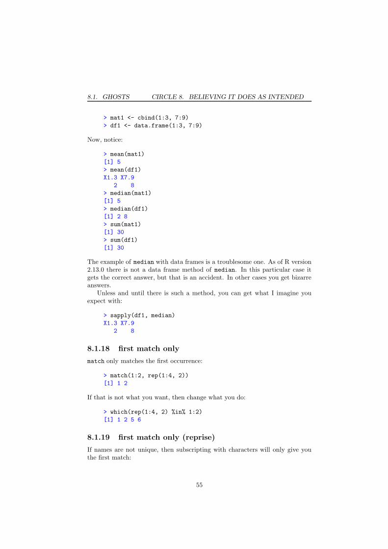
8.1. GHOSTS CIRCLE 8. BELIEVING IT DOES AS INTENDED
> mat1 <- cbind(1:3, 7:9)
> df1 <- data.frame(1:3, 7:9)
Now, notice:
> mean(mat1)
[1] 5
> mean(df1)
X1.3 X7.9
2 8
> median(mat1)
[1] 5
> median(df1)
[1] 2 8
> sum(mat1)
[1] 30
> sum(df1)
[1] 30
The example of median with data frames is a troublesome one. As of R version2.13.0 there is not a data frame method of median. In this particular case itgets the correct answer, but that is an accident. In other cases you get bizarreanswers.
Unless and until there is such a method, you can get what I imagine youexpect with:
> sapply(df1, median)
X1.3 X7.9
2 8
8.1.18 first match only
match only matches the first occurrence:
> match(1:2, rep(1:4, 2))
[1] 1 2
If that is not what you want, then change what you do:
> which(rep(1:4, 2) %in% 1:2)
[1] 1 2 5 6
8.1.19 first match only (reprise)
If names are not unique, then subscripting with characters will only give youthe first match:
55
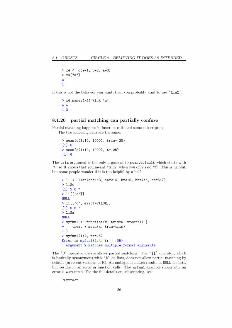
8.1. GHOSTS CIRCLE 8. BELIEVING IT DOES AS INTENDED
> x4 <- c(a=1, b=2, a=3)
> x4["a"]
a
1
If this is not the behavior you want, then you probably want to use 8 %in% 8 :
> x4[names(x4) %in% ’a’]
a a
1 3
8.1.20 partial matching can partially confuse
Partial matching happens in function calls and some subscripting.The two following calls are the same:
> mean(c(1:10, 1000), trim=.25)
[1] 6
> mean(c(1:10, 1000), t=.25)
[1] 6
The trim argument is the only argument to mean.default which starts with“t” so R knows that you meant “trim” when you only said “t”. This is helpful,but some people wonder if it is too helpful by a half.
> l1 <- list(aa=1:3, ab=2:4, b=3:5, bb=4:6, cc=5:7)
> l1$c
[1] 5 6 7
> l1[[’c’]]
NULL
> l1[[’c’, exact=FALSE]]
[1] 5 6 7
> l1$a
NULL
> myfun1 <- function(x, trim=0, treat=1) {+ treat * mean(x, trim=trim)
+ }> myfun1(1:4, tr=.5)
Error in myfun1(1:4, tr = .05) :
argument 2 matches multiple formal arguments
The 8 $ 8 operator always allows partial matching. The 8 [[ 8 operator, whichis basically synonymous with 8 $ 8 on lists, does not allow partial matching bydefault (in recent versions of R). An ambiguous match results in NULL for lists,but results in an error in function calls. The myfun1 example shows why anerror is warranted. For the full details on subscripting, see:
?Extract
56

8.1. GHOSTS CIRCLE 8. BELIEVING IT DOES AS INTENDED
Here are the rules for argument matching in function calls, but first some vocab-ulary: A formal argument is one of the argument names in the definition of thefunction. The mean.default function has 4 formal arguments (x, trim, na.rmand 8 ... 8 ). A tag is the string used in a call to indicate which formal argumentis meant. We used “t” as a tag in a call to mean (and hence to mean.default).There is a partial match if all the characters of the tag match the start of theformal argument.
• If a tag matches a formal argument exactly, then the two are bound.
• Unmatched tags are partially matched to unmatched formal arguments.
• An error occurs if any tag partially matches more than one formal argu-ment not already bound.
• (Positional matching) Unmatched formal arguments are bound to un-named (no tag) arguments in the call, based on the order in the calland of the formal arguments.
• If 8 ... 8 is among the formal arguments, any formal arguments after8 ... 8 are only matched exactly.
• If 8 ... 8 is among the formal arguments, any unmatched arguments inthe call, tagged or not, are taken up by the 8 ... 8 formal argument.
• An error occurs if any supplied arguments in the call are unmatched.
The place where partial matching is most likely to bite you is in calls that take afunction as an argument and you pass in additional arguments for the function.For example:
apply(xmat, 2, mean, trim=.2)
If the apply function had an argument that matched or partially matched“trim”, then apply would get the trim value, not mean.
There are two strategies in general use to reduce the possibility of suchcollisions:
• The apply family tends to have arguments that are in all capitals, andhence unlikely to collide with arguments of other functions that tend tobe in lower case.
• Optimization functions tend to put the 8 ... 8 (which is meant to be givento the function that is an argument) among the first of its arguments. Thusadditional arguments to the optimizer (as opposed to the function beingoptimized) need to be given by their full names.
Neither scheme is completely satisfactory—you can still get unexpected colli-sions in various ways. If you do (and you figure out what is happening), thenyou can include all of the arguments in question in your call.
57
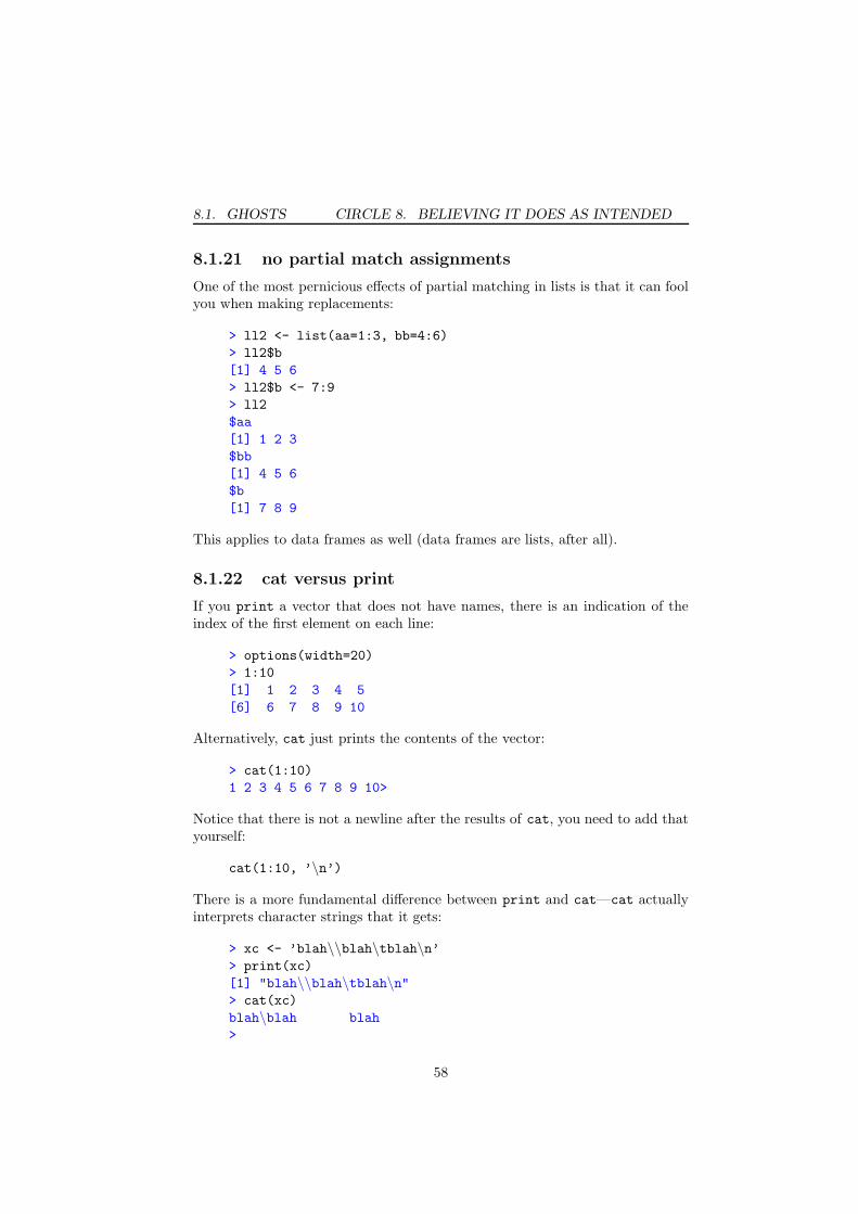
8.1. GHOSTS CIRCLE 8. BELIEVING IT DOES AS INTENDED
8.1.21 no partial match assignments
One of the most pernicious effects of partial matching in lists is that it can foolyou when making replacements:
> ll2 <- list(aa=1:3, bb=4:6)
> ll2$b
[1] 4 5 6
> ll2$b <- 7:9
> ll2
$aa
[1] 1 2 3
$bb
[1] 4 5 6
$b
[1] 7 8 9
This applies to data frames as well (data frames are lists, after all).
8.1.22 cat versus print
If you print a vector that does not have names, there is an indication of theindex of the first element on each line:
> options(width=20)
> 1:10
[1] 1 2 3 4 5
[6] 6 7 8 9 10
Alternatively, cat just prints the contents of the vector:
> cat(1:10)
1 2 3 4 5 6 7 8 9 10>
Notice that there is not a newline after the results of cat, you need to add thatyourself:
cat(1:10, ’\n’)
There is a more fundamental difference between print and cat—cat actuallyinterprets character strings that it gets:
> xc <- ’blah\\blah\tblah\n’> print(xc)
[1] "blah\\blah\tblah\n"> cat(xc)
blah\blah blah
>
58

8.1. GHOSTS CIRCLE 8. BELIEVING IT DOES AS INTENDED
Table 8.1: A few of the most important backslashed characters.
character meaning\\ backslash\n newline\t tab\" double quote (used when this is the string delimiter)\’ single quote (used when this is the string delimiter)
Strings are two-faced. One face is what the string actually says (this is whatcat gives you). The other face is a representation that allows you to see all ofthe characters—how the string is actually built—this is what print gives you.Do not confuse the two.
Reread this item—it is important. Important in the sense that if you don’tunderstand it, you are going to waste a few orders of magnitude more timefumbling around than it would take to understand.
8.1.23 backslashes
Backslashes are the escape character for R (and for Unix and C).Since backslash doesn’t mean backslash, there needs to be a way to mean
backslash. Quite logically that way is backslash-backslash:
> cat(’\\’)\>
Sometimes the text requires a backslash after the text has been interpreted. Inthe interpretation each pair of backslashes becomes one backslash. Backslashesgrow in powers of two.
There are two other very common characters involving backslash: \t meanstab and \n means newline. Table 8.1 shows the characters using backslash thatyou are most likely to encounter. You can see the entire list via:
?Quotes
Note that nchar (by default) gives the number of logical characters, not thenumber of keystrokes needed to create them:
> nchar(’\\’)[1] 1
8.1.24 internationalization
It may surprise some people, but not everyone writes with the same alphabet.To account for this R allows string encodings to include latin1 and UTF-8.
59

8.1. GHOSTS CIRCLE 8. BELIEVING IT DOES AS INTENDED
There is also the possibility of using different locales. The locale can affectthe order in which strings are sorted into.
The freedom of multiple string encodings and multiple locales gives you thechance to spend hours confusing yourself by mixing them.
For more information, do:
> ?Encoding
> ?locales
8.1.25 paths in Windows
Quite unfortunately Windows uses the backslash to separate directories in paths.Consider the R command:
attach(’C:\tmp\foo’)
This is confusing the two faces of strings. What that string actually contains is:C, colon, tab, m, p, formfeed, o, o. No backslashes at all. What should reallybe said is:
attach(’C:\\tmp\\foo’)
However, in all (or at least virtually all) cases R allows you to use slashes inplace of backslashes in Windows paths—it does the translation under the hood:
attach(’C:/tmp/foo’)
If you try to copy and paste a Windows path into R, you’ll get a string (which iswrong) along with some number of warnings about unrecognized escapes. Oneapproach is to paste into a command like:
scan(’’, ’’, n=1)
8.1.26 quotes
There are three types of quote marks, and a cottage industry has developed increating R functions that include the string “quote”. Table 8.2 lists functionsthat concern quoting in various ways. The bquote function is generally themost useful—it is similar to substitute.
Double-quotes and single-quotes—essentially synonymous—are used to de-limit character strings. If the quote that is delimiting the string is inside thestring, then it needs to be escaped with a backslash.
> ’"’
[1] "\""
A backquote (also called “backtick”) is used to delimit a name, often a namethat breaks the usual naming conventions of objects.
60
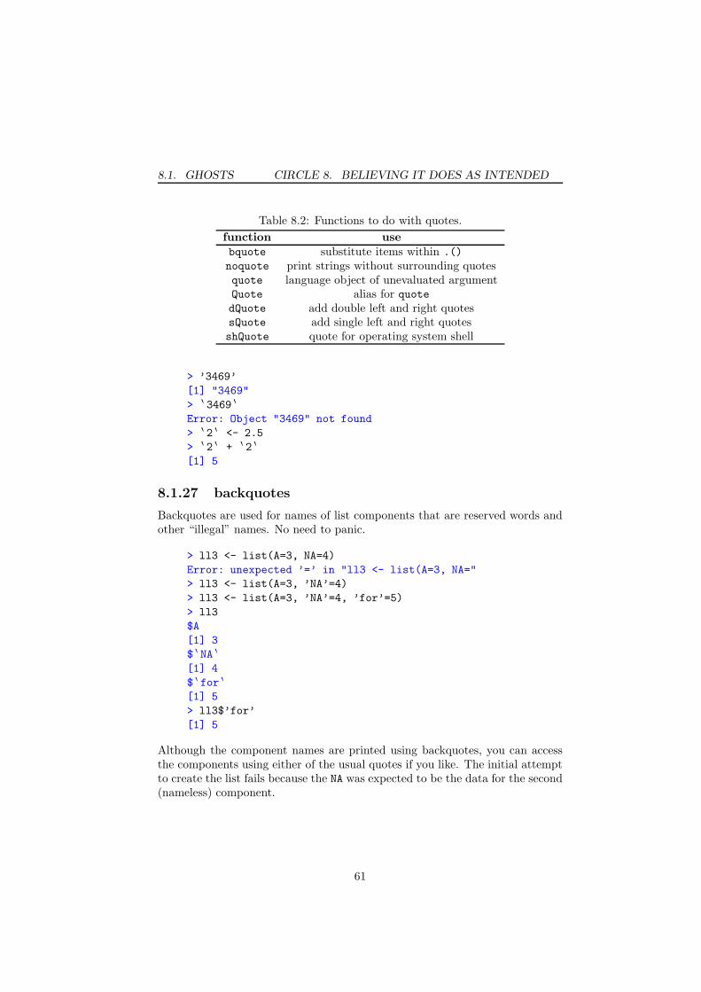
8.1. GHOSTS CIRCLE 8. BELIEVING IT DOES AS INTENDED
Table 8.2: Functions to do with quotes.
function usebquote substitute items within .()
noquote print strings without surrounding quotesquote language object of unevaluated argumentQuote alias for quotedQuote add double left and right quotessQuote add single left and right quotesshQuote quote for operating system shell
> ’3469’
[1] "3469"
> 8 3469 8
Error: Object "3469" not found
> 8 2 8 <- 2.5
> 8 2 8 + 8 2 8
[1] 5
8.1.27 backquotes
Backquotes are used for names of list components that are reserved words andother “illegal” names. No need to panic.
> ll3 <- list(A=3, NA=4)
Error: unexpected ’=’ in "ll3 <- list(A=3, NA="
> ll3 <- list(A=3, ’NA’=4)
> ll3 <- list(A=3, ’NA’=4, ’for’=5)
> ll3
$A
[1] 3
$ 8 NA 8
[1] 4
$ 8 for 8
[1] 5
> ll3$’for’
[1] 5
Although the component names are printed using backquotes, you can accessthe components using either of the usual quotes if you like. The initial attemptto create the list fails because the NA was expected to be the data for the second(nameless) component.
61

8.1. GHOSTS CIRCLE 8. BELIEVING IT DOES AS INTENDED
8.1.28 disappearing attributes
Most coercion functions strip the attributes from the object. For example, theresult of:
as.numeric(xmat)
will not be a matrix. A command that does the coercion but keeps the attributesis:
storage.mode(xmat) <- ’numeric’
8.1.29 disappearing attributes (reprise)
> x5 <- 1
> attr(x5, ’comment’) <- ’this is x5’
> attributes(x5)
$comment
[1] "this is x5"
> attributes(x5[1])
NULL
Subscripting almost always strips almost all attributes.If you want to keep attributes, then one solution is to create a class for your
object and write a method for that class for the 8 [ 8 function.
8.1.30 when space matters
Spaces, or their lack, seldom make a difference in R commands. Except thatspaces can make it much easier for humans to read (recall Uwe’s Maxim, page20).
There is an instance where space does matter to the R parser. Consider thestatement:
x<-3
This could be interpreted as either
x <- 3
or
x < -3
This should prompt you to use the spacebar on your keyboard. Most importantto make code legible to humans is to put spaces around the 8 <- 8 operator. Un-fortunately that does not solve the problem in this example—it is in comparisonsthat the space is absolutely required.
62
8.1. GHOSTS CIRCLE 8. BELIEVING IT DOES AS INTENDED
8.1.31 multiple comparisons
0 < x < 1
seems like a reasonable way to test if x is between 0 and 1. R doesn’t think so.The command that R agrees with is:
0 < x & x < 1
8.1.32 name masking
By default T and F are assigned to TRUE and FALSE, respectively. However, theycan be used as object names (but in S+ they can not be). This leads to twosuggestions:
1. It is extremely good practice to use TRUE and FALSE rather than T and F.
2. It is good practice to avoid using T and F as object names in order not tocollide with those that failed to follow suggestion 1.
It is also advisable to avoid using the names of common functions as objectnames. Two favorites are c and t.
And don’t call your matrix matrix, see:
fortune(’dog’)
Usually masking objects is merely confusing. However, if you mask a popularfunction name with your own function, it can verge on suicidal.
> c <- function(x) x * 100
> par(mfrow=c(2, 2))
Error in c(2, 2) : unused argument(s) (2)
If you get an extraordinarily strange error, it may be due to masking. Evasiveaction after the fact includes:
find(’c’)
if you know which function is the problem. To find the problem, you can try:
conflicts(detail=TRUE)
Another possibility for getting out of jail is to start R with --vanilla.
8.1.33 more sorting than sort
The order function is probably what you are looking for when sort doesn’t dothe sorting that you want. Uses of order include:
• sorting the rows of a matrix or data frame.
• sorting one vector based on values of another.
• breaking ties with additional variables.
63
8.1. GHOSTS CIRCLE 8. BELIEVING IT DOES AS INTENDED
8.1.34 sort.list not for lists
Do not be thinking that sort.list is to sort lists. You silly fool.In fact sorting doesn’t work on lists:
> sort(as.list(1:20))
Error in sort.int(x, na.last = na.last, ...) :
’x’ must be atomic
> sort.list(as.list(1:20))
Error in sort.list(as.list(1:20)) : ’x’ must be atomic
Have you called ’sort’ on a list?
If you have lists that you want sorted in some way, you’ll probably need to writeyour own function to do it.
8.1.35 search list shuffle
attach and load are very similar in purpose, but different in effect. attach
creates a new item in the search list while load puts its contents into the globalenvironment (the first place in the search list).
Often attach is the better approach to keep groups of objects separate.However, if you change directory into a location and want to have the existing.RData, then load is probably what you want.
Here is a scenario (that you don’t want):
• There exists a .RData in directory project1.
• You start R in some other directory and then change directory to project1.
• The global environment is from the initial directory.
• You attach .RData (from project1).
• You do some work, exit and save the workspace.
• You have just wiped out the original .RData in project1, losing the datathat was there.
8.1.36 source versus attach or load
Both attach and load put R objects onto the search list. The source functiondoes that as well, but when the starting point is code to create objects ratherthan actual objects.
There are conventions to try to keep straight which you should do. Filesof R code are often the extension “.R”. Other extensions for this include “.q”,“.rt”, “.Rscript”.
Extension for files of R objects include “.rda” and “.RData”.
64

8.1. GHOSTS CIRCLE 8. BELIEVING IT DOES AS INTENDED
8.1.37 string not the name
If you have a character string that contains the name of an object and you wantthe object, then use get:
funs <- c(’mean’, ’median’)
get(funs[2])(data)
If you found as.name and thought that would solve your problem, you wereright but you need one more step:
eval(as.name(funs[2]))(data)
8.1.38 get a component
The get function is extremely powerful, but it is not clairvoyant. If you say:
get(’myobj$comp’)
it thinks (quite rightly) you are asking for an object named ’myobj$comp’. Ifyou want the comp component of myobj, you have to say:
get(’myobj’)$comp
8.1.39 string not the name (encore)
If you have a character string that contains the name of a component that youwant to extract from a list, then you can not use the 8 $ 8 operator. You needto use 8 [[ 8 :
> mylist <- list(aaa=1:5, bbb=letters)
> subv <- ’aaa’
> mylist$subv
NULL
> # the next three lines are all the same
> mylist$aaa
[1] 1 2 3 4 5
> mylist[[’aaa’]]
[1] 1 2 3 4 5
> mylist[[subv]]
[1] 1 2 3 4 5
8.1.40 string not the name (yet again)
If you create a character string with paste and you want that to be the nameof an object, you can not use that on the left of an assignment:
> paste(’x’, 1, sep=’’) <- 3:5
Error: Target of assignment expands to non-language object
65
8.1. GHOSTS CIRCLE 8. BELIEVING IT DOES AS INTENDED
But assign will do this:
for(i in 1:n) assign(paste(’obj’, i, sep=’.’), mylist[[i]])
WARNING: An operation like this can land you in Circle 3 ([page 17] failing tovectorize—this example is anti-vectorizing) and/or the heresy of Circle 6 (page35).
As we have just seen with get, assigning to a name like ’myobj$comp’ isnot going to get you where you want to go—it will create an object with a non-standard name rather than modifying the comp component of myobj. Create acopy of the object, change the component in the copy, then assign the name tothe copy.
8.1.41 string not the name (still)
A formula can easily be created out of a character string:
> myvars <- paste(’V’, 1:9, sep=’’)
> myvars
[1] "V1" "V2" "V3" "V4" "V5" "V6" "V7" "V8" "V9"
> as.formula(paste(’y ~ ’, paste(myvars[c(3,5,8)],
+ collapse=’ + ’)))
y ~ V3 + V5 + V8
8.1.42 name not the argument
You may want to produce a plot or other output that states the dataset thatwas used. You might try something like:
myfun <- function(x, ...)
{plot(x, main=x, ...)
}
But that is going to produce a less than pleasing main title. The substitute
function along with deparse is probably what you are looking for.
myfun2 <- function(x, ...)
{plot(x, main=deparse(substitute(x)), ...)
}
66

8.1. GHOSTS CIRCLE 8. BELIEVING IT DOES AS INTENDED
8.1.43 unexpected else
Error: unexpected ’else’ in "else"
If you aren’t expecting ’else’ in ’else’, then where would you expect it?
While you may think that R is ludicrous for giving you such an error message,R thinks you are even more ludicrous for expecting what you did to work.
R takes input until it gets a complete statement, evaluates that statement,then takes more input. Here is how to get that error:
if(any(abs(x) > 1)) atan(x)
else asin(x)
When R gets to the end of the first line, it has a perfectly complete statementso it evaluates it. Now it finds a statement starting with ’else’—this makes nosense. Proper formatting is the key. If it is convenient, you can put the wholestatement on one line:
if(any(abs(x) > 1)) atan(x) else asin(x)
Alternatively, use curly braces (and a well-placed ’else’):
if(any(abs(x) > 1)) {atan(x)
} else {asin(x)
}
8.1.44 dropping dimensions
> xmat <- array(1:4, c(2,2))
> xmat[1,] # simple vector, not a matrix
[1] 1 3
> xmat[1, , drop=FALSE] # still a matrix
[,1] [,2]
[1,] 1 3
By default dimensions of arrays are dropped when subscripting makes the di-mension length 1. Subscripting with drop=FALSE overrides the default.
NOTE: Failing to use drop=FALSE inside functions is a major source of bugs.You only test the function when the subscript has length greater than 1. Thefunction fails once it hits a situation where the subscript is length 1—somewheredownstream a matrix is expected and there is a simple vector there instead.
NOTE: Failing to use drop=FALSE inside functions is a major source of bugs.
67
8.1. GHOSTS CIRCLE 8. BELIEVING IT DOES AS INTENDED
8.1.45 drop data frames
The drop function has no effect on a data frame. If you want dropping to bedone in a data frame, you need to use the drop argument in subscripting.
Dropping in data frames can be surprising (but it is logical).
> xdf <- data.frame(a=1:2, b=c(’v’, ’w’))
> xdf[1,] # data frame
a b
1 1 v
> drop(xdf[1,]) # data frame
a b
1 1 v
> xdf[1, , drop=TRUE] # list
$a
[1] 1
$b
[1] v
Levels: v w
> xdf[,1] # numeric vector
[1] 1 2
> xdf[, 1, drop=FALSE] # data frame
a
1 1
2 2
> drop(xdf[, 1, drop=FALSE]) # data frame
a
1 1
2 2
8.1.46 losing row names
The row names of a data frame are lost through dropping:
> xdf2 <- data.frame(a=1:4, b=42:45,
+ row.names=LETTERS[1:4])
> xdf2[, 1]
[1] 1 2 3 4
> as.matrix(xdf2)[, 1]
A B C D
1 2 3 4
Coercing to a matrix first will retain the row names, but possibly at the expenseof not getting the right values if the column types of the data frame are mixed.
> xdf2b <- data.frame(a=1:4, b=letters[21:24],
+ row.names=LETTERS[1:4])
68

8.1. GHOSTS CIRCLE 8. BELIEVING IT DOES AS INTENDED
> as.matrix(xdf2b)[,1]
A B C D
"1" "2" "3" "4"
> drop(as.matrix(xdf2b[, 1, drop=FALSE]))
A B C D
1 2 3 4
The final incantation, though a bit complicated, will give you the right thing.
8.1.47 apply function returning a vector
If you use apply with a function that returns a vector, that becomes the firstdimension of the result. This is likely not what you naively expect if you areoperating on rows:
> matrix(15:1, 3)
[,1] [,2] [,3] [,4] [,5]
[1,] 15 12 9 6 3
[2,] 14 11 8 5 2
[3,] 13 10 7 4 1
> apply(matrix(15:1, 3), 1, sort)
[,1] [,2] [,3]
[1,] 3 2 1
[2,] 6 5 4
[3,] 9 8 7
[4,] 12 11 10
[5,] 15 14 13
The naive expectation is really arrived at with:
t(apply(matrix(15:1, 3), 1, sort))
But note that no transpose is required if you operate on columns—the naiveexpectation holds in that case.
8.1.48 empty cells in tapply
If there are combinations of levels that do not appear, then tapply gives NA asthe answer (or NULL if simplify=FALSE):
> tapply(9, factor(1, levels=1:2), sum)
1 2
9 NA
> tapply(9, factor(1, levels=1:2), sum, simplify=FALSE)
$ 8 1 8
[1] 9
$ 8 2 8
NULL
69
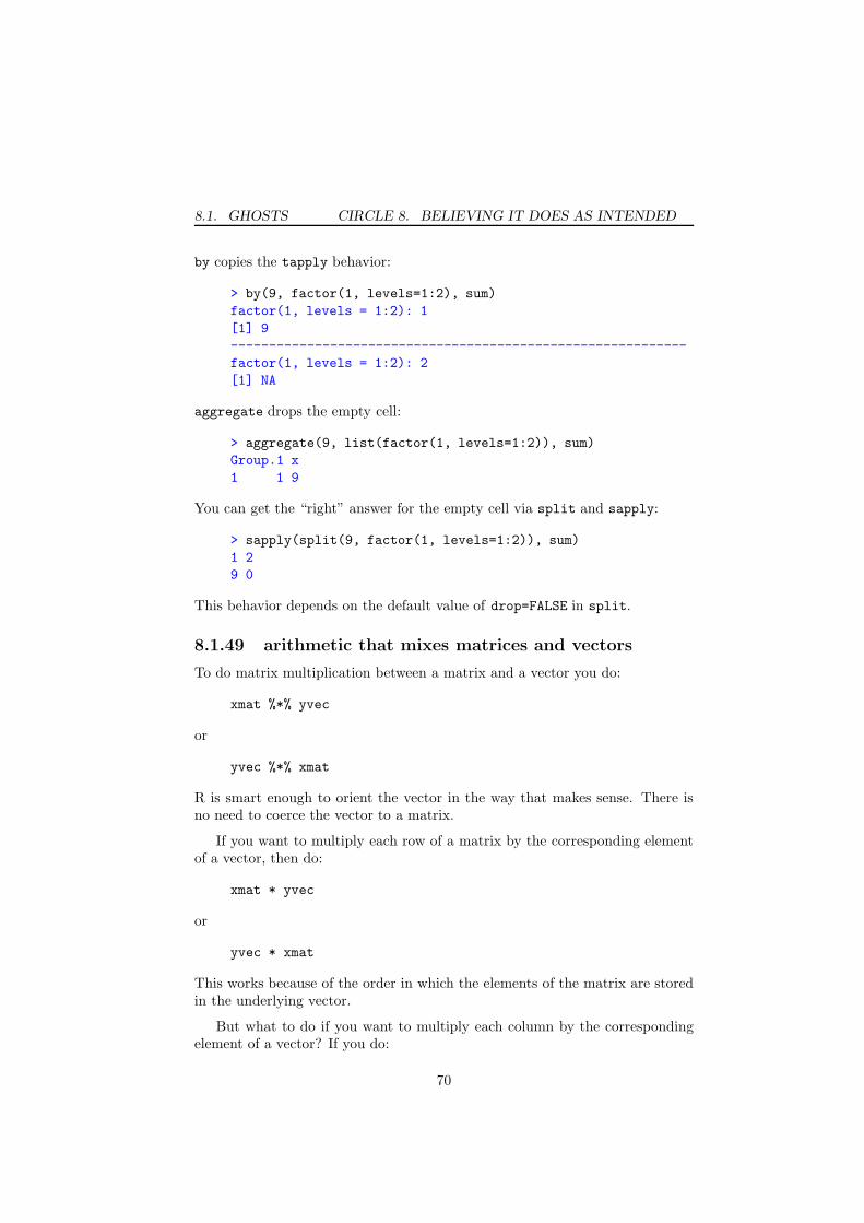
8.1. GHOSTS CIRCLE 8. BELIEVING IT DOES AS INTENDED
by copies the tapply behavior:
> by(9, factor(1, levels=1:2), sum)
factor(1, levels = 1:2): 1
[1] 9
------------------------------------------------------------
factor(1, levels = 1:2): 2
[1] NA
aggregate drops the empty cell:
> aggregate(9, list(factor(1, levels=1:2)), sum)
Group.1 x
1 1 9
You can get the “right” answer for the empty cell via split and sapply:
> sapply(split(9, factor(1, levels=1:2)), sum)
1 2
9 0
This behavior depends on the default value of drop=FALSE in split.
8.1.49 arithmetic that mixes matrices and vectors
To do matrix multiplication between a matrix and a vector you do:
xmat %*% yvec
or
yvec %*% xmat
R is smart enough to orient the vector in the way that makes sense. There isno need to coerce the vector to a matrix.
If you want to multiply each row of a matrix by the corresponding elementof a vector, then do:
xmat * yvec
or
yvec * xmat
This works because of the order in which the elements of the matrix are storedin the underlying vector.
But what to do if you want to multiply each column by the correspondingelement of a vector? If you do:
70

8.1. GHOSTS CIRCLE 8. BELIEVING IT DOES AS INTENDED
xmat * yvec
R does not check that the length of yvec matches the number of columns ofxmat and do the multiplication that you want. It does a multiplication that youdon’t want. There are a few ways to get your multiplication, among them are:
xmat * rep(yvec, each=nrow(xmat))
and
sweep(xmat, 2, yvec, ’*’)
The sweep function is quite general—make friends with it. The scale functioncan be useful for related problems.
8.1.50 single subscript of a data frame or array
Be careful of the number of commas when subscripting data frames and ma-trices. It is perfectly acceptable to subscript with no commas—this treats theobject as its underlying vector rather than a two dimensional object. In the caseof a data frame, the underlying object is a list and the single subscript refers tothe columns of the data frame. For matrices the underlying object is a vectorwith length equal to the number of rows times the number of columns.
8.1.51 non-numeric argument
> median(x)
Error in median.default(x) : need numeric data
If you get an error like this, it could well be because x is a factor.
8.1.52 round rounds to even
The round function rounds to even if it is rounding off an exact 5.Some people are surprised by this. I’m surprised that they are surprised—
rounding to even is the sensible thing to do. If you want a function that roundsup, write it yourself (possibly using the ceiling and floor functions, or byslightly increasing the size of the numbers).
Some times there is the surprise that an exact 5 is not rounded to even. Thiswill be due to Circle 1 (page 9)—what is apparently an exact 5 probably isn’t.
8.1.53 creating empty lists
You create a numeric vector of length 500 with:
numeric(500)
So obviously you create a list of length 500 with:
71
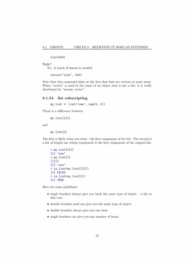
8.1. GHOSTS CIRCLE 8. BELIEVING IT DOES AS INTENDED
list(500)
Right?No. A touch of finesse is needed:
vector(’list’, 500)
Note that this command hints at the fact that lists are vectors in some sense.When “vector” is used in the sense of an object that is not a list, it is reallyshorthand for “atomic vector”.
8.1.54 list subscripting
my.list <- list(’one’, rep(2, 2))
There is a difference between
my.list[[1]]
and
my.list[1]
The first is likely what you want—the first component of the list. The second isa list of length one whose component is the first component of the original list.
> my.list[[1]]
[1] "one"
> my.list[1]
[[1]]
[1] "one"
> is.list(my.list[[1]])
[1] FALSE
> is.list(my.list[1])
[1] TRUE
Here are some guidelines:
• single brackets always give you back the same type of object – a list inthis case.
• double brackets need not give you the same type of object.
• double brackets always give you one item.
• single brackets can give you any number of items.
72

8.1. GHOSTS CIRCLE 8. BELIEVING IT DOES AS INTENDED
8.1.55 NULL or delete
If you have a list xl and you want component comp not to be there any more,you have some options. If comp is the index of the component in question, thenthe most transparent approach is:
xl <- xl[-comp]
In any case you can do:
xl[[comp]] <- NULL
or
xl[comp] <- NULL
The first two work in S+ as well, but the last one does not—it has no effect inS+.
If you want the component to stay there but to be NULL, then do:
xl[comp] <- list(NULL)
Notice single brackets, not double brackets.
8.1.56 disappearing components
A for loop can drop components of a list that it is modifying.
> xl.in <- list(A=c(a=3, z=4), B=NULL, C=c(w=8), D=NULL)
> xl.out <- vector(’list’, 4); names(xl.out) <- names(xl.in)
> for(i in 1:4) xl.out[[i]] <- names(xl.in[[i]])
> xl.out # not right
$A
[1] "a" "z"
$C
NULL
$D
[1] "w"
> xl.out2 <- lapply(xl.in, names)
> xl.out2
$A
[1] "a" "z"
$B
NULL
$C
[1] "w"
$D
NULL
73
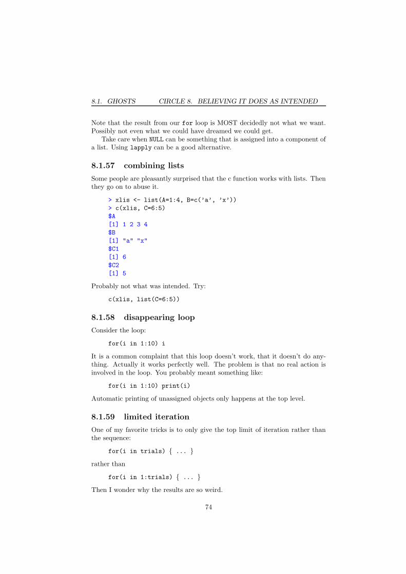
8.1. GHOSTS CIRCLE 8. BELIEVING IT DOES AS INTENDED
Note that the result from our for loop is MOST decidedly not what we want.Possibly not even what we could have dreamed we could get.
Take care when NULL can be something that is assigned into a component ofa list. Using lapply can be a good alternative.
8.1.57 combining lists
Some people are pleasantly surprised that the c function works with lists. Thenthey go on to abuse it.
> xlis <- list(A=1:4, B=c(’a’, ’x’))
> c(xlis, C=6:5)
$A
[1] 1 2 3 4
$B
[1] "a" "x"
$C1
[1] 6
$C2
[1] 5
Probably not what was intended. Try:
c(xlis, list(C=6:5))
8.1.58 disappearing loop
Consider the loop:
for(i in 1:10) i
It is a common complaint that this loop doesn’t work, that it doesn’t do any-thing. Actually it works perfectly well. The problem is that no real action isinvolved in the loop. You probably meant something like:
for(i in 1:10) print(i)
Automatic printing of unassigned objects only happens at the top level.
8.1.59 limited iteration
One of my favorite tricks is to only give the top limit of iteration rather thanthe sequence:
for(i in trials) { ... }rather than
for(i in 1:trials) { ... }Then I wonder why the results are so weird.
74

8.1. GHOSTS CIRCLE 8. BELIEVING IT DOES AS INTENDED
8.1.60 too much iteration
for(i in 1:length(x)) { ... }
is fine if x has a positive length. However, if its length is zero, then R wants todo two iterations. A safer idiom is:
for(i in seq along(x)) { ... }
or if you want to be compatible with S+:
for(i in seq(along=x)) { ... }
8.1.61 wrong iterate
The for iterate can be from any vector. This makes looping much more generalthan in most other languages, but can allow some users to become confused:
nums <- seq(-1, 1, by=.01)
ans <- NULL
for(i in nums) ans[i] <- i^2
This has two things wrong with it. You should recognize that we have tried(but failed) to visit Circle 2 (page 12) here, and the index on ans is not whatthe user is expecting. Better would be:
nums <- seq(-1, 1, by=.01)
ans <- numeric(length(nums))
for(i in seq(along=nums)) ans[i] <- nums[i]^2
Even better, of course, would be to avoid a loop altogether. That is possible inthis case, perhaps not in a real application.
8.1.62 wrong iterate (encore)
A loop like:
for(i in 0:9) {this.x <- x[i]
...
does not do as intended. While C and some other languages index from 0, Rindexes from 1. The unfortunate thing in this case is that an index of 0 isallowed in R, it just doesn’t do what is wanted.
75
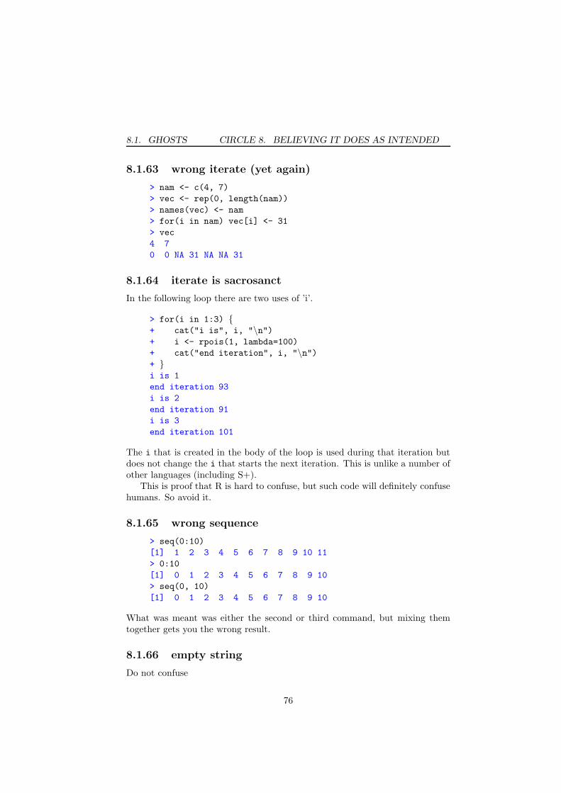
8.1. GHOSTS CIRCLE 8. BELIEVING IT DOES AS INTENDED
8.1.63 wrong iterate (yet again)
> nam <- c(4, 7)
> vec <- rep(0, length(nam))
> names(vec) <- nam
> for(i in nam) vec[i] <- 31
> vec
4 7
0 0 NA 31 NA NA 31
8.1.64 iterate is sacrosanct
In the following loop there are two uses of ’i’.
> for(i in 1:3) {+ cat("i is", i, "\n")+ i <- rpois(1, lambda=100)
+ cat("end iteration", i, "\n")+ }i is 1
end iteration 93
i is 2
end iteration 91
i is 3
end iteration 101
The i that is created in the body of the loop is used during that iteration butdoes not change the i that starts the next iteration. This is unlike a number ofother languages (including S+).
This is proof that R is hard to confuse, but such code will definitely confusehumans. So avoid it.
8.1.65 wrong sequence
> seq(0:10)
[1] 1 2 3 4 5 6 7 8 9 10 11
> 0:10
[1] 0 1 2 3 4 5 6 7 8 9 10
> seq(0, 10)
[1] 0 1 2 3 4 5 6 7 8 9 10
What was meant was either the second or third command, but mixing themtogether gets you the wrong result.
8.1.66 empty string
Do not confuse
76

8.1. GHOSTS CIRCLE 8. BELIEVING IT DOES AS INTENDED
character(0)
with
""
The first is a vector of length zero whose elements would be character if it hadany. The second is a vector of length one, and the element that it has is theempty string.
The result of nchar on the first object is a numeric vector of length zero,while the result of nchar on the second object is 0—that is, a vector of lengthone whose first and only element is zero.
> nchar(character(0))
numeric(0)
> nchar("")
[1] 0
8.1.67 NA the string
There is a missing value for character data. In normal printing (with quotesaround strings) the missing value is printed as NA; but when quotes are notused, it is printed as <NA>. This is to distinguish it from the string ’NA’:
> cna <- c(’missing value’=NA, ’real string’=’NA’)
> cna
missing value real string
NA "NA"
> noquote(cna)
missing value real string
<NA> NA
NA the string really does happen. It is Nabisco in finance, North Americain geography, and possibly sodium in chemistry. There are circumstances—particularly when reading data into R—where NA the string becomes NA themissing value. Having a name or dimname that is accidentally a missing valuecan be an unpleasant experience.
If you have missing values in a character vector, you may want to take someevasive action when operating on the vector:
> people <- c(’Alice’, NA, ’Eve’)
> paste(’hello’, people)
[1] "hello Alice" "hello NA" "hello Eve"
> ifelse(is.na(people), people, paste(’hello’, people))
[1] "hello Alice" NA "hello Eve"
77

8.1. GHOSTS CIRCLE 8. BELIEVING IT DOES AS INTENDED
8.1.68 capitalization
Some people have a hard time with the fact that R is case-sensitive. Being case-sensitive is a good thing. The case of letters REALLy doEs MakE a diFFerencE.
8.1.69 scoping
Scoping problems are uncommon in R because R uses scoping rules that areintuitive in almost all cases. An issue with scoping is most likely to arise whenmoving S+ code into R.
Perhaps you want to know what “scoping” means. In the evaluator if atsome point an object of a certain name, z say, is needed, then we need to knowwhere to look for z. Scoping is the set of rules of where to look.
Here is a small example:
> z <- ’global’
> myTopFun
function () {subfun <- function() {
paste(’used:’, z)
}z <- ’inside myTopFun’
subfun()
}> myTopFun()
[1] "used: inside myTopFun"
The z that is used is the one inside the function. Let’s think a bit about what isnot happening. At the point in time that subfun is defined, the only z about isthe one in the global environment. When the object is assigned is not important.Where the object is assigned is important. Also important is the state of therelevant environments when the function is evaluated.
8.1.70 scoping (encore)
The most likely place to find a scoping problem is with the modeling functions.Let’s explore with some examples.
> scope1
function () {sub1 <- function(form) coef(lm(form))
xx <- rnorm(12)
yy <- rnorm(12, xx)
form1 <- yy ~ xx
sub1(form1)
}> scope1()
78
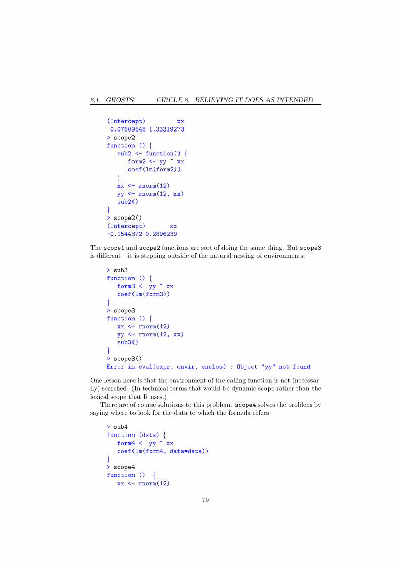
8.1. GHOSTS CIRCLE 8. BELIEVING IT DOES AS INTENDED
(Intercept) xx
-0.07609548 1.33319273
> scope2
function () {sub2 <- function() {
form2 <- yy ~ xx
coef(lm(form2))
}xx <- rnorm(12)
yy <- rnorm(12, xx)
sub2()
}> scope2()
(Intercept) xx
-0.1544372 0.2896239
The scope1 and scope2 functions are sort of doing the same thing. But scope3is different—it is stepping outside of the natural nesting of environments.
> sub3
function () {form3 <- yy ~ xx
coef(lm(form3))
}> scope3
function () {xx <- rnorm(12)
yy <- rnorm(12, xx)
sub3()
}> scope3()
Error in eval(expr, envir, enclos) : Object "yy" not found
One lesson here is that the environment of the calling function is not (necessar-ily) searched. (In technical terms that would be dynamic scope rather than thelexical scope that R uses.)
There are of course solutions to this problem. scope4 solves the problem bysaying where to look for the data to which the formula refers.
> sub4
function (data) {form4 <- yy ~ xx
coef(lm(form4, data=data))
}> scope4
function () {xx <- rnorm(12)
79
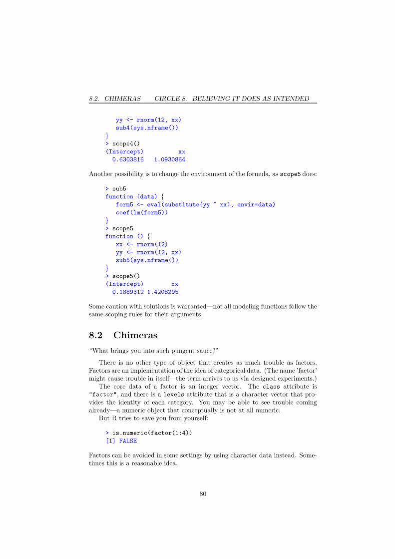
8.2. CHIMERAS CIRCLE 8. BELIEVING IT DOES AS INTENDED
yy <- rnorm(12, xx)
sub4(sys.nframe())
}> scope4()
(Intercept) xx
0.6303816 1.0930864
Another possibility is to change the environment of the formula, as scope5 does:
> sub5
function (data) {form5 <- eval(substitute(yy ~ xx), envir=data)
coef(lm(form5))
}> scope5
function () {xx <- rnorm(12)
yy <- rnorm(12, xx)
sub5(sys.nframe())
}> scope5()
(Intercept) xx
0.1889312 1.4208295
Some caution with solutions is warranted—not all modeling functions follow thesame scoping rules for their arguments.
8.2 Chimeras
“What brings you into such pungent sauce?”
There is no other type of object that creates as much trouble as factors.Factors are an implementation of the idea of categorical data. (The name ’factor’might cause trouble in itself—the term arrives to us via designed experiments.)
The core data of a factor is an integer vector. The class attribute is"factor", and there is a levels attribute that is a character vector that pro-vides the identity of each category. You may be able to see trouble comingalready—a numeric object that conceptually is not at all numeric.
But R tries to save you from yourself:
> is.numeric(factor(1:4))
[1] FALSE
Factors can be avoided in some settings by using character data instead. Some-times this is a reasonable idea.
80

8.2. CHIMERAS CIRCLE 8. BELIEVING IT DOES AS INTENDED
Figure 8.2: The treacherous to kin and the treacherous to country by SandroBotticelli.
81

8.2. CHIMERAS CIRCLE 8. BELIEVING IT DOES AS INTENDED
8.2.1 numeric to factor to numeric
While in general factors do not refer to numbers, they may do. In which casewe have even more room for confusion.
> as.numeric(factor(101:103))
[1] 1 2 3
If you were expecting:
[1] 101 102 103
shame on you.If your factor represents numbers and you want to recover those numbers
from the factor, then you need a more circuitous route to get there:
as.numeric(as.character(factor(101:103)))
Slightly more efficient, but harder to remember is:
as.numeric(levels(f))[f]
where f is the factor.
8.2.2 cat factor
Using cat on any factor will just give the core data:
> cat(factor(letters[1:5]))
1 2 3 4 5>
8.2.3 numeric to factor accidentally
When using read.table or its friends, it is all too common for a column of datathat is meant to be numeric to be read as a factor. This happens if na.stringsis not properly set, if there is a bogus entry in the column, and probably manyother circumstances.
This is dynamite.
The data are thought to be numeric. They are in fact numeric (at least sortof), but decidedly not with the numbers that are intended. Hence you can endup with data that ’works’ but produces complete garbage.
When processing the data, the construct:
as.numeric(as.character(x))
guards you against this occurring. If x is already the correct numbers, thennothing happens except wasting a few microseconds. If x is accidentally afactor, then it becomes the correct numbers (at least mostly—depending onwhy it became a factor there may be some erroneously missing values).
82
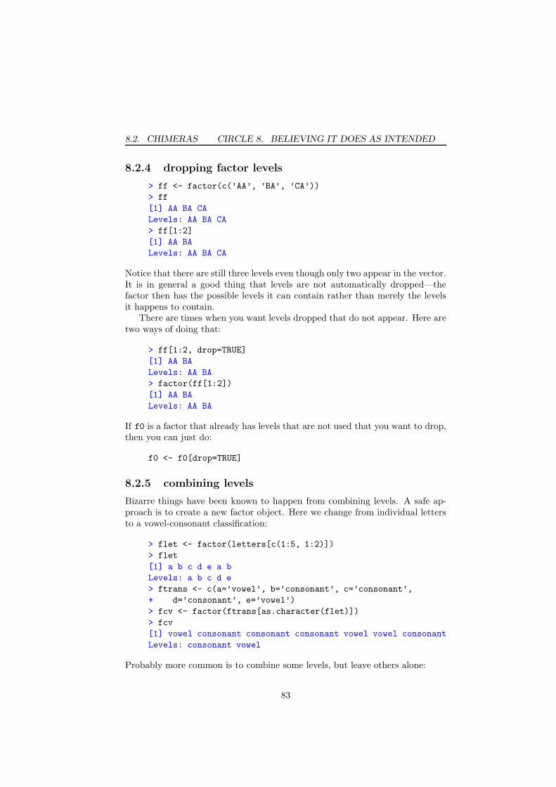
8.2. CHIMERAS CIRCLE 8. BELIEVING IT DOES AS INTENDED
8.2.4 dropping factor levels
> ff <- factor(c(’AA’, ’BA’, ’CA’))
> ff
[1] AA BA CA
Levels: AA BA CA
> ff[1:2]
[1] AA BA
Levels: AA BA CA
Notice that there are still three levels even though only two appear in the vector.It is in general a good thing that levels are not automatically dropped—thefactor then has the possible levels it can contain rather than merely the levelsit happens to contain.
There are times when you want levels dropped that do not appear. Here aretwo ways of doing that:
> ff[1:2, drop=TRUE]
[1] AA BA
Levels: AA BA
> factor(ff[1:2])
[1] AA BA
Levels: AA BA
If f0 is a factor that already has levels that are not used that you want to drop,then you can just do:
f0 <- f0[drop=TRUE]
8.2.5 combining levels
Bizarre things have been known to happen from combining levels. A safe ap-proach is to create a new factor object. Here we change from individual lettersto a vowel-consonant classification:
> flet <- factor(letters[c(1:5, 1:2)])
> flet
[1] a b c d e a b
Levels: a b c d e
> ftrans <- c(a=’vowel’, b=’consonant’, c=’consonant’,
+ d=’consonant’, e=’vowel’)
> fcv <- factor(ftrans[as.character(flet)])
> fcv
[1] vowel consonant consonant consonant vowel vowel consonant
Levels: consonant vowel
Probably more common is to combine some levels, but leave others alone:
83
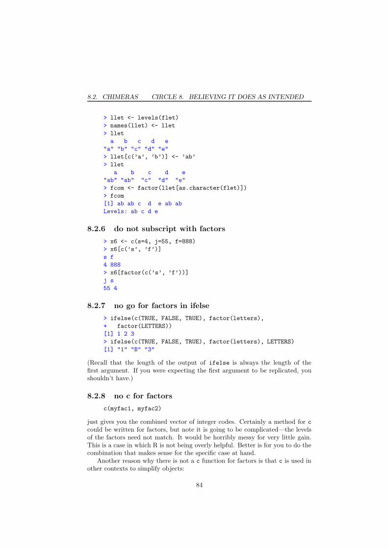
8.2. CHIMERAS CIRCLE 8. BELIEVING IT DOES AS INTENDED
> llet <- levels(flet)
> names(llet) <- llet
> llet
a b c d e
"a" "b" "c" "d" "e"
> llet[c(’a’, ’b’)] <- ’ab’
> llet
a b c d e
"ab" "ab" "c" "d" "e"
> fcom <- factor(llet[as.character(flet)])
> fcom
[1] ab ab c d e ab ab
Levels: ab c d e
8.2.6 do not subscript with factors
> x6 <- c(s=4, j=55, f=888)
> x6[c(’s’, ’f’)]
s f
4 888
> x6[factor(c(’s’, ’f’))]
j s
55 4
8.2.7 no go for factors in ifelse
> ifelse(c(TRUE, FALSE, TRUE), factor(letters),
+ factor(LETTERS))
[1] 1 2 3
> ifelse(c(TRUE, FALSE, TRUE), factor(letters), LETTERS)
[1] "1" "B" "3"
(Recall that the length of the output of ifelse is always the length of thefirst argument. If you were expecting the first argument to be replicated, youshouldn’t have.)
8.2.8 no c for factors
c(myfac1, myfac2)
just gives you the combined vector of integer codes. Certainly a method for c
could be written for factors, but note it is going to be complicated—the levelsof the factors need not match. It would be horribly messy for very little gain.This is a case in which R is not being overly helpful. Better is for you to do thecombination that makes sense for the specific case at hand.
Another reason why there is not a c function for factors is that c is used inother contexts to simplify objects:
84
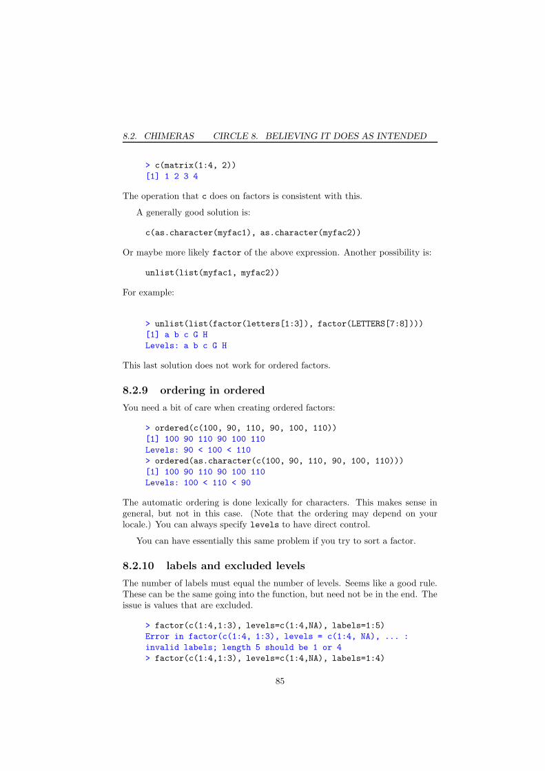
8.2. CHIMERAS CIRCLE 8. BELIEVING IT DOES AS INTENDED
> c(matrix(1:4, 2))
[1] 1 2 3 4
The operation that c does on factors is consistent with this.
A generally good solution is:
c(as.character(myfac1), as.character(myfac2))
Or maybe more likely factor of the above expression. Another possibility is:
unlist(list(myfac1, myfac2))
For example:
> unlist(list(factor(letters[1:3]), factor(LETTERS[7:8])))
[1] a b c G H
Levels: a b c G H
This last solution does not work for ordered factors.
8.2.9 ordering in ordered
You need a bit of care when creating ordered factors:
> ordered(c(100, 90, 110, 90, 100, 110))
[1] 100 90 110 90 100 110
Levels: 90 < 100 < 110
> ordered(as.character(c(100, 90, 110, 90, 100, 110)))
[1] 100 90 110 90 100 110
Levels: 100 < 110 < 90
The automatic ordering is done lexically for characters. This makes sense ingeneral, but not in this case. (Note that the ordering may depend on yourlocale.) You can always specify levels to have direct control.
You can have essentially this same problem if you try to sort a factor.
8.2.10 labels and excluded levels
The number of labels must equal the number of levels. Seems like a good rule.These can be the same going into the function, but need not be in the end. Theissue is values that are excluded.
> factor(c(1:4,1:3), levels=c(1:4,NA), labels=1:5)
Error in factor(c(1:4, 1:3), levels = c(1:4, NA), ... :
invalid labels; length 5 should be 1 or 4
> factor(c(1:4,1:3), levels=c(1:4,NA), labels=1:4)
85
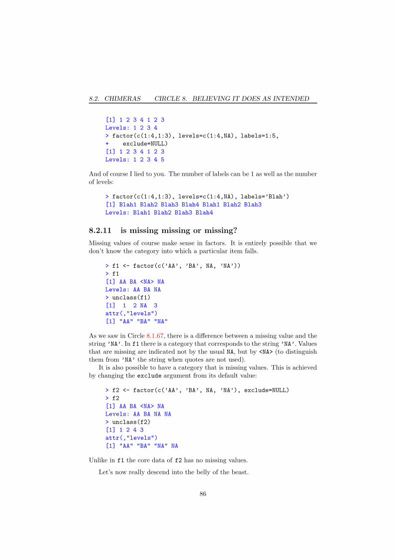
8.2. CHIMERAS CIRCLE 8. BELIEVING IT DOES AS INTENDED
[1] 1 2 3 4 1 2 3
Levels: 1 2 3 4
> factor(c(1:4,1:3), levels=c(1:4,NA), labels=1:5,
+ exclude=NULL)
[1] 1 2 3 4 1 2 3
Levels: 1 2 3 4 5
And of course I lied to you. The number of labels can be 1 as well as the numberof levels:
> factor(c(1:4,1:3), levels=c(1:4,NA), labels=’Blah’)
[1] Blah1 Blah2 Blah3 Blah4 Blah1 Blah2 Blah3
Levels: Blah1 Blah2 Blah3 Blah4
8.2.11 is missing missing or missing?
Missing values of course make sense in factors. It is entirely possible that wedon’t know the category into which a particular item falls.
> f1 <- factor(c(’AA’, ’BA’, NA, ’NA’))
> f1
[1] AA BA <NA> NA
Levels: AA BA NA
> unclass(f1)
[1] 1 2 NA 3
attr(,"levels")
[1] "AA" "BA" "NA"
As we saw in Circle 8.1.67, there is a difference between a missing value and thestring ’NA’. In f1 there is a category that corresponds to the string ’NA’. Valuesthat are missing are indicated not by the usual NA, but by <NA> (to distinguishthem from ’NA’ the string when quotes are not used).
It is also possible to have a category that is missing values. This is achievedby changing the exclude argument from its default value:
> f2 <- factor(c(’AA’, ’BA’, NA, ’NA’), exclude=NULL)
> f2
[1] AA BA <NA> NA
Levels: AA BA NA NA
> unclass(f2)
[1] 1 2 4 3
attr(,"levels")
[1] "AA" "BA" "NA" NA
Unlike in f1 the core data of f2 has no missing values.
Let’s now really descend into the belly of the beast.
86

8.2. CHIMERAS CIRCLE 8. BELIEVING IT DOES AS INTENDED
> f3 <- f2
> is.na(f3)[1] <- TRUE
> f3
[1] <NA> BA <NA> NA
Levels: AA BA NA NA
> unclass(f3)
[1] NA 2 4 3
attr(,"levels")
[1] "AA" "BA" "NA" NA
Here we have a level that is missing values, we also have a missing value in thecore data.1
To summarize, there are two ways that missing values can enter a factor:
• Missing means we don’t know what category the item falls into.
• Missing is the category of items that (originally) had missing values.
8.2.12 data frame to character
> xdf3 <- data.frame(a=3:2, b=c(’x’, ’y’))
> as.character(xdf3[1,])
[1] "3" "1"
This is a hidden version of coercing a factor to character. One approach to getthe correct behavior is to use as.matrix:
> as.character(as.matrix(xdf3[1,]))
[1] "3" "x"
I’m not sure if it is less upsetting or more upsetting if you try coercing morethan one row of a data frame to character:
> as.character(xdf3)
[1] "c(3, 2)" "c(1, 2)"
If the columns of the data frame include factors or characters, then convertingto a matrix will automatically get you a characters:
> as.matrix(xdf3)
a b
[1,] "3" "x"
[2,] "2" "y"
1The author would be intrigued to hear of an application where this makes sense—an itemfor which it is unknown if it is missing or not.
87
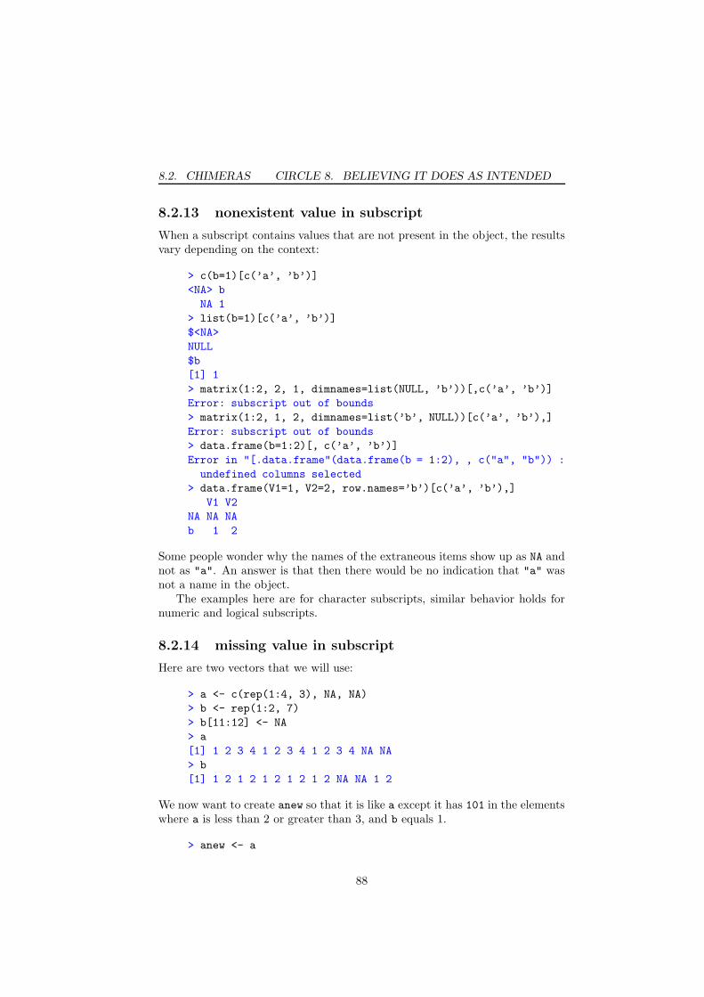
8.2. CHIMERAS CIRCLE 8. BELIEVING IT DOES AS INTENDED
8.2.13 nonexistent value in subscript
When a subscript contains values that are not present in the object, the resultsvary depending on the context:
> c(b=1)[c(’a’, ’b’)]
<NA> b
NA 1
> list(b=1)[c(’a’, ’b’)]
$<NA>
NULL
$b
[1] 1
> matrix(1:2, 2, 1, dimnames=list(NULL, ’b’))[,c(’a’, ’b’)]
Error: subscript out of bounds
> matrix(1:2, 1, 2, dimnames=list(’b’, NULL))[c(’a’, ’b’),]
Error: subscript out of bounds
> data.frame(b=1:2)[, c(’a’, ’b’)]
Error in "[.data.frame"(data.frame(b = 1:2), , c("a", "b")) :
undefined columns selected
> data.frame(V1=1, V2=2, row.names=’b’)[c(’a’, ’b’),]
V1 V2
NA NA NA
b 1 2
Some people wonder why the names of the extraneous items show up as NA andnot as "a". An answer is that then there would be no indication that "a" wasnot a name in the object.
The examples here are for character subscripts, similar behavior holds fornumeric and logical subscripts.
8.2.14 missing value in subscript
Here are two vectors that we will use:
> a <- c(rep(1:4, 3), NA, NA)
> b <- rep(1:2, 7)
> b[11:12] <- NA
> a
[1] 1 2 3 4 1 2 3 4 1 2 3 4 NA NA
> b
[1] 1 2 1 2 1 2 1 2 1 2 NA NA 1 2
We now want to create anew so that it is like a except it has 101 in the elementswhere a is less than 2 or greater than 3, and b equals 1.
> anew <- a
88

8.2. CHIMERAS CIRCLE 8. BELIEVING IT DOES AS INTENDED
> anew[(a < 2 | a > 3) & b == 1] <- 101
> anew
[1] 101 2 3 4 101 2 3 4 101 2 3 4 NA NA
There were three values changed in anew; let’s try again but give different valuesto those three:
> anew2 <- a
> anew2[(a < 2 | a > 3) & b == 1] <- 101:103
Error: NAs are not allowed in subscripted assignments
Now we get an error. Since the value being assigned into the vector has lengthgreater than 1, the assignment with missing values in the subscripts is ambigu-ous. R wisely refuses to do it (frustrating as it may be). There is a simplesolution, however:
> anew2[which((a < 2 | a > 3) & b == 1)] <- 101:103
> anew2
[1] 101 2 3 4 102 2 3 4 103 2 3 4 NA NA
The which function effectively treats NA as FALSE.
But we still have a problem in both anew and anew2. The 12th element ofa is 4 (and hence greater than 3) while the 12th element of b is NA. So we don’tknow if the 12th element of anew should be changed or not. The 12th elementof anew should be NA:
> anew[is.na(b) & (a < 2 | a > 3)] <- NA
> anew
[1] 101 2 3 4 101 2 3 4 101 2 3 NA NA NA
8.2.15 all missing subscripts
> letters[c(2,3)]
[1] "b" "c"
> letters[c(2,NA)]
[1] "b" NA
> letters[c(NA,NA)]
[1] NA NA NA NA NA NA NA NA NA NA NA NA
[13] NA NA NA NA NA NA NA NA NA NA NA NA
[25] NA NA
What is happening here is that by default NA is logical—that is the most specificmode (see Circle 8.1.8) so the last command is subscripting with logical valuesinstead of numbers. Logical subscripts are automatically replicated to be thelength of the object.
89

8.2. CHIMERAS CIRCLE 8. BELIEVING IT DOES AS INTENDED
8.2.16 missing value in if
if(NA) { # creates error
It is a rather common error for an if condition to be NA. When this occurs, itis common for the problem to be non-obvious. Debugging is called for in thatcase.
8.2.17 and and andand
An alternative title here could have been ’or or oror’.There are two ’and’ operators and two ’or’ operators:– 8 && 8 and 8 || 8 go with if
– 8 & 8 and 8 | 8 go with ifelse8 && 8 and 8 || 8 , like if, expect single element inputs. Because they only dealwith single elements, they can do shortcuts. If the answer is known with thefirst (left) argument, then there is no need to evaluate the second.
> if(TRUE || stop()) 4 else 5
[1] 4
> if(TRUE && stop()) 4 else 5
Error:
> if(FALSE || stop()) 4 else 5
Error:
> if(FALSE && stop()) 4 else 5
[1] 5
This can be used to make sure that it is safe to perform a test, as in:
> if(ncol(x) > 6) { ...
Error in if (ncol(x) > 6) : argument is of length zero
> if(is.matrix(x) && ncol(x) > 6) { ... # okay
Note that in the last line x is excluded from being a data frame. If you want toallow both data frames and matrices, then testing the length of dim(x) wouldbe an approach.
8.2.18 equal and equalequal
Just because 8 && 8 and 8 & 8 have similar purposes, don’t go thinking that 8 == 8
and 8 = 8 are similar. Completely different.Fortunately R keeps you from making this error in a key context:
> if(x = 7) { ...
Error: unexpected ’=’ in "if(x ="
> if(x == 7) { ... # okay
The difference is:– 8 == 8 is a logical operator that tests equality.– 8 = 8 is an assignment operator similar to 8<- 8 (but see Circle 8.2.26).
90

8.2. CHIMERAS CIRCLE 8. BELIEVING IT DOES AS INTENDED
8.2.19 is.integer
is.integer is a test of how the data are stored, it does not test if the numbersare logically integers:
> is.integer(c(4, 0, 3))
[1] FALSE
The key thing to say here is that, almost surely, you do not care if an object isstored as integer. It is important if you are sending the data to C or Fortran.Otherwise you can bask in the ease of letting R take care of details so you canthink about the big picture.
If you really want integers (that is, stored in integer format), then use “L”:
> is.integer(c(4L, 0L, 3L))
[1] TRUE
> is.integer(c(4L, 0L, 3))
[1] FALSE
The 8 : 8 operator is one of the few places in R where integers are produced :
> is.integer(1:3)
[1] TRUE
> is.integer(c(1:3, 4))
[1] FALSE
> is.integer(c(1:3, 4:4))
[1] TRUE
Given experience with other languages, you may expect:
> is.integer( 4. )
[1] FALSE
> is.integer( 4 )
[1] FALSE
the first comand above to be FALSE and the second to be TRUE. That is, thatusing a decimal point signifies that you want a floating point number as opposedto an integer. As you see R has a fondness for floating point numbers.
You can coerce to integer, but (as always) be careful what you ask for:
> as.integer(c(0, 1, -2.99, 2.99))
[1] 0 1 -2 2
8.2.20 is.numeric, as.numeric with integers
An integer vector tests TRUE with is.numeric. However, as.numeric changesit from storage mode integer to storage mode double. If you care about it beinginteger, then you want to use as.integer.
91
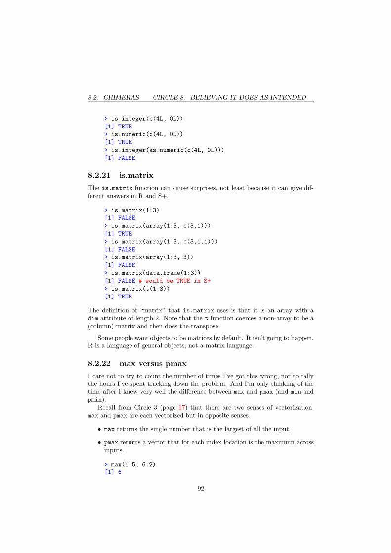
8.2. CHIMERAS CIRCLE 8. BELIEVING IT DOES AS INTENDED
> is.integer(c(4L, 0L))
[1] TRUE
> is.numeric(c(4L, 0L))
[1] TRUE
> is.integer(as.numeric(c(4L, 0L)))
[1] FALSE
8.2.21 is.matrix
The is.matrix function can cause surprises, not least because it can give dif-ferent answers in R and S+.
> is.matrix(1:3)
[1] FALSE
> is.matrix(array(1:3, c(3,1)))
[1] TRUE
> is.matrix(array(1:3, c(3,1,1)))
[1] FALSE
> is.matrix(array(1:3, 3))
[1] FALSE
> is.matrix(data.frame(1:3))
[1] FALSE # would be TRUE in S+
> is.matrix(t(1:3))
[1] TRUE
The definition of “matrix” that is.matrix uses is that it is an array with adim attribute of length 2. Note that the t function coerces a non-array to be a(column) matrix and then does the transpose.
Some people want objects to be matrices by default. It isn’t going to happen.R is a language of general objects, not a matrix language.
8.2.22 max versus pmax
I care not to try to count the number of times I’ve got this wrong, nor to tallythe hours I’ve spent tracking down the problem. And I’m only thinking of thetime after I knew very well the difference between max and pmax (and min andpmin).
Recall from Circle 3 (page 17) that there are two senses of vectorization.max and pmax are each vectorized but in opposite senses.
• max returns the single number that is the largest of all the input.
• pmax returns a vector that for each index location is the maximum acrossinputs.
> max(1:5, 6:2)
[1] 6
92

8.2. CHIMERAS CIRCLE 8. BELIEVING IT DOES AS INTENDED
> pmax(1:5, 6:2)
[1] 6 5 4 4 5
The ’p’ in pmax stands for ’parallel’.
8.2.23 all.equal returns a surprising value
We met all.equal in Circle 1 (page 9) as an alternative to 8 == 8 . Numericalerror causes 8 == 8 not to provide a useful result in many cases.
if(all(x == y)) { # wrong if there is numerical error
if(all.equal(x, y)) { # WRONG, not FALSE when not equal
if(isTRUE(all.equal(x, y)) { # right
8.2.24 all.equal is not identical
The purpose of all.equal is to compare items that may have some fuzzinessto them. Sometimes the fuzziness that all.equal sees can be surprising:
> all.equal(as.numeric(NA), 0/0)
[1] TRUE
The identical function allows for no fuzziness at all:
> identical(as.numeric(NA), 0/0)
[1] FALSE
8.2.25 identical really really means identical
> xi <- 1:10
> yi <- 1:10
> identical(xi, yi[1:10])
[1] TRUE
> yi[11] <- 11
> identical(xi, yi[1:10])
[1] FALSE
> zi <- 1:10
> zi[11] <- 11L
> identical(xi, zi[1:10])
[1] TRUE
xi is stored as type integer. But once yi has been given one double value, it isstored as double.
As has already been stated, you are unlikely to need to care about hownumbers are stored. If you think you care without a specific instance of why itmatters, you should probably get over it.
Though identical is very strict about what objects that it considers to be thesame, it doesn’t go as far as insisting that they share the same place in memory.That is basically a foreign concept to R.
93

8.2. CHIMERAS CIRCLE 8. BELIEVING IT DOES AS INTENDED
8.2.26 = is not a synonym of <-
The 8 = 8 operator can mean the same thing as 8 <- 8 in a lot of circumstances,but there are times when it is different.
Consider the command:
foo(93, a = 47)
versus
foo(93, a <- 47)
These two commands may lead to entirely different results. You clearly do notwant to use 8 <- 8 when you want to set an argument of a function.
A common occurrence where you don’t want to use 8 = 8 where 8 <- 8 is meantis:
system.time(result <- my.test.function(100))
If you used 8 = 8 in the command above, R would think you were trying to set theresult argument of system.time, which doesn’t exist. (If using system.time
is not a common occurrence for you, perhaps it should be.)
Standard advice is to avoid using 8 = 8 when you mean 8 <- 8 even though ittakes an extra keystroke. However, it is largely a matter of taste (as long as youknow the differences).
8.2.27 complex arithmetic
The precedence with complex numbers may well not be what you expect. Con-sider the command:
> 1+3i - 3+5i
[1] -2+8i
8.2.28 complex is not numeric
> is.numeric(1+3i)
[1] FALSE
Complex numbers are numbers, but they are not numeric in R’s sense. To testfor numbers in the broader sense, you need:
is.numeric(x) || is.complex(x)
94
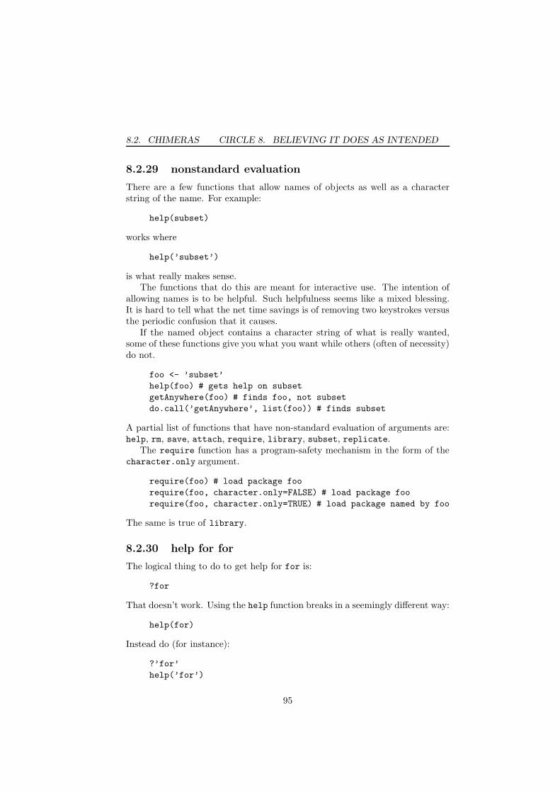
8.2. CHIMERAS CIRCLE 8. BELIEVING IT DOES AS INTENDED
8.2.29 nonstandard evaluation
There are a few functions that allow names of objects as well as a characterstring of the name. For example:
help(subset)
works where
help(’subset’)
is what really makes sense.The functions that do this are meant for interactive use. The intention of
allowing names is to be helpful. Such helpfulness seems like a mixed blessing.It is hard to tell what the net time savings is of removing two keystrokes versusthe periodic confusion that it causes.
If the named object contains a character string of what is really wanted,some of these functions give you what you want while others (often of necessity)do not.
foo <- ’subset’
help(foo) # gets help on subset
getAnywhere(foo) # finds foo, not subset
do.call(’getAnywhere’, list(foo)) # finds subset
A partial list of functions that have non-standard evaluation of arguments are:help, rm, save, attach, require, library, subset, replicate.
The require function has a program-safety mechanism in the form of thecharacter.only argument.
require(foo) # load package foo
require(foo, character.only=FALSE) # load package foo
require(foo, character.only=TRUE) # load package named by foo
The same is true of library.
8.2.30 help for for
The logical thing to do to get help for for is:
?for
That doesn’t work. Using the help function breaks in a seemingly different way:
help(for)
Instead do (for instance):
?’for’
help(’for’)
95
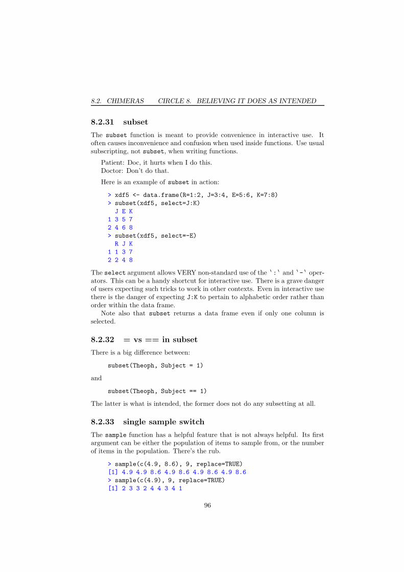
8.2. CHIMERAS CIRCLE 8. BELIEVING IT DOES AS INTENDED
8.2.31 subset
The subset function is meant to provide convenience in interactive use. Itoften causes inconvenience and confusion when used inside functions. Use usualsubscripting, not subset, when writing functions.
Patient: Doc, it hurts when I do this.Doctor: Don’t do that.
Here is an example of subset in action:
> xdf5 <- data.frame(R=1:2, J=3:4, E=5:6, K=7:8)
> subset(xdf5, select=J:K)
J E K
1 3 5 7
2 4 6 8
> subset(xdf5, select=-E)
R J K
1 1 3 7
2 2 4 8
The select argument allows VERY non-standard use of the 8 : 8 and 8 - 8 oper-ators. This can be a handy shortcut for interactive use. There is a grave dangerof users expecting such tricks to work in other contexts. Even in interactive usethere is the danger of expecting J:K to pertain to alphabetic order rather thanorder within the data frame.
Note also that subset returns a data frame even if only one column isselected.
8.2.32 = vs == in subset
There is a big difference between:
subset(Theoph, Subject = 1)
and
subset(Theoph, Subject == 1)
The latter is what is intended, the former does not do any subsetting at all.
8.2.33 single sample switch
The sample function has a helpful feature that is not always helpful. Its firstargument can be either the population of items to sample from, or the numberof items in the population. There’s the rub.
> sample(c(4.9, 8.6), 9, replace=TRUE)
[1] 4.9 4.9 8.6 4.9 8.6 4.9 8.6 4.9 8.6
> sample(c(4.9), 9, replace=TRUE)
[1] 2 3 3 2 4 4 3 4 1
96

8.2. CHIMERAS CIRCLE 8. BELIEVING IT DOES AS INTENDED
If the population is numeric, at least 1 and of size one (due, say, to selectionwithin a function), then it gets interpreted as the size of the population. Notein the example above the size is rounded down to the nearest integer.
There is a kludgy workaround, which is to make the population character:
> as.numeric(sample(as.character(c(4.9)), 9, replace=TRUE))
[1] 4.9 4.9 4.9 4.9 4.9 4.9 4.9 4.9 4.9
8.2.34 changing names of pieces
R does an extraordinary job of ferreting out replacement statements. For ex-ample, the following actually does what is intended:
names(mylist$b[[1]]) <- letters[1:10]
It is possible to get it wrong though. Here is an example:
> right <- wrong <- c(a=1, b=2)
> names(wrong[1]) <- ’changed’
> wrong
a b
1 2
> names(right)[1] <- ’changed’
> right
changed b
1 2
What goes wrong is that we change names on something that is then thrownaway. So to change the first two names in our ridiculous example, we would do:
names(mylist$b[[1]])[1:2] <- LETTERS[1:2]
8.2.35 a puzzle
> class(dfxy)
[1] "data.frame"
> length(dfxy)
[1] 8
> length(as.matrix(dfxy))
[1] 120
What is
nrow(dfxy)
97

8.2. CHIMERAS CIRCLE 8. BELIEVING IT DOES AS INTENDED
8.2.36 another puzzle
If the following is a valid command:
weirdFun()()()
what does weirdFun return?Write an example.
8.2.37 data frames vs matrices
A matrix and a data frame look the same when printed. That is good—they areconceptually very similar. However, they are implemented entirely differently.
Objects that are conceptually similar but implemented differently are a goodsource of confusion.
> x %*% y
Error in x %*% y : requires numeric matrix/vector arguments
The problem here is that while x looks like a matrix, it is actually a data frame.A solution is to use as.matrix, or possibly data.matrix,
In theory the actual implementation of data frames should not matter at allto the user. Theory often has some rough edges.
8.2.38 apply not for data frames
One rough edge is applying a function to a data frame. The apply functionoften doesn’t do what is desired because it coerces the data frame to a matrixbefore proceeding.
apply(myDataFrame, 2, class) # not right
Data frames are actually implemented as a list with each component of the listbeing a column of the data frame. Thus:
lapply(myDataFrame, class)
does what was attempted above.
8.2.39 data frames vs matrices (reprise)
Consider the command:
array(sample(x), dim(x))
This permutes the elements of a matrix. If x is a data frame, the command willwork but the result will most assuredly not be what you want.
It is possible to get a column of a data frame with a command like:
98
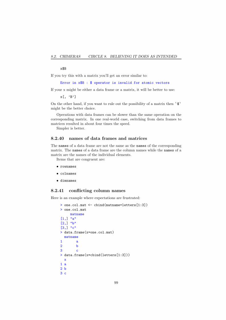
8.2. CHIMERAS CIRCLE 8. BELIEVING IT DOES AS INTENDED
x$B
If you try this with a matrix you’ll get an error similar to:
Error in x$B : $ operator is invalid for atomic vectors
If your x might be either a data frame or a matrix, it will be better to use:
x[, ’B’]
On the other hand, if you want to rule out the possibility of a matrix then 8 $ 8
might be the better choice.
Operations with data frames can be slower than the same operation on thecorresponding matrix. In one real-world case, switching from data frames tomatrices resulted in about four times the speed.
Simpler is better.
8.2.40 names of data frames and matrices
The names of a data frame are not the same as the names of the correspondingmatrix. The names of a data frame are the column names while the names of amatrix are the names of the individual elements.
Items that are congruent are:
• rownames
• colnames
• dimnames
8.2.41 conflicting column names
Here is an example where expectations are frustrated:
> one.col.mat <- cbind(matname=letters[1:3])
> one.col.mat
matname
[1,] "a"
[2,] "b"
[3,] "c"
> data.frame(x=one.col.mat)
matname
1 a
2 b
3 c
> data.frame(x=cbind(letters[1:3]))
x
1 a
2 b
3 c
99

8.2. CHIMERAS CIRCLE 8. BELIEVING IT DOES AS INTENDED
When the call to data.frame uses a tag (name) for an item, it is expected thatthe corresponding column of the output will have that name. However, columnnames that are already there take precedence.
Notice also that the data frames contain a factor column rather than char-acter.
8.2.42 cbind favors matrices
If you cbind two matrices, you get a matrix. If you cbind two data frames, youget a data frame. If you cbind two vectors, you get a matrix:
> is.matrix(cbind(x=1:10, y=rnorm(10)))
[1] TRUE
If you want a data frame, then use the data.frame function:
> dfxy <- data.frame(x=1:10, y=rnorm(10))
8.2.43 data frame equal number of rows
A data frame is implemented as a list. But not just any list will do—eachcomponent must represent the same number of rows. If you work hard enough,you might be able to produce a data frame that breaks the rule. More likelyyour frustration will be that R stops you from getting to such an absurd result.
8.2.44 matrices in data frames
Let’s make two data frames:
> ymat <- array(1:6, c(3,2))
> xdf6 <- data.frame(X=101:103, Y=ymat)
> xdf7 <- data.frame(X=101:103)
> xdf7$Y <- ymat
> xdf6
X Y.1 Y.2
1 101 1 4
2 102 2 5
3 103 3 6
> xdf7
X Y.1 Y.2
1 101 1 4
2 102 2 5
3 103 3 6
> dim(xdf6)
[1] 3 3
> dim(xdf7)
[1] 3 2
100
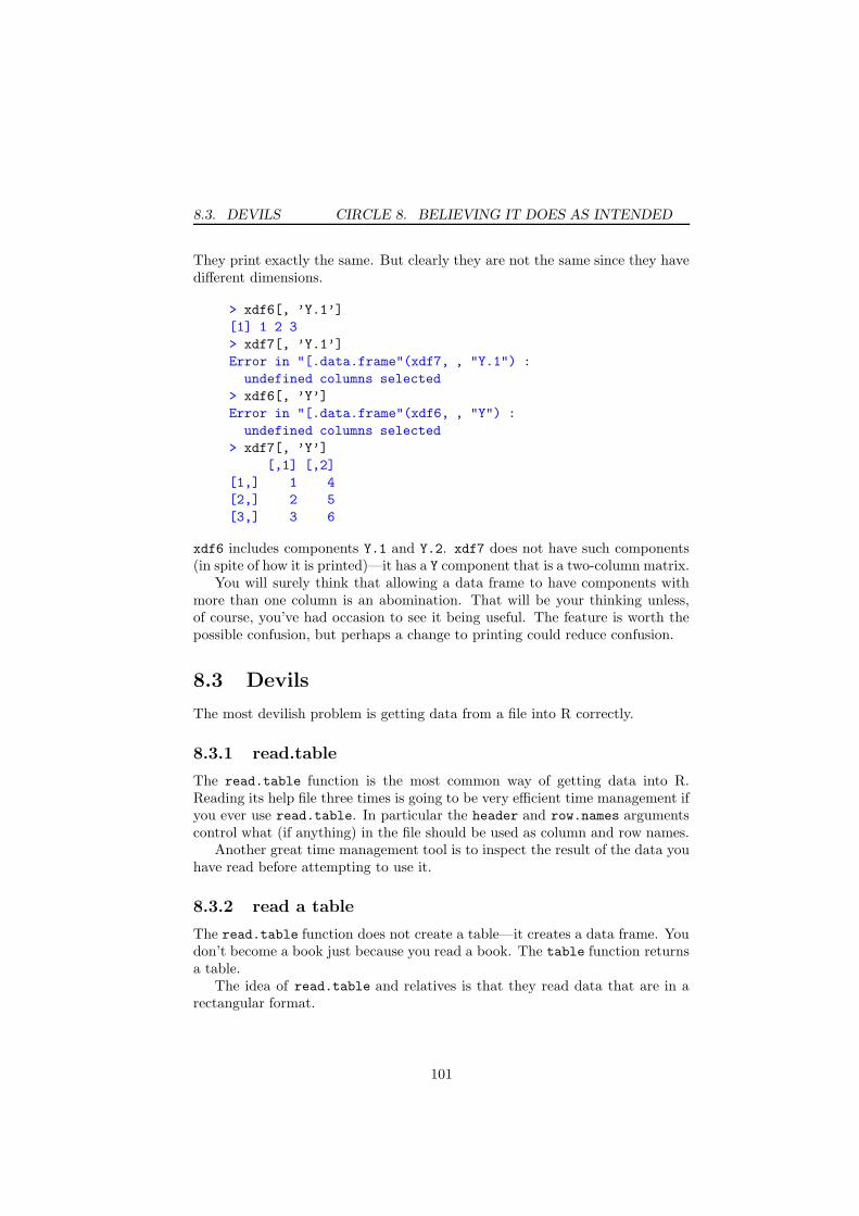
8.3. DEVILS CIRCLE 8. BELIEVING IT DOES AS INTENDED
They print exactly the same. But clearly they are not the same since they havedifferent dimensions.
> xdf6[, ’Y.1’]
[1] 1 2 3
> xdf7[, ’Y.1’]
Error in "[.data.frame"(xdf7, , "Y.1") :
undefined columns selected
> xdf6[, ’Y’]
Error in "[.data.frame"(xdf6, , "Y") :
undefined columns selected
> xdf7[, ’Y’]
[,1] [,2]
[1,] 1 4
[2,] 2 5
[3,] 3 6
xdf6 includes components Y.1 and Y.2. xdf7 does not have such components(in spite of how it is printed)—it has a Y component that is a two-column matrix.
You will surely think that allowing a data frame to have components withmore than one column is an abomination. That will be your thinking unless,of course, you’ve had occasion to see it being useful. The feature is worth thepossible confusion, but perhaps a change to printing could reduce confusion.
8.3 Devils
The most devilish problem is getting data from a file into R correctly.
8.3.1 read.table
The read.table function is the most common way of getting data into R.Reading its help file three times is going to be very efficient time management ifyou ever use read.table. In particular the header and row.names argumentscontrol what (if anything) in the file should be used as column and row names.
Another great time management tool is to inspect the result of the data youhave read before attempting to use it.
8.3.2 read a table
The read.table function does not create a table—it creates a data frame. Youdon’t become a book just because you read a book. The table function returnsa table.
The idea of read.table and relatives is that they read data that are in arectangular format.
101

8.3. DEVILS CIRCLE 8. BELIEVING IT DOES AS INTENDED
8.3.3 the missing, the whole missing and nothing but themissing
Misreading missing values is an efficacious way of producing garbage. Missingvalues can become non-missing, non-missing values can become missing, logi-cally numeric columns can become factors.
The na.strings argument to read.table needs to be set properly. Anexample might be:
na.strings=c(’.’, ’-999’)
8.3.4 misquoting
A quite common file format is to have a column of names followed by somenumber of columns of data. If there are any apostrophes in those names, thenyou are likely to get an error reading the file unless you have set the quote
argument to read.table. A likely value for quote is:
quote=’’
This sounds like easy advise, but almost surely it is not going to be apparentthat quotes are the problem. You may get an error that says there was thewrong number of items in a line. When you get such an error, it is often agood idea to use count.fields to get a sense of what R thinks about your file.Something along the lines of:
foo.cf <- count.fields(’foo.txt’, sep=’\t’)table(foo.cf)
8.3.5 thymine is TRUE, female is FALSE
You are reading in DNA bases identified as A, T, G and C. The columns areread as factors. Except for the column that is all T—that column is logical.
Similarly, a column for gender that is all F for female will be logical.
The solution is to use the read.table argument:
colClasses=’character’
or
colClasses=’factor’
as you like.If there are columns of other sorts of data, then you need to give colClasses
a vector of appropriate types for the columns in the file.Using colClasses can also make the call much more efficient.
102

8.3. DEVILS CIRCLE 8. BELIEVING IT DOES AS INTENDED
Figure 8.3: The treacherous to country and the treacherous to guests and hostsby Sandro Botticelli.
103

8.3. DEVILS CIRCLE 8. BELIEVING IT DOES AS INTENDED
8.3.6 whitespace is white
Whitespace is invisible, and we have a predilection to believe that invisiblemeans non-existent.
> factor(c(’A ’, ’A’, ’B’))
[1] A A B
Levels: A A B
It is extraordinarily easy to get factors like this when reading in data. Settingthe strip.white argument of read.table to TRUE can prevent this.
8.3.7 extraneous fields
When a file has been created in a spreadsheet, there are sometimes extraneousempty fields in some of the lines of the file. In such a case you might get anerror similar to:
> mydat <- read.table(’myfile’, header=TRUE, sep=’\t’)Error in scan(file, what, nmax, sep, dec, quote, skip, :
line 10 did not have 55 elements
This, of course, is a perfect instance to use count.fields to see what is goingon. If extraneous empty fields do seem to be the problem, then one solution is:
> mydat <- read.table(’myfile’, header=TRUE, sep=’\t’,+ fill=TRUE)
> mydat <- mydat[, 1:53]
At this point, it is wiser than usual to carefully inspect the results to see thatthe data are properly read and aligned.
8.3.8 fill and extraneous fields
When the fill argument is TRUE (which is the default for read.csv andread.delim but not for read.table), there can be trouble if there is a variablenumber of fields in the file.
> writeLines(c("A,B,C,D",
+ "1,a,b,c",
+ "2,d,e,f",
+ "3,a,i,j",
+ "4,a,b,c",
+ "5,d,e,f",
+ "6,g,h,i,j,k,l,m,n"),
+ con=file("test.csv"))
> read.csv("test.csv")
A B C D
104
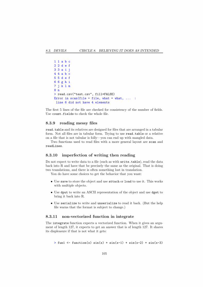
8.3. DEVILS CIRCLE 8. BELIEVING IT DOES AS INTENDED
1 1 a b c
2 2 d e f
3 3 a i j
4 4 a b c
5 5 d e f
6 6 g h i
7 j k l m
8 n
> read.csv("test.csv", fill=FALSE)
Error in scan(file = file, what = what, ... :
line 6 did not have 4 elements
The first 5 lines of the file are checked for consistency of the number of fields.Use count.fields to check the whole file.
8.3.9 reading messy files
read.table and its relatives are designed for files that are arranged in a tabularform. Not all files are in tabular form. Trying to use read.table or a relativeon a file that is not tabular is folly—you can end up with mangled data.
Two functions used to read files with a more general layout are scan andreadLines.
8.3.10 imperfection of writing then reading
Do not expect to write data to a file (such as with write.table), read the databack into R and have that be precisely the same as the original. That is doingtwo translations, and there is often something lost in translation.
You do have some choices to get the behavior that you want:
• Use save to store the object and use attach or load to use it. This workswith multiple objects.
• Use dput to write an ASCII representation of the object and use dget tobring it back into R.
• Use serialize to write and unserialize to read it back. (But the helpfile warns that the format is subject to change.)
8.3.11 non-vectorized function in integrate
The integrate function expects a vectorized function. When it gives an argu-ment of length 127, it expects to get an answer that is of length 127. It sharesits displeasure if that is not what it gets:
> fun1 <- function(x) sin(x) + sin(x-1) + sin(x-2) + sin(x-3)
105

8.3. DEVILS CIRCLE 8. BELIEVING IT DOES AS INTENDED
> integrate(fun1, 0, 2)
-1.530295 with absolute error < 2.2e-14
> fun2 <- function(x) sum(sin(x - 0:3))
> integrate(fun2, 0, 2)
Error in integrate(fun2, 0, 2) :
evaluation of function gave a result of wrong length
In addition: Warning message:
longer object length
is not a multiple of shorter object length in: x - 0:3
> fun3 <- function(x) rowSums(sin(outer(x, 0:3, ’-’)))
> integrate(fun3, 0, 2)
-1.530295 with absolute error < 2.2e-14
fun1 is a straightforward implementation of what was wanted, but not easyto generalize. fun2 is an ill-conceived attempt at mimicking fun1. fun3 isa proper implementation of the function using outer as a step in getting thevectorization correct.
8.3.12 non-vectorized function in outer
The function given to outer needs to be vectorized (in the usual sense):
> outer(1:3, 4:1, max)
Error in dim(robj) <- c(dX, dY) :
dims [product 12] do not match the length of object [1]
> outer(1:3, 4:1, pmax)
[,1] [,2] [,3] [,4]
[1,] 4 3 2 1
[2,] 4 3 2 2
[3,] 4 3 3 3
> outer(1:3, 4:1, Vectorize(function(x, y) max(x, y)))
[,1] [,2] [,3] [,4]
[1,] 4 3 2 1
[2,] 4 3 2 2
[3,] 4 3 3 3
The Vectorize function can be used to transform a function (by essentiallyadding a loop—it contains no magic to truly vectorize the function).
8.3.13 ignoring errors
You have a loop in which some of the iterations may produce an error. Youwould like to ignore any errors and proceed with the loop. One solution is touse try.
The code:
106

8.3. DEVILS CIRCLE 8. BELIEVING IT DOES AS INTENDED
ans <- vector(’list’, n)
for(i in seq(length.out=n)) {ans[[i]] <- rpois(round(rnorm(1, 5, 10)), 10)
}
will fail when the number of Poisson variates requested is negative. This can bemodified to:
ans <- vector(’list’, n)
for(i in seq(length.out=n)) {this.ans <- try(rpois(round(rnorm(1, 5, 10)), 10))
if(!inherits(this.ans, ’try-error’)) {ans[[i]] <- this.ans
}}
Another approach is to use tryCatch rather than try:
ans <- vector(’list’, n)
for(i in seq(length.out=n)) {ans[[i]] <- tryCatch(rpois(round(rnorm(1, 5, 10)), 10),
error=function(e) NaN)
}
8.3.14 accidentally global
It is possible for functions to work where they are created, but not to work ingeneral. Objects within the function can be global accidentally.
> myfun4 <- function(x) x + y
> myfun4(30)
[1] 132
> rm(y)
> myfun4(30)
Error in myfun4(30) : Object "y" not found
The findGlobals function can highlight global objects:
> library(codetools)
> findGlobals(myfun4)
[1] "+" "y"
8.3.15 handling ...
The 8 ... 8 construct can be a slippery thing to get hold of until you know thetrick. One way is to package it into a list:
107
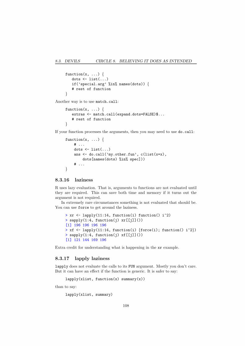
8.3. DEVILS CIRCLE 8. BELIEVING IT DOES AS INTENDED
function(x, ...) {dots <- list(...)
if(’special.arg’ %in% names(dots)) {# rest of function
}Another way is to use match.call:
function(x, ...) {extras <- match.call(expand.dots=FALSE)$...
# rest of function
}If your function processes the arguments, then you may need to use do.call:
function(x, ...) {# ...
dots <- list(...)
ans <- do.call(’my.other.fun’, c(list(x=x),
dots[names(dots) %in% spec]))
# ...
}
8.3.16 laziness
R uses lazy evaluation. That is, arguments to functions are not evaluated untilthey are required. This can save both time and memory if it turns out theargument is not required.
In extremely rare circumstances something is not evaluated that should be.You can use force to get around the laziness.
> xr <- lapply(11:14, function(i) function() i^2)
> sapply(1:4, function(j) xr[[j]]())
[1] 196 196 196 196
> xf <- lapply(11:14, function(i) {force(i); function() i^2})> sapply(1:4, function(j) xf[[j]]())
[1] 121 144 169 196
Extra credit for understanding what is happening in the xr example.
8.3.17 lapply laziness
lapply does not evaluate the calls to its FUN argument. Mostly you don’t care.But it can have an effect if the function is generic. It is safer to say:
lapply(xlist, function(x) summary(x))
than to say:
lapply(xlist, summary)
108
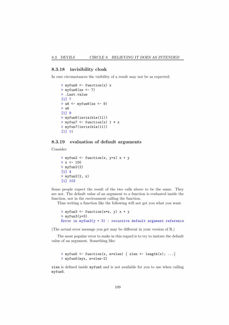
8.3. DEVILS CIRCLE 8. BELIEVING IT DOES AS INTENDED
8.3.18 invisibility cloak
In rare circumstances the visibility of a result may not be as expected:
> myfun6 <- function(x) x
> myfun6(zz <- 7)
> .Last.value
[1] 7
> a6 <- myfun6(zz <- 9)
> a6
[1] 9
> myfun6(invisible(11))
> myfun7 <- function(x) 1 * x
> myfun7(invisible(11))
[1] 11
8.3.19 evaluation of default arguments
Consider:
> myfun2 <- function(x, y=x) x + y
> x <- 100
> myfun2(2)
[1] 4
> myfun2(2, x)
[1] 102
Some people expect the result of the two calls above to be the same. Theyare not. The default value of an argument to a function is evaluated inside thefunction, not in the environment calling the function.
Thus writing a function like the following will not get you what you want.
> myfun3 <- function(x=x, y) x + y
> myfun3(y=3)
Error in myfun3(y = 3) : recursive default argument reference
(The actual error message you get may be different in your version of R.)
The most popular error to make in this regard is to try to imitate the defaultvalue of an argument. Something like:
> myfun5 <- function(x, n=xlen) { xlen <- length(x); ...}> myfun5(myx, n=xlen-2)
xlen is defined inside myfun5 and is not available for you to use when callingmyfun5.
109

8.3. DEVILS CIRCLE 8. BELIEVING IT DOES AS INTENDED
8.3.20 sapply simplification
The sapply function “simplifies” the output of lapply. It isn’t always so simple.That is, the simplification that you get may not be the simplification you expect.This uncertainty makes sapply not so suitable for use inside functions. Thevapply function is sometimes a safer alternative.
8.3.21 one-dimensional arrays
Arrays can be of any positive dimension (modulo memory and vector lengthlimits). In particular, one-dimensional arrays are possible. Almost always theselook and act like plain vectors. Almost.
Here is an example where they don’t:
> df2 <- data.frame(x=rep(1, 3), y=tapply(1:9,
+ factor(rep(c(’A’, ’B’, ’C’), each=3)), sum))
> df2
x y
A 1 6
B 1 15
C 1 24
> tapply(df2$y, df2$x, length)
1
3
> by(df2$y, df2$x, length)
INDICES: 1
[1] 1
> by(as.vector(df2$y), df2$x, length)
INDICES: 1
[1] 3
tapply returns an array, in particular it can return a one-dimensional array—which is the case with df2$y. The by function in this case when given a one-dimensional array produces the correct answer to a question that we didn’tthink we were asking.
One-dimensional arrays are neither matrices nor (exactly) plain vectors.
8.3.22 by is for data frames
The by function is essentially just a pretty version of tapply for data frames.The “for data frames” is an important restriction. If the first argument of yourcall to by is not a data frame, you may be in for trouble.
> tapply(array(1:24, c(2,3,4)), 1:24 %% 2, length)
0 1
12 12
> by(array(1:24, c(2,3,4)), 1:24 %% 2, length)
110
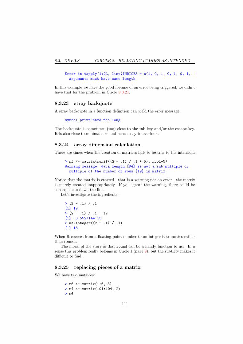
8.3. DEVILS CIRCLE 8. BELIEVING IT DOES AS INTENDED
Error in tapply(1:2L, list(INDICES = c(1, 0, 1, 0, 1, 0, 1, :
arguments must have same length
In this example we have the good fortune of an error being triggered, we didn’thave that for the problem in Circle 8.3.21.
8.3.23 stray backquote
A stray backquote in a function definition can yield the error message:
symbol print-name too long
The backquote is sometimes (too) close to the tab key and/or the escape key.It is also close to minimal size and hence easy to overlook.
8.3.24 array dimension calculation
There are times when the creation of matrices fails to be true to the intention:
> mf <- matrix(runif((2 - .1) / .1 * 5), ncol=5)
Warning message: data length [94] is not a sub-multiple or
multiple of the number of rows [19] in matrix
Notice that the matrix is created—that is a warning not an error—the matrixis merely created inappropriately. If you ignore the warning, there could beconsequences down the line.
Let’s investigate the ingredients:
> (2 - .1) / .1
[1] 19
> (2 - .1) / .1 - 19
[1] -3.552714e-15
> as.integer((2 - .1) / .1)
[1] 18
When R coerces from a floating point number to an integer it truncates ratherthan rounds.
The moral of the story is that round can be a handy function to use. In asense this problem really belongs in Circle 1 (page 9), but the subtlety makes itdifficult to find.
8.3.25 replacing pieces of a matrix
We have two matrices:
> m6 <- matrix(1:6, 3)
> m4 <- matrix(101:104, 2)
> m6
111

8.3. DEVILS CIRCLE 8. BELIEVING IT DOES AS INTENDED
[,1] [,2]
[1,] 1 4
[2,] 2 5
[3,] 3 6
> m4
[,1] [,2]
[1,] 101 103
[2,] 102 104
Our task is to create a new matrix similar to m6 where some of the rows arereplaced by the first row of m4. Here is the natural thing to do:
> m6new <- m6
> m6new[c(TRUE, FALSE, TRUE), ] <- m4[1,]
> m6new
[,1] [,2]
[1,] 101 101
[2,] 2 5
[3,] 103 103
We are thinking about rows being the natural way of looking at the problem.The problem is that that isn’t the R way, despite the context.
One way of getting what we want is:
> s6 <- c(TRUE, FALSE, TRUE)
> m6new[s6, ] <- rep(m4[1,], each=sum(s6))
> m6new
[,1] [,2]
[1,] 101 103
[2,] 2 5
[3,] 101 103
8.3.26 reserved words
R is a language. Because of this, there are reserved words that you can not useas object names. Perhaps you can imagine the consequences if the followingcommand actually worked:
FALSE <- 4
You can see the complete list of reserved words with:
?Reserved
8.3.27 return is a function
Unlike some other languages return is a function that takes the object meantto be returned. The following construct does NOT do what is intended:
112

8.3. DEVILS CIRCLE 8. BELIEVING IT DOES AS INTENDED
return (2/5) * 3:9
It will return 0.4 and ignore the rest.
8.3.28 return is a function (still)
return is a function and not a reserved word.
> # kids, don’t try this at home
> return <- function(x) 4 * x
> # notice: no error
> rm(return)
8.3.29 BATCH failure
Friday afternoon you start off a batch job happy in the knowledge that comeMonday morning you will have the results of sixty-some hours of computationin your hands. Come Monday morning results are nowhere to be found. Thejob fell over after an hour because of a stray comma in your file of commands.
Results can’t be guaranteed, but it is possible to at least test for that straycomma and its mates. Once you’ve written your file of commands, parse thefile:
parse(file=’batchjob.in’)
If there is a syntax error in the file, then you’ll get an error and a location forthe (first) error. If there are no syntax errors, then you’ll get an expression (alarge expression).
8.3.30 corrupted .RData
There are times when R won’t start in a particular location because of a cor-rupted .RData file. If what you have in the .RData is important, this is badnews.
Sometimes this can be caused by a package not being attached in the Rsession that the file depends on. Whether or not this is the problem, you cantry starting R in vanilla mode (renaming the .RData file first is probably a goodidea) and then try attaching the file.
In principle it should be possible to see what objects a .RData file holds andextract a selection of objects from it. However, I don’t know of any tools to dothat.
8.3.31 syntax errors
Syntax errors are one of the most common problems, especially for new users.Unfortunately there is no good way to track down the problem other than
113
8.3. DEVILS CIRCLE 8. BELIEVING IT DOES AS INTENDED
puzzling over it. The most common problems are mismatched parentheses orsquare brackets, and missing commas.
Using a text editor that performs syntax highlighting can eliminate a lot ofthe problems.
Here is a particularly nasty error:
> lseq <- seq(0, 1, 1ength=10)
Error: unexpected input in "seq(0, 1, 1en"
Hint: the end of the error message is the important location. In fact, the lastletter that it prints is the first point at which it knew something was wrong.
8.3.32 general confusion
If you are getting results that are totally at odds with your expectations, lookwhere you are stepping:
• Objects may be different than you expect. You can use str to diagnosethis possibility. (The output of str may not make much sense immedi-ately, but a little study will reveal what it is saying.)
• Functions may be different than you expect. Try using conflicts todiagnose this.
• Pretty much the only thing left is your expectations.
Calls to browser, cat and debugger can help you eliminate ghosts, chimerasand devils. But the most powerful tool is your skepticism.
114
Circle 9
Unhelpfully Seeking Help
Here live the thieves, guarded by the centaur Cacus. The inhabitants are bittenby lizards and snakes.
There’s a special place for those who—not being content with one of the 8Circles we’ve already visited—feel compelled to drag the rest of us into hell.
The road to writing a mail message should include at least the followingstops:
9.1 Read the appropriate documentation.
“RTFM” in the jargon. There is a large amount of documentation about R, bothofficial and contributed, and in various formats. A large amount of documenta-tion means that it is often nontrivial to find what you are looking for—especiallywhen frustration is setting in and blood pressure is rising.
Breathe.
There are various searches that you can do. R functions for searching includehelp.search, RSiteSearch and apropos.
If you are looking for particular functionality, then check the Task Views(found on the left-side menu of CRAN).
If you have an error, then look in rather than out—debug the problem.One way of debugging is to set the error option, and then use the debugger
function:
options(error=dump.frames)
# command that causes the error
debugger()
The debugger function then provides a menu of the stack of functions that havebeen called at the point of the error. You can inspect the state of the objectsinside these functions, and hopefully understand what the problem is.
115
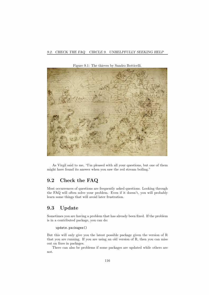
9.2. CHECK THE FAQ CIRCLE 9. UNHELPFULLY SEEKING HELP
Figure 9.1: The thieves by Sandro Botticelli.
As Virgil said to me, “I’m pleased with all your questions, but one of themmight have found its answer when you saw the red stream boiling.”
9.2 Check the FAQ
Most occurrences of questions are frequently asked questions. Looking throughthe FAQ will often solve your problem. Even if it doesn’t, you will probablylearn some things that will avoid later frustration.
9.3 Update
Sometimes you are having a problem that has already been fixed. If the problemis in a contributed package, you can do:
update.packages()
But this will only give you the latest possible package given the version of Rthat you are running. If you are using an old version of R, then you can missout on fixes in packages.
There can also be problems if some packages are updated while others arenot.
116
9.4. POSTINGGUIDE CIRCLE 9. UNHELPFULLY SEEKING HELP
9.4 Read the posting guide
This will give you another point of view about how to approach the remainingsteps. In particular, it will instruct you on what types of questions belong onthe various mailing lists.
Another good resource (not specific to R, but apropos) is a web page called“How to ask questions the smart way”.
If you have faithfully performed the tasks up to here, you probably do notneed to continue. But do continue if it is warranted.
You can do:
help.request()
on some platforms. This will create a file containing some of the importantinformation that should be in the message. It also reminds you of steps thatyou should take.
9.5 Select the best list
Your choices are R-help, R-devel and the special interest groups. Or the Bio-conductor list if your question relates to a Bioconductor package.
Pick one—cross posting is seriously discouraged.
There are some topics that should definitely be sent to a special interestgroup. For example, questions about garch should go to R-sig-finance. No oneoutside of finance knows about garch, nor will they ever. Non-finance peoplehave no alternative but to think that a garch is someone who lives in Garching.Garch is a specifically financial model.
Sending the question to the right list is in everyone’s best interest. If yousend a question about garch to R-help, then:
• Some of the people most qualified to answer your question will not see it(my guess is that the vast majority of subscribers to R-sig-finance do notsubscribe to R-help).
• There will be thousands of people for whom the question will be a completewaste of time.
• There will be people in the special interest group who could profit fromthe answers, but who will never see the answers.
If the functionality you are concerned with is from a contributed package, seri-ously consider writing only to the maintainer of the package. Should you deemit appropriate to write to a list, then certainly say what package or packagesare involved.
117
9.6. SUBJECTLINE CIRCLE 9. UNHELPFULLY SEEKING HELP
Do NOT file a bug report unless you are absolutely sure it is a bug—bugreports entail additional work on the part of R Core. If the behavior is discussedin this document, it is not a bug. Just because something doesn’t work on yourmachine, that does not mean it is a problem in R. If there is a question markin your statement (or your mind), it is not (yet) a bug. It can not be a bug ifyou do not have a reproducible method of exhibiting the behavior. It is a bugif you have a well-reasoned argument of why the current behavior is bad, it isnot documented to have the current behavior, and you have a patch to fix theproblem. Patches are highly appreciated. Note that “current behavior” meansthe buggy behavior needs to be exhibited in the development version of R—donot consider it enough to only check whatever version of R you happen to berunning. Also check to make sure the bug has not already been reported.
Even if it is clearly a bug, it may be inappropriate to file an R bug report.The bug need not be in R, but may be in some other piece of software. If in anydoubt, send a message to R-devel instead. In particular do not file an R bugreport for a contributed package—send your message to the package maintainer.
Another do not: Do not hijack an existing thread. That will make a messfor people viewing the list by threads. Make a new message addressed to thelist.
9.6 Use a descriptive subject line
Recall what words you used to search the archives (which you did do) to tryto find an answer to your problem, and use a selection of those. Subjects like“Problem with code” and “Help!!” are less than perfect. A legacy of your mailshould be to improve things for other users—that is unlikely to happen withoutan explicit subject line.
With an appropriate subject, more of the right people will read your messageand hence be in a position to give you an answer.
Do not include words like “urgent”. The help you receive on the mailinglists is a gift, not a right. Being pushy is likely to engender worse service, notbetter service.
At the other end of the message there is room for your identity. Some peoplerefuse to respond to anonymous messages. I find it hard to believe that manypeople refuse to respond to a message because the sender is identified. So onbalance you may get better response if you identify yourself.
9.7 Clearly state your question
A statement like:
When I use function blahblah, it doesn’t work.
118

9.7. CLEARLY STATE CIRCLE 9. UNHELPFULLY SEEKING HELP
Figure 9.2: The thieves by Sandro Botticelli.
is not a clear statement of your question. We don’t know what “use” means,we don’t know what you expect “work” to look like, and we don’t know what“doesn’t work” means.
Explain:
• What function you are using (for example, there are a number of garchimplementations—you need to say which one you are using).
• What you want.
• What you expected.
• Show us what happened.
• Show us the output of str on your data.
Sometimes background on why you are asking the question is relevant. Considerthe question:
Is there a way to order pizza with R?
The answer is, of course, “Of course there is a way to order pizza. This *is*R.”
119

9.8. EXAMPLE CIRCLE 9. UNHELPFULLY SEEKING HELP
The question lacks both specificity and background (though it is mercifullybrief). The answer to how to do the operation could depend on whether youwant it delivered, and what size it should be. And do you want anchovies? Ifyou provide background, you may get an answer that proposes a better—butentirely different—way of getting nutrients into your bloodstream.
Do not confuse a warning with an error. There are two differences:
1. warnings say “warning” and errors say “error”.
2. the computation continues when there is a warning but is interruptedwhen there is an error.
If there really is an error, then give the results of:
traceback()
The word “crash” is very ambiguous. It would be better if you didn’t use theword at all. If you do use it, you need to explain exactly what you mean. Inaddition to avoiding the use of vague words like “crash”, you can be informativeby displaying the results of sessionInfo().
If error or warning messages are not in English and you are writing to anEnglish mailing list, then translating pertinent messages would be in your bestinterest. But do show the real message as well.
If you are asking if method XYZ is implemented in R, then say that XYZstands for Xeric Yare Zeugma (and hence not X-raY Zoometry). Give a briefexplanation and a reference (preferably available online). The same technique,or something suitably similar, may well go by a different name.
Did I say you should give the results of sessionInfo()? The more infor-mation about the version of R you are using and your machine, the better. Ifthe information is accurate, that’s a plus.
9.8 Give a minimal, self-contained example
Note this does not say, “Give an example.” It says to give a minimal, self-contained example. A minimal, self-contained example allows readers to repro-duce the problem easily. The easier you make it for your readers, the more likelyyou receive help.
The word “minimal” implies an optimization. Elements of that optimizationinclude:
• Minimize the number of packages involved. Ideal is if a vanilla sessionsuffices.
• Minimize the number of functions involved.
• Minimize the size of any functions that are yours.
120

9.9. WAIT CIRCLE 9. UNHELPFULLY SEEKING HELP
• Minimize the number and size of datasets involved. If peculiar data arerequired and your data are complicated, large and/or proprietary, thenmake up some data that exhibits the problem.
Often the process of making a minimal example reveals the problem. If theproblem does not reveal itself, then keep these hints in mind:
• Make your example easy to cut and paste. The dput function is sometimesuseful for this.
• If the example involves random numbers, then use set.seed to make thenumbers non-random.
• Using data that comes with R is often the easiest for your readers.
• Format the code to be easy to understand—the space bar is an excellentresource.
Your minimal, self-contained example should never ever include a line of codelike:
rm(list=ls())
There’s a special special place for those who try to lull their would-be helpersinto destroying their data.
It can not be emphasized enough that a message is putting yourself at themercy of strangers. If someone has the wit and knowledge to answer yourquestion, they probably have other things they would like to do. Making yourmessage clear, concise and user-friendly gives you the best hope of at least oneof those strangers diverting their attention away from their life towards yourproblem.
9.9 Wait
Don’t send the message immediately. Wait some amount of time—at least 1hour, at most 1.7348 days. Leave the room you’re in.
Now reread the message from a typical list member’s point of view. Theanswer may become apparent. More likely you may see how the question couldbe made more clear. Add information that only you know but which the messageassumes the reader knows. Imagine yourself going through all of the steps ofyour problem from the beginning.
Send the message in plain text, not html.Only send the message once. Just because you don’t immediately see your
message on the list does not mean it didn’t go through. Seeing the same messagemultiple times annoys people and reduces the chances they will answer you.There seems to be positive correlation between a person’s level of annoyance atthis and ability to answer questions.
121

Postscript
irgil and I came upon the road leading to the bright world. We climbedthrough an opening to see once again the stars.
Most of this was stolen from the archives of R-help (thieves are consigned toCircle 9 [page 115], as you’ll recall). Thanks go to Tim Triche, Jr. and especiallyMark Difford for help with the table of contents and the index, and for well-placed prods. Mark’s version of the source document went through an infernoof its own.
What spark of life there may be in these scribblings is due largely to the con-tributors of R-help, and to Beatrice.
122

Index
1-D arrays, 110tapply, 110
Assignment operators, 94Attributes, see Objects, S3 methods,
S4 methods
Backslashed characters, see Table 8.1Braces, curly, 28Breathe, 115
Calculating products, see Vectorizationsafe, efficient calculation, 18
Capitalization, 46, 78Circle I, 9–11
virtuous pagans, floating point andall that, 9
Circle III, 17–23cold, dead weight of the past, 17foreign tongues, 17pain and pleasure of perfection, 17
Complex numbers, 94Computing on the language, 32Corrupted .RData, 113Curly braces, 28
Data frame, 98–101Double brackets versus single brackets,
72
Empty cellsaggregate, by, sapply, tapply
(behaviour), 69–70split and sapply, 70
Factors, 80–87
File extension conventions, 64Floating Point Trap, 9–11
floating point, 9, 11, 111numerical error and wrong calcu-
lation, 11rank of a matrix, 11
Functions (R + other)all.equal, 93as.numeric, 91cbind, 100c, 84data.table, 25ifelse, 90if, 90integrate, 105is.integer, 91is.matrix, 92max, 92pmax, 92return, 112, 113Vectorize, 18, 106aggregate, 70
as alternative to tapply, 25all.equal, 11apply, 24as.complex, 10, 48as.integer, 91attach, 95by, 70, 110
as alternative to tapply, 25data frames, 110–111
cbind, 10, 18circle.area, 28do.call, 95for, 12–15, 17, 18, 21, 22, 26, 50,
123
INDEX INDEX
66, 73–76, 95, 107getAnywhere, 95help.request, 117help, 95identical, 93ifelse, 21–22, 84if, 21–22is.complex, 10is.integer, 92is.matrix, 90is.na, 26, 36, 52, 77, 87, 89
equality of missing values, 48is.numeric, 91, 94isTRUE, 93library, 95max, 19mean, 19memory.size, 15min, 19na.rm, 28, 39, 57outer, 106prod, 18, 19quadratic.formula, 10, 18range, 19rbind, 13, 14read.table, 101replicate, 95require, 95return, 28rm, 95runif, 13, 14, 22, 111sample, 96sapply, 70, 108, 110
inside functions, 110save, 95seq, 9, 21, 75, 76, 107, 114sessionInfo, 120sqrt, 10str, 114, 119subset, 95–96sum, 17–19system.time, 94tapply, 25, 69, 70, 110
alternatives, see by, aggregate
traceback, 120unique, 9
update.packages, 116vapply, 110write.table, 105formatting, 32–34passing information, 37writing functions
consistency, 33–34indenting, 33simplicity, 32–33spaces between (logical) opera-
tors, 33
Global Assignments, 35–37memoization, 36, 37
Green book, see S4 methods
Help (asking for), 115–121rtfm, 115dput, 121help.request, 117sessionInfo, 120set.seed, 121traceback, 120update.packages, 116check the faq, 116descriptive subject line, 118filing bug reports, 117–118hijack thread, 118minimal example (value of), 120–
121read the posting guide, 117repeating a message, 121select best list, 118special interest groups, 117types of list, 117vanilla session, 120wait before posting, 121
Integers, 91–92
Namespaces, 42–43:: (accessing public [exported] ob-
jects), 43::: (accessing private [non-exported]
objects), 43accessing functions/objects with the
same name, 42
124

INDEX INDEX
private and public objects, 43Nonstandard evaluation, 95–96
Object orientation, 38–43Objects, 29
accessing objects, see Namespacesattributes, 22, 29–30, 38disappearing attributes, 62growing objects, 12–16performance, see Table 2.1types of objects, see Tables 5.1,
5.2Operators
: timings, see Table 2.1:, 13–15, 17, 18, 20–22, 25–29, 35,
38, 39, 43, 47, 49–53, 55, 56,58, 64–70, 73–76, 78
formatting, 33::, 43:::, 43< <−, 35–37@, see S4 methods sub slotsarithmetic
are vectorized, 18precedence, 47–48
using parentheses, 48
Precedence of operators, 47–48
Quadraticquadratic.formula, 10, 18quadratic equation, 10
Quote/Quotesthe quote family of functions, see
Table 8.2
Read data into R, 101–105Rectangular format, see read.table
sub FunctionsReserved words, 112Return value of function, 28
S3 methods, 38–40print, 38–39white book, 38
S4 methods, 40–42green book, 38, 40
multiple dispatch, 40slots (@), 41–42
Scoping, 78–80Side effects of a function, 28, 35Single brackets versus double brackets,
72Special special place, 121Storage mode, 91Subscripting, 12, 20, 21, 55, 56, 67, 68,
71, 72, 96array, 20data frame, 20disappearing attributes, 62list, 20–21
Uwe Liggesmaxim, 20, 24, 52, 62
Vanilla sessionminimize packages loaded, 120name masking, 63
Vectorthree meanings, 29
Vectorization, 12–26log function, 17outer (with Vectorize), 106prod, 18sum, 17–18for free, 18over-vectorizing, 24–26apply family, see Table 4.1sapply family, see Table 4.1loop-hiding, 24
performancerbind, 13–14fragmenting memory, 13suburbanization, 12, 13
reasons forclarity, 19–20computational speed, 19
stable computationtaking logs, then doing sums, 18
vectorization, 17
White book, see S3 methodsWriting functions, see Functions (R + other)
125