The quantum Fermi Pasta Ulam problem - unipd.ittesi.cab.Unipd.it/53523/1/Tesi_LM_Stoppato.pdfAbstract In this work we consider the quantum version of the classical Fermi-Pasta-Ulam

Università degli Studi di Padova

Dipartimento di Fisica e Astronomia Galileo GalileiDipartimento di Matematica

Tesi di laurea magistrale in Fisica

The quantum Fermi Pasta Ulam problem

Laureando:

Matteo Stoppato

Relatore:Prof. Antonio Ponno

ii

Abstract

In this work we consider the quantum version of the classical Fermi-Pasta-Ulam problem, i.e. we study the quantum dynamics of a one-dimensional chain of particles interacting through nonlinear forces. Usingthe quantum analogue of the classical Hamiltonian perturbation theory, inthe Heisenberg picture, we eliminate through a canonical transformationthe nonresonant anharmonic terms, computing the quantum version ofthe Birkhoff normal form to second order. Such a normal form is shownto display small divisors for large size systems, being thus useless todescribe anharmonic lattice vibrations. We then show that, for the initialexcitation of long wavelength modes (acoustic modes), which is the caseof low temperature lattices in thermal equilibrium, the dynamics of thesystem is close to that of the quantum Korteweg-de Vries equation.

iii

iv

Contents

Introduction vii

1 Hamiltonian Mechanics 11.1 Poisson algebras and Hamiltonian systems . . . . . . . . . . . . . . . 11.2 Change of coordinates and canonical transformations . . . . . . . . . 31.3 Integrability of Hamiltonian systems . . . . . . . . . . . . . . . . . . 71.4 Elements of ergodic theory . . . . . . . . . . . . . . . . . . . . . . . . 9

2 Infinite dimensional systems 152.1 Lagrangian formulation . . . . . . . . . . . . . . . . . . . . . . . . . 152.2 Hamiltonian formulation . . . . . . . . . . . . . . . . . . . . . . . . . 172.3 Quantum mechanics . . . . . . . . . . . . . . . . . . . . . . . . . . . 18

2.3.1 Hamiltonian structure of the Schrödinger equation . . . . . . 182.3.2 Schrödinger and Heisenberg pictures as Poisson algebras . . . 19

3 The classical FPU problem and its quantization 233.1 Construction of the model . . . . . . . . . . . . . . . . . . . . . . . . 243.2 Normal modes . . . . . . . . . . . . . . . . . . . . . . . . . . . . . . . 283.3 Canonical quantization of the FPU problem . . . . . . . . . . . . . . 323.4 Normal Ordering . . . . . . . . . . . . . . . . . . . . . . . . . . . . . 35

4 Perturbation theory 434.1 Classical perturbation theory and mean principle . . . . . . . . . . . 434.2 Quantum perturbation theory . . . . . . . . . . . . . . . . . . . . . . 46

5 Second order non-resonant Birkhoff normal form 495.1 Construction of the quantum normal form . . . . . . . . . . . . . . . 49

5.1.1 First order normal form . . . . . . . . . . . . . . . . . . . . . 515.1.2 Second order normal form . . . . . . . . . . . . . . . . . . . . 53

5.2 Shift of the energy levels . . . . . . . . . . . . . . . . . . . . . . . . . 565.3 Classical non-resonant normal form . . . . . . . . . . . . . . . . . . . 57

6 Acoustic modes and quantum Korteweg-de Vries equation 596.1 The small divisors problem for the acoustic modes . . . . . . . . . . 596.2 Construction of the quantum resonant normal form . . . . . . . . . . 616.3 Towards the quantum KdV equation . . . . . . . . . . . . . . . . . . 636.4 Integrability of the quantum KdV equation . . . . . . . . . . . . . . 66

v

vi Contents

A Computation of 12i [H3, G1] 71

Introduction

The aim of this work is to study the dynamics of a one-dimensional anharmonicchain of bosons with fixed boundary conditions, which is the quantum equivalent ofone of the classical problems of statistical physics of the last century classically knownas the Fermi-Pasta-Ulam (in the following FPU) problem [1]. The FPU problem wasintended to describe the relaxation towards the thermodynamical equilibrium of asolid: the dynamics of a classical one dimensional chain of particles with anharmonicinteraction were studied (numerically, initially, and then also analytically) and nothermalisation was found. Motivated by the idea that a consistent model of a solidmust be a quantum one, we believe that it is important to study the out of equilibriumdynamics of this quantum system. However, the ergodic and thermalisation propertiesof closed quantum systems are still an open and complex subject of study (for example,a review of the recent theoretical achievements can be found in [4]), so we do not enterin such a treatment; but we want to emphasize that this type of problems is receivingmuch attention in the last years. In fact such a system is already experimentallystudied in [3], where a preparation of out-of-equilibrium arrays of trapped onedimensional Bose gases, containing from 40 to 250 87Rb atoms, is reported. Likethe classical Fermi-Pasta-Ulam system, no thermalisation is found. A more recentexperiment is reported in [5], where local emergence of thermal correlations of aone-dimensional Bose gas are studied.

We gave mainly two original contributions. We constructed the second-order nonresonant normal form of the quantum Fermi-Pasta-Ulam system using the tools ofHamiltonian perturbation theory for the Heisenberg picture of Quantum Mechanics,and calculated the shift of the energy levels due to the non-linearity of the forces.These are results that can be experimentally verified. Moreover, we built a connectionbetween the dynamics of the acoustic modes of the system and the so-called quantumKorteweg-de Vries equation, i.e. if a†k, k = 1, . . . , N − 1 are the creation operatorsof the quantum Fermi-Pasta-Ulam system, then the Heisenberg equations for thisoperators are equivalent to the Fourier-Galerkin truncation to the first N − 1 modesof the equation

ψt =1

24ψxxx +

α

2√

2(ψψx + ψxψ), [ψ(x), ψ(y)] = iδx(x− y).

where α ∈ R and ψ is a 2N -periodic hermitian quantum field. Thus, the dynamicsof the acoustic modes of the system can be mapped, for a period of time increasingwith the number of particles, in the dynamics given by this quantum field equation,which is already known in literature. For example, in [6] this equation is proven to beintegrable, admitting an infinity of commuting conserved quantities; this equation is

vii

viii Introduction

also studied in Conformal Field Theory, for example in [9]. We remark that we haveconstructed a strong and clear connection, which as far as we are aware was absent,between this known equation and this physical system. The work is organized in thefollowing way:

1. In the first chapter we provide a general overview of the Hamiltonian Mechanicstools which will be used in the following. We also include some elements ofergodic theory to understand the connection between integrability and lack ofthermalisation.

2. In the second chapter we describe the Hamiltonian formulation of infinitedimensional systems. A particular importance is given to Quantum Mechanics.

3. In the third chapter we provide the classical construction of the Fermi-Pasta-Ulam model and its normal modes of oscillation and we canonically quantizethe system.

4. In the fourth chapter we provide one of the formulations of Hamiltonianperturbation theory an the mean principle, for the classical and the quantumcase.

5. In the fifth chapter we build the second order non-resonant normal form forthe quantum case.

6. In the sixth chapter we explain the so-called small divisors problem in oursystem of interest, which leads us to consider the first order resonant Birkhoffnormal form for the acoustic modes. We also prove that the Heisenberg equationfor the creation operator of this normal form is equivalent to what is known inliterature as the quantum Korteweg-de Vries equation.

CHAPTER 1

Hamiltonian Mechanics

In this first chapter we will provide the basic tools of Hamiltonian mechanicsintroducing the concept of Poisson algebras, a mathematical environment whichgeneralize the elementary Hamiltonian systems.

1.1 Poisson algebras and Hamiltonian systems

Definition 1.1 (Poisson brackets). Let Γ be a differentiable manifold and A (Γ) thealgebra of real smooth functions defined on it. A function , : A (Γ)×A (Γ)→A (Γ) is called a Poisson bracket on Γ if it satisfies the following properties:

1. F,G = −G,F ∀F,G ∈ A (Γ) (skew-symmetry);

2. αF + βG,H = αF,H+ βG,H ∀α, β ∈ R and ∀F,G,H ∈ A (Γ) (leftlinearity);

3. F, G,H + G, H,F + H, F,G = 0 ∀F,G,H ∈ A (Γ) (Jacobiidentity);

4. FG,H = FG,H+ F,HG ∀F,G,H ∈ A (Γ) (Leibniz rule).

Remark 1.1. Properties 1 and 2 imply right linearity, so the Poisson brackets are infact bilinear, as properties 1 and 4 imply the right Leibniz rule.

One can see that the Poisson brackets known from elementary Hamiltonianmechanics, i.e., if (q, p) ∈ Γ, ∀F,G ∈ A (Γ)

F,G :=∑i

(∂F

∂qi

∂G

∂pi− ∂F

∂pi

∂G

∂qi

)are included in this definition, and one clearly has

qi, qj = 0, pi, pj = 0, qi, pj = δi,j ,

where δi,j is the standard Kronecker delta.

1

2 Hamiltonian Mechanics

Definition 1.2 (Poisson algebra). The pair A (Γ), , , where , is a Poissonbracket on Γ is called a Poisson algebra.

Remark 1.2. A Poisson algebra is a Lie algebra, with an additional property of theproduct (the Leibniz Rule).

Definition 1.3 (Hamiltonian system). Given a differentiable manifold Γ and aPoisson algebra A (Γ), , , a dynamical system x = u(x), u(x) ∈ TxΓ, is aHamiltonian system, if there exists H ∈ A (Γ), called the Hamiltonian of the system,such that

ui(x) = [XH(x)]i := xi, H.

XH is called the Hamiltonian vector field of H.

Again, this is a generalization of the elementary Hamiltonian systems, namelysystems whose dynamics satisfy the Hamilton equations

q =∂H

∂p. p = −∂H

∂q

where (q, p) ∈ Γ = R2n and H(q, p) is the Hamiltonian of the system. If , :=∑ni=1( ∂

∂qi∂∂pj− ∂

∂pj∂∂qi

) is the elementary Poisson bracket, one in fact has

qi = qi, H =

n∑j=1

(∂qi∂qj

∂H

∂pj− ∂qi∂pj

∂H

∂qj

)=

n∑j=1

δij∂H

∂pj=∂H

∂pi

and, with an analogous computation pi, H = −∂H∂qi

.

Remark 1.3. Hamiltonian systems are often introduced by means of symplecticgeometry, introducing a differentiable manifold and defining a symplectic form on it.Although this approach is the most mathematically precise one, we choose to presentHamiltonian systems in a more physical way, as it is more fitting to the calculationswe are going to perform.

At this point one can see that the elementary Poisson brackets can be written inmatricial form, namely ∀F,G ∈ A (Γ)

F,G = ∇F · J∇G, J =

(O 1

−1 O

)2n×2n

and J is called symplectic matrix or standard Poisson tensor, in a sense that will beclarified below. It is useful to extend these notions from elementary Hamiltonianmechanics to the general environment.

Proposition 1.1. A skew-symmetric, bilinear Leibniz bracket , on a differentiablemanifold Γ is such that

F,G = ∇F · J∇G :=∑j,k

∂F

∂xjJjk(x)

∂G

∂xk, (1.1)

∀F,G ∈ A (Γ), whereJjk(x) := xj , xk ∀j, k. (1.2)

Change of coordinates and canonical transformations 3

This bracket satisfies the Jacobi identity (i.e. it is a Poisson bracket) if and only ifJ(x) is such that∑

s

(Jis

∂Jjk∂xs

+ Jjs∂Jki∂xs

+ Jks∂Jij∂xs

)= 0 ∀j, k. (1.3)

Now we can give a general definition of Poisson tensors, and see that the symplecticmatrix J is in fact a particular case.

Definition 1.4 (Poisson tensor). Given a Poisson algebra A (Γ), , , a Poissontensor is a function operator Jij(x) = xi, xj ∀x ∈ Γ, skew symmetric and satisfying∑

s

(Jis

∂Jjk∂xs

+ Jjs∂Jki∂xs

+ Jks∂Jij∂xs

)= 0 ∀j, k.

Remark 1.4. This is clearly a generalization of the symplectic matrix J, in fact it iseasily verified that any constant skew-symmetric tensor is a Poisson tensor.

Remark 1.5. Thanks to proposition 1.1, there is a one-to-one correspondence betweenPoisson brackets and Poisson tensors. Therefore in the following we will denotea Poisson algebra indiscriminately by A (Γ), , (when we want to stress thealgebraic valence) and A (Γ), J, where , and J are linked by the relationJ(x) = xi, xj.

We have seen that every Poisson brackets can be written in the form (1.1), whereJ(x) is a Poisson tensor. This leads to the fact that every Hamiltonian vector fieldXH(x) can be written as a function of the Poisson tensor, in fact

[XH(x)]i = xi, H(x) =∑jk

∂xi∂xj

Jjk(x)∂H(x)

∂xk=∑k

Jik(x)∂H(x)

∂xk= [J(x)∇H(x)]i

which is clearly a generalization of the standard Hamiltonian vector field J∇H(x).It is possible to extend to the general environment the equations of evolutions

of observables, i.e. ∀F ∈ A (Γ), given a solution of the Hamilton equations x =J(x)∇H(x), t 7→ x(t)

d

dtF (x(t)) =

∑i

∂F (x(t))

∂xi

dxidt

=∑i,j

∂F (x(t))

∂xiJij(x)

∂H(x(t))

∂xj= F,H

so that dFdt = F,H. This equation will be the most general form of time evolution

equation for a Hamiltonian system, and will be particularly interesting for our workwhen extended to the quantum mechanics environment.

1.2 Change of coordinates and canonical transformations

Of course, one is interesting in performing change of coordinates. In fact, adynamical system might appear obscure written as it is, but a change of variablesallows us to see it in a different light, highlighting some of its qualities. This isindeed the concept of Liouville integrability, which we will see in the followingchapters. For Lagrangian systems, adapted to working on constrained systems,


only a particular set of change of coordinates is allowed, in which the change ofvelocities is bounded in a precise way to the change of positions. When Hamiltoniansystems are introduced in the most elementary way, i.e. the Legendre transform ofa Lagrangian system, one learns that the transformations of the momenta and thetransformations of the positions are no longer bounded but, again, only a particular setof change of coordinates are allowed, often called symplectomorphisms of symplectictransformations. In the general environment of Poisson algebras we will learn thatevery change of coordinates maps Hamiltonian systems into Hamiltonian systems, atthe cost of changing the Poisson tensor.

Proposition 1.2 (Change of variables). Let x = J(x)∇xH(x), x ∈ Γ a Hamiltoniansystem, and f : x 7→ y = f(x) a change of variables with inverse g := f−1 : y 7→ x =g(x). Then, the first Hamiltonian system is conjugated by f to

y = J ](y)∇yH(y) (1.4)

where H = H g and

J ](y) =

[∂f

∂x

]J(x)

[∂f

∂x

]T|x=g(y) =

[∂g

∂y

]−1

J(x)

[∂g

∂y

]−T. (1.5)

Proof. The proof is straightforward starting from the identities

∂

∂xi=∑j

∂yi∂xi

∂

∂yj,

∂f

∂x(g(y)) =

[∂g

∂y

]−1

,

so that y = f(x) implies y = ∂f∂x x|x=g(y) =

[∂f∂x

]J(x)

[∂f∂x

]T∇yH|x=g(y).

At this point, one might ask if the system (1.4) is still Hamiltonian. The answeris given by the following proposition, which implies that a dynamical system isHamiltonian independently of the coordinates chosen (that, one can say, is the truestrength of the Hamiltonian formalism).

Proposition 1.3. Poisson brackets are characterized by coordinate-independentproperties.

Proof. Given a Poisson bracket F,G(x) = ∇F (x)·J(x)∇G(x) we want to show thatit transforms into another Poisson bracket under any change of variables f : x 7→ y,with inverse g = f−1. We will denote with a tilde composition with the inverse,namely F (y) := F (g(y)). By means of (1.5) one finds

F,G(y) =

[(∂f

∂x

)T∇yF

]· J(x)

(∂f

∂x

)∇yG|x=g(y) =

= ∇yF (y) ·

[(∂g

∂y

)−1

J(g(y))

(∂g

∂y

)−T]∇yG(y) =

= ∇yF (y) · J ](y)∇yG(y) := F , G](y).

Equivalently, with notation independent of coordinates, one has

F,G = F , G] ⇐⇒ F,G g = F g,G g].

Change of coordinates and canonical transformations 5

We must show thaat the bracket F , G], formally defined above, is an actual Poissonbracket on the algebra of the transformed functions. To this end, we observe thatskew-symmetry, bi-linearity and Leibniz property follow directly from those of , .The validity of the Jacobi identity can be shown by the repeated use of the latterrelation

0 = ˜F, G,H+ ˜G, H,F+ ˜H, F,G =

= F , G,H] + G, H,F] + H, F,G] =

= F , G, H]] + G, H, F]] + H, F , G]].

Thus, the change of variables f transforms Poisson brackets into Poisson brackets.

Remark 1.6. A convenient way to characterize the transformation of a Poisson tensorunder a given change of variables is that yi, yj] = fi, fj g holds for any changeof variables f : x 7→ y.

Given the Hamiltonian dynamical system x = J(x)∇xH(x), x ∈ Γ, amongall the possible changes of variables concerning it, a privileged role is played bythose leaving the Poisson tensor and the Hamilton equations invariant in form, i.e.mapping the equation x = J(x)∇xH(x) into the equation y = J(y)∇yH(y) forany particular Hamiltonian. Such particular changes of variables are the so-calledcanonical transformation of the given Poisson structure and are characterized by thefollowing equivalent conditions:

J ](y) = J(y);

yi, yj = fi, fj g;

F g,G g = F,G g ∀F,G.

Definition 1.5 (Canonical transformation). Given a Poisson algebra A (Γ), J, acanonical transformation is a change of coordinates C : Γ→ Γ, x 7→ y such that forany Hamiltonian H, it conjugates the Hamiltonian system x = J(x)∇xH(x) into

y = J(y)∇yH(y)

where H = H C−1.

Remark 1.7. The set of all the canonical transformation of a given Poisson structurehas a natural group structure with respect to composition (they are actually asubgroup of all the change of variables).

If x = (q, p) ∈ R2n and J(x) = J2n, then a direct computation shows that acanonical transformation f : x 7→ y = (Q,P ),

J2n =

[∂(Q,P )

∂(q, p)

]J2n

[∂(Q,P )

∂(q, p)

]T,

∂(Q,P )

∂(q, p)=∂f

∂x.

preserves the Poisson brackets, i.e.

Qi, Qj(q, p) = 0, Pi, Pj(q, p) = 0, Qi, Pj(q, p) = δi,j

where we have stressed the fact that Q and P are functions of (q, p).


A very convenient way of performing canonical transformations is to do it throughHamiltonian flows. To such a purpose, let us consider a Hamiltonian H(x) and itsassociated Hamilton equations x = XH(x). Let φsG denote the flow of H at time s,so that φsH(ξ) is the solution of the Hamilton equations at time s corresponding tothe initial condition ξ at s = 0. We also denote by

LH := , H = (J∇H) · ∇ = XH · ∇

the Lie derivative along the Hamiltonian vector field XH .

Lemma 1.1. For any function F one has

F φsG = esLGF.

Proposition 1.4. If H is independent of the time, the change of variables x 7→ y =φsH(x) defined by its flow at time s constitutes a one-parameter group of canonicaltransformation.

As we have seen, a canonical transformation (q, p) 7→ (Q,P ) = (αq, βp), α, β ∈R r 0 must preserve the Poisson brackets, so if the initial Poisson tensor is J2n,the canonicity of the transformation is assured if αβ = 1, as

Qi, Pj(q, p) = αβδi,j .

However, one can relax the notion of canonical transformation to a transformationwhich involves not only the coordinates, but also the Hamiltonian and the timeitself, (q, p,H, t) 7→ (Q,P,K, T ) which preserves just the Hamilton equations. Such atransformation will be called a non-univalent canonical transformation. In literature,the canonical transformations are often called symplectic transformation, and thenon-univalent canonical transformations are called simply canonical. In this work,since the difference between the two is very little, we will call all of them canonical orsymplectic indiscriminately. In this way, in a canonical transformation (q, p,H, t) 7→(Q,P,K, T ) = (αq, βp, γH, δt) the extra factor αβ 6= 1 gained by the Poisson tensorcan be re-absorbed by a rescaling of the Hamiltonian and the time. The new equationsthen will be

dQ

dT=∂K

∂P,

dP

dT= −∂K

∂Q, ⇐⇒ αβ = γδ.

At this point, we can easily see an application of the canonical transformationformalism which will be useful in the following, i.e. the so called Birkhoff coordinates(or complex coordinates) for the harmonic oscillator. Suppose we have a standardHamiltonian system, (q, p) ∈ R2 with Hamiltonian

H(q, p) =1

2(p2 + ω2q2).

The Hamilton equations read

q = p. p = −ω2q.

Integrability of Hamiltonian systems 7

This system physically refers to a one-dimensional Harmonic oscillator with unitarymass and frequency ω. One can operate a change of coordinates R2 → C2, (q, p) 7→(z, z∗) where

z =ωq + ip√

2ω, z∗ =

ωq − ip√2ω

.

The resulting system is of course Hamiltonian, with Hamiltonian

K = ω|z|2

with |z|2 = zz∗, but the transformation is not canonical. In fact, the new Poissontensor is (√

ω2

i√2ω√

ω2 − i√

2ω

)(0 1−1 0

)(√ω2

√ω2

i√2ω− i√

2ω

)=

(0 −ii 0

)= σ2

where we have introduced the second Pauli matrix. The new Hamilton equationsread

z = −iωz, z∗ = iωz∗,

so that, the solutions of the Cauchy problem with initial datum z0 is z(t) = e−iωtz0:in this new coordinates, the solution rotates in the complex plane with frequencyω. These coordinates were initially introduced in classical mechanics, but theyfind a strong application in quantum mechanics as they are the equivalent of thecreation and annihilation operators, which are used in the description of the quantumharmonic oscillators and many-body systems.

Remark 1.8. Sometimes, instead of performing the change of variables written above,two different steps are used. The first is a canonical rescaling (q, p) 7→ (q′, p′) suchthat q = q′√

ωand p =

√ωp′ which conjugates the harmonic oscillator Hamiltonian to

ω

2(q′

2+ p′

2),

and then pass to complex coordinates

z =q′ + ip′√

2, z∗ =

q′ − ip′√2

.

The two methods are of course equivalent, and transform the standard Poisson tensorJ2 into σ2.

1.3 Integrability of Hamiltonian systems

Among all the possible Hamiltonian systems, it is interesting to study a particular(and very special) class of them, i.e. the so-called integrable systems. Although thereare several (and somehow almost equivalent) concepts of integrability of a dynam-ical system, the most common one concerns the quasi-periodicity of its solutions.It is nonetheless important, however, to recall that initially the integrability of acertain differential equation indicated that it can be solved exactly, explicitly or byquadrature. As we will see, there is a strong connection between these two conceptions.


In order to talk about Hamiltonian integrability we need to introduce its basilarelement, and its connection to the presence of symmetries of the given dynamicalsystem.

Definition 1.6 (First Integral). A function I ∈ A (Γ) endowed with the Poissonbrackets , is a first integral of the Hamiltonian H ∈ A (Γ) if

I,H = 0.

Definition 1.7 (Involution). Two first integrals I1 and I2 of the same Hamiltoniansystem are in involution if

I1, I2 = 0.

Keeping in mind the time evolution equation for Hamiltonian systems I = I,H,we understand that a first integral of a Hamiltonian system is a function on thephase space which doesn’t change along the flow of the system. It is easy to noticethat, due to the skew-symmetry of the Poisson brackets, any Hamiltonian systemadmits at least a first integral which is the Hamiltonian itself.

Proposition 1.5. If the Hamiltonian H is invariant with respect to the Hamiltonianflow of the Hamiltonian K, i.e. H φsK = H ∀s ∈ R, then K is a first integral of H.

This last proposition is the Hamiltonian version of the Nöther theorem: for aHamiltonian system, a dynamical symmetry always produces a conserved quantity(a first integral). Of course, when a first integral is present, a particular initialdata must evolve under the flow of the Hamilton equations on the level sets of thisfirst integral, which under the suitable assumptions are differentiable manifolds: theeffective phase space accessible to the dynamical system is smaller. If two symmetries,and thus two first integrals are present, the initial data must evolve under the flowon the intersection of the level sets of the two integrals, which (again, under someassumptions) is a smaller differentiable manifold. One can imagine, then, that ifthere exists a sufficient number of first integrals the motion becomes so constrainedthat in some coordinates the flow becomes trivial, and thus exactly solvable. All thisis formalized by the celebrated Liouville-Arnol’d theorem, which regards the so-calledLiouville integrability

Definition 1.8. Given a 2n-dimensional Hamiltonian system, we say that it isintegrable in the sense of Liouville if it admits n first integrals in involution.

The importance of this type of integrability resides in the fact that it was proventhat a Hamiltonian system which is integrable in the sense of Liouville is alsointegrable by quadrature. Morevoer, it was proven that if the 2n-dimensional systemis integrable and I1, . . . , In are n first integrals of the system, it is possible to performa canonical transformation f : (q, p) → (φ, I) such that the Hamiltonian dependsonly by the momenta I, and the transformed equations of motion are, for some ω(I)

φ = ω(I), I = 0.

Trivially, their solution is I(t) = I0 and φ(t) = φ0 + ω(I0)t. If the level sets of then first integrals are compact, then the motion is periodic and the phase space is

Elements of ergodic theory 9

foliated in invariant tori endowed with coordinates φ and radius dependent on I: ifwe choose an initial data on a torus the flow remains on the same torus forever.

This is surely the case of the n-dimensional harmonic oscillator. As we have seenfor the one-dimensional case, one can introduce the Birkhoff variables zk and z∗k,k = 1, . . . , n, so that the Hamiltonian is conjugated to

∑k ωk|zk|

2 and the motionis trivial: zk(t) = zk(0) exp (−iωkt). This system surely has n first integrals ininvolution, which are the modules |zk|, while the phases evolve periodically in time:the n-dimensional harmonic oscillator is an integrable system.

Although the integrable case is an exceptional one, it regards some of the mostsignificant problems in the history of physics, like the harmonic chain, the Euler rigidbody, or the Kepler problem. For these systems, the Hamiltonian environment mustnot be seen as a tool to solve the equations of motion, but to give a deep look intothe geometric structure of the problem, and to understand the very interesting butdifficult case of systems next to the integrable ones: a system of masses bounded byslightly non-linear forces, a rigid body in a weak force field, or two or more weaklycoupled Kepler problems. For this type of problems, like ours, one must turn to theHamiltonian perturbation theory which gives very useful tools.

1.4 Elements of ergodic theory

The integrability of a system has deep consequences on its thermalisation prop-erties. In the following we will give a general idea of ergodic theory, providing themain definitions and concepts and omitting the proofs in order to emphasize thephysical sense of the problem. We will follow [18].

Ergodic theory is a mathematical field which started with the works by VonNeumann and Birkhoff at the end of the twenties. The fundamental ideas comefrom Boltzmann and Gibbs, who laid the foundations of Statistical Mechanics andintroduced the fundamental notion of ensembles to describe a macroscopic stateof a system with many degrees of freedom. Statistical mechanics was born forunderstanding the macroscopic behaviour of a thermodynamic system starting fromits microscopic structure, using probability theory as a fundamental tool. We willstart by introducing Boltzmann’s and Gibbs’s points of view of Statistical Mechanics,which affect deeply the basic notions of ergodic theory.

Let us consider a thermodynamic system constituted by a big number N ofidentical subsystems, each of them having l degrees of freedom; the complete systemthen will have n = lN degrees of freedom. The 2l-dimensional phase space ofthe single subsystem is traditionally denoted by µ, and by Γ = µN , dimΓ = 2nthe phase space of the whole system. Denoting with x(i) = (p(i), q(i)) ∈ µ thecanonical coordinates of the i-th subsystem, then the microscopic state of the systemis represented by a ordered N -tuple of points x(i) in µ, or equivalently by a pointx = (q, p) in Γ. The microscopic evolution then appears indistinctly as a motionin Γ or a N -tuple of motions in µ. The motion in Γ is solution of the microscopicdifferential equations: we suppose them to be Hamiltonian, with some Hamiltonianof the kind

H(q, p) =

N∑i=1

h(p(i), q(i)) + V (q), (p, q) ∈ Γ


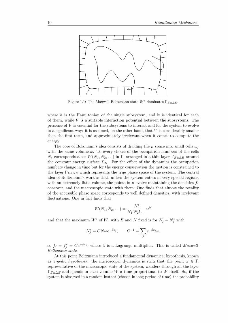
Figure 1.1: The Maxwell-Boltzmann state W ∗ dominates ΓE±∆E .

where h is the Hamiltonian of the single subsystem, and it is identical for eachof them, while V is a suitable interaction potential between the subsystems. Thepresence of V is essential for the subsystems to interact and for the system to evolvein a significant way: it is assumed, on the other hand, that V is considerably smallerthen the first term, and approximately irrelevant when it comes to compute theenergy.

The core of Bolzmann’s idea consists of dividing the µ space into small cells ωjwith the same volume ω. To every choice of the occupation numbers of the cellsNj corresponds a set W (N1, N2, . . .) in Γ, arranged in a thin layer ΓE±∆E aroundthe constant energy surface ΣE . For the effect of the dynamics the occupationnumbers change in time but for the energy conservation the motion is constrained tothe layer ΓE±∆E which represents the true phase space of the system. The centralidea of Boltzmann’s work is that, unless the system enters in very special regions,with an extremely little volume, the points in µ evolve maintaining the densities fjconstant, and the macroscopic state with them. One finds that almost the totalityof the accessible phase space corresponds to well defined densities, with irrelevantfluctuations. One in fact finds that

W (N1, N2, . . .) =N !

N1!N2! . . .ωN

and that the maximum W ∗ of W , with E and N fixed is for Nj = N∗j with

N∗j = CNωe−βεj , C−1 =∑j

e−βεjω,

so fj = f∗j = Ce−βεj , where β is a Lagrange multiplier. This is called Maxwell-Boltzmann state.

At this point Boltzmann introduced a fundamental dynamical hypothesis, knownas ergodic hypothesis: the microscopic dynamics is such that the point x ∈ Γ,representative of the microscopic state of the system, wanders through all the layerΓE±∆E and spends in each volume W a time proportional to W itself. So, if thesystem is observed in a random instant (chosen in long period of time) the probability


of finding the system in a generic set coincides with its volumeW . This interpretationof volume in the phase space as a probability a priori of a set of microscopic statesis commonly called principle of equiprobability of the microscopic states, on whichthe whole statistical mechanics is built: the ergodic hypothesis represents a possibledynamic justification of it.

Boltzmann’s conclusion is that no matter how the system is prepared, evenin condition which are far from the thermodynamic equilibrium, the microscopicdynamics will push the system into W ∗, and in this set it will spend the majority ofits time, up to extremely rare fluctuations.

Gibbs’s notion of macroscopic state is different from the one of Boltzmann’s, theprobability playing a more essential role. While Boltzmann thinks at the µ space,and associates the macroscopic state to a distribution f of the subsystems in the µspace where each of them is defined, Gibbs works directly in Γ, and identifies themacroscopic state as a probability distribution ρ in this space; the interpretation ofρ is that for a generic W ⊂ Γ the a priori probability that one of the microscopicstates x ∈W is realized is

P (W ) =

∫Wρ dV,

where dV is the volume in Γ. Every macroscopic state is then a measure in Γ,with density ρ. Gibbs then considers at each time a family or ensemble of systemsin evolution, independent mental replicas of the same physical system in differentmicroscopic states, distributed in Γ with a suitable probability density ρ. The idea isthat in every experiment the preparation of the system at t = 0 determines a initialdistribution ρ0 in Γ; under the dynamics each initial condition evolves independently,determining at each instant a suitable distribution ρt. From the volume conservationin the phase space follows the evolution equation for ρt

ρt(x) = ρ0(φ−t(x)), x ∈ Γ,

denoting with x 7→ φt(x) the microscopic evolution. The search for equilibrium states,the ones in which ρt(x) in each point x does not depend on t, becomes natural. Anexample of equilibrium distribution is obtained for each ΓE±∆E as

ρ∗(x) =

const in ΓE±∆E

0 elsewhere.

The situation of equiprobability of the microscopic states is then, in Gibbs’s view,an equilibrium state. It is clear that such a state is not unique: in fact, every

ρ∗(x) = F (H(x)),

where F : R → R∗ is arbitrary and H is the Hamiltonian, is an equilibrium state.Indeed, the dynamics preserves the energy, so one must work in a constant energysurface ΣE instead of the whole phase space Γ. One finds that the volume conservationin the phase space induces a conserved measure µ on each constant energy surfaceΣE . At this point one can introduce, instead of the density ρ in Γ, a superficial


density in ΣE , which we keep on calling ρ, and attribute to each set A ⊂ ΣE theprobability

P (A) =

∫Aρ(x)dµ

with the same evolution equation.Our aim is now to give the idea of a dynamical justification of these statistical

assumptions. We will just enter the problem, giving the most basilar definitions andresults, avoiding every kind of technical details.

Definition 1.9. For every function f : M → R, the function f : M → R defined by

f(x) := limt→∞

1

t

t−1∑s=0

f(φs(x))

or in the continuous case

f(x) := limt→∞

1

t

∫ t

0f(φs(x)) ds

is called, if it exists, the time average of f .

For example, the average time of visit of an orbit in a measurable set A

τA(x) := limt→∞

1

tτA(x, t), τA(x, t) :=

∫ t

0χA(φs(x)) ds,

where χA is the characteristic function of A, is precisely the time average of χA. Thetime average of a function f , is itself a function f ; it is instead a number the phaseaverage 〈f〉 of f , defined for every f ∈ L1(M,µ), by

〈f〉 :=

∫Mf dµ.

Theorem 1.1 (Ergodic theorem of Birkhoff-Kinchin). Let (M,µ, φ) a discrete dy-namical system, and be f : M → R in L1. Then the limit

f(x) = limt→∞

1

t

t−1∑s=0

f(φs(x)),

exists almost everywhere in M , and one has

f(φ(x)) = f(x), 〈f〉 = 〈f〉.

If the system is invertible, then the limit

f−(x) = limt→∞

1

t

t−1∑s=0

f(φ−s(x))

exists almost everywhere, and almost everywhere coincides with f

Definition 1.10 (Ergodic system). The dynamical system (M,µ, φ) is said ergodicif one of the following equivalent properties is satisfied:


1. For every summable function f : M → R, time average and phase averagecoincide:

f(x) = 〈f〉 almost everywhere in M ;

2. For every measurable set A ⊂ M the average time of visit is equal to themeasure of A:

τA(x) = µ(A) almost everywhere in M ;

3. There are no summable non-trivial integrals of motion:

f(φt(x)) = f(x) ∀t almost everywhere in M =⇒ f constant in M

for every f : M → R.

The first property is the most classical one, and is at the basis of the definitionof ergodicity in different textbooks of statistical mechanics; it corresponds to thepractical idea of substituting phase averages to time averages, which are in generaldifficult to compute. The second property formalize to the idea by Boltzmann thatin an observation made in a casual time corresponds a probability of finding themicroscopic state of the system in A equal to the measure of A: in this way, for anergodic system, the volume assumes the meaning of probability. The third property,finally, corresponds to the uniqueness of the equilibrium in Gibbs’s sense: if themacroscopic state ρt evolves with

ρt(x) = ρt(φ−t(x))

then the only equilibrium state, such that ρt = ρ0 for every t is the uniform oneρ(x) = 1 almost everywhere.

Clearly, every Hamiltonian system with one degree of freedom, on a constantsurface energy ΣE compact connected and with no singular point, is ergodic. It isergodic, then, the single harmonic oscillator H(q, p) = 1

2(p2 + ω2q2) on each of theconstant energy curves. It is not ergodic instead, on the constant energy surface,a system of two or more harmonic oscillators, H = 1

2

∑ni=1(p2

i + ω2i q

2i ), or more

generally a system like

H(q, p) =n∑i=1

hi(qi, pi);

in fact, the energies of the single components are first integrals, thus going against thethird property. An integrable system with n ≥ 2 degrees of freedom is not ergodic,since it admits n non-trivial first integrals. Systems like these prompt us to put avery natural question: what happens if one includes a small coupling between theoscillators? This is exactly the question to which Fermi, Pasta and Ulam tried toanswer in the celebrated work [1], that is the starting point of this work.


CHAPTER 2

Infinite dimensional systems

Let L2(Λ) be the space of real-valued square integrable function on a one dimen-sional differentiable manifold Λ with norm

〈f, g〉 =

∫Λdx f(x)g(x) ∀f, g ∈ L2(Λ).

In the following we will denote partial derivatives with a subscript, for example∂ψ∂t = ψt.

We would like to give an Hamiltonian structure to an infinite dimensional system,namely a PDE system in the form

ψt = f(ψ,ψx, ψxx, . . .), ψ ∈ L2(Λ).

In this work, in fact, we will use the Heisenberg picture of Quantum Mechanics andits Hamiltonian properties in order to understand the dynamics of the particularquantum system which is the quantum equivalent of the classical Fermi-Pasta-Ulamsystem [1]. With the tools provided by this theory of infinite dimensional systemswe will formulate Quantum Mechanics in an Hamiltonian environment, providing anHamiltonian formulation for the Schrödinger picture, and seeing its isomorphism (inthe algebraic sense) with the Heisenberg picture. Thanks to the Poisson structureof Quantum Mechanics we will in fact extend the theorems known in the classicalenvironment and perform calculations that allows us to keep in close contact to thewell studied classical case.

2.1 Lagrangian formulation

We will introduce the Hamiltonian structure of an infinite dimensional systemstarting by the Lagrangian formulation, and then pass to the Hamiltonian formulationperforming the Legendre transform. In analogy with the finite dimensional case, theLagrangian will be a real functional L(ψ,ψt). Instead of the sum over the discreteindices in the finite dimensional case, we have now a integral over Λ of a function

15

16 Infinite dimensional systems

L (ψ,ψx, ψt) called Lagrangian density

L(ψ,ψt) =

∫Λ

L (ψ,ψx, ψt) dx.

The action is the integral over the time of this quantity

S(ψ) =

∫RL(ψ,ψt) dt =

∫R

∫Λ

L (ψ,ψx, ψt) dx dt

We would like to apply the principle of least action, i.e. find the equations of motionby searching the critical points of the action functional S, but to perform such taskwe need first of all to define differentiation in the infinite dimensional space L2. Inthe finite dimensional case, for a function f : Rn → R, x 7→ f(x) we have

df(x) =d

dεf(x+ εh)|ε=0 = ∇f(x) · h.

In the infinite dimensional case we define the weak differential of a functionalF (ψ1, . . . , ψn) along the direction (h1, . . . , hn), with hi|∂Λ = 0 ∀i = 1, . . . , n

dF (ψ1, . . . ψn) =d

dεF (ψ1 + εh1, . . . , ψn + εhn)|ε=0

and the L2-gradients ∇ψiF such that

dF =

n∑i=1

〈∇ψiF, hi〉.

We now calculate the L2-gradients of L along the directions h, ht

dL(ψ.ψt) =

∫Λ

d

dεL (ψ + εh, ψx + εhx, ψt + εht)|ε=0 dx

=

∫Λ

(∂L

∂ψh+

∂L

∂ψxhx +

∂L

∂ψtht) dx

=

∫Λ

((∂L

∂ψ− d

dx

∂L

∂ψx)h+

∂L

∂ψtht

)dx

so thatdL = 〈∂L

∂ψ− d

dx

∂L

∂ψx, h〉+ 〈∂L

∂ψt, ht〉.

The L2-gradients of L are then

∇ψL =∂L

∂ψ− d

dx

∂L

∂ψx, ∇ψtL =

∂L

∂ψt.

The principle of least action reads dS(ψ) = 0, so

dS(ψ) =

∫RdL(ψ,ψt) dt

=

∫R(〈∇ψL, h〉+ 〈∇ψtL, ht〉) dt

=

∫R

∫Λ

(∇ψL−d

dt∇ψtL)h dx dt

≡ 〈∇ψS, h〉.

Hamiltonian formulation 17

The equation of motion are then

∇ψS = ∇ψL−d

dt∇ψtL = 0 =⇒ ∂L

∂ψ− d

dx

∂L

∂ψx− d

dt

∂L

∂ψt= 0

which are the Euler-Lagrange equations for the Lagrangian density L .

Remark 2.1. In theoretical physics a slightly different notation is used, which we willuse in the following. The weak differential

dF (ψ) := δF (ψ)

is called Gateaux differential while h =: δψ so that

δF (ψ) =d

dεF (ψ + εδψ)|ε=0.

The L2-gradient are called functional derivative ∇ψF =: δFδψ so that

δF (ψ) = 〈δFδψ

, δψ〉.

The Euler-Lagrange equation thus reads

d

dt

δL

δψt− δL

δψ= 0. (2.1)

2.2 Hamiltonian formulation

In analogy to the well known finite dimensional case, we define the momentum

π =δL

δψt.

Suppose the above relation is invertible, i.e. it exists a smooth function F such that

ψt = F (ψ, π).

This hypothesis is verified, for example, if L is convex in ψt, but it is not if thedependence is linear. Starting from a Lagrangian functional L we can now define theHamiltonian as its Legendre transform

H(ψ, π) = (〈π, ψt〉 − L(ψ,ψt)) |ψt=F (ψ,π)

which can be written as a function of a Hamiltonian density H as H =∫

Λ H dxwhere

H = (πψt −L (ψ,ψx, ψt))|ψt=F (ψ,π).

In the following we will understand the evaluation of ψt in F (ψ, π). The actionfunctional is S(ψ, π) =

∫(〈π, ψt〉 −H(ψ, π)) dt. A direct computation shows that

the least action principle implies the Hamilton equations for ψ and π, i.e.

ψt =δH

δπ, πt = −δH

δψ.


In this way we have seen that ψ and π defined as above are a infinite dimensionalHamiltonian system, with the standard Poisson tensor J and the standard partialderivative substituted by functional derivatives(

ψtπt

)= J

( δHδψδHδπ

).

Moreover, the algebra of real-valued, square-integrable functions of ψ and π togetherwith the Poisson tensor J form a Poisson algebra, which can be object of changes ofvariables and canonical transformations as described in the previous section.

2.3 Quantum mechanics

2.3.1 Hamiltonian structure of the Schrödinger equation

Let us consider the Schrödinger equation for the wave function ψ : Λ× R→ C,x 7→ ψ(x, t), of a single particle with massm > 0 and position x in some d-dimensionaldifferentiable manifold1 Λ in a potential V (x)

i~∂ψ

∂t= Hψ = − ~2

2m∆ψ + V ψ. (2.2)

Our aim is to look for an Hamiltonian formulation of this equation, i.e. look foran Hamiltonian, function of ψ(x, t), whose Hamilton equations are precisely theSchrödinger equation (and its complex conjugate). Of course this whole constructioncan be extended to the many-particle case.

First of all we want to formulate the problem in a Lagrangian environment. TheSchrödinger equation and its complex conjugate are the Euler-Lagrange equationsfor the Lagrangian density

L (ψ,ψ∗, ψt, ψ∗t ) =

i~2

(ψ∗ψt − ψψ∗t )− V |ψ|2 − ~2

2m|∇ψ|2 (2.3)

and L =∫

Λ L dx. In fact, the Euler-Lagrange equation for ψ∗ are

d

dt

δL

δψ∗t=

δL

δψ∗=⇒ d

dt(−i~ψ) = −V ψ −

d∑j=1

d

dxj(− ~2

2m

∂ψ

∂xj)

which is of course (2.2). One would like to apply the Legendre transform in order topass to the Hamiltonian formulation, but as L is linear in ψt and ψ∗t , the change ofvariables

π =δL

δψt

is not invertible, and the whole construction of the Legendre transform theory cannotbe applied. However, if we define ψ as the "coordinate" and i~ψ∗ as the "momentum"and use the standard Poisson tensor J2, we have a Hamiltonian system of Hamiltonian

H =

∫Λ

H dx, H =~2

2m|∇ψ|2 + V |ψ|2.

1Common choices for Λ are Rd, or the torus Td ≡ (R/lZ)d for some l > 0, for d = 1, 2, 3.

Quantum mechanics 19

In fact, the Hamilton equations are

ψt =δH

δπ=

1

i~δH

δψ∗=

1

i~(∂H

∂ψ∗−∇ · ~

2

2m

∂|∇ψ|2

∂∇ψ∗) =

1

i~(− ~2

2m∆ψ + V ψ)

which is (2.2), and

πt = i~ψ∗t = −δHδψ

which gives its complex conjugate. One can also use the so called Birkhoff structure,which is a more symmetric Poisson structure where ψ is the coordinate and ψ∗ isthe momentum. In these coordinates, the Poisson tensor is σ2

~ , in fact the Hamiltonequations are (

ψtψ∗t

)=

1

~

(−i δHδψ∗i δHδψ

)=

1

i~J2

(δHδψδHδψ∗

)and 1

iJ2 = σ2. Observe that, in this Poisson algebra, the Poisson bracket of twofunctions F (ψ,ψ∗) and G(ψ,ψ∗) is given by

F,G =1

i~

∫Λ

(δF

δψ

δG

δψ∗− δF

δψ∗δG

δψ) dx.

Remark 2.2. The Hamiltonian H(ψ,ψ∗), namely

H(ψ,ψ∗) =

∫Λ

(~2

2m|∇ψ|2 + V |ψ|2) dx =

∫Λψ∗Hψ dx = 〈ψ, Hψ〉

is the quadratic (Hermitian) form associated to H (the Hamiltonian operator)computed in ψ.

2.3.2 Schrödinger and Heisenberg pictures as Poisson algebras

We have just shown that the Schrödinger equation admits a Hamiltonian formu-lation in terms of the Poisson bracket

F,G =1

i~

∫Λ

(δF

δψ

δG

δψ∗− δF

δψ∗δG

δψ) dx

with Hamiltonian H(ψ,ψ∗) = 〈ψ, Hψ〉. Here the phase space of the system isthe space L2 of complex valued, square-integrable wave-functions, and the PoissonAlgebra is the algebra of real functions F (ψ,ψ∗) endowed with the bracket , defined above. In this picture, called Schrödinger picture, the wave function evolvesin time, and the functions defined on the phase space evolve as a consequence.

ψ(0) −→ ψ(t)↓ ↓

F (ψ(0), ψ∗(0)) −→ F (ψ(t), ψ∗(t))

An alternative formulation of quantum mechanics is the following. First, the flowof the Schrödinger equation is explicitly introduced, in the form of a unitary time-evolution operator U(t) solution of

i~d

dtU(t) = HU(t), U(0) = 1.


One easily checks that, due to the above equation and initial condition, U †(t)U(t) = 1

∀t ∈ R. For the sake of simplicity H and all the other self-adjoint operators aresupposed to be independent of time. One then finds

U(t) = e−i~ Ht :=

∑j≥0

1

j!(− i

~Ht)j .

Second, it is postulated that the relevant physical quantities that are measurable, i.e.the so-called observables, correspond to the quadratic (Hermitian) forms associatedto certain self-adjoint linear operatos, computed in ψ(t), namely

〈ψ(t), Aψ(t)〉, where A† = A.

The above quadratic form is called the quantum expectation of the operator A attime t. Now, one has

〈ψ(t), Aψ(t)〉 = 〈ψ(0), AH(t)ψ(0)〉

where AH(t) := U †(t)AU(t). In other words, the quantum expectation of thetime-independent operator A a time t equals the quantum expectation of the timedependent operator AH(t) at time t = 0. One can thus think of the wave function asfixed to its initial value, letting the operators evolve in time. This is the so-calledHeisenberg picture. In such a picture the operators evolve according to the similaritytransformation A→ U †(t)AU(t) =: AH(t). One easily finds that

d

dtAH(t) =

1

i~[AH(t), H(t)]

called the Heisenberg equation of motion for AH(t). Observe that the bracket 1i~ [ , ]

is a bilinear, skew-symmetric, Jacobi and Leibniz product in the space of self-adjointoperators: a Poisson bracket on the algebra of linear self-adjoint operatos acting onL2, which then becomes a Poisson algebra.

In order to compare the Poisson algebra of the Schrödinger picture to that ofthe Heisenberg picture, one has to restrict the algebra of the functions in the formerpictures to that of the real quadratic functions. Thus, to any such function F (φ, φ∗)there correspond a linear self-adjoint operator F such that F (ψ,ψ∗) = 〈ψ, Fψ〉,and such a correspondence is a bijection. Now, given F (ψ,ψ∗) = 〈ψ, Fψ〉 andG (ψ,ψ∗) = 〈ψ, Gψ〉, one has

F ,G =1

i~

∫Λ

(δF

δψ

δG

δψ∗− δF

δψ∗δG

δψ) dx

=1

i~

∫Λ

[(Fψ∗)Gψ − (Fψ)Gψ∗] dx

=1

i~[〈ψ, F Gψ〉 − 〈ψ, GFψ〉]

= 〈ψ, 1

i~[F , G]ψ〉

i.e.〈ψ, Fψ〉, 〈ψ, Fψ〉 = 〈ψ, 1

i~[F , G]ψ〉.

Quantum mechanics 21

Such a relation shows that the Poisson algebras of the Schrödinger and of theHeisenberg picture are isomorphic. More precisely, the map

Q : F 7→ F = Q(F ) := 〈ψ, Fψ〉

that associates linear self-adjoint operators to their quadratic forms, (elements ofthe Heisenberg algebra to elements of the Schrödinger algebra) is a bijection andpreserves the product

Q(F ), Q(G) = Q(1

i~[F , G]).

Thus Q is a isomorphism between the two algebras.


CHAPTER 3

The classical FPU problem and its quantization

After World War II, Fermi became interested in the development and potentialitiesof the electronic computing machines, trying a selection of problems for heuristicwork where in absence of closed analytic solutions experimental work on a computingmachine would perhaps contribute to the understanding of properties of solutions, forexample regarding long-time behaviour of non-linear physical systems. In particular,the first of these work was the study of the ergodic properties of a one-dimensionalanharmonic chain, which was the simplest non-linear model for a metal, expectingthe thermalisation to show. In particular:

– A chain of 64 particles with fixed boundary conditions was considered, theforce between the particles satisfying the Hooke Law, plus weak non-linearcorrections;

– The equations of motion were resolved numerically;

– The results were analysed in Fourier components and plotted against time.

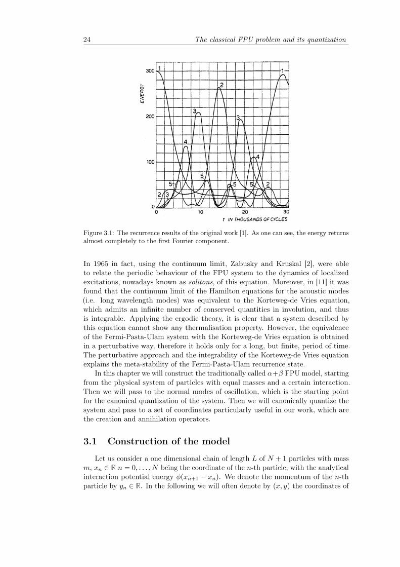
The initial data were chosen by setting all the energy in the first Fourier componentand the program was let run, waiting for an energy equipartition state, in which allthe Fourier components had approximately the same amount of energy.

The results, shown in figure 3.1 were quite surprising, and became known asthe Fermi-Pasta-Ulam paradox : instead of the energy equipartition, a recurrentmeta-state was found in which the energy is exchanged by the lower Fourier modesonly, and after some time the system recurs to the initial data, the ∼ 97% of theenergy returning to the first Fourier component. These results were one of the firstintimations that the prevalent (at those times) beliefs in the universality of mixingand thermalisation in non-linear systems may not be always justified.

The solution of the paradox can be seen in multiple equivalent ways, one of thembeing the existence and stability of solitons for the Korteweg-de Vries equation

Ut = aUxxx + bUUx.

23

24 The classical FPU problem and its quantization

Figure 3.1: The recurrence results of the original work [1]. As one can see, the energy returnsalmost completely to the first Fourier component.

In 1965 in fact, using the continuum limit, Zabusky and Kruskal [2], were ableto relate the periodic behaviour of the FPU system to the dynamics of localizedexcitations, nowadays known as solitons, of this equation. Moreover, in [11] it wasfound that the continuum limit of the Hamilton equations for the acoustic modes(i.e. long wavelength modes) was equivalent to the Korteweg-de Vries equation,which admits an infinite number of conserved quantities in involution, and thusis integrable. Applying the ergodic theory, it is clear that a system described bythis equation cannot show any thermalisation property. However, the equivalenceof the Fermi-Pasta-Ulam system with the Korteweg-de Vries equation is obtainedin a perturbative way, therefore it holds only for a long, but finite, period of time.The perturbative approach and the integrability of the Korteweg-de Vries equationexplains the meta-stability of the Fermi-Pasta-Ulam recurrence state.

In this chapter we will construct the traditionally called α+β FPU model, startingfrom the physical system of particles with equal masses and a certain interaction.Then we will pass to the normal modes of oscillation, which is the starting pointfor the canonical quantization of the system. Then we will canonically quantize thesystem and pass to a set of coordinates particularly useful in our work, which arethe creation and annihilation operators.

3.1 Construction of the model

Let us consider a one dimensional chain of length L of N + 1 particles with massm, xn ∈ R n = 0, . . . , N being the coordinate of the n-th particle, with the analyticalinteraction potential energy φ(xn+1 − xn). We denote the momentum of the n-thparticle by yn ∈ R. In the following we will often denote by (x, y) the coordinates of

Construction of the model 25

the whole phase space. Here we will consider fixed boundary conditions, i.e.

x0 = 0, xN = L, y0 = 0, yN = 0. (3.1)

The Hamiltonian of the system will then be

K =

N−1∑n=1

y2n

2m+

N−1∑n=0

φ(xn+1 − xn). (3.2)

Since the Hamilton equations are

yk = − ∂K∂xk

= φ′(xk+1 − xk)− φ′(xk − xk−1)

xk =∂K

∂yk=ykm,

the system surely has (at least) the equilibrium (xeq, yeq) such that

yeqn = 0, xeqn+1 − xeqn = xeqn − x

eqn−1 ∀n. (3.3)

This physically corresponds to a state where all the particles stay still and equallydistant from one another. Denoting with a the interspacing between the particles inthe equilibrium configuration one has

xeq0 = 0, xeq1 = a, xeq2 = 2a, . . . , xeqn = na, . . . , xeqN = Na,

so, given the boundary conditions, surely Na = L, which is the classic crystalconfiguration.

Now we want to change coordinates, putting us in a frame where only smalldeviations from the equilibrium are considered. Moreover, we want to deal onlywith non dimensional quantities. With this in mind we will operate the change ofcoordinates (xn, yn) 7→ (qn, pn) and the reparametrization of the time T 7→ t thatconjugates K to H, where

xn = na+ aqn, yn = maτ pn

T = τt, K = ma2

τ2 H.(3.4)

Remark that we denoted with T the old dimensional time, t the new non dimensionaltime, and τ ∈ R a parameter yet to be specified. With the rescaling of the Hamiltonianand the time, this transformation is canonical. The boundary conditions 3.1 become

q0 = p0 = qN = pN = 0. (3.5)

With this new coordinates the Hamiltonian K 3.2 becomes (yet to be rescaledaccording to 3.4)

K =

N−1∑n=1

ma2

τ

p2n

2+N−1∑n=0

φ(a+ a(qn+1 − qn)).


In the same frame of mind, denoting δnq := qn+1 − qn, and being the interactionpotential energy analytic, we can expand it in Taylor expansion around the point a,obtaining

φ(a+ aδnq) =∑s≥0

φ(s)(a)

s!as(δnq)

s.

The potential energy will be

∑s≥0

φ(s)(a)

s!as

N−1∑n=0

(δnq)s =

φ(a)N + φ′(a)N−1∑n=0

(qn+1 − qn) +∑s≥2

φ(s)(a)

s!as

N−1∑n=0

(qn+1 − qn)s.

Being∑N−1

n=0 (qn+1 − qn) = 0 (it is easy to verify keeping in mind the fixedboundary conditions), and eliminating the constant term, one can write the potentialenergy

φ(2)(a)a2

2

N−1∑n=0

(qn+1 − qn)2 +φ(3)(a)a3

3!

N−1∑n=0

(qn+1 − qn)3+

+φ(4)(a)a4

4!

N−1∑n=0

(qn+1 − qn)4 + . . .

Remark that by assuming that the equilibrium is stable, one must require thatφ(2)(a) > 0.

The new Hamiltonian is

H =

N−1∑n=1

p2n

2+∑s≥2

φ(s)(a)as−2τ2

ms!

N−1∑n=0

(qn+1 − qn)s, (3.6)

still containing the arbitrary parameter τ , which will be chosen by setting thecoefficient of the quadratic term of the Taylor expansion τ2 φ

(2)(a)m = 1, that is

τ =

√m

φ(2)(a).

With this choice of τ , the following coefficients are

α :=φ(3)(a)a

2φ(2)(a),

β :=φ(4)(a)a2

6φ(2)(a),

γ :=φ(5)(a)a3

24φ(2)(a), . . .

so that the Hamiltonian has the traditional form of the Fermi-Pasta-Ulam Model(also known as FPU )

H =

N−1∑n=1

p2n

2+N−1∑n=0

[1

2(qn+1 − qn)2 +

α

3(qn+1 − qn)3 +

β

4(qn+1 − qn)4 + . . .

]. (3.7)

Construction of the model 27

Remark 3.1. The non-dimensional parameters τ , α, β, ecc. . . are obtainable from thephysical potential φ, the number of particles N and the length of the chain L. Someexamples of these parameters for various potentials are found in [20].

Remark 3.2. If α 6= 0 one can set α = 1, by means of the canonical transformationqn 7→ q′n and a reparametrization of the time t 7→ t′ that conjugates H to H ′ suchthat

qn =q′nα, pn =

p′nα

t = t′, H =H ′

α2,

and then redefining β′ = β/α2, γ′ = γ/α3, . . .

Remark 3.3. Here we use fixed boundary conditions, which are a particular caseof the periodic ones, in the following sense. Given a FPU system with M = 2Nparticles with periodic boundary conditions, i.e.

qj+M = qj , pj+M = pj ∀j,

one can find a particular set of initial data whose evolution is precisely the evolutionof a FPU system with N particles and fixed boundary conditions. In fact, supposethat the Hamiltonian for 2N particle with periodic boundary condition is

H(q, p) =N−1∑

n=−N+1

p2n

2+

N−1∑n=−N+1

u(qm+1 − qn)

and suppose we take a set of initial data which satisfy to the condition

qn = −q−n, pn = −p−n, ∀n.

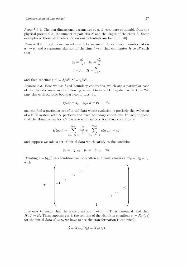
Denoting z = (q, p) this condition can be written in a matrix form as Tz0 =: z′0 = z0,with

T : =

−1. . .

−1. . .

−1−1

. . .−1

. . .−1

It is easy to verify that the transformation z 7→ z′ = Tz is canonical, and thatH T = H. Thus, supposing zt is the solution of the Hamilton equations zt = XH(z0)for the initial data z′0 = z0 we have (since the transformation is canonical)

z′t = XHT (z′0) = XH(z0).


So Tzt and zt are solutions of the same differential equation with the same initialdata, and for the Cauchy–Lipschitz theorem they are the same solution, zt = Tzt.Physically, for such initial data the dynamics maintain the condition

qn = −q−n, pn = −p−n, ∀n

true: the motion is then symmetric, the coordinates with positive n mirroring theones with negative n, while (q0, p0) = (qN , pN ) = 0. It is exactly the dynamics of aN particle system with fixed boundary condition.

3.2 Normal modes

From now on we shall consider only FPU models (3.7) truncated up the 4-thorder, called α+ β models. Let us now introduce the normal modes of oscillation ofthe FPU chain, i.e. a canonical transformation

N : (q, p)n 7→ (Q,P )k (3.8)

such that, defining φk(n) :=√

2N sin πkn

N , one has

N :

Qk =

∑N−1n=1 qnφk(n)

Pk =∑N−1

n=1 pnφk(n)

and on the other hand

N −1 :

qn =

∑N−1k=1 Qkφk(n)

pn =∑N−1

k=1 Pkφk(n)

Remark 3.4. One has∑N−1

n=1 φk(n)φk′(n) = δk,k′ (see lemma 3.2).

Proposition 3.1. This change of variables conjugates the Hamiltonian 3.7 to theHamiltonian1 H := H N −1

H(Q,P ) =

N−1∑k=1

P 2k + ω2

kQ2k

2+∑D>2

gDD(2N)D/2−1

N−1∑k1,...,kD

∆D(k1, . . . , kD)

D∏s=1

ωksQks

(3.9)where

ωk := 2 sinπk

2N, k = 1, . . . , N − 1

are the frequencies and

∆D(k1, . . . , kD) :=1

2

∑σ∈SD

δσ·k,0 +∑σ∈SD

∑l≥1

(−1)lδσ·k,2lN

are called selectors, where S = −1, 1 .

Now we show how we got to (3.9).1In order to avoid heavy notations, we will use the same symbol for conjugated Hamiltonians.

Normal modes 29

Lemma 3.1.∑N−1

n=0 cos πknN =∑

s∈Z(Nδk,2sN + δk,2s+1)

Proof. Let us begin by calculating the quantity∑N−1

n=0 eiπknN (the result will be its

real part). Note that if k ∈ 2ZN then the result is simply N .N−1∑n=0

eiπknN =

1− eiπk

1− eiπkN

=eiπk − 1

eiπk2N (ei

πk2N − e−i

πk2N )

=e−i

πk2N ((−1)k − 1)

2i sin πk2N

.

Now we take the real part:

ReN−1∑n=1

eiπknN = Re

(e−i

πk2N ((−1)k − 1)

2i sin πk2N

)=

1

2(1− (−1)k) =

0 if k is even1 if k is odd

Lemma 3.2.∑N−1

n=1 φn(k)φn(k′) = δk,k′

Proof. Using the prosthaphaeresis formula sinα sinβ = 12(cos (α− β)− cos (α+ β)),

one finds thatN−1∑n=1

φn(k)φn(k′) =1

N

N−1∑n=1

(cosπ(k − k′)n

N− cos

π(k + k′)n

N).

Now we use Lemma 3.1 and find1

2

∑s∈Z

[N(δk−k′,2sN − δk+k′,2sN ) + (δk−k′,2s+1 − δk+k′,2s+1)].

Now, 1 ≤ k, k′ ≤ N − 1, so 2 ≤ k + k′ ≤ 2N − 2 and 2−N ≤ k − k′ ≤ N − 2: thefirst term is non zero only if k − k′ = 0; besides, if k + k′ is odd k − k′ is also odd:the second term is always zero. The result is then 1

NNδk−k′,0 = δk,k′ .

By using Lemma 3.2 one can easily see that the kinetic part of (3.7) becomesN−1∑n=1

p2n

2|pn=

∑N−1k=1 Pkφk(n) =

N−1∑k=1

P 2k

2.

Now we will show how to compute the perturbation part, i.e.N−1∑n=0

U(qn+1 − qn)|qn=∑N−1k=1 Qkφk(n),

whereU(x) =

∑D≥2

gDDxD.

Note that g2 = 1, g3 = α, g4 = β and so on. First of all let us compute the differenceqn+1 − qn for a generic n = 0, . . . , N − 1. One has

qn+1 − qn =

N−1∑k=1

Qk(φn+1(k)− φn(k))

=N−1∑k=1

Qk

√2

N(sin

πk(n+ 1)

N− sin

πkn

N)

=

N−1∑k=1

ωkQk

√2

Ncos

πk(2n+ 1)

2N.


So, the D-degree perturbation energy will be

gDD

N−1∑n=0

(qn+1 − qn)D =gDD

(2

N

)D/2 N−1∑k1,...,kD=1

D∏s=1

ωksQks

N−1∑n=0

D∏s=1

cosπks(2n+ 1)

2N.

In order to do this computation, a general formula for the product of cosines will beuseful.

Lemma 3.3. ∀D ∈ N, let be θ(D) = (θ1, . . . , θD) and S = −1, 1. Then,D∏s=1

cos θs =1

2D

∑σ∈SD

cos (σ · θ(D)).

Proof. We will proceed by induction. The formula is trivially true for D = 1. Supposeit is true for a generic D. Then,

D+1∏s=1

cos θs =1

2D

∑σ∈SD

cos (σ · θ(D)) cos θD+1

=1

2D+1

∑σ∈SD

[cos (σ · θ(D) + θD+1) + cos (σ · θ(D) − θD+1)

=1

2D+1

∑σ∈SD+1

cos (σ · θ(D+1))

Using Lemma 3.3 the D-degree perturbation energy becomes

gDD

N−1∑n=0

(qn+1 − qn)D =

gDD

(2

N

)D/2 1

2D

N−1∑k1,...,kD=1

D∏s=1

ωksQks

N−1∑n=0

∑σ∈SD

cos

(π(2n+ 1)

2Nk · σ

),

where k = (k1, . . . , kD).

Lemma 3.4. If k ∈ Z one hasN−1∑n=0

cosπk(2n+ 1)

2N=∑s∈Z

(−1)sNδk,2sN .

Proof. First of all we compute∑N−1

n=0 eiπk(2n+1)

2N , and the result will be its real part.One can see that, if k = 2sN , s ∈ Z, then the result is (−1)sN . Otherwise one has

N−1∑n=0

eiπk(2n+1)

2N = eiπk2N

N−1∑n=0

eiπknN

= eiπk2Ne−i

πk2N ((−1)k − 1)

2i sin ( πk2N )

=i

2

1− (−1)k

sin ( πk2N ).

So in this case Re(∑N−1

n=0 eiπk(2n+1)

2N ) = 0.

Normal modes 31

Let us now define the selector

∆D(k1, . . . , kD) :=1

2

∑σ∈SD

∑l∈Z

(−1)lδσ·k,2lN . (3.10)

An alternative but completely equivalent form of the selector is

∆D(k1, . . . , kD) =1

2

∑σ∈SD

δσ·k,0 +∑σ∈SD

∑l≥1

(−1)lδσ·k,2lN . (3.11)

By means of this definition and of Lemma 3.4 one can see that the D-degreeperturbation energy can be written in a more compact way[

gDD

(2

N

)D/2 N

2D−1

]N−1∑

k1,...,kD=1

∆D(k1, . . . , kD)

D∏s=1

ωksQks (3.12)

For example, let us write the selectors of degree two, three, and four. For D = 2

∆2(k1, k2) = δk1,k2 .

For D = 3

∆3(k1, k2, k3) = δk1+k2,k3 + δk2+k3,k1 + δk3+k1,k2 − δk1+k2+k3,2N . (3.13)

For D = 4,

∆4(k1, k2, k3, k4) = δk1+k2+k3,k4 + δk2+k3+k4,k1 + δk3+k4+k1,k2 + δk4+k1+k2,k3+

+ δk1+k2,k3+k4 + δk1+k3,k2+k4 + δk1+k4,k2+k3+

− δk1+k2+k3,k4+2N − δk1+k2+k4,k3+2N − δk1+k3+k4,k2+2N+

− δk2+k3+k4,k1+2N − δk1+k2+k3+k4,2N .

(3.14)

In this way, one can compute explicitly the Hamiltonian (3.9), and find

H =N−1∑k=1

P 2k + ω2

kQ2k

2+∑D=3,4

gD

D(2N)D/2−1

N−1∑k1,...,kD

∆D(k1, . . . , kD)D∏s=1

ωksQks

Remark 3.5. H2 =∑N−1

k=1P 2k+ω2

kQ2k

2 is precisely the Hamiltonian of N −1 non coupledharmonic oscillators, so, in a sense, is integrable. Thus here we are considering N − 1coupled oscillators with cubic and quartic interaction.

One can now perform a canonical rescaling, namely a symplectic change ofcoordinates (Q,P ) 7→ (Q′, P ′) such that

Qk =Q′k√ωk, Pk =

√ωkP

′k, k = 1, . . . , N − 1

which conjugates the Hamiltonian (3.9) to

H(Q′, P ′) =N−1∑k=1

ωkP ′2k +Q′2k

2

+∑D≥3

gDD(2N)D/2−1

N−1∑k1,...,kD

∆D(k1, . . . , kD)

D∏s=1

√ωksQ

′ks . (3.15)


In order to perform quantization, it is useful to pass to complex coordinates, i.e.

zk :=Q′k + iP ′k√

2, z∗k :=

Q′k − iP ′k√2

k : 1, . . . , N − 1. (3.16)

This conjugates (3.15) to

H(z, z∗) =N−1∑k=1

ωk|zk|2

+∑D≥3

gDDND/2−12D−1

N−1∑k1,...,kD

∆D(k1, . . . , kD)D∏s=1

√ωks(zks + z∗ks). (3.17)

Remark 3.6. The change of coordinates (3.16) is not symplectic, so it does notpreserve the poisson structure. One can easily see with a direct computation thatthe new Poisson structure is

zk, z∗k′ = −iδk,k′

so that the ODEs related to H are

zk = −i∂H∂z∗k

= −iωkzk + . . .

and its complex conjugate for z∗k.The Hamiltonian (3.17) is the starting point of the analysis in [11], in which

it was found that the Hamilton equations for the first modes zk, k N are, in acertain way that will be specified in the following, equivalent to the Korteweg-deVries equation. Our aim is to quantize this system, and find out which equation isthe quantum equivalent of the KdV, using the tool of the Hamiltonian theory ofperturbations. We will write the calculations for the quantum case, while, since thecomputations are very similar and differ only for the commutativity of products, weonly report the results for the classical case.

3.3 Canonical quantization of the FPU problem

In order to quantize the FPU problem, one can proceed in two different, but aswe will show, completely equivalent ways.

The first is to start from the "physical" Hamiltonian (3.2), rescale the momentaand the positions to obtain non dimensional quantities, and then pass to the normalmodes of oscillation (Q,P ). Finally quantize the momenta, namely substitute Pkand Qk, ∀k = 1, . . . , N − 1, with hermitian non dimensional operators Pk and Qksuch that

Pk = −i ∂

∂Qk∀k.

The second is to start from the "physical" Hamiltonian (3.2) and canonically quantizethe momenta yn and coordinates xn, namely substitute yn, and xn ∀n = 1, . . . , N−1,with hermitian dimensional operators yn and xn such that

yn = −i~ ∂

∂xn∀n.

Canonical quantization of the FPU problem 33

Then, rescale (x, y) in order to obtain non dimensional quantities (q, p) such that

pn = −i ∂∂qn

∀n,

and then pass to the normal modes of oscillation (Q, P ), and find again

Pk = −i ∂

∂Qk∀k.

The first way is the continuation of what we did in the previous sections. Here wewill proceed with the second alternative method, and show its equivalence with thefirst.

Consider a quantum Hamiltonian operator

K =N−1∑n=1

y2n

2m+N−1∑n=0

φ(xn+1 − xn), yn = −i~ ∂

∂xn∀n = 1, N − 1.

This is a Hamiltonian system in the Poisson algebra of the Heisenberg picture, so allthe notions from Hamiltonian mechanics are well defined. We look for a canonicalnon univalent transformation (x, y, K, T ) 7→ (q, p, H, t) of the form

xn = na+ αqn, yn = βpn

K = γH, T = τt

which conjugates K to

H =

N−1∑n=1

p2n

2+

N−1∑n=0

[(qn+1 − qn)2

2+ α

(qn+1 − qn)3

3+ β

(qn+1 − qn)4

4+ . . .

]such that:

1. αβ = γτ ;

2. in order to "normalize" the kinetic energy β2 = γm;

3. in order to "normalize" the quadratic term of the potential energy φ(2)(a)α2 =γ;

4. pn = −i ∂∂qn

.

The last condition is satisfied if and only if

αβ = ~.

We have four equations for four parameters. The solution is

α =

√~

(mφ(2)(a))1/4, β =

√~(mφ(2)(a))1/4, γ = ~

√φ(2)(a)

m, τ =

√m

φ(2)(a).


When passing to the normal modes of oscillationqn =

∑k Qkφk(n)

pn =∑

k Pkφk(n),

Qk =

∑n qnφk(n)

Pk =∑

n pnφk(n),

where φk(n) =√

2N sin (πknN ), the condition Pk = −i ∂

∂Qkis automatically satisfied.

In fact, being∂

∂qn=∑k

∂Qk∂qn

∂

∂Qk=∑k

φk(n)∂

∂Qk,

one has

Pk =∑n

φk(n)(−i ∂∂qn

) =∑n

∑k′

φk(n)φk′(n)(−i ∂

∂Qk′) = −i ∂

∂Qk.

Remark 3.7. It is easy to verify that the operators Qk and Pk satisfy the commutationrule

[Qk, Pk′ ] = iδk,k′ .

We have shown that one can obtain in two different but equivalent ways thequantum Hamiltonian operator for the FPU problem, as a function of the normalmodes of oscillation Qk, Pk, as in 3.9:

H(Q, P ) =N−1∑k=1

P 2k + ω2

kQ2k

2+∑D≤2

gD

D(2N)D/2−1

N−1∑k1,...,kD

∆D(k1, . . . , kD)

D∏s=1

ωksQks .

As we did in the previous section, one can now perform a canonical rescaling, namelya symplectic change of coordinates (Q, P ) 7→ (Q′, P ′) such that

Qk =Q′k√ωk, Pk =

√ωkP

′k, k = 1, . . . , N − 1

which conjugates the previous Hamiltonian to

H(Q′, P ′) =

N−1∑k=1

ωkP ′

2

k + Q′2

k

2

+∑D≥3

gDD(2N)D/2−1

N−1∑k1,...,kD

∆D(k1, . . . , kD)D∏s=1

√ωksQ

′ks . (3.18)

At this point, it is useful to introduce the annihilation and creation operators2 ak anda†k which are the analogous of the complex coordinates introduced in the previouschapter. We define

ak =Q′k + iP ′k√

2, a†k =

Q′k − iP ′k√2

.

2Since the symbols a and a† will be used only to indicate these operators, the circumflex will beomitted.

Normal Ordering 35

They inherit the commutation rule from the one of Q′k and P ′k: being [Q′k, P′q] = iδk,q

one obtains[ak, a

†q] =

δk,q2

+δk,q2

= δk,q

while the other mixed commutators are always zero. This conjugates the Hamiltonianoperator 3.18 to

H(a, a†) =

N−1∑k=1

ωka†kak

+∑D≥3

gDDND/2−12D−1

N−1∑k1,...,kD=1

∆D(k1, . . . , kD)D∏s=1

√ωks(aks + a†ks), (3.19)

and we will call

V (a, a†) =∑D≥3

gDDND/2−12D−1

N−1∑k1,...,kD

∆D(k1, . . . , kD)D∏s=1

√ωks(aks + a†ks)

the perturbation term. We will call in the following the Hamiltonian operator (3.19)the quantum Fermi-Pasta-Ulam (or qFPU ) Hamiltonian. It is important to noticethat we arrived to this formulation of the quantum problem simply starting from thecanonical quantization of the physical Hamiltonian, so the only physical assumptionthat we made is the validity of the canonical quantization, i.e. to substitute to themomentum yn an operator

yn = −i~ ∂

∂xn.

3.4 Normal Ordering

Here we will show the normal ordering of the Hamiltonian of the α+ β model.First of all we need to define it.

Definition 3.1. Given A a product of any number of operators ak and a†k, ∀k, wedefine

– N [A] is the product of the same operators in A rearranged in a way such asall the a† operators are to the left, taking into account the commutation rule[ak, a

†q] = δk,q: N [A] is said the normal ordering of A;

– : A : is the product of the same operators in A rearranged in a way such as allthe a† operators are to the left, without taking into account the commutationrule [ak, a

†q] = δk,q (so treated as if they were commuting real numbers);

Remark 3.8. N [A] and A are the same operator: only its functional form changes.: A : and A instead are two different operators.

So, for example, given A = aka†q

N [A] = a†qak + δk,q, : A : = a†qak.


The normal ordering of

2∏s=1

(aks + a†ks) = ak1ak2 + ak1a†k2

+ a†k1ak2 + a†k1

a†k2.

is more complicated. The first, third and fourth term are already ordered normally,so we just have to rearrange the second term replacing ak1a

†k2

with a†k2ak1 + δk1,k2 .

So one has

:

2∏s=1

(aks + a†ks) : = ak1ak2 + a†k2ak1 + a†k1

ak2 + a†k1a†k2

,

N

[2∏s=1

(aks + a†ks)

]= ak1ak2 + a†k2

ak1 + a†k1ak2 + a†k1

a†k2+ δk1,k2 .

The normal ordering of terms like∏Ds=1(aks + a†ks) grows exponentially with the

degree D, so one can imagine that normal ordering this kind of quantities becomesmore and more complicated.

Our aim is to normal order the qFPU Hamiltonian operator(3.19) for the α+ βmodel, namely

H(a, a†) =N−1∑k=1

ωka†kak

+∑D=3,4

gDDND/2−12D−1

N−1∑k1,...,kD

∆D(k1, . . . , kD)D∏s=1

√ωks(aks + a†ks),

where the aks and a†ks are called respectively annihilation operators and creation

operators, and where we dropped out the constant term∑

kωk2 (which refers to the

vacuum energy). This manipulation of the Hamiltonian operator will be useful whenwe will apply the perturbation theory. The quadratic term is already normal ordered,so we will start by normal ordering the perturbation term. We will denote by H3

and H4 the cubic and quartic term of the Hamiltonian, i.e.

H3(a, a†) =α

12√N

N−1∑k1,k2,k3=1

∆3(k1, k2, k3)3∏s=1

√ωks(aks + a†ks) (3.20)

H4(a, a†) =β

32N

N−1∑k1,k2,k3,k4=1

∆4(k1, k2, k3, k4)4∏s=1

√ωks(aks + a†ks). (3.21)

We will need to compute quantities like

N−1∑k1,...,kD=1

∆D(k1, . . . , kD)N

[D∏s=1


],

where ωk and ∆D are defined in the previous sections, forD = 3, 4, where the productsare made with increasing s (remind that products of operators do not commute) Let

Normal Ordering 37

us forget about the frequencies for the moment (they are real commuting numbers).Let us start to compute

N

[D∏s=1

(aks + a†ks)

].

For D = 3 one has

N

[3∏s=1

(aks + a†ks)

]=

:3∏s=1

(aks + a†ks) : + δk1,k2(ak3 + a†k3) + δk1,k3(ak2 + a†k2

) + δk2,k3(ak1 + a†k1), (3.22)

while for D = 4

N

[4∏s=1

(aks + a†ks)

]=

:

4∏s=1

(aks + a†ks) : + δk1,k2 :∏s=3,4

(aks + a†ks) : + δk1,k3 :∏s=2,4

(aks + a†ks) : +

+ δk1,k4 :∏s=2,3

(aks + a†ks) : + δk2,k3 :∏s=1,4

(aks + a†ks) : + δk2,k4 :∏s=1,3

(aks + a†ks) : +

+ δk3,k4 :∏s=1,2

(aks + a†ks) : + δk1,k2δk3,k4 + δk1,k3δk2,k4 + δk1,k4δk2,k3 . (3.23)

Now consider

N−1∑k1,...,kD=1

∆D(k1, . . . , kD)N

[D∏s=1


]

for D = 3. When we apply the selector ∆3(k1, k2, k3) = δk1+k2,k3 + δk3+k1,k2 +δk2+k3,k1 − δk1+k2+k3,2N and sum over k1, k2, k3 = 1 . . . , N − 1 some terms arevanishing. Look for example at the first term of the selector δk1+k2,k3 applied toδk1,k3(ak2 + a†k2

) and to δk2,k3(ak1 + a†k1): k3 = k1 + k2 can be equal neither to k1 nor

to k2, as they are never zero, so they will not contribute. The same is valid for theother terms of the selector. One finally has

N−1∑k1,k2,k3=1

∆3(k1, k2, k3)N

[3∏s=1

(aks + a†ks)

]=

N−1∑k1,k2,k3=1

[∆3(k1, k2, k3) :

3∏s=1

(aks + a†ks) : + δk1+k2,k3δk1,k2(ak3 + a†k3)+

+ δk2+k3,k1δk2,k3(ak1 + a†k1) + δk3+k1,k2δk3,k1(ak2 + a†k2

)+

− δk1+k2+k3,2N (δk1,k2(ak3 + a†k3) + δk1,k3(ak2 + a†k2

) + δk2,k3(ak1 + a†k1))]


If we sum over k1, k2, k3 we can rename the ks in a suitable way so that somecontributions to the sum are equal. So one obtains

N−1∑k1,k2,k3=1

∆3(k1, k2, k3)N

[3∏s=1

(aks + a†ks)

]=

N−1∑k1,k2,k3=1

[∆3(k1, k2, k3) :

3∏s=1

(aks+a†ks

) : +3(δk1+k2,k3−δk1+k2+k3,2N )δk1,k2(ak3+a†k3)]

One can see that N [H3] contains terms of the third order in a and a† that will bedenoted by H(3)

3 , and terms of the first order, that will be denoted by H(1)3 . One

finds that

H(3)3 (a, a†) =

α

12√N

N−1∑k1,k2,k3=1

√ωk1ωk2ωk3

∆3(k1, k2, k3)[ak1ak2ak3 + 3a†k1ak2ak3 + 3a†k1

a†k2ak3 + a†k1

a†k2a†k3

]. (3.24)

In general one finds that

H(D)D (a, a†) =

gD

DND/2−12D−1

N−1∑k1,...,kD=1

D∏s=1

√ωks∆D(k1, . . . , kD)

D∑d=0

(D

d

)D−d∏t=1

a†kt

D∏t=D−d+1

akt .

(3.25)

One also finds

H(1)3 (a, a†) =

α

4√N

N−1∑k1,k2,k3=1

√ωk1ωk2ωk3(δk1+k2,k3 − δk1+k2+k3,2N )δk1,k2(ak3 + a†k3

)

=α

4√N

N−1∑k2,k3=1

ωk2

√ωk3δ2k2,k3(ak3 + a†k3

)−N−1∑

k2,k3=1

ωk2

√ωk3δ2k2+k3,2N (ak3 + a†k3

)

=α

4√N

B1(N)∑k=1

ωk√ω2k(a2k + a†2k)−

N−1∑k=B2(N)

ωk√ω2N−2k(a2N−2k + a†2N−2k)

where

B1(N) =

N−1

2 if N is oddN−2

2 if N is evenB2(N) =

N+1

2 if N is oddN+2

2 if N is even.

By sending 2N − 2k to 2k in the second sum one obtains

H(1)3 (a, a†) =

α

4√N

B1(N)∑k=1

√ω2k(ωk − ωN−k)(a2k + a†2k). (3.26)

Remark 3.9. The coefficient ωk − ωN−k is non zero for every k = 1, . . . , B1(N). Infact it vanishes if and only if k = N/2 > B1(N).

Normal Ordering 39

Consider now D = 4. We recall the selector, which is (3.14)

∆4(k1, k2, k3, k4) = δk1+k2+k3,k4 + δk2+k3+k4,k1 + δk3+k4+k1,k2 + δk4+k1+k2,k3+

+ δk1+k2,k3+k4 + δk1+k3,k2+k4 + δk1+k4,k2+k3+

− δk1+k2+k3,k4+2N − δk1+k2+k4,k3+2N − δk1+k3+k4,k2+2N+

− δk2+k3+k4,k1+2N − δk1+k2+k3+k4,2N .

When we apply ∆4 to (3.23) and sum over k1, k2, k3, k4 = 1 . . . , N − 1 some termsare vanishing. For example, let us consider the term in (3.23)

:∏s=3,4

(aks + a†ks) : δk1,k2 .

When multiplied by, for instance, δk2+k3+k4,k1 , and summed over k1, k2, k3, k4 =1 . . . , N − 1 it is non zero if and only if

k1 = k2

k2 + k3 + k4 = k1

=⇒ k3 + k4 = 0

which never happens. The same is true for δk3+k4+k1,k2 , δk1+k3,k2+k4 and δk1+k4,k2+k3 .Now consider the selector term δk1+k3+k4,k2+2N . If k1 = k2 its contribution is zero,because k3 + k4 ≤ 2N − 2 < 2N . So we can state that when we have something in(3.23) multiplied by δki,kj , for some i, j, the terms inside the selector with ki and kjin the two different "sides" of the delta do not contribute.

Because of this we can also state that the terms with two deltas in (3.23), of theform δki,kjδkl,km , contribute only when multiplied by δk1+k2+k3+k4,2N .Finally one has

N−1∑k1,k2,k3,k4=1

∆4(k1, k2, k3, k4)N[ 4∏s=1

(aks + a†ks)]

=

N−1∑k1,k2,k3,k4=1

[∆4(k1, k2, k3, k4) :

4∏s=1

(aks + a†ks) : +

+ δk1,k2 :∏s=3,4

(aks + a†ks) : (δk1+k2+k3,k4 + δk1+k2+k4,k3 + δk1+k2,k3+k4+

− δk1+k2+k3,k4+2N − δk1+k2+k4,k3+2N − δk1+k2+k3+k4,2N )+

+ δk2,k3 :∏s=1,4



+ . . .+

− (δk1,k2δk3,k4 + δk1,k3δk2,k4 + δk1,k4δk2,k3)δk1+k2+k3+k4,2N )]

where in . . . we omit the other contributions, which one can obtain from the otherby simply rearranging k1, k2, k3, k4 in the other possible ways. Now we can rename


the ks in a suitable way and find

N−1∑k1,k2,k3,k4=1

∆4(k1, k2, k3, k4)N[ 4∏s=1

(aks + a†ks)]

=

N−1∑k1,k2,k3,k4=1

[∆4(k1, k2, k3, k4) :

4∏s=1

(aks + a†ks) : +

+ 6δk1,k2 :∏s=3,4



− 3δk1,k2δk3,k4δk1+k2+k3+k4,2N

]From the normal ordering of H4 one obtains

N [H4] =β

32N

N−1∑k1,k2,k3,k4=1

∆4(k1, k2, k3, k4)4∏s=1

√ωks

:

4∏s=1

(aks + a†ks) : +

+ 6δk1,k2 :∏s=3,4

(aks + a†ks) : +3δk1,k2δk3,k4

.

Like the cubic term of the perturbation, the normal ordering of the quartic termalso contains non quartic terms H(2)

4 and H(0)4 , while the quartic term H

(4)4 can be

obtained by the general formula (3.25) and is

H(4)4 (a, a†) =

β

32N

N−1∑k1,k2,k3,k4=1

√ωk1ωk2ωk3ωk4∆4(k1, k2, k3, k4)

[ak1ak2ak3ak4 + 4a†k1ak2ak3ak4 + 6a†k1

a†k2ak3ak4 + 4a†k1

a†k2a†k3

ak4 + a†k1a†k2

a†k3a†k4

].

(3.27)

Consider the constant term H(0)4 , which reads

H(0)4 = − 3β

32N

N−1∑k1,k2,k3,k4=1

√ωk1ωk2ωk3ωk4δk1,k2δk3,k4δk1+k2+k3+k4,2N

= − 3β

32N

N−1∑k1,k3=1

ωk1ωk3δ2k1+2k3,2N

= − 3β

32N

N−1∑k=1

ωkωN−k.

Being ωk = 2 sin πk2N , a direct computation shows that the constant term is

H(0)4 = − 3β

16Ncot

π

2N.

Remark 3.10. In the thermodynamic limit N →∞ this term converges to −3β8π .

Normal Ordering 41

The quadratic term H(2)4 instead reads

H(2)4 (a, a†) =

3β

16N

N−1∑k1,k2,k3,k4=1

4∏s=1

√ωks∆4(k1, k2, k3, k4)δk1,k2(ak3ak4+2a†k3

ak4+a†k3a†k4

).

Writing explicitly the selector ∆4 and repeating the same arguments in the previoussection one finds

H(2)4 (a, a†) =

3β

16N

N−1∑k1,k3,k4=1

ωk1

√ωk3ωk4

(2δ2k1+k3,k4 + δ2k1,k3+k4 − 2δ2k1+k3,k4+2N − δ2k1+k3+k4,2N )

(ak3ak4 + 2a†k3ak4 + a†k3

a†k4).


CHAPTER 4

Perturbation theory

4.1 Classical perturbation theory and mean principle

Let us suppose to have an Hamiltonian, defined in some phase space Λ,

Hλ = h+∑n

λnPn,

where h is integrable, so we know its hamiltonian flow φth, ans λ is a small parameter.We call

∑n λ

nPn the perturbation of Hλ and h the unperturbed part of Hλ. Our aimis to look for a new set of coordinates such that the Hamiltonian, written in thesenew coordinates, is integrable up to a certain order r. One might ask if a canonicaltransformation Cλ : x 7→ y such that H C−1

λ = h + λr . . . exists, that is a set ofcoordinates which eliminates completely the perturbation at the r-th order in λ.Such a transformation, sadly, doesn’t generally exists up to any order, as stated byPoincaré’s little theorem.

Instead we look for a less restrictive transformation, a canonical transformation

Cλ : x 7→ y

λ-close to the identity, i.e. ‖Cλ − Id‖ = O(λ), and regular in λ, such that

Hλ C−1λ = h+ λS1 + λ2S2 + . . . , and Si, h = 0 ∀i = 1, . . . , r.

so that it conjugates the perturbation to a collection of first integrals of the unper-turbed part h, up to a certain order r. An Hamiltonian in this form is said to bethe r-th order Birkhoff normal form of Hλ. In the following we will construct such atransformation for r = 2, noticing that the construction for any order r can be donein an analogous way.

We will proceed by the so called Lie method, i.e. searching for a canonicaltransformation such that C−1

λ := fλ = φλ2

G2φλG1

, where G1 and G2 are two unknownHamiltonians, called generatrices. From the identity

F φsGi = esLiF

43

44 Perturbation theory

for any F : Λ→ R and where Li = ·, Gi, i = 1, 2, one obtains

H fλ = h+λ(L1h+P1)+λ2(L2h+1

2L2

1h+L1P1 +P2)+ . . . = h+λS1 +λ2S2 + . . . .

(4.1)We will start by the first order, i.e. by finding one or more Hamiltonians G1 (as wewill see, there will be an infinite number of them) such that S1, h = 0. This willbe done by the so called mean principle or averaging method, which is by averagingthe perturbation along the flow of the unperturbed part h.

Definition 4.1 (Average). For any F : Λ→ R we define its average along the flowof h, or simply average, the function

F = limt→∞

1

t

∫ t

0F φshds.

With the following lemma one can understand why the average along the flow ofh produces a first integral.

Lemma 4.1. For any F : Λ→ R, F φuh = F ∀u ∈ R.

Proof.

F φuh =

(limt→∞

1

t

∫ t

0F φshds

) φuh

Using the group property of the flow φsh φuh = φs+uh one obtains

limt→∞

1

t

∫ t

0F φs+uh ds

and by denoting v = s+ u

limt→∞

1

t

∫ u+t

uFφvhdv = lim

t→∞

1

t

∫ 0

uFφvhdv+ lim

t→∞

1

t

∫ t

0Fφvhdv+ lim

t→∞

1

t

∫ u+t

tFφvhdv.

In the t→∞ limit only the second term survives, leading to F .

From (4.1) we can read an equation for S1 and G1

S1 = L1h+ P1 (4.2)

which we will solve with the following proposition.

Proposition 4.1 (First order mean principle). If φth is limited in t, then

S1 = P1 = limt→∞

1

t

∫ t

0P1 φshds (4.3)

and

G1 = G1 + limt→∞

1

t

∫ t

0(s− t)(P1 − P1) φshds (4.4)

where G1 is any function such that G1, h = 0.

Classical perturbation theory and mean principle 45

Proof. Our aim is to find a function S1 such that S1 φsh = S1, or equivalentlyesLhS1 = S1, ∀s. So we have

S1 = esLhS1 = esLhP1 + esLhL1h = esLhP1 − esLhLhG1 = esLhP1 −d

dsesLhG1.

Now, integrating both sides of the last equation in ds from 0 to t and diving by t wehave, ∀t

S1 =1

t

∫ t

0dsesLhP1 −

etLhG1 −G1

t.

Now, sending t→∞ and using the fact that φth is limited the second term vanishesand

S1 = limt→∞

1

t

∫ t

0dsesLhP1 = P1.

Now we find an expression for G1. Starting from S1 = P1 − LhG1 = P1 we getLhG1 = P1 − P1. So, one has∫ t

0(s− t)esLh(P1 − P1)ds =

∫ t

0(s− t)esLhLhG1ds =

∫ t

0(s− t) d

dsesLhG1ds.

Integrating by parts we have∫ t

0(s− t)esLh(P1 − P1)ds = tG−

∫ t

0G1 φshds,

and thus, sending t→∞,

G1 = limt→∞

1

t

∫ t

0G1 φshds+ lim

t→∞

1

t

∫ t

0(s− t)(P1 − P1) φshds.

The first term, being the average of G1 along the flow of h, G1, is a first integral ofh, so we have the thesis.

Now we proceed to the construction of the second order normal form. From (4.1)we find

S2 = L2h+1

2L2

1h+ L1P1 + P2, (4.5)

which is an equation for S2 and G2 with the same form as (4.2), and thus it will besolved likewise.

Proposition 4.2 (Second order mean principle). If φth is limited in t, then, denotingP ′2 = 1

2L21h+ L1P1 + P2,

S2 = limt→∞

1

t

∫ t

0P ′2 φshds (4.6)

and

G2 = G2 + limt→∞

1

t

∫ t

0(s− t)(P ′2 − P ′2) φshds (4.7)

where G2 is any function such that G2, h = 0.


At this point, the generalization for the construction of the r-th order Birkhoffnormal form for any r is straightforward. For the n-th order we will have an equationof the form

Sn = Lnh+ P ′n

for some P ′n, which will contain the Pi for i ≤ n, h, and Gi for i < n, which leads usto

Sn = P ′n.

Gn will be found solving the so called homological equation

LhGn = P ′n (4.8)

where, for any F : Λ→ R, F := F − F is the fluctuation of F around its average.

4.2 Quantum perturbation theory

In this section we will discuss perturbation theory in a quantum environment,proceeding in analogy with the classical case thanks to the Poisson structure of thealgebra of hermitian operators in the Heisenberg picture. Given an Hamiltonianoperator h, we say that an hermitian operator AH is in the Heisenberg picture if itsevolution satisfies the so called Heisenberg equation

d

dtAH(t) =

1

i~[AH(t), h]. (4.9)

The Heisenberg equation (4.9) can be solved, at least formally, and

AH(t) = U †h(t)AUh(t)

where A = AH(0) is the operator in the Schrödinger picture, and

Uh(t) = e−i~ th

is the time-evolution operator. We now define the Lie derivative

Lh =1

i~[ , h]

so that we can write (4.9) as

d

dtAH(t) = LhAH(t).

The equivalence between these two forms of the Heisenberg equation leads us to theidentity

U †h(t)AUh(t) = etLhA. (4.10)

Equation (4.10) will be used to map the formulas in the previous section to thequantum environment, in order to perform quantum perturbation theory. We willproceed by computing the first order normal form for a general Hamiltonian operator.In particular, suppose we have a quantum Hamiltonian operator

H = h+ λP1 + λ2P2 + . . .

Quantum perturbation theory 47

Our aim is to look for a unitary transformation, generated by an unknown Hamiltonianoperator G1 at the time λ ∈ R, such that H is conjugated to

U †1(λ)HU1(λ) = eλL1H = h+ λS1 + . . . , such that [S1, h] = 0,

where U1(λ) = e−i~λG1 and L1 = 1

i~ [ , G1].This problem is formally equivalent to the classical one, up to the different meaningof the Lie derivative which, in the quantum mechanics case, is given by (4.10). Atthis point one can write the formulas for S1 and G1 without proving them, thanksto the formal equivalence of the two problems given by their Poisson structures:

S1 = P 1 = limt→∞

1

t

∫ t

0U †h(s)P1Uh(s)ds (4.11)

and

G1 = limt→∞

1

t

∫ t

0(s− t)U †h(s)(P1 − P 1)Uh(s)ds+ G1 (4.12)

where G1 is any hermitian operator such that [G1, h] = 0. The second order normalform can be obtained by means of a second generatrix G2, in the same way of theclassical case, and it is given by

S2 = P ′2

where P ′2 = P2 + L1P1 + 12L 2

1 P1. One can see that, if S1 = 0 (which, as we willfind, is our case), then

S2 = P 2 +1

2i~[P1, G1]. (4.13)


CHAPTER 5

Second order non-resonant Birkhoff normal form

We will use quantum perturbation theory developed in the previous chapter toeliminate the perturbation, as much as possible, from the Hamiltonian operator ofthe α+β quantum Fermi-Pasta-Ulam model up to quartic terms. An analysis similarto the one treated in this work was made by Herbert Fröhlich in 1952 (see [15]),were a unitary transformation was applied to a superconductive system, in order toeliminate the interaction of the electrons with the lattice vibrations. For the classicalcase, the second order Birkhoff normal form of the α+ β FPU model was computedby Henrici and Kappeler in [10] for periodic boundary conditions.

5.1 Construction of the quantum normal form

In this chapter we will construct the second order Birkhoff normal form of thequantum FPU Hamiltonian, using equations (4.11), (4.12) and (4.13) (rememberingthat in our unity of measure ~ = 1), where

h = H2, P1 = H3, P2 = H4

Remark 5.1. In the following, as the order of the normal form is defined to be thenumber of perturbative steps, we will call the first (or second) order normal formthe corrections up to the cubic (or quartic) terms. So P1 and G1 are cubic in a, anda†, while P2 and G2 are quartic.

As we need to manage averages along the flow of H2 of operators containing aand a†, first of all we need to solve the Heisenberg equation (4.9) for a and a†, withh =

∑N−1k=1 ωka

†kak. Heisenberg equation for the annihilation operators reads

ak(t) = −i[ak(t), h(a, a†)] = −iN−1∑q=1

ωq[ak(t), a†q(t)aq(t)] = −iωkak(t),

and soak(t) = ake

−iωkt ∀k = 1, . . . , N − 1. (5.1)

49

50 Second order non-resonant Birkhoff normal form

The creation operator is its hermitian conjugate, so

a†k(t) = a†keiωkt ∀k = 1, . . . , N − 1. (5.2)

In order to calculate averages, we will proceed in the following way. H3 and H4

contain linear combinations of products of a and a†. When the time evolutionoperators at a time s ∈ R are applied, each ak brings a factor e−iωks, while eacha†k brings a factor eiωks. Overall, a phase will be added containing combinations offrequencies with relative signs according to (5.1) and (5.2). For example, the timeevolution acts on a†kalam giving

a†kalamei(ωk−ωl−ωm)s.

It is clear now that to perform averages we need to calculate, for some Ω ∈ R,quantities like

limT→∞

1

T

∫ T

0e−isΩds.

If Ω = 0 then the limit is trivially 1. If Ω 6= 0

limT→∞

1

T

∫ T

0e−isΩds = lim

T→∞

1

T

1

−iΩ(e−iTΩ − 1) = 0.

Finally on has

limT→∞

1

T

∫ T

0e−isΩds = δΩ,0. (5.3)

Reprising the last example,

a†kalam = a†kalam δωk−ωl−ωm,0.

Thus, for each term of the perturbation we will see if the relative combination of thefrequencies, according to the conservation laws given by the selectors, vanishes. Ifsuch a combination can be null, the term will be added to S1, otherwise it averagesto zero.Let us introduce now the idea of resonances, which has the uttermost importance inHamiltonian perturbation theory.

Definition 5.1 (Resonance). Let Ω = (ω1, . . . , ωN−1) ∈ RN−1. A resonance of orderr ∈ N for Ω is a vector ν ∈ ZN−1 such that

N−1∑i=1

νiΩi = 0,N−1∑i=1

|νi| = r.

Thus, we can state that the only terms with a non-vanishing average are the res-onant ones, while the non-resonant averages to zero. More precisely, let f be a normalordered polynomial of annihilation and creation operators (a1, . . . , aN−1, a

†1, . . . , a

†N−1),

thus f can be written in a multi-index notation

f =∑

α,β∈NN−1

fαβ(a†)α(a)β

where we denote (a†)α =∏i(a†i )αi and equivalently for (a)β. We will call such an

operator a second quantization operator (or simply operator).

Construction of the quantum normal form 51

Definition 5.2 (Harmonic, spectrum). Given f , we define its ν-th harmonic thequantity

〈f〉ν =∑

α,β∈NN−1

α−β=ν

fαβ(a†)α(a)β

and the spectrum of f the set

Sp(f) = ν ∈ ZN−1 : 〈f〉ν 6= 0 .

The integerD(f) = max

α−β∈Sp(f)∑i

|αi|+∑i

|βi|

is called the degree of f . It is easy to check that if f has degree d, its spectrumcontains only vectors ν such that

∑i|νi| ≤ d. We can also define the so-called

resonant lattice relative to the frequency vector Ω ∈ RN−1

Definition 5.3 (Resonant lattice). We define the resonant lattice relative to thefrequency vector Ω ∈ RN−1 the set

RΩ = ν ∈ ZN−1 : Ω · ν = 0 ,

i.e. the set containing all the resonances (of any order) for Ω.

From the statements above we can give the following proposition, which formalizethe relations between averages and resonances.

Proposition 5.1. The average along the flow of∑

k ωka†kak of an operator f is

f =∑

α,β∈NN−1

α−β∈RΩ∩Sp(f)

fαβ(a†)α(a)β.

For example, if f is cubic or quartic, one must check the resonances up to thethird or fourth order and so on.

5.1.1 First order normal form

Here we will show the construction of the first order Birkhoff normal form, i.e.the computation of

S1 = limT→∞

1

T

∫ T

0U †h(s)H3Uh(s)ds,

where H3 = H(3)3 + H

(1)3 ,

H(3)3 =

α

12√N

N−1∑k1,k2,k3=1

3∏s=1

√ωks∆3(k1, k2, k3)

(ak1ak2ak3 + 3a†k1ak2ak3 + 3a†k1

a†k2ak3 + a†k1

a†k2a†k3

)


H(1)3 =

α

4√N

B(N)∑k=1

√ω2k(ωk − ωN−k)(a2k + a†2k), B(N) =

N−1

2 if N is oddN−2

2 if N is even.

where ∆3(k1, k2, k3) = δk1+k2,k3 + δk3+k1,k2 + δk2+k3,k1 − δk1+k2+k3,2N . Being ωk > 0

∀k one can easily notice that H(1)3 = 0, while the terms of H(3)

3 containing all creationor annihilation operators do not contribute. The terms that might contribute to theaverage are

α

4√N

N−1∑k1,k2,k3=1

3∏s=1

√ωks∆3(k1, k2, k3)(a†k1

ak2ak3 + a†k1a†k2

ak3).

At this point all we have to do is find the solutions of the equation ωk1−ωk2−ωk3 = 0,according to the relations between k1, k2, k3 given by ∆3, i.e.

ωk1 − ωk2 − ωk1+k2 = 0

ωk1 − ωk1+k3 − ωk3 = 0

ωk2+k3 − ωk2 − ωk3 = 0

ωk1 − ωk2 − ω2N−k1−k2 = 0.

Being ω2N−k = ωk, we only need to find solutions of the equations

ωk+q − ωk − ωq = 0

ωk − ωq − ωk+q = 0.

We will solve this type of equations with a simple trick. Being ωk = 2 sin πk2N =

eiπk2N −e−i

πk2N

i , by setting x = eiπk2N and y = ei

πq2N , we have

ωk+q − ωk − ωq = 0 ↔ (xy − 1

xy)− (x− 1

x)− (y − 1

y) = 0

ωk − ωq − ωk+q = 0. ↔ (xy − 1

xy)− (x− 1

x) + (y − 1

y) = 0

Consider the first equation, which can be written in the form

(x− 1)(y − 1)(xy − 1)

xy= 0, ↔ x = 1, y = 1, xy = 1 ↔ k = 0, q = 0, k+q = 0,

which is impossible, being 1 ≤ k, q ≤ N − 1. The second equation can be written inthe form

(x+ 1)(y − 1)(xy + 1)

xy= 0 ↔ x = −1, y = 1, xy = −1 ↔ k = 2N, q = 0, k = −q,

which is also impossible. In this way we have seen that the equation ωk1−ωk2−ωk3 = 0has no solution, and so H3 averages to zero:

S1 = 0.


The first generatrix G1 can be calculated using the equation (4.12). Being H3 = 0,we need to compute the quantity

G1 = limT→∞

1

T

∫ T

0(s− T )U †h(s)H3Uh(s)ds.

Repeating the same argument as in the previous section, it is clear that we mustlearn to compute expressions of the form

limT→∞

1

T

∫ T

0(s− T )eiΩsds.

A direct computations shows that, if Ω 6= 0 this limit is 1iΩ . On the other hand, if

Ω = 0, it diverges to infinity, while this fact does not worry us, because as we haveseen in the previous section, every combination of the frequencies is non-zero.With this is mind one can find that the expression of the generatrix is G1 = G

(3)1 +G

(1)1 ,

where

G(3)1 =

α

12√N

N−1∑k1,k2,k3=1

3∏s=1

√ωks∆3(k1, k2, k3)

[a†k1

a†k2a†k3

i(ωk1 + ωk2 + ωk3)+

+ 3a†k1

a†k2ak3

i(ωk1 + ωk2 − ωk3)+ 3

a†k1ak2ak3

i(ωk1 − ωk2 − ωk3)− ak1ak2ak3

i(ωk1 + ωk2 + ωk3)

](5.4)

and

G(1)1 =

α

4√N

B(N)∑k=1

(ωk − ωN−k)

[a†2ki√ω2k− a2k

i√ω2k

](5.5)

5.1.2 Second order normal form

We now proceed in the computation of the second order Birkhoff normal form,using equation (4.13). Now we show the computation of H4, with H4 = H

(4)4 +H

(2)4 +

H(0)4 with the procedure used in the previous section. Trivially, H(0)

4 = H(0)4 . The

quadratic term is

H(2)4 (a, a†) =

3β

16N

N−1∑k1,k3,k4=1

ωk1

√ωk3ωk4

(2δ2k1+k3,k4 + δ2k1,k3+k4 − 2δ2k1+k3,k4+2N − δ2k1+k3+k4,2N )

(ak3ak4 + 2a†k3ak4 + a†k3

a†k4).

The terms proportional to ak3ak4 and to a†k3a†k4

do not contribute, while a†k3ak4 has

a non-zero average only if k3 = k4. Evaluating the sum one obtains

H(2)4 =

3β

8N

N−1∑k=1

(ω2k − ωkωN−k)a

†kak.


We now show the average of the quartic term

H(4)4 =

β

32N

N−1∑k1,k2,k3,k4=1

4∏s=1

√ωks∆4(k1, k2, k3, k4)(a†k1

a†k2a†k3

a†k4+

+ 4a†k1a†k2

a†k3ak4 + 6a†k1

a†k2ak3ak4 + 4a†k1

ak2ak3ak4 + ak1ak2ak3ak4)

where ∆4(k1, k2, k3, k4) is the selector (3.14), that is

H(4)4 =

3β

4N

N−1∑k1,k2=1

ωk1ωk2a†k1a†k2

ak2ak1 .

In fact, surely the terms containing all annihilation or creation operators averagesto zero. Let us consider the term proportional to a†k1

ak2ak3ak4 , which lead to theequation

ωk1 − ωk2 − ωk3 − ωk4 = 0

where k1, k2, k3 and k4 are linked together by ∆4. The term proportional toa†k1

a†k2a†k3

ak4 lead to the same equation. Considering all the relations given by theselector, one finds that the equations that must be solved are four

ωk+l+m + ωk + ωl − ωm = 0

ωk+l+m + ωk − ωl − ωm = 0

ωk+l+m − ωk − ωl − ωm = 0

ωk+l−m − ωk − ωl − ωm = 0

which, for k, l,m = 1, . . . , N − 1, have no solution. The term proportional toa†k1

a†k2ak3ak4 instead lead to the equation

ωk1 + ωk2 − ωk3 − ωk4 = 0

where k1, k2, k3 and k4 are linked together by ∆4. The only terms that lead to acontribute in the average are

δk1+k2,k3+k4 =⇒ ωk3+k4−k2 + ωk2 − ωk3 − ωk4 = 0

which has the solutions k2 = k3 and k2 = k4, and thus gives a contribute δk2,k3δk1,k4 +δk1,k3δk2,k4 ; the other terms are

δk1+k3,k2+k4 =⇒ ωk2+k4−k3 + ωk2 − ωk3 − ωk4 = 0 =⇒ δk2,k3δk1,k4

δk1+k4,k2+k3 =⇒ ωk2+k3−k4 + ωk2 − ωk3 − ωk4 = 0 =⇒ δk2,k4δk1,k3

so finally one has

H(4)4 =

6β

32N

N−1∑k1,k2,k3,k4=1

4∏s=1

√ωks(2δk2,k4δk1,k3 + 2δk2,k3δk1,k4)a†k1

a†k2ak3ak4

=3β

8N

N−1∑k1,k2=1

ωk1ωk2(a†k1a†k2

ak2ak1 + a†k1a†k2

ak1ak2)

=3β

4N

N−1∑k1,k2=1


ak2ak1 .


The computation of the quantity

1

2i[H3, G1].

must be done as follows. First one must compute the sixteen commutators betweencubic terms (which lead to quartic terms), the sixteen commutators between cubicand linear terms (which lead to quadratic terms), and the four commutators betweenlinear terms (which give a constant term)

1

2i[H

(3)3 +H

(1)3 , G

(3)1 +G

(1)1 ] =

1

2i([H

(3)3 , G

(3)1 ]+[H

(3)3 , G

(1)1 ]+[H

(1)3 , G

(1)1 ]+[H

(1)3 , G

(3)1 ])

then, for each contribution, compute the normal ordering (so quartic terms givequartic, quadratic and constant normal ordered terms, and quadratic terms givequadratic and constant normal ordered terms) and the average as done previously.We report the computation in the appendices. The result is

– from 12i [H

(3)3 , G

(3)1 ] (excluding constant terms)

α2

4N

∑k1,k2,k3

ωk1ωk2ωk3∆3(k1, k2, k3)a†k1a†k2

ak2ak1(2

1

ωk2 − ωk3 − ωk1

− 1

ωk1 + ωk2 + ωk3

− 1


)

+α2

8N

∑k1,k2,k3

ωk1ωk2ωk3∆3(k1, k2, k3)a†k3ak3(

1

ωk1 + ωk2 + ωk3

− 21


)

– from 12i [H

(3)3 , G


− α2

8N

B(N)∑q=1

N−1∑k=1

(δk,q − δk+q,N )(ωq − ωN−q)ωka†kak;

– from 12i [H

(1)3 , G


− α2

8N

N−1∑k=1

B(N)∑q=1

(δk,q − δk+q,N )(ωq − ωN−q)ωka†kak;

– 12i [H

(1)3 , G

(1)1 ] is a constant.

The second order Birkhoff normal form is then h + S1 + S2, where, removing theconstant terms

h =

N−1∑k=1

ωka†kak,


S1 = 0,

and, denoting Ω2k := ω2

k − ωkωN−k,

S2(a†, a) =

(3β

8N− α2

4N

)N−1∑k=1

Ω2ka†kak +

3β

4N

N−1∑k1,k2=1


ak2ak1

α2

4N

∑k1,k2,k3


ak2ak1(2

1


− 1

ωk1 + ωk2 + ωk3

− 1


)

+α2

8N

∑k1,k2,k3


1

ωk1 + ωk2 + ωk3

− 21


)(5.6)

We don’t need to compute G2.

5.2 Shift of the energy levels

It is now interesting to calculate the shift in the energy levels of the harmonicHamiltonian due to the anharmonic interaction. All the calculation will be doneneglecting the constant terms. The harmonic Hamiltonian is given by the unperturbedpart

h =N−1∑k=1

ωka†kak, ωk = 2 sin

πk

2N.

As it is known from elementary quantum mechanics, the quantum harmonic oscillatorcan be written in function of the number operator nk := a†kak, as h =

∑k ωknk,

which admits a basis of eigenstates |n〉 := |n1, n2, . . . , nN−1〉,

nk |n〉 = nk |n〉 ∀k = 1, . . . , N − 1,

so that the energy levels of the unperturbed Hamiltonian in the eigenstate |n〉 are

Enk =〈n| h |n〉〈n |n〉

=N−1∑k=1

ωknk.

The new terms of the perturbation S2 introduced with the second step of perturbationtheory admit the same eigenstates, thanks to [h, S2] = 0. The difference between theenergy levels of the harmonic system and the energy levels of the perturbed systemwill be

∆Enk =〈n| S2 |n〉〈n |n〉

.

Classical non-resonant normal form 57

S2 contains quadratic terms and quartic terms. These terms contain a†ja†kakaj =

nknj − δjknk so will bring quartic and quadratic corrections. The quartic correctionsare

∆E(4)nk =

3β

4N

N−1∑k1,k2=1

ωk1ωk2nk1nk2

+α2

4N

∑k1,k2,k3

ωk1ωk2ωk3∆3(k1, k2, k3)nk1nk2(2

1


− 1

ωk1 + ωk2 + ωk3

− 1


)

while the quadratic corrections (caused by the quadratic and quartic terms of S2) are

∆E(2)nk =

(3β

8N− α2

4N

)N−1∑k=1

Ω2knk −

3β

4N

N−1∑k=1

ω2knk

+α2

8N

∑k1,k2,k3

ωk1ωk2ωk3∆3(k1, k2, k3)nk3

(1

ωk1 + ωk2 + ωk3

− 21


)

+α2

2N

B(N)∑k=1

ω2kω2knk

(1

ω2k+

1

2ωk + ω2k+

1

ω2k − 2ωk

)

5.3 Classical non-resonant normal form

In this section we will calculate the second order Birkhoff normal form of theprevious section for the classical case, using the complex variables zk and z∗k withthe Poisson structure zk, z∗q = −iδk,q, starting from the Hamiltonian (3.17). TheHamilton equations for the unperturbed part h =

∑k ωk|zk|

2

zk = zk, h = −iωkzk =⇒ zk(t) = e−iωktz0

are easily solved: the complex coordinates have the same evolution law under theunperturbed Hamiltonian as the creation and annihilation operators. The only (andcrucial) difference is that zk ∈ C are commuting numbers, while ak is a non-commutingoperator in an Hilbert space. This fact cause the normal ordering in complex variablesto be trivial: while in the quantum case N [H3](a, a†) = H

(3)3 (a, a†) + H

(1)3 (a, a†), the

normal ordering of H3(z, z∗) brings only cubic terms, corresponding to H(3)3 where

the z, z∗ are in place of a, a†. The same fact is obviously true also for H4 and G1.Beside this difference, the calculation of the normal form is, algebraically speaking,exactly the same.One finds that the second order non-resonant Birkhoff normal form for (3.17) is,


neglecting the remainder,

N−1∑k=1

ωk|zk|2 +3β

4N

N−1∑k1,k2=1

ωk1ωk2 |zk1 |2|zk2 |

2+

+α2

4N

∑k1,k2,k3

ωk1ωk2ωk3∆3(k1, k2, k3)|zk1 |2|zk2 |

2

(2

1


− 1

ωk1 + ωk2 + ωk3

− 1


)(5.7)

The difference between the classical and the quantum normal form thus is only inthe normal ordering, although this creates several terms which are purely quantumcontributions to the energy of the system. It is interesting to notice that these purelyquantum contributions are visible only in the second order normal form.

CHAPTER 6

Acoustic modes and quantum Korteweg-de Vriesequation

6.1 The small divisors problem for the acoustic modes

The above construction works fine, at least symbolically, for N > 0. Let us recallthe expression for the frequency

ωk = 2 sinπk

2N≈ πk

N+O(

k3

N3)

for k/N small enough. Since the frequencies for such momenta are linear in k, wewill denote acoustic modes the normal modes of oscillation for k N . This simplefact causes quasi-resonance of the form

ω1 ≈ ω2/2 ≈ ω3/3 ≈ . . .

with a decreasing level of approximation, which leads to the well known (at leastclassically) problem of small divisors in the second order Birkhoff normal form. Tounderstand the entity of the problem, let us consider the contribution to the Birkhoffnormal form constructed in the previous chapter given by

α

4√N

N−1∑k1,k2,k3=1

3∏s=1

√ωksδk1+k2,k3a

†k1a†k2

ak3

which is of course contained in H(3)3 . Its average under the time evolution of

h =∑

k ωka†kak, as we have seen, is zero because

ωk1 + ωk2 − ωk1+k2 6= 0 ∀k1, k2 = 1, . . . , N − 1.

For the acoustic modes this quantity, although non-zero, is small O(N−3/2): it isa quasi-resonance. In the computation of the first generatrix (and so in S2), thissmall quantity goes in the denominator, so becomes "big", also comparable with the

59

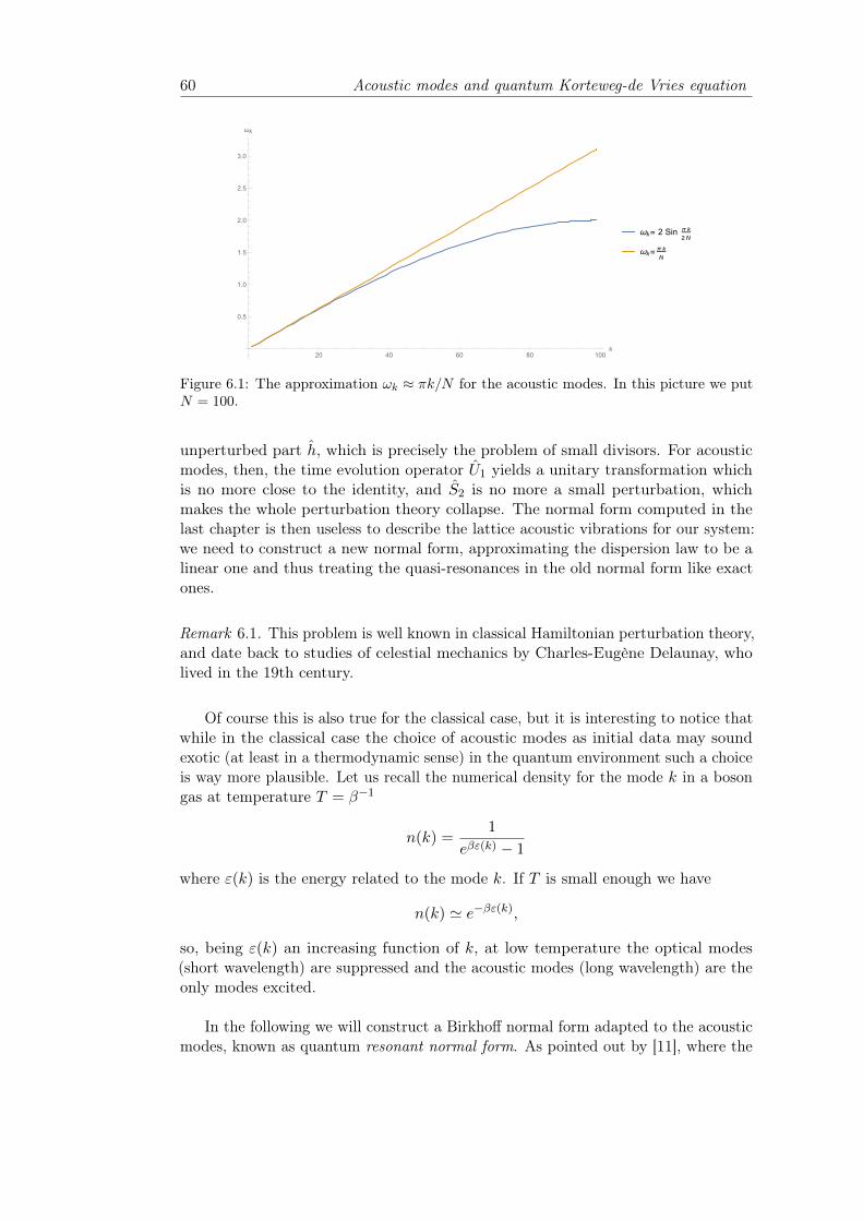
60 Acoustic modes and quantum Korteweg-de Vries equation

20 40 60 80 100k

0.5

1.0

1.5

2.0

2.5

3.0

ωk

ωk= 2 Sinπ k

2N

ωk=π k

N

Figure 6.1: The approximation ωk ≈ πk/N for the acoustic modes. In this picture we putN = 100.

unperturbed part h, which is precisely the problem of small divisors. For acousticmodes, then, the time evolution operator U1 yields a unitary transformation whichis no more close to the identity, and S2 is no more a small perturbation, whichmakes the whole perturbation theory collapse. The normal form computed in thelast chapter is then useless to describe the lattice acoustic vibrations for our system:we need to construct a new normal form, approximating the dispersion law to be alinear one and thus treating the quasi-resonances in the old normal form like exactones.

Remark 6.1. This problem is well known in classical Hamiltonian perturbation theory,and date back to studies of celestial mechanics by Charles-Eugène Delaunay, wholived in the 19th century.

Of course this is also true for the classical case, but it is interesting to notice thatwhile in the classical case the choice of acoustic modes as initial data may soundexotic (at least in a thermodynamic sense) in the quantum environment such a choiceis way more plausible. Let us recall the numerical density for the mode k in a bosongas at temperature T = β−1

n(k) =1

eβε(k) − 1

where ε(k) is the energy related to the mode k. If T is small enough we have

n(k) ' e−βε(k),

so, being ε(k) an increasing function of k, at low temperature the optical modes(short wavelength) are suppressed and the acoustic modes (long wavelength) are theonly modes excited.

In the following we will construct a Birkhoff normal form adapted to the acousticmodes, known as quantum resonant normal form. As pointed out by [11], where the

Construction of the quantum resonant normal form 61

classical problem is studied, a suitable rescaling transforms the Hamilton equationsfor this type of normal form (of the classical FPU problem) into the so-called Fourier-Galerkin truncation to N − 1 modes of the 2N periodic Korteweg-de Vries equation(in the following denoted by KdV)

Ut =1

24Uxxx +

α√2UUx (6.1)

with periodic boundary conditions

U(x+ L, t) = U(x, t), ∀x, t ∈ R, L = 2N.

Our aim is to study the quantum problem and see the analogous of the KdV equation,which will be the equivalent of the Heisenberg equations for the creation operator.

6.2 Construction of the quantum resonant normal form

The core of the method resides in the expansion of the dispersion relation

ωk = ξk −1

24ξ3k +O(ξ5

k), ξk =πk

N

clearly adapted to the acoustic modes. The quadratic part h of the qFPU Hamiltonianoperator is now split

N−1∑k=1

ωka†kak =

N−1∑k=1

ξka†kak +

N−1∑k=1

(−ξ3k

24+ . . .)a†kak.

For initial excitation of acoustic modes, the sum

J(a, a†) :=

N−1∑k=1

ξka†kak

is regarded as the unperturbed part of the Hamiltonian operator, while the perturba-tion is given by

− 1

24

N−1∑k=1

ξ3ka†kak +

α

4√N

B(N)∑k=1

√ξ2kξ2k−N (a2k + a†2k)+

+α

12√N

N−1∑k1,k2,k3=1

√ξk1ξk2ξk3∆3(k1, k2, k3)[ak1ak2ak3+

+ 3a†k1ak2ak3 + 3a†k1

a†k2ak3 + a†k1

a†k2a†k3

].

A step of normalization (in the sense of perturbation theory) will be performed, withthe flow of the unperturbed part given by

ak(t) = e−iξktak, a†k(t) = eiξkta†k, ∀k = 1, . . . , N − 1.


While the quadratic term coincides with its average, and the linear term averagesto zero, the new first order perturbation is no longer zero because of the acousticdispersion law. In fact the average along the flow of J is obtained with the samemethod above and is given by

S1,res = − 1

24

N−1∑k=1

ξ3ka†kak +

α

4√N

N−1∑j,l,m=1

√ξjξlξm(a†jalamδj,l+m + a†ja

†l amδj+l,m)

Proposition 6.1. The first order resonant Birkhoff normal form for the qFPUHamiltonian operator is, neglecting the remainder,

R(a, a†) =N−1∑k=1

ξka†kak −

1

24

N−1∑k=1

ξ3ka†kak

+α

4√N

N−1∑j,l,m=1


†l amδj+l,m) (6.2)

It is interesting to explicitly verify that [h, S1,res] = 0. Clearly [h, 124

∑N−1k=1 ξ3

ka†kak] =

0, so we only have to compute [h, α4√N

∑jlm


†l amδj+l,m].

Being [nk, aq] = −δk,qak and [nk, a†q] = δk,qa

†k one has

[nk, a†jalam] = [nk, a

†j ]alam + a†j [nk, alam] = δk,ja

†kalam − δk,ma

†jalam − δk,la

†jalam

[nk, a†ja†l am] = [nk, a

†ja†l ]am + a†ja

†l [nk, am] = δk,la

†ja†l am + δk,ja

†ja†l am − δk,ma

†ja†l am.

So we have

α

4√N

∑kjlm

ξk√ξjξlξm[a†kalamδj,l+m(δk,jδk,m − δk,l) + a†ja

†l amδj+l,m(δk,l + δk,j − δk,m)]

=α

4√N

∑jlm

[a†jalamδj,l+m

(ξ

3/2j

√ξlξm − ξ3/2

m

√ξjξl − ξ

3/2l

√ξjξm

)+ a†ja

†l amδj+l,m

(ξ

3/2l

√ξjξm + ξ

3/2j

√ξlξm − ξ3/2

m

√ξjξl)]

=α

4√N

∑jlm

[a†l+malam

(ξ

3/2l+m

√ξlξm − ξ3/2

m

√ξl+mξl − ξ

3/2l

√ξl+mξm

)+ a†ja

†l aj+l

(ξ

3/2l

√ξjξj+l + ξ

3/2j

√ξlξj+l − ξ

3/2j+l

√ξjξl)].

Now, being ξl+m = ξl + ξm, it is easy to verify that

ξ3/2l+m

√ξlξm = ξ3/2

m

√ξl+mξl + ξ

3/2l

√ξl+mξm ∀l,m = 1, . . . , N − 1

so that [h, S1,res] = 0.

Towards the quantum KdV equation 63

6.3 Towards the quantum KdV equation

The Heisenberg equation for the creation operator ak, k = 1, . . . , N − 1, evolvingin time with the dynamics given by R is

ak = −i[ak, R]

= −iξkak +i

24ξ3kak −

iα

4√N

N−1∑j,l,m=1

√ξjξlξm([ak, a

†jalam]δj,l+m + [ak, a

†ja†l am]δj+l,m)

= −iξkak +i

24ξ3kak+

− iα

4√N

N−1∑j,l,m=1

√ξjξlξm(alamδk,jδj,l+m + a†l amδk,jδj+l,m + a†jamδk,lδj+l,m)

so finally one has

ak = −iξkak +i

24ξ3kak −

iα√ξk

4√N

N−1∑l,m=1

√ξlξm(alamδk,l+m + 2a†l amδk+l,m).

The Heisenberg equations for the creation operators are

a†k = iξka†k −

i

24ξ3ka†k +

iα√ξk

4√N

N−1∑l,m=1

√ξlξm(a†l a

†mδk,l+m + 2a†l amδk+l,m).

We wish now to polish this equation up and put it in a suitable form. Our first stepis to introduce the so-called co-rotating coordinates, which are

ak = e−iξktzk, a†k = eiξktz†k, ∀k = 1, . . . , N − 1.

The new coordinates zk and z†k do not commute, in fact

[zk, z†k′ ] = [eiξktak, e

−iξk′ ta†k′ ] = ei(ξk−ξk′ )t[ak, a†k] = δk,k′

which makes the transformation canonical. Being ak = −iξkak + e−iξktzk theHeisenberg equations for ak and a†k become

zk =i

24ξ3kzk −

iα√ξk

4√N

N−1∑l,m=1

√ξlξm(zlzmδk,l+m + 2z†l zmδk+l,m)

z†k = − i

24ξ3kz†k +

iα√ξk

4√N

N−1∑l,m=1

√ξlξm(z†l z

†mδk,l+m + 2z†l zmδk+l,m).

The second and final step is a non-canonical rescaling together with an exchange ofthe creation and annihilation operators

uk =√ξkz†k, ∀k = 1, . . . , N − 1, [uk, u

†k′ ] = −ξkδkk′

which leads us to the following result.


Proposition 6.2. The Heisenberg equation for the creation operator a†k for theacoustic modes of the qFPU problem is equivalent to

uk = − i

24ξ3kuk +

iαξk

4√N

N−1∑l,m=1

(ulumδk,l+m + 2u†lumδk+l,m) (6.3)

with [uk, u†k′ ] = −ξkδk,k′.

Remark 6.2. This equation is the one obtained in [11], where instead of commutingcoordinates uk, u∗k ∈ C we have non-commuting operators uk, u

†k.

There is a strong connection between this last equation and the so called quantumKdV equation (in the following qKdV)

ψt =1

24ψxxx +

α

2√

2(ψψx + ψxψ) (6.4)

where ψ(x, t) is a L-periodic hermitian field operator such that [ψ(x, t), ψ(x′, t)] =iδx(x− x′) where δx is the weak derivative of the delta distributions with respect tothe x variable.

Definition 6.1 (Fourier-Galerkin truncation). The Fourier-Galerkin truncation tothe first N modes of a L-periodic field operator U(x, t) is

1√L

N∑k=−N

Uk(t)e2πikxL ,

where Uk(t) = L−1/2∫ L

0 U(x, t)e−2πikxL dx.

Theorem 6.1. The normal form (6.3) coincide with the Fourier-Galerkin truncationto the first N − 1 modes of the qKdV equation (6.4)

ψt =1

24ψxxx +

α

2√

2(ψψx + ψxψ),

with periodic zero-average initial datum, namely

ψ(x+ L, 0) = ψ(x, 0),

∫ L

0ψ(x, 0) dx = 0,

where L = 2N .

Proof. Consider the qKdV equation (6.4). The field ψ(x, t) admits the Fourierexpansion

ψ(x, t) =1√L

∑k∈Z\0

Uk(t)e2πikxL ,

with Uk(t) = 1√L

∫ L0 ψ(x, t)e−

2πikxL and U−k(t) = U †k(t), where we impose the com-

mutation rule[Uk(t), U

†q (t)] = −ξkδk,q.

Towards the quantum KdV equation 65

One immediately finds

ψt =1√L

∑k

dUkdt

e2πikxL , ψxxx =

1√L

∑k

[(2πik

L

)3

Uk

]e

2πikxL ,

as well as

1

2(ψxψ + ψψx) =

1

2

∂

∂xψ2 =

∂

∂x

1

2L

∑q,p

UpUqe2πi(q+p)x

L

=1√L

∑k

[2πik

L

1

2√L

∑q,p

UpUqδk,q+p

]e

2πikxL .

.

Thus, the generic Fourier coefficient Uk evolves according to

dUkdt

= − i

24

(2πk

L

)3

Uk +2πk

L

iα

2√

2L

∑q,p∈Z\0

UpUqδk,q+p. (6.5)

Let us rewrite in a suitable way the convolution at the right hand side of the lastequation.

∑q∈Z\0

Uk−qUq =+∞∑q=1

Uk−qUq +−1∑

q=−∞Uk−qUq

=k−1∑q=1

Uk−qUq ++∞∑q=k+1

U−(q−k)Uq ++∞∑q=1

Uk+qU−q

=k−1∑q=1

Uk−qUq ++∞∑q=1

U †qUk+q ++∞∑q=1

Uk+qU†q

Being q 6= 0 U †qUk+q = Uk+qU†q , so the latter becomes

∑q∈Z\0

Uk−qUq =

k−1∑q=1

Uk−qUq + 2

+∞∑q=1

U †qUk+q

=k−1∑q=1

Uk−qUq + 2N−k−1∑q=1

U †qUk+q +

2+∞∑

q=N−kU †qUk+q

The Fourier-Galerkin truncation to the first N−1 modes consists exactly in neglectingthe contribution of the last quantity in the convolution above. Recalling that2L = N and 2πk/L = ξk, and renaming Uk(t) = uk(t), we have exactly (6.3). Thecommutation rule [ψ(x, t), ψ(x′, t)] = iδx(x − x′) derives directly from the one of


[uk(t), u†k′(t)] = −ξkδk,k′ with u−k = u†k. In fact

[ψ(x, t), ψ(x′, t)] =1

L

∑k

uk(t)eiξkx,

∑k′

uk′eiξk′x]

=1

L

∑k,k′

[uk, uk′ ]ei(ξkx+ξk′x

′)

= − 1

L

∑k,k′

ξkδk,−k′ei(ξkx+ξk′x

′)

= − 1

L

∑k

ξkeiξk(x−x′) = iδx(x− x′)

where we used δ(x) = 1L

∑k e

iξkx.

Remark 6.3. The classical construction is almost equivalent, with the usual differencethat in this work we are dealing with non-commuting operators instead of commutingcomplex coordinates. In the end, one finds that the acoustic modes, after anappropriate rescaling, obey to the Hamilton equations

uk = − i

24ξ3kuk +

iαξk

4√N

N−1∑l,m=1

(ulumδk,l+m + 2u∗l umδk+l,m)

where uk, u∗k′ = iξkδk,k′ . In [11] it was found that these equation are the Fourier-Galerkin truncation of the Korteweg-de Vries equation (6.1), with U(x), U(y) =δx(x− y).

6.4 Integrability of the quantum KdV equation

Thanks to theorem 6.1, we can state that, in first approximation, systems like theone studied in [3] have dynamics close to the one described by the qKdV equation (6.4).In order to understand why such systems do not show thermalisation, studying theintegrability property of this equation seems of the uttermost importance. We mustremark, however, that we actually don’t know neither what quantum thermalisationis, nor how integrability affects the thermalisation properties of our physical system.On the other hand, we think (guided by semi-classic arguments) that there is somekind of connection between the presence of an infinite number of conserved quantitiesfor a quantum system, and thus its integrability, and its lack of thermalisation. Theequation (6.4) is already present in literature, for example in [6], where it is obtainedfrom the quantization of the classical KdV, and its integrability is studied using the socalled theory of hereditary operators. In the following we will show how integrabilityis obtained, but we will not enter in such a vast world as the one of the nonlinearevolution equations for quantum operators.

In order to provide the quantum KdV equation (6.4) an Hamiltonian formulation,we must put it in an algebraic environment which is the one of almost-boundeddistributions.

Integrability of the quantum KdV equation 67

Definition 6.2 (Almost-bounded distribution). A distribution φ(x) is said to bealmost-bounded if, for every n ∈ N, its n-th derivative is of the form

φ(n)(x) = b(x) + ∆(x)

where b is locally bounded and where ∆ is a distribution with discrete support suchthat the support has no accumulation point.

Consider the algebra fulfilling the commutation rule

[u(x), u(x)] = iδx(x− x)

by taking suitable congruence classes in the algebra of the almost-bounded distribu-tions of degree 3. We will call this algebra QF .

Since elements of QF may be considered as operators (by multiplication) on QFitself, we have found the required operator representation of the Poisson structure ofthe quantum KdV. Now, we have the prerequisites to define the time evolution forquantum systems by taking suitable Hamiltonian operators. For example, taking

H =

∫(u(ξ)u(ξ)u(ξ)− 1

2uξ(ξ)uξ(ξ)) dξ

and defining the action of a commutator on an integral, as integral in the convolutionsense over the commutator with its integrand, we find

u(x)t = −i[u(x), H] = uxxx(x) + 3ux(x)u(x) + 3u(x)ux(x) (6.6)

which is, up to multiplicative constants, the equation we found in the previouschapter. This equation is considered in [6] as the quantum version of KdV. The mainproblem is to prove that this equation is completely integrable in the usual sense,i.e. that it has infinitely many commuting symmetry groups (or conserved quantitiesin involution). In order to give a recursive description of the symmetries and theconserved quantities of the quantum KdV (6.6), an alternative representation of itsdynamics is introduced. Define the space of densities to be QF where integrals overtotal derivatives are ignored (see [6]). This is exactly our case, since we are dealingwith the quantum Korteweg de Vries equation with periodic boundary conditions,and u(x+ L) = u(x) ∀x.

Let A and B two elements in QF . Define for all A,B ∈ QF an inner product inQF by

〈A,B〉 :=

∫TL

A(x)B(x) dx

where the integration is performed in TL, since we have imposed periodic boundaryconditions.Remark 6.4. The differential operator D is antisymmetric with respect to thatdensity-valued inner product.

Let F = F (u) a density depending in some way on the field variable u. Thendefine its directional derivative of F in the direction of an element B of QF by

F ′[B] =∂

∂εF (u+ εB)|ε=0.


These definitions, and the notion of density, provide as simple result that there is aunique operator ∇, mapping densities into density-valued linear functionals on QFsuch that

F ′[B] = 〈∇F,B〉 for all B ∈ QF.

The quantity ∇F is said to be the gradient of F . For example, one obtains thegradient of

H1 =

∫TL

(u(ξ)u(ξ)u(ξ)− 1

2uξ(ξ)uξ(ξ)) dξ (6.7)

as uxx(x) + 3u(x)u(x). The quantum KdV equation (6.6) can now be rewritten as

ut = D∇H1

where H1 is given above in (6.7), and D denotes the operator of taking the derivativewith respect to x which is an implectic operator (the equivalent of a Poisson tensor,in this notation). This equation has a very special property, like the classical case,which is that it can be endowed with two different Hamiltonian structure, i.e. twodifferent Poisson tensors J1 and J2 and two different Hamiltonians H1 and H2 suchthat the equation can be read as ut = J1∇H1 = J2∇H2. We have just seen the firstHamiltonian formulation, that is

J1 = D H1 =

∫TL

(u(ξ)u(ξ)u(ξ)− 1

2uξ(ξ)uξ(ξ)) dξ

which is the equivalent of the first Hamiltonian formulation of the classical KdVequation (see [20] for details).

We are now ready to derive the second Hamiltonian formulation of the quantumKdV (6.6). Denote by u the field variable and introduce

L(u)A := uA, R(u)A := Au

where A ∈ QF . These are operators of multiplication with u from the left and fromthe right. Then set

Θ = D3 +DL(u) +DR(u) +R(u)D + L(u)D + [L(u)−R(u)]D−1[L(u)−R(u)]

which gives an operator being antisymmetric with respect to the inner productdefined above. It is possible (but arduous) to verify that Θ is an implectic operator(i.e. a Poisson tensor), and thus provides the second Hamiltonian formulation of(6.6), with Hamiltonian

H2 =1

2

∫TL

u(ξ)u(ξ) dξ (6.8)

then we have ∇H2 = u whenceut = Θ∇H2

is again the quantum KdV flow. It’s easy to verify that in the commutative case,where R(u) = L(u), this second implectic operator of the quantum KdV is equivalentto the second Poisson tensor of the KdV.Now [6] apply the theory of hereditary operators of [7] and [8] in order to have arecursive generation of conserved densities and vector fields. It is proven, using

Integrability of the quantum KdV equation 69

Bäcklund transformations, that the two implectic operators are compatible (i.e. theirsum is again an implectic operator), so

Φ = ΘD−1

is an hereditary and a strong symmetry. Qualitatively, if K(u) is the quantum KdVvector field, then

– a symmetry is a vector field S(u) such that [K,S] = K ′[S]− S′[K] = 0;

– a strong symmetry is an operator-valued function Φ which maps symmetries ofut = K(u) into symmetries of that equation;

– an hereditary symmetry is an operator-valued function Φ such that if it is astrong symmetry of any equation ut = K(u), then it is a strong symmetry alsofor ut = Φ(u)K(u).

and generates out of the vector field of the quantum KdV a hierarchy of commutingflows Φn(u)K(u), n ∈ Z, which constitute the symmetry group generators for thequantum KdV since it is among the members of the hierarchy. For the equivalentof Noether’s theorem, these commuting symmetries produce an infinite number ofconserved quantities in involution, which cause the integrability of the quantumKorteweg-de Vries equation in the same way as the classical case.

We want to remark that, although this fact is surely of mathematical and formalinterest, we don’t actually know the physical effects and consequences on the quantumFermi-Pasta-Ulam system and its thermalisation. If this was a classical system, thenits integrability should prevent ergodicity and then thermalisation, at least for along period of time. However, this is a quantum system, and as we already pointedout, there isn’t a real and solid theory of quantum thermalisation yet. The fact thatthe theory of nonlinear quantum evolution equations is a wide and complex field,and that there is not a real physical application of it, are the reasons why we didn’tdedicate much space in this work on the study of this equation’s integrability. Theaim of this section was only to pointing out that the quantum Korteweg-de Vriesequation, which describes the quantum FPU system for a long period of time, wasalready studied from a mathematical point of view and its integrability was proven.


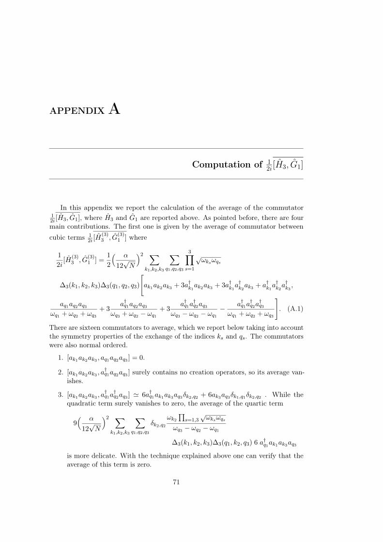
APPENDIX A

Computation of 12i [H3, G1]

In this appendix we report the calculation of the average of the commutator12i [H3, G1], where H3 and G1 are reported above. As pointed before, there are fourmain contributions. The first one is given by the average of commutator betweencubic terms 1

2i [H(3)3 , G

(3)1 ] where

1

2i[H

(3)3 , G

(3)1 ] =

1

2

( α

12√N

)2 ∑k1,k2,k3

∑q1,q2,q3

3∏s=1

√ωksωqs

∆3(k1, k2, k3)∆3(q1, q2, q3)

[ak1ak2ak3 + 3a†k1

ak2ak3 + 3a†k1a†k2

ak3 + a†k1a†k2

a†k3,

aq1aq2aq3ωq1 + ωq2 + ωq3

+ 3a†q1aq2aq3

ωq3 + ωq2 − ωq1+ 3

a†q1a†q2aq3

ωq3 − ωq2 − ωq1− a†q1a

†q2a†q3

ωq1 + ωq2 + ωq3

]. (A.1)

There are sixteen commutators to average, which we report below taking into accountthe symmetry properties of the exchange of the indices ks and qs. The commutatorswere also normal ordered.

1. [ak1ak2ak3 , aq1aq2aq3 ] = 0.

2. [ak1ak2ak3 , a†q1aq2aq3 ] surely contains no creation operators, so its average van-

ishes.

3. [ak1ak2ak3 , a†q1a†q2aq3 ] ' 6a†q1ak1ak3aq3δk2,q2 + 6ak3aq3δk1,q1δk2,q2 . While the

quadratic term surely vanishes to zero, the average of the quartic term

9( α

12√N

)2 ∑k1,k2,k3

∑q1,q2,q3

δk2,q2

ωk2

∏s=1,3

√ωksωqs

ωq3 − ωq2 − ωq1

∆3(k1, k2, k3)∆3(q1, k2, q3) 6 a†q1ak1ak3aq3

is more delicate. With the technique explained above one can verify that theaverage of this term is zero.

71

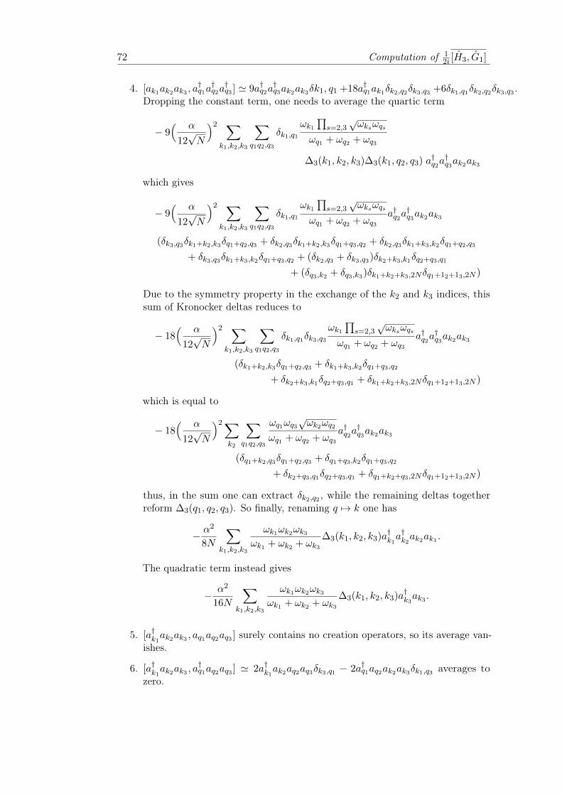
72 Computation of 12i [H3, G1]

4. [ak1ak2ak3 , a†q1a†q2a†q3 ] ' 9a†q2a

†q3ak2ak3δk1, q1 +18a†q1ak1δk2,q2δk3,q3 +6δk1,q1δk2,q2δk3,q3 .

Dropping the constant term, one needs to average the quartic term

− 9( α

12√N

)2 ∑k1,k2,k3

∑q1q2,q3

δk1,q1

ωk1

∏s=2,3

√ωksωqs

ωq1 + ωq2 + ωq3

∆3(k1, k2, k3)∆3(k1, q2, q3) a†q2a†q3ak2ak3

which gives

− 9( α

12√N

)2 ∑k1,k2,k3

∑q1q2,q3

δk1,q1

ωk1

∏s=2,3

√ωksωqs

ωq1 + ωq2 + ωq3a†q2a

†q3ak2ak3

(δk3,q3δk1+k2,k3δq1+q2,q3 + δk2,q3δk1+k2,k3δq1+q3,q2 + δk2,q3δk1+k3,k2δq1+q2,q3

+ δk3,q3δk1+k3,k2δq1+q3,q2 + (δk2,q3 + δk3,q3)δk2+k3,k1δq2+q3,q1

+ (δq3,k2 + δq3,k3)δk1+k2+k3,2Nδq1+12+13,2N )

Due to the symmetry property in the exchange of the k2 and k3 indices, thissum of Kronocker deltas reduces to

− 18( α

12√N

)2 ∑k1,k2,k3

∑q1q2,q3

δk1,q1δk3,q3

ωk1

∏s=2,3

√ωksωqs


†q3ak2ak3

(δk1+k2,k3δq1+q2,q3 + δk1+k3,k2δq1+q3,q2

+ δk2+k3,k1δq2+q3,q1 + δk1+k2+k3,2Nδq1+12+13,2N )

which is equal to

− 18( α

12√N

)2∑k2

∑q1q2,q3

ωq1ωq3√ωk2ωq2


†q3ak2ak3

(δq1+k2,q3δq1+q2,q3 + δq1+q3,k2δq1+q3,q2

+ δk2+q3,q1δq2+q3,q1 + δq1+k2+q3,2Nδq1+12+13,2N )

thus, in the sum one can extract δk2,q2 , while the remaining deltas togetherreform ∆3(q1, q2, q3). So finally, renaming q 7→ k one has

− α2

8N

∑k1,k2,k3

ωk1ωk2ωk3

ωk1 + ωk2 + ωk3

∆3(k1, k2, k3)a†k1a†k2

ak2ak1 .

The quadratic term instead gives

− α2

16N

∑k1,k2,k3

ωk1ωk2ωk3

ωk1 + ωk2 + ωk3

∆3(k1, k2, k3)a†k3ak3 .

5. [a†k1ak2ak3 , aq1aq2aq3 ] surely contains no creation operators, so its average van-

ishes.

6. [a†k1ak2ak3 , a

†q1aq2aq3 ] ' 2a†k1

ak2aq2aq3δk3,q1 − 2a†q1aq2ak2ak3δk1,q3 averages tozero.

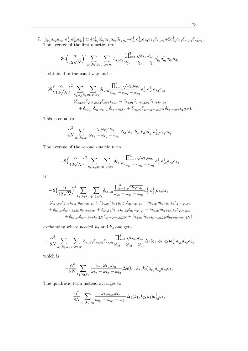
73

7. [a†k1ak2ak3 , a

†q1a†q2aq3 ] ' 4a†k1

a†q1ak3aq3δk2,q2−a†q1a†q2ak2ak3δk1,q3+2a†k3

aq3δk1,q1δk2,q2 .The average of the first quartic term

36( α

12√N

)2 ∑k1,k2,k3

∑q1,q2,q3

δk2,q2

∏3s=1√ωksωqs

ωq3 − ωq2 − ωq1a†k1

a†q1ak3aq3

is obtained in the usual way and is

36( α

12√N

)2 ∑k1,k2,k3

∑q1,q2,q3

δk2,q2

∏3s=1√ωksωqs

ωq3 − ωq2 − ωq1a†k1

a†q1ak3aq3

(δk3,q1δq1+q2,q3δk2+k3,k1 + δk3,q1δq1+q3,q2δk1+k3,k2

+ δk3,q1δq2+q3,q1δk1+k2,k3 + δk3,q1δq1+q2+q3,2Nδk1+k2+k3,2N ).

This is equal to

α2

4N

∑k1,k2,k3

ωk1ωk2ωk3


∆3(k1, k2, k3)a†k1a†k3

ak3ak1 .

The average of the second quartic term

−9( α

12√N

)2 ∑k1,k2,k3

∑q1,q2,q3

δk1,q3

∏3s=1√ωksωqs

ωq3 − ωq2 − ωq1a†q1a

†q2ak2ak3

is

− 9( α

12√N

)2 ∑k1,k2,k3

∑q1,q2,q3

δk1,q3

∏3s=1√ωksωqs

ωq3 − ωq2 − ωq1a†q1a

†q2ak2ak3

(δk2,q2δk2+k3,k1δq1+q2,q3 + δk3,q2δk2+k3,k1δq1+q2,q3 + δk3,q2δk1+k2,k3δq1+q3,q2

+ δk2,q2δk1+k3,k2δq1+q3,q2 + δk2,12δk1+k2,k3δq2+q3,q1 + δk3,q2δk1+k3,k2δq2+q3,q1

+ δk2,q2δk1+k2+k3,2Nδq1+q2+q3,2N + δk3,q2δk1+k2+k3,2Nδq1+q2+q3,2N )

exchanging where needed k2 and k3 one gets

− α2

8N

∑k1,k2,k3

∑q1,q2,q3

δk1,q3δk2,q2δk3,q1

∏3s=1√ωksωqs

ωq3 − ωq2 − ωq1∆3(q1, q2, q3)a†q1a

†q2ak2ak3

which is

− α2

8N

∑k1,k2,k3

ωk1ωk2ωk3


∆3(k1, k2, k3)a†k1a†k2

ak2ak1 .

The quadratic term instead averages to

α2

8N

∑k1,k2,k3

ωk1ωk2ωk3


∆3(k1, k2, k3)a†k3ak3 .


8. [a†k1ak2ak3 , a

†q1a†q2a†q3 ] ' 6a†k1

a†q1a†q2ak2δk3,q3 + 6a†k1

a†q1δk3,q3δk2,q2 averages tozero.

9. [a†k1a†k2

ak3 , aq1aq2aq3 ] ' −6a†k2aq2aq3ak3δk1,q1 − 6aq3ak3δk1,q1δk2,q2 as the third

contribution averages to zero.

10. [a†k1a†k2

ak3 , a†q1aq2aq3 ] ' a†k1

a†k2aq2aq3δk3,q1−4a†q1a

†k1aq3ak3δk2,q2−2a†q1ak3δq2,k2δk1,q3 .

Its average can be computed in the same way of the seventh contribution, andgives the exact same contribution

11. [a†k1a†k2

ak3 , a†q1a†q2aq3 ] ' 2a†k1

a†k2a†q2aq3δk3,q1 − 2a†q1a

†q2a†k2ak3δk1,q3 averages to

zero.

12. [a†k1a†k2

ak3 , a†q1a†q2a†q3 ] surely contains no annihilation operators, so its average

vanishes.

13. [a†k1a†k2

a†k3, aq1aq2aq3 ] ' −9a†k1

a†k2aq1aq2δk3,q3−18a†k1

aq1δk2,q2δk1, q1−6δk1,q1δk2, q2δk3,q3 .Its average can be computed in the same way of the fourth contribution andgives the exact same contribution.

14. [a†k1a†k2

a†k3, a†q1aq2aq3 ] ' −6a†q1a

†k1a†k2

aq2δk3,q3 − 6a†q1a†k1δq2,k2 |deltaq3,k3 as the

eighth contribution averages to zero.

15. [a†k1a†k2

a†k3, a†q1a

†q2aq3 ] surely contains no annihilation operators, so its average

vanishes.

16. [a†k1a†k2

a†k3, a†q1a

†q2a†q3 ] = 0.

Finally we get

1

2i[H

(3)3 , G

(3)1 ] = − α

2

4N

∑k1,k2,k3

ωk1ωk2ωk3

ωk1 + ωk2 + ωk3

∆3(k1, k2, k3)a†k1a†k2

ak2ak1

α2

2N

∑k1,k2,k3

ωk1ωk2ωk3


∆3(k1, k2, k3)a†k1a†k3

ak3ak1

− α2

4N

∑k1,k2,k3

ωk1ωk2ωk3


∆3(k1, k2, k3)a†k1a†k2

ak2ak1

+α2

8N

∑k1,k2,k3

ωk1ωk2ωk3

ωk1 + ωk2 + ωk3

∆3(k1, k2, k3)a†k3ak3

− α2

4N

∑k1,k2,k3

ωk1ωk2ωk3


∆3(k1, k2, k3)a†k3ak3 .

75

Renaming properly the indices we get the result (modulo constant terms)

1

2i[H

(3)3 , G

(3)1 ] =

α2

4N

∑k1,k2,k3


ak2ak1(2

1


− 1

ωk1 + ωk2 + ωk3

− 1


)

+α2

8N

∑k1,k2,k3


1

ωk1 + ωk2 + ωk3

− 21


)Now we show how to compute the average of

1

2i[H

(3)3 , G

(1)1 ] =

1

2i

[α

12√N

N−1∑k1,k2,k3=1

3∏s=1

√ωks∆3(k1, k2, k3)

(ak1ak2ak3 + 3a†k1ak2ak3 + 3a†k1

a†k2ak3 + a†k1

a†k2a†k3

),

α

4√N

B(N)∑q=1

(ωq − ωN−q)

[a†2qi√ω2q− a2q

i√ω2q

]]

starting from the commutators

1. [ak1ak2ak3 , a2q] = 0.

2. [a†k1ak2ak3 , a2q] surely contains no creation operators, so it averages to zero.

3. [a†k1a†k2

ak3 , a2q] = −δk1,2qa†k2ak3 − δk2,2qa

†k1ak3 .

4. [a†k1a†k2

a†k3, a2q] surely contains no annihilation operators, so it averages to zero.

5. [ak1ak2ak3 , a†2q] surely contains no creation operators, so it averages to zero.

6. [a†k1ak2ak3 , a

†2q] = a†k1

ak2δk3,2q + a†k1ak3δk2,2q.

7. [a†k1a†k2

ak3 , a†2q] surely contains no annihilation operators, so it averages to zero.

8. [a†k1a†k2

a†k3, a†2q] = 0.

Remembering that a†jak = a†jakδj,k, putting all together and using the symmetryproperties of exchange of the indices k one obtains the result

1

2i[H

(3)3 , G

(1)1 ] = − α

2

8N

N−1∑k=1

B(N)∑q=1

ωk(ωq − ωN−q)(δk,q + δk+q,N )a†kak

The quantity 12i [H

(1)3 , G

(3)1 ] is obtained in a similar way and gives the exact same

contribution. 12i [H

(1)3 , G

(1)1 ] instead gives only constant terms.


Bibliography

[1] Fermi, E., Pasta, J., Ulam, S., Studies of non linear problems, Los-Alamos inter-nal report, document LA-1940 (1955). In: Enrico Fermi Collected Papers, vol.II, pp. 977-988, University of Chicago Press/Accad. Naz. Lincei, Chicago/Roma(1965).

[2] Zabusky, N.J., Kruskal, M.D., Interaction of "solitons" in a collisionless plasmaand the recurrence of initial states. Phys. Rev. Lett. 15, 240-243 (1965).

[3] Toshiya Kinoshita, Trevor Wenger & David S. Weiss, A quantum Newton’scradle. Nature 440, 900-903 (13 April 2006).

[4] Anatoli Polkovnikov, Krishnendu Sengupta, Alessandro Silva, Mukund Vengalat-tore, Nonequilibrium dynamics of closed interacting quantum systems. Reviewof Modern Physics 83, July-September 2011.

[5] Tim Langen, Remi Geiger, Maximilian Kuhnert, Bernhard Rauer, Joerg Schmied-mayer, Local emergence of thermal correlations in an isolated quantum many-bodysystem, Nature Physics 9, 640-643 (2013).

[6] Benno Fuchssteiner, A. Roy Chowdhury, A new Approach to the Quantum KdV,Chaos, Solitons and Fractals, 5, 2345-2355 (1995).

[7] B. Fuchssteiner, A.S. Fokas, Symplectic structures, their Bäcklund transforma-tions and hereditary symmetries, Physica D: Nonlinear Phenomena 4, Issue 1,47-66, (1981).

[8] B. Fuchssteiner, Application of hereditary symmetries to nonlinear evolutionequations, Nonlinear Analysis: Theory, Methods & Applications 3, Issue 6,849-862, (November 1979).

[9] V. Bazhanov, S. Lukyanov, A. Zamolodchikov, Integrable Structure of Confor-mal Field Theory, Quantum KdV Theory and Thermodynamic Bethe Ansatz,Commun.Math.Phys. 177, 381-398 (1996).

[10] Andreas Henrici, Thomas Kappeler, Results on Normal Forms for FPU Chains,Communications in Mathematical Physics, 278, Issue 1, 145-177 (February2008).

[11] Giancarlo Benettin, Roberto Livi, Antonio Ponno, The Fermi-Pasta-UlamProblem: Scaling Laws vs. Initial Conditions, Journal of Statistical Physics135, Issue 5, 873-893 (June 2009).

77

78 Bibliography

[12] Giancarlo Benettin, Helen Christodoulidi, Antonio Ponno, The Fermi-Pasta-Ulam Problem and Its Underlying Integrable Dynamics, Journal of StatisticalPhysics 152, Issue 2, 195-212 (July 2013).

[13] Lax, P. D., Almost periodic solutions of the KdV equation. SIAM review, 18(3),412-459 (1976).

[14] Bogoljubov, N. N., On a New Method in the Theory of Superconductivity, J.Exptl. Theoret. Phys. (U.S.S.R.) 34, 58-65 (January, 1958).

[15] Herbert Fröhlich, Interaction of electrons with lattice vibrations, Proceedingsof the Royal Society of London. Series A, Mathematical and Physical Sciences,Vol. 215, No. 1122 (Dec. 5, 1952), pp. 291-298.

[16] Dirac, P. A. M., The Principles of Quantum Mechanics, Oxford University Press1958.

[17] Ashcroft, Neil W., Mermin, N. David,Solid State Physics, Harcourt 1976.

[18] Giancarlo Benettin, Introduzione ai sistemi dinamici, appunti per il corso diFisica Matematica, 2001/2002, Università degli Studi di Padova.

[19] Antonio Ponno, Hamiltonian Mechanics, Lectures Notes 2014/2015, for PhysicsMaster degree, Università degli Studi di Padova.

[20] Matteo Gallone, Hydrodynamics of the FPU Problem and its Integrable Aspects,Tesi di laurea Magistrale in Fisica, Università degli Studi di Padova.

Documents

The quantum Fermi Pasta Ulam problem - unipd.ittesi.cab.Unipd.it/53523/1/Tesi_LM_Stoppato.pdfAbstract In this work we consider the quantum version of the classical Fermi-Pasta-Ulam