The qcmetrics infrastructure for quality control andautomatic reporting

Laurent Gatto∗

Computational Proteomics Unit†

University of Cambridge, UK

May 15, 2016

Abstract

The qcmetrics package is a framework that provides simple data containers for quality metricsand support for automatic report generation. This document briefly illustrates the core datastructures and then demonstrates the generation and automation of quality control reports formicroarray and proteomics data.

Keywords: Bioinformatics, Quality control, reporting, visualisation

∗lg390@cam.ac.uk†http://cpu.sysbiol.cam.ac.uk

1

qcmetrics 2

Contents

1 Introduction 2

2 The QC classes 32.1 The QcMetric class . . . . . . . . . . . . . . . . . . . . . . . . . . . . . . . . . . . . 32.2 The QcMetrics class . . . . . . . . . . . . . . . . . . . . . . . . . . . . . . . . . . . 5

3 Creating QC pipelines 63.1 Microarray degradation . . . . . . . . . . . . . . . . . . . . . . . . . . . . . . . . . . 63.2 A wrapper function . . . . . . . . . . . . . . . . . . . . . . . . . . . . . . . . . . . . 93.3 Proteomics raw data . . . . . . . . . . . . . . . . . . . . . . . . . . . . . . . . . . . . 103.4 Processed 15N labelling data . . . . . . . . . . . . . . . . . . . . . . . . . . . . . . . . 14

4 Report generation 204.1 Custom reports . . . . . . . . . . . . . . . . . . . . . . . . . . . . . . . . . . . . . . . 204.2 New report types . . . . . . . . . . . . . . . . . . . . . . . . . . . . . . . . . . . . . . 24

5 QC packages 245.1 A simple RNA degradation package . . . . . . . . . . . . . . . . . . . . . . . . . . . . 245.2 A QC pipeline repository . . . . . . . . . . . . . . . . . . . . . . . . . . . . . . . . . . 25

6 Conclusions 25

1 Introduction

Quality control (QC) is an essential step in any analytical process. Data of poor quality can at bestlead to the absence of positive results or, much worse, false positives that stem from uncaught faultyand noisy data and much wasted resources in pursuing red herrings.

Quality is often a relative concept that depends on the nature of the biological sample, the experimentalsettings, the analytical process and other factors. Research and development in the area of QC hasgenerally lead to two types of work being disseminated. Firstly, the comparison of samples of variablequality and the identification of metrics that correlate with the quality of the data. These quality metricscould then, in later experiments, be used to assess their quality. Secondly, the design of domain-specificsoftware to facilitate the collection, visualisation and interpretation of various QC metrics is also anarea that has seen much development. QC is a prime example where standardisation and automationare of great benefit. While a great variety of QC metrics, software and pipelines have been describedfor any assay commonly used in modern biology, we present here a different tool for QC, whose mainfeatures are flexibility and versatility. The qcmetrics package is a general framework for QC that canaccommodate any type of data. It provides a flexible framework to implement QC items that storerelevant QC metrics with a specific visualisation mechanism. These individual items can be bundledinto higher level QC containers that can be readily used to generate reports in various formats. As aresult, it becomes easy to develop complete custom pipelines from scratch and automate the generation

qcmetrics 3

of reports. The pipelines can be easily updated to accommodate new QC items of better visualisationtechniques.

Section 2 provides an overview of the framework. In section 3, we use microarray (subsection 3.1)and proteomics data (subsection 3.3) to demonstrate the elaboration of QC pipelines: how to createindividual QC objects, how to bundle them to create sets of QC metrics and how to generate reports inmultiple formats. We also show how the above steps can be fully automated through simple wrapperfunctions in section 3.2. Although kept simple in the interest of time and space, these examples aremeaningful and relevant. In section 4, we provide more detail about the report generation process, howreports can be customised and how new exports can be contributed. We proceed in section 5 to theconsolidation of QC pipelines using Rand elaborate on the development of dedicated QC packages withqcmetrics.

2 The QC classes

The package provides two types of QC containers. The QcMetric class stores data and visualisationfunctions for single metrics. Several such metrics can be bundled into QcMetrics instances, that canbe used as input for automated report generation. Below, we will provide a quick overview of how tocreate respective QcMetric and QcMetrics instances. More details are available in the correspondingdocumentations.

2.1 The QcMetric class

A QC metric is composed of a description (name in the code chunk below), some QC data (qcdata)and a status that defines if the metric is deemed of acceptable quality (coded as TRUE), bad quality(coded as FALSE) or not yet evaluated (coded as NA). Individual metrics can be displayed as a shorttextual summary or plotted. To do the former, one can use the default show method.

library("qcmetrics")

qc <- QcMetric(name = "A test metric")

qcdata(qc, "x") <- rnorm(100)

qcdata(qc) ## all available qcdata

## [1] "x"

summary(qcdata(qc, "x")) ## get x

## Min. 1st Qu. Median Mean 3rd Qu. Max.

## -2.2150 -0.4942 0.1139 0.1089 0.6915 2.4020

show(qc) ## or just qc

## Object of class "QcMetric"

## Name: A test metric

## Status: NA

qcmetrics 4

## Data: x

status(qc) <- TRUE

qc

## Object of class "QcMetric"

## Name: A test metric

## Status: TRUE

## Data: x

Plotting QcMetric instances requires to implement a plotting method that is relevant to the data athand. We can use a plot replacement method to define our custom function. The code inside theplot uses qcdata to extract the relevant QC data from object that is then passed as argument toplot and uses the adequate visualisation to present the QC data.

plot(qc)

## Warning in x@plot(x, ...): No specific plot function defined

plot(qc) <-

function(object, ... ) boxplot(qcdata(object, "x"), ...)

plot(qc)

−2

−1

01

2

qcmetrics 5

2.2 The QcMetrics class

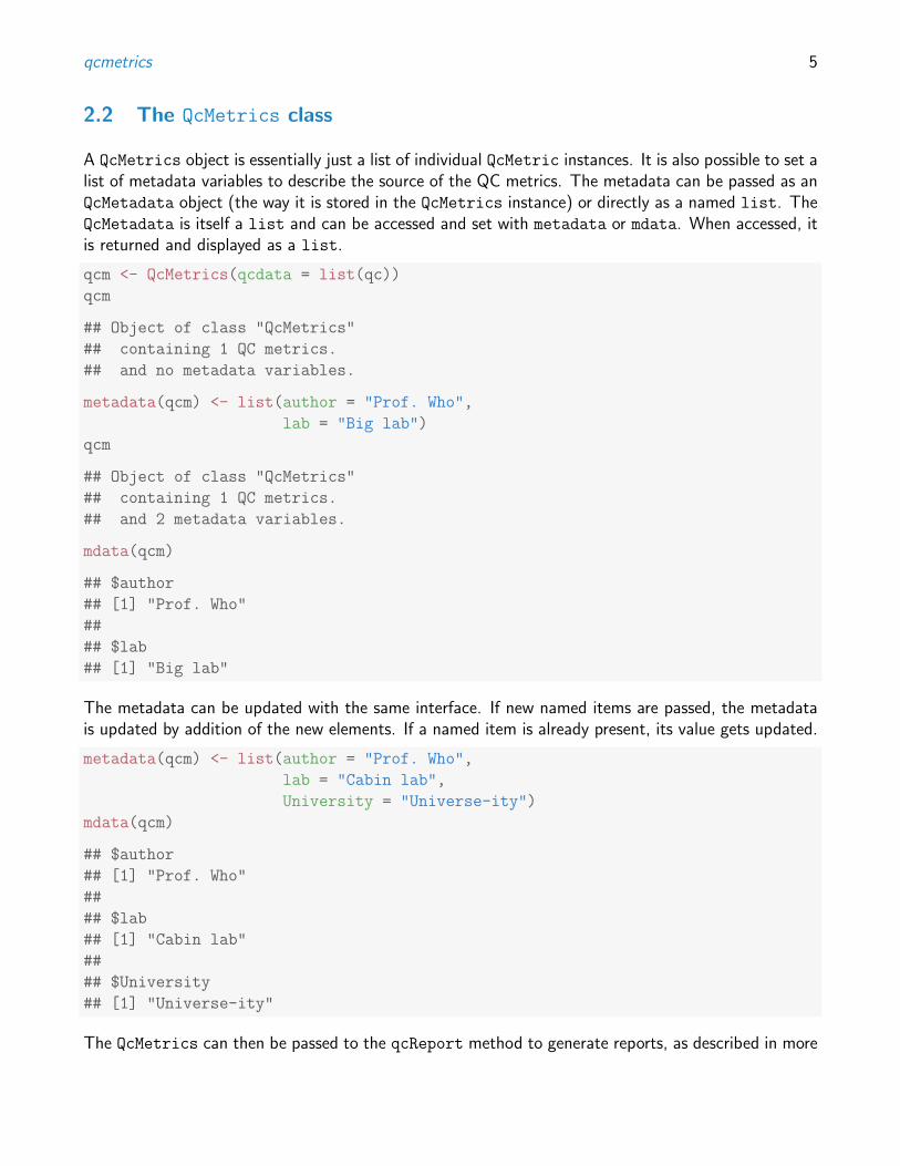
A QcMetrics object is essentially just a list of individual QcMetric instances. It is also possible to set alist of metadata variables to describe the source of the QC metrics. The metadata can be passed as anQcMetadata object (the way it is stored in the QcMetrics instance) or directly as a named list. TheQcMetadata is itself a list and can be accessed and set with metadata or mdata. When accessed, itis returned and displayed as a list.

qcm <- QcMetrics(qcdata = list(qc))

qcm

## Object of class "QcMetrics"

## containing 1 QC metrics.

## and no metadata variables.

metadata(qcm) <- list(author = "Prof. Who",

lab = "Big lab")

qcm

## Object of class "QcMetrics"

## containing 1 QC metrics.

## and 2 metadata variables.

mdata(qcm)

## $author

## [1] "Prof. Who"

##

## $lab

## [1] "Big lab"

The metadata can be updated with the same interface. If new named items are passed, the metadatais updated by addition of the new elements. If a named item is already present, its value gets updated.

metadata(qcm) <- list(author = "Prof. Who",

lab = "Cabin lab",

University = "Universe-ity")

mdata(qcm)

## $author

## [1] "Prof. Who"

##

## $lab

## [1] "Cabin lab"

##

## $University

## [1] "Universe-ity"

The QcMetrics can then be passed to the qcReport method to generate reports, as described in more

qcmetrics 6

details below.

3 Creating QC pipelines

3.1 Microarray degradation

We will use the refA Affymetrix arrays from the MAQCsubsetAFX package as an example data setand investigate the RNA degradation using the AffyRNAdeg from affy [1] and the actin and GAPDH3′

5′ratios, as calculated in the yaqcaffy package [2]. The first code chunk demonstrate how to load the

data and compute the QC data1.

library("MAQCsubsetAFX")

data(refA)

library("affy")

deg <- AffyRNAdeg(refA)

library("yaqcaffy")

yqc <- yaqc(refA)

We then create two QcMetric instances, one for each of our quality metrics.

qc1 <- QcMetric(name = "Affy RNA degradation slopes")

qcdata(qc1, "deg") <- deg

plot(qc1) <- function(object, ...) {x <- qcdata(object, "deg")

nms <- x$sample.names

plotAffyRNAdeg(x, col = 1:length(nms), ...)

legend("topleft", nms, lty = 1, cex = 0.8,

col = 1:length(nms), bty = "n")

}status(qc1) <- TRUE

qc1

## Object of class "QcMetric"

## Name: Affy RNA degradation slopes

## Status: TRUE

## Data: deg

qc2 <- QcMetric(name = "Affy RNA degradation ratios")

qcdata(qc2, "yqc") <- yqc

plot(qc2) <- function(object, ...) {par(mfrow = c(1, 2))

yaqcaffy:::.plotQCRatios(qcdata(object, "yqc"), "all", ...)

1The pre-computed objects can be directly loaded with load(system.file("extdata/deg.rda", package =

"qcmetrics")) and load(system.file("extdata/deg.rda", package = "qcmetrics")).

qcmetrics 7

}status(qc2) <- FALSE

qc2

## Object of class "QcMetric"

## Name: Affy RNA degradation ratios

## Status: FALSE

## Data: yqc

Then, we combine the individual QC items into a QcMetrics instance.

maqcm <- QcMetrics(qcdata = list(qc1, qc2))

maqcm

## Object of class "QcMetrics"

## containing 2 QC metrics.

## and no metadata variables.

With our QcMetrics data, we can easily generate quality reports in several different formats. Below,we create a pdf report, which is the default type. Using type = "html" would generate the equivalentreport in html format. See ?qcReport for more details.

qcReport(maqcm, reportname = "rnadeg", type = "pdf")

The resulting report is shown below. Each QcMetric item generates a section named according to theobject’s name. A final summary section shows a table with all the QC items and their status. Thereport concludes with a detailed session information section.

In addition to the report, it is of course advised to store the actual QcMetrics object. This is mosteasily done with the Rsave/load and saveRDS/readRDS functions. As the data and visualisationmethods are stored together, it is possible to reproduce the figures from the report or further explorethe data at a later stage.

Quality control report generated with qcmetrics

biocbuild

May 15, 2016

1 Affy RNA degradation slopes

## Object of class "QcMetric"## Name: Affy RNA degradation slopes## Status: TRUE## Data: deg

RNA degradation plot

5' <−−−−−> 3' Probe Number

Mea

n In

tens

ity :

shift

ed a

nd s

cale

d

0 2 4 6 8 10

010

2030

4050

AFX_1_A2.CELAFX_2_A5.CELAFX_3_A1.CELAFX_4_A4.CELAFX_5_A2.CELAFX_6_A1.CEL

1

2 Affy RNA degradation ratios

## Object of class "QcMetric"## Name: Affy RNA degradation ratios## Status: FALSE## Data: yqc

●

1.5

2.0

2.5

beta−actin 3'/5'

AFX_6_A1.CEL

CV: 0.38

●

0.90

0.95

1.00

1.05

1.10

1.15

1.20

GAPDH 3'/5'

AFX_6_A1.CEL

CV: 0.11

2

3 QC summary

#### Attaching package: ’xtable’## The following object is masked from ’package:RforProteomics’:#### display

name status1 Affy RNA degradation slopes TRUE2 Affy RNA degradation ratios FALSE

4 Session information

• R version 3.3.0 (2016-05-03), x86_64-pc-linux-gnu

• Locale: LC_CTYPE=en_US.UTF-8, LC_NUMERIC=C, LC_TIME=en_US.UTF-8, LC_COLLATE=C,LC_MONETARY=en_US.UTF-8, LC_MESSAGES=en_US.UTF-8, LC_PAPER=en_US.UTF-8, LC_NAME=C,LC_ADDRESS=C, LC_TELEPHONE=C, LC_MEASUREMENT=en_US.UTF-8, LC_IDENTIFICATION=C

• Base packages: base, datasets, grDevices, graphics, methods, parallel, stats, stats4, utils

• Other packages: AnnotationDbi 1.34.2, Biobase 2.32.0, BiocGenerics 0.18.0, BiocParallel 1.6.2,IRanges 2.6.0, MAQCsubsetAFX 1.10.0, MSnbase 1.20.5, ProtGenerics 1.4.0, Rcpp 0.12.5,RforProteomics 1.10.0, S4Vectors 0.10.0, affy 1.50.0, gcrma 2.44.0, genefilter 1.54.2, knitr 1.13,mzR 2.6.2, qcmetrics 1.10.2, simpleaffy 2.48.0, xtable 1.8-2, yaqcaffy 1.32.0

• Loaded via a namespace (and not attached): BiocInstaller 1.22.2, BiocStyle 2.0.2, Biostrings 2.40.0,Category 2.38.0, DBI 0.4-1, GSEABase 1.34.0, MALDIquant 1.14, Matrix 1.2-6, Nozzle.R1 1.1-1,R.methodsS3 1.7.1, R.oo 1.20.0, R.utils 2.3.0, R6 2.1.2, RBGL 1.48.0, RColorBrewer 1.1-2,RCurl 1.95-4.8, RJSONIO 1.3-0, RSQLite 1.0.0, RUnit 0.4.31, XML 3.98-1.4, XVector 0.12.0,affyio 1.42.0, annotate 1.50.0, biocViews 1.40.0, bitops 1.0-6, codetools 0.2-14, colorspace 1.2-6,digest 0.6.9, doParallel 1.0.10, evaluate 0.9, foreach 1.4.3, formatR 1.4, ggplot2 2.1.0, graph 1.50.0,grid 3.3.0, gridSVG 1.5-0, gtable 0.2.0, highr 0.6, htmltools 0.3.5, httpuv 1.3.3, impute 1.46.0,interactiveDisplay 1.10.2, interactiveDisplayBase 1.10.3, iterators 1.0.8, lattice 0.20-33, limma 3.28.4,magrittr 1.5, mime 0.4, munsell 0.4.3, mzID 1.10.2, pander 0.6.0, pcaMethods 1.64.0, plyr 1.8.3,preprocessCore 1.34.0, reshape2 1.4.1, rpx 1.8.2, scales 0.4.0, shiny 0.13.2, splines 3.3.0, stringi 1.0-1,stringr 1.0.0, survival 2.39-4, tools 3.3.0, vsn 3.40.0, zlibbioc 1.18.0

3

qcmetrics 9

3.2 A wrapper function

Once an appropriate set of quality metrics has been identified, the generation of the QcMetrics instancescan be wrapped up for automation.

rnadeg

## function (input, status, type, reportname = "rnadegradation")

## {

## requireNamespace("affy")

## requireNamespace("yaqcaffy")

## if (is.character(input))

## input <- affy::ReadAffy(input)

## qc1 <- QcMetric(name = "Affy RNA degradation slopes")

## qcdata(qc1, "deg") <- affy::AffyRNAdeg(input)

## plot(qc1) <- function(object) {

## x <- qcdata(object, "deg")

## nms <- x$sample.names

## affy::plotAffyRNAdeg(x, cols = 1:length(nms))

## legend("topleft", nms, lty = 1, cex = 0.8, col = 1:length(nms),

## bty = "n")

## }

## if (!missing(status))

## status(qc1) <- status[1]

## qc2 <- QcMetric(name = "Affy RNA degradation ratios")

## qcdata(qc2, "yqc") <- yaqcaffy::yaqc(input)

## plot(qc2) <- function(object) {

## par(mfrow = c(1, 2))

## yaqcaffy:::.plotQCRatios(qcdata(object, "yqc"), "all")

## }

## if (!missing(status))

## status(qc2) <- status[2]

## qcm <- QcMetrics(qcdata = list(qc1, qc2))

## if (!missing(type))

## qcReport(qcm, reportname, type = type, title = "Affymetrix RNA degradation report")

## invisible(qcm)

## }

## <environment: namespace:qcmetrics>

It is now possible to generate a QcMetrics object from a set of CEL files or directly from an affybatch

object. The status argument allows to directly set the statuses of the individual QC items; these canalso be set later, as illustrated below. If a report type is specified, the corresponding report is generated.

maqcm <- rnadeg(refA)

status(maqcm)

qcmetrics 10

## [1] NA NA

## check the QC data

(status(maqcm) <- c(TRUE, FALSE))

## [1] TRUE FALSE

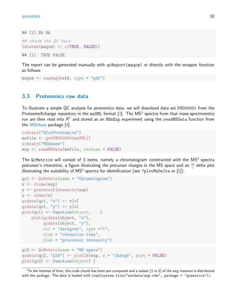
The report can be generated manually with qcReport(maqcm) or directly with the wrapper functionas follows:

maqcm <- rnadeg(refA, type = "pdf")

3.3 Proteomics raw data

To illustrate a simple QC analysis for proteomics data, we will download data set PXD00001 from theProteomeXchange repository in the mzXML format [3]. The MS2 spectra from that mass-spectrometryrun are then read into R2 and stored as an MSnExp experiment using the readMSData function fromthe MSnbase package [4].

library("RforProteomics")

msfile <- getPXD000001mzXML()

library("MSnbase")

exp <- readMSData(msfile, verbose = FALSE)

The QcMetrics will consist of 3 items, namely a chromatogram constructed with the MS2 spectraprecursor’s intensities, a figure illustrating the precursor charges in the MS space and an m

zdelta plot

illustrating the suitability of MS2 spectra for identification (see ?plotMzDelta or [5]).

qc1 <- QcMetric(name = "Chromatogram")

x <- rtime(exp)

y <- precursorIntensity(exp)

o <- order(x)

qcdata(qc1, "x") <- x[o]

qcdata(qc1, "y") <- y[o]

plot(qc1) <- function(object, ...)

plot(qcdata(object, "x"),

qcdata(object, "y"),

col = "darkgrey", type ="l",

xlab = "retention time",

ylab = "precursor intensity")

qc2 <- QcMetric(name = "MS space")

qcdata(qc2, "p2d") <- plot2d(exp, z = "charge", plot = FALSE)

plot(qc2) <- function(object) {2In the interest of time, this code chunk has been pre-computed and a subset (1 in 3) of the exp instance is distributed

with the package. The data is loaded with load(system.file("extdata/exp.rda", package = "qcmetrics")).

qcmetrics 11

require("ggplot2")

print(qcdata(object, "p2d"))

}

qc3 <- QcMetric(name = "m/z delta plot")

qcdata(qc3, "pmz") <- plotMzDelta(exp, plot = FALSE,

verbose = FALSE)

plot(qc3) <- function(object)

suppressWarnings(print(qcdata(object, "pmz")))

Note that we do not store the raw data in any of the above instances, but always pre-compute thenecessary data or plots that are then stored as qcdata. If the raw data was to be needed in multipleQcMetric instances, we could re-use the same qcdata environment to avoid unnecessary copies usingqcdata(qc2) <- qcenv(qc1) and implement different views through custom plot methods.

Let’s now combine the three items into a QcMetrics object, decorate it with custom metadata usingthe MIAPE information from the MSnExp object and generate a report.

protqcm <- QcMetrics(qcdata = list(qc1, qc2, qc3))

metadata(protqcm) <- list(

data = "PXD000001",

instrument = experimentData(exp)@instrumentModel,

source = experimentData(exp)@ionSource,

analyser = experimentData(exp)@analyser,

detector = experimentData(exp)@detectorType,

manufacurer = experimentData(exp)@instrumentManufacturer)

The status column of the summary table is empty as we have not set the QC items statuses yet.

qcReport(protqcm, reportname = "protqc")

Quality control report generated with qcmetrics

biocbuild

May 15, 2016

1 Metadata

data PXD000001

instrument LTQ Orbitrap Velos

source nanoelectrospray

analyser orbitrap

detector inductive detector

manufacurer Thermo Scientific

1

2 Chromatogram

## Object of class "QcMetric"## Name: Chromatogram## Status: NA## Data: x y

500 1000 1500 2000 2500 3000 3500

0e+

001e

+08

2e+

083e

+08

4e+

08

retention time

prec

urso

r in

tens

ity2

3 MS space

## Object of class "QcMetric"## Name: MS space## Status: NA## Data: p2d

## Loading required package: ggplot2

600

900

1200

1500

1000 2000 3000retention.time

prec

urso

r.mz

charge

2

3

4

5

6

3

4 m/z delta plot

## Object of class "QcMetric"## Name: m/z delta plot## Status: NA## Data: pmz

peg A RND

C EG HI/L K/Q M FPS T WYV

0.00

0.01

0.02

0.03

50 100 150 200m/z delta

Den

sity

Histogram of Mass Delta Distribution

4

5 QC summary

name status1 Chromatogram2 MS space3 m/z delta plot

6 Session information

• R version 3.3.0 (2016-05-03), x86_64-pc-linux-gnu

• Locale: LC_CTYPE=en_US.UTF-8, LC_NUMERIC=C, LC_TIME=en_US.UTF-8, LC_COLLATE=C,LC_MONETARY=en_US.UTF-8, LC_MESSAGES=en_US.UTF-8, LC_PAPER=en_US.UTF-8, LC_NAME=C,LC_ADDRESS=C, LC_TELEPHONE=C, LC_MEASUREMENT=en_US.UTF-8, LC_IDENTIFICATION=C

• Base packages: base, datasets, grDevices, graphics, methods, parallel, stats, stats4, utils

• Other packages: AnnotationDbi 1.34.2, Biobase 2.32.0, BiocGenerics 0.18.0, BiocParallel 1.6.2,IRanges 2.6.0, MAQCsubsetAFX 1.10.0, MSnbase 1.20.5, ProtGenerics 1.4.0, Rcpp 0.12.5,RforProteomics 1.10.0, S4Vectors 0.10.0, affy 1.50.0, gcrma 2.44.0, genefilter 1.54.2, ggplot2 2.1.0,knitr 1.13, mzR 2.6.2, qcmetrics 1.10.2, simpleaffy 2.48.0, xtable 1.8-2, yaqcaffy 1.32.0

• Loaded via a namespace (and not attached): BiocInstaller 1.22.2, BiocStyle 2.0.2, Biostrings 2.40.0,Category 2.38.0, DBI 0.4-1, GSEABase 1.34.0, MALDIquant 1.14, Matrix 1.2-6, Nozzle.R1 1.1-1,R.methodsS3 1.7.1, R.oo 1.20.0, R.utils 2.3.0, R6 2.1.2, RBGL 1.48.0, RColorBrewer 1.1-2,RCurl 1.95-4.8, RJSONIO 1.3-0, RSQLite 1.0.0, RUnit 0.4.31, XML 3.98-1.4, XVector 0.12.0,affyio 1.42.0, annotate 1.50.0, biocViews 1.40.0, bitops 1.0-6, codetools 0.2-14, colorspace 1.2-6,digest 0.6.9, doParallel 1.0.10, evaluate 0.9, foreach 1.4.3, formatR 1.4, graph 1.50.0, grid 3.3.0,gridSVG 1.5-0, gtable 0.2.0, highr 0.6, htmltools 0.3.5, httpuv 1.3.3, impute 1.46.0,interactiveDisplay 1.10.2, interactiveDisplayBase 1.10.3, iterators 1.0.8, labeling 0.3, lattice 0.20-33,limma 3.28.4, magrittr 1.5, mime 0.4, munsell 0.4.3, mzID 1.10.2, pander 0.6.0, pcaMethods 1.64.0,plyr 1.8.3, preprocessCore 1.34.0, reshape2 1.4.1, rpx 1.8.2, scales 0.4.0, shiny 0.13.2, splines 3.3.0,stringi 1.0-1, stringr 1.0.0, survival 2.39-4, tools 3.3.0, vsn 3.40.0, zlibbioc 1.18.0

5

qcmetrics 14

3.4 Processed 15N labelling data

In this section, we describe a set of 15N metabolic labelling QC metrics [6]. The data is a phospho-enriched 15N labelled Arabidopsis thaliana sample prepared as described in [7]. The data was processedwith in-house tools and is available as an MSnSet instance. Briefly, MS2 spectra were search with theMascot engine and identification scores adjusted with Mascot Percolator. Heavy and light pairs werethen searched in the survey scans and 15N incorporation was estimated based on the peptide sequenceand the isotopic envelope of the heavy member of the pair (the inc feature variable). Heavy andlight peptides isotopic envelope areas were finally integrated to obtain unlabelled and 15N quantitationdata. The psm object provides such data for PSMs (peptide spectrum matches) with a posterior errorprobability <0.05 that can be uniquely matched to proteins.

We first load the MSnbase package (required to support the MSnSet data structure) and example datathat is distributed with the qcmetrics package. We will make use of the ggplot2 plotting package.

library("ggplot2")

library("MSnbase")

data(n15psm)

psm

## MSnSet (storageMode: lockedEnvironment)

## assayData: 1772 features, 2 samples

## element names: exprs

## protocolData: none

## phenoData: none

## featureData

## featureNames: 3 5 ... 4499 (1772 total)

## fvarLabels: Protein_Accession

## Protein_Description ... inc (21 total)

## fvarMetadata: labelDescription

## experimentData: use 'experimentData(object)'

## pubMedIds: 23681576

## Annotation:

## - - - Processing information - - -

## Subset [22540,2][1999,2] Tue Sep 17 01:34:09 2013

## Removed features with more than 0 NAs: Tue Sep 17 01:34:09 2013

## Dropped featureData's levels Tue Sep 17 01:34:09 2013

## MSnbase version: 1.9.7

The first QC item examines the 15N incorporation rate, available in the inc feature variable. We alsodefined a median incorporation rate threshold tr equal to 97.5 that is used to set the QC status.

## incorporation rate QC metric

qcinc <- QcMetric(name = "15N incorporation rate")

qcdata(qcinc, "inc") <- fData(psm)$inc

qcdata(qcinc, "tr") <- 97.5

status(qcinc) <- median(qcdata(qcinc, "inc")) > qcdata(qcinc, "tr")

qcmetrics 15

Next, we implement a custom show method, that prints 5 summary values of the variable’s distribution.

show(qcinc) <- function(object) {qcshow(object, qcdata = FALSE)

cat(" QC threshold:", qcdata(object, "tr"), "\n")cat(" Incorporation rate\n")print(summary(qcdata(object, "inc")))

invisible(NULL)

}

We then define the metric’s plot function that represent the distribution of the PSM’s incorporationrates as a boxplot, shows all the individual rates as jittered dots and represents the tr threshold as adotted red line.

plot(qcinc) <- function(object) {inc <- qcdata(object, "inc")

tr <- qcdata(object, "tr")

lab <- "Incorporation rate"

dd <- data.frame(inc = qcdata(qcinc, "inc"))

p <- ggplot(dd, aes(factor(""), inc)) +

geom_jitter(colour = "#4582B370", size = 3) +

geom_boxplot(fill = "#FFFFFFD0", colour = "#000000",

outlier.size = 0) +

geom_hline(yintercept = tr, colour = "red",

linetype = "dotted", size = 1) +

labs(x = "", y = "Incorporation rate")

p

}

15N experiments of good quality are characterised by high incorporation rates, which allow to deconvolutethe heavy and light peptide isotopic envelopes and accurate quantification.

The second metric inspects the log2 fold-changes of the PSMs, unique peptides with modifications,unique peptide sequences (not taking modifications into account) and proteins. These respective datasets are computed with the combineFeatures function (see ?combineFeatures for details).

fData(psm)$modseq <- ## pep seq + PTM

paste(fData(psm)$Peptide_Sequence,

fData(psm)$Variable_Modifications, sep = "+")

pep <- combineFeatures(psm,

as.character(fData(psm)$Peptide_Sequence),

"median", verbose = FALSE)

modpep <- combineFeatures(psm,

fData(psm)$modseq,

"median", verbose = FALSE)

prot <- combineFeatures(psm,

qcmetrics 16

as.character(fData(psm)$Protein_Accession),

"median", verbose = FALSE)

The log2 fold-changes for all the features are then computed and stored as QC data of our next QCitem. We also store a pair of values explfc that defined an interval in which we expect our medianPSM log2 fold-change to be.

## calculate log fold-change

qclfc <- QcMetric(name = "Log2 fold-changes")

qcdata(qclfc, "lfc.psm") <-

log2(exprs(psm)[,"unlabelled"] / exprs(psm)[, "N15"])

qcdata(qclfc, "lfc.pep") <-

log2(exprs(pep)[,"unlabelled"] / exprs(pep)[, "N15"])

qcdata(qclfc, "lfc.modpep") <-

log2(exprs(modpep)[,"unlabelled"] / exprs(modpep)[, "N15"])

qcdata(qclfc, "lfc.prot") <-

log2(exprs(prot)[,"unlabelled"] / exprs(prot)[, "N15"])

qcdata(qclfc, "explfc") <- c(-0.5, 0.5)

status(qclfc) <-

median(qcdata(qclfc, "lfc.psm")) > qcdata(qclfc, "explfc")[1] &

median(qcdata(qclfc, "lfc.psm")) < qcdata(qclfc, "explfc")[2]

As previously, we provide a custom show method that displays summary values for the four fold-changes.The plot function illustrates the respective log2 fold-change densities and the expected median PSMfold-change range (red rectangle). The expected 0 log2 fold-change is shown as a dotted black verticalline and the observed median PSM value is shown as a blue dashed line.

show(qclfc) <- function(object) {qcshow(object, qcdata = FALSE) ## default

cat(" QC thresholds:", qcdata(object, "explfc"), "\n")cat(" * PSM log2 fold-changes\n")print(summary(qcdata(object, "lfc.psm")))

cat(" * Modified peptide log2 fold-changes\n")print(summary(qcdata(object, "lfc.modpep")))

cat(" * Peptide log2 fold-changes\n")print(summary(qcdata(object, "lfc.pep")))

cat(" * Protein log2 fold-changes\n")print(summary(qcdata(object, "lfc.prot")))

invisible(NULL)

}plot(qclfc) <- function(object) {

x <- qcdata(object, "explfc")

plot(density(qcdata(object, "lfc.psm")),

main = "", sub = "", col = "red",

ylab = "", lwd = 2,

qcmetrics 17

xlab = expression(log[2]~fold-change))

lines(density(qcdata(object, "lfc.modpep")),

col = "steelblue", lwd = 2)

lines(density(qcdata(object, "lfc.pep")),

col = "blue", lwd = 2)

lines(density(qcdata(object, "lfc.prot")),

col = "orange")

abline(h = 0, col = "grey")

abline(v = 0, lty = "dotted")

rect(x[1], -1, x[2], 1, col = "#EE000030",

border = NA)

abline(v = median(qcdata(object, "lfc.psm")),

lty = "dashed", col = "blue")

legend("topright",

c("PSM", "Peptides", "Modified peptides", "Proteins"),

col = c("red", "steelblue", "blue", "orange"), lwd = 2,

bty = "n")

}

A good quality experiment is expected to have a tight distribution centred around 0. Major deviationswould indicate incomplete incorporation, errors in the respective amounts of light and heavy materialused, and a wide distribution would reflect large variability in the data.

Our last QC item inspects the number of features that have been identified in the experiment. We alsoinvestigate how many peptides (with or without considering the modification) have been observed atthe PSM level and the number of unique peptides per protein. Here, we do not specify any expectedvalues as the number of observed features is experiment specific; the QC status is left as NA.

## number of features

qcnb <- QcMetric(name = "Number of features")

qcdata(qcnb, "count") <- c(

PSM = nrow(psm),

ModPep = nrow(modpep),

Pep = nrow(pep),

Prot = nrow(prot))

qcdata(qcnb, "peptab") <-

table(fData(psm)$Peptide_Sequence)

qcdata(qcnb, "modpeptab") <-

table(fData(psm)$modseq)

qcdata(qcnb, "upep.per.prot") <-

fData(psm)$Number_Of_Unique_Peptides

The counts are displayed by the new show and plotted as bar charts by the plot methods.

qcmetrics 18

show(qcnb) <- function(object) {qcshow(object, qcdata = FALSE)

print(qcdata(object, "count"))

}plot(qcnb) <- function(object) {

par(mar = c(5, 4, 2, 1))

layout(matrix(c(1, 2, 1, 3, 1, 4), ncol = 3))

barplot(qcdata(object, "count"), horiz = TRUE, las = 2)

barplot(table(qcdata(object, "modpeptab")),

xlab = "Modified peptides")

barplot(table(qcdata(object, "peptab")),

xlab = "Peptides")

barplot(table(qcdata(object, "upep.per.prot")),

xlab = "Unique peptides per protein ")

}

In the code chunk below, we combine the 3 QC items into a QcMetrics instance and generate a reportusing meta data extracted from the psm MSnSet instance.

n15qcm <- QcMetrics(qcdata = list(qcinc, qclfc, qcnb))

qcReport(n15qcm, reportname = "n15qcreport",

title = expinfo(experimentData(psm))["title"],

author = expinfo(experimentData(psm))["contact"],

clean = FALSE)

## Report written to n15qcreport.pdf

We provide with the package the n15qc wrapper function that automates the above pipeline. Thenames of the feature variable columns and the thresholds for the two first QC items are provided asarguments. In case no report name is given, a custom title with date and time is used, to avoidoverwriting existing reports.

15N labelling experiment

Arnoud Groen

May 15, 2016

1 15N incorporation rate

## Object of class "QcMetric"## Name: 15N incorporation rate## Status: TRUE## QC threshold: 97.5## Incorporation rate## Min. 1st Qu. Median Mean 3rd Qu. Max.## 50.00 98.00 99.00 97.04 99.00 99.00

●●

●

●

●

●

●

●

●

●

●

●

●

●

●

●

●●

●

●

●

●

●

●●

●

●

●

●

●

●

●

●

●

●

●

●

●

●

●

●

●

●

●

●

●

●

●

●

●●

●

●

●

●

●

●

●

●

●

●●

●

●

●

●

●

●

●

●●●

●

●

●

●●

●

●

●

●

●

●

●

●

●

●

●

●

●

●

●

●

●

●●

●

●

●

●

●

●

●

●

●

●

●

●

●

●

●

●

●●

●

●

●

●

●

●

●

●

●

●

●

●

●

●

●●●

●

●

●

●

●

●

●

●

●

●

●

●

●

●

●

●

●

●

●

●

●●

●

●

●

●●

●

●

●

●

●

●

●

●●

●

●

●

●

●

●

●

●

●

●

●

●

●

●

●

●

●

●●

●

●

●

●

●

●

●

●

50

60

70

80

90

100

Inco

rpor

atio

n ra

te

1

2 Log2 fold-changes

## Object of class "QcMetric"## Name: Log2 fold-changes## Status: TRUE## QC thresholds: -0.5 0.5## * PSM log2 fold-changes## Min. 1st Qu. Median Mean 3rd Qu. Max.## -5.7640 -0.3164 0.2086 0.3536 0.8242 10.3700## * Modified peptide log2 fold-changes## Min. 1st Qu. Median Mean 3rd Qu. Max.## -5.7640 -0.3306 0.1946 0.3393 0.8001 10.3700## * Peptide log2 fold-changes## Min. 1st Qu. Median Mean 3rd Qu. Max.## -5.7270 -0.3285 0.1854 0.3317 0.7934 10.3700## * Protein log2 fold-changes## Min. 1st Qu. Median Mean 3rd Qu. Max.## -3.4620 -0.3273 0.1942 0.3344 0.7902 10.3700

−5 0 5 10

0.0

0.1

0.2

0.3

0.4

0.5

log2 fold − change

PSMPeptidesModified peptidesProteins

2

3 Number of features

## Object of class "QcMetric"## Name: Number of features## Status: NA## PSM ModPep Pep Prot## 1772 1522 1335 916

PSM

ModPep

Pep

Prot

0

500

1000

1500

1 2 3 4

Modified peptides

020

060

010

00

1 3 5 8

Peptides

020

040

060

080

0

1 3 5 7 9

Unique peptides per protein

020

040

060

0

3

4 QC summary

name status1 15N incorporation rate TRUE2 Log2 fold-changes TRUE3 Number of features

5 Session information

• R version 3.3.0 (2016-05-03), x86_64-pc-linux-gnu

• Locale: LC_CTYPE=en_US.UTF-8, LC_NUMERIC=C, LC_TIME=en_US.UTF-8, LC_COLLATE=C,LC_MONETARY=en_US.UTF-8, LC_MESSAGES=en_US.UTF-8, LC_PAPER=en_US.UTF-8, LC_NAME=C,LC_ADDRESS=C, LC_TELEPHONE=C, LC_MEASUREMENT=en_US.UTF-8, LC_IDENTIFICATION=C

• Base packages: base, datasets, grDevices, graphics, methods, parallel, stats, stats4, utils

• Other packages: AnnotationDbi 1.34.2, Biobase 2.32.0, BiocGenerics 0.18.0, BiocParallel 1.6.2,IRanges 2.6.0, MAQCsubsetAFX 1.10.0, MSnbase 1.20.5, ProtGenerics 1.4.0, Rcpp 0.12.5,RforProteomics 1.10.0, S4Vectors 0.10.0, affy 1.50.0, gcrma 2.44.0, genefilter 1.54.2, ggplot2 2.1.0,knitr 1.13, mzR 2.6.2, qcmetrics 1.10.2, simpleaffy 2.48.0, xtable 1.8-2, yaqcaffy 1.32.0

• Loaded via a namespace (and not attached): BiocInstaller 1.22.2, BiocStyle 2.0.2, Biostrings 2.40.0,Category 2.38.0, DBI 0.4-1, GSEABase 1.34.0, MALDIquant 1.14, Matrix 1.2-6, Nozzle.R1 1.1-1,R.methodsS3 1.7.1, R.oo 1.20.0, R.utils 2.3.0, R6 2.1.2, RBGL 1.48.0, RColorBrewer 1.1-2,RCurl 1.95-4.8, RJSONIO 1.3-0, RSQLite 1.0.0, RUnit 0.4.31, XML 3.98-1.4, XVector 0.12.0,affyio 1.42.0, annotate 1.50.0, biocViews 1.40.0, bitops 1.0-6, codetools 0.2-14, colorspace 1.2-6,digest 0.6.9, doParallel 1.0.10, evaluate 0.9, foreach 1.4.3, formatR 1.4, graph 1.50.0, grid 3.3.0,gridSVG 1.5-0, gtable 0.2.0, highr 0.6, htmltools 0.3.5, httpuv 1.3.3, impute 1.46.0,interactiveDisplay 1.10.2, interactiveDisplayBase 1.10.3, iterators 1.0.8, labeling 0.3, lattice 0.20-33,limma 3.28.4, magrittr 1.5, mime 0.4, munsell 0.4.3, mzID 1.10.2, pander 0.6.0, pcaMethods 1.64.0,plyr 1.8.3, preprocessCore 1.34.0, reshape2 1.4.1, rpx 1.8.2, scales 0.4.0, shiny 0.13.2, splines 3.3.0,stringi 1.0-1, stringr 1.0.0, survival 2.39-4, tools 3.3.0, vsn 3.40.0, zlibbioc 1.18.0

4

qcmetrics 20

4 Report generation

The report generation is handled by dedicated packages, in particular knitr [8] and markdown [9].

4.1 Custom reports

Templates

It is possible to customise reports for any of the existing types. The generation of the pdf report isbased on a tex template, knitr-template.Rnw, that is available with the package3. The qcReport

method accepts the path to a custom template as argument.

The template corresponds to a LATEX preamble with the inclusion of two variables that are passed to theqcReport and used to customise the template: the author’s name and the title of the report. The formeris defaulted to the system username with Sys.getenv("USER") and the later is a simple character.The qcReport function also automatically generates summary and session information sections. Thecore of the QC report, i.e the sections corresponding the the individual QcMetric instances bundled ina QcMetrics input (described in more details below) is then inserted into the template and weaved, ormore specifically knit’ted into a tex document that is (if type=pdf) compiled into a pdf document.

The generation of the html report is enabled by the creation of a Rmarkdown file (Rmd) that is thenconverted with knitr and markdown into html. The Rmd syntax being much simpler, no Rmd templateis needed. It is possible to customise the final html output by providing a css definition as template

argument when calling qcReport.

Initial support for the Nozzle.R1 package [10] is available with type nozzle.

QcMetric sections

The generation of the sections for QcMetric instances is controlled by a function passed to the qcto

argument. This function takes care of transforming an instance of class QcMetric into a character

that can be inserted into the report. For the tex and pdf reports, Qc2Tex is used; the Rmd and html

reports make use of Qc2Rmd. These functions take an instance of class QcMetrics and the index ofthe QcMetric to be converted.

qcmetrics:::Qc2Tex

## function (object, i)

## {

## c(paste0("\\section{", name(object[[i]]), "}"), paste0("<<",

## name(object[[i]]), ", echo=FALSE>>="), paste0("show(object[[",

## i, "]])"), "@\n", "\\begin{figure}[!hbt]", "<<dev='pdf', echo=FALSE, fig.width=5, fig.height=5, fig.align='center'>>=",

## paste0("plot(object[[", i, "]])"), "@", "\\end{figure}",

3You can find it with system.file("templates", "knitr-template.Rnw", package = "qcmetrics").

qcmetrics 21

## "\\clearpage")

## }

## <environment: namespace:qcmetrics>

qcmetrics:::Qc2Tex(maqcm, 1)

## [1] "\\section{Affy RNA degradation slopes}"

## [2] "<<Affy RNA degradation slopes, echo=FALSE>>="

## [3] "show(object[[1]])"

## [4] "@\n"

## [5] "\\begin{figure}[!hbt]"

## [6] "<<dev='pdf', echo=FALSE, fig.width=5, fig.height=5, fig.align='center'>>="

## [7] "plot(object[[1]])"

## [8] "@"

## [9] "\\end{figure}"

## [10] "\\clearpage"

Let’s investigate how to customise these sections depending on the QcMetric status, the goal being tohighlight positive QC results (i.e. when the status is TRUE) with (or ,), negative results with (or/) and use # if status is NA after the section title4.

Below, we see that different section headers are composed based on the value of status(object[[i]])by appending the appropriate LATEX symbol.

Qc2Tex2

## function (object, i)

## {

## nm <- name(object[[i]])

## if (is.na(status(object[[i]]))) {

## symb <- "$\\Circle$"

## }

## else if (status(object[[i]])) {

## symb <- "{\\color{green} $\\CIRCLE$}"

## }

## else {

## symb <- "{\\color{red} $\\CIRCLE$}"

## }

## sec <- paste0("\\section{", nm, "\\hspace{2mm}", symb, "}")

## cont <- c(paste0("<<", name(object[[i]]), ", echo=FALSE>>="),

## paste0("show(object[[", i, "]])"), "@\n", "\\begin{figure}[!hbt]",

## "<<dev='pdf', echo=FALSE, fig.width=5, fig.height=5, fig.align='center'>>=",

## paste0("plot(object[[", i, "]])"), "@", "\\end{figure}",

## "\\clearpage")

## c(sec, cont)

4The respective symbols are CIRCLE, smiley, frownie and Circle from the LATEX package wasysym.

qcmetrics 22

## }

## <environment: namespace:qcmetrics>

To use this specific sectioning code, we pass our new function as qcto when generating the report. Togenerate smiley labels, use Qc2Tex3.

qcReport(maqcm, reportname = "rnadeg2", qcto = Qc2Tex2)

Quality control report generated with qcmetrics

biocbuild

May 15, 2016

1 Affy RNA degradation slopes

## Object of class "QcMetric"## Name: Affy RNA degradation slopes## Status: TRUE## Data: deg

RNA degradation plot

5' <−−−−−> 3' Probe Number

Mea

n In

tens

ity :

shift

ed a

nd s

cale

d

0 2 4 6 8 10

010

2030

4050

AFX_1_A2.CELAFX_2_A5.CELAFX_3_A1.CELAFX_4_A4.CELAFX_5_A2.CELAFX_6_A1.CEL

1

2 Affy RNA degradation ratios

## Object of class "QcMetric"## Name: Affy RNA degradation ratios## Status: FALSE## Data: yqc

●

1.5

2.0

2.5

beta−actin 3'/5'

AFX_6_A1.CEL

CV: 0.38

●

0.90

0.95

1.00

1.05

1.10

1.15

1.20

GAPDH 3'/5'

AFX_6_A1.CEL

CV: 0.11

2

Quality control report generated with qcmetrics

biocbuild

May 15, 2016

1 Affy RNA degradation slopes ,

## Object of class "QcMetric"## Name: Affy RNA degradation slopes## Status: TRUE## Data: deg

RNA degradation plot

5' <−−−−−> 3' Probe Number

Mea

n In

tens

ity :

shift

ed a

nd s

cale

d

0 2 4 6 8 10

010

2030

4050

AFX_1_A2.CELAFX_2_A5.CELAFX_3_A1.CELAFX_4_A4.CELAFX_5_A2.CELAFX_6_A1.CEL

1

2 Affy RNA degradation ratios /

## Object of class "QcMetric"## Name: Affy RNA degradation ratios## Status: FALSE## Data: yqc

●

1.5

2.0

2.5

beta−actin 3'/5'

AFX_6_A1.CEL

CV: 0.38

●

0.90

0.95

1.00

1.05

1.10

1.15

1.20

GAPDH 3'/5'

AFX_6_A1.CEL

CV: 0.11

2

qcmetrics 24

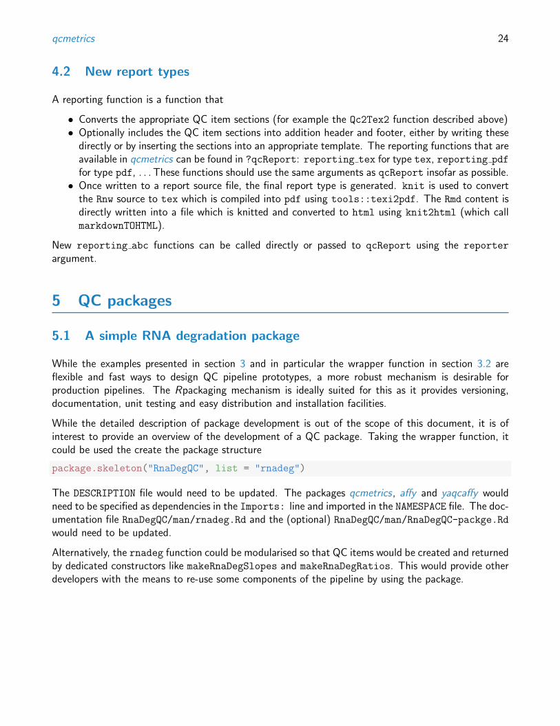
4.2 New report types

A reporting function is a function that

• Converts the appropriate QC item sections (for example the Qc2Tex2 function described above)• Optionally includes the QC item sections into addition header and footer, either by writing these

directly or by inserting the sections into an appropriate template. The reporting functions that areavailable in qcmetrics can be found in ?qcReport: reporting tex for type tex, reporting pdf

for type pdf, . . . These functions should use the same arguments as qcReport insofar as possible.• Once written to a report source file, the final report type is generated. knit is used to convert

the Rnw source to tex which is compiled into pdf using tools::texi2pdf. The Rmd content isdirectly written into a file which is knitted and converted to html using knit2html (which callmarkdownTOHTML).

New reporting abc functions can be called directly or passed to qcReport using the reporter

argument.

5 QC packages

5.1 A simple RNA degradation package

While the examples presented in section 3 and in particular the wrapper function in section 3.2 areflexible and fast ways to design QC pipeline prototypes, a more robust mechanism is desirable forproduction pipelines. The Rpackaging mechanism is ideally suited for this as it provides versioning,documentation, unit testing and easy distribution and installation facilities.

While the detailed description of package development is out of the scope of this document, it is ofinterest to provide an overview of the development of a QC package. Taking the wrapper function, itcould be used the create the package structure

package.skeleton("RnaDegQC", list = "rnadeg")

The DESCRIPTION file would need to be updated. The packages qcmetrics, affy and yaqcaffy wouldneed to be specified as dependencies in the Imports: line and imported in the NAMESPACE file. The doc-umentation file RnaDegQC/man/rnadeg.Rd and the (optional) RnaDegQC/man/RnaDegQC-packge.Rdwould need to be updated.

Alternatively, the rnadeg function could be modularised so that QC items would be created and returnedby dedicated constructors like makeRnaDegSlopes and makeRnaDegRatios. This would provide otherdevelopers with the means to re-use some components of the pipeline by using the package.

qcmetrics 25

5.2 A QC pipeline repository

The wiki on the qcmetrics github page5 can be edited by any github user and will be used to cite,document and share QC functions, pipelines and packages, in particular those that make use of theqcmetrics infrastructure.

6 Conclusions

Rand Bioconductor are well suited for the analysis of high throughput biology data. They provide firstclass statistical routines, excellent graph capabilities and an interface of choice to import and manipulatevarious omics data, as demonstrated by the wealth of packages6 that provide functionalities for QC.

The qcmetrics package is different than existing Rpackages and QC systems in general. It proposes aunique domain-independent framework to design QC pipelines and is thus suited for any use case. Theexamples presented in this document illustrated the application of qcmetrics on data containing singleor multiple samples or experimental runs from different technologies. It is also possible to automate thegeneration of QC metrics for a set of repeated (and growing) analyses of standard samples to establishlab memory types of QC reports, that track a set of metrics for controlled standard samples over time.It can be applied to raw data or processed data and tailored to suite precise needs. The popularisationof integrative approaches that combine multiple types of data in novel ways stresses out the need forflexible QC development.

qcmetrics is a versatile software that allows rapid and easy QC pipeline prototyping and developmentand supports straightforward migration to production level systems through its well defined packagingmechanism.

5https://github.com/lgatto/qcmetrics6http://bioconductor.org/packages/release/BiocViews.html# QualityControl

qcmetrics 26

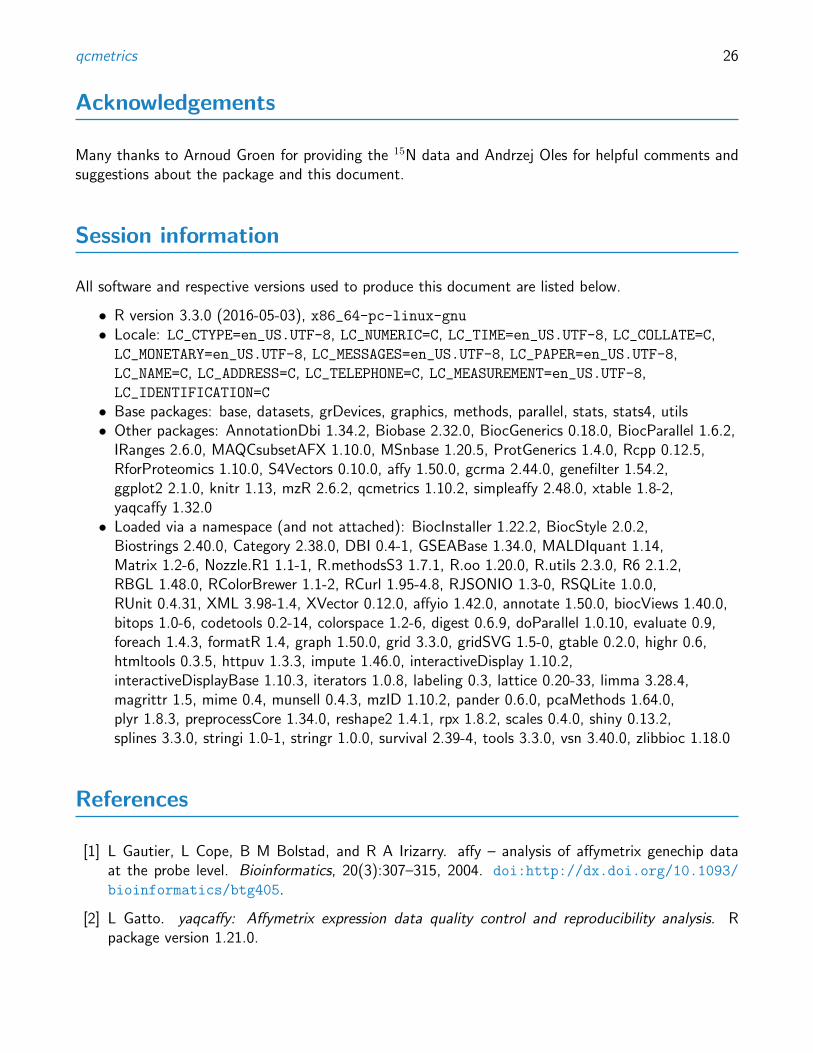
Acknowledgements

Many thanks to Arnoud Groen for providing the 15N data and Andrzej Oles for helpful comments andsuggestions about the package and this document.

Session information

All software and respective versions used to produce this document are listed below.

• R version 3.3.0 (2016-05-03), x86_64-pc-linux-gnu• Locale: LC_CTYPE=en_US.UTF-8, LC_NUMERIC=C, LC_TIME=en_US.UTF-8, LC_COLLATE=C,LC_MONETARY=en_US.UTF-8, LC_MESSAGES=en_US.UTF-8, LC_PAPER=en_US.UTF-8,LC_NAME=C, LC_ADDRESS=C, LC_TELEPHONE=C, LC_MEASUREMENT=en_US.UTF-8,LC_IDENTIFICATION=C

• Base packages: base, datasets, grDevices, graphics, methods, parallel, stats, stats4, utils• Other packages: AnnotationDbi 1.34.2, Biobase 2.32.0, BiocGenerics 0.18.0, BiocParallel 1.6.2,

IRanges 2.6.0, MAQCsubsetAFX 1.10.0, MSnbase 1.20.5, ProtGenerics 1.4.0, Rcpp 0.12.5,RforProteomics 1.10.0, S4Vectors 0.10.0, affy 1.50.0, gcrma 2.44.0, genefilter 1.54.2,ggplot2 2.1.0, knitr 1.13, mzR 2.6.2, qcmetrics 1.10.2, simpleaffy 2.48.0, xtable 1.8-2,yaqcaffy 1.32.0• Loaded via a namespace (and not attached): BiocInstaller 1.22.2, BiocStyle 2.0.2,

Biostrings 2.40.0, Category 2.38.0, DBI 0.4-1, GSEABase 1.34.0, MALDIquant 1.14,Matrix 1.2-6, Nozzle.R1 1.1-1, R.methodsS3 1.7.1, R.oo 1.20.0, R.utils 2.3.0, R6 2.1.2,RBGL 1.48.0, RColorBrewer 1.1-2, RCurl 1.95-4.8, RJSONIO 1.3-0, RSQLite 1.0.0,RUnit 0.4.31, XML 3.98-1.4, XVector 0.12.0, affyio 1.42.0, annotate 1.50.0, biocViews 1.40.0,bitops 1.0-6, codetools 0.2-14, colorspace 1.2-6, digest 0.6.9, doParallel 1.0.10, evaluate 0.9,foreach 1.4.3, formatR 1.4, graph 1.50.0, grid 3.3.0, gridSVG 1.5-0, gtable 0.2.0, highr 0.6,htmltools 0.3.5, httpuv 1.3.3, impute 1.46.0, interactiveDisplay 1.10.2,interactiveDisplayBase 1.10.3, iterators 1.0.8, labeling 0.3, lattice 0.20-33, limma 3.28.4,magrittr 1.5, mime 0.4, munsell 0.4.3, mzID 1.10.2, pander 0.6.0, pcaMethods 1.64.0,plyr 1.8.3, preprocessCore 1.34.0, reshape2 1.4.1, rpx 1.8.2, scales 0.4.0, shiny 0.13.2,splines 3.3.0, stringi 1.0-1, stringr 1.0.0, survival 2.39-4, tools 3.3.0, vsn 3.40.0, zlibbioc 1.18.0

References

[1] L Gautier, L Cope, B M Bolstad, and R A Irizarry. affy – analysis of affymetrix genechip dataat the probe level. Bioinformatics, 20(3):307–315, 2004. doi:http://dx.doi.org/10.1093/

bioinformatics/btg405.

[2] L Gatto. yaqcaffy: Affymetrix expression data quality control and reproducibility analysis. Rpackage version 1.21.0.

qcmetrics 27

[3] P G A Pedrioli et al. A common open representation of mass spectrometry data and its applicationto proteomics research. Nat. Biotechnol., 22(11):1459–66, 2004. doi:10.1038/nbt1031.

[4] L Gatto and K S Lilley. MSnbase – an R/Bioconductor package for isobaric tagged mass spec-trometry data visualization, processing and quantitation. Bioinformatics, 28(2):288–9, Jan 2012.doi:10.1093/bioinformatics/btr645.

[5] K M Foster, S Degroeve, L Gatto, M Visser, R Wang, K Griss, R Apweiler, and L Martens.A posteriori quality control for the curation and reuse of public proteomics data. Proteomics,11(11):2182–94, 2011. doi:10.1002/pmic.201000602.

[6] J Krijgsveld, R F Ketting, T Mahmoudi, J Johansen, M Artal-Sanz, C P Verrijzer, R H Plasterk,and A J Heck. Metabolic labeling of c. elegans and d. melanogaster for quantitative proteomics.Nat Biotechnol, 21(8):927–31, Aug 2003. doi:10.1038/nbt848.

[7] A Groen, L Thomas, K Lilley, and C Marondedze. Identification and quantitation of signalmolecule-dependent protein phosphorylation. Methods Mol Biol, 1016:121–37, 2013. doi:

10.1007/978-1-62703-441-8_9.

[8] Y Xie. Dynamic Documents with R and knitr. Chapman and Hall/CRC, 2013. ISBN 978-1482203530. URL: http://yihui.name/knitr/.

[9] JJ Allaire, J Horner, V Marti, and N Porte. markdown: Markdown rendering for R, 2013. Rpackage version 0.6.3. URL: http://CRAN.R-project.org/package=markdown.

[10] N Gehlenborg. Nozzle.R1: Nozzle Reports, 2013. R package version 1.1-1. URL: http://CRAN.R-project.org/package=Nozzle.R1.