Embed Size (px)
Citation preview

Ramanujan J (2012) 28:443–461DOI 10.1007/s11139-012-9412-8
The q-cosine Fourier transform and the q-heat equation
Ahmed Fitouhi · Fethi Bouzeffour
Received: 31 January 2000 / Accepted: 16 February 2001 / Published online: 13 July 2012© The Author(s) 2012. This article is published with open access at Springerlink.com
Abstract The aim of this work is to establish in great detail The q-Fourier analysisrelated to the q-cosine. The wise reader will note that the considered q-cosine co-incides with the one given by T.H. Koornwinder and S.F. Swarttouw. Through theq-cosine product formula, we define and analyze the properties of the q-even transla-tion and the q-convolution. Adopting the Titchmarsh approach, we study the q-cosineFourier transform and its inverse formula.
The second theme of this paper is an application of the q-Fourier analysis devel-oped earlier. We extend the heat representation theory inaugurated by P.C. Rosen-bloom and D.V. Widder to the q-analogue. We construct the q-solution source, theq-heat polynomials and solve the q-analytic Cauchy problem.
Keywords Basic orthogonal polynomials and functions · Basic hypergeometricintegrals
Mathematics Subject Classification (2000) Primary 33D45 · Secondary 33D6043
This research is supported by NPST Program of King Saud University, project number10-MAT1293-02.
EDITORIAL NOTE: The article was accepted on 16 February, 2001, before the papers of theRamanujan Journal were handled electronically. Unfortunately this article in its printed form wasmisplaced. The delay caused in publication is regretted.
A. Fitouhi (�)Department of Mathematics, Faculty of Sciences of Tunis University El-Manar, 1060 Tunis, Tunisiae-mail: [email protected]
F. BouzeffourDepartment of Mathematics, College of Sciences, King Saud University, P.O. Box 2455, Riyadh11451, Saudi Arabiae-mail: [email protected]
444 A. Fitouhi, F. Bouzeffour
1 Introduction
During the last years, an intensive work was founded about the so-called q-basictheory. Taking account of the well-known Ramanujan works shown at the beginningof this century by Jackson ([9, 10]), many authors such as Askey, Gasper, Ismail,Rogers, Andrew, Koornwinder, and others (see references) have recently developedthis topic.
The present article is devoted to the study of the q-analogue of the Fourier trans-forms and to showing how it plays a central role in solving the q-heat equation asso-ciated to the second q-derivative operator. The method used here differs from thosegiven by T.H. Koornwinder and R.F. Swarttouw, who discovered a q-analogue ofHankel’s Fourier–Bessel via some q-analogue orthogonality relations. We note thatPh. Feinsilver [4] gave a q-Harmonic Analysis for a q-Laplace transform with inver-sion formula.
Without entering into a dilemma through the analysis presented here, it seems thatthe point of view of T.H. Koornwinder and R.F. Swarttouw [12] is more suitable forharmonic analysis. We take as definition of the q-cosine the one given by the previousauthors with a simple change and we prefer to write it as a series of functions denotedas bn(x;q2). This q-cosine appears as an eigenfunction of the operator Δq . Owingto a nice paper [12], we give a product formula written with the q-Jackson integraland we study the q-translation and the q-convolution. Next we define the q-analogueof the cosine Fourier transform with the purpose to find the transformation inverse.To this end, we prove the equivalent of the so-called Riemann–Lebesgue Lemma anddiscover that the Titchmarsh approach holds [15].
A motivation behind this work is to state some result about the q-heat equation as-sociated to Δq operator. We attempt to extend the heat representation theory studiedin many cases ([5, 7, 14], etc.). We define the q-heat polynomials and find that theyare linked to the q-Hermite polynomials [13] and constitute with the q-associatedfunctions a biorthogonal system. We conclude by solving the q-analytic Cauchy prob-lem related to the q-heat equation.
2 Notations and preliminaries
We begin by recalling some q-elements of quantum analysis adapting the notationused in the book of Gasper and Rahman [6]. Let a and q be real numbers such that0 < q < 1, the q-shift factorial is defined by
(a;q)0 = 1, (a;q)n =n−1∏
k=0
(1 − aqk
), n = 1,2, . . . ,∞. (1)
A basic hypergeometric series is
rϕs(a1, . . . , ar ;b1, . . . , bs;q, z) =∞∑
k=0
(a1, . . . , ar ;q)k
(b1, . . . , bs, q;q)k
[(−1)kq(k
2)]1+s−r
zk.

The q-cosine Fourier transform and the q-heat equation 445
A function f is q-regular at zero if limn→∞ f (xqn) = f (0) exists and is independentof x.
The q-derivative Dqf of a function f is defined by
Dqf (x) = f (x) − f (qx)
(1 − q)x, x �= 0. (2)
The q-derivative at zero is defined by
Dqf (0) = limn→∞
f (xqn) − f (0)
xqn,
if it exists and does not depend on x.We introduce the set
Rq = {qk; k ∈ Z
}.
The q-integral of Jackson is defined by
∫ a
0f (x)dqx = (1 − q)a
∞∑
k=0
f(aqk
)qk,
∫ ∞
0f (x)dqx = (1 − q)
∞∑
k=−∞f
(qk
)qk.
The q-integration by parts is given for suitable functions f and g by∫ ∞
0f (x)Dqg(x) dqx = [
f (x)g(x)]∞
0 −∫ ∞
0f (x)Dqg
(q−1x
)dqx. (3)
The q-analogue of the Gamma function is defined as
Γq(x) = (q;q)∞(qx;q)∞
(1 − q)1−x, (4)
which tends to Γ (x) when q tends to 1−.
3 q-Trigonometric functions
We define the q-cosine as
cos(x;q2) = 1φ1
(0;q;q2, (1 − q)2x2) =
∞∑
n=0
(−1)nbn
(x;q2), (5)
where we have put
bn
(x;q2) = bn
(1;q2)x2n = qn(n−1) (1 − q)2n
(q;q)2n
x2n. (6)

446 A. Fitouhi, F. Bouzeffour
In the same way, the q-sine is given by
sin(x;q2) = (1 − q)x1φ1
(0;q3;q2, (1 − q)2x2) =
∞∑
n=0
(−1)ncn
(x;q2),
with
cn
(x;q2) = cn
(1;q2)x2n+1 = qn(n−1)(1 − q)2n+1
(q;q)2n+1x2n+1.
These q-trigonometric functions differ and should not be confused with the functionscosq and sinq considered in [6, p. 23]; but coincide with the one given in [12] and[15] with a minor change of variable. Furthermore, we have
Proposition 3.1 The following statements hold:
1.
bn
(0, q2) = δn,0, Δqbn
(x;q2) = bn−1
(x;q2), n ≥ 1;
2.
∣∣bn
(x;q2)∣∣ ≤ x2n
(2n)! ,
where
Δqu(x) = (D2
qu)(
q−1x). (7)
Proof We only prove Part 2 since Part 1 is deduced from the definition of Δq .The coefficients bn(1;q2), defined by (6), can be written as
bn
(1;q2) =
n−1∏
j=0
qj − qj+1
1 − q2j+1
qj − qj+1
1 − q2j+2
=n−1∏
j=0
e−j t − e−(j+1)t
1 − e−(2j+1)t.e−j t − e−(j+1)t
1 − e−(2j+2)t,
where we have put q = e−t , t > 0.Since the functions
f (t) = e−j t − e−(j+1)t
1 − e−(j+1)tand g(t) = e−j t − e−(j+1)t
1 − e−(2j+2)t,
decrease on ]0,∞[, we obtain
bn
(1;q2) ≤ 1
(2n)! . �

The q-cosine Fourier transform and the q-heat equation 447
As a consequence of the previous proposition, we can show that for λ ∈ C thefunction
cos(λx;q2) =
∞∑
0
(−1)nbn
(x;q2)λ2n,
is the unique analytic solution of the q-differential equation
Δqu(x) = −λ2u(x), (8)
with
u(0, q) = 1, (Dqu)(0) = 0. (9)
Proposition 3.2 For x ∈ Rq and Log(1−q)Log(q)
∈ Z, we have
1.∣∣cos
(x, q2)∣∣ ≤ 1
(q;q2)2∞;
2.
limx→∞ cos
(x, q2) = 0;
3.∣∣sin
(x, q2)∣∣ ≤ 1
(q;q2)2∞;
4.
limx→∞ sin
(x, q2) = 0.
Proof To prove Parts 1 and 2, we use the properties of 1φ1 given in [12] and theirconnection to the q-cosine. We obtain
∣∣cos(q1+n;q2)∣∣ ≤ 1
(q;q2)2∞
{1 if n ≥ 0,
qn2if n ≤ 0.
(10)
hence Parts 1 and 2 follow. A similar argument shows Parts 3 and 4. �
Now we try to find a product formula for the q-cosine functions. We begin byproving the following result.
Proposition 3.3 For reals x and y, y �= 0, we have
cos(x, q2) cos
(y, q2)
=∞∑
k=0
qk
(x
y
)2k s=k∑
s=−k
(−1)k−s q(k−s2 )
(q;q)k−s(q;q)k+s
cos(qsy, q2). (11)
Note that this formula can be expressed in terms of 1ϕ1 as follows
448 A. Fitouhi, F. Bouzeffour
cos(x, q2) cos
(y, q2) =
∞∑
s=−∞qs
(x
y
)2s(q1+2s;q)∞
(q;q)∞
×1 ϕ1
(0;q1+2s;q2, q
x2
y2
)cos
(qsy, q2). (12)
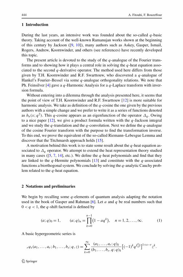
Proof To show (11) and (12), we begin by expanding the q-cosines in series abso-lutely and uniformly convergent on every compact of R. From the product rule ofseries and the fact that
1
(q;q)2n−2k
= (q2n−2k+1, q)∞(q;q)∞
= 0, k > n,
we obtain for y �= 0
cos(x;q2) cos
(y;q2) =
∞∑
k=0
q2k2
(q;q)2k
(x
y
)2k ∞∑
n=0
(−1)nqn2−n
(q;q)2n−2k
q−2nky2n.
On the other hand, we have
1
(q;q)2n−2k
= q−k(2k−1)+2nk
(q;q)2n
s=k∑
s=−k
(−1)k−s q(k−s2 )
(q;q)k−s(q;q)k+s
q2ns .
We deduce (11) after the interchange of summation order. To prove (12), we write
cos(x;q2) cos
(y;q2) = I + J,
with
I =∞∑
s=0
cos(qsy;q2)∑
k≥s
qk
(x
y
)2k(−1)k−sq
(k−s)(k−s−1)2
(q;q)k+s(q;q)k−s
,
J =−1∑
s=−∞cos
(qsy;q2) ∑
k≥−s
qk
(x
y
)2k(−1)k−sq
(k−s)(k−s−1)2
(q;q)k−s(q;q)k+s
.
In I , we make the change k − s into k and use the equality
(q;q)k+2s = (q;q)2s
(q1+2s;q)
k,
to obtain
I =∞∑
s=0
qs
(x
y
)2s(q2s+1;q)∞
(q;q)∞1φ1
(0;q1+2s;q, q
(q2/y2)) cos
(qsy;q2).
Now we make the change k + s into k in J and use the equalities
(q;q)k−2s = (q;q)−2s
(q1−2s;q)
k, −s ≥ 1,

The q-cosine Fourier transform and the q-heat equation 449
(k − 2s)(k − 2s − 1)
2= (k − 2)(k − 3)
2− 2sk + 2s2 − 1,
and
(q1−2s;q)
∞1φ1(0;q1−2s;q, q1−2sx2/y2)
= qs(2s−1)q1−2s(x2/y2)2s(
q1+2s;q)∞ 1φ1
(0;q1+2s;q, qx2/y2).
This identity is easily deduced from [11]. Then we obtain
J =−1∑
s=−∞qs
(x2/y2)2s (q1+2s;q)∞
(q;q)∞1φ1
(0;q1+2s;q, qx2/y2) cos
(qsy;q2).
We add these sums to find that (12) holds. �
Remark 3.4 (1) If we replace y by qy , x by qx , and assume the proposition thehypothesis, we obtain from (12) that the following integral representation holds
cos(qx;q2) cos
(qy;q2)
= (q2(x−y)+1;q)∞(q;q)∞
∫ ∞
0u2(x−y)
1φ1(0;u2(x−y)+1;q, qu2) cos
(qyu;q2)dqu.
(2) The product formula (11) leads to
cos(x;q2) cos
(y;q2) =
∞∑
n=0
bn
(x;q2)Δn
q cos(y;q2). (13)
4 q-Translation and q-convolution
We define, for x and y in Rq , the measure
dqμ(x,y) =∞∑
s=−∞D
(x, y;qs
)qsδyqs , (14)
where δu denotes the unit mass supported at u, and
D(x, y;qs
) =(
x
y
)2s (q( xy)2;q)∞
(q;q)∞1φ1
(0;q
(x
y
)2
;q, q1+2s
). (15)
Proposition 4.1 (1) For x and y in Rq , we have
dqμ(x,y) = dqμ(y,x).
(2) dqμ(x,y) is of bounded variation.
450 A. Fitouhi, F. Bouzeffour
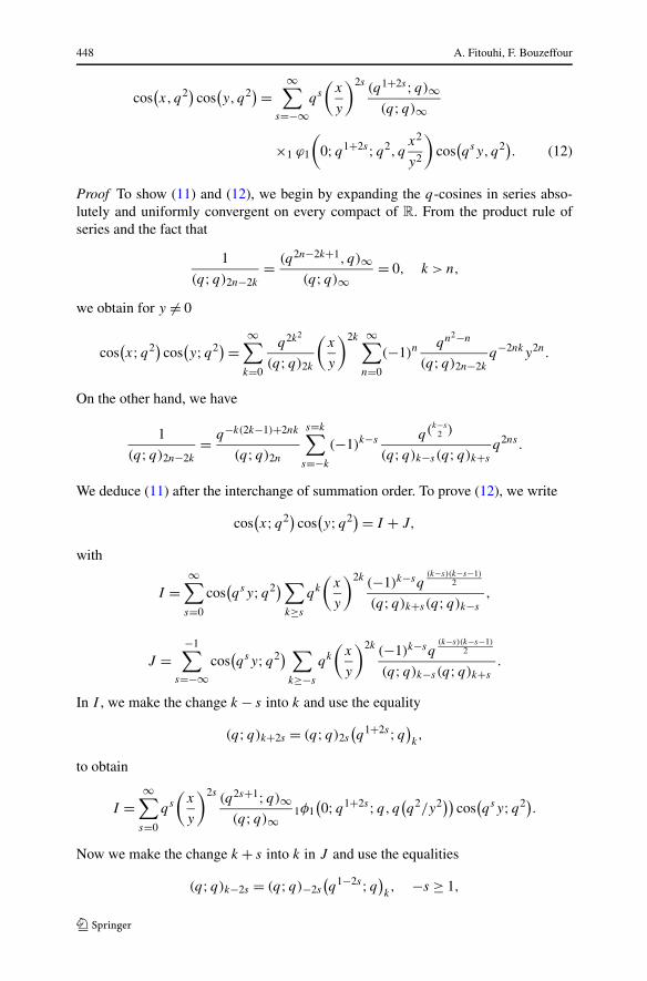
(3)∫
dqμ(x,y)(t) = 1.
Proof For n,m ∈ Z, the relation (2.3) from [12] leads to
D(qn, qm;qs
) = D(qm,qn;qs+m−n
).
We obtain Part 1 after the change s − n + m by s.To prove Part 2, we suppose | x
y| ≤ 1; from the formulas (2.4) in [12] we have
|dqμ(x,y)|var ≤( |y|2 + q|x|2
|y|2 − q|x|2)
(q| xy|2;−q, q)∞(q, q)∞
. (16)
Finally, from (2.8) in [12], we can show that Part 3 is true. �
We introduce the q-translation which generalizes the even translation given by12 (δx+y + δx−y).
Let f be a function with support in Rq , the q-translation is defined for x and y inRq by
Tx,qf (y) =∫ ∞
0f (t) dqμ(x,y)(t). (17)
From the previous proposition and the q-product formula (12), we have
Proposition 4.2 Let f be a function with compact support in Rq . We have
(i)
Tq,y cos(x;q2) = cos
(x;q2) cos
(y;q2).
(ii)
Tq,yf (x) = Tq,xf (y),
Tq,0f = f.
(iii)
ΔqTq,yf = Tq,yΔqf,
Δq,;yTq,yf = Tq,yΔq,yf.
(iv) The function u(x, y) = Tq,yf (x) is a solution of the problem
Δq,xu(x, y) = Δq,yu(x, y),
u(x,0) = f (x).

The q-cosine Fourier transform and the q-heat equation 451
From the relation
Δnq(f )(x) = q(2−n)n(q;q)2n
(1 − q)2n
n∑
k=−n
(−1)n−k q(n−k2 )
(q;q)n−k(q;q)n+k
f(qkx
),
we can write the q-translation of a function f as
Tq,yf (x) =∞∑
n=0
bn
(y, q2)Δn
q,xf (x), (18)
and have in the limit when q tends to 1− the classical even translation cited before.Now we denote by L1
q(Rq) the space of functions f defined on Rq such that
‖f ‖1,q =∫ ∞
−∞∣∣f (t)
∣∣dqt < ∞.
Then we are able to define the q-convolution by
f �q g(x) = (1 + q−1)1/2
Γq2(1/2)
∫ ∞
0Tx,qf (y)g(y) dqy, (19)
where f and g are two functions in L1q(Rq). We can show that this space is an algebra.
5 q-Analogue of Fourier-cosine
In this section, we suppose Log(1−q)Log(q)
∈ Z. The q-analogue of Fourier transform isdefined for λ ∈ Rq by
F (f )(λ) = (1 + q−1)1/2
Γq2(1/2)
∫ ∞
0f (t) cos
(λt;q2)dqt, (20)
where f is a function in L1q(Rq).
This definition is the same (after a minor change) as that given by T.H. Koorn-winder and R.F. Swarttouw (see [12]).
Proposition 5.1 For f,g ∈ L1q(Rq), the following properties hold:
(1)
∣∣Fq(f )(λ)∣∣ ≤ 1
[q(1 − q)] 12 (q;q)∞
‖f ‖1,q , λ ∈ Rq; (21)
(2)
Fq(Tq,xf )(λ) = cos(λx;q2)Fq(f )(λ), λ ∈ Rq; (22)

452 A. Fitouhi, F. Bouzeffour
(3)
Fq(f �q g) = Fq(f )Fq(g).
Proof Part 1. The inequality (21) follows from Proposition 3.2 and the identity(q;q2)
∞(q2;q2)
∞ = (q;q)∞.
Part 2 is a direct consequence of the q-product formula (12).Part 3 is obtained after the exchange of the integration order and taking into ac-
count the invariability of the q-integral by the q-translation. �
Now we focus our attention on the inversion of the linear map Fq . We proceedby looking at the q-analogue of the Riemman–Lebesgue Lemma, the localizationtheorem, and we show that the Titchmarsh approach holds in the q-theory.
Proposition 5.2 Let f be a function in L1q(Rq), then
limλ−→∞ Fq(f )(λ) = 0, λ ∈ Rq .
Proof To prove this, first we have from Proposition 3.2
∣∣f (x) cos(λx;q2)∣∣ ≤ 1
(q;q2)2∞
∣∣f (x)∣∣ ∈ L1
q(Rq), x,λ ∈ Rq .
And for λ ∈ Rq we have
limλ→∞f (x) cos
(λx;q2) = 0, λ ∈ Rq,
so the result is true. �
Proposition 5.3 We have the identity
∫ ∞
0
sin(x;q2)
xdqx =
Γ 2q2(
12 )
1 + q−1.
Proof This is a consequence of (2.8) in [12]. �
Proposition 5.4 Let f : (0,∞) → C satisfy the conditions:
(1) f ∈ L1q(Rq),
(2) For a ∈ Rq , there exists C(a) > 0 such that
∣∣f(aqk
) − f (0)∣∣ ≤ C(a)qk, k = 0,1,2, . . . .
Then
limλ→+∞
∫ ∞
0f (x)
sin(λx;q2)
xdqx =
Γ 2q2(
12 )
1 + q−1f (0).
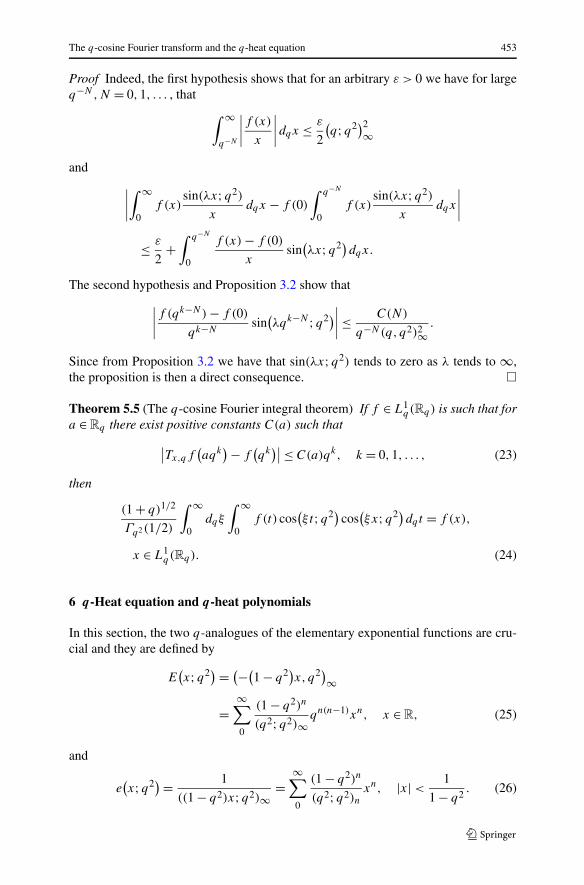
The q-cosine Fourier transform and the q-heat equation 453
Proof Indeed, the first hypothesis shows that for an arbitrary ε > 0 we have for largeq−N,N = 0,1, . . . , that
∫ ∞
q−N
∣∣∣∣f (x)
x
∣∣∣∣dqx ≤ ε
2
(q;q2)2
∞
and∣∣∣∣∫ ∞
0f (x)
sin(λx;q2)
xdqx − f (0)
∫ q−N
0f (x)
sin(λx;q2)
xdqx
∣∣∣∣
≤ ε
2+
∫ q−N
0
f (x) − f (0)
xsin
(λx;q2)dqx.
The second hypothesis and Proposition 3.2 show that
∣∣∣∣f (qk−N) − f (0)
qk−Nsin
(λqk−N ;q2)
∣∣∣∣ ≤ C(N)
q−N(q, q2)2∞.
Since from Proposition 3.2 we have that sin(λx;q2) tends to zero as λ tends to ∞,the proposition is then a direct consequence. �
Theorem 5.5 (The q-cosine Fourier integral theorem) If f ∈ L1q(Rq) is such that for
a ∈ Rq there exist positive constants C(a) such that
∣∣Tx,qf(aqk
) − f(qk
)∣∣ ≤ C(a)qk, k = 0,1, . . . , (23)
then
(1 + q)1/2
Γq2(1/2)
∫ ∞
0dqξ
∫ ∞
0f (t) cos
(ξ t;q2) cos
(ξx;q2)dqt = f (x),
x ∈ L1q(Rq). (24)
6 q-Heat equation and q-heat polynomials
In this section, the two q-analogues of the elementary exponential functions are cru-cial and they are defined by
E(x;q2) = (−(
1 − q2)x, q2)∞
=∞∑
0
(1 − q2)n
(q2;q2)∞qn(n−1)xn, x ∈ R, (25)
and
e(x;q2) = 1
((1 − q2)x;q2)∞=
∞∑
0
(1 − q2)n
(q2;q2)nxn, |x| < 1
1 − q2. (26)

454 A. Fitouhi, F. Bouzeffour
These functions satisfy the identity
e(x;q2)E
(−x;q2) = 1,
and have as limit, when q tends to 1−, the classical exponential function.Now we purpose to give the q-analogue of the heat equation associated to the
second derivative operator (even in x)
δ2u
δx2= δu
δt, x ∈ R, t > 0. (27)
We consider as q-heat equation associated to the second q-derivative operator thepartial q-difference equation
(Δq,xu)(x, t) = (Dq2,t u)(x, t). (28)
We take as the initial condition
u(x,0) = f (x), f ∈ L1q(Rq). (29)
6.1 q-Solution source
To find the solution source related to the q-heat equation, we apply the Fouriermethod with the adapted q-Fourier cosine studied before.
Putting
U(λ, t) = F(u(x, t)
)(λ),
Eq. (28) becomes
Dq2,tU(λ, qt) = −λ2U(λ, t),
and, taking into account conditions (29), we obtain
U(λ, t) = F (f )(λ)e(−λ2t;q2).
The problem consists in finding the function which has e(−λ2t;q2) as its q-Fourier-cosine transform. For this end, we need the following lemma.
Lemma 6.1 For n = 0,1,2, . . . and t > 0, we have∫ ∞
0e
(− λ2
qt (1 + q)2, q2
)bn
(λ;q2)dqλ
= (1 − q)(q2,− 1+q
1−qq2t,− 1−q
1+q1t, q2)∞
(q,− 1−q1+q
1qt
,− 1+q1−q
q3t;q2)∞(1 − q2)n
(q2, q2)ntn.
Proof From (26) we find
∫ ∞
0e
(− λ2
qt (1 + q)2, q2
)λ2n dqλ = (1 − q)
∞∑
−∞
q(2n+1)k
(− 1−q1+q
q2k
qt, q2)∞
.
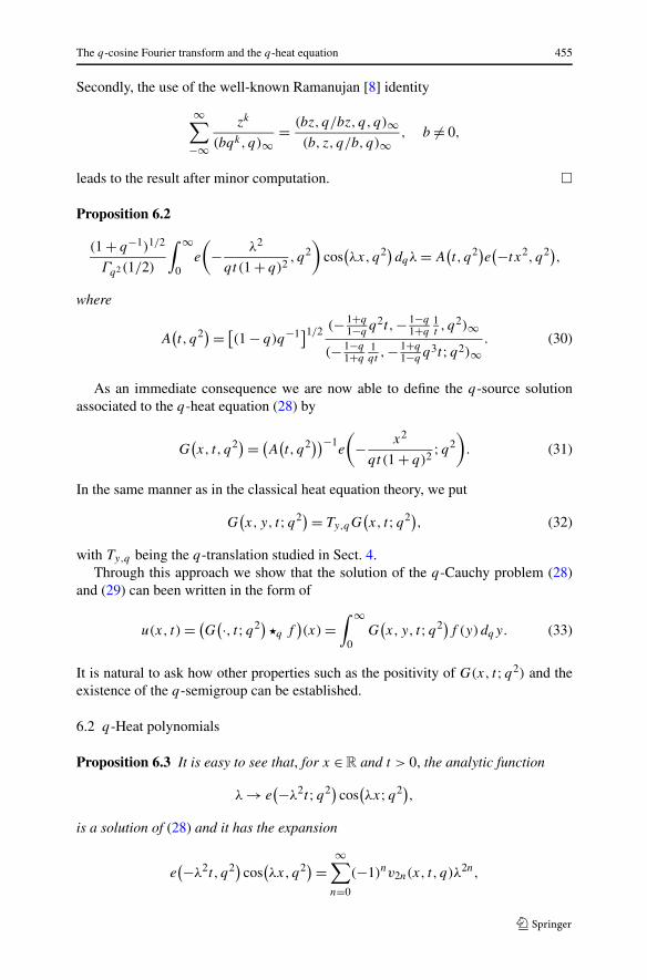
The q-cosine Fourier transform and the q-heat equation 455
Secondly, the use of the well-known Ramanujan [8] identity
∞∑
−∞
zk
(bqk, q)∞= (bz, q/bz, q, q)∞
(b, z, q/b, q)∞, b �= 0,
leads to the result after minor computation. �
Proposition 6.2
(1 + q−1)1/2
Γq2(1/2)
∫ ∞
0e
(− λ2
qt (1 + q)2, q2
)cos
(λx,q2)dqλ = A
(t, q2)e
(−tx2, q2),
where
A(t, q2) = [
(1 − q)q−1]1/2 (− 1+q1−q
q2t,− 1−q1+q
1t, q2)∞
(− 1−q1+q
1qt
,− 1+q1−q
q3t;q2)∞. (30)
As an immediate consequence we are now able to define the q-source solutionassociated to the q-heat equation (28) by
G(x, t, q2) = (
A(t, q2))−1
e
(− x2
qt (1 + q)2;q2
). (31)
In the same manner as in the classical heat equation theory, we put
G(x, y, t;q2) = Ty,qG
(x, t;q2), (32)
with Ty,q being the q-translation studied in Sect. 4.Through this approach we show that the solution of the q-Cauchy problem (28)
and (29) can been written in the form of
u(x, t) = (G
(·, t;q2) �q f)(x) =
∫ ∞
0G
(x, y, t;q2)f (y)dqy. (33)
It is natural to ask how other properties such as the positivity of G(x, t;q2) and theexistence of the q-semigroup can be established.
6.2 q-Heat polynomials
Proposition 6.3 It is easy to see that, for x ∈ R and t > 0, the analytic function
λ → e(−λ2t;q2) cos
(λx;q2),
is a solution of (28) and it has the expansion
e(−λ2t, q2) cos
(λx,q2) =
∞∑
n=0
(−1)nv2n(x, t, q)λ2n,
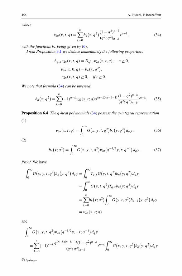
456 A. Fitouhi, F. Bouzeffour
where
v2n(x, t, q) =n∑
k=0
bk
(x, q2) (1 − q2)n−k
(q2;q2)n−k
tn−k, (34)
with the functions bn being given by (6).From Proposition 3.1 we deduce immediately the following properties:
Δq,xv2n(x, t, q) = Dq2,t v2n(x, t, q), n ≥ 0,
v2n(x,0, q) = bn
(x, q2),
v2n(x, t, q) ≥ 0, if t ≥ 0.
We note that formula (34) can be inverted:
bn
(x;q2) =
n∑
k=0
(−1)n−kv2k(x, t;q)q(n−k)(n−k−1) (1 − q2)n−k
(q2;q2)n−k
tn−k. (35)
Proposition 6.4 The q-heat polynomials (34) possess the q-integral representation
(1)
v2n(x, t;q) =∫ ∞
0G
(x, y, t, q2)bn
(y;q2)dqy. (36)
(2)
bn
(x;q2) =
∫ ∞
0G
(x, y, t, q2)v2n
(q−1/2y, t;q−1)dqy. (37)
Proof We have
∫ ∞
0G
(x, y, t, q2)bn
(y;q2)dqy =
∫ ∞
0Tq,xG
(y, t, q2)bn
(y;q2)dqy
=∫ ∞
0G
(y, t, q2)Tq,xbn
(y;q2)dqy
=n∑
k=0
bk
(x;q2)
∫ ∞
0G
(y, t, q2)bn−k
(y;q2)dqy
= v2n(x, t;q)
and∫ ∞
0G
(x, y, t, q2)v2n
(q−1/2y,−t;q−1)dqy
=n∑
k=0
(−1)n−k q(n−k)(n−k−1)(1 − q2)n−k
(q2;q2)n−k
tn−k
∫ ∞
0G
(x, y, t, q2)bk
(y, q2)dqy

The q-cosine Fourier transform and the q-heat equation 457
=n∑
k=0
(−1)n−kq(n−k)(n−k−1) (1 − q2)n−k
(q2;q2)n−k
tn−kv2k(x, t;q)
= bn
(x;q2). �
In [14], the authors defined the so-called associated functions by the Appell trans-form. We extend this notion by defining for t > 0 the q-associated functions of v2n
by
w2n(x, t;q) = (−1)nΔnq,yG
(x, y, t;q2)∣∣
y=0. (38)
It is easy to see that
w2n(x, t;q) = (1 + q−1)1/2
Γq2(1/2)
∫ ∞
0e(−tλ2, q2)λ2n cos
(λx,q2)dqλ. (39)
Proposition 6.5 (Biorthogonality) For t > 0 and n,m ∈ N, we have
∫ ∞
0w2m(x, t;q)v2n
(q1/2x,−t;q)
dqx = (−1)mδn,m.
Proof By (37), we have
Δmq bn
(x;q2) =
∫ ∞
0Δm
q G(x, y, t, q2)v2n
(q−1/2y, t;q−1)dqy.
Putting x = 0, we obtain
∫ ∞
0w2m(y, t;q)v2n
(q−1/2y, t;q−1)dqy = (−1)mδn,m.
�
6.3 Convergence of∑
n≥0 αnv2n(x, t;q)
Now we establish the following estimates that will be needed later
Lemma 6.6 For n = 0,1, . . . and 0 <x2
0t0
< +∞, we have
∣∣v2n(x0, t0, q)∣∣ ≥ (1 − q2)n
(q2;q2)n|t0|n ≥ |t0|n
n! .
Proof Indeed, the first inequality is a consequence of b0(1;q2) = 1 and the hypothe-sis, and the second follows from
1
n! ≤ (1 − q2)n
(q2;q2)n. �
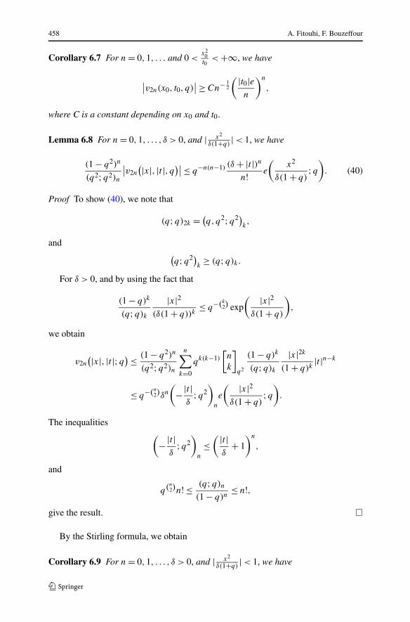
458 A. Fitouhi, F. Bouzeffour
Corollary 6.7 For n = 0,1, . . . and 0 <x2
0t0
< +∞, we have
∣∣v2n(x0, t0, q)∣∣ ≥ Cn− 1
2
( |t0|en
)n
,
where C is a constant depending on x0 and t0.
Lemma 6.8 For n = 0,1, . . . , δ > 0, and | x2
δ(1+q)| < 1, we have
(1 − q2)n
(q2;q2)n
∣∣v2n
(|x|, |t |, q)∣∣ ≤ q−n(n−1) (δ + |t |)nn! e
(x2
δ(1 + q);q
). (40)
Proof To show (40), we note that
(q;q)2k = (q, q2;q2)
k,
and(q;q2)
k≥ (q;q)k.
For δ > 0, and by using the fact that
(1 − q)k
(q;q)k
|x|2(δ(1 + q))k
≤ q−(k2) exp
( |x|2δ(1 + q)
),
we obtain
v2n
(|x|, |t |;q) ≤ (1 − q2)n
(q2;q2)n
n∑
k=0
qk(k−1)
[n
k
]
q2
(1 − q)k
(q;q)k
|x|2k
(1 + q)k|t |n−k
≤ q−(n2)δn
(−|t |
δ;q2
)
n
e
( |x|2δ(1 + q)
;q)
.
The inequalities(
−|t |δ
;q2)
n
≤( |t |
δ+ 1
)n
,
and
q(n2)n! ≤ (q;q)n
(1 − q)n≤ n!,
give the result. �
By the Stirling formula, we obtain
Corollary 6.9 For n = 0,1, . . . , δ > 0, and | x2
δ(1+q)| < 1, we have
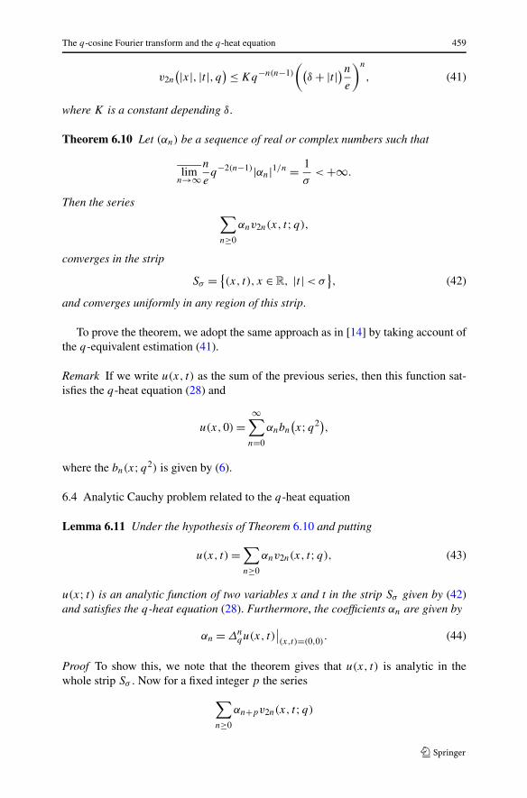
The q-cosine Fourier transform and the q-heat equation 459
v2n
(|x|, |t |, q) ≤ Kq−n(n−1)
((δ + |t |)n
e
)n
, (41)
where K is a constant depending δ.
Theorem 6.10 Let (αn) be a sequence of real or complex numbers such that
limn→∞
n
eq−2(n−1)|αn|1/n = 1
σ< +∞.
Then the series∑
n≥0
αnv2n(x, t;q),
converges in the strip
Sσ = {(x, t), x ∈ R, |t | < σ
}, (42)
and converges uniformly in any region of this strip.
To prove the theorem, we adopt the same approach as in [14] by taking account ofthe q-equivalent estimation (41).
Remark If we write u(x, t) as the sum of the previous series, then this function sat-isfies the q-heat equation (28) and
u(x,0) =∞∑
n=0
αnbn
(x;q2),
where the bn(x;q2) is given by (6).
6.4 Analytic Cauchy problem related to the q-heat equation
Lemma 6.11 Under the hypothesis of Theorem 6.10 and putting
u(x, t) =∑
n≥0
αnv2n(x, t;q), (43)
u(x; t) is an analytic function of two variables x and t in the strip Sσ given by (42)and satisfies the q-heat equation (28). Furthermore, the coefficients αn are given by
αn = Δnqu(x, t)
∣∣(x,t)=(0,0)
. (44)
Proof To show this, we note that the theorem gives that u(x, t) is analytic in thewhole strip Sσ . Now for a fixed integer p the series
∑
n≥0
αn+pv2n(x, t;q)
460 A. Fitouhi, F. Bouzeffour
converges uniformly in any compact region of Sσ . To prove (44), it suffices to seethat for integers n and p we have
(Δn
q,xv2p(x, t;q))∣∣
(0,0)= δn,p,
where δn,p is the Kronecker symbol. �
Finally the following statement is established.
Theorem 6.12 Under the hypothesis of Lemma 6.11, the function u(x, t) given by(43) has the q-Maclaurin expansion
u(x, t) =∑
m,p≥0
βm,p
(1 − q2)m
(q2;q2)mx2ptm,
where
βm,p = αm+pbp
(1, q2). (45)
If for x ∈ R and |t | < σ then function
u(x, t) =∑
m,p
βm,p
(1 − q2)m
(q2;q2)mx2ptm,
satisfies the q-heat equation (28) with the coefficients βm,p given by (44), then u(x, t)
can be extended to an analytic function in the strip Sσ and we have
u(x, t) =∑
n≥0
αnv2n(x, t;q).
Open Access This article is distributed under the terms of the Creative Commons Attribution Licensewhich permits any use, distribution, and reproduction in any medium, provided the original author(s) andthe source are credited.
References
1. Andrews, G.E.: q-Series: Their Development and Application in Analysis, Number Theory, Combi-natorics, Physics, and Computer Algebra. Regional Conference Series in Math., vol. 66. Amer. Math.Soc., Providence (1986)
2. Askey, R., Ismail, M.E.H.: A Generalization of Ultraspherical Polynomials. In: Erdos, P. (ed.) Studiesin Pure Mathematics. Birkhäuser, Basel (1983)
3. Baley, W.N.: Generalized Hypergeometric Series. Cambridge University Press, Cambridge (1935).Reprinted by Hafner Publishing Company (1972)
4. Feinsilver, Ph.: Elements of q-harmonic analysis. J. Math. Anal. Appl. 141, 509–526 (1989)5. Fitouhi, A.: Heat “polynomials” for a singular differential operator on (0,∞). Constr. Approx. 5,
241–270 (1989)6. Gasper, G., Rahman, M.: Basic Hypergeometric Series. Encyclopedia of Mathematics and Its Appli-
cations, vol. 35. Cambridge University Press, Cambridge (1990)7. Haimo, D.T.: Expansion of generalized heat polynomials and their appell transform. J. Math. Mech.
15, 735–758 (1966)
The q-cosine Fourier transform and the q-heat equation 461
8. Ismail, M.E.H.: A simple proof of Ramanujan’s 1ψ1 sum. Proc. Am. Math. Soc. 63, 185–186 (1977)9. Jackson, F.H.: On q-Functions and a Certain Difference Operator. Transactions of the Royal Society
of London, vol. 46, pp. 253–281 (1908)10. Jackson, F.H.: On a q-definite integrals. Q. J. Pure Appl. Math. 41, 193–203 (1910)11. Koornwinder, T.H.: q-Special functions, a tutorial, Mathematical preprint series, Report 94-08,
Univer. Amsterdam, The Netherlands12. Koornwinder, T.H., Swarttouw, R.F.: On q-analogues of the Hankel and Fourier transform. Trans.
Am. Math. Soc. 333, 445–461 (1992)13. Moak, D.S.: The q-analogue of the Laguerre polynomials. J. Math. Anal. Appl. 81, 21–47 (1981)14. Rosenbloom, P.C., Widder, D.V.: Expansions in terms of heat polynomials and associated functions.
Trans. Amer. Math. Soc. 92, 220–266 (1959)15. Swarttouw, R.F.: The Hahn–Exton q-Bessel function, Thesis16. Titchmarsh, E.C.: Introduction to The Theory of Fourier Integrals, 2nd edn. Oxford University Press,
Oxford (1937)


![CHAPTER 11 푸리에광학...11-4 11.2푸리에변환 11.2.1 1차원변환 공간변수를가진1차원함수f(x) [7.56] 푸리에코사인변환및사인변환(Fourier cosine and](https://img.pdfslide.us/doc/110x75/5e5b1f46f4a63f5d502ae408/chapter-11-ee-11-4-112ee-1121-1e-eeeee1fx.jpg)


![B.E Computer Science and Engineering VISVESVARAYA ......Practical harmonic analysis. [7 hours] Unit-II: FOURIER TRANSFORMS Infinite Fourier transform, Fourier Sine and Cosine transforms,](https://img.pdfslide.us/doc/110x75/607e2b5e83f76e5cda62e6bd/be-computer-science-and-engineering-visvesvaraya-practical-harmonic-analysis.jpg)