THE PURCHASING POWER PARITY: EVIDENCE FROM THE

FACULTAD DE CIENCIAS ECONÓMICAS

Y EMPRESARIALES

GRADO EN ECONOMÍA

THE PURCHASING POWER PARITY: EVIDENCE FROM THE GREAT FINANCIAL CRISIS

Autor: Laurentiu Guinea Voinea Tutor : Prof. dr. Juan-Ángel Jiménez-Martín

Curso Académico 2012/2013

24/05/2013

1

“Unless very sophisticated, indeed, PPP is a misleading, pretentious doctrine, promising what is rare in economics, detailed numerical prediction” – P. A. Samuelson “Practical men, who believe themselves to be quite exempt from any intellectual influences, are usually the slaves of some defunct economist.”- John Maynard Keynes

The Purchasing Power Parity: evidence from the Great Financial Crisis

Author: Laurentiu Guinea Voinea Advisor: Prof. dr. Juan-Ángel Jiménez-Martín

2

ABSTRACT The theory of purchasing power parity (PPP) is the simple proposition that states national price levels should tend to be equal when expressed in a common currency, meaning that the nominal exchange rate between two currencies should be equal to the ratio of aggregate price levels between the two countries. The concept of the PPP is based on the law of one price, which says in the absence of transaction costs and official trade barriers, identical goods will have the same price in different markets when the prices are expressed in the same currency. In this paper I analyse the validity of the purchasing power parity (PPP) for four key currencies before and after the Great Financial Crisis against the US dollar. The Euro zone, UK, Canada, and Japan are taken as the domestic country and the US is taken as the foreign country. It has been used two different test methods to check if the Purchasing Power Parity holds. The first method concerns the use of the unit root tests to check the stationarity and non-stationarity of the real exchange rate. If the real exchange rate is stationary, it means PPP holds otherwise does not hold. For this purpose I have used the Augmented Dickey-Fuller unit root test, which has found evidence in favour of purchasing power parity during the crisis period for the UK pound (at 1% confidence interval), for the Euro and the Japanese yen (both at 5% confidence interval). The other method was the two – steps cointegration Engle-Granger test based on the residual test. The results provided the evidence of Purchasing Power Parity holding in the long run only for the Euro (at 5% confidence interval) during the crisis period.

3

Abstract.………..................…...……………………………..…….……………………2

Summary………............................……………………………...………………………3

1. Introduction…………...............……………………………………………...……...3

2. Theoretical backgrounds of the PPP theory…….................…………………...……5

2.1. The Law of One Price……………….............……………………......………...6

3. The PPP in the academic literature……………............................…....………..……9

3.1. The PPP theory – the two variants.………......................…....……......………10

3.2. Deviations from the theoretical model of absolute PPP……...…......................13

4. Theoretical and methodological econometric issues………….................................14

4.1. Unit root: Augmented Dickey-Fuller Test...…………..................……………15

4.2. Cointegration: Engle-Granger test:……………….....................……..….....…17

5. Data description.........................................................................................................19

5.1. Seasonality - Seasonal adjustment ....................................................................20

6. Testing and results ....................................................................................................20

7. Conclusions ..............................................................................................................22

8. References ................................................................................................................23

9. Appendix ..................................................................................................................25

9.1. Box 1: The Balassa- Samuelson effect...............................................................25

9.2. Box 2: The Choice of the Price Index ...............................................................25

9.3. Box 3: Stationarity ............................................................................................26

9.4. Graphical results.................................................................................................27

9.5. Tables.................................................................................................................29

4

1. Introduction

The purpose of this paper is to examine the empirical validity of the purchasing power parity (PPP) theory in the context of the actual Great Recession. Since the early 1970s in the literature there has been an influx of empirical studies on PPP with mixed findings. The main concern of these studies is to find any possible common stochastic trend(s) between exchange rates and relative prices in a bilateral context by employing a number of different unit root and cointegration tests. Purchasing power parity (PPP) is the theory saying that the nominal exchange rate between two currencies should be equal to the ratio of aggregate price levels between the two countries; that is equivalent saying that a unit of currency of one country will have the same purchasing power in a foreign country. Since the 2008 financial crisis, most industrial economies have avoided anything like the collapse that occurred during the Great Depression of the 1930’s due to large-scale fiscal and monetary stimulus. But despite those measures, the advanced economies are still not experiencing any dramatic economic rebound. The actual Brazil’s finance minister, Guido Mantega said that we live a currency dispute that he called the “currency war”. Countries in this war use unconventional ultra-loose monetary policies and money supply expansion with a domino effect of competitive currency devaluations. Yet, because an exchange rate is a relative price, and the PPP is based on the quantity theory, the prices should move in step with the money supply, ceteris paribus. However, given the instability of the money supply - demand since the 2008, the ceteris paribus condition is difficult to be fulfilled. The principal motivation for this investigation is centred on the effects that could have those monetary policies on the exchange rate and on the PPP theory, and analyse if the theory is holding in a period of such high volatility. In this study have been used five of the currencies frequently chosen for testing the PPP hypothesis, and focused the empirical analysis over a time period starting January 1980 and finishing March 2013. The analysis is concentrated over three time windows. The complete sample, which I refer to as the “full sample”, the “pre-crisis sample” which starts January 1980 and ends August 2008, while the third one, the “crisis sample”, is starting September 2008 and runs until March 2013. The currencies chosen are the key currencies of the recent floating exchange rate period: the Euro, the Canadian dollar, the British pound, the Japanese yen, and the US dollar. First step was to check for the stationarity of the real exchange rate before and after the Lehman Brother´s crash in September 2008. For that I used the Augmented Dickey-Fuller unit test and the empirical findings demonstrated that the real exchange rate is not stationary for all currencies with the exception of the UK pound for the crisis period. In base of those results I rejected the hypothesis that the PPP is holding with the exception of the UK pound in the crisis period.

5

To check the evidence for PPP holding in the long run, I employed the Engle-Granger cointegration test that is looking for the equilibrium relationship between variables. The two-steps cointegration test invalidated the PPP hypothesis for all currencies analysed meaning the absence of evidence PPP holding in the long run. This paper is organized as follows: Section 2 reviews the PPP theory´s and the law of one price theoretical backgrounds under its different forms. Section 3 is looking into the academic literature of the PPP hypothesis. Section 4 is presenting the econometric methodology. Section 5 describes the data and presents some empirical evidence based on two different methods. Section 6 summarises the main findings and offers some concluding remarks. 2. Theoretical backgrounds of the PPP theory The PPP theory has a long history in economics, dating back several centuries, starting with the “Salamanca School” and the Spanish doctors of the 16th century who had important contributions to the economic theory. They formulated a quantitative money theory of foreign exchange based on the diversity in the purchasing power in different countries from observing the effects on money supplies, price levels, and exchange rates of large inflows of gold from newly discovered continent, America. The celebrated Augustinian doctor, Martín de Azpilcueta, called “Doctor Navarrus”, made an interesting contribution in introducing the theory of purchasing power of money by observing the phenomena of money and prices in a new vision of a microeconomic framework. In his pioneering work, he equated the “value” of money to its purchasing power, and clarified the point like nobody before him that the “value” or “estimation” of money is determined, in certain circumstances, by its purchasing power1. In its modern form, it was the Swedish economist Gustav Cassel who introduced the specific terminology of “Purchasing Power Parity” in the early twentieth century. During and after the World War I he observed that countries like Germany, Hungary and Soviet Union not only experienced hyperinflation, but also the purchasing power of theirs currencies declined sharply, and the currencies depreciated sharply against more stable currencies like the US dollar. In base on his observations, he proposed a model of Purchasing Power Parity (PPP). That theory became the benchmark for long run nominal exchange rate determination in the years after World War I, especially during the intense debate concerning the appropriate level for nominal exchange rates for countries returning to the Gold Standard but also among the major industrialized

1 Marjorie Grice-Hutchinson, Economic Thought in Spain (1993) – Edward Elgar Publishing Limited, UK

6

countries after phenomena of hyperinflation experienced during and after the World War I (Cassel, 1918). The concept of the PPP is based on the law of one price, which says in the absence of transaction costs and official trade barriers, identical goods will have the same price in different markets when the prices are expressed in the same currency.

2.1. The Law of One Price The idea that PPP may hold because of international goods arbitrage is related to the so-called Law of One Price, which states that the price of an internationally traded good should be the same anywhere in the world once that price is expressed in a common currency, since people could make a riskless profit by shipping the goods from locations where the price is low to locations where the price is high, making a gain by arbitraging. If the same goods enter each country’s market basket used to construct the aggregate price level with the same weight, then the law of one price implies that a PPP exchange rate should hold between the countries concerned. In the long run, there is no evidence why, when converted into the same currency at market exchange rates, the level prices should differ across economically integrated countries. Indeed, when a good is tradable, its price should equalize across countries by virtue of the law of one price. If some price differentials do survive, this must be due to transportation cost, tariffs, or markets imperfections such as imperfect information or monopolistic power. However, if price differentials are structural, they are expected to remain stable or to evolve slowly. Even when they do not, the real exchange rate should revert to a stable level at the aggregate level, based on a macroeconomic adjustment already identified by David Hume in the eighteenth century as the price-specie flow mechanism, a self-stabilizing property of the balance of payments. According to Hume, a country that is enjoying an increase in price competitiveness, normally experience an improvement in its current account. The law of one price, the underlying mechanism behind PPP, is weakened by transport costs and governmental trade restrictions, which make it expensive to move goods between markets located in different countries. Transport costs disconnect the link between exchange rates and the prices of goods implied by the law of one price. As transport costs increase, the larger the range of exchange rate fluctuations. The same is true for official trade restrictions because the customs fees affect importers' profits in

7

the same way as shipping fees. According to Krugman and Obstfeld2, "Either type of trade impediment weakens the basis of PPP by allowing the purchasing power of a given currency to differ more widely from country to country." Let me define formally the law of one price between two countries as follow: by taking for the domestic currency the Euro zone currency, and the United States currency, the dollar, as the foreign currency, we have: PEUi , the price of good i when sold in the Euro

zone, and PUSi the corresponding price in dollars in the US; then the law of one price implies that the euro price of the good i is the same wherever is sold;

PEUi = E€/$ × PUSi (1)

Equivalently, the euro/dollar exchange rate is the ratio of good 𝑖 ´s European and US money prices:

E€/$ = PEUi /PUSi (2)

For the PPP theory, let PEU be the euro price of a reference commodity basket sold in the Euro zone, and PUS the dollar price of the same basket in the US. The PPP predicts a 𝑒𝑢𝑟𝑜/𝑈𝑆 𝑑𝑜𝑙𝑙𝑎𝑟 exchange rate of:

E€/$ = PEU × PUS (3)

We can rearrange the equation in order to get an alternative interpretation of PPP:

PEU = E€/$ × PUS (4)

In the left side of the equation we can see the euro price of the commodity basket in the Euro zone, while the right side we have the euro price multiplied by the euro price of a dollar and that is the euro price of the basket when purchased in the US. Equivalently, the right side measures the purchasing power of a euro when exchanged for dollars and spend in the US. From that expression (3) we can derive that the purchasing power parity explains the movements in the exchange rate between two countries’ currencies by changes in the countries´ price level, while the exchange rate between two countries equals the ratio of the countries’ price levels. PPP therefore holds when, at going exchange rates, every currency´s domestic purchasing power is always the same as its foreign purchasing power.

2 Krugman and Obstfeld (2009). International Economics.Theory and Policy - 8th Edition; Pearson Education

8

Looking at the equation (3) it can be observed that looks like the law of one price, E€/$ = PEU

i / PUSi (2), with the only difference that the law of one price applies to

individual commodities, while the PPP applies to the general price level, which is a composite of the prices of all the commodities that enter into the reference basket. If the law of one price holds for every commodity, of course, PPP must hold as long as the reference basket that in taken into account in the overall price level in every country is the same. While there has been much controversy about the general validity of PPP, the theory does in fact highlight important factors behind the exchange rate movements. One very simple way of gauging whether there may be discrepancies from PPP is to compare the prices of similar or identical goods from the basket in the two countries. Since 1986, the “Economist” publishes the prices of McDonald’s Big Mac hamburgers around the world and compares them in a common currency, the U.S. dollar, at the market exchange rate as a simple measure of whether a currency is overvalued or undervalued relative to the dollar at the current exchange rate. The supposition was that the currency would be valued just right if the dollar price of the burger were the same as in the U.S. The Big Mac index was invented in the light of applying the economic theory to real goods. It was never intended as a precise measure of currency misalignment, but only as a tool to make exchange-rate theory more easily digestible. Yet the Big Mac index has become a global standard, included in several economic textbooks and the subject of at least 20 academic studies. It is based on the pure theory of purchasing-power parity (PPP), the notion that in the long run exchange rates should move towards the rate that would equalise the prices of an identical basket of goods and services (in this case, a burger) in any two countries. For example, at the start of 2013, the "raw" Big Mac index says that the Chinese yuan was undervalued by 41% against the dollar, the euro was 11.69 per cent overvalued, and the Japanese yen was 19.54 per cent undervalued on the Big Mac PPP standard. The same newspaper “Economist”, however, is testing whether a new index based on coffee instead of burgers reaches the same conclusions. The Starbucks “tall-latte index” tells broadly the same story as the Big Mac index for most main currencies. It should be called “broadly”, because they are distorted by differences in the cost of non-tradable such as rents, wages, and taxes that differ from country to country.

9

3. The PPP in the academic literature There is a vast literature written on the PPP hypothesis. Since the early 1970s, the PPP theory has been the subject of an on going and lively debate. In the 1980s, economists would usually argue that PPP does not hold even in relative terms or even in the long run. This conclusion was based on time series analyses of key exchange rates over the 1970s and 1980s. Since the 1990s, longer time and higher-frequency series, together with the use of panel-data analysis that involve an increase in the number of observations included in the regressions, have led to a different conclusion. It has increasingly been recognized that there is some mean-reversion toward a stable real exchange among the most advanced economies, although the convergence is very slow. On average it takes three to five years to close half of the gap between the real exchange rate and its long-term value, absent new shocks (Rogoff, 1996). The theoretical work suggested that exchange rates should be linked to relative changes in price levels with deviations that might be only minimal or momentary, while empirical work could hardly find evidence in support of purchasing power parity (Abuaf and Jorion 1990). Even so, the idea of PPP has become embedded in the economists thinking. For example, Dornbusch and Krugman (1976) noted: “Under the skin of any international economist lies a deep-seated belief in some variant of the PPP theory of the exchange rate.” Rogoff (1996) expressed much the same thought: “While few empirically literate economists take PPP seriously as a short term proposition, most instinctively believe in some variant of purchasing power parity as an anchor for long-run real exchange rates.” R. Dornbusch stated in 1985 in a famous paper that the Purchasing Power Parity (PPP) is a “theory of exchange rate determination”3 and the change in the relative price levels between two countries would determine changes of the exchange rate. As it´s based on the price levels changes as the main factor of the exchange rate movements, it has been also called the “inflation theory of exchange rate”. However, it is often asserted that the PPP theory of exchange rates will hold at least approximately because of the possibility of international goods arbitrage. From an historical standpoint, there have been numerous studies of PPP for various countries over the period in question, some covering a particular era or monetary regime. Lately, new studies have appeared in abundance. In a comprehensive review of the purchasing-power parity literature, Froot and Rogoff (1995) could declare that what was a “fairly dull research topic” only a decade ago has recently been the focus of substantial controversy and the subject of a growing body of literature. Recent empirical research, mostly based on the time-series analysis of short spans of data for the floating-rate (post-Bretton Woods) era led many to conclude that PPP failed to hold, and that the real exchange rate followed a random walk, with no mean-reversion property. However, a newly emerging literature exploits more data and higher-powered techniques, and

3 R. Dornbusch, Purchasing Power Parity (1985)- National Bureau of Economic Research; Working Paper No. 1591

10

claims that, in the long run, PPP does indeed hold: it appears from these studies that real exchange rates exhibit mean reversion with a half-life of deviations of four to five years (M. P. Taylor 1995; Froot and Rogoff 1995). It can be discerned that is a clear evolution in the methodology to assess the validity of this hypothesis. First the parity was investigated in a univariate framework. However, due to the low power of the unit root test the null hypothesis of a unit root does not need to be rejected even if the real exchange rate is in fact stationary (Lothian and Taylor (1996)). According to Froot and Rogoff (1995) stationary (monthly) data covering a period of 72 years are needed to accept PPP with a half-life of three years. However, most exchange rate data covering such lengthy period are sampled under a fixed and floating exchange rate regime. Under a fixed regime, the exchange rate is fixed by one of the authorities of the underlying countries while under a floating regime the exchange rate is determined by supply and demand. Most of the developed countries follow a floating regime. The classical example of a fixed exchange rate regime was the Bretton Woods fixed exchange rate system that lasted from 1946 to 1973. It is very clear that the behaviour of the exchange rate is different under a fixed or floating regime thereby contaminating inferences made on the PPP hypothesis. The present crisis provided enough evidence to affirm that real shocks can cause temporary deviation from the PPP by monetary disturbances effects transmitted to relative price levels and exchange rates. However, as the monetary policy has no effect in the long run on the real exchange rates, we expect that the bilateral exchange rate to adjust these differentials and that in the long run the PPP would converge. While in the short run the deviations from the PPP are important, there is evidence in the economic literature that the half-life of deviations from PPP is a period between 3 and 5 years for the exchange rate among the most developed economies.

3.1. The two variants of the PPP theory PPP theory has two main variants, two senses in which the PPP hypothesis might hold, the absolute and the relative hypothesis. Absolute purchasing power parity hypothesis could be resumed in the simply formula of the price ratio equals the exchange rate. That hypothesis holds when the nominal foreign exchange rate between two currencies is such that the purchasing power of a unit of currency is exactly the same in the foreign economy as in the domestic economy, once it is converted into foreign currency at that rate (Isard 1995). The absolute PPP hypothesis states that the exchange rate between the currencies of two countries should equal the ratio of the price levels of the two countries.

11

Specifically: S = P /P* (5)

Where S is the nominal exchange rate (spot exchange rate) measured in units of foreign currency per unit of domestic currency, P is the domestic price level, and P* is the foreign price level. Equivalently, absolute PPP implies that the nominal exchange rate between two currencies is equal to the ratio of national price levels. Relative PPP hypothesis holds when the percentage change in the exchange rate over a given period just offsets the difference in inflation rates in the countries concerned over the same period. In this way the purchasing power of a unit of the domestic currency in the domestic economy relative to its purchasing power in the foreign economy when converted at the going exchange rate is the same at the end of the period as at the beginning of the period. Relative PPP states that the change in the exchange rate should equal the difference in inflation rates (change in prices). In this case the real exchange rate should be constant over time (not necessarily equal to one). The relative PPP hypothesis states that the exchange rate should bear a constant proportionate relationship to the ratio of national price levels, in particular:

S = kP /P* (6) where k is a constant parameter. Either variant implies a constant real exchange rate (Q):

Q = SP* /P (7) If we take logarithms of both sides of the equations of (5) and (6) we reach:

s = c+ p* − p (8) where s, p*, p are the logarithms of S,P*,P and c = ln(k)= 0 under absolute PPP. Under either variant of PPP, a change in the ratio of price levels implies an proportionate change in the nominal exchange rate, such that:

Δs = Δp* − Δp (9) The above expression (9) says that the percentage change in the nominal exchange rate is equal to the difference between the inflation rates in the domestic and the foreign country. The PPP could also be interpreted as that the difference in the rate of change in prices at home and abroad, seen as the difference in the inflation rates, that should be equal to the percentage depreciation or appreciation of the exchange rate.

12

Absolute purchasing power parity holds when the purchasing power of a unit of currency is exactly equal in the domestic economy and in a foreign economy, once it is converted into foreign currency at the market exchange rate. Even so is evident that the PPP exchange-rate calculation is controversial because of the difficulties of finding comparable baskets of goods to compare purchasing power across countries. Deviations from parity imply differences in purchasing power of a "basket of goods" across countries, which means that for the purposes of many international comparisons, countries' GDPs or other national income statistics need to be "PPP-adjusted" and converted into common units. However, it is often difficult to determine whether literally the same basket of goods is available in two different countries. Thus, it is common to test relative PPP, which holds that the percentage change in the exchange rate over a given period just offsets the difference in inflation rates in the countries concerned over the same period. If absolute PPP holds, then relative PPP must also hold; however, if relative PPP holds, then absolute PPP does not necessarily hold, since it is possible that common changes in nominal exchange rates are happening at different levels of purchasing power for the two currencies (perhaps because of transactions costs, for example). In theory, any deviation from PPP should result in an immediate change in prices and/or the exchange rate in such a way that the parity still holds. However, due to barriers like transaction costs, non-tradability etc., PPP does not hold perfectly in practice. The theoretical consensus is that these deviations are supposed to be temporary so that prices should converge to each other. This means that the real exchange rate should be mean-reverting/stationary and should not contain a unit root; after the real exchange rate is affected by an exogenous shock (whether caused by a change in prices or a change in the nominal exchange rate), the series should return to its mean level. The degree to which mean reversion takes place is often measured by the half-life which denotes the time needed for the series to return to a level that equals half the size of the original shock. Even if the law of one price holds, PPP need not do so. We can observe that trough a purely statistical phenomenon: if the weights given to various goods in the calculation of the price index differ among the countries, and divergent price developments of goods result in divergent price index movements, the law of one price could hold for all goods and the bundles of goods on which the price is calculated are identical.

13

3.2. Deviations from the theoretical model of absolute PPP Purchasing power parity is both a theory of exchange rate determination and a tool to make more accurate comparisons of data between countries. It is probably more important in its latter role since as a theory it performs pretty poorly. Its poor performance arises largely because its simple form depends on several assumptions that are not likely to hold in the real world:

• It´s based on a simplistic model that doesn’t take into account the transportation costs and tariffs, the differences in the consumption patterns between countries, non-traded goods and services.

• It´s based on the Efficient Market Hypothesis. The reality shows as everyday that we are living in an Imperfect markets world economy, and especially the sticky prices wont allow markets to work efficiently.

• There are also statistical difficulties, like the construction of price indexes,

where the goods in the baskets in different countries are not homogenous, and also price index includes tradable and non-tradable goods.

Since the Great Recession, we have noticed consumption patterns change within countries and that changed the relative price of tradable to non-tradable goods. The causes of such a change in the relative prices reflected in the money – demand can be thought of:

• The Balassa-Samuelson effect [Insert Box 1]

• Shifts in the consumer preferences

• Different percentages of government spending in GDP, highly oriented in social

transfers that are mainly non-tradable like social services, health, pensions and education.

• International capital flows, mainly from developed countries to BRICS countries due to the differentials in the interest rate.

• Real monetary shocks - unconventional monetary policies and money supply expansion (quantitative easing).

14

4. Theoretical and methodological econometric issues

In order to look for the Great Recession´s effects, I applied empirical analysis over three sample periods. The first sample, which I refer to as the “full sample”, runs from January 1980 until March 2013, the “pre-crisis sample”, starts January 1980 and ends in August 2008, while the third one, the “crisis sample”, is starting September 2008 and runs until March 2013. In this paper, I am going to test: 1) the relative hypothesis PPP by checking the stationarity of the real exchange rate and 2) and the long run PPP by testing if is there a stable relationship among the exchange rate and the level of prices. My approach starts from a simple model, which takes the form of the equation (8). Based on that, the following linear versions of the PPP relationship has been considered:

st = β0 + β1pt + β2pt* + et (10) where st is the natural logarithm of the nominal exchange rate expressed in terms of the

domestic price of foreign exchange, pt and pt* are the natural logarithm of the domestic and US CPI, respectively. From the expression (10) we can derive the following conclusions:

i) The absolute PPP hypothesis requires that et in (10) be a stationary process,

meaning that, st , pt , pt* should be cointegrated (Engle and Granger, 1987).

ii) If in the expression (10) we impose the restriction of β1 = −β2 = β , then we could prove the relative PPP hypothesis that would require the stationarity of the real exchange rate. For that would be needed that β0 = 0,β =1 and the expression could become (where et would be the real exchange rate):

st − (pt − pt*)= et (11) As mentioned in the equation (10) and in the point ii), my model requires that the real exchange rates be stationary. If real exchange rates are found to have a unit root, this implies a violation of PPP. Otherwise the real exchange rate will be stationary or mean reverting and the PPP theory in the relative form holds (Jiménez-Martin and Robles-Fernández 2009). The real exchange rate is defined as the nominal exchange rate deflated by a ratio of domestic to foreign price levels as follow:

Real Exchange Ratei/$ = Nominal Exchange Ratei/$ ×Consumer Price Indexi

Consumer Price IndexUS (12)

15

Corresponding to the concept in equation (12), I first construct the real exchange rates, for the Euro zone, Canada, Japan and United Kingdom, using the United States as the base country.

[Insert Box 2] By taking logarithms on the real exchange relationship (12) we have:

ln(e)= ln(SP /P*)⇒ e = s + p− p* (13) where e is the log of the real exchange rate, s is the log of the spot exchange rate defined in local currency units per foreign currency unit, and p and p* are the log of the CPI, with asterisks denoting the logarithm of the US CPI. Let consider that the real exchange rate is specified as a first-order autoregressive process, where the variable is regressed level. If the coefficient on the lagged level is below one, the real exchange rate is stationary and PPP holds. If the coefficient equals one, the real exchange rate has a unit root and PPP does not hold. Following this model´s reasoning, therefore, I use the Augmented Dickey-Fuller (ADF) unit root test to check the variables stationarity and verify that each of these series is integrated of order one. To fully understand the implications for empirical modelling of having unit roots in the data, in the appendix are mentioned the statistical properties of stationary and non-stationary processes.

[Insert Box 3]

4.1. Unit Root: Augmented Dickey-Fuller Test; The unit roots are omnipresent in economics and business time series data4; most of the macroeconomic aggregates such as GDP, consumption, interest rates, stock prices and so have at least one unit root. This is somehow expected because all those variables, although measuring different aspects of the economy, are closely related. In my case, both the exchange rate and consumer price indexes must be checked for the unit root. The unit root test is the formal test for checking the non-stationarity in the time series data. There are several type of Unit Root Test like the Augmented Dickey-Fuller (ADF) test, the Phillips-Perron (PP) test, the Dickey-Fuller Generalised Least Squares (DF-GLS) test, or the KPSS Test.

4 I many cases the economic time series are non-stationary, and at best become stationary only after differencing. A stationary process can be autocorrelated but such that the influence of past shocks dies out, although the variance would not be constant.

16

The simple Dickey-Fuller test for unit roots Dickey and Fuller (1979, 1981) devised a procedure to formally test for non- stationarity based on the simple AR(1) model of the form:

Yt = φYt−1 + ut (14) What we need to examine here is whether ϕ is equal to 1 (unity and hence 'unit root'). The null hypothesis is H0 :φ = 1 , and the alternative hypothesis is H1 :φ <1 By subtracting Yt−1 from both sides of:

Yt −Yt−1 = φYt−1 −Yt−1 + ut

ΔYt = (φ −1)Yt−1 + ut which can alternatively can be written as:

ΔYt = βYt−1 + ut (15)

where β = (φ −1)and Δ is the first difference operator. Then, now the null hypothesis is H0 :β = 0 and the alternative hypothesis is H1 :β < 0 . If β = 0 , then φ = 1 , that is there we have a unit root, meaning the time series under consideration is non-stationary. Dickey and Fuller (1979) also proposed an alternative regression equation that can be used for testing for the presence of a unit root. This equation contains a constant in the random-walk process as in the following equation:

ΔYt =α 0 + βYt−1 + ut (16) In this paper I will use the Augment Dickey Fuller (ADF) test. This test is conducted by “augmenting” the equation (16) by adding the lagged values of the dependent variable ΔYt :

ΔYt =α 0 + βYt−1 + γ ii=1

m∑ ΔYt−1 + ut (17)

where ut is a pure white noise error term and where:

ΔYt−1 = (Yt−1 −Yt−2 ),ΔYt−2 = (Yt−2 −Yt−3),etc.

The number of lagged difference terms to include is often determined empirically following the idea to include enough terms so that the error term is serially uncorrelated. EViews8 has an option that automatically selects the lag length based on Akaike,

17

Schwarz and other information criteria. If the coefficient of a lagged variable shows a value of one, then the equation show the sign of non-stationary. The null hypothesis is written as:

𝐻!:𝜙 = 1 (𝑛𝑜𝑛 − 𝑠𝑡𝑎𝑡𝑖𝑜𝑛𝑎𝑟𝑖𝑡𝑦) 𝐻!:𝜙 < 1 (𝑠𝑡𝑎𝑡𝑖𝑜𝑛𝑎𝑟𝑖𝑡𝑦)

Under the null hypothesis of unit root, the z-ratio is not normal distributed and has a nonstandard density function known as the Dickey–Fuller distribution. The shape of this distribution is completely different from the normal distribution, as is asymmetric and skewed to the left, with a long tail, making it hard to discriminate the null of a unit root from alternatives close to unity. The decision rule:

• If t-statistic > ADF critical value, means: fail to reject the null hypothesis, unit root exists.

• If t-statistic < ADF critical value, means: reject the null hypothesis, unit root does not exists.

If we fail to reject the null Hypothesis, we assume that there is a unit root and difference the data before running a regression. If the null is rejected, the data are stationary and can be used without differencing. The empirical validity of the PPP will be tested over the all three time windows, for a model that has the following form:

Yt = c+Yt−1 + εt (18)

As an alternative, it could be written also as:

ΔYt = Yt −Yt−1 = c + ε t (19)

If the null hypothesis of the first unit root is rejected, then I will check for the ADF unit root test in first difference that is expected to be stationary. In the case there would be additional unit roots, the first difference of the series ΔYt would be also non-stationary. Before setting the final model, we need to check for additional unit roots running the ADF test on additional differences. The model in differences has the following form:

ΔYt = c+βYt−1+εt (20)

When trying to answer the question whether long-run purchasing power parity holds, a number of tests are available to examine the relationship between the nominal exchange

18

rate and the price level5. As in most previous empirical studies, I will examine the linkages between the variables by using the OLS regression analysis. However, some studies employed the Engle-Granger two-step cointegration6 approach or the Johansen full-information maximum likelihood technique to explore the long-run relationship.

4.2. Cointegration; Engle-Granger test The cointegration techniques have been a dominant force in applied macroeconomics. The key motivation for using the cointegration analysis is to avoid spurious regression results. In addition, those techniques play a useful role in identifying meaningful long-run economic relationships among non-stationary variables. In 1987, Engle and Granger showed that it is possible for a linear combination of integrated variables to be stationary and thus integrated at a given lower order7. In order to demonstrate that, they developed a simple test that is done by first running the “co-integrating regression” using OLS, and then test if the residual in the estimated equation comes out being is stationary. If it is stationary, it indicates that there is a stationary cointegrating relationship. In this paper I will employ the Engle-Granger cointegration test that generally takes two steps. The first step is to conduct a unit root test8 in order to determine the time series behaviour of the variables; that test will also confirm the order of integration for a given variable. If all variables are integrated of the same order, the second step is to estimate

5 If you are estimating a model that includes time series variables, the first thing you need to make sure is that either all time series variables are stationary or they are cointegrated. In the case they are integrated of the same order and errors are stationary, the model defines a long run equilibrium relationship among the cointegrated variables. 6 Murray (1994) introduced a humorous example that helps to visualise the cointegration. He described a drunk and her dog for demonstrating the behaviour of a cointegration in bivariate time series. By using the traditional example of the meandering or 'random walk' of a drunken man he provided a demonstration of a simple non-stationary process as they both follow non-stationary paths. If two time series variables are non-stationary, but cointegrated, at any point in time the two variables may drift apart, but there will always be a tendency for them to retain a reasonable proximity to each other. 7 It is necessary for the cointegration test that the order of integration of all the variables in the long run will be the same. The order of integration is the number of times, a time series variables must be difference for it to become stationary. Non-stationary series that become stationary when differenced n times are called integrated of order n. For a set of series to be cointegrated, each member of the set must be integrated of the same order, n. A set of series, all integrated of order n, are said to be cointegrated if and only if some linear combination of the series is integrated of order less than n. 8 The unit-root assumption implies an ever-increasing variance to the time series, around a fixed mean, violating the constant-variance assumption of a stationary process. The errors persist indefinitely, and past errors accumulate with no `depreciation', containing all information of the past behaviour up to first observation. The variance of a unit-root process increases over time, and successive observations are highly interdependent.

19

the model, also called a “cointegrating equation,” and test whether the residual of the model is stationary. Applied to my model and according to the cointegration method, the PPP hold in the long run if the sum between the nominal exchange rate and US´s CPI are cointegrated with the CPI of the domestic country, meaning that I will be looking for a linear combination of the two series that is stationary. Having tested the unit root, the next step is estimating an OLS model on the I(n) variables, and the PPP relation for the Engle-Granger is:

log(ei ) = log(pi )+ log(pUS ) (21) In linear econometric model form, after adding stochastic deviations:

log(eit ) = β0 + β1 log(pi )+ β2 log(pUS )+ ε t (22)

where the i sub index stays for the different countries: the Euro zone, Canada, Japan, and UK. The residuals of the equation (22) have to be saved, and tested whether the first order autocorrelation coefficient has a unit root - they are cointegrated or not. Like the unit root tests, the cointegration tests also have non-standard distributions, and all the issues concerning unit root testing apply here as well. 5. Data description The primary source of data is the International Monetary Fund’s International Financial Statistics (IFS), downloaded from the Economic version of the Reuters EcoWin Pro. My data set includes monthly averages of the exchange rates (nominal) in local currency per US dollar, as well as consumer price indices (CPI) proxying for price levels. The Canada, Japan, United Kingdom (UK) and the United States (US) data sample contains observations from January 1980 to March 2013, while the Euro zone data set is running from the inception of the euro, January 1999 to March 2013. The set amounts 399 data points. The CPI series are presented in indexes, and the exchange rates series are exchange rates for the euro/dollar, the Canadian dollar/ US dollar, British pound/US dollar, and Japanese yen/US dollar. The Table 1 (Appendix) shows the descriptive statistics of the real exchange rate in the first difference. It is interesting to mention that the mean for the Euro and UK pound is higher in the “crisis period” than the “pre-crisis period”, while the Japanese yen shows

20

much lower the standard deviation in the “crisis” period than the “pre-crisis period”. I would remark also that the skewness of the Euro, Japanese yen and UK pound is negative for the pre-crisis period, and becoming positive during the crisis.

[Insert Table 1]

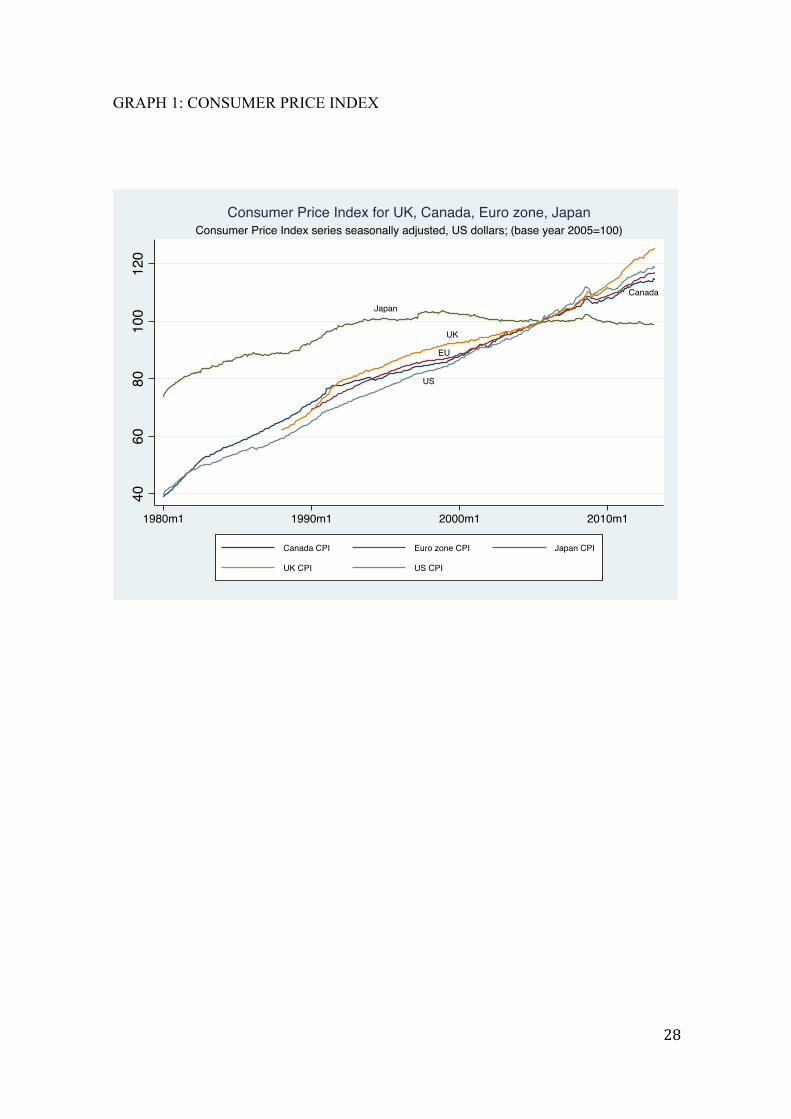
As said by Enders (1995), the visual inspection of the data is a critical first step in any econometric analysis. To get a feel for to the real world, start with Graph 1 (Appendix) that plots data on Euro zone, Canada, Japan, the U.K., and the U.S. consumer price indices (CPIs) over the period 1980–2013, having the base year 2005=100. All are expressed in U.S. dollar terms, which means that the countries CPI was multiplied by the number of U.S. dollars exchanging for one unit at that point in time. Inspection of the graph of the price indexes indicates that the series have an increasing trend for all the five countries with a very high correlation between all national price levels with the exception of Japan.

[Insert Graph 1]

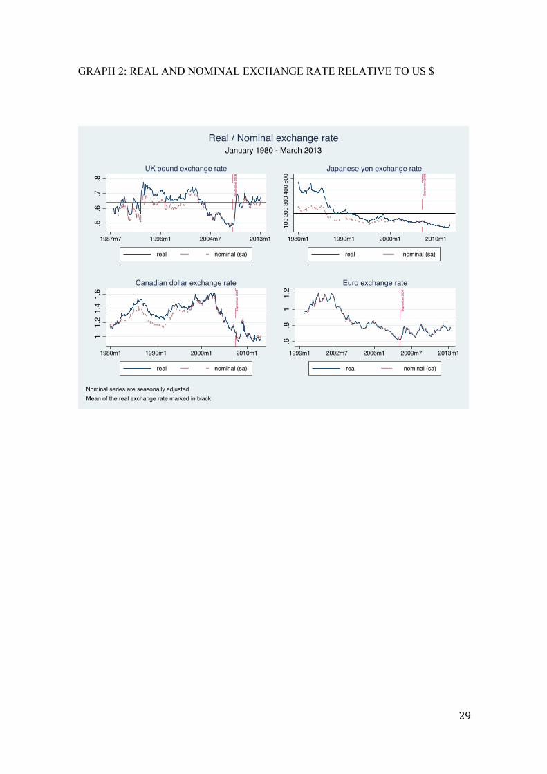
Graph 2, shows the real and nominal exchange rates for the four currencies analysed against the US dollar. It can be noticed that each exchange rate has showed large and persistent deviations around its mean. Nevertheless, during the crisis period the exchange rates considered seem to stabilize around a lower mean, and having a lower standard deviation.

[Insert Graph 2]

5.1. Seasonality – Seasonal adjustment It is a very well known fact that many economic and financial time series display seasonality; seasonality can be defined as a pattern of a time series, which repeats at regular intervals every year9. If ignored and not treated, the seasonality could obscure movements of the exchange rates statistically important, and since the beginning was desirable to remove this interference component, otherwise is possible to obtain a spurious relationship between the Consumer Price Index series and the exchange rate series. As the nominal exchange rates, and CPI data series, downloaded from EcoWin Pro Economic database where not seasonally adjusted, the choice of method for seasonal adjustment is crucial for the removal of all seasonal effects in the data. I applied the seasonal adjustment filter, the X-13ARIMA-SEATS that is included in

9 Seasonal fluctuations in data make it difficult to analyse whether changes in data for a given period reflect important increases or decreases in the level of the data, or are due to regularly occurring variation. In search for the economic measures that are independent of seasonal variations, methods had been developed to remove the effect of seasonal changes from the original data to produce seasonally adjusted data. The seasonally adjusted data, providing more readily interpretable measures of changes occurring in a given period, reflects real economic movements without the misleading seasonal changes.

21

Eviews8 software 10 . The X-13ARIMA-SEATS is seasonal adjustment software produced, distributed, and maintained by the Census Bureau, US. This method, originally developed by Victor Gómez and Agustín Maravall at the Bank of Spain, has the capability to generate ARIMA model-based seasonal adjustment using a version of the SEATS procedure. 6. Testing and results At this point, having defined the methodology, I run the test to check the stationarity and non-stationarity of the real exchange rate. Using the EVIEWS 8 software, is performed the ADF test for the “full sample period”, “pre-crisis period” and “crisis period”. The model is in levels, with intercept and trend, and the ADF statistic is compared with 1% and 5%, critical value, in order to determine if it falls within the acceptance region.

[Insert Table 2]

Table 2 shows the results of applying the augmented Dickey-Fuller (ADF) unit root tests to the real exchange rate series on levels and first difference. The results found that during the “crisis period” the UK pound is stationary at 1% confidence interval, while the Euro and the Japanese yen are stationary at 5% confidence interval. The Table 2 present also the results for the unit root in the first difference. For the all other cases, the unit root was rejected, and the series are said to be stationary and integrated of order one, I (1)11. The summary of the results from the Table 2:

• The full sample: The data reveals that the augmented Dickey-Fuller statistic lays inside the acceptance region at 1% and 5% for all series tested. Therefore, I fail to reject the presence of unit root for all the four series tested and real exchange rates have been found to be non-stationary based on an efficient unit root test on levels. The PPP is not holding for the “full sample” period.

• The pre- crisis period: The data reveals that the augmented Dickey-Fuller statistic lays inside the acceptance region at 1% and 5% for all series tested. Therefore, I fail to reject the presence of unit root for all the four series tested and real exchange rates have been found to be non- 10 The additive decomposition used for seasonal adjustment is 𝑦! = 𝑆! + 𝑇! + 𝐼!, where 𝑦! is the observed time series, and 𝑆! ,𝑇! , 𝑎𝑛𝑑 𝐼! are the seasonal, trend, and irregular components. 11 If a series needs to be difference n times before it becomes stationary then it contains n unit roots and is said to integrated of order n that is I(n).

22

stationary based on an efficient unit root test on levels. The PPP is not holding for the pre-crisis period.

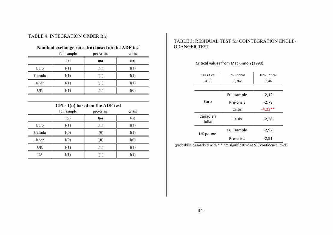
• The crisis period: The data reveals that the augmented Dickey-Fuller statistic lays outside the acceptance region at 1% for the UK pound, while for the Euro and the Japanese yen at 5%. Therefore, I reject the presence of unit root for the UK, Euro and Japanese yen, and real exchange rate has been found to be stationary based on an efficient unit root test on levels. Based on the ADF test, the PPP hypothesis is only holding the for UK pound, Euro and Japanese yen during the crisis period. Prior last step of my analysis, testing for cointegration, the nominal exchange rate and the CPI series are tested to determine their order of integration, in levels as well as in first differences. While the tables 3a and 3b show the results achieved by estimating the ADF unit root tests with a constant, the table 4 shows the integration order I(n) of the variables. Due to differences in the integration order between the nominal exchange rate series and the US CPI, there was possible to test for cointegration for the Euro zone (full sample, pre-crisis, and crisis), UK (full sample and pre-crisis) and Canada (crisis). The Japanese yen was excluded from testing the cointegration because the Japanese CPI is stationary and integrated of I(0) over the three time periods.

[Insert Table 3a, 3b, and 4)] The Table 5 presents a summary of the results for the standard unit-root tests on the residuals (ADF tests) resulted from the equation (22), based on the critical values from MacKinnon(1990):

[Insert Table 5]

• The Euro zone: Reject the null hypothesis for the ADF test of the residual for the crisis period at 5%.

• The UK: failed to reject the null hypothesis the ADF test of the residuals for the full sample and the pre-crisis period.

• The Canada: failed to reject the null hypothesis for the ADF test of the residual for the crisis period.

The residual test´s provided a weak evidence of the PPP hypothesis holding for the Euro, while for all other currencies analysed the conclusion is there is no evidence of cointegration in the long run.

23

7. Conclusion

The purpose of this paper is to determine the validity of the PPP hypothesis for four key currencies of the recent floating exchange rate period. I have been using two different approaches for the empirical study: (a) the unit root test for the stationarity of real exchange rates and (b) the cointegration test between price indexes and nominal exchange rates. The data do reveal difference between the two periods object of my paper. The PPP in the relative form in either series for the “full sample” and “pre-crisis period” that doesn´t hold as I failed to reject a unit root trough the ADF test. For the “crisis period” I reject the non-stationarity of the UK pound, Euro and Japanese yen. These results provide evidence that purchasing power parity holds during the crisis period for the UK pound, Euro and the Japanese yen. The Engle-Granger test failed to reveal that there exists a cointegrating relationship, which links the Canadian dollar, Japanese yen, the UK pound and the US prices. Only for the Euro during the crisis period there is evidence in support of the existence of a long-term relation between nominal exchange rate and CPIs, with a cointegration vector that is compatible with PPP. The results confirm that neither of the two traditional approaches to testing for PPP could solve definitely the issue of the PPP. These findings would not validate the hypothesis that the nominal exchange rate and relative prices share a common trend so that the real exchange rate is a mean reverting stationary process. Hence, deviations that are attributed to transitory monetary shocks, will translate into real exchange rate variability. Since the real exchange rate is a combination of price levels and exchange rates, any shocks arising in the financial market that move the nominal exchange rate are passed on to the real exchange rate due to sticky prices.

24

References: Abuaf, N. and Jorion P. (1990). Purchasing Power Parity in the Long Run. Journal of Finance. 45, p157-74. Balassa, Bela. (1964). The Purchasing-Power-Parity Doctrine: A Reappraisal. Journal of Political Economy. 72, p584-96. Cassel, Gustav (1918), .Abnormal deviations in international exchanges. The Economic Journal. 28, p413-15. Dickey, D. A. and Fuller, W. A. (1979). Distribution of the estimators for autoregressive time series with a unit root. Journal of the American Statistical Association. 74, p427-431. Dickey, D. A. and Fuller, W. A. (1981). Likelihood ratio statistics for autoregressive time series with a unit root. Econometrica. 49, p1057-1072. Froot, K. A. and K. Rogoff (1995). Perspectives on PPP and Long-Run Real Exchange Rates in Grossman, G. and K. Rogoff (eds), Handbook of International Economics, Vol. III, North-Holland, Amsterdam, 1647-88. Lothian, J.R. and Taylor M. P. (1997). Real exchange rate behavior. Journal of International Money and Finance. 16 (6), p945-54. Isard, Peter. (1995). Exchange Rate Economics (Cambridge: Cambridge University Press). Jiménez-Martin, Juan-Angel and Robles-Fernández, M.D.. (2009). PPP: Delusion or Reality? Evidence from a Nonlinear Analysis. Open Economies Review Krugman and Obstfeld (2009). International Economics.Theory and Policy - 8th Edition; Pearson Education Marjorie Grice-Hutchinson, Economic Thought in Spain (1993) – Edward Elgar Publishing Limited, UK. MacKinnon, James G. 1990. Critical Values for Cointegration Tests, Working Papers 1227, Queen's University, Department of Economics. Murray, M.P. (1994). A Drunk and Her Dog: An Illustration of Cointegration and Error Correction. The American Statistician. 48, p37-39.

25

Mussa, Michael. (1984). The Theory of Exchange Rate Determination. Exchange Rate Theory and Practice. ed. by John F.O. Bilson and Richard C. Marston, p13-78. Chicago: University of Chicago Press. Samuelson, Paul A. (1964). Theoretical Notes on Trade Problems. Review of Economics and Statistics. 46, p145-54. Taylor, Alan M. and Taylor, Mark P. (2004). The Purchasing Power Parity Debate. CRIF Seminar series. Paper 24. Taylor, A.M. (2002). A Century of Purchasing Power Parity. The Review of Economics and Statistics. 84, p139-150.

26

APPENDIX Box 1 The Balassa- Samuelson effect An important modification of the PPP approach has come from the effect associated with Balassa (1964) and Samuelson (1964) work. In the same year, 1964, and in separate contributions, they highlighted the role of the productivity differentials in explaining differences in price levels. They observed that the prices of non-tradable goods and services, relative to prices of tradable, tend to be lower in low-income countries than in high-income countries. The Balassa-Samuelson hypothesis, states that the relative price of non-tradable tend to be higher in high-income countries due to a faster rise in the productivity of the tradable goods sector relative to productivity in the non-tradable sector as economies develop and real incomes grow. Given competitive pressures within countries for workers with similar skills to receive similar wages in the two sectors, relatively rapid productivity growth in the tradable sector, other things equal, would tend to push up the relative cost of production in the non-tradable sector and, hence, the relative price of non-tradable Box 2 The Choice of the Price Index: Most studies investigated the validity of PPP for a basket of goods at an aggregate level using consumer and/or producer price indices instead of for individual goods (although there are exceptions of the latter such as the mentioned before, the Big Mac Index, or the Starbucks “tall latte index”, published both by the Economist). The most commonly used price series used in constructing real exchange rates are consumer price indices (CPIs). These have the advantage of being timely, similarly constructed across countries and available for a wide range of countries over a long time span. The consumer price index (CPI) is an index that measures the average level of prices of goods and services in an economy relative to a base year. To track only what happens to prices, the quantities of goods purchased are assumed to remain fixed from year to year. This is accomplished by determining—with survey methods—the average quantities of all goods and services purchased by a typical household during some period. The quantities of all of these goods together are referred to as the average market basket. In practice, different price indices can be used in the calculation of the real exchange rates on the basis of purchasing power parity. The wholesale price index (WPI) and the consumer price index (CPI) are two of the leading indices that can be used in these

27

calculations. The gross domestic product (GDP) deflator and producers price index (PPI) are also among the alternatives. Box 3 Stationarity: A time-series variables that posses a constant mean and a constant variance over time and the autocorrelation function that depends solely on the length of the expressed lags is known as stationary time series. A time series variable that satisfy the following properties is said to be covariance or weakly stationary: 1 𝐸 𝑌! = 𝜇 𝑓𝑜𝑟 𝑡 = 1,2,3,…∞ ; meaning Time Independent Mean [constant for all

t] 2 𝑉𝑎𝑟 𝑌! = 𝜎! ;Time Independent Variance [constant for all t]

3 𝐶𝑜𝑣 (𝑌! − 𝑌!!!) = 𝛾! ;Constant for all t and t-1

So if the Process is covariance Stationary, all the variances are the same and all the covariance depends on the difference between t and t-s. For a stationary time-series, the autocorrelation functions (ACF) tend to zero rather quickly, while for a non-stationary the ACFs are better described by a linear decline.

28

GRAPH 1: CONSUMER PRICE INDEX

Japan

UK

US

Canada

EU

4060

8010

012

0

1980m1 1990m1 2000m1 2010m1

Canada CPI Euro zone CPI Japan CPI

UK CPI US CPI

Consumer Price Index series seasonally adjusted, US dollars; (base year 2005=100)Consumer Price Index for UK, Canada, Euro zone, Japan

29

GRAPH 2: REAL AND NOMINAL EXCHANGE RATE RELATIVE TO US $

Sept

embe

r 200

8

.5.6

.7.8

1987m7 1996m1 2004m7 2013m1

real nominal (sa)

UK pound exchange rate

Sept

embe

r 200

8

100

200

300

400

500

1980m1 1990m1 2000m1 2010m1

real nominal (sa)

Japanese yen exchange rate

Sept

embe

r 200

8

11.

21.

41.

6

1980m1 1990m1 2000m1 2010m1

real nominal (sa)

Canadian dollar exchange rate

Sept

embe

r 200

8

.6.8

11.

2

1999m1 2002m7 2006m1 2009m7 2013m1

real nominal (sa)

Euro exchange rate

Nominal series are seasonally adjustedMean of the real exchange rate marked in black

January 1980 - March 2013Real / Nominal exchange rate

30

TABLE 1: DESCRIPTIVE STATISTICS

Real Exchange Rate -‐first difference Descriptive Statistics

Mean Median Maximum Minimum Std. Dev. Skewness Kurtosis Observations

Canadian dollar

full sample -‐0.00037 -‐0.00029 0.14123 -‐0.10063 0.02215 0.52667 8.15700 398

pre-‐crisis -‐0.00028 -‐0.00028 0.06876 -‐0.05981 0.01991 0.13468 3.87359 343

crisis -‐0.00093 -‐0.00064 0.14123 -‐0.10063 0.03309 1.01541 9.02703 55

Euro

full sample -‐0.00061 -‐0.00110 0.08418 -‐0.07618 0.02503 0.03460 4.04072 170

pre-‐crisis -‐0.00183 -‐0.00117 0.06048 -‐0.06814 0.02354 -‐0.06241 3.51791 115

crisis 0.00194 0.00176 0.08418 -‐0.07618 0.02795 0.07836 4.35213 55

Japanese yen

full sample -‐0.39229 0.07720 12.16844 -‐20.59934 4.46419 -‐0.86493 5.35397 398

pre-‐crisis -‐0.40132 0.26122 12.16844 -‐20.59934 4.70744 -‐0.86109 4.97054 343

crisis -‐0.33598 -‐0.67779 7.37746 -‐6.43356 2.48289 0.38340 4.23584 55

UK pound

full sample 0.00053 0.00087 0.07147 -‐0.09218 0.01713 -‐0.25283 7.30212 398

pre-‐crisis 0.00032 0.00073 0.07147 -‐0.09218 0.01713 -‐0.35453 7.30954 343

crisis 0.00179 0.00191 0.06612 -‐0.05756 0.01725 0.37993 7.09302 55

31

TABLE 2: REAL EXCHANGE RATES Real Exchange rates - ADF test/ constant

level January 2008 - March 2013 (full sample) January 1980 - August 2008 (pre-crisis) September 2008 - March 2013 (crisis)

Obs t-Statistic Prob.* Null Hypothesis Obs t-Statistic Prob.* Null

Hypothesis Obs t-Statistic Prob.* Null Hypothesis

Euro 170 -1.10 0.71 Fail to reject 115 -0.07 0.95 Fail to

reject 55 -2.93 0.048** Reject at 5%

Canadian dollar 398 -0.67 0.85 Fail to

reject 344 -0.59 0.87 Fail to reject 55 -1.47 0.54 Fail to

reject

Japanese yen 397 -1.39 0.07 Fail to

reject 343 -2.54 0.11 Fail to reject 54 -3.00 0.041** Reject at

5%

UK pound 301 -2.31 0.17 Fail to reject 247 -1.55 0.50 Fail to

reject 55 -4.89 0,0002* Reject at 1%

first difference January 2008 - March 2013 (full sample) January 1980 - August 2008 (pre-crisis) September 2008 - March 2013 (crisis)



Euro 169 -12.10 0.00* Reject 114 -8.99 0.00* Reject 55 -7.53 0.00* Reject

Canadian dollar 397 -20.10 0.00* Reject 342 -17.76 0.00* Reject 55 -7.99 0.00* Reject

Japanese yen 396 -19.16 0.00* Reject 342 -18.61 0.00* Reject 54 -8.15 0.00* Reject

UK pound 301 -15.19 0.00* Reject 246 -14.10 0.00* Reject 55 -5.98 0,00* Reject

(probabilities marked with: * are significative at 1% confidence level / marked with: ** significative al 5% confidence level)

32

TABLE 3a: NOMINAL EXCHANGE RATES

Nominal exchange rates ADF test/ constant

level January 1980 - March 2013 (full sample) January 1980 - August 2008 (pre-crisis) September 2008 - March 2013 (crisis)

Obs t-Statistic Prob.* Null Hypothesis Obs t-Statistic Prob.* Null Hypothesis Obs t-Statistic Prob.* Null Hypothesis

Euro 170 -1.15 0.69 Fail to reject 115 0.01 0.96 Fail to reject 55 -2.97 0.04 Fail to reject

Canada 392 -1.01 0.75 Fail to reject 343 -0.92 0.78 Fail to reject 55 -1.53 0.51 Fail to reject

Japan 398 -1.67 0.44 Fail to reject 343 -1.78 0.39 Fail to reject 55 -2.86 0.03 Fail to reject

UK 398 -2.79 0.06 Fail to reject 343 -2.56 0.10 Fail to reject 55 -5.37 0,00* Reject


Obs t-Statistic Prob.* Null Hypothesis Obs t-Statistic Prob.* Null Hypothesis Obs t-Statistic Prob.* Null Hypothesis


Canada 392 -20.63 0.00* Reject 342 -17.91 0.00* Reject 55 -8.45 0.00* Reject

Japan 397 -19.92 0.00* Reject 342 -18.28 0.00* Reject 55 -7.96 0.00* Reject

UK 397 -18.69 0.00* Reject 342 -17.59 0.00* Reject 55 -6.36 0.00* Reject

(probabilities marked with * are significative at 1% confidence level)

33

TABLE 3b: CONSUMER PRICE INDEX Consumer Price Index

ADF test/ constant level

January 1980 - March 2013 (full sample) January 1980 - August 2008 (pre-crisis) September 2008 - March 2013 (crisis)



Euro 170 -0.12 0.94 Fail to reject 115 -2.13 0.23 Fail to

reject 55 1.68 0.98 Fail to reject

Canada 397 -4.17 0.00* Reject 344 -3.92 0.00* Reject 55 0.42 0.98 Fail to reject


UK 300 -0.04 0.95 Fail to reject 245 -2.21 0.20 Fail to

reject 55 0.58 0,99 Fail to reject

US 396 -0.50 0.88 Fail to reject 331 -1.22 0.66 Fail to

reject 55 -0.17 0,94 Fail to reject





Canada 394 -5.31 0.00* Reject 342 -4.64 0.00* Reject 55 -7.46 0.00* Reject


UK 299 -7.52 0.00* Reject 245 -6.80 0.00* Reject 55 -6.43 0.00* Reject

US 395 -11.14 0.00* Reject 331 -4.23 0.00* Reject 55 -4.46 0.00* Reject

(probabilities marked with * are significative at 1% confidence level)

34

TABLE 4: INTEGRATION ORDER I(n)

Nominal exchange rate- I(n) based on the ADF test full sample pre-crisis crisis

I(n) I(n) I(n)

Euro I(1) I(1) I(1)

Canada I(1) I(1) I(1)

Japan I(1) I(1) I(1)

UK I(1) I(1) I(0)

CPI - I(n) based on the ADF test full sample pre-crisis crisis

I(n) I(n) I(n)

Euro I(1) I(1) I(1)

Canada I(0) I(0) I(1)

Japan I(0) I(0) I(0)

UK I(1) I(1) I(1)

US I(1) I(1) I(1)

TABLE 5: RESIDUAL TEST for COINTEGRATION ENGLE-GRANGER TEST

Critical values from MacKinnon (1990)

1% Critical 5% Critical 10% Critical

-‐4,33 -‐3,762 -‐3,46

Euro

Full sample -‐2,12

Pre-‐crisis -‐2,78

Crisis -‐4,22**

Canadian dollar Crisis -‐2,28

UK pound

Full sample -‐2,92

Pre-‐crisis -‐2,51

(probabilities marked with * * are significative at 5% confidence level)

Documents

THE PURCHASING POWER PARITY: EVIDENCE FROM THE