Embed Size (px)
Citation preview

Working Paper/Document de travail 2014-48
The Propagation of Industrial Business Cycles
by Maximo Camacho and Danilo Leiva-Leon

2
Bank of Canada Working Paper 2014-48
October 2014
The Propagation of Industrial Business Cycles
by
Maximo Camacho1 and Danilo Leiva-Leon2
1Universidad de Murcia [email protected]
2International Economic Analysis Department
Bank of Canada Ottawa, Ontario, Canada K1A 0G9
Corresponding author: [email protected]
Bank of Canada working papers are theoretical or empirical works-in-progress on subjects in economics and finance. The views expressed in this paper are those of the authors.
No responsibility for them should be attributed to the Bank of Canada.
ISSN 1701-9397 © 2014 Bank of Canada

ii
Acknowledgements
We are thankful to Gabriel Perez Quiros for his comments. M. Camacho acknowledges support from project ECO2010-19830. All remaining errors are our responsibility.

iii
Abstract
This paper examines the business cycle linkages that propagate industry-specific business cycle shocks throughout the economy in a way that (sometimes) generates aggregated cycles. The transmission of sectoral business cycles is modelled through a multivariate Markov-switching model, which is estimated by Gibbs sampling. Using nonparametric density estimation approaches, we find that the number and location of modes in the distribution of industrial dissimilarities change over the business cycle. There is a relatively stable trimodal pattern during expansionary and recessionary phases characterized by highly, moderately and lowly synchronized industries. However, during phase changes, the density mass spreads from moderately synchronized industries to lowly synchronized industries. This agrees with a sequential transmission of the industrial business cycle dynamics.
JEL classification: C22, E27, E32 Bank classification: Business fluctuations and cycles; Domestic demand and components; Econometric and statistical methods
Résumé
Les auteurs analysent les liens entre les cycles d’activité qui permettent aux chocs survenus au sein d’un cycle sectoriel d’atteindre d’autres secteurs et d’enclencher (parfois) des cycles pour l’ensemble de l’économie. La transmission des cycles sectoriels est exprimée dans un modèle de Markov multivarié avec changement de régime, estimé au moyen de l’échantillonnage de Gibbs. Le nombre et l’emplacement des modes dans la distribution des différences sectorielles changent au cours du cycle d’activité, comme le révèle l’emploi de méthodes non paramétriques d’estimation de la densité. Durant les phases d’expansion et de récession se dégage une structure trimodale relativement stable caractérisée par la coexistence de secteurs hautement, modérément et peu synchronisés. Toutefois, pendant les transitions, le centre de la distribution des densités se déplace, passant des secteurs modérément synchronisés aux secteurs peu synchronisés. Cette observation corrobore la transmission par séquence de la dynamique des cycles d’activité sectoriels.
Classification JEL : C22, E27, E32 Classification de la Banque : Fluctuations économiques et cycles; Demande intérieure et composantes; Méthodes économétriques et statistiques

1 Introduction
In practice, people do not know the state of the business cycle, which is especially uncertain
around turning points. This could be because “the state of the economy”depends on the behav-
iour of many interdependent industries that do not necessarily all “boom”when the aggregate
economy is prosperous or “bust”when the economy is in recession. Accordingly, although the
aggregate business cycle could be described at a macro level as a series of distinct recession
and expansion phases, it could never be understood at that level. Although recessions are
not all alike, some lessons can be learned regarding their propagation when tracking the micro
foundations of cycles through a variety of interconnected market dynamics at industry levels.
The main purpose of this paper is to understand (1) when microeconomic idiosyncratic
business cycle shocks lead to aggregate fluctuations, (2) which industries manifest the first signs
of the phase changes, and (3) how the interconnections across industries lead to cascade effects
that propagate the idiosyncratic shocks to the rest of the economy. Our analysis contributes
to several strands in the existing literature. First, Gabaix (2011) and Acemoglu et al. (2012)
postulate that when there are significant asymmetries in the roles that industries play as suppliers
to others, idiosyncratic firm-level shocks can explain an important part of aggregate movements.
Foerster, Sarte and Watson (2011) show that the role of sectoral shocks increased considerably
after the Great Moderation. We complement these analyses by focusing on the transmission of
shocks over distinct business cycle phases.
Second, the sharp downturn in the economy experienced in 2008 and the subsequent jobless
recovery increased concerns for security for asset holders (Malmendier and Nagel, 2011) and for
people seeking work (Urquhart, 1981). Our analysis provides assessments of the industries that
are both less and more sensitive to the aggregate cycle in bad times, which may represent useful
information for investors and workers. For this purpose, we characterize salient features of the
propagation of industrial business cycles.
Third, although the business cycle analysis has largely focused on national-level phases,
there is a growing interest in state-level data (Owyang, Piger and Wall, 2005, and Hamilton and
Owyang, 2012) and in city-level data (Owyang et al. 2008). The analyses of state-level data find
that the disparities in regional business cycles can partially be attributed to differences in the
industrial composition of the regions and the analyses of city-level data find that the low-phase
growth is related only to the relative importance of manufacturing. Undoubtedly, these analyses
could be complemented by examining the business cycle at the industry level.
2

Despite this interest in the literature, little attention has been paid to analyzing business cycle
dynamics at the industry level. Without being exhaustive, some examples include Christiano and
Fitzgerald (1998), who gauge the extent of co-movement across a range of disaggregated sector
categories and the total by computing the square of the correlation between their business cycle
components in hours worked, which are the outcome of band-pass filters. Carlino and DeFina
(2004) focus on the analysis of growth cycles by examining the pairwise correlation between
the sectorial cycles in band-pass filtered employment. Recently, Goodman and Mance (2011)
analyze the per cent change in industry employment data during recessions, as determined by
the National Bureau of Economic Research (NBER).
One important drawback of these analyses is that they rely on static measures, such that
changes over time can only be captured by splitting the samples into sub-periods. The problem
with this approach is that it provides pictures of the cycle linkages that rely on specific date
breaks, the location of which is sometimes controversial. To our knowledge, no attention has
been paid to examining the time-varying dynamics of these interactions, which is crucial to
understand the transmission of business cycle shocks across industries. To fill this gap, this
paper aims at establishing a rigorous procedure to characterize the propagation of business
cycle shocks at the industry level.
This paper uses an extension of the Markov-switching model of Hamilton (1989) that com-
putes inferences of the industry cycles and characterizes the evolution of the interactions across
their cycles by combining the framework developed by Bengoechea, Camacho and Perez Quiros
(2006) and Leiva-Leon (2014). In particular, each of the industrial cycles is viewed as a
continuous-valued Markov-switching variable whose transition between two distinct phases de-
fines the states of its business cycles. The synchronization of two industries in a bivariate
specification is viewed as a time-varying combination between two extreme cases: (i) two inde-
pendent Markov processes, which indicate completely independent industries; and (ii) a unique
Markov process shared by both industries, which indicates perfect synchronization. The shifts
between these extreme regimes is governed by the outcome of an unobserved Markov chain.
By means of purely statistical techniques, such as nonparametric density estimation and
bootstrap multimodality tests, the number of modes in the time-varying distributions of pairwise
business cycle dissimilarities is tested. This is useful to uncover distinct business cycle dynamics
for different population subgroups of industries and to assess how these subgroups evolve across
the distinct phases of the business cycle. Also, multi-dimensional scaling techniques are used to
3
understand the formation of these subgroups and their intra-distribution transitional dynamics.
We report two major findings. First, we find that, at a micro level, the U.S. business cycle
is a more elusive phenomenon than we would have expected at the macro level. While some
industries seem to “stick together”and show business cycle experiences that are similar to those
of the nation, there are many that do not. Goods-producing industries, complementary busi-
nesses, and wholesale and retail industries are among the first to fall at the onset of recessions.
However, durable goods industries, professional and technical services, and industries providing
transportation and warehousing and storage for goods do not experience job cuts until some
time after the beginning of recessions. For their part, businesses engaged in providing education
and training, health care and social assistance and industries providing utility services and pub-
lic goods are less sensitive to national recessions, particularly the 2001 recession. These results
agree with Peterson and Strongin (1996), who examine the cyclicality of industries, finding that
durable goods industries are three times more cyclical than non-durable goods industries.
The distribution of the ergodic business cycle dissimilarities has a big hump at the high
end, representing industries that are less sensitive to the national business cycle. However, it
also shows a prominent middle mass and a smaller low end hump, representing those industries
typically considered to be procyclical.
Second, we detect a thought-provoking recurrent business cycle pattern. Over the past three
decades, a salient characteristic of the U.S. cycle dynamics is that the distribution of business
cycle dissimilarities across industries shifts over time. During expansions and recessions, the
distribution is characterized by three clusters of highly, moderately and lowly synchronized in-
dustries, yielding a trimodal distribution. However, during periods of shifts in business cycle
phases or turning points, the moderately synchronized industries enjoy downward synchroniza-
tion mobility and shift over to the lowly synchronized cluster, yielding a bimodal distribution.
Once the transitions end, the trend is reversed and the economy stabilizes in the new business
cycle phase.
The structure of this paper is organized as follows. Section 2 describes the framework used to
compute inferences on the industrial business cycle dynamics. Section 3 presents the empirical
results. Section 4 concludes and proposes some lines for future research.
4

2 Assessing industrial business cycles
Two things are required to study co-movement across industries over the business cycle: a
measure of economic activity in the industries and a precise definition of their business cycles.
In this paper, the economic activity at date t in a given sector is measured by the annual growth
rates of total employees in the sector. The definition of business cycles relies on the recognized
empirical fact that although series on employment present trends, they are not monotonic curves,
but rather exhibit sequences of upturns and downturns. During periods known as recessions,
the value of employment growth rates are usually lower (and sometimes negative) than during
periods of expansion. A natural approach to model this particular non-linear dynamic behaviour
is the regime-switching model proposed by Hamilton (1989).
2.1 Univariate model
Following Hamilton (1989), we assume that the switching mechanism of the kth sector’s em-
ployment growth at time t, yk,t, is controlled by an unobservable state variable, sk,t. Owyang,
Piger, and Wall (2005) specify a simple switching model that captures this non-linear dynamic:
yk,t = µsk,t + εk,t, (1)
where the growth rate of employment in sector k at date t has the mean µsk,t = µk0 + µk1sk,t,
which is allowed to switch between two distinct regimes. At time t, one can label sk,t = 0 as
expansions and sk,t = 1 as recessions. Deviations from this mean growth rate are created by
εk,t, which is an i.i.d. Gaussian stochastic disturbance with a mean of zero and variance σ2k.
Therefore, employment is expected to exhibit high (usually positive) growth rates in expansions
and low (usually negative) growth rates in recessions. The variable sk,t is assumed to evolve
according to a first-order Markov chain, whose transition probabilities are defined by
p (sk,t = jk|sk,t−1 = ik, st−2 = rk, ..., yk,t−1) = p (sk,t = jk|sk,t−1 = ik) = pkij , (2)
where i, j = 1, 2, and yk,t = (yk,t, , yk,t−1, ....)′.
2.2 Bivariate model
Although univariate Markov-switching models provide information about the timing of regime
changes, they are inappropriate for drawing inferences about the synchronization of business
cycles. Camacho and Perez Quiros (2006) show that the business cycle analyses based on
5
univariate processes are biased to show relatively low values of business cycle synchronization.
Therefore, using univariate models would be particularly inappropriate for industries that exhibit
highly synchronized cycles.
Phillips (1991) shows that the univariate model can be slightly modified to examine the
business cycle transmission in a two-sector setup. Let us assume that we are interested in
measuring the degree of business cycle synchronization between two industries, a and b. In
this case, their employment growths are driven by two (possibly dependent) Markov-switching
processes, sa,t and sb,t, which share the statistical properties of the previous latent variable sk,t.
The bivariate state-dependent model is given by
ya,t = µsa,t + εa,t,
yb,t = µsb,t + εb,t, (3)
where (εa,t, εb,t)′ is an identically and independently distributed bivariate Gaussian process with
zero mean and covariance matrix Ωab. To complete the dynamic specification of the process,
one can define a new state variable sab,t that characterizes the regime for date t in a way that
is consistent with the previous univariate specification. The basic states of sab,t are
sab,t =
1 if sa,t = 0 and sb,t = 0
2 if sa,t = 1 and sb,t = 0
3 if sa,t = 0 and sb,t = 1
4 if sa,t = 1 and sb,t = 1
, (4)
which encompass all the possible combinations.
Bengoechea, Camacho and Perez Quiros (2006) postulate that this specification allows for
two extreme kinds of interdependence between the business cycles of two industries. The first
case characterizes industries for which their individual business cycle fluctuations are completely
independent. In the opposite case of perfect synchronization (or dependence), both industries
share the state of the business cycle. In this case, their business cycles are generated by the
same state variable, so sa,t = sb,t. In empirical applications, the business cycles of two industries
usually exhibit an intermediate degree of synchronization that is located between these two
extreme possibilities in the sense of a weighted average. The authors consider the actual business
cycle synchronization to be δab times the case of independence and (1− δab) times the case of
perfect dependence, where 0 ≤ δab ≤ 1. The weights δab may be interpreted as measures of
business cycle desynchronization since they evaluate the proximity of their business cycles to
6

the case of complete independence. This suggests that an intuitive measure of business cycle
co-movement is 1 − δab. Using pairwise comparisons, the collection of 1− δab for each sector a
and b catches a glimpse of the business cycle synchronization across the collection of industries.
However, one important limitation of this approach is that the propagation of business cycle
shocks throughout the interconnected industries could be examined only by splitting the sample.
To overcome this drawback, Leiva-Leon (2014) suggests that independence and perfect de-
pendence constitute two distinct business cycle situations, with the shifts between these extreme
regimes governed by the outcome of an unobserved first-order Markov chain, vab,t, whose tran-
sition probabilities are given by
p (vab,t = j|vab,t−1 = i, st−2 = r, ..., yab,t−1) = p (vab,t = j|vab,t−1 = i) = pabij , (5)
where i, j = 1, 2, and yab,t = (ya,t, , ya,t−1, ...., yb,t, yb,t−1, ....)′. Here, the state variable vab,t
reflects the actual state of the business cycle synchronization between industries a and b at time
t. In what follows, vab,t = 0 indicates that industries a and b have independent cycles, while
vab,t = 1 indicates that their cycles are fully synchronized (or perfectly dependent). Accordingly,
p (vab,t = 0) measures the probability of independent cycles. Within this framework, one can
easily examine the evolution of the intersectoral business cycle linkages by collecting p (vab,t = 0)
for all a, b and t.
2.3 Inferences
We collect the parameters that fully characterize the model in a vector θ. It is convenient
to define a new state variable that governs the individual business cycles and their degree of
synchronization,
s∗ab,t =
1 if sa,t = 0, sb,t = 0, and vab,t = 0
2 if sa,t = 1, sb,t = 0, and vab,t = 0
3 if sa,t = 0, sb,t = 1, and vab,t = 0
4 if sa,t = 1, sb,t = 1, and vab,t = 0
5 if sa,t = 0, sb,t = 0, and vab,t = 1
6 if sa,t = 1, sb,t = 0, and vab,t = 1
7 if sa,t = 0, sb,t = 1, and vab,t = 1
8 if sa,t = 1, sb,t = 1, and vab,t = 1
, (6)
7
which also follows a first-order Markov chain.1 Using an extended version of the procedure
described in Hamilton (1989), inferences on the business cycle states are calculated as a by-
product of an algorithm, which is similar in spirit to a Kalman filter. Briefly, the procedure is
based on the iterative application of the following two steps.2
STEP 1: Computing the likelihoods. At time t, the method adds the observation yab,t =
(ya,t, yb,t)′ to yab,t−1 and accepts as input the forecasting probabilities
p(s∗ab,t = i|yab,t−1, θ
)(7)
for i = 1, 2, ..., 8. In this case, the likelihood of yab,t is
fab (yab,t|yab,t−1, θ) =8∑i=1
fab(yt|s∗ab,t = i, yab,t−1, θ
)p(s∗ab,t = i|yab,t−1, θ
), (8)
where fab (•) is the conditional Gaussian bivariate density function.
To perform inference, the joint probabilities can be obtained from the marginal probabilities
as
p(s∗ab,t = i|yab,t−1, θ
)= p (sab,t = j|vab,t = h, yab,t−1, θ) p (vab,t = h|yab,t−1, θ) , (9)
with i = 1, ..., 8, j = 1, ..., 4 and h = 0, 1. The way in which the model computes inferences on
the four-state unobservable variable sab,t depends on the business cycle synchronization between
industries a and b. Suppose that each of these industries follows independent regime-shifting
processes, i.e., vab,t = 0. Then, the four-state probability term of sab,t is
p (sab,t = j|vab,t = 0, yab,t−1, θ) = p (sa,t = ja|yab,t−1, θ) p (sb,t = jb|yab,t−1, θ) , (10)
with j = 1, ..., 4.
In contrast, if the two industries exhibit perfectly correlated business cycles, which occurs
when vab,t = 1, they can be represented by the same state variable since sa,t = sb,t. Therefore,
one can define a new four-state variable ςab,t as in (4), where states 2 and 3 never occur and the
two industries share the cycle in states 1 and 4. In this case, the probability term is
p (sab,t = j|vab,t = 1, yab,t−1, θ) = p (ςab,t = j|yab,t−1, θ) , (11)
1The probabilities of occurrence of states 6 and 7 are zero by definition.2We focus on the case of industries switching between two regimes. In principle, the analysis can be extended,
allowing for three regimes to explore a scenario under extreme situations. However, in such a case, the analysis
of synchronization becomes cumbersome and the output would be less easy to interpret.
8

with j = 1, ..., 4 and p (ςab,t = 2|yab,t−1, θ) = p (ςab,t = 3|yab,t−1, θ) = 0. The transition probabil-
ities of ςab,t are
p (ςab,t = j|ςab,t−1 = i, ςab,t−2 = h, ..., yab,t−1) = p (ςab,t = j|ςab,t−1 = i) = qabij . (12)
STEP 2: Updating the forecasting probabilities. Using the data up to time t, the optimal
inference on the state variables can be obtained in the following way:
p (sk,t = jk|yab,t, θ) = fk (yk,t|sk,t = jk, yab,t−1, θ) p (sk,t = jk|yab,t−1, θ) /fk (yk,t|yab,t−1, θ) ,
p (vab,t = h|yab,t, θ) = fab (yab,t|vab,t = h, yab,t−1, θ) p (vab,t = h|yab,t−1, θ) /fab (yab,t|yab,t−1, θ) ,
p (ςab,t = j|yab,t, θ) = fab (yab,t|ςab,t = j, yab,t−1, θ) p (ςab,t = j|yab,t−1, θ) /fab (yab,t|yab,t−1, θ) ,
p (sab,t = j|yab,t, θ) = fab (yt|sab,t = i, yab,t−1, θ) p (sab,t = j|yab,t−1, θ) /fab (yt|yab,t−1, θ) ,
where fk (•) is the conditional Gaussian univariate density function of industry jk, h = 1, 2,
j = 1, ..., 4, and k = a, b.
Finally, one can form the forecasts of how likely the processes are in period t+ 1, using the
observations up to date t. These forecasts can be computed by using the following expressions:
p (sk,t+1 = jk|yab,t, θ) =1∑
ik=0
p (sk,t = ik|yab,t, θ) pikjk , (13)
p (vab,t+1 = h|yab,t, θ) =1∑i=0
p (vab,t = i|yab,t, θ) pab,ij , (14)
p (ςab,t+1 = j|yab,t, θ) =
4∑i=1
p (ςab,t = j|yab,t, θ) pij , (15)
p (sab,t+1 = j|yab,t, θ) =
4∑i=1
p (sab,t = i|yab,t, θ) pab,ij . (16)
The joint probabilities p(s∗ab,t+1 = i|yab,t, θ
)can then be updated by using (9) and be used to
compute the likelihood for the next period, as described in the first step.
In the classical approach, the estimate of the parameters of the model is obtained by maximiz-
ing the likelihood function (8) by numerical optimization. In this context, performing inferences
based on maximum likelihood becomes computationally cumbersome because of the complicated
nature of the joint likelihood function. In Appendix A, we describe a multi-move Gibbs-sampling
method that makes the Bayesian analysis approach easy to implement. In short, both the pa-
rameters of the model, θ, and the Markov-switching variable, s∗ab,T = s∗ab,1, ..., s∗ab,T , are treated
9
as random variables. This Monte Carlo Markov chain method is achieved by sequentially gener-
ating a realization of θj from the distribution of θ|yab,T , s∗j−1ab,T , followed by a realization of s∗jab,T
from the distribution of s∗ab,T |yab,T , θj . Thus, the marginal distributions of the state variables
and the parameters of the model can be approximated by the empirical distribution of the sim-
ulated values. The descriptive statistics regarding the sample posterior distributions are then
based on 12, 000 draws, where the first 2, 000 draws are discarded to mitigate the effect of initial
conditions.
3 Empirical analysis
3.1 Data description
The data used to measure the industry-level business cycles are the seasonally adjusted, year-
over-year growth rates of employment from the U.S. Bureau of Labor Statistics Current Em-
ployment Statistics survey. To classify the data, we follow the three-digit industry format of
the North American Industry Classification System (NAICS). The effective sample period is
January 1991 to May 2013 and the list of 86 industries included in the analysis appears in Table
1.3
Figure 1 plots the annual growth rates of U.S. unemployment since January 1991, where
the dates of economic recessions, as determined by the NBER, are indicated with shaded re-
gions. Although employment grows 0.94% during this sample period, the average growth rate
in recessions is −1.22%, rising to 1.20% in expansions, which agrees with the well-known pro-
cyclical behaviour of employment at a macro level. In addition, this figure shows that changes
in employment usually occur a few periods after changes in the economy as a whole.
However, the picture of employment showing micro data is much more complicated. Ac-
cording to the within-phases averages shown in Table 1, employment growth varied a great deal
across industries over the sample period. Undoubtedly, not all of the industries boom when the
aggregate economy is prosperous and bust when the economy is in recession in a synchronous
manner. For example, 31 out of the 86 three-digit industries, mostly related to agriculture and
manufacturing, exhibit negative average growth rates over the sample. Filardo (1997) postulates
that this might be related to the increasing shift from goods production to services. In addition,
agriculture, manufacturing and construction are all among those industries that contract the
3Some industries were not included in the analysis owing to data-availability issues.
10
fastest during recessions. The cross-industry differences in growth rates during expansions are
also large, with agriculture, mining and manufacturing industries even losing employees (Barker,
2011).
Figure 2 plots the nonparametric Gaussian kernel estimates of the densities of industrial
employment growth in the NBER recessions and in the NBER expansions. As in the aggregate,
the mean of the recession distribution is negative while the mean of the expansion distribution
is positive. However, there is a large region of considerable overlapping between these two
distributions. This indicates that there are many industries for which employment is falling
rather than rising during a national expansion and rising rather than falling during a national
recession. Therefore, understanding the business cycle seems to be more complicated than simply
analyzing at the aggregate level.
3.2 Univariate analysis
We first conduct an analysis of each industry individually to examine the periods of advance
or delay with which these business cycle co-movements might appear. Accordingly, we fit a
univariate model like (1) for each of the identified industries and compute the corresponding
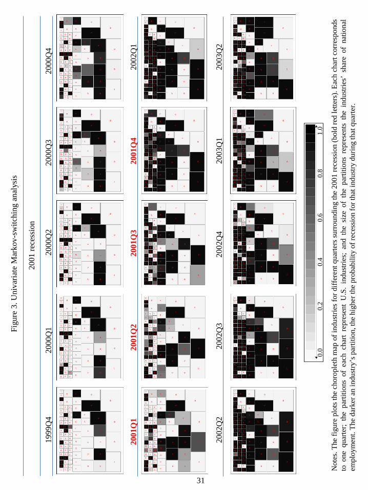
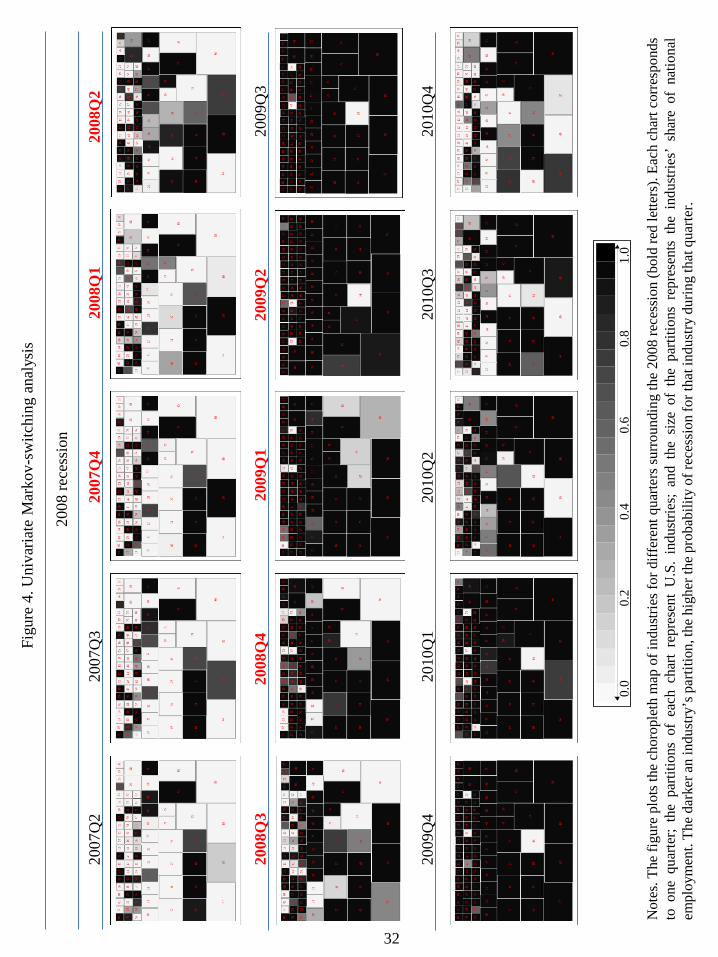
filtered probabilities of low-mean states, which appear in the choropleth maps displayed in
Figures 3 and 4.4 The charts are divided into rectangles that show the relative size of employment
in each of the 86 industries in the total.5 Light colours indicate low evidence of recession, while
the darker the shade, the stronger the statistical confidence that the indicated industry was in
recession at that time. As one moves to the right, the charts show how the business inferences
vary in each quarter, from pre-recession to recession and to the first stages of recovery, as dated
by the NBER.
Several conclusions emerge from the analysis of these choropleth charts. First, recessions are
marked by widespread contractions in many sectors of the economy. Second, goods-producing
industries, complementary businesses, and wholesale and retail industries are among the first
to fall at the onset of recessions. However, durable goods industries, professional and technical
services, businesses that operate facilities or that provide services to meet varied cultural, en-
tertainment and recreational interests, and industries providing transportation and warehousing
and storage for goods do not experience job cuts until some time after the beginning of re-
4To facilitate the exposition, the monthly figures have been converted to quarterly by averaging over the
respective quarter. The monthly analysis, available upon request, reveals qualitatively similar results.5To simplify the charts, we use the average relative size of industries over the sample period.
11

cessions. Third, businesses engaged in providing education and training, health care and social
assistance and industries providing utility services and public goods are less sensitive to national
recessions, especially to the 2001 recession.
3.3 Ergodic linkages
A glimpse of the business cycle linkages across the industries over the sample can be obtained
by collecting the pairwise ergodic probabilities of the Markov chain that governs the strength of
business cycle synchronization, vab,t, for all industries a, b. Therefore, we begin by calculating
the ergodic probabilities,
πabi =(
1− pabjj)/(
2− pab00 − pab11), (17)
that each industry pair exhibits independent (i = 0, j = 1) or perfectly synchronized (i = 1,
j = 0) cycles. Since the ergodic probabilities can be viewed as the unconditional probability
of each of the different states, the matrix of ergodic synchronizations provides insights on the
unconditional business cycle linkages across the industries. In this paper, we focus on the analysis
of business cycle distances, πab0 .
Although this approach is appealing, a diffi culty with it is that there are many such measures.
With a set of N industries, there are η = N (N − 1) /2 different possible business cycle distances.
It is therefore a challenge to organize and present the results in a coherent way. To overcome
this drawback, we take nonparametric density estimation approaches to examine the distribution
of the business cycle distances. These techniques allow us to provide complete information on
the entire distribution and have the advantage of letting the data speak for themselves. In this
framework, for a given bandwidth h, the kernel distribution of business cycle distances estimated
from the ergodic dissimilarities πab0 is
fh (π0) =1
ηh
N∑a=1
N∑b>a
K
(π0 − πab0
h
), (18)
where K (•) is the Gaussian kernel.
The density estimate of the cross-industry distributions of pairwise business cycle distances
is plotted in Figure 5. A preliminary inspection of the estimated density reveals that this is a
multimodal distribution, which shows at least two clear distinct local maxima. The left tail is
made up of industries that exhibit large degrees of business cycle synchronization (small dis-
tances), whereas the right tail is pretty much exclusively made up of industries with idiosyncratic
cycles (big distances). Although most of the distribution’s mass is located in the right tail, the
12
industries experiencing such idiosyncratic cycles tend to be smaller, in terms of total share of
U.S. employment, than the industries associated with the left tail, which experience high syn-
chronization. Between these two modes, one might detect a third peak, at around πab0 = 0.5.
The interpretation of this multimodality is that there is a mixed distribution containing two or
three subpopulations of industries with different degrees of business cycle synchronization.
The nonparametric density estimation approach enables us to explicitly test for the number
of modes of the underlying distribution. If confirmed, multimodality would point to population
heterogeneity, implying the existence of separate population groups. To test for multimodality,
we follow the lines suggested by Silverman (1981), who proposed a simple way to assess the p-
value that a density is at most k-modal against the alternative that it has more than m modes.
Since the number of modes in a normal kernel density estimate does not increase as h increases,
let hm be the minimum bandwidth for which the kernel density estimate is at most m-modal.
Let τab0 be a resample drawn from the estimated business cycle proximities
τab0 =(1 + h2m/s
2)−0.5 (
πab0 + hmuab), (19)
where s2 is the sample variance of the data, and uab is an independent sequence of standard
normal random variables. Let h∗m be the smallest possible h producing at most m modes in the
bootstrap density estimate
f∗h (τ0) =1
ηh
N∑a=1
N∑b>i
K
(π0 − τab0
h
). (20)
Repeated many times, the probability that the resulting critical bandwidths h∗m are larger than
hm, which is equivalent to the proportion of occurrences in which f∗hm (τ0) has more than m
modes, can be used as the p-value of the test.
Computed from 1, 000 replications, Table 2 displays the critical window widths and the
p-values of the null hypothesis that the underlying density has at most m modes against the
alternative that it has more than m modes, with m = 1, 2, 3, 4. The tests should be applied
successively for an increasing number of modes until, for a certain a number, the null is accepted.
Clearly, unimodality is rejected for all significance levels (p-value of 0.00), which suggests distinct
business cycle distribution dynamics for different population subgroups of industries. In addition,
the p-value corresponding to the null of bimodality versus trimodality is 0.27, which indicates
that the global distribution of ergodic business cycle distances is bimodal. It exhibits one hump
in the very low end representing the industries with a high level of business cycle synchronization
and then a larger hump representing those with idiosyncratic cycles.
13

Notably, the distribution shows a sizable concentration of mass in the middle range. This
could explain why the p-value for the test of three modes versus more than three modes falls
to 0.12, which is less conclusive. Using a significance level of 0.05, which is the most common
cut-off for p-values, the distribution is bimodal. However, using more conservative significance
levels, such as 0.15, the distribution would be trimodal (the p-value of four modes rises to 0.26).
Therefore, there are signals that the modes located at the tails of the distribution are not well
separated and the test does not exclude the possibility that the high-end range of the distribution
could be split into two subgroups.
Although useful, the kernel density estimation approach does not allow us to understand the
business cycle affi liations detected across the set of industries. To address this deficiency, we
employ clustering techniques and classical multi-dimensional scaling (see Timm, 2002, among
others) to the pairwise business cycle distances. Collecting the distances, πab0 , in the symmetric
matrix D, the goal of cluster analysis is to develop a classification scheme of our set of industries
in several distinct groups, since they present homogeneous business cycles. For this purpose,
we make use of dendograms, which are tree-structured graphs used to visualize the result of a
hierarchical clustering calculation. The end-points of the dendrogram depicted in Figure 6, whose
numbers appear in Table 1, represent the original industries. Clusters are successively combined,
forming the tree’s branches until the top of the graph. Although it is not easy to interpret,
the height of the tree represents the level of dissimilarity at which observations or clusters
are merged. Big jumps to join groups occur when there are high intergroup dissimilarities.
Therefore, a reasonable number of final groups is often obtained by cutting the dendogram at
those junctures. In line with the results obtained with the kernel approach, the dendogram
shows that two (cutting at around 2) or three (cutting at around 1.5) clusters could be enough
to explain the groups that form among the industries.
The multi-dimensional scaling map (see Appendix B) of business cycle similarities is reported
in Figure 7, whose plotted numbers refer to the industries listed in Table 1.6 Notably, the
industries grouped in the two/three different clusters of the dendogram belong to two/three
concentric circles, whose radius lengths reflect the business cycle dissimilarities from the centre
to the periphery. The U.S. economy appears in the centre or mass of the distribution of cyclical
similarities, reflecting that some industries seem to stick together in the map and show business
cycle experiences that are similar to those of the nation. Although they are a relatively small
6 In these maps, the axes are meaningless and the orientation of the picture is arbitrary.
14
number of industries, they represent 46.5% of total U.S. employment. However, the map also
shows an intermediary zone and a peripheral zone, indicating that other industries appear away
from the attractor and do not seem to be as closely related to the nation in terms of business
cycle as the industries at the core. The intermediary and peripherial zones are composed of
industries representing 20.6% and 32.9% of total employment, respectively.
Let us have a deeper look at these business cycle affi liations. The core, in which the to-
tal U.S. employment is also included to facilitate comparison, is plotted in the centre of the
map and includes goods-producing industries, which typically experience the largest declines in
unemployment during recessions (Bureau of Labor Statistics, 2012), such as construction and
textiles, wood, furniture, and electronic products manufacturers. According to Goodman and
Mance (2011), complementary businesses that may suffer from ripple effects, such as furniture
and food stores, accommodations, appraisal services, motor vehicles, parts manufacturing, and
rental and leasing services, are also included. Finally, this core is also formed by other procycli-
cal industries (Bureau of Labor Statistics, 2012), such as wholesale and retail trade and personal
services, support activities and business services, especially administrative and waste services.7
The contrast between the national business cycle attractor and those industries plotted in
the intermediary zone of the perceptual map is a telling indication of their lower (albeit some)
business cycle concordance. In this middle circle, we observe some manufacturing industries
that may be subject to labour hoarding. Although they depend on the national business cycle,
their synchronization could be diminished. According to Clark (1973), examples are durable
goods industries, such as chemical, rubber, plastic, primary metal and machinery manufactur-
ing, electrical equipment and building materials. In addition, Rotemberg and Summers (1990)
find that industries with a large ratio of nonproduction workers to employment also tend to
hoard labour.8 Examples are those businesses engaged in providing services in producing and
distributing information and cultural products and leisure activities. In addition, this cluster is
also formed by most of the industries providing transportation and related facilities, and ware-
housing and storage for goods. Interestingly, Christiano and Fitzgerald (1998) find that most of
the industries belonging to this cluster exhibit strong channels for intermediate goods.
The last cycle cluster is formed by some peripheral industries, which are less closely associ-
ated to the U.S. cycle. These industries are plotted further away from the business cycle centre,
7Conlon (2011) documented that the payrolls of administrative and waste services shrank by more than 1
million positions during the Great Recession.8Parsons (1986) also documented a stronger tendency to hoard nonproduction labour.
15

which reflects their low sensitivity to the national cycle. In addition, they appear separate from
each other, which indicates that their business cycle shocks are idiosyncratic. This cluster is
mainly formed by those industries classified by Berman and Pfleeger (1997) as “not coinciden-
tally cyclical” industries. For some of these industries, the consequences of a negative demand
shock are relatively reduced since their product cannot normally be postponed. Examples are
businesses engaged in providing education and training, health care and social assistance, and
industries providing utility services, such as electric power, natural gas, steam supply, water
supply and sewage removal.9
In addition, this cluster includes sectors that depend highly on international shocks, such
as mineral extraction and its related supporting activities, as well as gasoline stations, or on
international competition, such as wholesale electronic markets.10 Also belonging to this cluster
are industries providing financial services, not because they are not cyclical, but because they
typically lead the national cycle.11 Finally, we find in this cluster monetary authorities, and
federal, state and local government services. These industries provide necessities or public
goods and demand for these goods remains relatively strong throughout lows in the economy.
3.4 Evolution of linkages
How have industrial business cycle linkages evolved over time? Traditionally, the literature
would address this question by dividing a full sample into several sub-periods. The problem
with this approach is that it would provide pictures of the cycle linkages that rely on specific
date breaks, the location of which is sometimes controversial. To overcome this drawback, the
pairwise probabilities of cycle dependence p (vab,t = i) for all industries a, b, are collected for
all periods t. Kernel density estimates, multimodality tests and multi-dimensional scaling maps
can then be calculated for each month of the sample. Accordingly, the pictures of Kernel density
and multi-dimensional scaling become animated videos that allow one to easily identify which
industries manifested the first signs of phase changes and to examine how the interconnections
9Goodman (2001) finds that private education and health care services are countercyclical. In fact, employment
in these industries has decreased in only 1 of the 12 NBER recessions that have occurred since 1945 (Bureau of
Labor Statistics, 2012).10Groshen and Potter (2003) find that oil and gas extraction firms are countercyclical.11Christiano and Fitzgerald (1998) find that the business cycle components of the finance, insurance and real
estate industries exhibit low contemporaneous co-movement with aggregate employment. Goodman and Mance
(2011) show that employment in financial activities peaked one year before the offi cial start of the Great Recession.
16

among industries propagate the business cycle shocks across industries.12
To examine the intra-distribution evolution of business cycle proximities, Figure 8 and Fig-
ure 9 plot the overlaid families of empirical kernel distributions across several months around
the 2001 and 2008 recessions, respectively. When interpreting these charts, it is worth empha-
sizing that the horizontal axis measures pairwise business cycle dissimilarities. Therefore, each
right-hand horizontal movement represents absolute losses in pairwise synchronization among
industries.
Figure 8 shows that in some months before the 2001 recession, the densities exhibited a tri-
modal distribution of business cycle distances, agreeing with the pattern obtained in the multi-
dimensional scaling analysis. That is, we find a core composed of industries highly synchronized
with each other (left-hand mode), a group of moderately synchronized industries (middle mode)
and some idiosyncratic industries that follow independent cyclical patterns (right-hand mode).
However, as the economy approached the recession, the distribution tended to reshape to bi-
modal. This occurred because industries did not fall into the recession simultaneously but
sequentially, as indicated in Figure 3. The first industries to fall into the recession were those
in the core, while the industries that belonged to the middle mass remained in expansion. This
reduced the synchronization and pushed the middle mass of the distribution to the right-hand
side.
During the recession, more industries changed the phase cycle, which implied that a third
mode appeared again in the middle of the distribution. However, when the trough took place,
the cyclical position was reversed back. The core changed the phase cycle first, accentuating the
business cycle discrepances with the middle mass, which shifted again to the right. Therefore, the
distribution was reshaped to bimodal as it did in the peak. Finally, the middle mode appeared
again when more industries initiated the recovery phase after the core.
A similar but more accentuated pattern occurred during the 2008 recession. Figure 9 shows
that before the recession, the distribution seemed to be characterized by three modes. When the
peak occurred, the distribution became bimodal, since industries fell into recession sequentially,
providing evidence of a cascade effect. Once the economy was in recession, the trimodal pattern
in the distribution was recovered until the peak, when only the industries in the core initiated
the recovery and the distribution became bimodal again. The cycle ended when the economy
returned to the stable expansionary phase, and the distribution presented three modes, which
12 The full animated graphs for this paper can be found at http://www.um.es/econometria/Maximo.
17
remained until the next turning point.
In sum, we find that the propagation of micro-level shocks to national shocks is enhanced
when the mass shifts that characterize the turning points occur. A formal statistical test of this
pattern is provided by applying the modality tests in the density distributions of business cycle
similarities from January 1991 to May 2013. According to the plots of the kernel densities, the
nulls of unimodality (not shown here to save space) were clearly rejected for all months, since the
p-values were always quite close to zero. Figure 10 plots the p-values of the null of two versus
more than two modes. To facilitate the analysis, the figure includes shaded areas that refer
to the NBER-referenced recessions and a dashed line that refers to the 0.05 significance level.
The figure shows that bimodality is rejected during national expansions and recessions while it
cannot be rejected at any reasonable level of significance at the turning points.13 Notably, the
lagged business cycle behaviour that characterizes employment implies that bimodality appears
with some lags with respect to the NBER turning points. Therefore, the Silverman test confirms
the mass shift in turning points documented above. In other words, the time-varying p-values
reaching the 0.05 threshold could be interpreted as indicators of national turning points in
(employment) cycles.
Which industries are involved in these large changes in the distribution? To address this
question, Figure 11 captures the polarization tendencies around turning points documented in
the density estimate analysis. For this purpose, the figure shows three representative months out
of the 269 multi-dimensional scaling maps computed in our sample period. Following the NBER
classification, the maps capture the across-industry business cycle distances in an expansion,
June 2000, and in a recesison, March 2009. In both cases, the maps refer to months for which the
modality test detected trimodal distributions. The figure also shows the map dated September
2002, which is a month in which the modality test detected only two modes.
The within-expansion and within-recession maps look similar to the map computed from
the ergodic probabilities. According to their corresponding trimodal distributions of business
cycle distances, they show concentric circles of industries that exhibit highly, moderately and
lowly synchronized cycles with each other and with the national business cycle. However, the
map that refers to the period of transition from an expansion to a recession reflects a higher
dispersion across industries, which agrees with a bimodal distribution of business cycle distances.
According to this figure, it appears that the polarization could be owing to the fact that some
13Although it is not shown to save space, when bimodality is rejected, trimodality could not be rejected.
18

industries in the core were engaged in an expansionary phase, while others in the core and the
middle circle continued in a contractionary phase.
Let us focus on peaks since troughs behave symmetrically. The movements that occurred
during the transitions are initiated by some industries that are in the core and many industries
that are in the middle mass, which did not experience the severe job losses that the core did in
the initial stages of the recessions. Over the course of the national downturns, these industries
start to experience the deepening of the economic downturns and the pace of declines accel-
erated as employment losses spread to them. Among these industries, we find durable goods
industries, private services industries, professional and technical services, recreational services,
and industries providing transportation, warehousing and storage for goods.
These industries fall when there is no way back in a national recession, clearly indicating a
phase shift. We postulate that this salient characteristic of peaks could be caused by at least
one of the following determinants. First, since investments in durable goods can usually be
postponed, buyers can benefit from waiting to receive more information about how the economy
develops. Therefore, the contagion appears only when the recession becomes more evident.
Second, although labour hoarding guarantees that employee talent will be available, the practice
implies high risks, since it reduces companies’profitability during diffi cult times. When the bad
times are prolonged, their negative consequences become unavoidable. Third, some of the output
of the consumption goods sector, which is in the core, is also used as intermediate goods in the
production of durable goods, such as machinery and equipment, which are in the middle mass.
During the recession, the durable goods industries are seriously exposed to ripple effects, which
come from the core with some lags.
4 Concluding remarks
This paper is part of a growing empirical literature that analyzes the sources of interindustry
co-movements. It differs from this literature in several respects. First, the approach is in the
mould of “measurement without theory”. Using employment data, we ask whether industry-
level business cycles are coherent not only with the national business cycle, but also with each
other. Second, the filter used to compute the business cycle inferences is an extension of the
Markov-switching filter that allows for time-varying business cycle interdependence. Third,
nonparametric density estimation techniques are applied to assess the degree of population het-
19

erogeneity and to examine the changes in the business cycle distribution. Finally, heuristic
techniques of classical multi-dimensional scaling and clustering are used to understand the in-
dustry movements going in and out of recessions, which helps us to identify changes in cyclical
affi liations.
Our main results are the following. First, there is a large heterogeneity in the distribution
of business cycle similarities, implying the existence of population groups that follow distinct
distributional dynamics. Second, there is not a monotone movement toward the emergence of
an increasingly cohesive national business cycle core. The positions of the lower mode, which
comprises extremely synchronized industries, and the cluster at the high end of the distribution,
which represents industries with idiosyncratic cycles, are relatively stable over time. However,
the position of a third, middle mode when the economy is in expansionary or recessionary phases
jumps up substantially during the period of transition from one phase to another, switching
from pairwise business cycle distances of just over 0.5 to almost one. Therefore, the proposed
framework is able to provide assessments of when a national turning point takes place and how
the business cycle shocks propagate across industries.
The model used in this paper provides a solid foundation for starting a line of research that
seeks to explain the determinants of the business cycle affi liations across industries. Various
factors have been put forward in the literature that may affect business cycle synchronization,
ranging from the proportion of fixed and variable costs, industry concentration, product differ-
entiation and dependence on external finance. However, the modifications of the model used in
the paper to capture the changes in affi liations would be substantial; therefore, this task is left
to future research.
20

Appendix AThis appendix describes the estimation of the parameters in vector θ and the inference on
s∗ab,T , which is performed through a multi-move Gibbs-sampling procedure. The distribution
of the parameters can be approximated by the empirical distributions of simulated values, by
iterating the following steps.
STEP 1. The Gibbs sampler is started with arbitrary starting values for the parameters of
the model, θ0, which are used to generate s∗1ab,T |yab,T , θ0. For this purpose, we run the Markov-
switching filter described in Section 2 and obtain the filtered probabilities p(s∗ab,t|yab,t, θ0). To
draw the state variables, we employ the following result:
p(s∗ab,T |yab,T , θ0
)= p
(s∗ab,T |yab,T , θ0
) T−1∏t=1
p(s∗ab,t|s∗ab,t+1, yab,t, θ0). (A1)
The last iteration of the Markov-switching filter provides us with p(s∗ab,T |yab,T , θ
0), from which
s∗ab,T is generated. To generate s∗ab,t, with t = 1, ..., T − 1, we use
p(s∗ab,t|s∗ab,t+1, yab,t, θ0) = p(s∗ab,t+1|s∗ab,t) ∝ p(s∗ab,t|yab,t, θ0), (A2)
where p(s∗ab,t|s∗ab,t+1) refers to the transition probabilities, which are included in θ0. Using this
expression, it is straightforward to generate s∗ab,t by computing the probability of state i from
p(s∗ab,t = i|s∗ab,t+1, yab,t, θ0) =p(s∗ab,t+1|s∗ab,t = i)p(s∗ab,t = i|yab,t, θ0)∑
j 6=ip(s∗ab,t+1|s∗ab,t = j)p(s∗ab,t = j|yab,t, θ0)
. (A3)
Using random numbers from a uniform distribution between 0 and 1, s∗1ab,t is set to a par-
ticular state i by comparing the probability of this state with the random numbers. Follow-
ing a similar reasoning, one can also generate s1k,T = s1k,1, ..., s1k,T , v
1ab,T = v1ab,1, ..., v
1ab,T and
ς1ab,T = ς1ab,1, ..., ς1ab,T , for any industry k and any pair a and b at any time t = 1, ..., T .
STEP 2. The generated state variables are used to draw the transition probabilities pkij , pabij
and qabij . Since these parameters are drawn in a similar way, we focus only on pkij to save space.
Conditional on sk,T , the transition probabilities are independent of the data set yab,T and the
model’s other parameters. Given s1k,T , let nkij , i, j = 0, 1 be the total number of transitions from
state i to state j in industry k. By taking the beta family of distributions as conjugate priors,
pkii˜beta(ukii, ukij), (A4)
21
where ukii and ukij are known parameters of the priors, it can be shown that the posterior
distributions of pkii are given by
pkii|sk,T , yab,T ˜beta(ukii + nkii, ukij + nkij), (A5)
from which pk1ii is drawn. In particular, we set uk00 = 8, uk01 = 2, uk11 = 0 and uk10 = 1 for all k.
STEP 3. Conditional on the covariance matrix Ωab, the generated state variables and tran-
sition probabilities are used to draw the means. Let µab = (µa0, µa1, µb0, µb1)′ be the vector of
means for which we assume a normal prior,
µab˜N(µ∗ab, V∗ab), (A6)
where the expected values µ∗ab and the covariance matrix V∗ab are known. The model can now
be expressed as
ya,t
yb,t
=
1
0
sa,t
0
0
1
0
sb,t
µa0
µa1
µb0
µb1
+
εa,t
εb,t
, (A7)
or
yab,t = Dab,tµab + εab,t, (A8)
with εab,t˜N(0,Ωab). According to the large business cycle heterogeneity across industries doc-
umented in the empirical analysis, we estimate the univariate models by maximum likelihood
and use the estimated state-dependent means to specify the parameters µ∗ab of the priors. To
check for robustness, we also tried with µi0 = ymini and µi1 = ymaxi − ymini , where ymini and ymaxi
are the minimum and maximum values of employment growth in the ith industry, with i = a, b,
but the results were unchanged. For the covariance matrices, we set V ∗ab = I for all a, b.
The posterior distribution of µab is given by
µab|s∗1ab,T , yab,T ,Ωab˜N(µ+ab, V+ab ), (A10)
where
V +ab =
(V ∗−1ab +
T∑t=1
D′ab,tΩ−1ab Dab,t
)−1, (A11)
µ+ab = V +ab
(V ∗−1ab µ∗ab +
T∑t=1
D′ab,tΩ−1ab Dab,t
). (A12)
22
STEP 4. Conditional on the generated state variables, transition probabilities and state-
dependent means, the parameters of the covariance matrix are drawn. For this purpose, we use
the Wishart distribution as the conjugate prior of the inverse covariance matrix,
Ω−1ab ∼W (Σ∗−1ab , r∗ab), (A13)
where Σ∗ab and r∗ab are known. In particular, we set Σ∗ab = I and r∗ab = 0. Then, the posterior
distribution is
Ω−1ab |s∗1ab,T , yab,T , µ
1ab ∼W (Σ+−1ab , r+ab), (A14)
where
r+ab = T + r∗ab, (A15)
Σ+−1ab = Σ∗−1ab +
T∑t=1
(yab,t −D1
ab,tµ1ab
) (yab,t −D1
ab,tµ1ab
)′. (A16)
Steps 1 through 4 can be iterated L+M times, where L is large enough to ensure that the
Gibbs sampler has converged. Thus, the marginal distributions of the state variables and the
parameters of the model can be approximated by the empirical distribution of the M simulated
values.
Appendix BThis appendix describes the main steps followed to compute dendograms and multi-dimensional
scaling maps. Detailed descriptions of these methods can be found in Timm (2002).
To compute the dendograms, we begin the analysis with N (N − 1) /2 clusters, each con-
taining only one industry. Using the matrix of business cycle distances, D = [dij ], the algorithm
searches for the “most similar” pairs of industries, so that industry a and b are selected. In
this respect, we follow the most similar criterion that is based on the minimum increase in the
within-group variance of distances. Industries a and b are now combined into a new cluster,
called p, which reduces the total number of clusters by one. Then, dissimilarities between the
new cluster and the remaining clusters are computed again following the most similar criterion.
For instance, the distance from the new cluster p to, say, industry q, is computed according to
dp,q =na + nqnp + nq
da,q +nb + nqnp + nq
db,q −nq
np + nqda,b, (B1)
where na, nb, np and nq are the number of industries included in the respective clusters, and
da,b, da,q, and db,q are the business cycle distances. Finally, these steps are repeated until all
industries form a single cluster.
23

The second classification technique used in this paper is multi-dimensional scaling. To com-
pute these maps, we project the business cycle distances among the N industries in a map in
such a way that the Euclidean distances among the industries plotted in the plane approximate
the business cycle dissimilarities. In the resulting map, industries that exhibit large business
cycle dissimilarities have representations in the plane that are far away from each other. Given
the matrix of business cycle distances, D, the technique searches the the so-called (N × 2) con-
figuration matrix X that contains the position in two orthogonal axes to which each industry is
placed in the map. Following Timm (2002), we define
B =1
2
(I −N−1O
)D2(I −N−1O
), (B2)
where I is the identity matrix and O is a (N ×N) of ones. We then compute the (2× 2) diagonal
matrix Λ with the two largest eigenvalues of B on the main diagonal, and P , the (N × 2) matrix
of its corresponding eigenvectors. The classical metric scaling coordinates correspond to
X = PΛ1/2. (B3)
24
References
[1] Acemoglu, D., V. Carvalho, A. Ozdaglar, and A. Tahbaz-Salehi (2012), The network origins
of aggregate fluctuations. Econometrica 80: 1977-2016.
[2] Barker, M. (2011), Manufacturing employment hard hit during the 2007—09 recession.
Monthly Labor Review, April: 28-33.
[3] Bengoechea, P., M. Camacho, and G. Perez Quiros (2006), A useful tool for forecasting the
Euro-area business cycle phases. International Journal of Forecasting 22: 735-749.
[4] Berman, J. and J. Pfleeger (1997), Which industries are sensitive to business cycles?
Monthly Labor Review, February: 19-25.
[5] Bureau of Labor Statistics (2012), The recession of 2007-2009. BLS Spotlight on Statistics,
February.
[6] Camacho, M., and G. Perez Quiros (2006), A new framework to analyze business cycle
synchronization. In: Milas, C., Rothman, P., and van Dijk, D. Nonlinear Time Series
Analysis of Business Cycles. Elsevier’s Contributions to Economic Analysis series. Chapter
5 (pp. 133-149). Elsevier, Amsterdam.
[7] Carlino, G., R. H. DeFina (2004), How strong is co-movement in employment over the
business cycle? Evidence from state/industry data. Journal of Urban Economics 55: 298-
315.
[8] Christiano, L., and T. Fitzgerald (1998), The business cycle: it’s still a puzzle. Economic
Perspectives, Fourth Quarter: 56-83.
[9] Clark, S. (1973), Labor hoarding in durable goods industries. American Economic Review
63: 811-824.
[10] Conlon. F. (2011), Professional and business services: employment trends in the 2007-09
recession. Monthly Labor Review April: 34-39.
[11] Filardo, A. (1997), Cyclical implications of the declining manufacturing employment share.
Federal Reserve Bank of Kansas City Economic Review II: 63-87.
25
[12] Foerster, A., P. Sarte, and M. Watson (2011), Sectorial versus aggregate shocks: a structural
factor analysis of industrial production. Journal of Political Economy 119: 1-38.
[13] Gabaix, X. (2011), The granular origins of aggregate fluctuations. Econometrica 79: 733-
772.
[14] Goodman, W. (2001), Employment in services industries affected by recessions and expan-
sions. Monthly Labor Review October: 3-11.
[15] Goodman, W., and S. Mance (2011), Employment loss and the 2007-09 recession: an
overview. Monthly Labor Review April: 3-12.
[16] Groshen, E., and S. Potter (2003), Has structural change contributed to a jobless recovery?
Current Issues in Economics and Finance 9 (August).
[17] Hamilton, J. (1989), A new approach to the economic analysis of nonstationary time series
and the business cycles. Econometrica 57: 357-384.
[18] Hamilton, J., and M. Owyang (2012), The Propagation of Regional Recessions. The Review
of Economics and Statistics, 94(4): 935—947.
[19] Leiva-Leon, D. (2014), A New Approach to Infer Changes in the Synchronization of Business
Cycle Phases. Working Paper, Bank of Canada, 2014-38.
[20] Malmendier, U., and S. Nagel (2011), Depression babies: Do macroeconomic experiences
affect risk taking? The Quarterly Journal of Economics 126: 373-416.
[21] Owyang, M., J. Piger, and H. Wall (2005), Business cycle phases in the U.S. states. The
Review of Economics and Statistics 87: 604-616.
[22] Owyang, M., J. Piger, H. Wall, and C. Wheeler (2008), The economic performance of cities:
A Markov-switching approach. Journal of Urban Economics 64: 538-550.
[23] Parsons O. (1986), The employment relationship: Job attachment, work effort and the
nature of contracts. Handbook of Labor Economics. Ashenfelter O, Layard R (eds.), Elsevier:
New York.
[24] Peterson, B., and S. Strongin (1996), Why are some industries more cyclical than others?
Journal of Business and Economic Statistics 14(2) : 189-198.
26

[25] Phillips, K. (1991), A two-country model of stochastic output with changes in regime.
Journal of International Economics, 31 (1-2) 121-142.
[26] Rotemberg J, and L. Summers (1990), Inflexible Prices and Procyclical productivity. Quar-
terly Journal of Economics 105: 851-874.
[27] Silverman, B. (1981), Using kernel density estimates to investigate multimodality. Journal
of the Royal Statistical Society, Series B 43: 97-99.
[28] Timm, N. (2002), Applied multivariate analysis. Springer texts in Statistics.
[29] Urquhart, M. (1981), The services industry: Is it recession-proof? Monthly Labor Review
October: 12-18.
27
28
Table 1. Properties of the sectorial business cycles
Industry, 3 digits Averaged growth rates Total Expansion Recession
Forestry (1) -2.17 -1.52 -7.60 Oil and Gas Extraction (2) 0.15 -0.38 4.58 Mining, except Oil and Gas (3) -1.26 -1.23 -1.53 Support Activities for Mining (4) 4.03 3.74 6.39 Construction of Buildings (5) -0.35 0.62 -8.38 Heavy and Civil Engineering Construction (6) 0.47 1.02 -4.10 Specialty Trade Contractors (7) 0.93 1.79 -6.18 Food Manufacturing (8) -0.10 -0.05 -0.44 Textile Mills (9) -6.08 -5.30 -12.51 Textile Product Mills (10) -3.01 -2.40 -8.02 Apparel Manufacturing (11) -7.66 -7.26 -10.96 Wood Product Manufacturing (12) -1.83 -0.58 -12.20 Paper Manufacturing (13) -2.35 -2.10 -4.37 Printing and Related Support Activities (14) -2.45 -2.04 -5.79 Petroleum and Coal Products Manufacturing (15) -1.27 -1.49 0.51 Chemical Manufacturing (16) -1.20 -1.05 -2.48 Plastics and Rubber Products Manufacturing (17) -0.96 -0.29 -6.48 Nonmetallic Mineral Product Manufacturing (18) -1.55 -0.84 -7.42 Primary Metal Manufacturing (19) -2.23 -1.59 -7.56 Fabricated Metal Product Manufacturing (20) -0.43 0.17 -5.35 Machinery Manufacturing (21) -0.96 -0.54 -4.42 Computer and Electronic Product Manufacturing (22) -2.35 -2.11 -4.34 Electrical Equipment, Appliance, and Component Manufacturing (23) -2.30 -1.96 -5.06
Transportation Equipment Manufacturing (24) -1.52 -0.71 -8.20 Furniture and Related Product Manufacturing (25) -2.21 -1.18 -10.71 Miscellaneous Manufacturing (26) -1.98 -1.90 -2.64 Merchant Wholesalers, Durable Goods (27) 0.07 0.54 -3.78 Merchant Wholesalers, Nondurable Goods (28) 0.21 0.43 -1.61 Wholesale Electronic Markets and Agents and Brokers (29) 2.28 2.63 -0.55 Motor Vehicle and Parts Dealers (30) 0.76 1.41 -4.58 Furniture and Home Furnishings Stores (31) 0.27 1.19 -7.39 Electronics and Appliance Stores (32) 0.63 1.18 -3.94 Building Material and Garden Equipment and Supplies Dealers (33) 1.29 1.88 -3.61
Food and Beverage Stores (34) 0.17 0.23 -0.36 Health and Personal Care Stores (35) 1.13 1.20 0.56 Gasoline Stations (36) -0.31 -0.12 -1.95 Clothing and Clothing Accessories Stores (37) 0.42 0.81 -2.80 Sporting Goods, Hobby, Book, and Music Stores (38) 1.05 1.29 -0.91 General Merchandise Stores (39) 0.97 1.14 -0.40 Miscellaneous Store Retailers (40) 0.46 0.90 -3.16 Nonstore Retailers (41) 0.31 0.61 -2.14 Air Transportation (42) -0.62 -0.55 -1.16 Rail Transportation (43) -0.68 -0.47 -2.43 Water Transportation(44) 0.55 0.73 -0.89 Truck Transportation (45) 0.94 1.52 -3.82 Transit and Ground Passenger Transportation (46) 2.34 2.42 1.68 Pipeline Transportation (47) -1.27 -1.70 2.31 Scenic and Sightseeing Transportation (48) 2.59 2.79 1.00 Support Activities for Transportation (49) 2.18 2.46 -0.12 Couriers and Messengers (50) 1.69 2.19 -2.44
29
Warehousing and Storage (51) 2.41 2.80 -0.75 Utilities (52) -1.26 -1.48 0.55 Publishing Industries, except Internet (53) -0.71 -0.40 -3.23 Motion Picture and Sound Recording Industries (54) 1.93 2.47 -2.50 Broadcasting, except Internet (55) 0.05 0.27 -1.73 Telecommunications (56) -0.59 -0.53 -1.07 Data Processing, Hosting, and Related Services (57) 0.85 1.24 -2.37 Other Information Services (58) 5.54 6.11 0.84 Monetary Authorities - Central Bank (59) -1.47 -1.73 0.76 Credit Intermediation and Related Activities (60) 0.34 0.69 -2.56 Securities, Commodity Contracts, and Other Financial Investments and Related Activities (61) 2.73 3.04 0.22
Insurance Carriers and Related Activities (62) 0.69 0.71 0.47 Funds, Trusts, and Other Financial Vehicles (63) 2.24 2.22 2.33 Real Estate (64) 1.14 1.35 -0.59 Rental and Leasing Services (65) 0.10 0.59 -3.95 Lessors of Nonfinancial Intangible Assets, except Copyrighted Works (66) 2.58 2.94 -0.43
Professional, Scientific, and Technical Services (67) 2.60 2.83 0.66 Management of Companies and Enterprises (68) 0.89 0.98 0.11 Administrative and Support Services (69) 2.69 3.76 -6.16 Waste Management and Remediation Services (70) 2.24 2.47 0.32 Educational Services (71) 3.14 3.06 3.77 Ambulatory Health Care Services (72) 3.70 3.74 3.42 Hospitals (73) 1.42 1.30 2.40 Nursing and Residential Care Facilities (74) 2.47 2.41 2.97 Social Assistance (75) 4.16 4.22 3.67 Performing Arts, Spectator Sports, and Related Industries (76) 1.94 2.20 -0.25 Museums, Historical Sites, and Similar Institutions (77) 3.20 3.39 1.62 Amusement, Gambling, and Recreation Industries (78) 2.73 3.03 0.20 Accommodation (79) 0.57 0.89 -2.07 Food Services and Drinking Places (80) 1.97 2.19 0.14 Repair and Maintenance (81) 0.80 1.20 -2.45 Personal and Laundry Services (82) 0.76 0.85 0.03 Religious, Grantmaking, Civic, Professional, and Similar Organizations (83) 1.46 1.45 1.53
Federal Government (84) -0.55 -0.58 -0.30 State Government (85) 0.72 0.62 1.55 Local Government (86) 1.14 1.09 1.54 United States 0.94 1.20 -1.23
Notes. Industries by NAICS Code. Numbers with which they appear in multi-dimensional scaling maps are in brackets. The last three columns refer to the average growth rate of employment (total, within the NBER expansions and within the NBER recessions). The shading pattern refers to the classification of industries at two digits.
Table 2. Bootstrap multimodality tests
N. modes under null
Critical bandwith p-value
1 0.141 0.00
2 0.031 0.27 3 0.028 0.12
4 0.021 0.26 Notes. Each row shows the number of modes under the null, the critical bandwidth and the corresponding p-value of the Silverman (1981) test.
Figu
re 1
. U.S
. em
ploy
men
t
Not
es. T
he fi
gure
plo
ts a
nnua
l gro
wth
rate
s. Sh
aded
are
as in
dica
te N
BER
rece
ssio
ns.
Figu
re 2
. Ker
nel d
istri
butio
n ov
er th
e cy
cle
Not
es. T
he fi
gure
plo
ts th
e ke
rnel
dis
tribu
tion
of y
ear-o
ver-
year
em
ploy
men
t gro
wth
acr
oss i
ndus
tries
. Exp
ansi
ons a
nd re
cess
ions
ar
e ob
tain
ed fr
om th
e N
BER
bus
ines
s cyc
le d
ates
.
.00
.04
.08
.12
.16
.20
-16
-14
-12
-10
-8-6
-4-2
02
46
81
0
Density
Rec
essi
on
Expa
nsio
n
-6-4-2024 19
91
.01
19
95
.06
19
99
.11
20
04
.04
20
08
.09
20
13
.02
30
Figu
re 3
. Uni
varia
te M
arko
v-sw
itchi
ng a
naly
sis
Not
es. T
he fi
gure
plo
ts th
e ch
orop
leth
map
of i
ndus
tries
for d
iffer
ent q
uarte
rs su
rroun
ding
the
2001
rece
ssio
n (b
old
red
lette
rs).
Each
cha
rt co
rres
pond
s to
one
qua
rter;
the
parti
tions
of
each
cha
rt re
pres
ent
U.S
. in
dustr
ies;
and
the
siz
e of
the
par
titio
ns r
epre
sent
s th
e in
dustr
ies’
sha
re o
f na
tiona
l em
ploy
men
t. Th
e da
rker
an
indu
stry
’s p
artit
ion,
the
high
er th
e pr
obab
ility
of r
eces
sion
for t
hat i
ndus
try d
urin
g th
at q
uarte
r.
2001
rece
ssio
n
199
9Q4
2000
Q1
2
000Q
2
20
00Q
3
2
000Q
4
200
1Q1
200
1Q2
200
1Q3
200
1Q4
200
2Q1
200
2Q2
200
2Q3
200
2Q4
200
3Q1
200
3Q2
31
0.0
0.2
0.
4
0
.6
0.8
1.0
Figu
re 4
. Uni
varia
te M
arko
v-sw
itchi
ng a
naly
sis
200
7Q2
200
7Q3
200
7Q4
200
8Q1
2008
Q2
200
8Q3
200
8Q4
200
9Q1
200
9Q2
200
9Q3
200
9Q4
201
0Q1
201
0Q2
201
0Q3
201
0Q4
2008
rece
ssio
n
32
Not
es. T
he fi
gure
plo
ts th
e ch
orop
leth
map
of i
ndus
tries
for d
iffer
ent q
uarte
rs su
rroun
ding
the
2008
rece
ssio
n (b
old
red
lette
rs).
Each
cha
rt co
rres
pond
s to
one
qua
rter;
the
parti
tions
of
each
cha
rt re
pres
ent
U.S
. in
dustr
ies;
and
the
siz
e of
the
par
titio
ns r
epre
sent
s th
e in
dustr
ies’
sha
re o
f na
tiona
l em
ploy
men
t. Th
e da
rker
an
indu
stry
’s p
artit
ion,
the
high
er th
e pr
obab
ility
of r
eces
sion
for t
hat i
ndus
try d
urin
g th
at q
uarte
r.
0.0
0.2
0.
4
0
.6
0.8
1.0

Figu
re 5
. Ker
nel d
ensi
ty e
stim
atio
n fr
om e
rgod
ic p
roba
bilit
ies
Not
es. D
ensi
ty e
stim
ates
of t
he c
ross
-indu
stry
dis
tribu
tions
of p
airw
ise
busi
ness
cyc
le s
ynch
roni
zatio
n us
ing
ergo
dic
prob
abili
ties.
33

Figu
re 6
. Clu
ster
ana
lysi
s w
ith e
rgod
ic p
roba
bilit
ies
Not
es.
The
dend
ogra
m’s
hei
ghts
rep
rese
nt t
he l
evel
of
diss
imila
rity
at w
hich
obs
erva
tions
or
clus
ters
are
mer
ged.
Num
bers
use
d to
re
pres
ent t
he in
dust
ries a
re p
rovi
ded
in T
able
1.
1453
4578
6 7
5570
8119
2750
6920
7938
5167
US82
2223
4132
6140
49 5
2810
6465
1218
3325
3037
3180
117
26 9
1311
1624
343
2168
2 4
1547
52 8
3577
2954
3436
3984
4476
4642
5657
5848
5985
7375
8660
6263
6671
8372
740
0.51
1.52
34
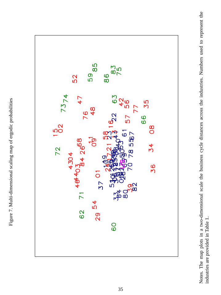
Figu
re 7
. Mul
ti-di
men
sion
al s
calin
g m
ap o
f erg
odic
pro
babi
litie
s
Not
es.
The
map
plo
ts i
n a
two-
dim
ensi
onal
sca
le t
he b
usin
ess
cycl
e di
stan
ces
acro
ss t
he i
ndus
tries
. N
umbe
rs u
sed
to r
epre
sent
the
in
dust
ries a
re p
rovi
ded
in T
able
1.
35
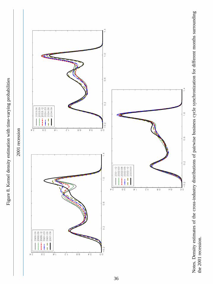
Figu
re 8
. Ker
nel d
ensi
ty e
stim
atio
n w
ith ti
me-
vary
ing
prob
abili
ties
Not
es. D
ensi
ty e
stim
ates
of t
he c
ross
-indu
stry
dis
tribu
tions
of p
airw
ise
busi
ness
cyc
le s
ynch
roni
zatio
n fo
r diff
eren
t mon
ths
surr
ound
ing
the
2001
rece
ssio
n.
2001
rece
ssio
n
36
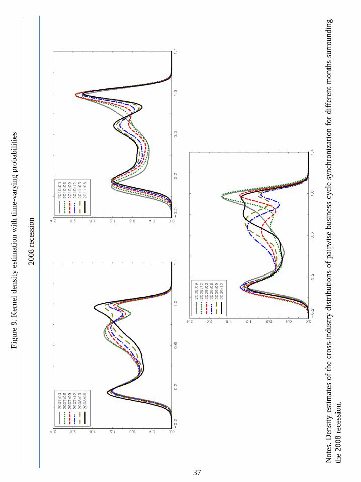
Not
es. D
ensi
ty e
stim
ates
of t
he c
ross
-indu
stry
dis
tribu
tions
of p
airw
ise
busi
ness
cyc
le s
ynch
roni
zatio
n fo
r diff
eren
t mon
ths
surr
ound
ing
the
2008
rece
ssio
n.
Figu
re 9
. Ker
nel d
ensi
ty e
stim
atio
n w
ith ti
me-
vary
ing
prob
abili
ties
2008
rece
ssio
n
37
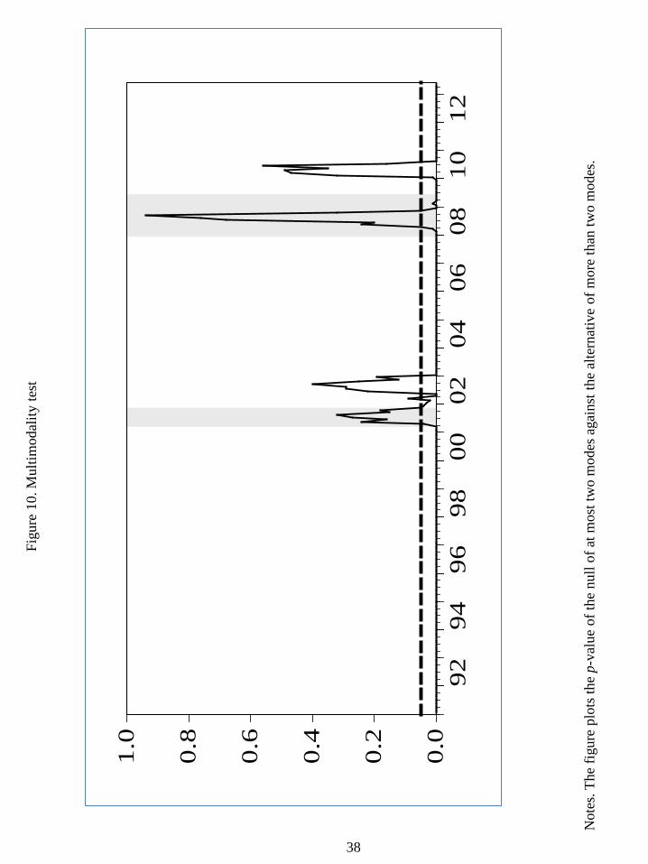
Figu
re 1
0. M
ultim
odal
ity te
st
Not
es. T
he fi
gure
plo
ts th
e p-
valu
e of
the
null
of a
t mos
t tw
o m
odes
aga
inst
the
alte
rnat
ive
of m
ore
than
two
mod
es.
0.0
0.2
0.4
0.6
0.8
1.0
9294
9698
0002
0406
0810
12
38
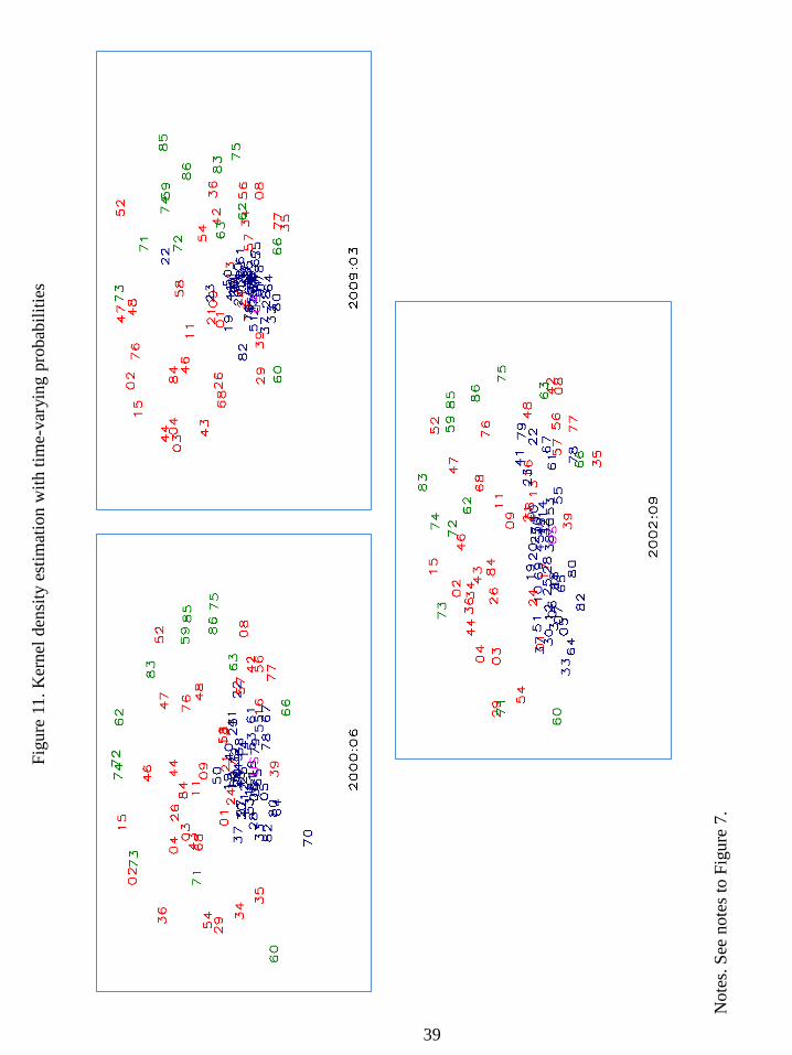
Figu
re 1
1. K
erne
l den
sity
est
imat
ion
with
tim
e-va
ryin
g pr
obab
ilitie
s
Not
es. S
ee n
otes
to F
igur
e 7.
39