Embed Size (px)
Citation preview
The Proof of Lin’s Conjecture via the Decimation-Hadamard
Transform
1Honggang Hu, 1Shuai Shao, 2Guang Gong, and 3Tor Helleseth
1School of Information Science and Technology
University of Science and Technology of China
Hefei, China, 230027
Email. [email protected]
2Department of Electrical and Computer Engineering
University of Waterloo
Waterloo, Ontario N2L 3G1, Canada
Email. [email protected]
3The Selmer Center
Department of Informatics
University of Bergen
PB 7803, N-5020 Bergen, Norway
Email. [email protected]
Abstract
In 1998, Lin presented a conjecture on a class of ternary sequences with ideal 2-level autocor-relation in his Ph.D thesis. Those sequences have a very simple structure, i.e., their trace repre-sentation has two trace monomial terms. In this paper, we present a proof for the conjecture. Themathematical tools employed are the second-order multiplexing decimation-Hadamard transform,Stickelberger’s theorem, the Teichmuller character, and combinatorial techniques for enumeratingthe Hamming weights of ternary numbers. As a by-product, we also prove that the Lin conjecturedternary sequences are Hadamard equivalent to ternary m-sequences.
Index Terms. Teichmuller character, decimation-Hadamard transform, multiplexing decimation-Hadamard transform, Stickelberger’s theorem, two-level autocorrelation.
1 Introduction
Sequences with good random properties have wide applications in modern communications and cryp-
tography, such as CDMA communication systems, global positioning systems, radar, and stream cipher
1
cryptosystems [9, 10, 27]. The research of new sequences with good correlation properties has been an
interesting research issue for decades, especially sequences with ideal two-level autocorrelation [10, 18].
There has been significant progress in finding new sequences with ideal two-level autocorrelation in
the last two decades. In 1997, by exhaustive search, Gong, Gaal and Golomb found a class of binary
sequences of period 2n − 1 with 2-level autocorrelation in [12], and in 1998, No, Golomb, Gong, Lee,
and Gaal published five conjectures regarding binary sequences of period 2n − 1 with ideal two-level
autocorrelation [26] including two classes, called Welch-Gong transformation sequences, conjectured by
the group of the authors in [12]. Interestingly, using monomial hyperovals, Maschietti constructed three
classes of binary sequences of period 2n − 1 with ideal two-level autocorrelation [24] from Segre and
Green type monomial hyper ovals and a shorter proof of those sequences is reported in [28] [4]. Shortly
after that, No, Chung, and Yun [25], in terms of the image set of the polynomial zd + (z + 1)d where
d = 22k − 2k + 1 where 3k ≡ 1 mod n, a special Kasami exponent, conjectured another class of binary
sequences of period 2n − 1 with ideal two-level autocorrelation. This class turned out to be the same
class as the Welch-Gong sequences conjectured in [26] and Dobbertin formally proved that in [7]. In
1999, for the case of n odd, Dillon proved the conjecture of Welch-Gong sequence using the Hadamard
transform [4], i.e., he showed that the Welch-Gong sequence is equivalent to an m-sequence under the
Hadamard transform. A few months later, Dillon and Dobbertin confirmed all these conjectured classes
of ideal two-level autocorrelation sequences of period 2n − 1, although the paper is published later [6].
The progress on binary 2-level autocorrelation sequences has been collected in [10] and has no new
sequences coming out since then.
The progress on searching for nonbinary sequences with 2-level autocorrelation seems different. For
p = 3, Lin conjectured a class of ideal two-level autocorrelation sequences of period 3n − 1 with two
trace monomial terms in 1998 in his Ph.D thesis [22]. In 2001, a new class of ternary ideal two-level
autocorrelation sequences of period 3n − 1 was constructed by Helleseth, Kumar, and Martinsen [19].
In 2001, Ludkovski and Gong proposed several conjectures regarding ternary sequences with ideal two-
level autocorrelation [23], which are obtained by applying the second order decimation and Hadamard
transform, introduced in [13].
For any p 6= 2, in [16], Helleseth and Gong found a construction of p-ary sequences of period pn − 1
with ideal two-level autocorrelation which includes the construction in [19] when p = 3. ???? For
the ternary case, the validity of the Lin conjectured sequences has been first announced by Dillon,
Arasu and Player in 2004 [2]. Together with Lin’s conjecture, those found by Ludkovski and Gong
have been claimed recently by Arasu in [1] for which it is referred to an unpublished paper by Arasu,
Dillon and Player [3]. Nevertheless, the proofs have not appeared in the public domain yet since SETA
2004 announced this result [2] in 2004. Their approach is to use the Gauss sum and group ring to
represent sequences as many researchers do, say [8], to just list a few, and the Hasse-Davenport identity
2
to determine the trace representation of the sequences.
In this paper, we provide a proof for the Lin conjecture through the decimation Hadamard transform.
In 2002, Gong and Golomb introduced the concept of the iterative decimation-Hadamard transform
(DHT) to investigate ideal two-level autocorrelation sequences [13]. They showed that, for all odd
n ≤ 17, using the second-order DHT and starting with a single binary m-sequence, one can obtain all
known binary ideal two-level autocorrelation sequences of period 2n − 1 without subfield factorization.
Later, Yu and Gong generalized the second-order DHT to the second-order multiplexing DHT [29, 30].
In this paper, we prove that, using the second-order multiplexing DHT and starting with a single ternary
m-sequence, one may obtain the Lin conjectured ternary ideal two-level autocorrelation sequences. The
second set of the key tools for the proof are Stickelberger’s theorem and the Teichmuller character.
Elementary enumeration methods for ternary numbers play the essential role in the last touch of the
proof. Those methods are different from the approach sketched in [2]. As a by-product, we also confirm
Conjecture 2 in [11] which is selected from [14]. In other words, the Lin conjectured ternary sequences
are Hadamard equivalent to ternary m-sequences.
This paper is organized as follows. In Section 2, we give some notation and background which will
be used later. In Sections 3 and 4, we present the proof of the Lin Conjecture. Finally, Section 5
concludes this paper.
2 Preliminaries
Let Fq denote the finite field of order q, where q = pn, and p is a prime number, and Tr(·) denote
the trace map from Fq to Fp. The primitive pth root of unity in characteristic 0 is denoted as ωp, i.e.,
ωp = e2πi/p.
2.1 Ideal Two-Level Autocorrelation Sequence and Lin’s Conjecture
Let S = {si} be an p-ary sequence with period N . For any 0 ≤ τ < N , the autocorrelation of S at shift
τ is defined by
CS(τ) =
N−1∑i=0
ωsi+τ−sip .
If CS(τ) = −1 for any 0 < τ < N , we call S an (ideal) two-level autocorrelation sequence.
Conjecture 1 (Lin’s Conjecture [22]) Let n = 2m+ 1, and α be a primitive element in F3n . Sup-
pose that S = {si} is a ternary sequence defined by si = Tr(αi +α(2·3m+1)i) for i = 0, 1, 2, · · · . Then S
has ideal two-level autocorrelation.
3
2.2 The Second-Order Decimation-Hadamard Transform
Let f(x) be a polynomial from Fq to Fp. Then the Hadamard transform of f(x) is defined by
f(λ) =∑x∈Fq
ωTr(λx)−f(x)p , λ ∈ Fq,
and the inverse transform is given by
ωf(λ)p =
1
q
∑x∈Fq
ωTr(λx)p f(x), λ ∈ Fq.
The following three concepts are from [13].
Definition 1 For any integer 0 < v < q − 1, we define
f(v)(λ) =∑x∈Fq
ωTr(λx)−f(xv)p , λ ∈ Fq.
f(v)(λ) is called the first-order decimation-Hadamard transform (DHT) of f(x) with respect to Tr(x),
and the first-order DHT for short.
Definition 2 For any integers 0 < v, t < q − 1, we define
f(v, t)(λ) =∑y∈Fq
ωTr(λy)p f(v)(yt), λ ∈ Fq,
where f(v)(yt) is the complex conjugate of f(v)(yt). f(v, t)(λ) is called the second-order decimation-
Hadamard transform (DHT) of f(x) with respect to Tr(x), and the second-order DHT for short.
Remark 1 If t = 1, then f(v, t)(λ)/q is just the inverse Hadamard transform of f(x).
Definition 3 With the notation as in Definition 2, if
f(v, t)(λ) ∈ {qωip | i = 0, 1, · · · , p− 1}, λ ∈ Fq,
then (v, t) is called a realizable pair of f(x). In this case, let
ωg(x)p =
1
qf(v, t)(x), x ∈ Fq.
Then g(x) is called a realization of f(x) under (v, t).
4
2.3 The Second-Order Multiplexing Decimation-Hadamard Transform
For the case of gcd(v, q − 1) > 1, we may define another kind of decimation-Hadamard transform,
namely, the multiplexing decimation-Hadamard transform, which introduced are introduced in [29, 30].
Definition 4 For any integer 0 < v < q − 1 and γ ∈ F∗q , we define
f(v)(λ, γ) =∑x∈Fq
ωTr(λx)−f(γxv)p , λ ∈ Fq.
f(v)(λ, γ) is called the first-order multiplexing decimation-Hadamard transform (DHT) of f(x) with
respect to Tr(x), and the first-order multiplexing DHT for short.
Definition 5 For any integers 0 < v, t < q − 1 and γ ∈ F∗q , we define
f(v, t)(λ, γ) =∑y∈Fq
ωTr(λy)p f(v)(yt, γ), λ ∈ Fq,
where f(v)(yt, γ) is the complex conjugate of f(v)(yt, γ). f(v, t)(λ, γ) is called the second-order mul-
tiplexing decimation-Hadamard transform (DHT) of f(x) with respect to Tr(x), and the second-order
multiplexing DHT for short.
Definition 6 With the notation as in Definition 5, if
f(v, t)(λ, γ) ∈ {qωip | i = 0, 1, · · · , p− 1}, λ ∈ Fq, γ ∈ F∗q
then (v, t) is called a realizable pair of f(x). In this case, let
ωg(x,γ)p =
1
qf(v, t)(x, γ), x ∈ Fq.
Then g(x, γ) is called a realization of f(x) under (v, t) and γ.
2.4 Gauss Sums and Stickelberger’s Theorem
The mapping ψ defined by
ψ(x) = ωTr(x)p
is an additive character of Fq. Suppose that χ is a multiplicative character of F∗q . For the convenience,
we extend χ to Fq by defining χ(0) = 0. Henceforth, the multiplicative character set of F∗q will be
denoted by F∗q for simplicity.
5
Definition 7 For any multiplicative character χ over Fq, the Gauss sum G(χ) over Fq is defined by
G(χ) =∑x∈Fq
ψ(x)χ(x).
Lemma 1 ([21]) For any multiplicative character χ over Fq, we have
G(χ) = χ(−1)G(χ) and G(χp) = G(χ).
If χ is trivial, then G(χ) = −1. Furthermore, if χ is nontrivial, then
G(χ)G(χ) = q.
In other words, for any nontrivial character χ, G(χ) is invertible, and G(χ)−1 = G(χ)/q.
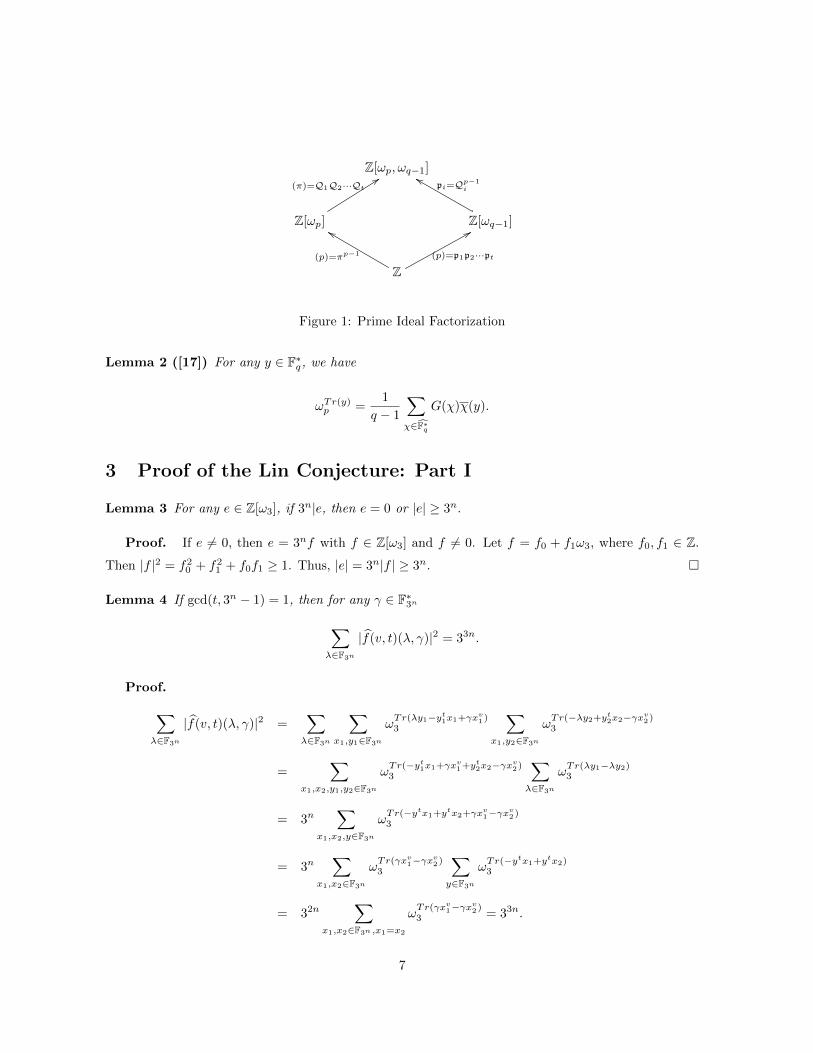
The factorization of prime ideals in algebraic integer rings is an interesting issue. (p) is a prime ideal
in Z. Let π = ωp − 1. It is known that (π) is a prime ideal in Z[ωp]. Moreover, (p) = (π)p−1 in Z[ωp],
and (π) = Q1Q2 · · · Qt in Z[ωp, ωq−1], where Qi are prime ideals in Z[ωp, ωq−1], and t = φ(pn − 1)/n.
Hence, (p) = (Q1Q2 · · · Qt)p−1 in Z[ωp, ωq−1]. On the other hand, (p) = p1p2 · · · pt in Z[ωq−1]. For each
pi, it is the (p− 1)-th power of a prime ideal in Z[ωp, ωq−1]. Without loss of generality, we may assume
that pi = Qp−1i . For the relationship among (p), pi, and Qi, the reader is referred to Figure 1.
For each Qi, we have Z[ωp, ωq−1]/Qi ∼= Fq because [Z[ωp, ωq−1]/Qi : Z/(p)] = n. Henceforth, we fix
one prime ideal Qi, and denote it by Q for simplicity. There is one special multiplicative character χ
on Fq satisfying
χ(x)(mod Q) = x.
This character is called the Teichmuller character. For simplicity, henceforth we denote it by χp. The
Teichmuller character has been used to investigate the dual of certain bent functions [15].
For any 0 ≤ k < q − 1, let k = k0 + k1p + · · · + kn−1pn−1 be the p-adic representation of k, where
0 ≤ ki < p for i = 0, 1, . . . , n − 1. Let wt(k) = k0 + k1 + · · · + kn−1, and σ(k) = k0!k1! · · · kn−1!.
Moreover, for any j, we use wt(j) and σ(j) to denote wt(j) and σ(j) respectively, where 0 ≤ j < q − 1
and j ≡ j (mod q − 1).
Theorem 1 (Stickelberger’s Theorem, [20]) For any 0 < k < q − 1, we have
G(χ−kp ) ≡ −πwt(k)
σ(k)(mod πwt(k)+p−1).
Let e = bwt(k)/(p− 1)c, where b·c is the floor function. Then pe‖G(χ−kp ) for any 0 < k < q − 1 by
Stickelberger’s theorem. The following lemma is extremely powerful, which will be used later.
6
Z[ωp, ωq−1]
Z[ωp]
(π)=Q1Q2···Qt99
Z[ωq−1]
pi=Qp−1i
ff
Z(p)=πp−1
ff
(p)=p1p2···pt
88
Figure 1: Prime Ideal Factorization
Lemma 2 ([17]) For any y ∈ F∗q , we have
ωTr(y)p =
1
q − 1
∑χ∈F∗q
G(χ)χ(y).
3 Proof of the Lin Conjecture: Part I
Lemma 3 For any e ∈ Z[ω3], if 3n|e, then e = 0 or |e| ≥ 3n.
Proof. If e 6= 0, then e = 3nf with f ∈ Z[ω3] and f 6= 0. Let f = f0 + f1ω3, where f0, f1 ∈ Z.
Then |f |2 = f20 + f2
1 + f0f1 ≥ 1. Thus, |e| = 3n|f | ≥ 3n. �
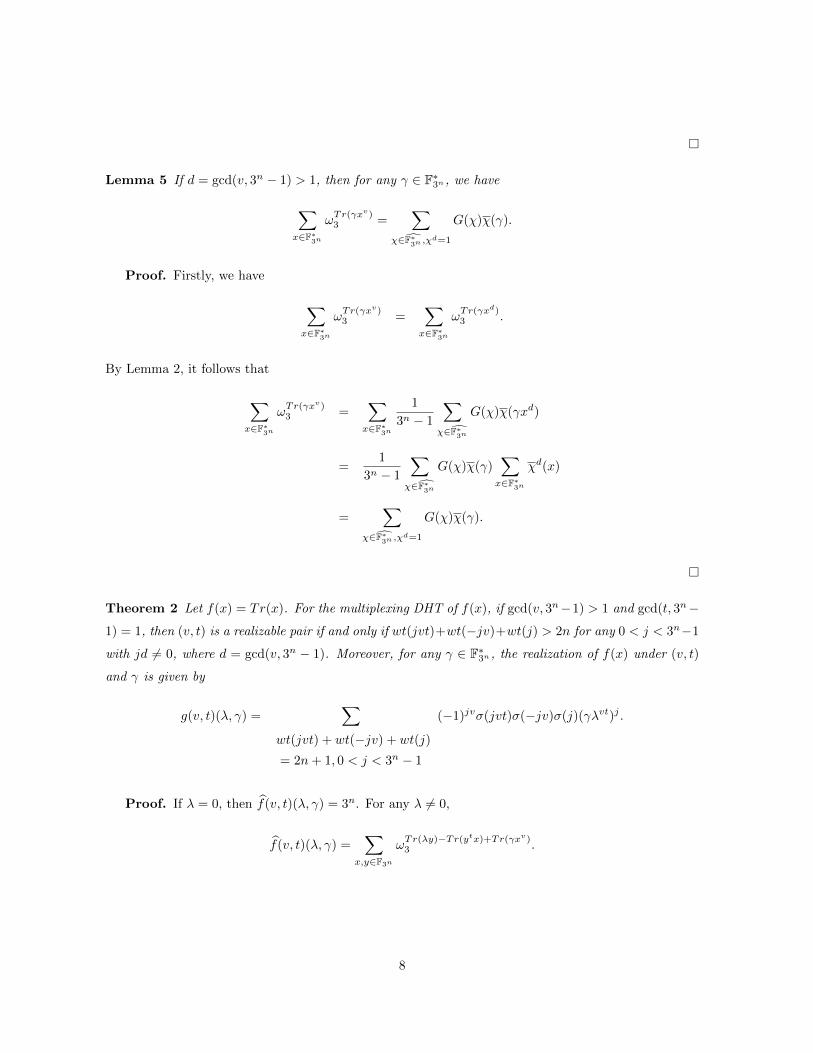
Lemma 4 If gcd(t, 3n − 1) = 1, then for any γ ∈ F∗3n∑λ∈F3n
|f(v, t)(λ, γ)|2 = 33n.
Proof.∑λ∈F3n
|f(v, t)(λ, γ)|2 =∑λ∈F3n
∑x1,y1∈F3n
ωTr(λy1−yt1x1+γxv1)3
∑x1,y2∈F3n
ωTr(−λy2+yt2x2−γxv2)3
=∑
x1,x2,y1,y2∈F3n
ωTr(−yt1x1+γxv1+yt2x2−γxv2)3
∑λ∈F3n
ωTr(λy1−λy2)3
= 3n∑
x1,x2,y∈F3n
ωTr(−ytx1+ytx2+γxv1−γx
v2)
3
= 3n∑
x1,x2∈F3n
ωTr(γxv1−γx
v2)
3
∑y∈F3n
ωTr(−ytx1+ytx2)3
= 32n∑
x1,x2∈F3n ,x1=x2
ωTr(γxv1−γx
v2)
3 = 33n.
7
�
Lemma 5 If d = gcd(v, 3n − 1) > 1, then for any γ ∈ F∗3n , we have
∑x∈F∗
3n
ωTr(γxv)3 =
∑χ∈F∗
3n,χd=1
G(χ)χ(γ).
Proof. Firstly, we have
∑x∈F∗
3n
ωTr(γxv)3 =
∑x∈F∗
3n
ωTr(γxd)3 .
By Lemma 2, it follows that
∑x∈F∗
3n
ωTr(γxv)3 =
∑x∈F∗
3n
1
3n − 1
∑χ∈F∗
3n
G(χ)χ(γxd)
=1
3n − 1
∑χ∈F∗
3n
G(χ)χ(γ)∑x∈F∗
3n
χd(x)
=∑
χ∈F∗3n,χd=1
G(χ)χ(γ).
�
Theorem 2 Let f(x) = Tr(x). For the multiplexing DHT of f(x), if gcd(v, 3n−1) > 1 and gcd(t, 3n−
1) = 1, then (v, t) is a realizable pair if and only if wt(jvt)+wt(−jv)+wt(j) > 2n for any 0 < j < 3n−1
with jd 6= 0, where d = gcd(v, 3n − 1). Moreover, for any γ ∈ F∗3n , the realization of f(x) under (v, t)
and γ is given by
g(v, t)(λ, γ) =∑
wt(jvt) + wt(−jv) + wt(j)
= 2n+ 1, 0 < j < 3n − 1
(−1)jvσ(jvt)σ(−jv)σ(j)(γλvt)j .
Proof. If λ = 0, then f(v, t)(λ, γ) = 3n. For any λ 6= 0,
f(v, t)(λ, γ) =∑
x,y∈F3n
ωTr(λy)−Tr(ytx)+Tr(γxv)3 .
8
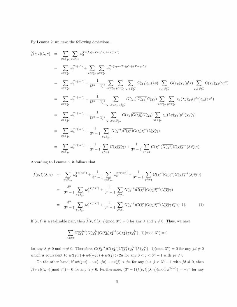
By Lemma 2, we have the following deviations.
f(v, t)(λ, γ) =∑x∈F∗
3n
∑y∈F3n
ωTr(λy)−Tr(ytx)+Tr(γxv)3
=∑x∈F∗
3n
ωTr(xv)3 +
∑x∈F∗
3n
∑y∈F∗
3n
ωTr(λy)−Tr(ytx)+Tr(γxv)3
=∑x∈F∗
3n
ωTr(γxv)3 +
1
(3n − 1)3
∑x∈F∗
3n
∑y∈F∗
3n
∑χ1∈F∗3n
G(χ1)χ1(λy)∑
χ2∈F∗3n
G(χ2)χ2(ytx)∑
χ3∈F∗3n
G(χ3)χ3(γxv)
=∑x∈F∗
3n
ωTr(γxv)3 +
1
(3n − 1)3
∑χ1,χ2,χ3∈F∗3n
G(χ1)G(χ2)G(χ3)∑x∈F∗
3n
∑y∈F∗
3n
χ1(λy)χ2(ytx)χ3(γxv)
=∑x∈F∗
3n
ωTr(γxv)3 +
1
(3n − 1)2
∑χ1,χ3∈F∗3n
G(χ1)G(χv3)G(χ3)∑y∈F∗
3n
χ1(λy)χ3(yvt)χ3(γ)
=∑x∈F∗
3n
ωTr(γxv)3 +
1
3n − 1
∑χ∈F∗
3n
G(χvt)G(χv)G(χ)χvt(λ)χ(γ)
=∑x∈F∗
3n
ωTr(γxv)3 +
1
3n − 1
∑χd=1
G(χ)χ(γ) +1
3n − 1
∑χd 6=1
G(χvt)G(χv)G(χ)χvt(λ)χ(γ).
According to Lemma 5, it follows that
f(v, t)(λ, γ) =∑x∈F∗
3n
ωTr(γxv)3 +
1
3n − 1
∑x∈F∗
3n
ωTr(γxv)3 +
1
3n − 1
∑χd 6=1
G(χvt)G(χv)G(χ)χvt(λ)χ(γ)
=3n
3n − 1
∑x∈F∗
3n
ωTr(γxv)3 +
1
3n − 1
∑χd 6=1
G(χvt)G(χv)G(χ)χvt(λ)χ(γ)
=3n
3n − 1
∑x∈F∗
3n
ωTr(γxv)3 +
1
3n − 1
∑χd 6=1
G(χvt)G(χv)G(χ)χvt(λ)χ(γ)χv(−1). (1)
If (v, t) is a realizable pair, then f(v, t)(λ, γ)(mod 3n) = 0 for any λ and γ 6= 0. Thus, we have
∑jd6=0
G(χjvtp )G(χjvp )G(χjp)χjvtp (λ)χjp(γ)χjvp (−1)(mod 3n) = 0
for any λ 6= 0 and γ 6= 0. Therefore, G(χjvtp )G(χjvp )G(χjp)χjvtp (λ)χjvp (−1)(mod 3n) = 0 for any jd 6= 0
which is equivalent to wt(jvt) + wt(−jv) + wt(j) > 2n for any 0 < j < 3n − 1 with jd 6= 0.
On the other hand, if wt(jvt) + wt(−jv) + wt(j) > 2n for any 0 < j < 3n − 1 with jd 6= 0, then
f(v, t)(λ, γ)(mod 3n) = 0 for any λ 6= 0. Furthermore, (3n − 1)f(v, t)(λ, γ)(mod π2n+1) = −3n for any
9
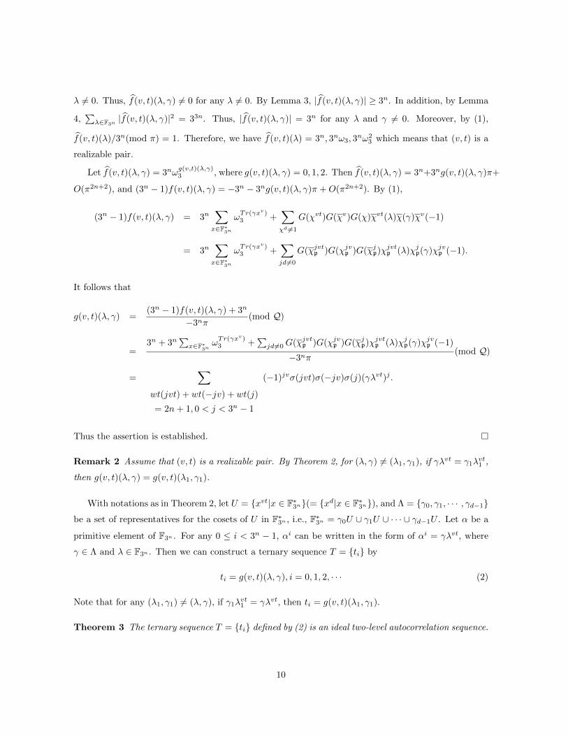
λ 6= 0. Thus, f(v, t)(λ, γ) 6= 0 for any λ 6= 0. By Lemma 3, |f(v, t)(λ, γ)| ≥ 3n. In addition, by Lemma
4,∑λ∈F3n
|f(v, t)(λ, γ)|2 = 33n. Thus, |f(v, t)(λ, γ)| = 3n for any λ and γ 6= 0. Moreover, by (1),
f(v, t)(λ)/3n(mod π) = 1. Therefore, we have f(v, t)(λ) = 3n, 3nω3, 3nω2
3 which means that (v, t) is a
realizable pair.
Let f(v, t)(λ, γ) = 3nωg(v,t)(λ,γ)3 , where g(v, t)(λ, γ) = 0, 1, 2. Then f(v, t)(λ, γ) = 3n+3ng(v, t)(λ, γ)π+
O(π2n+2), and (3n − 1)f(v, t)(λ, γ) = −3n − 3ng(v, t)(λ, γ)π +O(π2n+2). By (1),
(3n − 1)f(v, t)(λ, γ) = 3n∑x∈F∗
3n
ωTr(γxv)3 +
∑χd 6=1
G(χvt)G(χv)G(χ)χvt(λ)χ(γ)χv(−1)
= 3n∑x∈F∗
3n
ωTr(γxv)3 +
∑jd6=0
G(χjvtp )G(χjvp )G(χjp)χjvtp (λ)χjp(γ)χjvp (−1).
It follows that
g(v, t)(λ, γ) =(3n − 1)f(v, t)(λ, γ) + 3n
−3nπ(mod Q)
=3n + 3n
∑x∈F∗
3nωTr(γxv)3 +
∑jd6=0G(χjvtp )G(χjvp )G(χjp)χjvtp (λ)χjp(γ)χjvp (−1)
−3nπ(mod Q)
=∑
wt(jvt) + wt(−jv) + wt(j)
= 2n+ 1, 0 < j < 3n − 1
(−1)jvσ(jvt)σ(−jv)σ(j)(γλvt)j .
Thus the assertion is established. �
Remark 2 Assume that (v, t) is a realizable pair. By Theorem 2, for (λ, γ) 6= (λ1, γ1), if γλvt = γ1λvt1 ,
then g(v, t)(λ, γ) = g(v, t)(λ1, γ1).
With notations as in Theorem 2, let U = {xvt|x ∈ F∗3n}(= {xd|x ∈ F∗3n}), and Λ = {γ0, γ1, · · · , γd−1}
be a set of representatives for the cosets of U in F∗3n , i.e., F∗3n = γ0U ∪ γ1U ∪ · · · ∪ γd−1U . Let α be a
primitive element of F3n . For any 0 ≤ i < 3n − 1, αi can be written in the form of αi = γλvt, where
γ ∈ Λ and λ ∈ F3n . Then we can construct a ternary sequence T = {ti} by
ti = g(v, t)(λ, γ), i = 0, 1, 2, · · · (2)
Note that for any (λ1, γ1) 6= (λ, γ), if γ1λvt1 = γλvt, then ti = g(v, t)(λ1, γ1).
Theorem 3 The ternary sequence T = {ti} defined by (2) is an ideal two-level autocorrelation sequence.
10
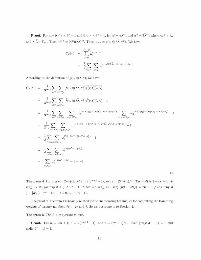
Proof. For any 0 ≤ i < 3n − 1 and 0 < τ < 3n − 1, let αi = γλvt, and ατ = γλvt, where γ, γ ∈ Λ,
and λ, λ ∈ F3n . Then αi+τ = (γγ)(λλ)vt. Thus, ti+τ = g(v, t)(λλ, γγ). We have
CT (τ) =
3n−2∑i=0
ωti+τ−ti3
=1
d
∑γ∈Λ
∑λ∈F∗
3n
ωg(v,t)(λλ,γγ)−g(v,t)(λ,γ)3 .
According to the definition of g(v, t)(λ, γ), we have
CS(τ) =1
32nd
∑γ∈Λ
∑λ∈F∗
3n
f(v, t)(λλ, γγ)f(v, t)(λ, γ)
=1
32nd
∑γ∈Λ
∑λ∈F3n
f(v, t)(λλ, γγ)f(v, t)(λ, γ)− 1
=1
32nd
∑γ∈Λ
∑λ∈F3n
∑x1,y1∈F3n
ωTr(λλy1)−Tr(yt1x1)+Tr(γγxv1)3
∑x2,y2∈F3n
ω−Tr(λy2)+Tr(yt2x2)−Tr(γxv2)3 − 1
=1
3nd
∑γ∈Λ
∑x1,x2,y∈F3n
ω−Tr(ytx1)+Tr(γγxv1)+Tr(λtytx2)−Tr(γxv2)3 − 1
=1
d
∑γ∈Λ
∑x2∈F3n
ωTr(γγλvtxv2)−Tr(γxv2)3 − 1
=1
d
∑γ∈Λ
∑x2∈F3n
ωTr((ατ−1)γxv2)3 − 1
=∑x∈F3n
ωTr((ατ−1)x)3 − 1 = −1.
�
Theorem 4 For any n = 2m+ 1, let v = 2(3m+1− 1), and t = (3n + 1)/4. Then wt(jvt) +wt(−jv) +
wt(j) > 2n for any 0 < j < 3n − 1. Moreover, wt(jvt) + wt(−jv) + wt(j) = 2n + 1 if and only if
j ∈ {3i, (2 · 3m + 1)3i | i = 0, 1, · · · , n− 1}.
The proof of Theorem 4 is heavily related to the enumerating techniques for computing the Hamming
weights of ternary numbers jvt,−jv and j. So we postpone it to Section 4.
Theorem 5 The Lin conjecture is true.
Proof. Let n = 2m + 1, v = 2(3m+1 − 1), and t = (3n + 1)/4. Then gcd(v, 3n − 1) = 2 and
gcd(t, 3n − 1) = 1.
11
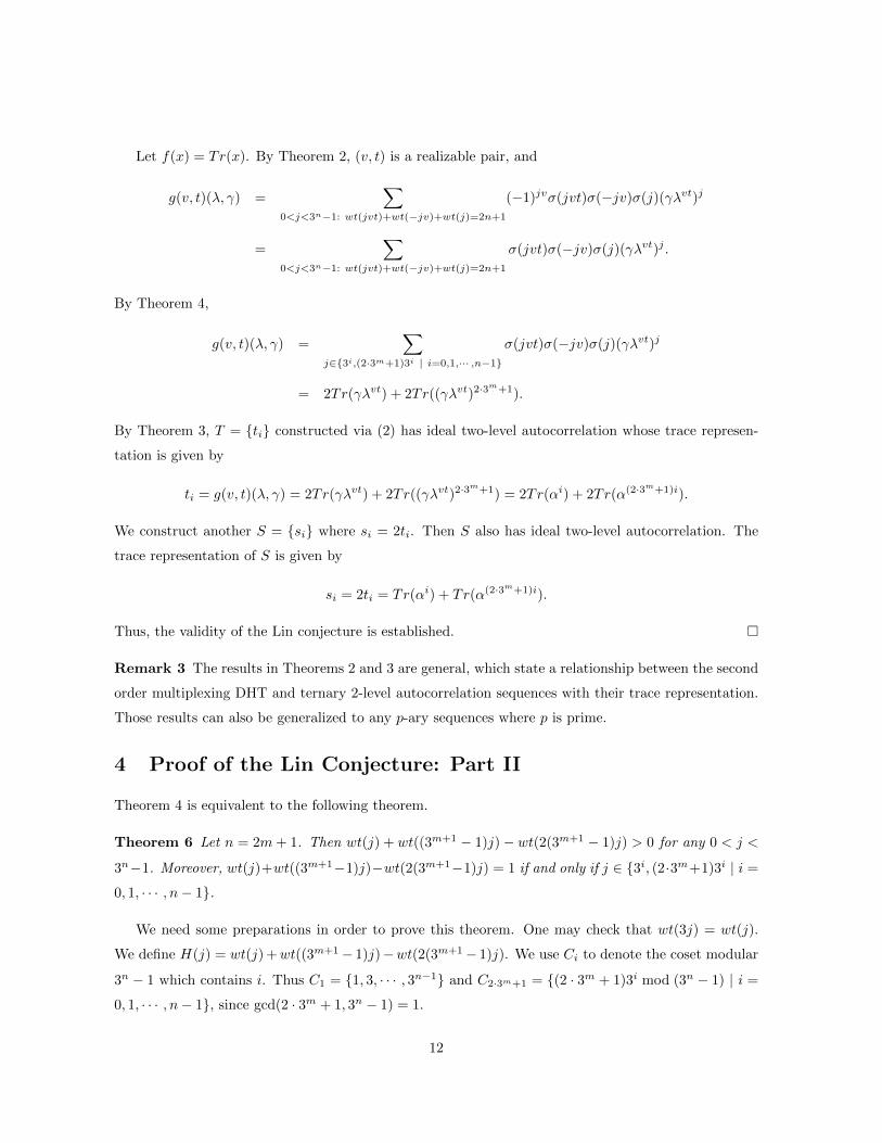
Let f(x) = Tr(x). By Theorem 2, (v, t) is a realizable pair, and
g(v, t)(λ, γ) =∑
0<j<3n−1: wt(jvt)+wt(−jv)+wt(j)=2n+1
(−1)jvσ(jvt)σ(−jv)σ(j)(γλvt)j
=∑
0<j<3n−1: wt(jvt)+wt(−jv)+wt(j)=2n+1
σ(jvt)σ(−jv)σ(j)(γλvt)j .
By Theorem 4,
g(v, t)(λ, γ) =∑
j∈{3i,(2·3m+1)3i | i=0,1,··· ,n−1}
σ(jvt)σ(−jv)σ(j)(γλvt)j
= 2Tr(γλvt) + 2Tr((γλvt)2·3m+1).
By Theorem 3, T = {ti} constructed via (2) has ideal two-level autocorrelation whose trace represen-
tation is given by
ti = g(v, t)(λ, γ) = 2Tr(γλvt) + 2Tr((γλvt)2·3m+1) = 2Tr(αi) + 2Tr(α(2·3m+1)i).
We construct another S = {si} where si = 2ti. Then S also has ideal two-level autocorrelation. The
trace representation of S is given by
si = 2ti = Tr(αi) + Tr(α(2·3m+1)i).
Thus, the validity of the Lin conjecture is established. �
Remark 3 The results in Theorems 2 and 3 are general, which state a relationship between the second
order multiplexing DHT and ternary 2-level autocorrelation sequences with their trace representation.
Those results can also be generalized to any p-ary sequences where p is prime.
4 Proof of the Lin Conjecture: Part II
Theorem 4 is equivalent to the following theorem.
Theorem 6 Let n = 2m+ 1. Then wt(j) + wt((3m+1 − 1)j)− wt(2(3m+1 − 1)j) > 0 for any 0 < j <
3n−1. Moreover, wt(j)+wt((3m+1−1)j)−wt(2(3m+1−1)j) = 1 if and only if j ∈ {3i, (2·3m+1)3i | i =
0, 1, · · · , n− 1}.
We need some preparations in order to prove this theorem. One may check that wt(3j) = wt(j).
We define H(j) = wt(j) +wt((3m+1− 1)j)−wt(2(3m+1− 1)j). We use Ci to denote the coset modular
3n − 1 which contains i. Thus C1 = {1, 3, · · · , 3n−1} and C2·3m+1 = {(2 · 3m + 1)3i mod (3n − 1) | i =
0, 1, · · · , n− 1}, since gcd(2 · 3m + 1, 3n − 1) = 1.
12
For any a > 0, we denote the residue of a modulo 3n− 1 by a, i.e., a ≡ a (mod 3n− 1) and 0 ≤ a <
3n − 1. If a =∑2mi=0 ai3
i with ai ∈ {0, 1, 2}, then we write it as a = a2ma2m−1 · · · a1a0 for simplicity,
i.e., a2ma2m−1 · · · a1a0 is the ternary representation of a. However, if it is clear that 0 < a < 3n − 1,
sometimes, we also directly write a instead of a for simplicity. For any 0 ≤ i ≤ 2m, using the shift
operation, we define an equivalent relationship on: (a2ma2m−1 · · · a1a0) ∼ (aiai−1 · · · a0a2m · · · ai+1).
The shift operation does not change the value of H(j), i.e., we have
H(3ij) = H(j), i = 0, 1, · · · , n− 1, 0 < j < 3n − 1. (3)
Thus, for the assertion of Theorem 6, we only need to show that for one j in its equivalent class.
We need two more notations. For any r ≥ 0, let
Rr0 = 11 · · · 11︸ ︷︷ ︸r
0 and Rr2 = 11 · · · 11︸ ︷︷ ︸r
2.
Then a ∼ bt−1bt−2 · · · b0, where bi = Rri0 or Rri2, i = 0, 1, · · · , t− 1, and t ≥ 1.
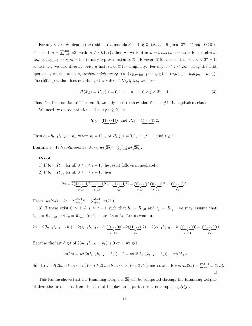
Lemma 6 With notations as above, wt(2a) =∑t−1i=0 wt(2bi).
Proof.
1) If bi = Rri0 for all 0 ≤ i ≤ t− 1, the result follows immediately.
2) If bi = Rri2 for all 0 ≤ i ≤ t− 1, then
2a = 2(11 · · · 1︸ ︷︷ ︸rt−1
2 11 · · · 1︸ ︷︷ ︸rt−2
2 · · · 11 · · · 1︸ ︷︷ ︸r0
2) = 00 · · · 0︸ ︷︷ ︸rt−1
2 00 · · · 0︸ ︷︷ ︸rt−2
2 · · · 00 · · · 0︸ ︷︷ ︸r0
2.
Hence, wt(2a) = 2t =∑t−1i=0 2 =
∑t−1i=0 wt(2bi).
3) If these exist 0 ≤ i 6= j ≤ t − 1 such that bi = Rri0 and bj = Rrj2, we may assume that
bt−1 = Rrt−10 and b0 = Rr02. In this case, 2a = 2a. Let us compute
2a = 2(bt−1bt−2 · · · b0) = 2(bt−1bt−2 · · · b1 00 · · · 00︸ ︷︷ ︸r0+1
)+2(11 · · · 1︸ ︷︷ ︸r0
2) = 2(bt−1bt−2 · · · b1 00 · · · 00︸ ︷︷ ︸r0+1
)+1 00 · · · 00︸ ︷︷ ︸r0
1.
Because the last digit of 2(bt−1bt−2 · · · b1) is 0 or 1, we get
wt(2a) = wt(2(bt−1bt−2 · · · b1)) + 2 = wt(2(bt−1bt−2 · · · b1)) + wt(2b0).
Similarly, wt(2(bt−1bt−2 · · · b1)) = wt(2(bt−1bt−2 · · · b2))+wt(2b1), and so on. Hence, wt(2a) =∑t−1i=0 wt(2bi).
�
This lemma shows that the Hamming weight of 2a can be computed through the Hamming weights
of their the runs of 1’s. Here the runs of 1’s play an important rule in computing H(j).
13
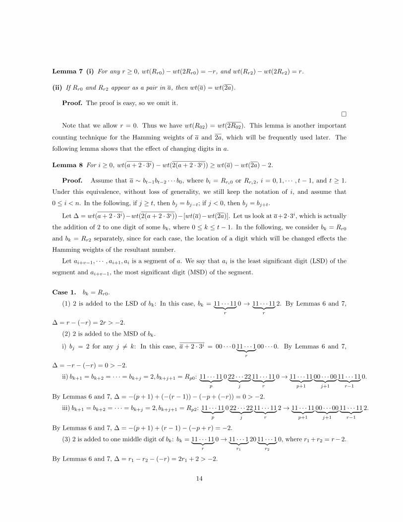
Lemma 7 (i) For any r ≥ 0, wt(Rr0)− wt(2Rr0) = −r, and wt(Rr2)− wt(2Rr2) = r.
(ii) If Rr0 and Rr2 appear as a pair in a, then wt(a) = wt(2a).
Proof. The proof is easy, so we omit it.
�
Note that we allow r = 0. Thus we have wt(R02) = wt(2R02). This lemma is another important
counting technique for the Hamming weights of a and 2a, which will be frequently used later. The
following lemma shows that the effect of changing digits in a.
Lemma 8 For i ≥ 0, wt(a+ 2 · 3i)− wt(2(a+ 2 · 3i)) ≥ wt(a)− wt(2a)− 2.
Proof. Assume that a ∼ bt−1bt−2 · · · b0, where bi = Rri0 or Rri2, i = 0, 1, · · · , t − 1, and t ≥ 1.
Under this equivalence, without loss of generality, we still keep the notation of i, and assume that
0 ≤ i < n. In the following, if j ≥ t, then bj = bj−t; if j < 0, then bj = bj+t.
Let ∆ = wt(a+ 2 · 3i)−wt(2(a+ 2 · 3i))− [wt(a)−wt(2a)]. Let us look at a+2 ·3i, which is actually
the addition of 2 to one digit of some bk, where 0 ≤ k ≤ t− 1. In the following, we consider bk = Rr0
and bk = Rr2 separately, since for each case, the location of a digit which will be changed effects the
Hamming weights of the resultant number.
Let ai+v−1, · · · , ai+1, ai is a segment of a. We say that ai is the least significant digit (LSD) of the
segment and ai+v−1, the most significant digit (MSD) of the segment.
Case 1. bk = Rr0.
(1) 2 is added to the LSD of bk: In this case, bk = 11 · · · 11︸ ︷︷ ︸r
0 → 11 · · · 11︸ ︷︷ ︸r
2. By Lemmas 6 and 7,
∆ = r − (−r) = 2r > −2.
(2) 2 is added to the MSD of bk.
i) bj = 2 for any j 6= k: In this case, a+ 2 · 3i = 00 · · · 0 11 · · · 1︸ ︷︷ ︸r
00 · · · 0. By Lemmas 6 and 7,
∆ = −r − (−r) = 0 > −2.
ii) bk+1 = bk+2 = · · · = bk+j = 2, bk+j+1 = Rp0: 11 · · · 11︸ ︷︷ ︸p
0 22 · · · 22︸ ︷︷ ︸j
11 · · · 11︸ ︷︷ ︸r
0→ 11 · · · 11︸ ︷︷ ︸p+1
00 · · · 00︸ ︷︷ ︸j+1
11 · · · 11︸ ︷︷ ︸r−1
0.
By Lemmas 6 and 7, ∆ = −(p+ 1) + (−(r − 1))− (−p+ (−r)) = 0 > −2.
iii) bk+1 = bk+2 = · · · = bk+j = 2, bk+j+1 = Rp2: 11 · · · 11︸ ︷︷ ︸p
0 22 · · · 22︸ ︷︷ ︸j
11 · · · 11︸ ︷︷ ︸r
2→ 11 · · · 11︸ ︷︷ ︸p+1
00 · · · 00︸ ︷︷ ︸j+1
11 · · · 11︸ ︷︷ ︸r−1
2.
By Lemmas 6 and 7, ∆ = −(p+ 1) + (r − 1)− (−p+ r) = −2.
(3) 2 is added to one middle digit of bk: bk = 11 · · · 11︸ ︷︷ ︸r
0→ 11 · · · 1︸ ︷︷ ︸r1
20 11 · · · 1︸ ︷︷ ︸r2
0, where r1 +r2 = r−2.
By Lemmas 6 and 7, ∆ = r1 − r2 − (−r) = 2r1 + 2 > −2.
14

Case 2. bk = Rr2.
(1) 2 is added to the LSD of bk.
i) r > 0 and bk−1 = Rt0: 11 · · · 11︸ ︷︷ ︸r
2 11 · · · 111︸ ︷︷ ︸t
0 → 11 · · · 11︸ ︷︷ ︸r−1
21 11 · · · 111︸ ︷︷ ︸t
0. By Lemmas 6 and 7,
∆ = (r − 1) + (−(t+ 1))− (r + (−t)) = −2.
ii) r > 0 and bk−1 = Rt2: 11 · · · 11︸ ︷︷ ︸r
2 11 · · · 111︸ ︷︷ ︸t
2 → 11 · · · 11︸ ︷︷ ︸r−1
21 11 · · · 111︸ ︷︷ ︸t
2. By Lemmas 6 and 7,
∆ = (r − 1) + (t+ 1)− (r + t) = 0.
iii) bk = bk+1 = · · · = bk+j = 2, bk+j+1 = Rp2, bk−1 = Rt0: 11 · · · 11︸ ︷︷ ︸p
22..2︸︷︷︸j+2
11 · · · 1︸ ︷︷ ︸t
0→ 11 · · · 11︸ ︷︷ ︸p−1
2 00..0︸︷︷︸j+1
11 · · · 1︸ ︷︷ ︸t+1
0.
By Lemmas 6 and 7, ∆ = (p− 1) + (−(t+ 1))− (p+ (−t)) = −2.
iv) bk = bk+1 = · · · = bk+j = 2, bk+j+1 = Rp2, bk−1 = Rt2: 11 · · · 11︸ ︷︷ ︸p
22..2︸︷︷︸j+2
11 · · · 1︸ ︷︷ ︸t
2→ 11 · · · 11︸ ︷︷ ︸p−1
2 00..0︸︷︷︸j+1
11 · · · 1︸ ︷︷ ︸t+1
2.
By Lemmas 6 and 7, ∆ = (p− 1) + (t+ 1)− (p+ t) = 0.
v) bk = bk+1 = · · · = bk+j = 2, bk+j+1 = Rp0, bk−1 = Rt0: 11 · · · 11︸ ︷︷ ︸p
0 22..2︸︷︷︸j+1
11 · · · 1︸ ︷︷ ︸t
0→ 11 · · · 11︸ ︷︷ ︸p+1
00..0︸︷︷︸j
11 · · · 1︸ ︷︷ ︸t+1
0.
By Lemmas 6 and 7, ∆ = −(p+ 1) + (−(t+ 1))− (−p− t) = −2.
vi) bk = bk+1 = · · · = bk+j = 2, bk+j+1 = Rp0, bk−1 = Rt2: 11 · · · 11︸ ︷︷ ︸p
0 22..2︸︷︷︸j+1
11 · · · 1︸ ︷︷ ︸t
2→ 11 · · · 11︸ ︷︷ ︸p+1
00..0︸︷︷︸j
11 · · · 1︸ ︷︷ ︸t+1
2.
By Lemmas 6 and 7, ∆ = −(p+ 1) + (t+ 1)− (−p+ t) = 0.
(2) 2 is added to the MSD of bk.
i) bj = 2 for any j 6= k: In this case, a+ 2 · 3i = 00 · · · 0 11 · · · 1︸ ︷︷ ︸r−2
20 · · · 0, where r ≥ 2, or
00 · · · 0100 · · · 0, where r = 1. Thus, ∆ = r − 2− r = −2 or ∆ = −1− 1 = −2.
ii) bk+1 = bk+2 = · · · = bk+j = 2, bk+j+1 = Rp0: 11 · · · 11︸ ︷︷ ︸p
0 22 · · · 2︸ ︷︷ ︸j
11 · · · 1︸ ︷︷ ︸r
2→ 11 · · · 11︸ ︷︷ ︸p+1
00..0︸︷︷︸j+1
11 · · · 1︸ ︷︷ ︸r−1
2.
By Lemmas 6 and 7, ∆ = −(p+ 1) + (r − 1)− (−p+ r) = −2.
iii) bk+1 = bk+2 = · · · = bk+j = 2, bk+j+1 = Rp2: 11 · · · 11︸ ︷︷ ︸p
22 · · · 2︸ ︷︷ ︸j+1
11 · · · 1︸ ︷︷ ︸r
2→ 11 · · · 11︸ ︷︷ ︸p−1
2 00..0︸︷︷︸j+2
11 · · · 1︸ ︷︷ ︸r−1
2.
By Lemmas 6 and 7, ∆ = (p− 1) + (r − 1)− (p+ r) = −2.
(3) 2 is added to the middle digit of bk: bk = 11 · · · 11︸ ︷︷ ︸r
2→ 11 · · · 1︸ ︷︷ ︸r1
20 11 · · · 1︸ ︷︷ ︸r2
2, where r1 + r2 = r−2.
By Lemmas 6 and 7, ∆ = r1 − r2 − r = −2.
�
Lemma 9 For any i, j > 0, we have
(3m+1 − 1)[j ± (3m+1 + 1)3i] ≡ (3m+1 − 1)j ± 2 · 3i (mod 3n − 1).
15
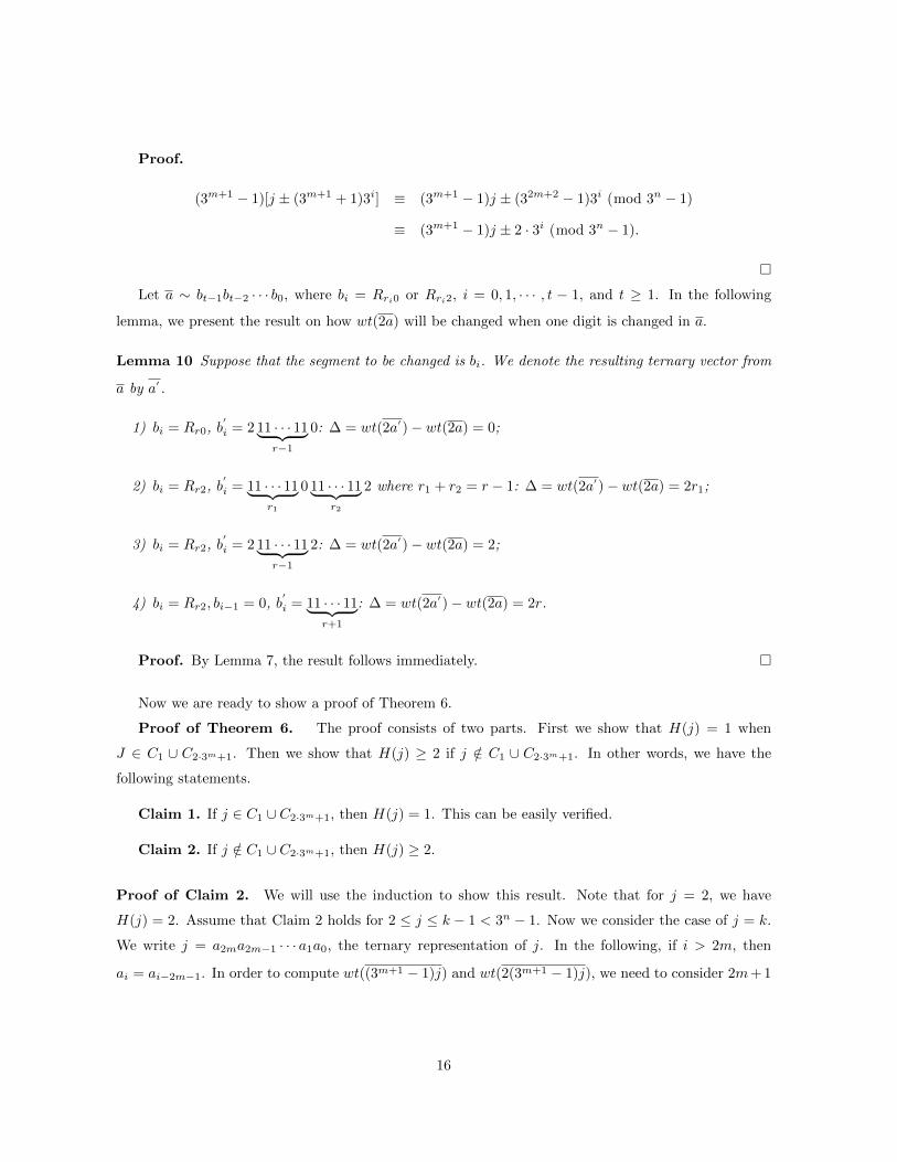
Proof.
(3m+1 − 1)[j ± (3m+1 + 1)3i] ≡ (3m+1 − 1)j ± (32m+2 − 1)3i (mod 3n − 1)
≡ (3m+1 − 1)j ± 2 · 3i (mod 3n − 1).
�
Let a ∼ bt−1bt−2 · · · b0, where bi = Rri0 or Rri2, i = 0, 1, · · · , t − 1, and t ≥ 1. In the following
lemma, we present the result on how wt(2a) will be changed when one digit is changed in a.
Lemma 10 Suppose that the segment to be changed is bi. We denote the resulting ternary vector from
a by a′ .
1) bi = Rr0, b′
i = 2 11 · · · 11︸ ︷︷ ︸r−1
0: ∆ = wt(2a′)− wt(2a) = 0;
2) bi = Rr2, b′
i = 11 · · · 11︸ ︷︷ ︸r1
0 11 · · · 11︸ ︷︷ ︸r2
2 where r1 + r2 = r − 1: ∆ = wt(2a′)− wt(2a) = 2r1;
3) bi = Rr2, b′
i = 2 11 · · · 11︸ ︷︷ ︸r−1
2: ∆ = wt(2a′)− wt(2a) = 2;
4) bi = Rr2, bi−1 = 0, b′
i = 11 · · · 11︸ ︷︷ ︸r+1
: ∆ = wt(2a′)− wt(2a) = 2r.
Proof. By Lemma 7, the result follows immediately. �
Now we are ready to show a proof of Theorem 6.
Proof of Theorem 6. The proof consists of two parts. First we show that H(j) = 1 when
J ∈ C1 ∪ C2·3m+1. Then we show that H(j) ≥ 2 if j /∈ C1 ∪ C2·3m+1. In other words, we have the
following statements.
Claim 1. If j ∈ C1 ∪ C2·3m+1, then H(j) = 1. This can be easily verified.
Claim 2. If j /∈ C1 ∪ C2·3m+1, then H(j) ≥ 2.
Proof of Claim 2. We will use the induction to show this result. Note that for j = 2, we have
H(j) = 2. Assume that Claim 2 holds for 2 ≤ j ≤ k − 1 < 3n − 1. Now we consider the case of j = k.
We write j = a2ma2m−1 · · · a1a0, the ternary representation of j. In the following, if i > 2m, then
ai = ai−2m−1. In order to compute wt((3m+1 − 1)j) and wt(2(3m+1 − 1)j), we need to consider 2m+ 1
16
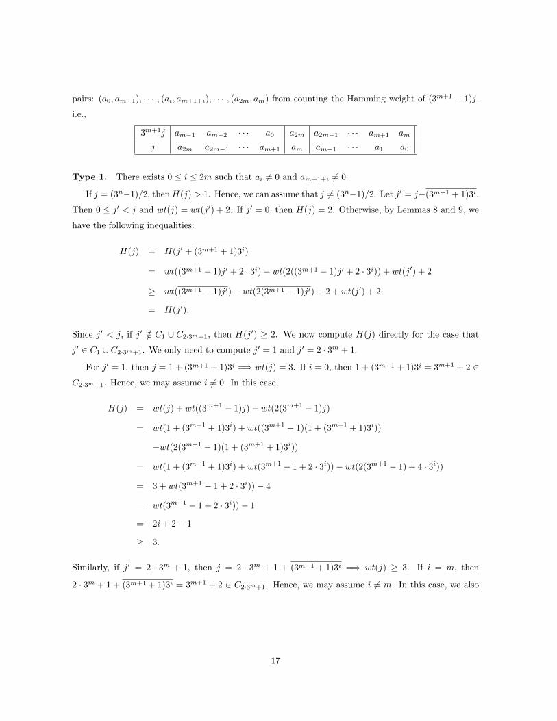
pairs: (a0, am+1), · · · , (ai, am+1+i), · · · , (a2m, am) from counting the Hamming weight of (3m+1 − 1)j,
i.e.,
3m+1j am−1 am−2 · · · a0 a2m a2m−1 · · · am+1 am
j a2m a2m−1 · · · am+1 am am−1 · · · a1 a0
Type 1. There exists 0 ≤ i ≤ 2m such that ai 6= 0 and am+1+i 6= 0.
If j = (3n−1)/2, thenH(j) > 1. Hence, we can assume that j 6= (3n−1)/2. Let j′ = j−(3m+1 + 1)3i.
Then 0 ≤ j′ < j and wt(j) = wt(j′) + 2. If j′ = 0, then H(j) = 2. Otherwise, by Lemmas 8 and 9, we
have the following inequalities:
H(j) = H(j′ + (3m+1 + 1)3i)
= wt((3m+1 − 1)j′ + 2 · 3i)− wt(2((3m+1 − 1)j′ + 2 · 3i)) + wt(j′) + 2
≥ wt((3m+1 − 1)j′)− wt(2(3m+1 − 1)j′)− 2 + wt(j′) + 2
= H(j′).
Since j′ < j, if j′ /∈ C1 ∪ C2·3m+1, then H(j′) ≥ 2. We now compute H(j) directly for the case that
j′ ∈ C1 ∪ C2·3m+1. We only need to compute j′ = 1 and j′ = 2 · 3m + 1.
For j′ = 1, then j = 1 + (3m+1 + 1)3i =⇒ wt(j) = 3. If i = 0, then 1 + (3m+1 + 1)3i = 3m+1 + 2 ∈
C2·3m+1. Hence, we may assume i 6= 0. In this case,
H(j) = wt(j) + wt((3m+1 − 1)j)− wt(2(3m+1 − 1)j)
= wt(1 + (3m+1 + 1)3i) + wt((3m+1 − 1)(1 + (3m+1 + 1)3i))
−wt(2(3m+1 − 1)(1 + (3m+1 + 1)3i))
= wt(1 + (3m+1 + 1)3i) + wt(3m+1 − 1 + 2 · 3i))− wt(2(3m+1 − 1) + 4 · 3i))
= 3 + wt(3m+1 − 1 + 2 · 3i))− 4
= wt(3m+1 − 1 + 2 · 3i))− 1
= 2i+ 2− 1
≥ 3.
Similarly, if j′ = 2 · 3m + 1, then j = 2 · 3m + 1 + (3m+1 + 1)3i =⇒ wt(j) ≥ 3. If i = m, then
2 · 3m + 1 + (3m+1 + 1)3i = 3m+1 + 2 ∈ C2·3m+1. Hence, we may assume i 6= m. In this case, we also
17
have
H(j) = wt(j) + wt((3m+1 − 1)j)− wt(2(3m+1 − 1)j)
= wt(2 · 3m + 1 + (3m+1 + 1)3i) + wt((3m+1 − 1)(2 · 3m + 1 + (3m+1 + 1)3i))
−wt(2(3m+1 − 1)(2 · 3m + 1 + (3m+1 + 1)3i))
= wt(2 · 3m + 1 + (3m+1 + 1)3i) + wt((3m+1 − 1)(2 · 3m + 1) + 2 · 3i)
−wt(2(3m+1 − 1)(2 · 3m + 1) + 4 · 3i)
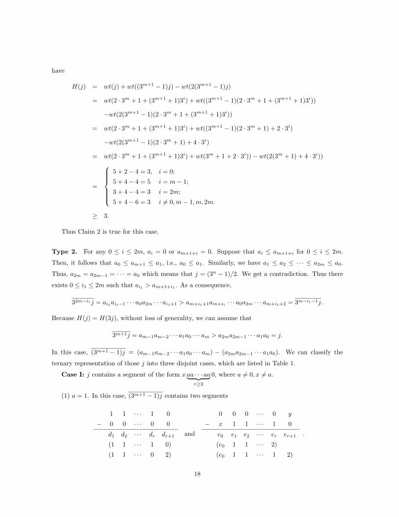
= wt(2 · 3m + 1 + (3m+1 + 1)3i) + wt(3m + 1 + 2 · 3i))− wt(2(3m + 1) + 4 · 3i))
=
5 + 2− 4 = 3, i = 0;
5 + 4− 4 = 5 i = m− 1;
3 + 4− 4 = 3 i = 2m;
5 + 4− 6 = 3 i 6= 0,m− 1,m, 2m.
≥ 3.
Thus Claim 2 is true for this case.
Type 2. For any 0 ≤ i ≤ 2m, ai = 0 or am+1+i = 0. Suppose that ai ≤ am+1+i for 0 ≤ i ≤ 2m.
Then, it follows that a0 ≤ am+1 ≤ a1, i.e., a0 ≤ a1. Similarly, we have a1 ≤ a2 ≤ · · · ≤ a2m ≤ a0.
Thus, a2m = a2m−1 = · · · = a0 which means that j = (3n − 1)/2. We get a contradiction. Thus there
exists 0 ≤ i1 ≤ 2m such that ai1 > am+1+i1 . As a consequence,
32m−i1j = ai1ai1−1 · · · a0a2m · · · ai1+1 > am+i1+1am+i1 · · · a0a2m · · · am+i1+2 = 3m−i1−1j.
Because H(j) = H(3j), without loss of generality, we can assume that
3m+1j = am−1am−2 · · · a1a0 · · · am > a2ma2m−1 · · · a1a0 = j.
In this case, (3m+1 − 1)j = (am−1am−2 · · · a1a0 · · · am) − (a2ma2m−1 · · · a1a0). We can classify the
ternary representation of those j into three disjoint cases, which are listed in Table 1.
Case I: j contains a segment of the form x aa · · · aa︸ ︷︷ ︸r≥2
0, where a 6= 0, x 6= a.
(1) a = 1. In this case, (3m+1 − 1)j contains two segments
1 1 · · · 1 0
− 0 0 · · · 0 0
d1 d2 · · · dr dr+1
(1 1 · · · 1 0)
(1 1 · · · 0 2)
and
0 0 0 · · · 0 y
− x 1 1 · · · 1 0
e0 e1 e2 · · · er er+1
(e0 1 1 · · · 2)
(e0 1 1 · · · 1 2)
.
18

Table 1: Three Disjoint Cases of Patterns in the Ternary Representation of j with ai = 0 or ai+m−1 = 0
for all 0 ≤ i ≤ 2m
Patterns
Case I x aa · · · aa︸ ︷︷ ︸r≥2
0: a 6= 0, x 6= a
Case II x aa · · · aa︸ ︷︷ ︸r≥1
b0: a 6= 0, b 6= 0, a 6= b, x 6= a
Case III 0a0: a 6= 0
In other words, d1 = d2 = · · · = dr−1 = 1, dr = 1, dr+1 = 0, or dr = 0, dr+1 = 2; e1 = e2 = · · · = er−1 =
1, er = 2, or er = 1, er+1 = 2. Because x 6= 1, e0 6= 1. We change the segment of j from 11 · · · 11︸ ︷︷ ︸r≥2
0
to 01 · · · 11︸ ︷︷ ︸r≥2
0, and denote the new integer by j′. Then d
′
1 = 0, e′
1 = 2, and other di, ei stay the same.
Therefore, wt((3m+1− 1)j′) = wt((3m+1− 1)j). By Lemma 10, wt(2(3m+1− 1)j
′) ≥ wt(2(3m+1− 1)j).
Moreover, wt(j) = wt(j′) + 1. Therefore, H(j) ≥ H(j
′) + 1 ≥ 2.
(2) a = 2. In this case, (3m+1 − 1)j contains two segments
2 2 · · · 2 0
− 0 0 · · · 0 0
d1 d2 · · · dr dr+1
(2 2 · · · 1 2)
(2 2 · · · 2 0)
and
0 0 0 · · · 0 y
− x 2 2 · · · 2 0
e0 e1 e2 · · · er er+1
(e0 0 0 · · · 0 2)
(e0 0 0 · · · 1 y)
.
In other words, d1 = d2 = · · · = dr−1 = 2, dr = 1, dr+1 = 2, or dr = 2, dr+1 = 0; e0 = 1 or 2,
e1 = e2 = · · · = er−1 = 0, er = 0, er+1 = 2, or er = 1, er+1 = y or y − 1. We change the segment
from 0 22 · · · 22︸ ︷︷ ︸r≥2
0 to 0 22 · · · 21︸ ︷︷ ︸r≥2
0, and denote the new integer by j′. Then d
′
r = dr − 1, e′
r = er + 1,
and other di, ei stay the same. Therefore, wt((3m+1 − 1)j′) = wt((3m+1 − 1)j). By Lemma 10,
wt(2(3m+1−1)j′) ≥ wt(2(3m+1−1)j). Moreover, wt(j) = wt(j
′)+1. Therefore, H(j) ≥ H(j
′)+1 ≥ 2.
Case II: j contains a segment of the form x aa · · · aa︸ ︷︷ ︸r≥1
b0, where a 6= 0, b 6= 0, a 6= b, x 6= a.
19
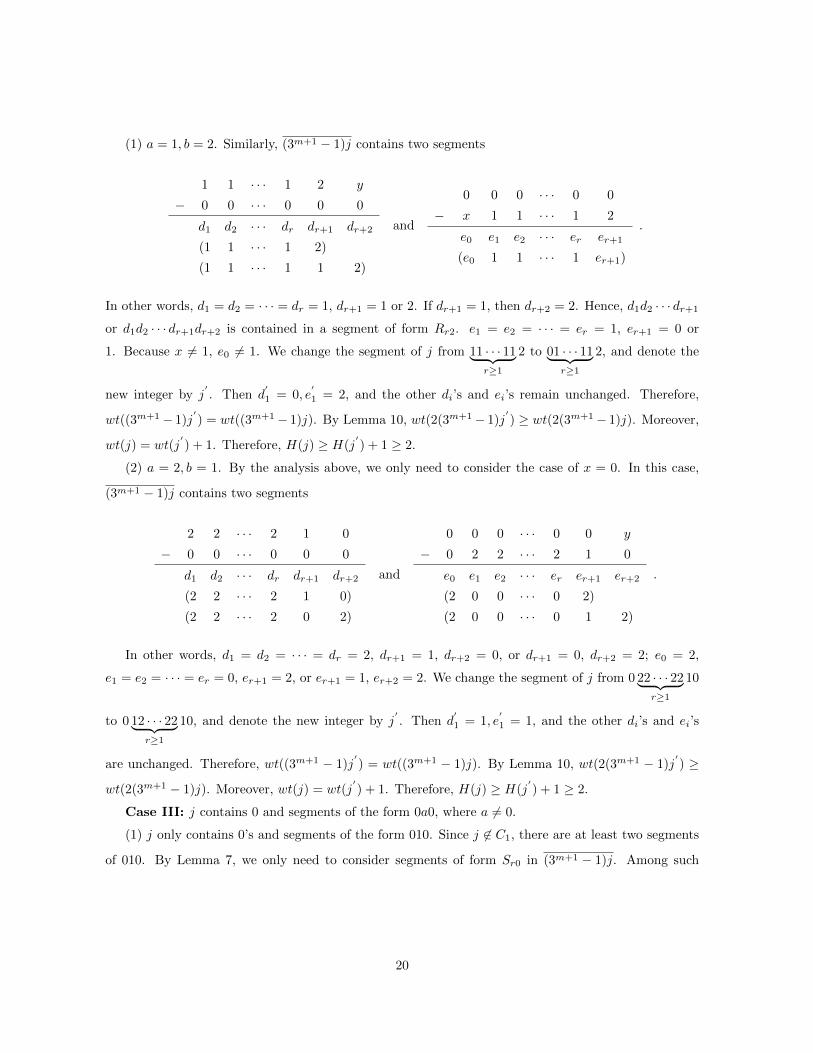
(1) a = 1, b = 2. Similarly, (3m+1 − 1)j contains two segments
1 1 · · · 1 2 y
− 0 0 · · · 0 0 0
d1 d2 · · · dr dr+1 dr+2
(1 1 · · · 1 2)
(1 1 · · · 1 1 2)
and
0 0 0 · · · 0 0
− x 1 1 · · · 1 2
e0 e1 e2 · · · er er+1
(e0 1 1 · · · 1 er+1)
.
In other words, d1 = d2 = · · · = dr = 1, dr+1 = 1 or 2. If dr+1 = 1, then dr+2 = 2. Hence, d1d2 · · · dr+1
or d1d2 · · · dr+1dr+2 is contained in a segment of form Rr2. e1 = e2 = · · · = er = 1, er+1 = 0 or
1. Because x 6= 1, e0 6= 1. We change the segment of j from 11 · · · 11︸ ︷︷ ︸r≥1
2 to 01 · · · 11︸ ︷︷ ︸r≥1
2, and denote the
new integer by j′. Then d
′
1 = 0, e′
1 = 2, and the other di’s and ei’s remain unchanged. Therefore,
wt((3m+1− 1)j′) = wt((3m+1− 1)j). By Lemma 10, wt(2(3m+1− 1)j
′) ≥ wt(2(3m+1− 1)j). Moreover,
wt(j) = wt(j′) + 1. Therefore, H(j) ≥ H(j
′) + 1 ≥ 2.
(2) a = 2, b = 1. By the analysis above, we only need to consider the case of x = 0. In this case,
(3m+1 − 1)j contains two segments
2 2 · · · 2 1 0
− 0 0 · · · 0 0 0
d1 d2 · · · dr dr+1 dr+2
(2 2 · · · 2 1 0)
(2 2 · · · 2 0 2)
and
0 0 0 · · · 0 0 y
− 0 2 2 · · · 2 1 0
e0 e1 e2 · · · er er+1 er+2
(2 0 0 · · · 0 2)
(2 0 0 · · · 0 1 2)
.
In other words, d1 = d2 = · · · = dr = 2, dr+1 = 1, dr+2 = 0, or dr+1 = 0, dr+2 = 2; e0 = 2,
e1 = e2 = · · · = er = 0, er+1 = 2, or er+1 = 1, er+2 = 2. We change the segment of j from 0 22 · · · 22︸ ︷︷ ︸r≥1
10
to 0 12 · · · 22︸ ︷︷ ︸r≥1
10, and denote the new integer by j′. Then d
′
1 = 1, e′
1 = 1, and the other di’s and ei’s
are unchanged. Therefore, wt((3m+1 − 1)j′) = wt((3m+1 − 1)j). By Lemma 10, wt(2(3m+1 − 1)j
′) ≥
wt(2(3m+1 − 1)j). Moreover, wt(j) = wt(j′) + 1. Therefore, H(j) ≥ H(j
′) + 1 ≥ 2.
Case III: j contains 0 and segments of the form 0a0, where a 6= 0.
(1) j only contains 0’s and segments of the form 010. Since j 6∈ C1, there are at least two segments
of 010. By Lemma 7, we only need to consider segments of form Sr0 in (3m+1 − 1)j. Among such
20

patterns, one may check that only S10 can occur:
1 0 · · · 0 1 0
− 0 0 · · · 0 0 0
1 0 · · · 0 ? ?
However, another segment also occurs:
0 0 · · · 0 0
− 1 0 · · · 0 1
1 2 · · · 2 ?
Therefore, “10” and “12” occur as a pair. Consequently, by Lemmas 6 and 7, wt((3m+1 − 1)j) −
wt(2(3m+1 − 1)j) ≥ 0, and H(j) ≥ 2.
(2) j only contains 0’s and segments of the form 020. Since H(j) = 2 when j = 2, then there are at
least two segments of 020. One may check that only S110 and S10 can occur. There are two cases.
i)
0 2 0 0
− ? 0 2 0
? 1 1 0
However, this means that (ai, ai+m+1) = (2, 2) for certain 0 ≤ i ≤ 2m, which is impossible. Hence,
wt((3m+1 − 1)j)− wt(2(3m+1 − 1)j) ≥ 0, and H(j) ≥ 2.
ii)
2 0 · · · 0 0 0 · · · 0 2
− 0 0 · · · 0 2 0 · · · 0 0
1 2 · · · 2 1 0 · · · 0 ?
In this case, “10” and “12” occur as a pair. Consequently, by Lemmas 6 and 7, wt((3m+1 − 1)j) −
wt(2(3m+1 − 1)j) ≥ 0, and H(j) ≥ 2.
(3) j contains 0’s, and segments of both forms 020 and 010. There are 3 cases we need to consider.
i)
1 0 · · · 0 x 0
− 0 0 · · · 0 0 0
1 0 · · · 0 ? ?
where x = 1 or 2. In this case, by (1) of Case III, “10” and “12” occur as a pair. Consequently, by
Lemmas 6 and 7, wt((3m+1 − 1)j)− wt(2(3m+1 − 1)j) ≥ 0, and H(j) ≥ 2.
ii)
21
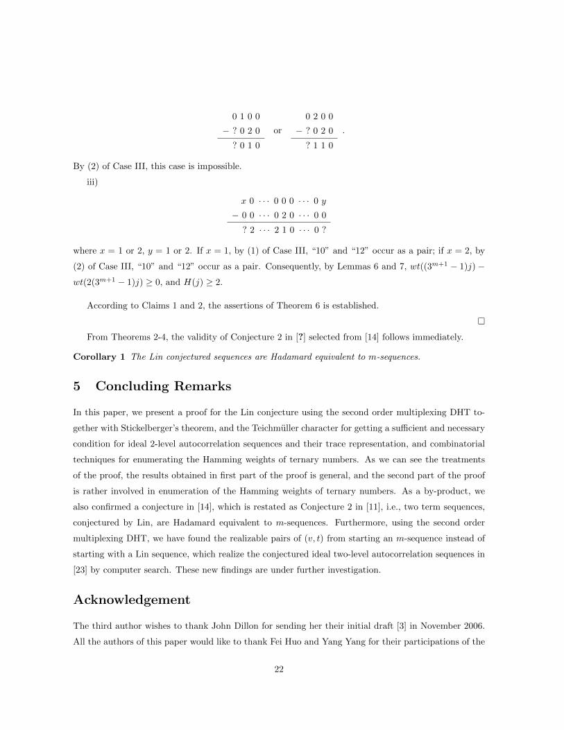
0 1 0 0
− ? 0 2 0
? 0 1 0
or
0 2 0 0
− ? 0 2 0
? 1 1 0
.
By (2) of Case III, this case is impossible.
iii)
x 0 · · · 0 0 0 · · · 0 y
− 0 0 · · · 0 2 0 · · · 0 0
? 2 · · · 2 1 0 · · · 0 ?
where x = 1 or 2, y = 1 or 2. If x = 1, by (1) of Case III, “10” and “12” occur as a pair; if x = 2, by
(2) of Case III, “10” and “12” occur as a pair. Consequently, by Lemmas 6 and 7, wt((3m+1 − 1)j)−
wt(2(3m+1 − 1)j) ≥ 0, and H(j) ≥ 2.
According to Claims 1 and 2, the assertions of Theorem 6 is established.
�
From Theorems 2-4, the validity of Conjecture 2 in [?] selected from [14] follows immediately.
Corollary 1 The Lin conjectured sequences are Hadamard equivalent to m-sequences.
5 Concluding Remarks
In this paper, we present a proof for the Lin conjecture using the second order multiplexing DHT to-
gether with Stickelberger’s theorem, and the Teichmuller character for getting a sufficient and necessary
condition for ideal 2-level autocorrelation sequences and their trace representation, and combinatorial
techniques for enumerating the Hamming weights of ternary numbers. As we can see the treatments
of the proof, the results obtained in first part of the proof is general, and the second part of the proof
is rather involved in enumeration of the Hamming weights of ternary numbers. As a by-product, we
also confirmed a conjecture in [14], which is restated as Conjecture 2 in [11], i.e., two term sequences,
conjectured by Lin, are Hadamard equivalent to m-sequences. Furthermore, using the second order
multiplexing DHT, we have found the realizable pairs of (v, t) from starting an m-sequence instead of
starting with a Lin sequence, which realize the conjectured ideal two-level autocorrelation sequences in
[23] by computer search. These new findings are under further investigation.
Acknowledgement
The third author wishes to thank John Dillon for sending her their initial draft [3] in November 2006.
All the authors of this paper would like to thank Fei Huo and Yang Yang for their participations of the
22
Waterloo Working Group for Attempting the Lin Conjecture in August, 2011, Waterloo [14], and their
tremendous contributions and help for many computational results toward the proof.
References
[1] K.T. Arasu. Sequences and arrays with desirable correlation properties.
arhiva.math.uniri.hr/NATO-ASI/abstracts/arasu.pdf, 2011.
[2] K.T. Arasu, J.F. Dillon, and K.J. Player, New p-ary sequences with ideal autocorrelation, Pre-
proceedings of Sequences and Their Applications (SETA 2004), pp. 1-5, 2004.
[3] K.T. Arasu, J.F. Dillon, and K.J. Player. Character sum factorizations yield perfect sequences,
Preprint, 2010.
[4] J. F. Dillon, Multiplicative difference sets via additive characters, Des., Codes, Cryptogr., vol. 17,
pp. 225-236, Sept. 1999.
[5] J.F. Dillon, New p-ary perfect sequences and dierence sets with Singer parameters, Proceedings of
Sequences and Their Applications, Discrete Math. Theor. Comput. Sci. (Lond.), Springer, London,
pp. 23-33, 2002.
[6] J. F. Dillon and H. Dobbertin, New cyclic difference sets with Singer parameters, Finite Fields
and Their Applications, vol. 10, 342-389, 2004.
[7] H. Dobbertin, Kasami power functions, permutation polynomials and cyclic difference sets, in
Difference Sets, Sequences and their Correlation Properties, ser. NATO Science Series, Series C:
Mathematical and Physical Sciences, A. Pott, P. V. Kumar, T. Helleseth, and D. Jungnickel, Eds.
Dordrecht, The Netherlands: Kluwer Academic, 1999, vol. 542, pp. 133-158.
[8] R. Evan, H.D.L. Hollman, C. Krattenthaler, and Q. Xiang, Gauss sums, Jacobi sums and p-ranks
of cyclic difference sets, Journal of Combinatorial Theory, Series A 87, No. 1, pp. 74-119, 1999.
[9] S. Golomb, Shift Register Sequences. Oakland, CA: Holden-Day, 1967. Revised edition: Laguna
Hills, CA: Aegean Park Press, 1982.
[10] S. W. Golomb and G. Gong, Signal Designs With Good Correlation: For Wireless Communi-
cations, Cryptography and Radar Applications. Cambridge, U.K.: Cambridge University Press,
2005.
[11] G. Gong, Character sums and polyphase sequence families with low correlation, DFT and ambi-
guity, to be appeared in Character Sums and Polynomials, A. Winterhof et al., Eds., De Gruyter,
23
Germany, pp. 1 - 43, 2013. Also appear as Technical Report, University of Waterloo, CACR
2012-21, http://cacr.uwaterloo.ca/techreports/2012/cacr2012-21.pdf.
[12] G. Gong, P. Gaal and S.W. Golomb, A suspected infinite class of cyclic Hadamard difference
sets, Proceedings of 1997 IEEE Information Theory Workshop, July 6-12, 1997, Longyearbyen,
Svalbard, Norway.
[13] G. Gong and S. W. Golomb, The Decimation-Hadamard transform of two-level autocorrelation
sequences, IEEE Trans. on Inform. Theory, vol. 48, No. 4, April 2002, pp. 853-865.
[14] G. Gong, T. Helleseth, H.G. Hu, F. Huo, and Y. Yang. On conjectured ternary 2-level autocorre-
lation sequences. Progress Report, August 2011.
[15] G. Gong, T. Helleseth, H. Hu, and A. Kholosha, “On the dual of certain ternary weakly regular
bent functions,” IEEE Trans. Inf. Theory, vol. 58, no. 4, pp. 2237-2243, Apr. 2012.
[16] T. Helleseth and G. Gong, New nonbinary sequences with ideal two-level autocorrelation functions,
IEEE Trans. Inf. Theory, vol. 48, no. 11, pp. 2868-2872, Nov. 2002.
[17] T. Helleseth, H. D. L. Hollmann, A. Kholosha, Z. Wang, and Q. Xiang, “Proofs of two conjectures
on ternary weakly regular bent functions,” IEEE Trans. Inf. Theory, vol. 55, no. 11, pp. 5272-5283,
Nov. 2009.
[18] T. Helleseth and P. V. Kumar, Sequences with low correlation, in Handbook of Coding Theory,
V. S. Pless and W. C. Huffman, Eds. Amsterdam, The Netherlands: Elsevier Science, 1998, pp.
1765-1853.
[19] T. Helleseth, P. V. Kumar, and H. Martinsen, A new family of ternary sequences with ideal
two-level autocorrelation function, Des., Codes Cryptogr., vol. 23, pp. 157-166, 2001.
[20] S. Lang, Cyclotomic Fields. New York: Springer-Verlag, 1978.
[21] R. Lidl and H. Niederreiter, Finite Fields. Reading, MA: Addison-Wesley, 1983, now distributed
by Cambridge Univ. Press.
[22] A. Lin, From cyclic Hadamard difference sets to perfectly balanced sequences, Ph.D. Thesis,
University of Southern California, Los Angeles, 1998.
[23] M. Ludkovski and G. Gong, New families of ideal 2-level autocorrelation ternary sequences from
second order DHT, Proceedings of the Second International Workshop on Coding and Cryptogra-
phy, January 8-12, 2001, Paris, France, pp. 345-354.
24
[24] A. Maschietti, Difference sets and hyperovals, Des., Codes, Cryptogr., vol. 14, pp. 89-98, 1998.
[25] J. S. No, H. Chung, and M. S. Yun, Binary pseudorandom sequences of period 2m − 1 with ideal
autocorrelation generated by the polynomial zd + (z + 1)d, IEEE Trans. Inform. Theory, vol. 44,
pp. 1278-1282, May 1998.
[26] J. S. No, S. W. Golomb, G. Gong, H. K. Lee, and P. Gaal, New binary pseudo-random sequences
of period 2n − 1 with ideal autocorrelation, IEEE Trans. Inform. Theory, vol. 44, pp. 814-817,
Mar. 1998.
[27] M. K. Simon, J. K. Omura, R. A. Sholtz, and B. K. Levitt, Spread Spectrum Communications.
Rockville, MD: Computer Sci., 1985, vol. 1.
[28] Q. Xiang, On balanced binary sequences with two-level autocorrelation functions, IEEE Trans.
on Inform. Theory, Vol. 44, No. 7, November 1998, pp. 3153-3156.
[29] N. Y. Yu and G. Gong, Realization of decimation-Hadamard transform for binary generalized
GMW sequences, Proceedings of Workshop on Coding and Cryptography (WCC2005), pp. 127-
136, Bergen, Norway, March 14-18. 2005.
[30] N.Y. Yu and G. Gong, Multiplexing realizations of the decimation-Hadamard transform of two-
level autocorrelation sequences, Proceedings of Coding and Cryptology, LNCS, volume 5557, pages
248- 258, Springer-Verlag, 2009.
25