Embed Size (px)
Citation preview
MSc in Data Warehousing and Data Mining University of Greenwich
The Progress Report for a dissertation to be submitted in partial
fulfilment of University of Greenwich Master Degree
MSc Project Title
An investigation into consolidating information from heterogenic Databases using Data
Warehousing and Data Visualisation Techniques for Raiyan Telecom Carrier Limited (RTCL).
Name: Mohammad Abdus Samad
Student ID: 000655556
Programme of Study: MSc Data Warehousing & Data Mining
Final Report
Project Hand in Date: 30-Jan-2012
Supervisor: Elena Teodorescu
Word Count: 14682
MSc in Data Warehousing and Data Mining University of Greenwich
Page 1 of 133
An investigation into consolidating information from heterogenic Databases using
Data Warehousing and Data Visualisation Techniques for RTCL
Computing & Mathematical Sciences, University of Greenwich, 30 Park Row, Greenwich, UK.
(Submitted 30 Jan 2012)
ABSTRACT
Businesses have various systems or software for doing its day to day actions. Businesses can have
system for trading its products, handling its supply and suppliers, handling its staff, handling its
finance and other resources. All of these systems have essential data. Businesses have core data
available for these systems, and then the next and most significant issue is how to use the data?
Most of businesses run by different type of software. So the organization data are scattered. How
data can be used to take strategic resolution to increase performance? At this phase Data
Warehouse and Business intelligence comes in to picture to transform data in to knowledge and
intelligence to enhance performance and financial planning. Data Warehouse contains the all
historical data in one organization with the integrated from all data sources. For generating BI report
or applying data mining data warehouse supply the previous business data. Business intelligence
responses to the management of the company strategic query such as which are the business’s most
money-spinning products and customers, and what influence a specific event may have on cash flow
and earnings in a next five years. BI provides the small knowledge to small business owners which
are the a features driving most profit to the business and to do what-if analysis on the basis of
scenarios such as inaugural of a new branch, developing and introduction a new product,
penetrating new markets etc. Analysis tools of the BI deliver users to answer the truly hard
questions of business. The tools are giving consistent data which provides a real truth of a current
situation. Business performance is observed and measured by the right initiatives that can be
confirmed by using the BI.
Keywords: ETL; Data warehouse design; Data Visualisation; ASP.NET; C#; Silverlight.

MSc in Data Warehousing and Data Mining University of Greenwich
Page 2 of 133
Acknowledgements
I would especially like to thank Ms Elena Teodorescu for agreeing to be my supervisor
and for her consistent advice, feedback, guidance and support throughout the
lifecycle of this MSc project.
I want to thank both Ms Elena Teodorescu and Ms Gill Windall for agreeing to have
the project demonstration on the schedule day.
I would also thank all my Respectable Professors of Greenwich University for giving
me guidance, encouragement for developing my skills and knowledge.
MSc in Data Warehousing and Data Mining University of Greenwich
Page 3 of 133
Table of Contents Chapter 1 ................................................................................................................................................. 8
Introduction ........................................................................................................................................ 8
1.1 Overview ................................................................................................................................... 8
1.2 Problem statement in existing system ...................................................................................... 8
1.3 Building Data Warehouse and Data Visualisation for BI as a Solution ..................................... 2
1.4 Problem solving step ............................................................................................................... 2
Chapter 2 ................................................................................................................................................. 3
Literature Review ................................................................................................................................ 3
2.1 Overview ................................................................................................................................... 3
2.2 Data Warehousing Functions .................................................................................................... 3
2.3 Methodology Review ................................................................................................................ 3
2.3.1 Top down Approach: Enterprise Data Warehouse ................................................................ 4
2.3.2 Bottom up Approach: Data Mart ........................................................................................... 6
2.3.3 Hybrid Approach .................................................................................................................... 7
2.4 Operational Databases vs Data Warehouses ............................................................................ 8
2.5 Multidimensional Modelling ..................................................................................................... 9
2.5.1 OLAP Operation Description ................................................................................................ 10
2.6 Data Warehouse Schema Designs .......................................................................................... 11
2.6.1 Star Schema ......................................................................................................................... 11
2.6.2 Snowflake Schema ............................................................................................................... 12
2.6.3 Starflake Schema .................................................................................................................. 14
2.7 OLAP Architecture ................................................................................................................... 15
2.7.1 Multidimensional OLAP ....................................................................................................... 16
2.7.2 Relational OLAP .................................................................................................................... 17
2.7.3 Hybrid OLAP ......................................................................................................................... 17
2.8 ETL role in Data Warehousing and reporting .......................................................................... 17
2.8.1 Comparison between various ETL tools ............................................................................... 18
2.8.2 Pentaho Kettle ETL Tools ..................................................................................................... 19
2.8.2.1 Enterprise-Class ETL .......................................................................................................... 19
2.8.2.2 Common Use Cases ........................................................................................................... 19
2.9 Data Visualization ................................................................................................................... 20
2.10 Summary ............................................................................................................................... 21
Chapter 3 ............................................................................................................................................... 22
MSc in Data Warehousing and Data Mining University of Greenwich
Page 4 of 133
Requirement analysis and design ..................................................................................................... 22
3.1 Overview ................................................................................................................................. 22
3.2 Software Process Model ......................................................................................................... 22
3.3 Using Tools .............................................................................................................................. 23
3.3.1 Back End ............................................................................................................................... 23
3.3.2 Front End .............................................................................................................................. 23
3.3.3 Languages............................................................................................................................. 23
3.3 Existing system ........................................................................................................................ 24
3.3.1 Voipswitch MYSQL Database: .............................................................................................. 26
3.3.2 Sippy Oracle Database: ........................................................................................................ 27
3.4 Design Data Warehousing and Reporting System .................................................................. 27
3.4.1 Staging Area Design ............................................................................................................. 28
3.4.1.1 Stage Voipswitch (MYSQL) ................................................................................................ 28
3.4.1.2 Stage Sippy (ORACLE) ........................................................................................................ 28
3.4.2 Data warehouse design decisions ........................................................................................ 29
3.4.3 Proposed data visualisation reporting architecture ............................................................ 30
3.5 What new visualisation report system propose ..................................................................... 31
Chapter 4 ............................................................................................................................................... 33
Implement Data Warehouse ............................................................................................................. 33
4.1 Overview ................................................................................................................................. 33
4.2 Technology used for implementation ..................................................................................... 33
4.2.1 ETL Tool – Pentaho ............................................................................................................... 33
4.3 Implement Data Warehouse ................................................................................................... 34
4.3.1 Dimension Table .................................................................................................................. 34
4.3.2 Dimensional hierarchy ......................................................................................................... 36
4.3.1 Fact Table ............................................................................................................................. 36
4.3.2. Partitioning .......................................................................................................................... 37
Types of partitioning ..................................................................................................................... 38
4.3.3 Materialized View ................................................................................................................ 38
4.3.4 Examining the performance of the materialized view ......................................................... 39
4.3.5 Indexing ................................................................................................................................ 40
4.3 Flow chart of the system development .................................................................................. 41
4.4 Phase 1: ETL Process ............................................................................................................... 41
4.4.1 Data warehouse data loading by Pentaho ........................................................................... 44
MSc in Data Warehousing and Data Mining University of Greenwich
Page 5 of 133
4.4.2 Data warehouse data loading by procedures ...................................................................... 46
Chapter 5 ............................................................................................................................................... 47
Implement Data Visualisation for BI ................................................................................................. 47
5.1 Overview ................................................................................................................................. 47
5.2.1 ASP.NET Application 2010 (C#) ............................................................................................ 47
5.2.2. Entity Framework ................................................................................................................ 47
5.2.2 Silverlight Tool Kit ................................................................................................................ 48
5.3 Phase 1: Finalizing reports ...................................................................................................... 48
5.4 Phase 3: Web Application design and development .............................................................. 49
Chapter 6 ............................................................................................................................................... 53
Testing and Comparison ................................................................................................................... 53
6.1 Overview ................................................................................................................................. 53
6.2 Test Cases ................................................................................................................................ 53
6.3. Comparison of the developed system with other Tools ........................................................ 54
Chapter 7 ............................................................................................................................................... 56
Evaluation and Future work .............................................................................................................. 56
7.1 Overview ................................................................................................................................. 56
7.2 Phase 1 .................................................................................................................................... 56
7.3 Phase 2 .................................................................................................................................... 56
7.4 Phase 3 .................................................................................................................................... 56
7.5 Phase 4 .................................................................................................................................... 57
Chapter 8 ............................................................................................................................................... 58
Conclusion ......................................................................................................................................... 58
8.1 General conclusion .................................................................................................................. 58
8.2 Personal Experience ................................................................................................................ 58
References ............................................................................................................................................ 59
Appendix A: ........................................................................................................................................... 63
Confidential Disclosure Agreement .............................................................................................. 63
Appendix B ............................................................................................................................................ 64
Voipswitch MYSQL Database’s Table Description ........................................................................ 64
Appendix C ............................................................................................................................................ 68
Sippy Oracle Database’s Table Description................................................................................... 68
Appendix D ............................................................................................................................................ 71
Dimension and FACT Table Analysis ................................................................................................. 71
MSc in Data Warehousing and Data Mining University of Greenwich
Page 6 of 133
Employees Dimension ................................................................................................................... 71
Locations Dimension ..................................................................................................................... 72
Customer Dimension .................................................................................................................... 73
Calls Fact ....................................................................................................................................... 74
Payment Fact: ............................................................................................................................... 75
Appendix E ............................................................................................................................................ 76
Staging Area Cleansing Procedure ................................................................................................ 76
Appendix F ............................................................................................................................................ 81
Creation Script for Table, Dimensional hierarchy and Fact Table................................................. 81
Appendix G ............................................................................................................................................ 87
Procedure for Loading Data into the Data Warehouse ................................................................ 87
Appendix H ............................................................................................................................................ 98
Indexing for data warehouse ........................................................................................................ 98
APPENDIX I .......................................................................................................................................... 100
Materialized View Creation Code ............................................................................................... 100
APPENDIX J .......................................................................................................................................... 106
Testing of the system .................................................................................................................. 106
APPENDIX K ......................................................................................................................................... 109
ASP.NET CODE ............................................................................................................................. 109
Appendix L ........................................................................................................................................... 119
Report Screen Shot ..................................................................................................................... 119
Appendix M ......................................................................................................................................... 123
Subject-Oriented Data ................................................................................................................ 123
Integrated Data ........................................................................................................................... 123
Time-Variant Data ....................................................................................................................... 124
Non-Volatile Data ........................................................................................................................ 124
Entity Relationship Schema ........................................................................................................ 125
MSc in Data Warehousing and Data Mining University of Greenwich
Page 7 of 133
List of Tables Table 2.1 Difference between an Operational Database and a Data Warehouse 08
Table 2.2: ETL Tools Comparison 18
Table 3.1: Staging Area Table Name for Voipswitch 28
Table 3.2: Staging Area table name for Sippy 28
Table 3.3: shows the finalized reports with its description. 32
Table 4.1: Materialized View Table 38
Table 4.2 Index Table 40
Table 4.3: Cleaning procedure table 44
Table 4.4: Data warehouse load procedure 44
Table 6.1: Test Cases 54
List of Figures Figure 2.1: Top down approach (Enterprise data warehouse). 05
Figure 2.2: Bottom up approach. 06
Figure 2.3: Multidimensional data cube. 09
Figure 2.4: Star Schema 12
Figure 2.5: Snowflake schema 13
Figure 2.6: Starflake schema with one fact and two dimensions that share an outrigger. 15
Figure 2.7: Data warehouse and OLAP servers 16
Figure 2.8: Pentaho Architecture. 20
Figure 2.9: Show Visualisation technique with chart for sales in different region 21
Figure 3.1: Spider Model 23
Figure 3.2: RTCL Existing System 24
Figure 3.3: Voipswitch Database Schema. 26
Figure 3.4: Sippy Database Schema. 27
Figure 3.5: Data Warehouse Star Schema. 30
Figure 3.6: Proposed Data Warehousing and Data Visualisation or Reporting System Architecture 31
Figure 4.1: EXPLAIN PLAN FOR “MV_TopUsagesDest” Materialized View’s Query. 39
Figure 4.2: Development Process Flow Chart 41
Figure 4.3: Extract MYSQL Vendors table to Stage Area Oracle STG_VS_Vendors Table. 41
Figure 4.4: Pentaho Connection, Input and Output Table. 42
Figure 4.5: Extraction of MYSQL database to Oracle Staging Area using Pentaho Job 42
Figure 4.6: Extraction of Oracle Sippy database to Oracle Staging Area Schema using Pentaho Job 43
Figure 4.7: Job for extraction both data source to Staging Area. 43
Figure 4.8: Customer Dimension Table Mapping. 44
Figure 4.9: Job for loading data into all dimension tables 45
Figure 4.10: Job for loading data into all fact tables 45
Figure 4.11: Job for loading data into all dimension and fact tables with other two jobs 45
Figure 5.1: List of Report 48
Figure 5.2: Login Page 49
Figure 5.3: Figure 5.3: Entity Data Model Wizard 50
Figure 5.4: Dashboard in greyscale 51
Figure 5.5: Usages by Yearly 52
Figure 5.6: To Sales by Month in Different Year. 52
MSc in Data Warehousing and Data Mining University of Greenwich
Page 8 of 133
Chapter 1
Introduction
1.1 Overview
Nowadays in the organizations for strategic decision making transactional and operational databases
plays a significant role. Since data warehousing technology emerged over a decade ago, it has
revolutionised the business decision support system by enabling better and faster strategic decision
making. Each and every organization has its own requirements of reports about its data. For
example, retail sales company has its own reports (i.e. product performance reports, staff
performance reports), similarly educational institutions has reports (i.e. students performance
reports, staff performance report, contractor performance reports etc.). Before few decades
organizations were gathering these requirements using straightforward Microsoft Excel, spreadsheet
and traditional file processing. But this simple reporting software does not work as the amount of
data grows with the growth of the company. So the spreadsheet and ordinary file processing were
not capable to handle the size and amount of data. The main objectives of this study are to
investigate the data warehouse designs and show the reporting system. There is clear evidence from
the literature that this topic area has a pivotal role in data warehousing.
1.2 Problem statement in existing system
In this Project I am investigation study with implement Data Warehouse and Business Intelligence solution
for a Telecommunications Company. RTCL is using three different billing systems. Initially, they started
their business with Voipswitch billing system then as per company need they purchased another one
billing systems from other companies for other advantages. They are facing problem to generate report
because of using different systems. Currently, they are also using some old reporting systems, which
don’t generate analytical reports. So, now they need Business Intelligence solution to replace the old
reporting systems. This will help them in forecasting and seeing the trends, which in turn will help in
improving the business. The aim of the project is to offer data warehousing solution for VOIP
Telecommunications Sector. It will provide Decision Support System by offering BI Analysis and analytical
reports to the Management by using visualisation of VOIP Telecommunications Sector. The project offers
solution for BI analytics for billing system and financial system in VOIP Telecommunications Sector. The
project proposes that the integration of disparate data marts from different sources will be maintained in
particular time interval or real-time, providing a single, canonical. This can be accessed through the
presentation layer i.e. the reports such as different graphical report.
MSc in Data Warehousing and Data Mining University of Greenwich
Page 2 of 133
1.3 Building Data Warehouse and Data Visualisation for BI as a Solution
The main aim of developing this system is to build the data warehouse and provide productive BI
reporting Solution to the organization. For BI reporting system to get data build the data warehouse
with different data source and finally develop the BI report by using Silverlight with ASP.NET.
Business intelligence focuses on the three factors such as The Right Information, The Right Person
and The Right Time. The Right Information means only that information that is useful to the decision
makers and that should be acted upon. The Right Person means the person who has the knowledge
to process the information which needs to be act upon. The Right Time means the right period in
which the necessary action must be taken that include sending an email, mobile phone text alert to
make sure that the information is delivered on time.
1.4 Problem solving step
This purpose is accomplished through subsequent phases. The next chapters of this project are
literature review, requirement analysis, design and development. In the literature review, potential
requirements of the BI reporting system for an organizations, the critical comparison of the existing
ETL and BI reporting tools are discussed. In requirement analysis and design, the existing system and
the requirement of the user, the data warehouse design and architecture of the new system are
discussed. In the development part, the methods and technologies for implementation of the system
are discussed. At last the system is tested with appropriate testing procedures and the
methodologies are discussed.
MSc in Data Warehousing and Data Mining University of Greenwich
Page 3 of 133
Chapter 2
Literature Review
2.1 Overview
The objective of this literature review is the theoretical analysis of data warehousing methodology
derived through research on data warehousing research papers and journals. Data warehouses can
be considered as a development of management information system (Inmon 1996). In this research
paper, we make a summary of this state of the art, propose design approach and point out research
problems in the areas of data warehouse modelling and designing, data cleansing, Extraction
Transformation and Loading (ETL) and metadata management and Implement the Data Visualisation.
2.2 Data Warehousing Functions
Since the past years, the data warehouse system has grown into a vital ‘state of the art’ innovative
technology for most corporations. Various functions of the data warehouse which have contributed
to its achievement are: users have the skill to invoke analysis, planning and decision support
applications from the decision layer (data warehouse) as a substitute of the operational database
(Saharia & Babad 2000); better complex query performance ; facilities of ad hoc queries that
combine and associate data (Huang et al 2005, Saharia & Babad 2000, Datta & Thomas 1999) ; the
incorporation of multiple distributed heterogeneous databases into a single data warehouse
repository (Singhal 2004, Theodoratos et al 2001) and accommodations for data mining from
comprehensive, summarised and historical data (Inmon 1996).
In spite of its innovation, data warehousing technology is always changing to keep pace with
research and development in modern science. Data warehousing has matured so much over the past
few decades (Priebe and Pernul 2000). Nowadays, many big corporate companies have data
warehousing technologies to vie in this dynamic and extremely competitive globalise market.
2.3 Methodology Review
There is a debate within the data warehousing community about to the technique a data warehouse
is designed and implemented. Some of these communities of thoughts are: top down approach
(Enterprise data warehouse), bottom up approach (Data Marts) and a hybrid approach. The
succeeding sections of this chapter are a critical analysis of these various approaches to data
warehousing and the differences and similarities between the data warehouse architectures.
MSc in Data Warehousing and Data Mining University of Greenwich
Page 4 of 133
2.3.1 Top down Approach: Enterprise Data Warehouse
One data warehouse definition that is so in vogue comes from Inmon (1992) who is familiar as the
“father of the data warehouse”:
“A data warehouse is a subject-oriented, integrated, time-variant, non-volatile collection of data in
support of management’s decision making process”.
Inmon’s data warehouse characteristics
i. Separate
ii. Available
iii. Integrated
iv. Time stamped
v. Non-volatile
vi. Accessible
There is described some characteristics of data warehousing technology on the basis of these
definitions in Appendix M.
The top down approach of building data warehouse is mostly data driven. The main disadvantages
are: time consuming to build, high risk of failure, needs high level of cross functional skills. Therefore
this approach could be hazardous because lack of experienced professional team.
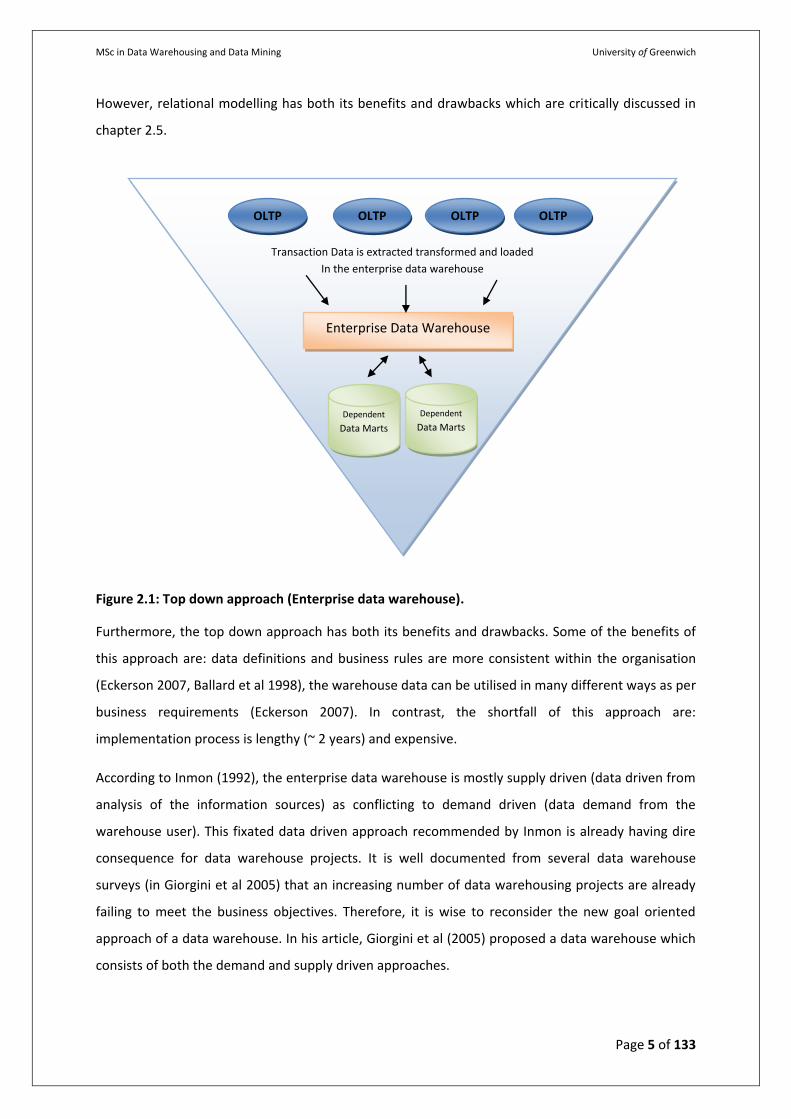
Inmon’s enterprise data warehouse architecture as shown in Figure 2.1 has been labelled as the top
down approach by many experts. This approach is based on the enterprise data warehouse being a
physically distinct entity instead of a collection of data marts. Transaction data from the Online
Transaction Processing (OLTP) source systems (operational databases) is extracted, transformed and
loaded into the Enterprise data warehouse. Once the enterprise data warehouse has been
implemented all the users within the enterprise can be serviced by dependent data marts (e.g.
finance, sales, marketing, and accounting).
In the enterprise data warehouse, data is stored in third normal form and the structure and content
of the data warehouse is dictated by the enterprise instead of departmental data requirements
(Drewek, 2005). Not surprisingly, Inmon favours the relational model which is in third normal form.
MSc in Data Warehousing and Data Mining University of Greenwich
Page 5 of 133
However, relational modelling has both its benefits and drawbacks which are critically discussed in
chapter 2.5.
Figure 2.1: Top down approach (Enterprise data warehouse).
Furthermore, the top down approach has both its benefits and drawbacks. Some of the benefits of
this approach are: data definitions and business rules are more consistent within the organisation
(Eckerson 2007, Ballard et al 1998), the warehouse data can be utilised in many different ways as per
business requirements (Eckerson 2007). In contrast, the shortfall of this approach are:
implementation process is lengthy (~ 2 years) and expensive.
According to Inmon (1992), the enterprise data warehouse is mostly supply driven (data driven from
analysis of the information sources) as conflicting to demand driven (data demand from the
warehouse user). This fixated data driven approach recommended by Inmon is already having dire
consequence for data warehouse projects. It is well documented from several data warehouse
surveys (in Giorgini et al 2005) that an increasing number of data warehousing projects are already
failing to meet the business objectives. Therefore, it is wise to reconsider the new goal oriented
approach of a data warehouse. In his article, Giorgini et al (2005) proposed a data warehouse which
consists of both the demand and supply driven approaches.
Transaction Data is extracted transformed and loaded
In the enterprise data warehouse
Dependent
Data Marts
Dependent
Data Marts
Enterprise Data Warehouse
OLTP OLTP OLTP OLTP
MSc in Data Warehousing and Data Mining University of Greenwich
Page 6 of 133
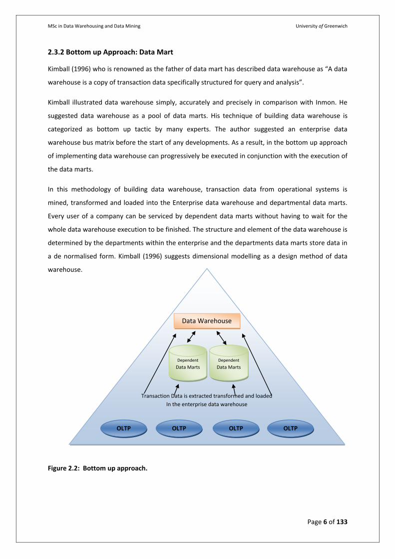
2.3.2 Bottom up Approach: Data Mart
Kimball (1996) who is renowned as the father of data mart has described data warehouse as “A data
warehouse is a copy of transaction data specifically structured for query and analysis”.
Kimball illustrated data warehouse simply, accurately and precisely in comparison with Inmon. He
suggested data warehouse as a pool of data marts. His technique of building data warehouse is
categorized as bottom up tactic by many experts. The author suggested an enterprise data
warehouse bus matrix before the start of any developments. As a result, in the bottom up approach
of implementing data warehouse can progressively be executed in conjunction with the execution of
the data marts.
In this methodology of building data warehouse, transaction data from operational systems is
mined, transformed and loaded into the Enterprise data warehouse and departmental data marts.
Every user of a company can be serviced by dependent data marts without having to wait for the
whole data warehouse execution to be finished. The structure and element of the data warehouse is
determined by the departments within the enterprise and the departments data marts store data in
a de normalised form. Kimball (1996) suggests dimensional modelling as a design method of data
warehouse.
Figure 2.2: Bottom up approach.
Transaction Data is extracted transformed and loaded
In the enterprise data warehouse
Data Warehouse
Dependent
Data Marts
Dependent
Data Marts
OLTP OLTP OLTP OLTP
MSc in Data Warehousing and Data Mining University of Greenwich
Page 7 of 133
The bottom up approach also has some advantages and disadvantages as well. Some of the
advantages Ponniah (2001, p.26) of this method include:
Faster and easier execution of manageable pieces
Faster return on investment and proof of concept
Less risk of failure than top down approach
Can schedule important data mart first as it is inherently incremental
Cheaper than any other data warehouse design approach as it is less complex designing
On the contrary, this method has following drawbacks Ponniah (2001, p.27) in the implementation
stage.
Each data marts has its individual contracted outlook of data
Incorporating data within data marts and data warehouse can be intricate as extra
dimension and fact table has to impose to do the integration.
In this method, data rests split in various individual data marts. Hence, individual data
marts will not be supportive to the overall necessities of the whole organisations.
As integrating the data marts is easier approach than starting the data warehouse at enterprise
level. At the moment using bottom up approach because I am starting with billing systems for RTCL.
Company has planned to make an enterprise wide data warehouse. But it is like a prototype, so
starting with the billing system. Later depending upon the success of project, an enterprise wide
data warehouse will be implemented.
2.3.3 Hybrid Approach
The hybrid method was invented by data warehouse specialists and it includes both Inmon and
Kimball approaches in order to attain an optimal design. This method is often called as the (Ballard
et al 1998) “combined approach” and more lately as (Mailvaganam 2004) the “third way” of data
warehouse design. The goal of this method is balanced on both the advantage of the top down and
bottom up method in the implementation of the data warehouse. The implementation necessitates
the development of the enterprise data warehouse in a short period of time before the deployment
of dependent data marts. In this method, the data marts capitalise normalised data and dimensional
modelling. The main advantages of this method are: the pace of implementation of the bottom up
method aggregated with the enforced integration characteristics of the top down approach
(Eckerson 2007).
MSc in Data Warehousing and Data Mining University of Greenwich
Page 8 of 133
Nevertheless, this method is not resistant to disadvantages which include: it is comparatively new
and therefore it has not been extensively examined by the research community and in practicality it
is relatively complex to put on implementation.
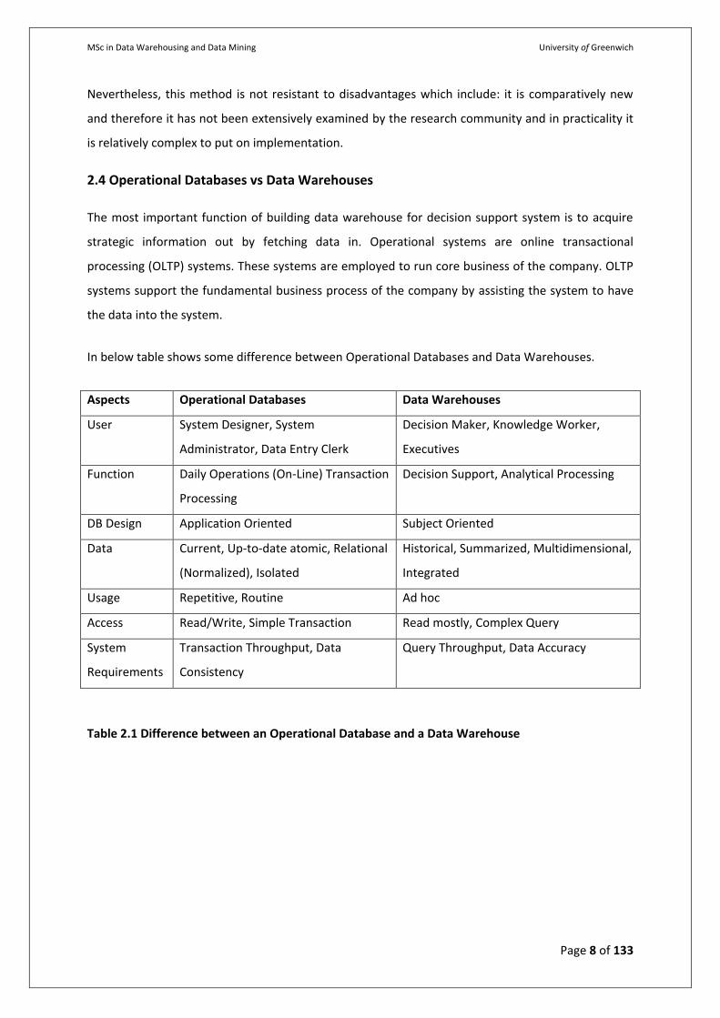
2.4 Operational Databases vs Data Warehouses
The most important function of building data warehouse for decision support system is to acquire
strategic information out by fetching data in. Operational systems are online transactional
processing (OLTP) systems. These systems are employed to run core business of the company. OLTP
systems support the fundamental business process of the company by assisting the system to have
the data into the system.
In below table shows some difference between Operational Databases and Data Warehouses.
Aspects Operational Databases Data Warehouses
User System Designer, System
Administrator, Data Entry Clerk
Decision Maker, Knowledge Worker,
Executives
Function Daily Operations (On-Line) Transaction
Processing
Decision Support, Analytical Processing
DB Design Application Oriented Subject Oriented
Data Current, Up-to-date atomic, Relational
(Normalized), Isolated
Historical, Summarized, Multidimensional,
Integrated
Usage Repetitive, Routine Ad hoc
Access Read/Write, Simple Transaction Read mostly, Complex Query
System
Requirements
Transaction Throughput, Data
Consistency
Query Throughput, Data Accuracy
Table 2.1 Difference between an Operational Database and a Data Warehouse
MSc in Data Warehousing and Data Mining University of Greenwich
Page 9 of 133
2.5 Multidimensional Modelling
In data warehousing, the two significant designs techniques which are frequently used are: Entity
Relationship Modelling (ER) and dimensional modelling (Jones & Song 2005, Sen & Sinha 2005).
Multidimensional modelling is principally emploed for the development of data marts. Nevertheless,
ER modelling is most often used in operational database and enterprise data warehouse designs.
Both these vying approaches for organising data within a data warehouse have their advantages and
disadvantages. Entity relationship modelling is critically illustrated in Appendix M. This section is a
critical assessment of the multidimensional modelling technique which is used over rest of this
report.
The multidimensional modelling concept and framework was first brought in by Kimball (in Kimball
et al 1998). The authors illustrate this as an alternative data model to the ER model. Dimensional
schema is a generic term used in this investigative study to collectively refer to the star schema,
snowflake schema and starflake schema. The key advantages of the dimensional model are (Dash &
Agarwal 2001) the ease of the presented data format and the superior performance of the data
warehouse system. Furthermore, the advantages of dimensional modelling are the disadvantage of
ER modelling.
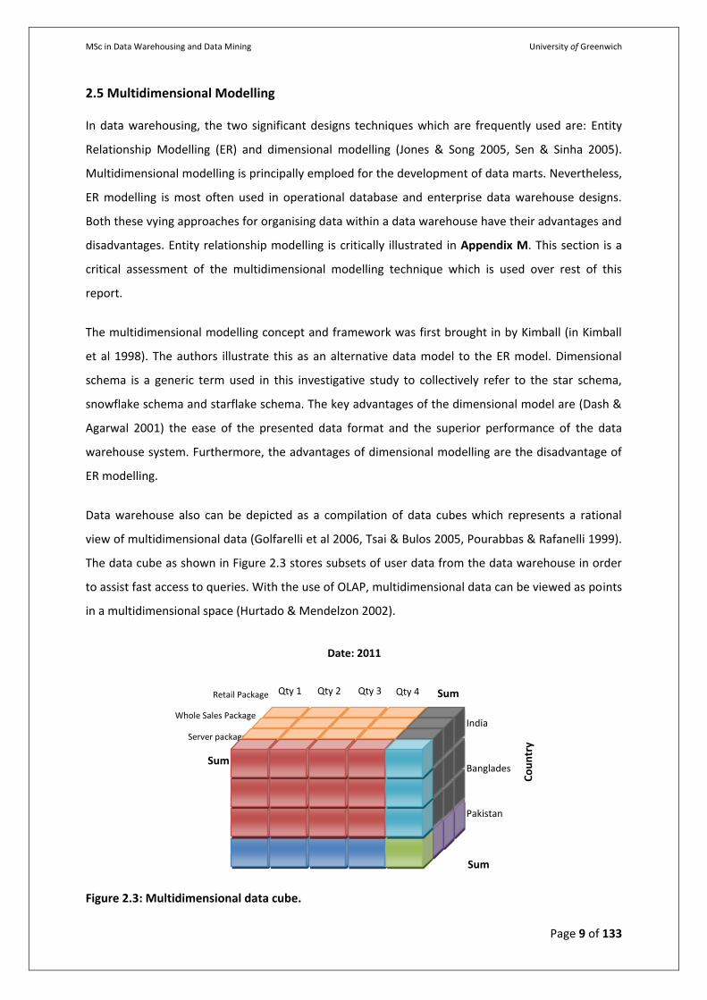
Data warehouse also can be depicted as a compilation of data cubes which represents a rational
view of multidimensional data (Golfarelli et al 2006, Tsai & Bulos 2005, Pourabbas & Rafanelli 1999).
The data cube as shown in Figure 2.3 stores subsets of user data from the data warehouse in order
to assist fast access to queries. With the use of OLAP, multidimensional data can be viewed as points
in a multidimensional space (Hurtado & Mendelzon 2002).
Figure 2.3: Multidimensional data cube.
Qty 3 Qty 4 Qty 1 Qty 2
Pakistan
Bangladesh
India
Sum
Sum
Server package
Sum
Whole Sales Package
Retail Package
Co
un
try
Date: 2011
MSc in Data Warehousing and Data Mining University of Greenwich
Page 10 of 133
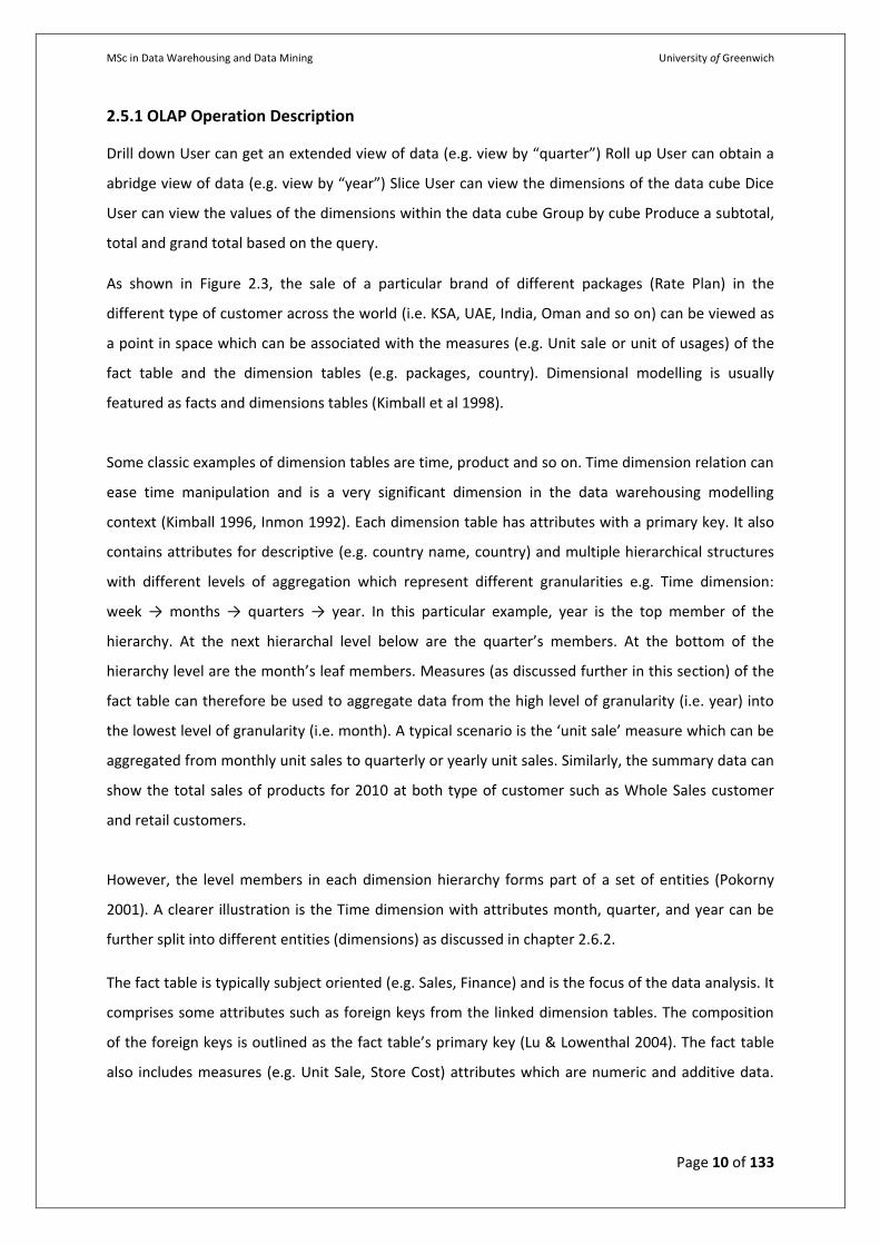
2.5.1 OLAP Operation Description
Drill down User can get an extended view of data (e.g. view by “quarter”) Roll up User can obtain a
abridge view of data (e.g. view by “year”) Slice User can view the dimensions of the data cube Dice
User can view the values of the dimensions within the data cube Group by cube Produce a subtotal,
total and grand total based on the query.
As shown in Figure 2.3, the sale of a particular brand of different packages (Rate Plan) in the
different type of customer across the world (i.e. KSA, UAE, India, Oman and so on) can be viewed as
a point in space which can be associated with the measures (e.g. Unit sale or unit of usages) of the
fact table and the dimension tables (e.g. packages, country). Dimensional modelling is usually
featured as facts and dimensions tables (Kimball et al 1998).
Some classic examples of dimension tables are time, product and so on. Time dimension relation can
ease time manipulation and is a very significant dimension in the data warehousing modelling
context (Kimball 1996, Inmon 1992). Each dimension table has attributes with a primary key. It also
contains attributes for descriptive (e.g. country name, country) and multiple hierarchical structures
with different levels of aggregation which represent different granularities e.g. Time dimension:
week → months → quarters → year. In this particular example, year is the top member of the
hierarchy. At the next hierarchal level below are the quarter’s members. At the bottom of the
hierarchy level are the month’s leaf members. Measures (as discussed further in this section) of the
fact table can therefore be used to aggregate data from the high level of granularity (i.e. year) into
the lowest level of granularity (i.e. month). A typical scenario is the ‘unit sale’ measure which can be
aggregated from monthly unit sales to quarterly or yearly unit sales. Similarly, the summary data can
show the total sales of products for 2010 at both type of customer such as Whole Sales customer
and retail customers.
However, the level members in each dimension hierarchy forms part of a set of entities (Pokorny
2001). A clearer illustration is the Time dimension with attributes month, quarter, and year can be
further split into different entities (dimensions) as discussed in chapter 2.6.2.
The fact table is typically subject oriented (e.g. Sales, Finance) and is the focus of the data analysis. It
comprises some attributes such as foreign keys from the linked dimension tables. The composition
of the foreign keys is outlined as the fact table’s primary key (Lu & Lowenthal 2004). The fact table
also includes measures (e.g. Unit Sale, Store Cost) attributes which are numeric and additive data.
MSc in Data Warehousing and Data Mining University of Greenwich
Page 11 of 133
The measures are important and they are used to calculate quantitative data analysis for the
organisation (Bonifati et al 2001).
The investigative data warehouse schemata (star schema, snowflake schema and starflake schema)
are critically reviewed in the next section of this chapter.
2.6 Data Warehouse Schema Designs
The subsequent sections of this chapter present a thorough critical analysis of four data warehouse
designs: ER schema, star schema, snowflake schema and starflake schema.
Nevertheless, the data warehouse designs are not at all a comprehensive list of schemata available.
Regrettably, due to space limitations other data warehouse designs have not been assessed in
depth. Despite the fact that there is a lack of sufficient research in data warehouse designs some
vital works have been published over the last decade which merits some critical evaluation.
The researchers (in Golfarelli and Rizzi 1998) offered a Dimensional Fact Model (DFM) which can be
employed to originate data warehouse schema from ER schema of data sources (operational
databases). This is a decent pace forward in the arena of data warehouse design. Nonetheless, the
DFM framework has restrictions as the data sources with non ER schema might not be utilised.
Other data warehouse schemata faced within the literature but not judgmentally analysed are the:
Multi-star schema (in Krippendorf & Song 1997, Poe 1996); Fact constellation schema (in Kimball
1996); StarER (in Tryfona et al 1999) and MultiDim ER model (in Malinowski & Zimanyi 2005).
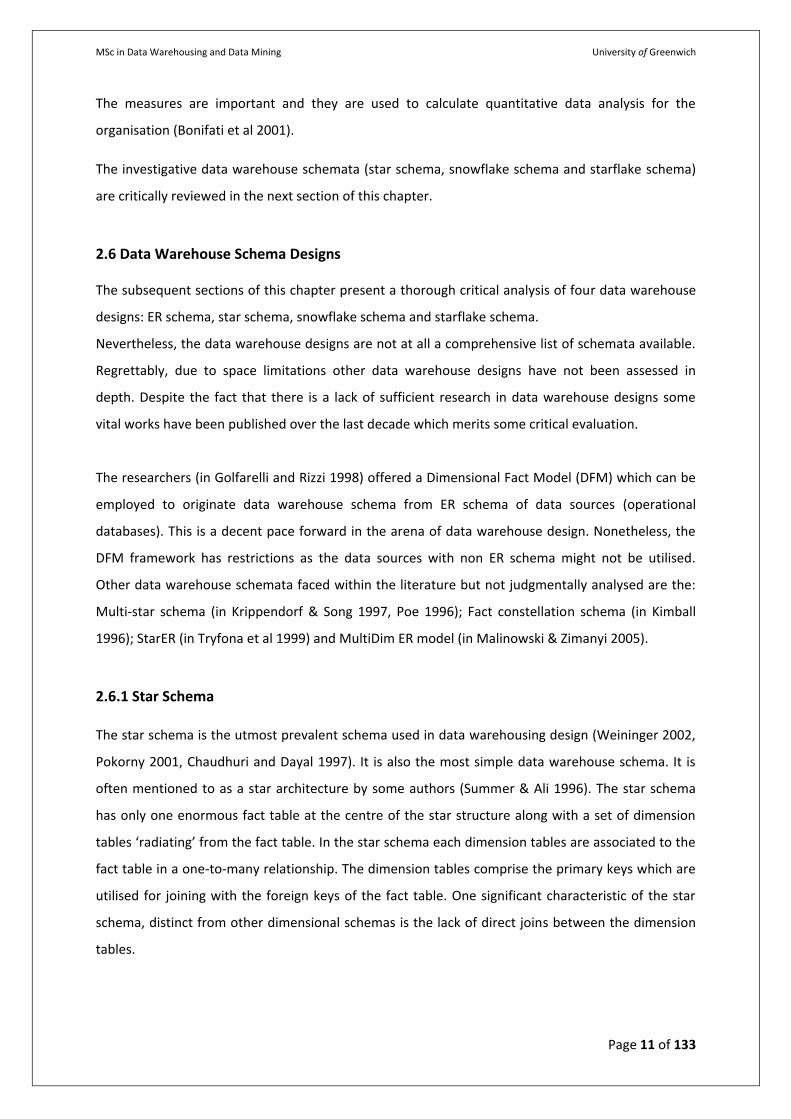
2.6.1 Star Schema
The star schema is the utmost prevalent schema used in data warehousing design (Weininger 2002,
Pokorny 2001, Chaudhuri and Dayal 1997). It is also the most simple data warehouse schema. It is
often mentioned to as a star architecture by some authors (Summer & Ali 1996). The star schema
has only one enormous fact table at the centre of the star structure along with a set of dimension
tables ‘radiating’ from the fact table. In the star schema each dimension tables are associated to the
fact table in a one-to-many relationship. The dimension tables comprise the primary keys which are
utilised for joining with the foreign keys of the fact table. One significant characteristic of the star
schema, distinct from other dimensional schemas is the lack of direct joins between the dimension
tables.
MSc in Data Warehousing and Data Mining University of Greenwich
Page 12 of 133
Figure 2.4: Star Schema
Furthermore, the star schema has a denormalised structure. The structure of the star schema is a
key to its greater competence over the ER schema.
The benefits of the star schema outweigh its inadequacies with its query-centric structure. According
to Chaudhuri & Dayal (1997) the solvent to the star schema design problem, of supporting attribute
hierarchies, is the snowflake schema.
2.6.2 Snowflake Schema
An additional fairly common dimensional schema is the snowflake. It is extensively used and
whether it is a suggested data warehouse designs is arguable. Nevertheless, some authors (in Levene
& Loizou 2003, Thalheim 2003) commend this data warehouse design methodology. Others, most
notably Kimball (in Kimball 2001) only commend the snowflake schema in some conditions.
Furthermore, in some circles, the snowflake (Martyn 2004) is measured to be a compromise
between an ER schema and a star schema.
1
1
1
M M
M
M
1 TimeID
Time_DIM
EmployeeID
Employee_DIM
CustomerID
Customer_DIM
VendorID
Vendor_DIM
TimeID
Call_FACT
CustomerID
EmployeeID
VendorID
MSc in Data Warehousing and Data Mining University of Greenwich
Page 13 of 133
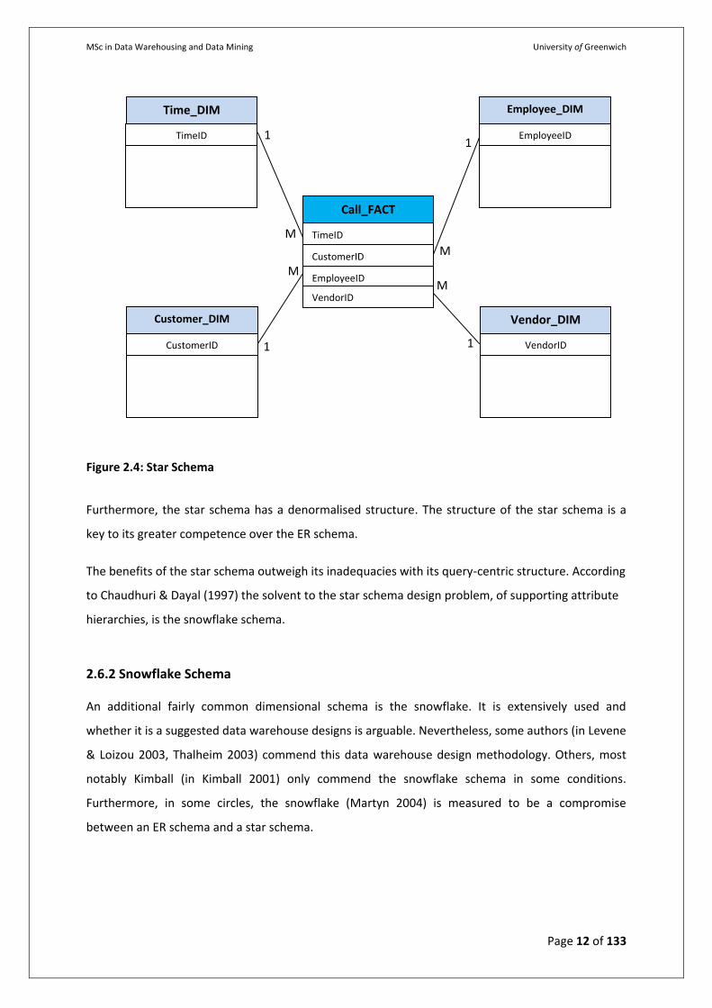
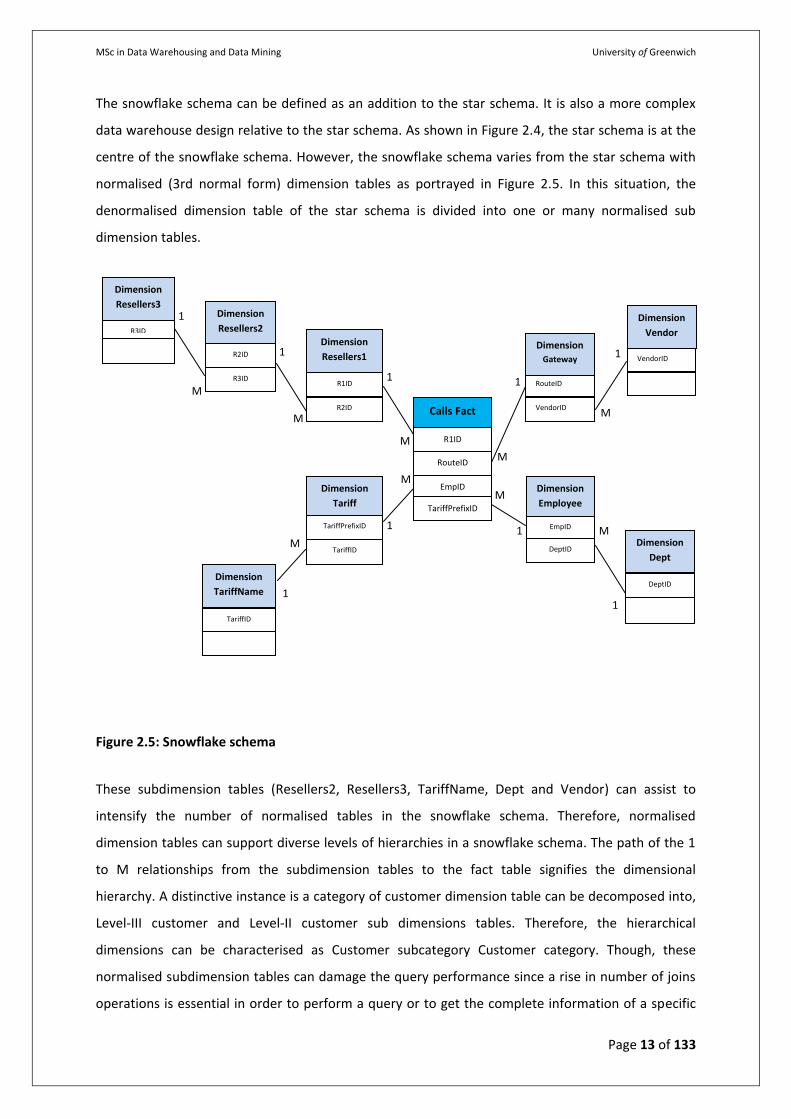
The snowflake schema can be defined as an addition to the star schema. It is also a more complex
data warehouse design relative to the star schema. As shown in Figure 2.4, the star schema is at the
centre of the snowflake schema. However, the snowflake schema varies from the star schema with
normalised (3rd normal form) dimension tables as portrayed in Figure 2.5. In this situation, the
denormalised dimension table of the star schema is divided into one or many normalised sub
dimension tables.
Figure 2.5: Snowflake schema
These subdimension tables (Resellers2, Resellers3, TariffName, Dept and Vendor) can assist to
intensify the number of normalised tables in the snowflake schema. Therefore, normalised
dimension tables can support diverse levels of hierarchies in a snowflake schema. The path of the 1
to M relationships from the subdimension tables to the fact table signifies the dimensional
hierarchy. A distinctive instance is a category of customer dimension table can be decomposed into,
Level-III customer and Level-II customer sub dimensions tables. Therefore, the hierarchical
dimensions can be characterised as Customer subcategory Customer category. Though, these
normalised subdimension tables can damage the query performance since a rise in number of joins
operations is essential in order to perform a query or to get the complete information of a specific
1
M
1
M
1
1 R1ID
Dimension
Resellers1 R2ID
Dimension
Resellers2 R3ID
Dimension
Resellers3
R3ID
R2ID M
1
1 RouteID
Dimension
Gateway VendorID
Dimension
Vendor
1
M 1 EmpID
Dimension
Employee
DeptID
Dimension
Dept
M
M
M
M R1ID
Calls Fact
RouteID
EmpID
TariffPrefixID
1
M
TariffPrefixID
Dimension
Tariff
TariffID
Dimension
TariffName
TariffID DeptID
VendorID
MSc in Data Warehousing and Data Mining University of Greenwich
Page 14 of 133
component. Then again, the subdimension tables in a snowflake can help condense the problems of
data redundancy in denormalised structure of the star schema. The normalisation of the snowflake
schema can also help users view more detail information relative to the star schema (Martyn 2004).
Other advantages that can be extracted from the snowflake schema are: design is easy to
understand as relative to the ER schema; space of aggregate data (Levene & Loizou 2003); easy for
extension by accumulation of new sub dimensions without interfering (Levene & Loizou 2003), data
redundancy is removed through normalised dimension tables, stashes in storage disk space as
relative to the star schema.
Moreover, the disadvantages of the snowflake schema are: decreased query performance as relative
to the star schema because its larger number of joins, huge complexity for the user with increased
number of joins prerequisite for queries. In contrast, it is significant to distinguish that the (IBM
2005) snowflake query performance can meaningfully be better than the star schema if the
dimension tables are very bulky. Likewise, if the dimension tables are big with very large number of
records or wide with large number of attributes then the snowflake schema is suggested (Kimball
2001b, Bhat & Kumar 2000).
The snowflake schema remains a vague topic within the literature as there are a few various
methodologies to normalise dimension tables. Some of these approaches are (Ponniah 2001):
1. Every dimension table are fully normalised.
2. Only a few dimension tables are partially or fully normalised.
3. Every dimension table are partially normalised.
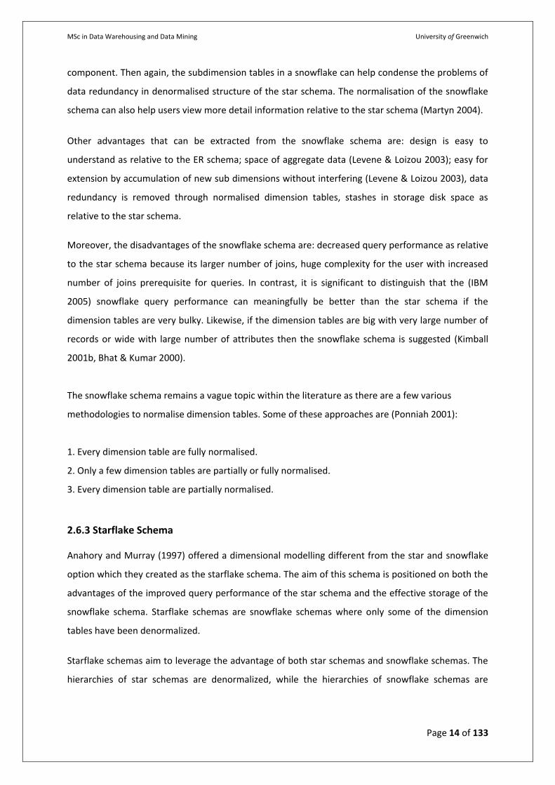
2.6.3 Starflake Schema
Anahory and Murray (1997) offered a dimensional modelling different from the star and snowflake
option which they created as the starflake schema. The aim of this schema is positioned on both the
advantages of the improved query performance of the star schema and the effective storage of the
snowflake schema. Starflake schemas are snowflake schemas where only some of the dimension
tables have been denormalized.
Starflake schemas aim to leverage the advantage of both star schemas and snowflake schemas. The
hierarchies of star schemas are denormalized, while the hierarchies of snowflake schemas are
MSc in Data Warehousing and Data Mining University of Greenwich
Page 15 of 133
normalized. Starflake schemas are normalized to eliminate any redundancies in the dimensions. To
normalize the schema, the shared dimensional hierarchies are placed in outriggers.
[IBM (n,d)]
Figure 2.6: Starflake schema with one fact and two dimensions that share an outrigger.
2.7 OLAP Architecture
The key implementation of the data warehouse is OLAP technology. OLAP is another argumentative
research topic which is talked in this exploration study. OLAP technology is important with the
intention of performing dimensional data analysis tasks from information within a data warehouse.
There is still an argument, within the research community and OLAP vendors, about the favoured
OLAP type essential in order to support OLAP tasks. The three key OLAP categories are:
Multidimensional OLAP (MOLAP), Relational OLAP (ROLAP) and Hybrid OLAP (HOLAP).
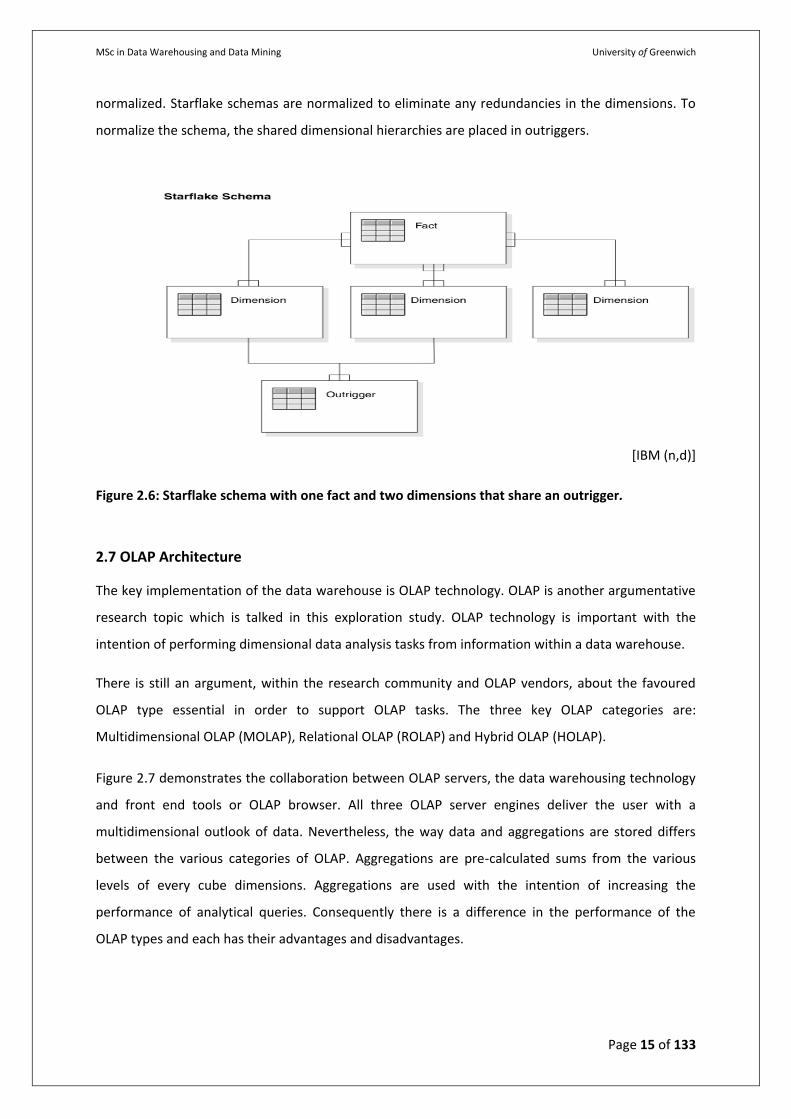
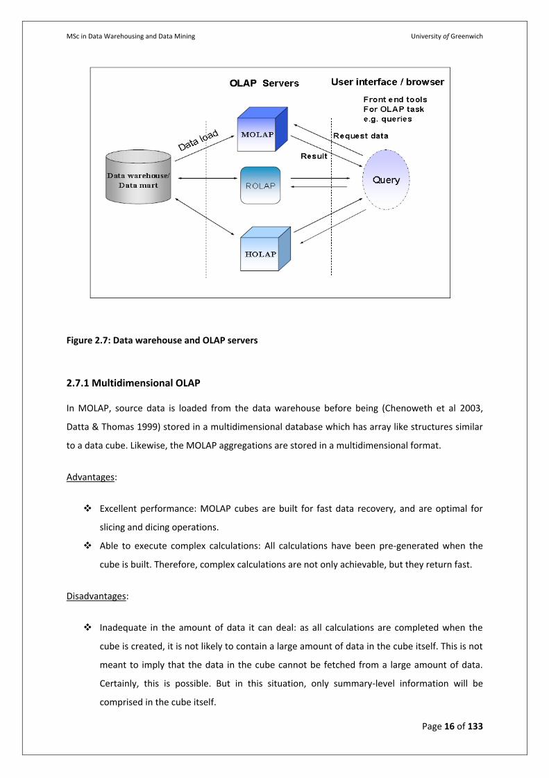
Figure 2.7 demonstrates the collaboration between OLAP servers, the data warehousing technology
and front end tools or OLAP browser. All three OLAP server engines deliver the user with a
multidimensional outlook of data. Nevertheless, the way data and aggregations are stored differs
between the various categories of OLAP. Aggregations are pre-calculated sums from the various
levels of every cube dimensions. Aggregations are used with the intention of increasing the
performance of analytical queries. Consequently there is a difference in the performance of the
OLAP types and each has their advantages and disadvantages.
MSc in Data Warehousing and Data Mining University of Greenwich
Page 16 of 133
Figure 2.7: Data warehouse and OLAP servers
2.7.1 Multidimensional OLAP
In MOLAP, source data is loaded from the data warehouse before being (Chenoweth et al 2003,
Datta & Thomas 1999) stored in a multidimensional database which has array like structures similar
to a data cube. Likewise, the MOLAP aggregations are stored in a multidimensional format.
Advantages:
Excellent performance: MOLAP cubes are built for fast data recovery, and are optimal for
slicing and dicing operations.
Able to execute complex calculations: All calculations have been pre-generated when the
cube is built. Therefore, complex calculations are not only achievable, but they return fast.
Disadvantages:
Inadequate in the amount of data it can deal: as all calculations are completed when the
cube is created, it is not likely to contain a large amount of data in the cube itself. This is not
meant to imply that the data in the cube cannot be fetched from a large amount of data.
Certainly, this is possible. But in this situation, only summary-level information will be
comprised in the cube itself.
MSc in Data Warehousing and Data Mining University of Greenwich
Page 17 of 133
Necessitates additional investment: Cube technology is often exclusive and does not already
exist in the organization. For that reason, to adopt MOLAP technology, chances are
additional investments in human and capital resources are necessary.
2.7.2 Relational OLAP
In ROLAP, data is stored in a relational database, as a set of dimension tables and fact tables, alike a
star or snowflake structure (Chenoweth et al 2003, Datta & Thomas 1999, Vassiliadis & Sellis 1999)
correspondingly, ROLAP aggregations are stored in relational tables within the source.
2.7.3 Hybrid OLAP
HOLAP is a hybrid technology which mixes both MOLAP and ROLAP features. Therefore, both kind of
storage used by MOLAP and ROLAP are used by HOLAP. As a result, HOLAP stores its aggregations in
a multi-dimensional format same as MOLAP. Then again, its data storage is similar to ROLAP. It also
brings the benefits of both MOLAP and ROLAP together. Therefore, it has the quick query
performance of MOLAP and storage effectiveness of ROLAP. Nevertheless, according to research
carried out by Kaser and Lemire (2005) HOLAP has an even a better storage effectiveness relative to
ROLAP.
2.8 ETL role in Data Warehousing and reporting
ETL is for Extract, Transform and Load process of database. This process acts the most significant
part in data warehouse and BI project development since it’s satisfying the analytical obligation of
the project. Data that comes for the reporting is managed by the ETL. Performance, scheduling and
precision of reports are also depends on the ETL processing. Nowadays businesses are integrating
because of the present high competitive market and because of these businesses if businesses want
to implement the BI reporting systems then they also need to join their databases. At this phase ETL
plays vital role for integration of the databases.
The second most significant phase of the ETL method is the data conversion or data cleaning. Only
quality or cleaned data can deliver the superiority decisions or we can say it is the basis of all the
business intelligence actions in the business. Inadequate and imprecise data are not convincing and
cost effective for the business because inadequate or unclean data offers false inference and
erroneous decisions at many levels of the business actions. Dirty data is also threat to the everyday
practice of the business and lead the business to the incorrect track. The goal of data cleansing is to
develop the data superiority and enhance the ETL procedure. In this procedure it eliminates the
wrong, unreliable, duplicate and improperly formatted data before loading it to the data warehouse.
MSc in Data Warehousing and Data Mining University of Greenwich
Page 18 of 133
By removing, moving or by adding the precise data this process leads to the successful BI reporting
system creation. The efficiency of data operational procedure is significantly increased by data
cleansing procedure. Without data cleansing it guides the business to the unsuccessful work
presentation and increases the difficulties in the future. And in the last load procedure the ETL
conveys the data to the data warehouse. Therefore, generally we can say the ETL procedure has a
vital role in the BI reporting.
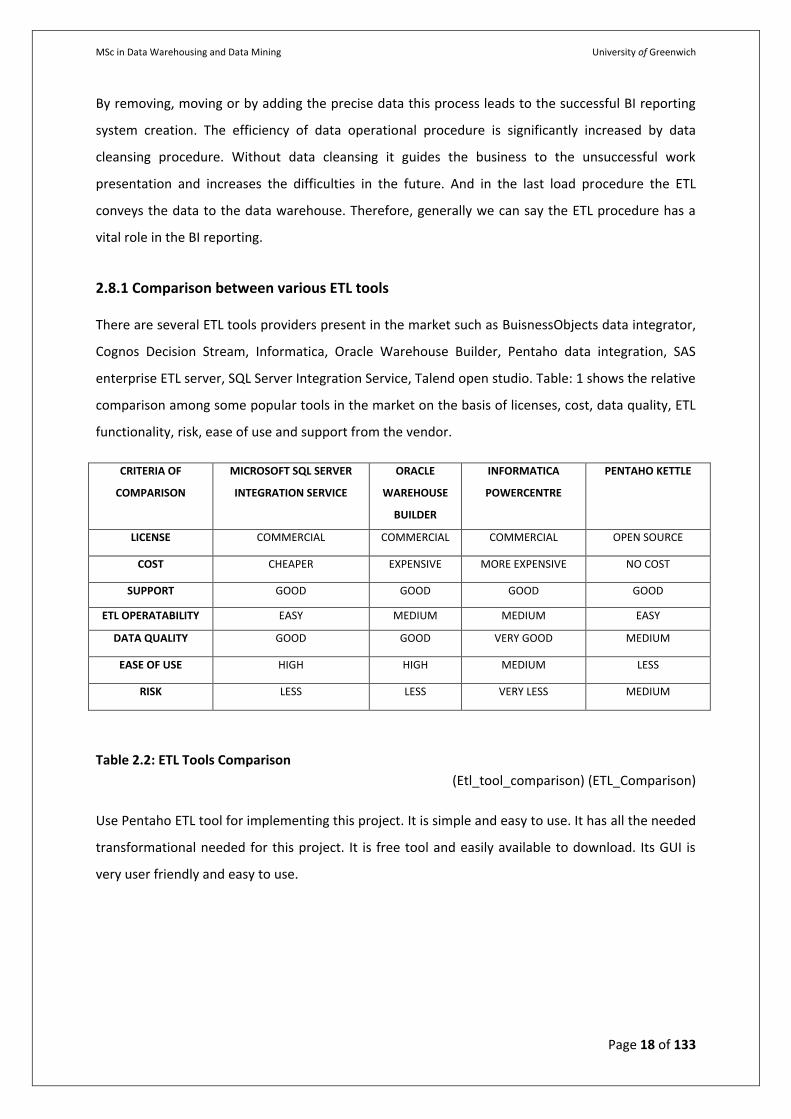
2.8.1 Comparison between various ETL tools
There are several ETL tools providers present in the market such as BuisnessObjects data integrator,
Cognos Decision Stream, Informatica, Oracle Warehouse Builder, Pentaho data integration, SAS
enterprise ETL server, SQL Server Integration Service, Talend open studio. Table: 1 shows the relative
comparison among some popular tools in the market on the basis of licenses, cost, data quality, ETL
functionality, risk, ease of use and support from the vendor.
CRITERIA OF
COMPARISON
MICROSOFT SQL SERVER
INTEGRATION SERVICE
ORACLE
WAREHOUSE
BUILDER
INFORMATICA
POWERCENTRE
PENTAHO KETTLE
LICENSE COMMERCIAL COMMERCIAL COMMERCIAL OPEN SOURCE
COST CHEAPER EXPENSIVE MORE EXPENSIVE NO COST
SUPPORT GOOD GOOD GOOD GOOD
ETL OPERATABILITY EASY MEDIUM MEDIUM EASY
DATA QUALITY GOOD GOOD VERY GOOD MEDIUM
EASE OF USE HIGH HIGH MEDIUM LESS
RISK LESS LESS VERY LESS MEDIUM
Table 2.2: ETL Tools Comparison
(Etl_tool_comparison) (ETL_Comparison)
Use Pentaho ETL tool for implementing this project. It is simple and easy to use. It has all the needed
transformational needed for this project. It is free tool and easily available to download. Its GUI is
very user friendly and easy to use.
MSc in Data Warehousing and Data Mining University of Greenwich
Page 19 of 133
2.8.2 Pentaho Kettle ETL Tools
Data is universal. Providing a steady, distinct version of the reality through all origins of information
is one of the major challenges confronted by IT organizations today. Pentaho Data Integration
provides with great Extraction, Transformation and Loading (ETL) abilities with an innovative,
metadata-driven method. The simplicity of use in our graphical, drag-and-drop design enhances
productivity and our extensible; standards based architecture makes sure that one will never be
required to embrace proprietary methodologies into your ETL solution.
2.8.2.1 Enterprise-Class ETL
Broad out-of-the-box data source support with rushed applications, many open source and
registered database platforms, flat files, Excel documents
Repository-based distributing easy re-use of transformation mechanisms, multi-developer
cooperation, and organized management of models, connections, logs and so on
Pentaho Data Integration (n.d.)
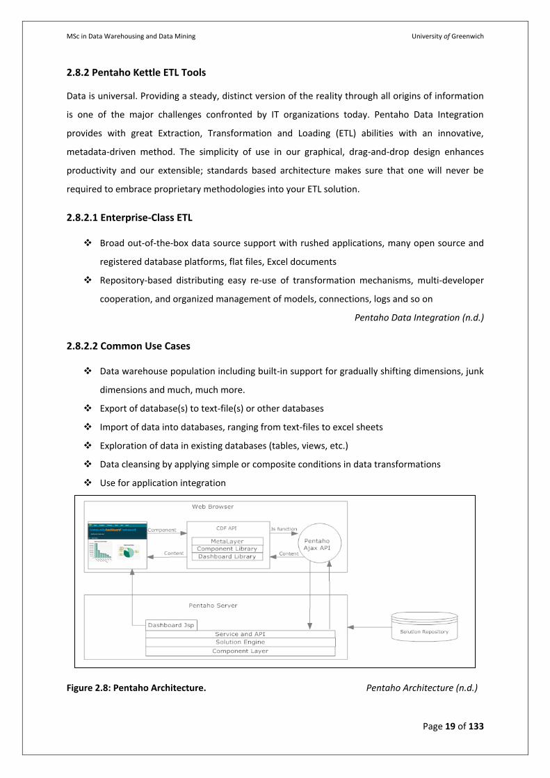
2.8.2.2 Common Use Cases
Data warehouse population including built-in support for gradually shifting dimensions, junk
dimensions and much, much more.
Export of database(s) to text-file(s) or other databases
Import of data into databases, ranging from text-files to excel sheets
Exploration of data in existing databases (tables, views, etc.)
Data cleansing by applying simple or composite conditions in data transformations
Use for application integration
Figure 2.8: Pentaho Architecture. Pentaho Architecture (n.d.)
MSc in Data Warehousing and Data Mining University of Greenwich
Page 20 of 133
2.9 Data Visualization
Data visualization is the study of the visual representation of data, which is "information that has
been abstracted in some schematic form, including attributes or variables for the units of
information".
The most often used data visualization methods is bar chart, pie chart and line chart techniques.
With the change of technology various graphical indicators, impressive and interactive visualization
techniques, applications and dashboards for data visualization are offered in the market. Using these
graphical indicator users can see the point scale value of the graphs and interactive dashboard
allows user to view data in the three dimensional forms. Therefore we can say choice of an
appropriate data visualization method is essential for the any business intelligence reporting system.
(DAVID ADAMS, ACCENTURE)
According to Friedman (2008) the important objective of data visualization is conforming
information clearly and competently through visual means. It doesn’t mean that data visualization
necessitates a dull look to be functional or extremely intricate to have a handsome look. To converse
ideas proficiently, both aesthetical form and functional requirement go hand in hand, letting for
understandings into a further sparse and complex data set by intercommunicating its vital-aspects in
a more impulsive way. Nevertheless, designers repeatedly fail to accomplish equilibrium between
design and function, generating attractive data visualizations which fail to encounter their chief
purpose — to communicate information". In fact, Fernanda Viegas and Martin M. Wattenberg have
acclaimed that a faultless visualization should not just communicate clearly, but stimulate observer
participation and devotion.
Data visualization is intensely associated to information graphics, information visualization, scientific
visualization and statistical graphics. In the new millennium data visualization has transformed into a
dynamic topic of research, study and development. According to Post et al. (2002) it has united the
region of scientific and information visualization".
MSc in Data Warehousing and Data Mining University of Greenwich
Page 21 of 133
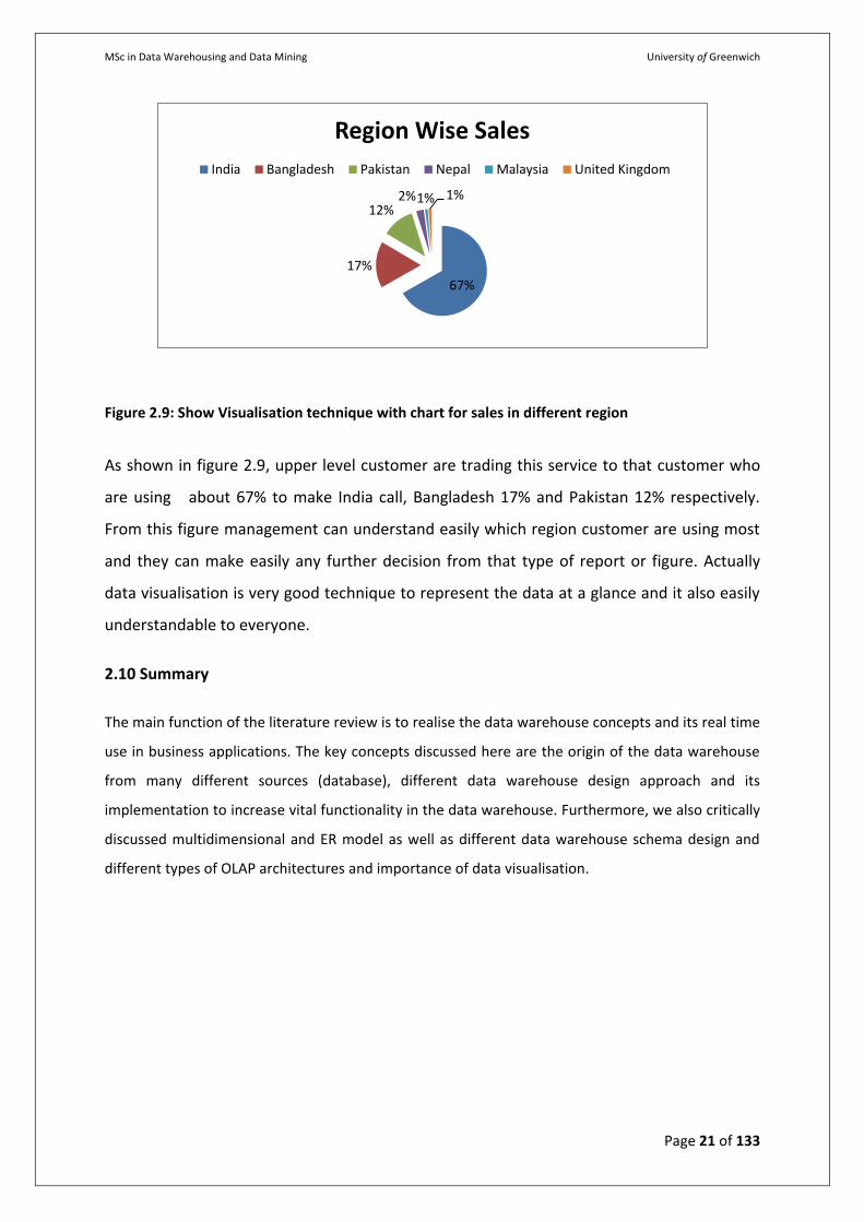
Figure 2.9: Show Visualisation technique with chart for sales in different region
As shown in figure 2.9, upper level customer are trading this service to that customer who
are using about 67% to make India call, Bangladesh 17% and Pakistan 12% respectively.
From this figure management can understand easily which region customer are using most
and they can make easily any further decision from that type of report or figure. Actually
data visualisation is very good technique to represent the data at a glance and it also easily
understandable to everyone.
2.10 Summary
The main function of the literature review is to realise the data warehouse concepts and its real time
use in business applications. The key concepts discussed here are the origin of the data warehouse
from many different sources (database), different data warehouse design approach and its
implementation to increase vital functionality in the data warehouse. Furthermore, we also critically
discussed multidimensional and ER model as well as different data warehouse schema design and
different types of OLAP architectures and importance of data visualisation.
67%
17%
12% 2% 1% 1%
Region Wise Sales
India Bangladesh Pakistan Nepal Malaysia United Kingdom
MSc in Data Warehousing and Data Mining University of Greenwich
Page 22 of 133
Chapter 3
Requirement analysis and design
3.1 Overview
“Software requirement analysis is the documentation, analysis and specification of common
necessity from a specific application domain”. (PRESSMAN, Roger S, 2004) This chapter describes the
present existing system of the organization that shows the requirement of this project. This chapter
comprises design of the current system and design of the data warehouse. At the end of this chapter
the architecture of the proposed BI reporting system is explained.
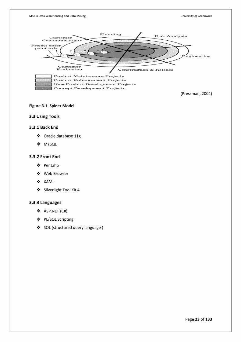
3.2 Software Process Model
Software process model is the combination of the software design, development, testing and
customer evaluation stages. There are different software process models like LINEAR SEQUNTIAL
MODEL, RAD MODEL, PROTOTYPING MODEL, INCREMENTAL MODEL and SPIRAL MODEL. For
software like business intelligence reporting system customer evaluation and planning are the most
important stages and requires to evaluation at every stages of the development by bearing in mind
that spiral model is the best fit for this software development process specially to implement BI
report with ASP.NET with Silverlight.
The aim of customer communication is to form operational communication between
developer and customer. The planning objectives are to outline resources, project
alternatives, time lines and other project associated information. The drive of the risk
analysis stage is to measure both technical and management risks. The engineering task is
to build one or more demonstrations of the application. The construction and release task –
to build, test, install and offer user. The customer evaluation task - to obtain customer
feedback on the basis of evaluation of the software representation generated during the
engineering phase and applied during the install phase. [Sprial Lifecycle Model (n.d.)]
MSc in Data Warehousing and Data Mining University of Greenwich
Page 23 of 133
(Pressman, 2004)
Figure 3.1. Spider Model
3.3 Using Tools
3.3.1 Back End
Oracle database 11g
MYSQL
3.3.2 Front End
Pentaho
Web Browser
XAML
Silverlight Tool Kit 4
3.3.3 Languages
ASP.NET (C#)
PL/SQL Scripting
SQL (structured query language )
MSc in Data Warehousing and Data Mining University of Greenwich
Page 24 of 133
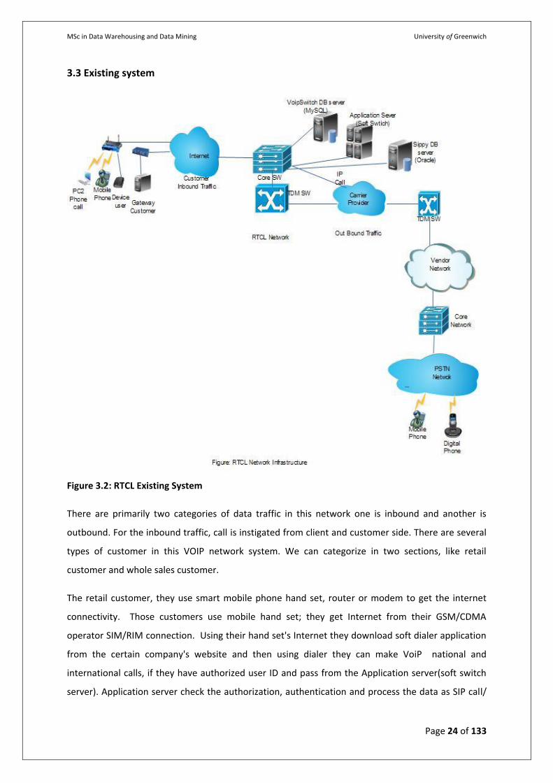
3.3 Existing system
Figure 3.2: RTCL Existing System
There are primarily two categories of data traffic in this network one is inbound and another is
outbound. For the inbound traffic, call is instigated from client and customer side. There are several
types of customer in this VOIP network system. We can categorize in two sections, like retail
customer and whole sales customer.
The retail customer, they use smart mobile phone hand set, router or modem to get the internet
connectivity. Those customers use mobile hand set; they get Internet from their GSM/CDMA
operator SIM/RIM connection. Using their hand set's Internet they download soft dialer application
from the certain company's website and then using dialer they can make VoiP national and
international calls, if they have authorized user ID and pass from the Application server(soft switch
server). Application server check the authorization, authentication and process the data as SIP call/
MSc in Data Warehousing and Data Mining University of Greenwich
Page 25 of 133
VoiP call, if the billing server responses that particular customer has sufficient balance to retrieve
information for database to make the call then call routed to the vendors networks, if the call is TDM
call then application server send it to the RTCL TDM switch then TDM switch sends the call to the
vendor network. Otherwise call will pass as an IP call to then vendor networks. In the above picture
mention customer also as a retail customer.
From the vendors network VoIP call process and terminated to the PSTN operator network and then
PSTN network connect to the desire destination phone or mobile Number.
Another most important customer type is Gateway customer who is treating the whole sales
customer. They have own VoIP retail customer which are processing with the billing server and
database server. In this case RTCL working like vendor to them. For whole sales customers are
handling with Sippy Soft (and Oracle billing server of RTCL) then rest of process is similar to retails
customer.
So, Raiyan Telecom/Carrier Ltd (RTCL) are using two billing System. One DB (VOIPSWITCH) is for
retail customers, which is not capable to handle high volume of parallel calls but it is very easy to
operate for customers who have not much technical knowledge. On the other hand, another billing
system is using for whole sales customers which can handle high volume of parallel calls but not easy
to operate for customer. These two Database Servers are located at the same location in London,
UK. They used the different database management system. For Voipswitch billing system RTCL is
using the MYSQL database management system and for Sippy billing system it is using the Oracle
database management system. In the current situation Management using different billing reporting
system and they manually do summation with Excel to find out the current sales and usages and
situation of the company and extract that queries results into the Microsoft excel and use that excel
sheets for the decision making which is very time consuming task.
Entity relationship diagram for the both database management system are given below.
MSc in Data Warehousing and Data Mining University of Greenwich
Page 26 of 133
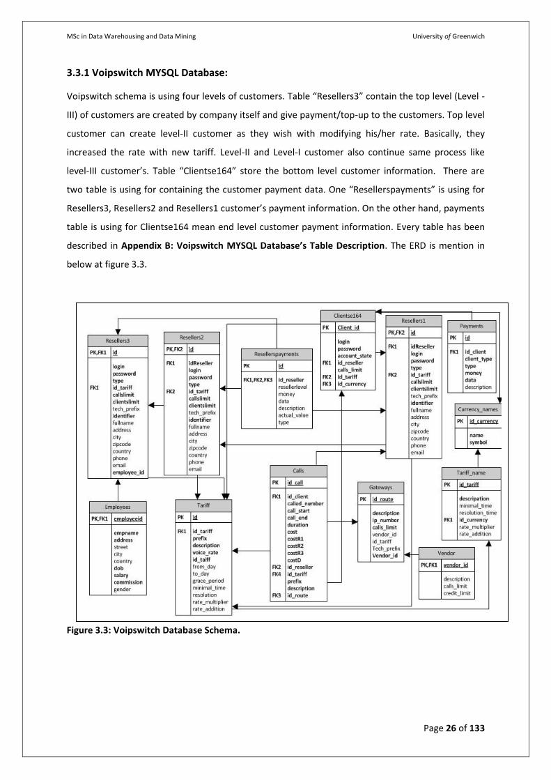
3.3.1 Voipswitch MYSQL Database:
Voipswitch schema is using four levels of customers. Table “Resellers3” contain the top level (Level -
III) of customers are created by company itself and give payment/top-up to the customers. Top level
customer can create level-II customer as they wish with modifying his/her rate. Basically, they
increased the rate with new tariff. Level-II and Level-I customer also continue same process like
level-III customer’s. Table “Clientse164” store the bottom level customer information. There are
two table is using for containing the customer payment data. One “Resellerspayments” is using for
Resellers3, Resellers2 and Resellers1 customer’s payment information. On the other hand, payments
table is using for Clientse164 mean end level customer payment information. Every table has been
described in Appendix B: Voipswitch MYSQL Database’s Table Description. The ERD is mention in
below at figure 3.3.
Figure 3.3: Voipswitch Database Schema.
MSc in Data Warehousing and Data Mining University of Greenwich
Page 27 of 133
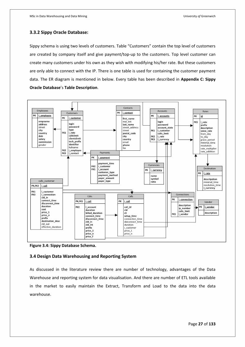
3.3.2 Sippy Oracle Database:
Sippy schema is using two levels of customers. Table “Customers” contain the top level of customers
are created by company itself and give payment/top-up to the customers. Top level customer can
create many customers under his own as they wish with modifying his/her rate. But these customers
are only able to connect with the IP. There is one table is used for containing the customer payment
data. The ER diagram is mentioned in below. Every table has been described in Appendix C: Sippy
Oracle Database’s Table Description.
Figure 2: Sippy Database Schema.
As mentioned on the Figure 1 and 2 a database diagram of both RTCL’s schemas is using the
different schema in the both database management system.
Figure 3.4: Sippy Database Schema.
3.4 Design Data Warehousing and Reporting System
As discussed in the literature review there are number of technology, advantages of the Data
Warehouse and reporting system for data visualisation. And there are number of ETL tools available
in the market to easily maintain the Extract, Transform and Load to the data into the data
warehouse.
MSc in Data Warehousing and Data Mining University of Greenwich
Page 28 of 133
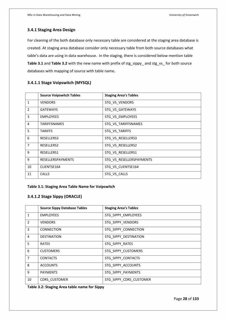
3.4.1 Staging Area Design
For cleaning of the both database only necessary table are considered at the staging area database is
created. At staging area database consider only necessary table from both source databases what
table’s data are using in data warehouse. In the staging, there is considered below mention table
Table 3.1 and Table 3.2 with the new name with prefix of stg_sippy_ and stg_vs_ for both source
databases with mapping of source with table name.
3.4.1.1 Stage Voipswitch (MYSQL)
Source Voipswitch Tables Staging Area’s Tables
1 VENDORS STG_VS_VENDORS
2 GATEWAYS STG_VS_GATEWAYS
3 EMPLOYEES STG_VS_EMPLOYEES
4 TARIFFSNAMES STG_VS_TARIFFSNAMES
5 TARIFFS STG_VS_TARIFFS
6 RESELLERS3 STG_VS_RESELLERS3
7 RESELLERS2 STG_VS_RESELLERS2
9 RESELLERS1 STG_VS_RESELLERS1
9 RESELLERSPAYMENTS STG_VS_RESELLERSPAYMENTS
10 CLIENTSE164 STG_VS_CLIENTSE164
11 CALLS STG_VS_CALLS
Table 3.1: Staging Area Table Name for Voipswitch
3.4.1.2 Stage Sippy (ORACLE)
Source Sippy Database Tables Staging Area’s Tables
1 EMPLOYEES STG_SIPPY_EMPLOYEES
2 VENDORS STG_SIPPY_VENDORS
3 CONNECTION STG_SIPPY_CONNECTION
4 DESTINATION STG_SIPPY_DESTINATION
5 RATES STG_SIPPY_RATES
6 CUSTOMERS STG_SIPPY_CUSTOMERS
7 CONTACTS STG_SIPPY_CONTACTS
8 ACCOUNTS STG_SIPPY_ACCOUNTS
9 PAYMENTS STG_SIPPY_PAYMENTS
10 CDRS_CUSTOMER STG_SIPPY_CDRS_CUSTOMER
Table 3.2: Staging Area table name for Sippy
MSc in Data Warehousing and Data Mining University of Greenwich
Page 29 of 133
3.4.2 Data warehouse design decisions
Design of the data warehouse has a vital role for optimization of the data warehouse query writing.
There are essentially two kinds of design decisions for data warehouse schema design: star schema
and snowflake schema. Of these two schemas, star schema is very frequently used for the schema
design. In the star schema inadequate number of joins is created to execute report queries which
are very useful for the query optimization. With existing data source it is suitable to star schema.
The figure below shows the star schema design of the system data warehouse. As seen in the Figure
3.5 design it appears that there are five dimensions and two fact tables.
Each end of the star in the figure below represents the five dimension table and two fact tables. One
fact table Call_FACT contains the proposed measure of the data warehouse like call duration, per call
cost amount for customer and the foreign keys form the dimension table (Time_DIM,
Employee_DIM, Customer_DIM, Vendor_DIM and Location_DIM). Call_Fact table contains also
serverid to identified sales or usages for particular billing system or Server to differentiate type of
customers like whole sales customer or retails. Another Fact Payment_FACT table contains the top-
up amount to the customer and foreign keys from the dimension table (Time_DIM, Employee_DIM
and Customer_DIM). Previous section discusses about the level of customer for each data source.
For designing data warehousing do not need to every level of customer. So, In the Voipswitch data
source, only consider the Top level of customer (Resellers3) information because Resellers3
customer only dealing with the company and also consider resellerspayments table information and
select only the Reseller Level-3 customer top-up information. So, Resellers2 and Resellers1 and
Clinetse164 are not considering in design to Data Warehousing implementation. For Sippy data
source, only consider the Customer table information but not Account table’s customer (low level of
customer) information. This is because, top level of customer information dealing with RTCL whom
information contain the “Customer” Table and for these customer top-up or payment information
only consider customer related payment information and ignore the accounts related payment
information. Time Dimension table is generated using the procedure for particular dates. In vendor
and employee dimension contains the basic information of vendor and employees. All Dimension
and Face table are crated on the basis of tables shown in Appendix D: Dimension and FACT Table
Analysis.
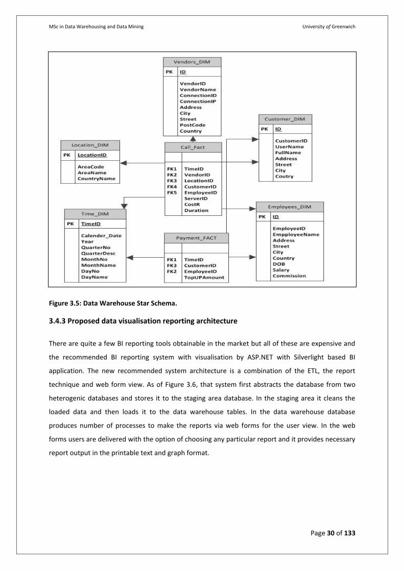
MSc in Data Warehousing and Data Mining University of Greenwich
Page 30 of 133
Figure 3.5: Data Warehouse Star Schema.
3.4.3 Proposed data visualisation reporting architecture
There are quite a few BI reporting tools obtainable in the market but all of these are expensive and
the recommended BI reporting system with visualisation by ASP.NET with Silverlight based BI
application. The new recommended system architecture is a combination of the ETL, the report
technique and web form view. As of Figure 3.6, that system first abstracts the database from two
heterogenic databases and stores it to the staging area database. In the staging area it cleans the
loaded data and then loads it to the data warehouse tables. In the data warehouse database
produces number of processes to make the reports via web forms for the user view. In the web
forms users are delivered with the option of choosing any particular report and it provides necessary
report output in the printable text and graph format.
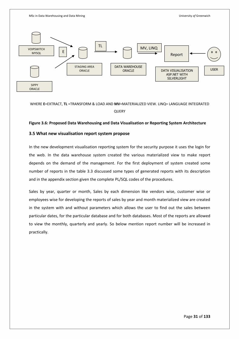
MSc in Data Warehousing and Data Mining University of Greenwich
Page 31 of 133
WHERE E=EXTRACT, TL =TRANSFORM & LOAD AND MV=MATERIALIZED VIEW. LINQ= LANGUAGE INTEGRATED
QUERY
Figure 3.6: Proposed Data Warehousing and Data Visualisation or Reporting System Architecture
3.5 What new visualisation report system propose
In the new development visualisation reporting system for the security purpose it uses the login for
the web. In the data warehouse system created the various materialized view to make report
depends on the demand of the management. For the first deployment of system created some
number of reports in the table 3.3 discussed some types of generated reports with its description
and in the appendix section given the complete PL/SQL codes of the procedures.
Sales by year, quarter or month, Sales by each dimension like vendors wise, customer wise or
employees wise for developing the reports of sales by year and month materialized view are created
in the system with and without parameters which allows the user to find out the sales between
particular dates, for the particular database and for both databases. Most of the reports are allowed
to view the monthly, quarterly and yearly. So below mention report number will be increased in
practically.
TL
E MV, LINQ VOIPSWITCH
MYSQL
SIPPY ORACLE
STAGING AREA ORACLE
DATA WAREHOUSE ORACLE
QLSERVER
Report
DATA VISUALISATION ASP.NET WITH SILVERLIGHT
MS
MS SQL SERVER
USER
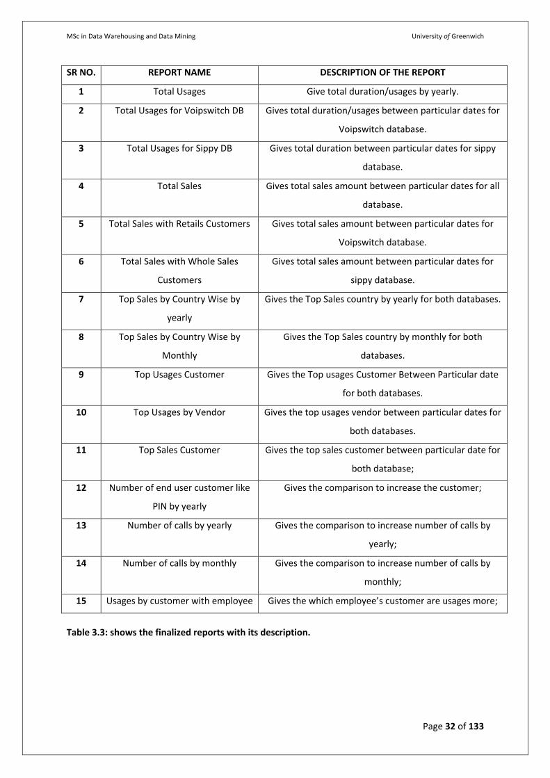
MSc in Data Warehousing and Data Mining University of Greenwich
Page 32 of 133
SR NO. REPORT NAME DESCRIPTION OF THE REPORT
1 Total Usages Give total duration/usages by yearly.
2 Total Usages for Voipswitch DB Gives total duration/usages between particular dates for
Voipswitch database.
3 Total Usages for Sippy DB Gives total duration between particular dates for sippy
database.
4 Total Sales Gives total sales amount between particular dates for all
database.
5 Total Sales with Retails Customers Gives total sales amount between particular dates for
Voipswitch database.
6 Total Sales with Whole Sales
Customers
Gives total sales amount between particular dates for
sippy database.
7 Top Sales by Country Wise by
yearly
Gives the Top Sales country by yearly for both databases.
8 Top Sales by Country Wise by
Monthly
Gives the Top Sales country by monthly for both
databases.
9 Top Usages Customer Gives the Top usages Customer Between Particular date
for both databases.
10 Top Usages by Vendor Gives the top usages vendor between particular dates for
both databases.
11 Top Sales Customer Gives the top sales customer between particular date for
both database;
12 Number of end user customer like
PIN by yearly
Gives the comparison to increase the customer;
13 Number of calls by yearly Gives the comparison to increase number of calls by
yearly;
14 Number of calls by monthly Gives the comparison to increase number of calls by
monthly;
15 Usages by customer with employee Gives the which employee’s customer are usages more;
Table 3.3: shows the finalized reports with its description.
MSc in Data Warehousing and Data Mining University of Greenwich
Page 33 of 133
Chapter 4
Implement Data Warehouse
4.1 Overview
This chapter discusses the information about the implementation of the system which includes the
technology used for implementation, flow of the development process, Implement Data Warehouse,
ETL In the start of this chapter it gives the explanation of the tools used and implementation of the
data warehouse. In the last of this chapter it explains the Pentaho ETL process.
4.2 Technology used for implementation
As discussed in the literature review there are number of different ETL are available in the market
but to show the capability of SQL programming in this system used the Oracle PL/Sql Store
Procedure with different programming technique like cursor, loop, if-else for cleaning and loading of
the data to data warehouse and also use the open source Pentaho ETL tools. To load the data from
the MYSQL database to Oracle used the Pentaho which is very faster, convenient and easy to user
and management.
4.2.1 ETL Tool – Pentaho
Pentaho is an open source and free tools to do the data integration and data transformation. Which
comprises the number of built in tasks for the data transformation. Pentaho has the capabilities to
extract the data from the any sort of destination like xml files, flat files, and relational database and
load that data into any destination. Pentaho has several built in module for the Extract and Load
data and transforming the data from one format to another. As Pentaho matched in the literature
review with other available market tools its free than others and easy to understand for new
starters. Pentaho also allow using many programming language’s customer script like JaveScript,
PL/SQL Script and so on. In this solution it’s used to abstract data from the MYSQL database and load
it to Oracle with the use in between data conversation node. For accessing and managing the tables
in the database and for the formation Pentaho provide the interface for the developers. It comprises
the number of graphical tools for joining with Table with different database sources.
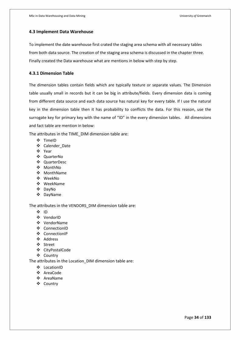
MSc in Data Warehousing and Data Mining University of Greenwich
Page 34 of 133
4.3 Implement Data Warehouse
To implement the date warehouse first crated the staging area schema with all necessary tables
from both data source. The creation of the staging area schema is discussed in the chapter three.
Finally created the Data warehouse what are mentions in below with step by step.
4.3.1 Dimension Table
The dimension tables contain fields which are typically texture or separate values. The Dimension
table usually small in records but it can be big in attribute/fields. Every dimension data is coming
from different data source and each data source has natural key for every table. If I use the natural
key in the dimension table then it has probability to conflicts the data. For this reason, use the
surrogate key for primary key with the name of “ID” in the every dimension tables. All dimensions
and fact table are mention in below:
The attributes in the TIME_DIM dimension table are:
TimeID Calender_Date Year QuarterNo QuarterDesc MonthNo MonthName WeekNo WeekName DayNo DayName
The attributes in the VENDORS_DIM dimension table are:
ID VendorID VendorName ConnectionID ConnectionIP Address Street CityPostalCode Country
The attributes in the Location_DIM dimension table are:
LocationID AreaCode AreaName Country
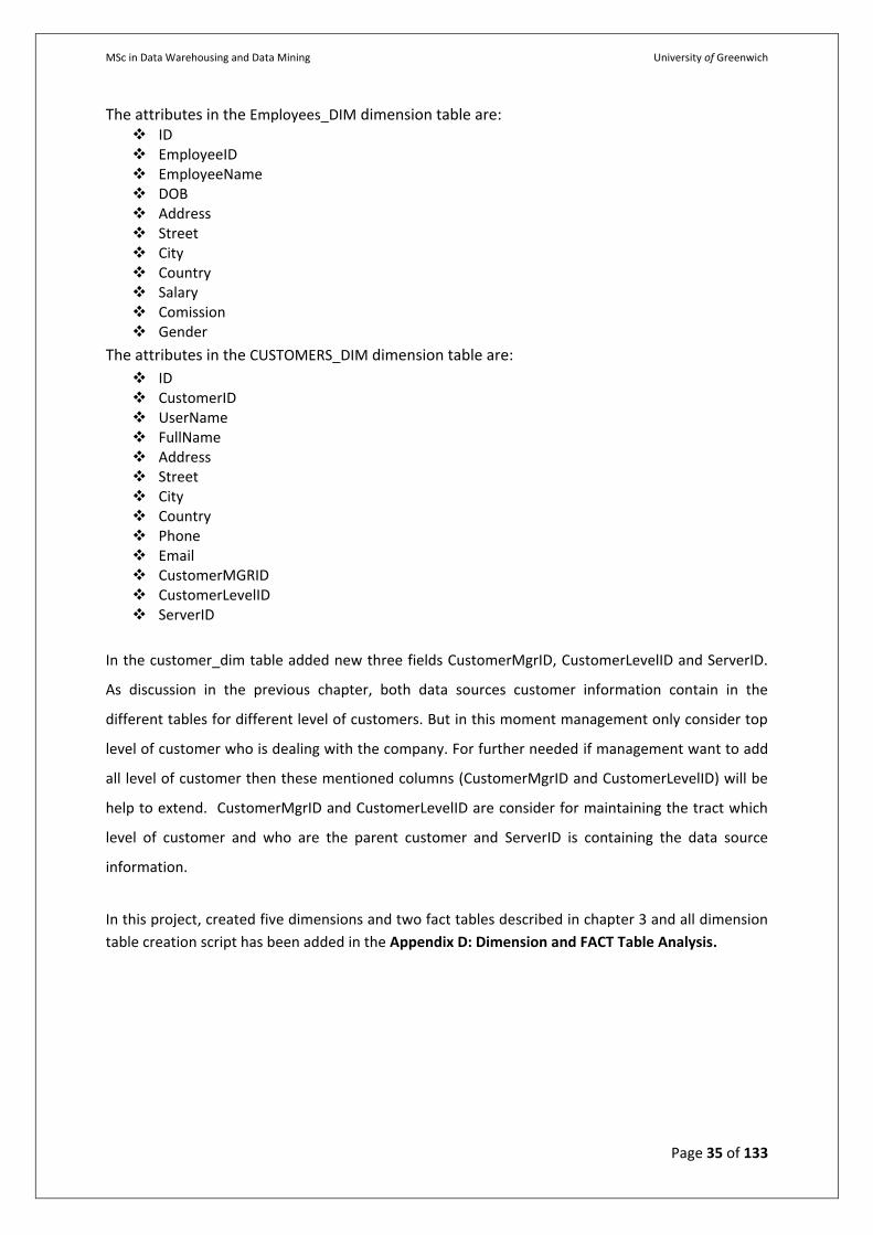
MSc in Data Warehousing and Data Mining University of Greenwich
Page 35 of 133
The attributes in the Employees_DIM dimension table are: ID EmployeeID EmployeeName DOB Address Street City Country Salary Comission Gender
The attributes in the CUSTOMERS_DIM dimension table are:
ID CustomerID UserName FullName Address Street City Country Phone Email CustomerMGRID CustomerLevelID ServerID
In the customer_dim table added new three fields CustomerMgrID, CustomerLevelID and ServerID.
As discussion in the previous chapter, both data sources customer information contain in the
different tables for different level of customers. But in this moment management only consider top
level of customer who is dealing with the company. For further needed if management want to add
all level of customer then these mentioned columns (CustomerMgrID and CustomerLevelID) will be
help to extend. CustomerMgrID and CustomerLevelID are consider for maintaining the tract which
level of customer and who are the parent customer and ServerID is containing the data source
information.
In this project, created five dimensions and two fact tables described in chapter 3 and all dimension
table creation script has been added in the Appendix D: Dimension and FACT Table Analysis.
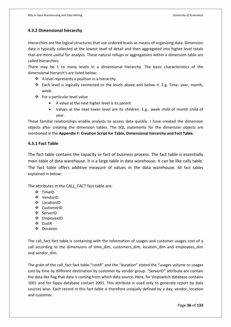
MSc in Data Warehousing and Data Mining University of Greenwich
Page 36 of 133
4.3.2 Dimensional hierarchy
Hierarchies are the logical structures that use ordered levels as means of organizing data. Dimension
data is typically collected at the lowest level of detail and then aggregated into higher level totals
that are more useful for analysis. These natural rollups or aggregations within a dimension table are
called hierarchies.
There may be 1 to many levels in a dimensional hierarchy. The basic characteristics of the
dimensional hierarch’s are listed below:
A level represents a position in a hierarchy
Each level is logically connected to the levels above and below it. E.g. Time: year, month,
week.
For a particular level value
A value at the next higher level is its parent
Values at the next lower level are its children. E.g.: week child of month child of
year.
These familial relationships enable analysts to access data quickly. I have created the dimension
objects after creating the dimension tables. The SQL statements for the dimension objects are
mentioned in the Appendix F: Creation Script for Table, Dimensional hierarchy and Fact Table.
4.3.1 Fact Table
The fact table contains the capacity or fact of business process. The fact table is essentially
main table of data warehouse. It is a large table in data warehouse. It can be like calls table.
The fact table offers additive measure of values in the data warehouse. All fact tables
explained in below:
The attributes in the CALL_FACT fact table are:
TimeID VendorID LocationID CustomerID ServerID EmployeeID CostR Duration
The call_fact fact table is containing with the information of usages and customer usages cost of a
call according to the dimensions of time_dim, customers_dim, location_dim and employees_dim
and vendor_dim.
The grain of the call_fact fact table “costR” and the “duration” stated the “usages volume or usages
cost by time by different destination by customer by vendor group. “ServerID” attribute are contain
the data like flag that data is coming from which data source. Here, for Voipswitch database contains
1001 and for Sippy database contact 2001. This attribute is used only to generate report by data
sources wise. Each record in this fact table is therefore uniquely defined by a day, vendor, location
and customer.
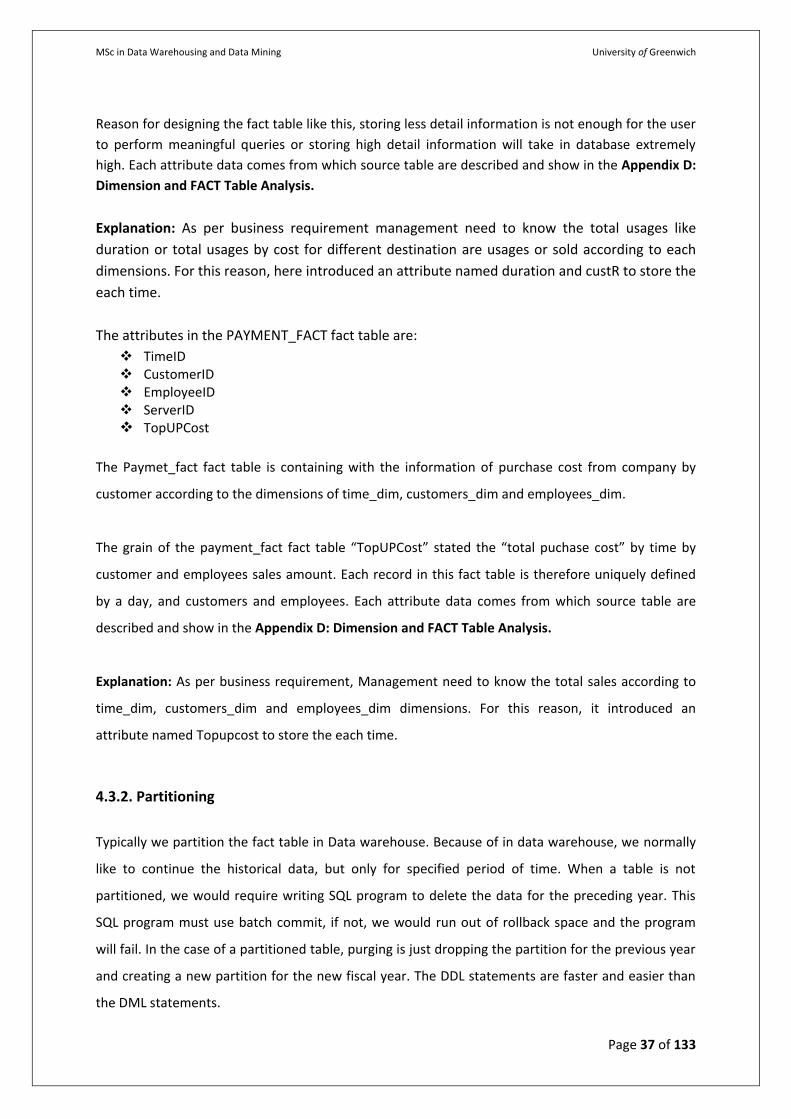
MSc in Data Warehousing and Data Mining University of Greenwich
Page 37 of 133
Reason for designing the fact table like this, storing less detail information is not enough for the user
to perform meaningful queries or storing high detail information will take in database extremely
high. Each attribute data comes from which source table are described and show in the Appendix D:
Dimension and FACT Table Analysis.
Explanation: As per business requirement management need to know the total usages like
duration or total usages by cost for different destination are usages or sold according to each
dimensions. For this reason, here introduced an attribute named duration and custR to store the
each time.
The attributes in the PAYMENT_FACT fact table are:
TimeID CustomerID EmployeeID ServerID TopUPCost
The Paymet_fact fact table is containing with the information of purchase cost from company by
customer according to the dimensions of time_dim, customers_dim and employees_dim.
The grain of the payment_fact fact table “TopUPCost” stated the “total puchase cost” by time by
customer and employees sales amount. Each record in this fact table is therefore uniquely defined
by a day, and customers and employees. Each attribute data comes from which source table are
described and show in the Appendix D: Dimension and FACT Table Analysis.
Explanation: As per business requirement, Management need to know the total sales according to
time_dim, customers_dim and employees_dim dimensions. For this reason, it introduced an
attribute named Topupcost to store the each time.
4.3.2. Partitioning
Typically we partition the fact table in Data warehouse. Because of in data warehouse, we normally
like to continue the historical data, but only for specified period of time. When a table is not
partitioned, we would require writing SQL program to delete the data for the preceding year. This
SQL program must use batch commit, if not, we would run out of rollback space and the program
will fail. In the case of a partitioned table, purging is just dropping the partition for the previous year
and creating a new partition for the new fiscal year. The DDL statements are faster and easier than
the DML statements.
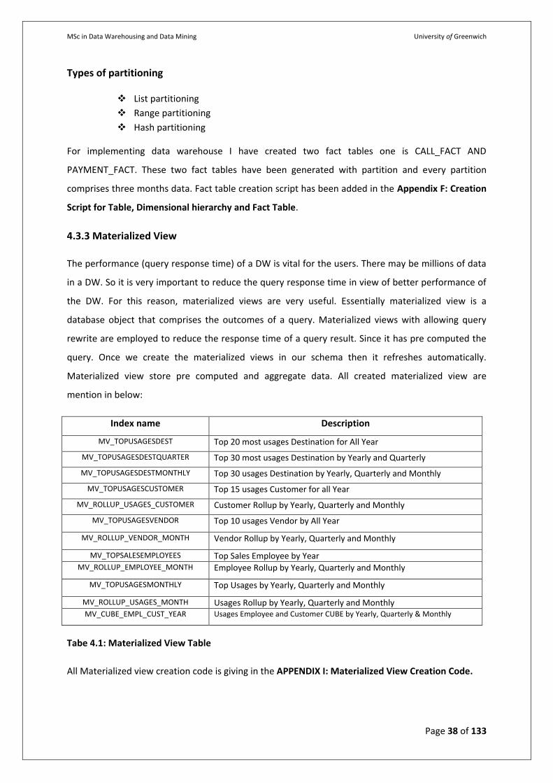
MSc in Data Warehousing and Data Mining University of Greenwich
Page 38 of 133
Types of partitioning
List partitioning
Range partitioning
Hash partitioning
For implementing data warehouse I have created two fact tables one is CALL_FACT AND
PAYMENT_FACT. These two fact tables have been generated with partition and every partition
comprises three months data. Fact table creation script has been added in the Appendix F: Creation
Script for Table, Dimensional hierarchy and Fact Table.
4.3.3 Materialized View
The performance (query response time) of a DW is vital for the users. There may be millions of data
in a DW. So it is very important to reduce the query response time in view of better performance of
the DW. For this reason, materialized views are very useful. Essentially materialized view is a
database object that comprises the outcomes of a query. Materialized views with allowing query
rewrite are employed to reduce the response time of a query result. Since it has pre computed the
query. Once we create the materialized views in our schema then it refreshes automatically.
Materialized view store pre computed and aggregate data. All created materialized view are
mention in below:
Index name Description
MV_TOPUSAGESDEST Top 20 most usages Destination for All Year
MV_TOPUSAGESDESTQUARTER Top 30 most usages Destination by Yearly and Quarterly
MV_TOPUSAGESDESTMONTHLY Top 30 usages Destination by Yearly, Quarterly and Monthly
MV_TOPUSAGESCUSTOMER Top 15 usages Customer for all Year
MV_ROLLUP_USAGES_CUSTOMER Customer Rollup by Yearly, Quarterly and Monthly
MV_TOPUSAGESVENDOR Top 10 usages Vendor by All Year
MV_ROLLUP_VENDOR_MONTH Vendor Rollup by Yearly, Quarterly and Monthly
MV_TOPSALESEMPLOYEES Top Sales Employee by Year MV_ROLLUP_EMPLOYEE_MONTH Employee Rollup by Yearly, Quarterly and Monthly
MV_TOPUSAGESMONTHLY Top Usages by Yearly, Quarterly and Monthly
MV_ROLLUP_USAGES_MONTH Usages Rollup by Yearly, Quarterly and Monthly MV_CUBE_EMPL_CUST_YEAR Usages Employee and Customer CUBE by Yearly, Quarterly & Monthly
Tabe 4.1: Materialized View Table
All Materialized view creation code is giving in the APPENDIX I: Materialized View Creation Code.
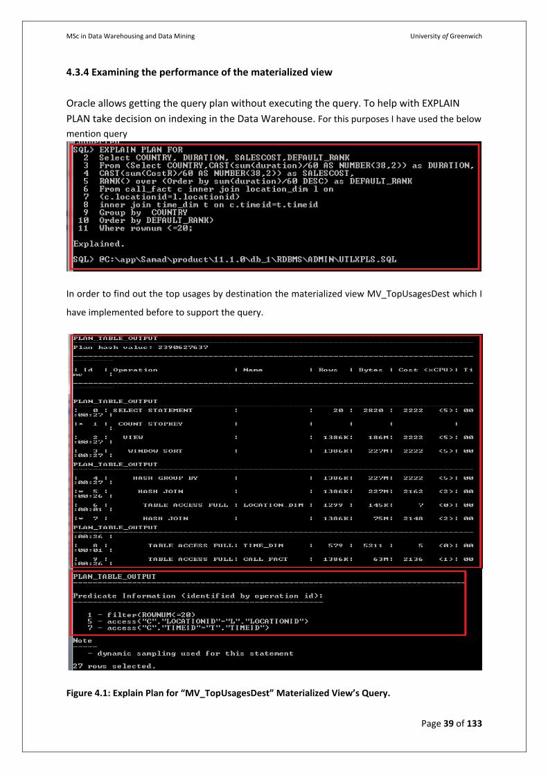
MSc in Data Warehousing and Data Mining University of Greenwich
Page 39 of 133
4.3.4 Examining the performance of the materialized view
Oracle allows getting the query plan without executing the query. To help with EXPLAIN
PLAN take decision on indexing in the Data Warehouse. For this purposes I have used the below
mention query
In order to find out the top usages by destination the materialized view MV_TopUsagesDest which I
have implemented before to support the query.
Figure 4.1: Explain Plan for “MV_TopUsagesDest” Materialized View’s Query.
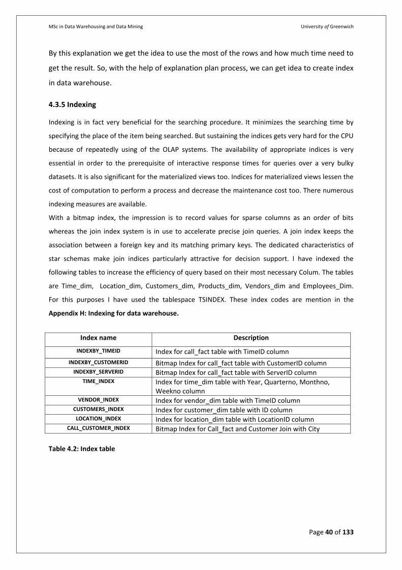
MSc in Data Warehousing and Data Mining University of Greenwich
Page 40 of 133
By this explanation we get the idea to use the most of the rows and how much time need to
get the result. So, with the help of explanation plan process, we can get idea to create index
in data warehouse.
4.3.5 Indexing
Indexing is in fact very beneficial for the searching procedure. It minimizes the searching time by
specifying the place of the item being searched. But sustaining the indices gets very hard for the CPU
because of repeatedly using of the OLAP systems. The availability of appropriate indices is very
essential in order to the prerequisite of interactive response times for queries over a very bulky
datasets. It is also significant for the materialized views too. Indices for materialized views lessen the
cost of computation to perform a process and decrease the maintenance cost too. There numerous
indexing measures are available.
With a bitmap index, the impression is to record values for sparse columns as an order of bits
whereas the join index system is in use to accelerate precise join queries. A join index keeps the
association between a foreign key and its matching primary keys. The dedicated characteristics of
star schemas make join indices particularly attractive for decision support. I have indexed the
following tables to increase the efficiency of query based on their most necessary Colum. The tables
are Time_dim, Location_dim, Customers_dim, Products_dim, Vendors_dim and Employees_Dim.
For this purposes I have used the tablespace TSINDEX. These index codes are mention in the
Appendix H: Indexing for data warehouse.
Index name Description
INDEXBY_TIMEID Index for call_fact table with TimeID column
INDEXBY_CUSTOMERID Bitmap Index for call_fact table with CustomerID column INDEXBY_SERVERID Bitmap Index for call_fact table with ServerID column
TIME_INDEX Index for time_dim table with Year, Quarterno, Monthno, Weekno column
VENDOR_INDEX Index for vendor_dim table with TimeID column CUSTOMERS_INDEX Index for customer_dim table with ID column LOCATION_INDEX Index for location_dim table with LocationID column
CALL_CUSTOMER_INDEX Bitmap Index for Call_fact and Customer Join with City
Table 4.2: Index table
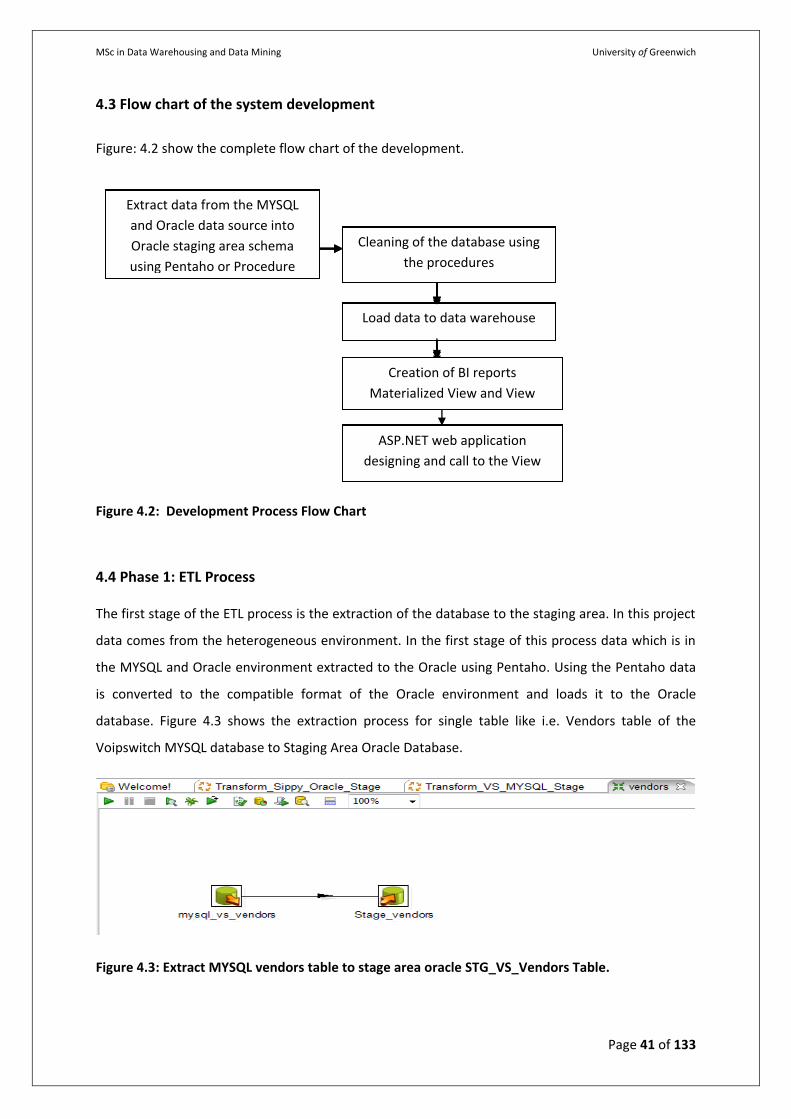
MSc in Data Warehousing and Data Mining University of Greenwich
Page 41 of 133
4.3 Flow chart of the system development
Figure: 4.2 show the complete flow chart of the development.
Figure 4.2: Development Process Flow Chart
4.4 Phase 1: ETL Process
The first stage of the ETL process is the extraction of the database to the staging area. In this project
data comes from the heterogeneous environment. In the first stage of this process data which is in
the MYSQL and Oracle environment extracted to the Oracle using Pentaho. Using the Pentaho data
is converted to the compatible format of the Oracle environment and loads it to the Oracle
database. Figure 4.3 shows the extraction process for single table like i.e. Vendors table of the
Voipswitch MYSQL database to Staging Area Oracle Database.
Figure 4.3: Extract MYSQL vendors table to stage area oracle STG_VS_Vendors Table.
Creation of BI reports procedures
Cleaning of the database using
the procedures
Cleaning of the database using
the procedures
Load data to data warehouse
Cleaning of the database using
the procedures
Both database integration in Sql
server using the procedures
Cleaning of the database using
the procedures
Extract data from the access
into MS SQLSever Cleaning of the database using
the procedures
Windows form designing and call
procedures to forms
Creation of BI reports procedures
Load data to data warehouse
ASP.NET web application
designing and call to the View
Creation of BI reports
Materialized View and View
Load data to data warehouse
Cleaning of the database using
the procedures
Extract data from the MYSQL
and Oracle data source into
Oracle staging area schema
using Pentaho or Procedure
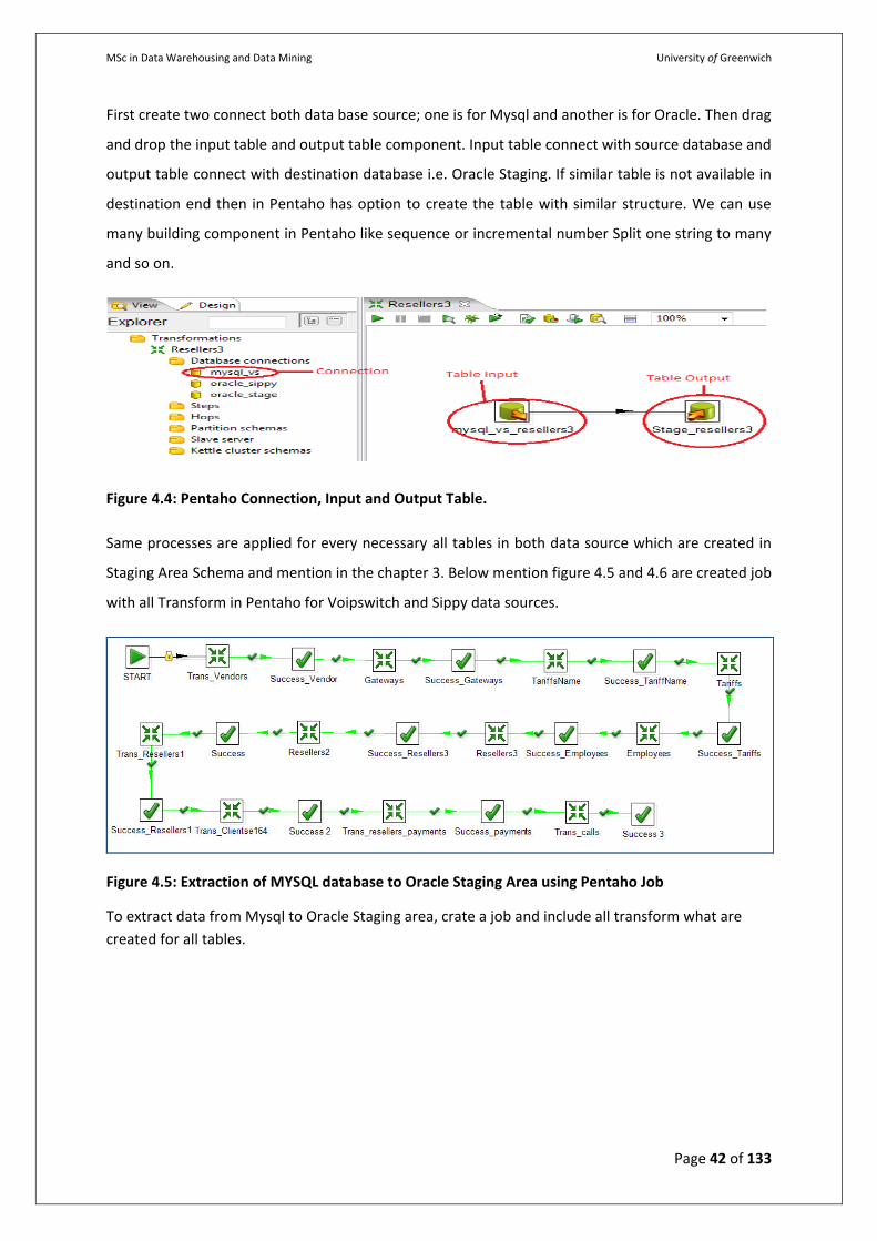
MSc in Data Warehousing and Data Mining University of Greenwich
Page 42 of 133
First create two connect both data base source; one is for Mysql and another is for Oracle. Then drag
and drop the input table and output table component. Input table connect with source database and
output table connect with destination database i.e. Oracle Staging. If similar table is not available in
destination end then in Pentaho has option to create the table with similar structure. We can use
many building component in Pentaho like sequence or incremental number Split one string to many
and so on.
Figure 4.4: Pentaho Connection, Input and Output Table.
Same processes are applied for every necessary all tables in both data source which are created in
Staging Area Schema and mention in the chapter 3. Below mention figure 4.5 and 4.6 are created job
with all Transform in Pentaho for Voipswitch and Sippy data sources.
Figure 4.5: Extraction of MYSQL database to Oracle Staging Area using Pentaho Job
To extract data from Mysql to Oracle Staging area, crate a job and include all transform what are
created for all tables.
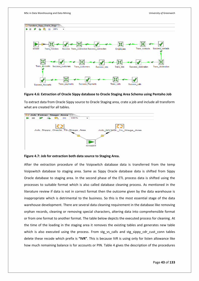
MSc in Data Warehousing and Data Mining University of Greenwich
Page 43 of 133
Figure 4.6: Extraction of Oracle Sippy database to Oracle Staging Area Schema using Pentaho Job
To extract data from Oracle Sippy source to Oracle Staging area, crate a job and include all transform
what are created for all tables.
Figure 4.7: Job for extraction both data source to Staging Area.
After the extraction procedure of the Voipswitch database data is transferred from the temp
Voipswitch database to staging area. Same as Sippy Oracle database data is shifted from Sippy
Oracle database to staging area. In the second phase of the ETL process data is shifted using the
processes to suitable format which is also called database cleaning process. As mentioned in the
literature review if data is not in correct format then the outcome given by the data warehouse is
inappropriate which is detrimental to the business. So this is the most essential stage of the data
warehouse development. There are several data cleaning requirement in the database like removing
orphan records, cleaning or removing special characters, altering data into comprehensible format
or from one format to another format. The table below depicts the executed process for cleaning. At
the time of the loading in the staging area it removes the existing tables and generates new table
which is also executed using the process. From stg_vs_calls and stg_sippy_cdr_cust_conn tables
delete these recode which prefix is “IVR”. This is because IVR is using only for listen allowance like
how much remaining balance is for accounts or PIN. Table 4 gives the description of the procedures
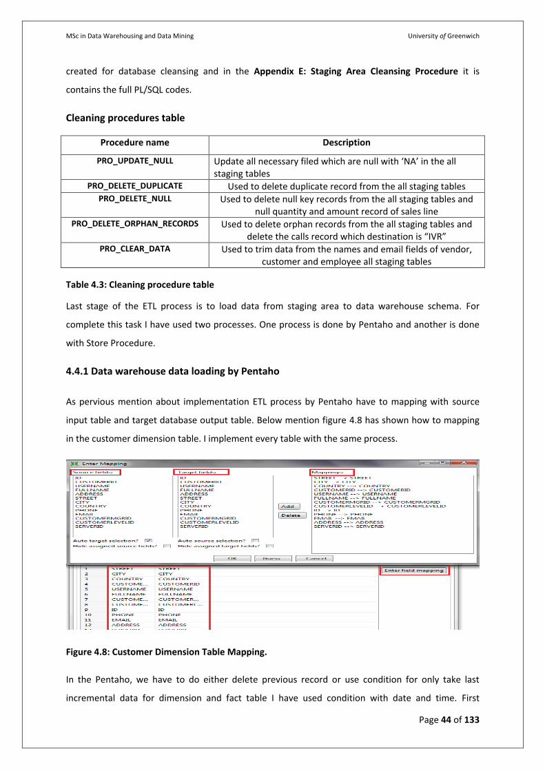
MSc in Data Warehousing and Data Mining University of Greenwich
Page 44 of 133
created for database cleansing and in the Appendix E: Staging Area Cleansing Procedure it is
contains the full PL/SQL codes.
Cleaning procedures table
Procedure name Description
PRO_UPDATE_NULL Update all necessary filed which are null with ‘NA’ in the all staging tables
PRO_DELETE_DUPLICATE Used to delete duplicate record from the all staging tables PRO_DELETE_NULL Used to delete null key records from the all staging tables and
null quantity and amount record of sales line PRO_DELETE_ORPHAN_RECORDS Used to delete orphan records from the all staging tables and
delete the calls record which destination is “IVR” PRO_CLEAR_DATA Used to trim data from the names and email fields of vendor,
customer and employee all staging tables
Table 4.3: Cleaning procedure table
Last stage of the ETL process is to load data from staging area to data warehouse schema. For
complete this task I have used two processes. One process is done by Pentaho and another is done
with Store Procedure.
4.4.1 Data warehouse data loading by Pentaho
As pervious mention about implementation ETL process by Pentaho have to mapping with source
input table and target database output table. Below mention figure 4.8 has shown how to mapping
in the customer dimension table. I implement every table with the same process.
Figure 4.8: Customer Dimension Table Mapping.
In the Pentaho, we have to do either delete previous record or use condition for only take last
incremental data for dimension and fact table I have used condition with date and time. First
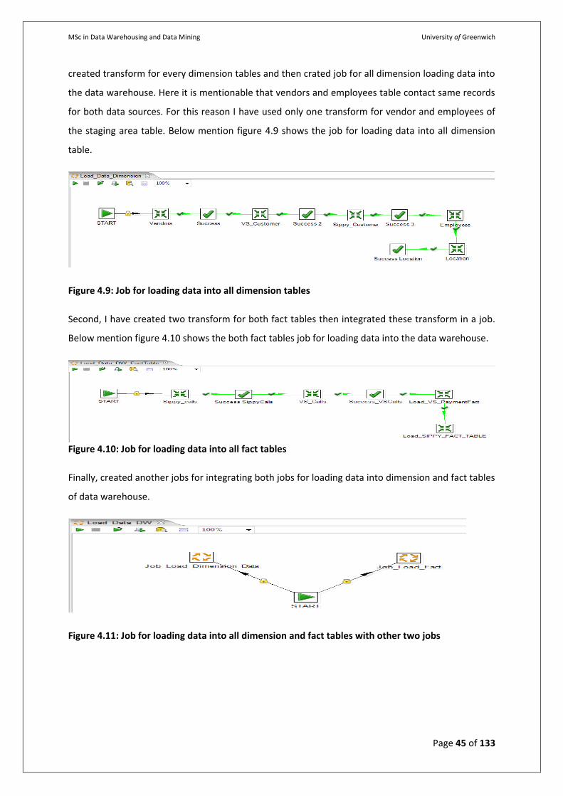
MSc in Data Warehousing and Data Mining University of Greenwich
Page 45 of 133
created transform for every dimension tables and then crated job for all dimension loading data into
the data warehouse. Here it is mentionable that vendors and employees table contact same records
for both data sources. For this reason I have used only one transform for vendor and employees of
the staging area table. Below mention figure 4.9 shows the job for loading data into all dimension
table.
Figure 4.9: Job for loading data into all dimension tables
Second, I have created two transform for both fact tables then integrated these transform in a job.
Below mention figure 4.10 shows the both fact tables job for loading data into the data warehouse.
Figure 4.10: Job for loading data into all fact tables
Finally, created another jobs for integrating both jobs for loading data into dimension and fact tables
of data warehouse.
Figure 4.11: Job for loading data into all dimension and fact tables with other two jobs
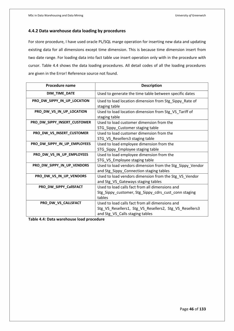
MSc in Data Warehousing and Data Mining University of Greenwich
Page 46 of 133
4.4.2 Data warehouse data loading by procedures
For store procedure, I have used oracle PL/SQL marge operation for inserting new data and updating
existing data for all dimensions except time dimension. This is because time dimension insert from
two date range. For loading data into fact table use insert operation only with in the procedure with
cursor. Table 4.4 shows the data loading procedures. All detail codes of all the loading procedures
are given in the Error! Reference source not found.
Procedure name Description
DIM_TIME_DATE Used to generate the time table between specific dates
PRO_DW_SIPPY_IN_UP_LOCATION Used to load location dimension from Stg_Sippy_Rate of staging table
PRO_DW_VS_IN_UP_LOCATION Used to load location dimension from Stg_VS_Tariff of staging table
PRO_DW_SIPPY_INSERT_CUSTOMER Used to load customer dimension from the STG_Sippy_Customer staging table
PRO_DW_VS_INSERT_CUSTOMER Used to load customer dimension from the STG_VS_Resellers3 staging table
PRO_DW_SIPPY_IN_UP_EMPLOYEES Used to load employee dimension from the STG_Sippy_Employee staging table
PRO_DW_VS_IN_UP_EMPLOYEES Used to load employee dimension from the STG_VS_Employee staging table
PRO_DW_SIPPY_IN_UP_VENDORS Used to load vendors dimension from the Stg_Sippy_Vendor and Stg_Sippy_Connection staging tables
PRO_DW_VS_IN_UP_VENDORS Used to load vendors dimension from the Stg_VS_Vendor and Stg_VS_Gateways staging tables
PRO_DW_SIPPY_CallSFACT Used to load calls fact from all dimensions and Stg_Sippy_customer, Stg_Sippy_cdrs_cust_conn staging tables
PRO_DW_VS_CALLSFACT Used to load calls fact from all dimensions and Stg_VS_Resellers1, Stg_VS_Resellers2, Stg_VS_Resellers3 and Stg_VS_Calls staging tables
Table 4.4: Data warehouse load procedure
MSc in Data Warehousing and Data Mining University of Greenwich
Page 47 of 133
Chapter 5
Implement Data Visualisation for BI
5.1 Overview
“Development stage emphases on how data are to be organized, how functions and techniques are
to be applied in the software architecture” (PRESSMAN, Roger S, 2004). This chapter demonstrates
the information about the implementation of the system which comprises the technology used for
application and the finalized reports discussion. In the start of this chapter it gives the explanation of
the tools used for Silverlight ASP.NET web Application. In the last it describes the finalized report
which is produced in the ASP.NET web Application using the Silverlight Tool Kit and ODP.
5.2.1 ASP.NET Application 2010 (C#)
ASP.NET Web based application are the name given by the Microsoft and it is the graphical API
delivered with .Net framework with Silverlight Tool Kit. Developer can enhance and remove controls
to manipulate data with the drag and drop or by doing some variations in the code. With practice of
the drag and drop functionalities and the easy to use graphical interface developer can make the
solution in a faster and easier way. In these project web pages are used to develop the user interface
to get the output of the reports. (MICROSOFT)
5.2.2. Entity Framework
When one have a view at the size of code that the average application developer must write to
address the impedance mismatch across different data representations it is clear that there is a
chance for upgrading. Without a doubt, there are many scenarios where the right framework can
allow an application developer to focus on the requirements of the application as opposed to the
complexities of connecting contrasting data representations.
A key objective of the forthcoming version of ADO.NET is to increase the level of abstraction for data
programming, thus serving to reduce the impedance mismatch between data models and between
languages that application developers would otherwise have to deal with. Two innovations that
make this step promising are Language-Integrated Query and the ADO.NET Entity Framework. The
Entity Framework exists as a new part of the ADO.NET family of technologies. (MICROSOFT)
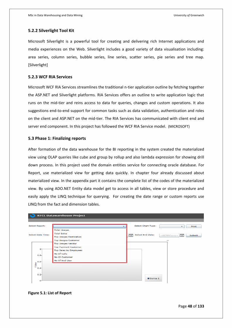
MSc in Data Warehousing and Data Mining University of Greenwich
Page 48 of 133
5.2.2 Silverlight Tool Kit
Microsoft Silverlight is a powerful tool for creating and delivering rich Internet applications and
media experiences on the Web. Silverlight includes a good variety of data visualisation including:
area series, column series, bubble series, line series, scatter series, pie series and tree map.
[Silverlight]
5.2.3 WCF RIA Services
Microsoft WCF RIA Services streamlines the traditional n-tier application outline by fetching together
the ASP.NET and Silverlight platforms. RIA Services offers an outline to write application logic that
runs on the mid-tier and reins access to data for queries, changes and custom operations. It also
suggestions end-to-end support for common tasks such as data validation, authentication and roles
on the client and ASP.NET on the mid-tier. The RIA Services has communicated with client end and
server end component. In this project has followed the WCF RIA Service model. (MICROSOFT)
5.3 Phase 1: Finalizing reports
After formation of the data warehouse for the BI reporting in the system created the materialized
view using OLAP queries like cube and group by rollup and also lambda expression for showing drill
down process. In this project used the domain entities service for connecting oracle database. For
Report, use materialized view for getting data quickly. In chapter four already discussed about
materialized view. In the appendix part it contains the complete list of the codes of the materialized
view. By using ADO.NET Entity data model get to access in all tables, view or store procedure and
easily apply the LINQ technique for querying. For creating the date range or custom reports use
LINQ from the fact and dimension tables.
Figure 5.1: List of Report
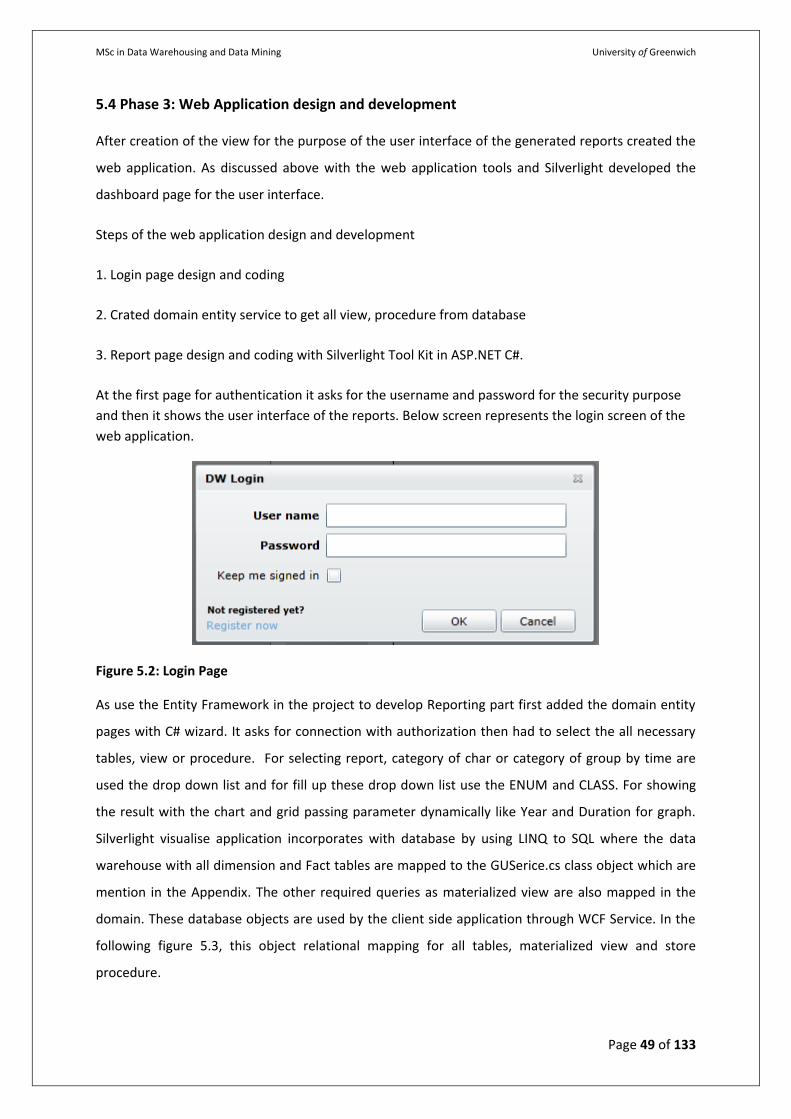
MSc in Data Warehousing and Data Mining University of Greenwich
Page 49 of 133
5.4 Phase 3: Web Application design and development
After creation of the view for the purpose of the user interface of the generated reports created the
web application. As discussed above with the web application tools and Silverlight developed the
dashboard page for the user interface.
Steps of the web application design and development
1. Login page design and coding
2. Crated domain entity service to get all view, procedure from database
3. Report page design and coding with Silverlight Tool Kit in ASP.NET C#.
At the first page for authentication it asks for the username and password for the security purpose
and then it shows the user interface of the reports. Below screen represents the login screen of the
web application.
Figure 5.2: Login Page
As use the Entity Framework in the project to develop Reporting part first added the domain entity
pages with C# wizard. It asks for connection with authorization then had to select the all necessary
tables, view or procedure. For selecting report, category of char or category of group by time are
used the drop down list and for fill up these drop down list use the ENUM and CLASS. For showing
the result with the chart and grid passing parameter dynamically like Year and Duration for graph.
Silverlight visualise application incorporates with database by using LINQ to SQL where the data
warehouse with all dimension and Fact tables are mapped to the GUSerice.cs class object which are
mention in the Appendix. The other required queries as materialized view are also mapped in the
domain. These database objects are used by the client side application through WCF Service. In the
following figure 5.3, this object relational mapping for all tables, materialized view and store
procedure.
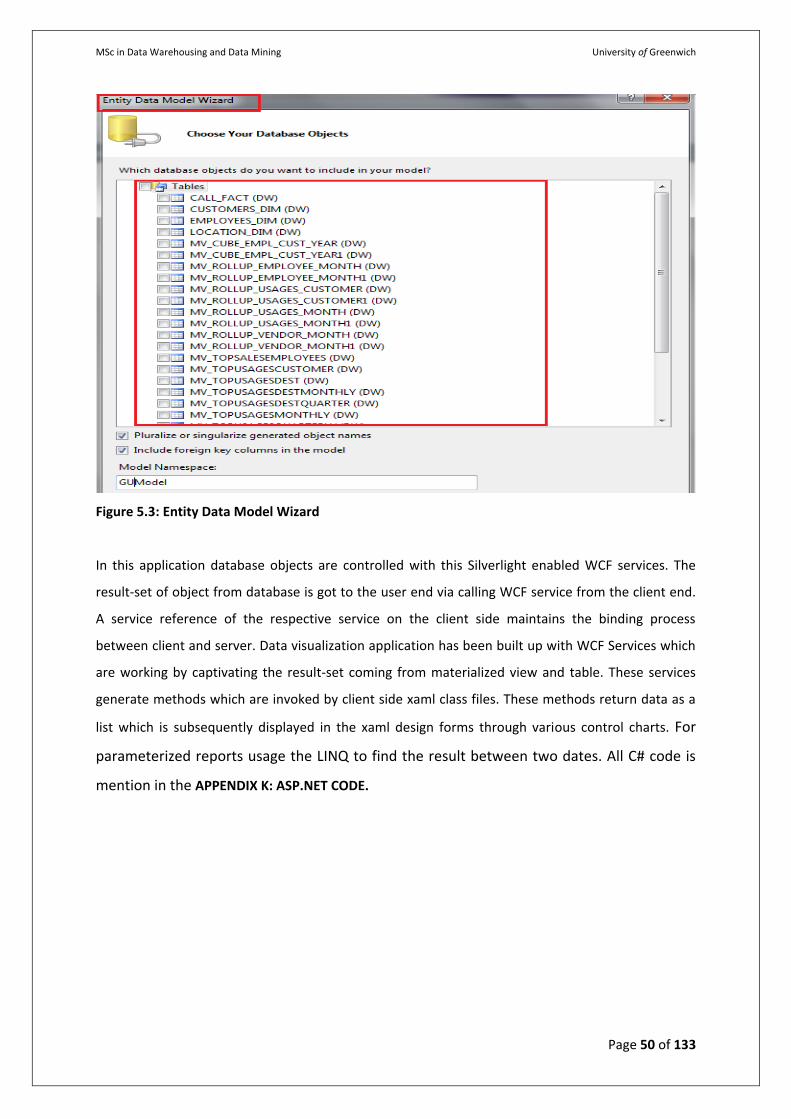
MSc in Data Warehousing and Data Mining University of Greenwich
Page 50 of 133
Figure 5.3: Entity Data Model Wizard
In this application database objects are controlled with this Silverlight enabled WCF services. The
result-set of object from database is got to the user end via calling WCF service from the client end.
A service reference of the respective service on the client side maintains the binding process
between client and server. Data visualization application has been built up with WCF Services which
are working by captivating the result-set coming from materialized view and table. These services
generate methods which are invoked by client side xaml class files. These methods return data as a
list which is subsequently displayed in the xaml design forms through various control charts. For
parameterized reports usage the LINQ to find the result between two dates. All C# code is
mention in the APPENDIX K: ASP.NET CODE.
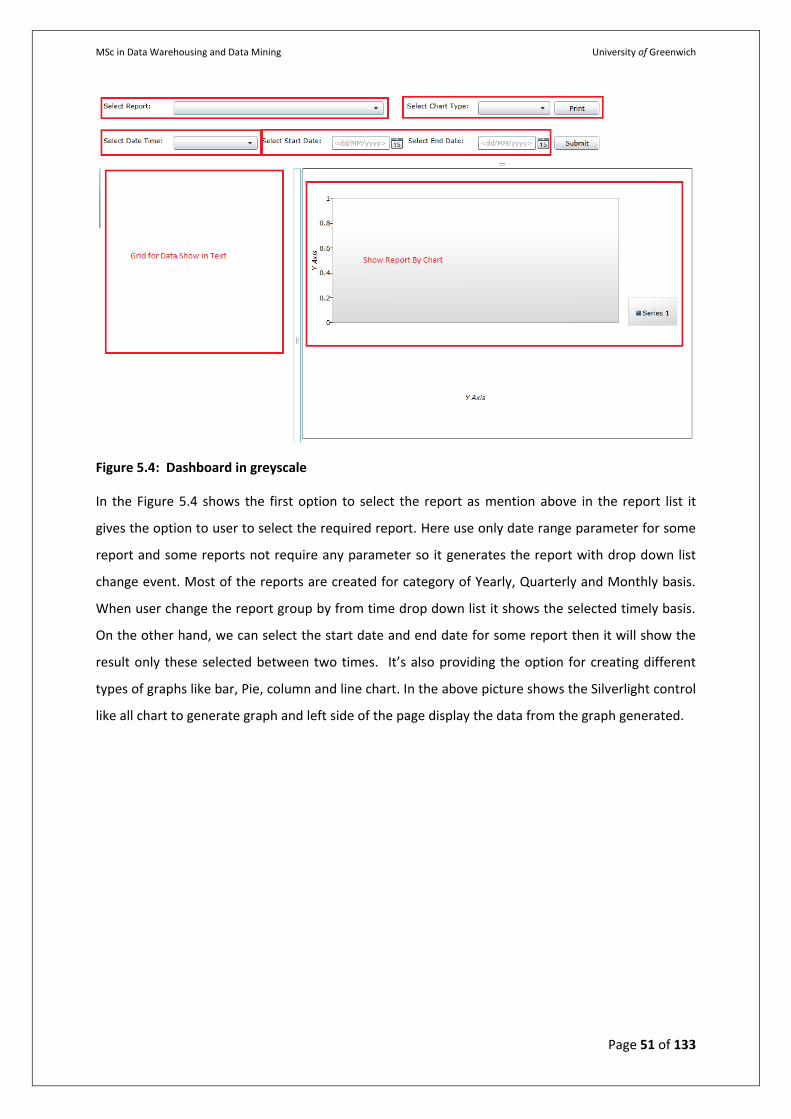
MSc in Data Warehousing and Data Mining University of Greenwich
Page 51 of 133
Figure 5.4: Dashboard in greyscale
In the Figure 5.4 shows the first option to select the report as mention above in the report list it
gives the option to user to select the required report. Here use only date range parameter for some
report and some reports not require any parameter so it generates the report with drop down list
change event. Most of the reports are created for category of Yearly, Quarterly and Monthly basis.
When user change the report group by from time drop down list it shows the selected timely basis.
On the other hand, we can select the start date and end date for some report then it will show the
result only these selected between two times. It’s also providing the option for creating different
types of graphs like bar, Pie, column and line chart. In the above picture shows the Silverlight control
like all chart to generate graph and left side of the page display the data from the graph generated.
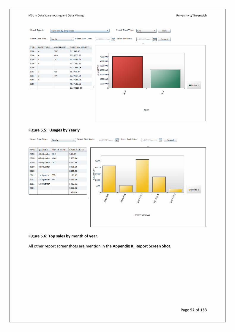
MSc in Data Warehousing and Data Mining University of Greenwich
Page 52 of 133
Figure 5.5: Usages by Yearly
Figure 5.6: Top sales by month of year.
All other report screenshots are mention in the Appendix K: Report Screen Shot.
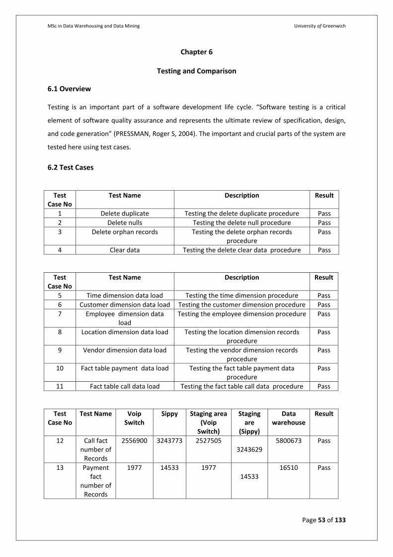
MSc in Data Warehousing and Data Mining University of Greenwich
Page 53 of 133
Chapter 6
Testing and Comparison
6.1 Overview
Testing is an important part of a software development life cycle. “Software testing is a critical
element of software quality assurance and represents the ultimate review of specification, design,
and code generation” (PRESSMAN, Roger S, 2004). The important and crucial parts of the system are
tested here using test cases.
6.2 Test Cases
Test Case No
Test Name Description Result
1 Delete duplicate Testing the delete duplicate procedure Pass
2 Delete nulls Testing the delete null procedure Pass
3 Delete orphan records Testing the delete orphan records procedure
Pass
4 Clear data Testing the delete clear data procedure Pass
Test Case No
Test Name Description Result
5 Time dimension data load Testing the time dimension procedure Pass
6 Customer dimension data load Testing the customer dimension procedure Pass
7 Employee dimension data load
Testing the employee dimension procedure Pass
8 Location dimension data load Testing the location dimension records procedure
Pass
9 Vendor dimension data load Testing the vendor dimension records procedure
Pass
10 Fact table payment data load Testing the fact table payment data procedure
Pass
11 Fact table call data load Testing the fact table call data procedure Pass
Test Case No
Test Name Voip Switch
Sippy Staging area (Voip
Switch)
Staging are
(Sippy)
Data warehouse
Result
12 Call fact number of
Records
2556900 3243773 2527505 3243629
5800673 Pass
13 Payment fact
number of Records
1977 14533 1977 14533
16510 Pass
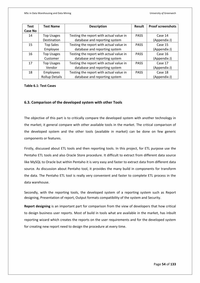
MSc in Data Warehousing and Data Mining University of Greenwich
Page 54 of 133
Test Case No
Test Name Description Result Proof screenshots
14 Top Usages Destination
Testing the report with actual value in database and reporting system
PASS Case 14 (Appendix J)
15 Top Sales Employee
Testing the report with actual value in database and reporting system
PASS Case 15 (Appendix J)
16 Top Usages Customer
Testing the report with actual value in database and reporting system
PASS Case 16 (Appendix J)
17 Top Usages Vendor
Testing the report with actual value in database and reporting system
PASS Case 17 (Appendix J)
18 Employees Rollup Details
Testing the report with actual value in database and reporting system
PASS Case 18 (Appendix J)
Table 6.1: Test Cases
6.3. Comparison of the developed system with other Tools
The objective of this part is to critically compare the developed system with another technology in
the market; it general compare with other available tools in the market. The critical comparison of
the developed system and the other tools (available in market) can be done on few generic
components or features.
Firstly, discussed about ETL tools and then reporting tools. In this project, for ETL purpose use the
Pentaho ETL tools and also Oracle Store procedure. It difficult to extract from different data source
like MySQL to Oracle but within Pentaho it is very easy and faster to extract data from different data
source. As discussion about Pentaho tool, it provides the many build in components for transform
the data. The Pentaho ETL tool is really very convenient and faster to complete ETL process in the
data warehouse.
Secondly, with the reporting tools, the developed system of a reporting system such as Report
designing, Presentation of report, Output formats compatibility of the system and Security.
Report designing is an important part for comparison from the view of developers that how critical
to design business user reports. Most of build in tools what are available in the market, has inbuilt
reporting wizard which creates the reports on the user requirements and for the developed system
for creating new report need to design the procedure at every time.
MSc in Data Warehousing and Data Mining University of Greenwich
Page 55 of 133
Presentation of report with the built in software once the report design is done the user cannot
change the graphical representation of the report but for the developed system it provides the
option to change the graphical view. Most of build-in software is support 3 dimensional view of the
report but in the developed system the presentation is limited to two dimensional views. But with
the Silverlight it is possible to do report with 3 dimensional views. In this project used the Silverlight
4 tool kit. For 3 dimension view everything has to do manually via XAML code. As future work,
mentioned for implementing about the 3 dimension view report.
Output formats is a sensitive part in any business user report as the user need to understand the
report format, for build in toots is provide facility to export generated report in Microsoft office or
PDF format, for the developed system its provide to print or save generated graph in the PDF format.
Security for the security purposes the developed system provides the login, the other tools we can
also create or using the login feature.
MSc in Data Warehousing and Data Mining University of Greenwich
Page 56 of 133
Chapter 7
Evaluation and Future work
7.1 Overview
In the development parts of this project attempts to attain the best part of the solution and try to
practise the best technology as many as possible. This chapter narrates the technological and
application assessment and what future modifications can be possible for the each stage of the
development course.
7.2 Phase 1
In the phase 1 of development process the Implementation of Data Warehouse is completed. Now
RTCL’s is introducing to run all department with computerized like HR, customer complain
management and accounts. In future, all other department could be integrated as data mart in data
warehouse.
7.3 Phase 2
In the phase 2 of the development process the ETL process is completed provided that database
using the PL/SQL processes and the Pentaho ETL tool. As we know that technology has become more
and more advanced and in the market there are additional number of tools existing for ETL process
which can do it quickly and easily. In the present procedure the ETL part of the development by
Pentaho ETL Tool and Store Procedure. Data cleansing procedure and data loading in data
warehouse is also developed by PL/SQL store procedure which is entirely manual procedure and
developer needs to do all the process manually, such as, developer needs to go to each procedure
and run it manually. In the future, we can do the batch processing of the all necessary procedure and
Pentaho Tool can set up the time to run automatically so whenever the new data will be available
then it can get it to the data warehouse.
7.4 Phase 3
In the phase 3 of the development process the reports materialized view is finalized with OLAO
query like CUBE AND ROLLUP option which finds out the report’s data from the database and refers
it to the front end environment for user view. Since, in the existing development for each table there
is a separate materialized view to find out the report data. In this part as future development can
MSc in Data Warehousing and Data Mining University of Greenwich
Page 57 of 133
make process which can take the date range from the user. The current developed system show the
report with 2 dimension view. In future development can possible to do with 3 dimension view.
7.5 Phase 4
In the phase 4 of the development process the web application is created for the user interface
which lets the user to login in the reporting system and select the report which offers the
information about the sales and provide the user in the form of graphs and the text format. In this
phase can do the more improvements like providing the user to decide on the attribute of every
dimension and generate the selection of report by sales or usages? So with the use of this reporting
can be more dynamic.
MSc in Data Warehousing and Data Mining University of Greenwich
Page 58 of 133
Chapter 8
Conclusion
8.1 General conclusion
The developed Data Warehouse and Data Visualisation for BI solution offers the basic simple
application necessity but there would be still lot more improvements in the developed solution
necessary as compared to the existing BI solution in the market. The main objective of the project is
to implement data warehouse and provide the primary data visualisation for BI reporting system
which is attained at the end of the project.
Challenges are confronted during the design part of the design and development segment of the
project. In the design section of the project it is truly hard to finalize the data warehouse design as
the data comes from the two different sources and the database provided is not in appropriate
format. But with the help of the notes of the past studied section in my post-graduation and with
the help of my supervisor it was possible to finalize the good design of the data warehouse. In the
development section as in the project used the processes to develop the reports and also for the
cleaning of database. During the development of the procedure and the user interface tackled many
types casting and format mismatching problems. With the use of the web materials it was possible
find out the solution and sometime it needed to change in the design of the database view. In the
last part of the development design the user interface using the web application which is totally
database dependant so some difficulties met during the design of it to call the procedure and to pass
the parameter to procedure. Depending on the requirement, the forms changed the design of the
procedures.
8.2 Personal Experience
It is a great opportunity for me that I have got a chance to design and develop a project of this scale.
During the development of the project I got extraordinary support from my supervisor and tutors of
the university. At the beginning of this project I had little experience about data warehouse, ETL and
BI Reporting, Silverlight and Pentaho which are used for the development of the project though I had
experience in ASP.NET and Database Management and programming with PL/SQL. It was really a
superb learning experience for me leading to get the knowledge about the implementation of data
warehouse and data visualisation for BI. It was really a challenging and enjoying project because for
this project I had to learn in depth about to development of Data Warehouse, ETL and BI Reporting.
MSc in Data Warehousing and Data Mining University of Greenwich
Page 59 of 133
References Anahory, S and Murray, D., (1997). Data Warehousing in the Real World. New York: Addison Wesley. Ballard, C; Herreman, D; Schau, D; Bell, R; Kim, E and Valencic, A., (1998). Data Modelling techniques for data warehousing. IBM Redbooks. Available from: http://www.redbooks.ibm.com/redbooks/pdfs/sg242238.pdf [Accessed 30th July 2011]. Bonifati, A; Cattaneo, F; Ceri, S; Fuggetta, A and Paraboschi, S., (2001). Designing data marts for data warehouses. ACM Transactions on Software Engineering and Methodology, 10 (4), 452-483. Chaudhuri, S and Dayal, U., (1997). An overview of data warehousing and OLAP technology. ACM SIGMOD Record, 26 (1), 65-74. Chenoweth, T ; Schuff, D and St.Louis, R., (2003). A method for developing dimensional data marts. Communications of the ACM, 46(12), 93-98. Colliat, G., (1996). OLAP, relational and multidimensional database systems. ACM SIGMOD, 25(3), 64-69. Connolly, T and Begg, C., (2002). Database systems. A practical approach to design, implementation, and management. 3rd ed. New York: Addison Wesley. Dash, A and Agarwal, R., (2001). Dimensional modelling for a data warehouse. ACM SIGSOFT Software Engineering Notes, 26(6), 83 -84. Datta, A and Thomas, H., (1999). The cube data model: a conceptual model and algebra for on-line analytical processing in data warehouses. Decision Support Systems, 27(3), 289-301. David Adams,Accenture. (n.d.). data visualization. Retrieved August 25, 2011, from
www.cfoporject.com.
Devlin, B and Murphy, P., (1988). Architecture for a business and information system, IBM Systems Journal, 27 (1), 60-80. Drewek, K., (2005). Data Warehouse Architecture: The Great Debate. Available from: http://www.b-eye-network.com/view/693 [Accessed 12th July 2011]. Eckerson, W., (2007). Four Ways to Build a Data Warehouse. Available from: http://www.tdan.com/view-articles/4770 [Accessed 30th October 2011].
ETL_Comparison. (n.d.). Retrieved august 12, 2011, from www.lookouster.org:
http://lookouster.org/blog/files/etl_cmp.pdf
Etl_tool_comparison. (n.d.). Retrieved august 27, 2011, from www.pentaho.com:
http://www.pentaho.com/docs/informatica_pentaho_etl_tools_comparison.pdf
Giorgini, P; Rizzi, S and Garzetti, M., (2005). Goal-oriented requirement analysis for data
MSc in Data Warehousing and Data Mining University of Greenwich
Page 60 of 133
warehouse design. Proceedings of the 8th ACM international workshop on Data warehousing and OLAP. New York, ACM Press, 47-56. Golfarelli, M; Lechtenbörger, J; Rizzi, S and Vossen, G., (2006). Schema versioning in data warehouses: Enabling cross-version querying via schema augmentation. Data & Knowledge Engineering, In Press. Golfarelli, M and Rizzi, S., (1998). A methodological framework for data warehouse design. Proceedings of the 1st ACM international workshop on Data warehousing and OLAP. New York, ACM press, 3-9. Huang,C ; Tseng, T ; Li, M and Gung,R., (2005). Models of multi-dimensional analysis for qualitative data and its application. European Journal of Operational Research. In Press. Hurtado, C and Mendelzon, A., (2002). OLAP dimension constraints. Proceedings of the 21st ACM SIGMOD-SIGACT-SIGART symposium on Principles of database systems. New York, ACM press, 169-179. IBM (n,d), Starflake Schema Available from: http://publib.boulder.ibm.com/infocenter/rdahelp/v7r5/index.jsp?topic=%2Fcom.ibm.datatools.dimensional.ui.doc%2Ftopics%2Fc_dm_snowflake_schemas.html [Accessed 30th October 2011]. Inmon, W; Imhoff, C and Sousa, R., (2000). Corporate Information Factory. 2nd ed. New York: Wiley. Inmon, W., (1996). The data warehouse and data mining. Communications of the ACM, 39(11),49-50. Jones, M and Song, I., (2005). Dimensional modelling: identifying, classifying & applying patterns. Proceedings of the 8th ACM international workshop on Data warehousing and OLAP. New York, ACM Press, 29-38. Kaser, O and Lemire, D., (2005). Attribute value reordering for efficient hybrid OLAP. Available from: http://www.daniel-lemire.com/fr/documents/publications/is2004_web.pdf [Accessed 12 October 2011]. Kimball, R., (2001). Kimball Design Tip #2: Variable Depth Customer Dimensions. Available from: http://www.kimballgroup.com/html/designtipsPDF/DesignTips2001/KimballDT22VariableDepth.pdf [Accessed on: 2nd December 2011]. Kimball, R; Reeves, L; Ross, M and Thornthwaite, W., (1998). The Data Warehouse Lifecycle Toolkit. New York: Wiley. Kimball, R., (1996). The data warehouse toolkit: practical techniques for building dimensional data warehouses. New York: Wiley. Krippendorf, M and Song, I., (1997). The Translation of Star Schema into Entity-Relationship Diagrams. DEXA workshop. Available from: http://www.olap.it/Articoli/StarSchemato3NFtranslation.pdf [Accessed on: 20 November 2011].
MSc in Data Warehousing and Data Mining University of Greenwich
Page 61 of 133
Lu, X and Lowenthal, F., (2004). Arranging fact table records in a data warehouse to improve query performance. Computers & Operations Research, 31(13), 2165-2182. Mailvaganam, H., (2004). Data Warehouse Design: Design Methodologies of Kimball and Inmon...Plus a Third Way. Available from: http://www.dwreview.com/Articles/KimballInmon.html [Accessed 30th October 2011]. Malinowski, E and Zimányi, E., (2005). Hierarchies in a multidimensional model: From conceptual modeling to logical representation. Data & Knowledge Engineering. In Press. Geographic information systems. New York, ACM Press, 12-22. Martyn, T., (2004). Reconsidering Multi-Dimensional schemas. ACM SIGMOD Record, 33(1), 83-88.
Michael Friendly (2008). “Milestones in the history of thematic cartography, statistical graphics, and
data visualization”.
Microsoft (n.d.). Retrieved Jan 22, 2012, from www.microsoft.com:
http://www.microsoft.com/download/en/details.aspx?id=14880
Pentaho Data Integration (n.d.). Retrieved December 27, 2011, from www.pentaho.com:
http://www.pentaho.com/docs/pentaho_data_integration.pdf
Pentaho Architecture (n.d.). Retrieved December 27, 2011, from www.pentaho.com: http://wiki.pentaho.com/display/COM/Architecture Pressman, R. S. (2004). Software engineering : a practitioner's approach. Boston, [Mass.] ; London :
McGraw-Hill Higher Education.
Pokorny, J., (2001). Modelling stars using XML. Proceedings of the 4th ACM international workshop on Data warehousing and OLAP. New York, ACM Press, 24-31. Ponniah, P., (2001). Data warehousing Fundamentals: A comprehensive Guide for IT Professionals. New York: Wiley. Priebe, T and Pernul, G., (2000). Towards OLAP security design — survey and research issues. Proceedings of the 3rd ACM international workshop on Data warehousing and OLAP. New York, ACM Press, 33-40. Saharia, A and Babad, Y., (2000). Enhancing Data Warehouse performance through query caching. ACM SIGMIS Database, 31(3), 43-63. Silverlight (n.d.) www.silverlight.net. [online]. [Accessed 20 Jan 2012]. Available from World Wide Web: < http://www.silverlight.net> Singhal, A., (2004). Design of a data warehouse system for network/web services. Proceedings of the thirteenth ACM conference on information and knowledge management.
MSc in Data Warehousing and Data Mining University of Greenwich
Page 62 of 133
New York, ACM Press, 473-476. Sprial Lifecycle Model (n.d.). Retrieved December 30, 2011, from http://www.softdevteam.com/Spiral-lifecycle.asp Summer, E and Ali, D., (1996). A practical guide for implementing data warehousing. Computers & Industrial Engineering, 31(1-2), 307-310. Theodoratos, D; Ligoudistianos, S and Sellis, T., (2001). View selection for designing the global data warehouse. Data & Knowledge Engineering, 39(3), 219-240. Tryfona, N; Busborg, F and Christiansen, J., (1999). StarER: a conceptual model for data warehouse design. Proceedings of the 2nd ACM international workshop on Data warehousing and OLAP. New York, ACM Press, 3-8. Vassiliadis, P and Sellis, T., (1999). A survey of logical models for OLAP databases. ACM SIGMOD Record, 28(4), 64-69. Watson, H; Goodhue, H and Wixom, B., (2002). The benefits of data warehousing: why some organizations realize exceptional payoffs. Information & Management, 39 (6), 491-502. Weininger, A., (2002). Efficient execution of joins in a star schema. Proceedings of the 2002 ACM SIGMOD international conference on Management of data. New York, ACM Press, 542-545.
Vitaly Friedman (2008) Data Visualization and Infographics in: Graphics, Monday Inspiration, January
14th, 2008.
MSc in Data Warehousing and Data Mining University of Greenwich
Page 63 of 133
Appendix A:
Confidential Disclosure Agreement
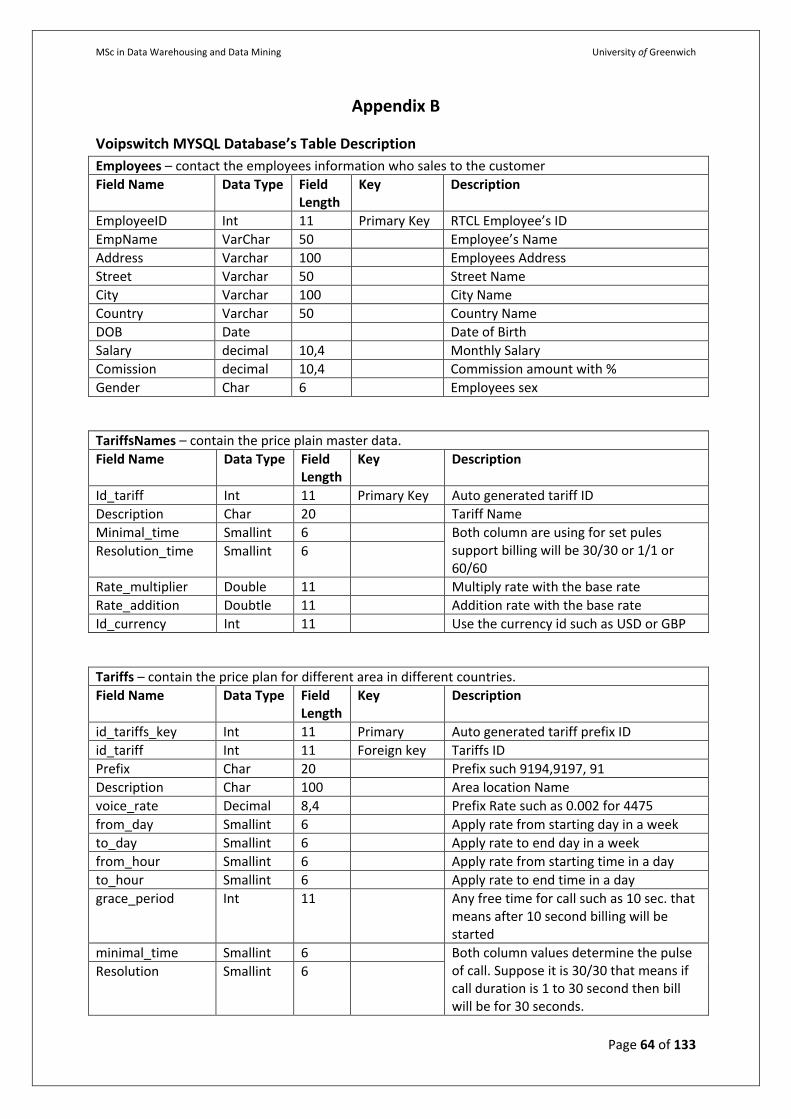
MSc in Data Warehousing and Data Mining University of Greenwich
Page 64 of 133
Appendix B
Voipswitch MYSQL Database’s Table Description
Employees – contact the employees information who sales to the customer
Field Name Data Type Field Length
Key Description
EmployeeID Int 11 Primary Key RTCL Employee’s ID
EmpName VarChar 50 Employee’s Name
Address Varchar 100 Employees Address
Street Varchar 50 Street Name
City Varchar 100 City Name
Country Varchar 50 Country Name
DOB Date Date of Birth
Salary decimal 10,4 Monthly Salary
Comission decimal 10,4 Commission amount with %
Gender Char 6 Employees sex
TariffsNames – contain the price plain master data.
Field Name Data Type Field Length
Key Description
Id_tariff Int 11 Primary Key Auto generated tariff ID
Description Char 20 Tariff Name
Minimal_time Smallint 6 Both column are using for set pules support billing will be 30/30 or 1/1 or 60/60
Resolution_time Smallint 6
Rate_multiplier Double 11 Multiply rate with the base rate
Rate_addition Doubtle 11 Addition rate with the base rate
Id_currency Int 11 Use the currency id such as USD or GBP
Tariffs – contain the price plan for different area in different countries.
Field Name Data Type Field Length
Key Description
id_tariffs_key Int 11 Primary Auto generated tariff prefix ID
id_tariff Int 11 Foreign key Tariffs ID
Prefix Char 20 Prefix such 9194,9197, 91
Description Char 100 Area location Name
voice_rate Decimal 8,4 Prefix Rate such as 0.002 for 4475
from_day Smallint 6 Apply rate from starting day in a week
to_day Smallint 6 Apply rate to end day in a week
from_hour Smallint 6 Apply rate from starting time in a day
to_hour Smallint 6 Apply rate to end time in a day
grace_period Int 11 Any free time for call such as 10 sec. that means after 10 second billing will be started
minimal_time Smallint 6 Both column values determine the pulse of call. Suppose it is 30/30 that means if call duration is 1 to 30 second then bill will be for 30 seconds.
Resolution Smallint 6
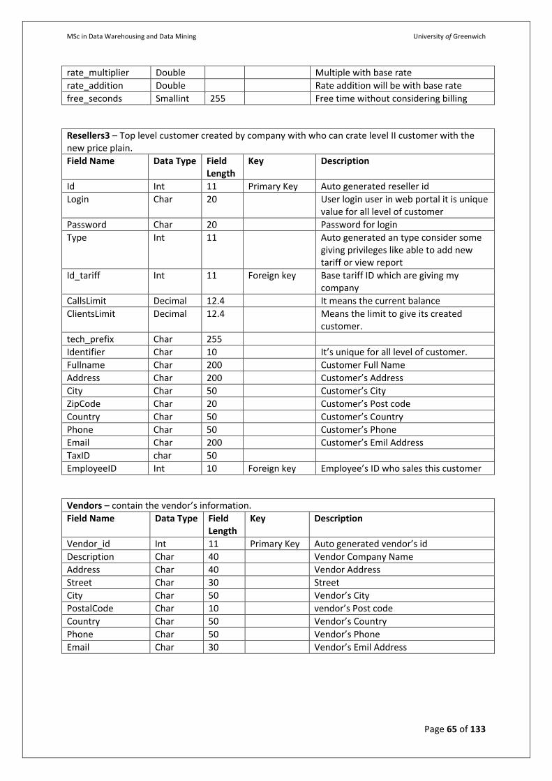
MSc in Data Warehousing and Data Mining University of Greenwich
Page 65 of 133
rate_multiplier Double Multiple with base rate
rate_addition Double Rate addition will be with base rate
free_seconds Smallint 255 Free time without considering billing
Resellers3 – Top level customer created by company with who can crate level II customer with the new price plain.
Field Name Data Type Field Length
Key Description
Id Int 11 Primary Key Auto generated reseller id
Login Char 20 User login user in web portal it is unique value for all level of customer
Password Char 20 Password for login
Type Int 11 Auto generated an type consider some giving privileges like able to add new tariff or view report
Id_tariff Int 11 Foreign key Base tariff ID which are giving my company
CallsLimit Decimal 12.4 It means the current balance
ClientsLimit Decimal 12.4 Means the limit to give its created customer.
tech_prefix Char 255
Identifier Char 10 It’s unique for all level of customer.
Fullname Char 200 Customer Full Name
Address Char 200 Customer’s Address
City Char 50 Customer’s City
ZipCode Char 20 Customer’s Post code
Country Char 50 Customer’s Country
Phone Char 50 Customer’s Phone
Email Char 200 Customer’s Emil Address
TaxID char 50
EmployeeID Int 10 Foreign key Employee’s ID who sales this customer
Vendors – contain the vendor’s information.
Field Name Data Type Field Length
Key Description
Vendor_id Int 11 Primary Key Auto generated vendor’s id
Description Char 40 Vendor Company Name
Address Char 40 Vendor Address
Street Char 30 Street
City Char 50 Vendor’s City
PostalCode Char 10 vendor’s Post code
Country Char 50 Vendor’s Country
Phone Char 50 Vendor’s Phone
Email Char 30 Vendor’s Emil Address
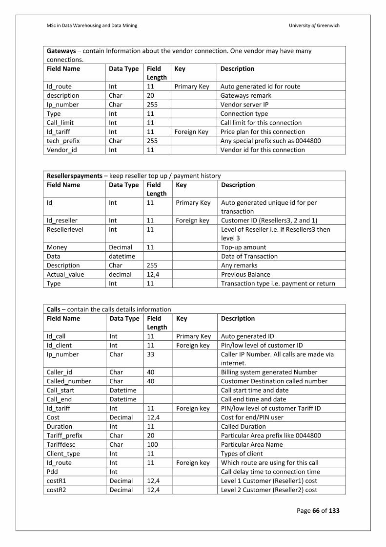
MSc in Data Warehousing and Data Mining University of Greenwich
Page 66 of 133
Gateways – contain Information about the vendor connection. One vendor may have many connections.
Field Name Data Type Field Length
Key Description
Id_route Int 11 Primary Key Auto generated id for route
description Char 20 Gateways remark
Ip_number Char 255 Vendor server IP
Type Int 11 Connection type
Call_limit Int 11 Call limit for this connection
Id_tariff Int 11 Foreign Key Price plan for this connection
tech_prefix Char 255 Any special prefix such as 0044800
Vendor_id Int 11 Vendor id for this connection
Resellerspayments – keep reseller top up / payment history
Field Name Data Type Field Length
Key Description
Id Int 11 Primary Key Auto generated unique id for per transaction
Id_reseller Int 11 Foreign key Customer ID (Resellers3, 2 and 1)
Resellerlevel Int 11 Level of Reseller i.e. if Resellers3 then level 3
Money Decimal 11 Top-up amount
Data datetime Data of Transaction
Description Char 255 Any remarks
Actual_value decimal 12,4 Previous Balance
Type Int 11 Transaction type i.e. payment or return
Calls – contain the calls details information
Field Name Data Type Field Length
Key Description
Id_call Int 11 Primary Key Auto generated ID
Id_client Int 11 Foreign key Pin/low level of customer ID
Ip_number Char 33 Caller IP Number. All calls are made via internet.
Caller_id Char 40 Billing system generated Number
Called_number Char 40 Customer Destination called number
Call_start Datetime Call start time and date
Call_end Datetime Call end time and date
Id_tariff Int 11 Foreign key PIN/low level of customer Tariff ID
Cost Decimal 12,4 Cost for end/PIN user
Duration Int 11 Called Duration
Tariff_prefix Char 20 Particular Area prefix like 0044800
Tariffdesc Char 100 Particular Area Name
Client_type Int 11 Types of client
Id_route Int 11 Foreign key Which route are using for this call
Pdd Int Call delay time to connection time
costR1 Decimal 12,4 Level 1 Customer (Reseller1) cost
costR2 Decimal 12,4 Level 2 Customer (Reseller2) cost

MSc in Data Warehousing and Data Mining University of Greenwich
Page 67 of 133
costR3 Decimal 12,4 Level 3 Customer (Reseller3) cost
CostD Decimal 12,4 Vendor Cost (optional if use tariff for vendor)
Id_reseller Int 11 Foreign key Level 1 Customer (Resellers1 ID)
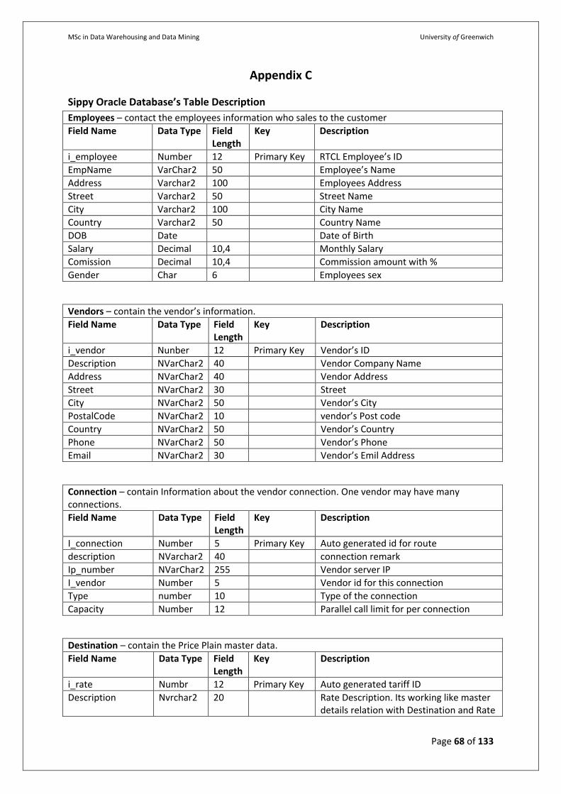
MSc in Data Warehousing and Data Mining University of Greenwich
Page 68 of 133
Appendix C
Sippy Oracle Database’s Table Description
Employees – contact the employees information who sales to the customer
Field Name Data Type Field Length
Key Description
i_employee Number 12 Primary Key RTCL Employee’s ID
EmpName VarChar2 50 Employee’s Name
Address Varchar2 100 Employees Address
Street Varchar2 50 Street Name
City Varchar2 100 City Name
Country Varchar2 50 Country Name
DOB Date Date of Birth
Salary Decimal 10,4 Monthly Salary
Comission Decimal 10,4 Commission amount with %
Gender Char 6 Employees sex
Vendors – contain the vendor’s information.
Field Name Data Type Field Length
Key Description
i_vendor Nunber 12 Primary Key Vendor’s ID
Description NVarChar2 40 Vendor Company Name
Address NVarChar2 40 Vendor Address
Street NVarChar2 30 Street
City NVarChar2 50 Vendor’s City
PostalCode NVarChar2 10 vendor’s Post code
Country NVarChar2 50 Vendor’s Country
Phone NVarChar2 50 Vendor’s Phone
Email NVarChar2 30 Vendor’s Emil Address
Connection – contain Information about the vendor connection. One vendor may have many connections.
Field Name Data Type Field Length
Key Description
I_connection Number 5 Primary Key Auto generated id for route
description NVarchar2 40 connection remark
Ip_number NVarChar2 255 Vendor server IP
I_vendor Number 5 Vendor id for this connection
Type number 10 Type of the connection
Capacity Number 12 Parallel call limit for per connection
Destination – contain the Price Plain master data.
Field Name Data Type Field Length
Key Description
i_rate Numbr 12 Primary Key Auto generated tariff ID
Description Nvrchar2 20 Rate Description. Its working like master details relation with Destination and Rate
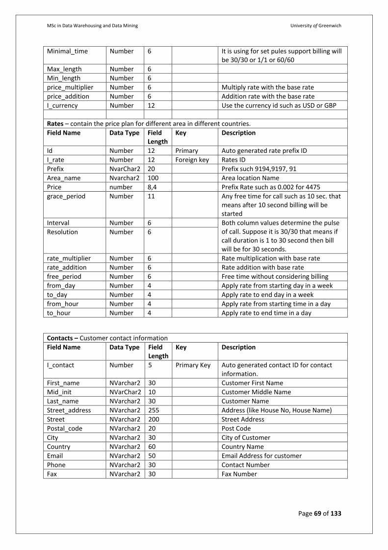
MSc in Data Warehousing and Data Mining University of Greenwich
Page 69 of 133
Minimal_time Number 6 It is using for set pules support billing will be 30/30 or 1/1 or 60/60
Max_length Number 6
Min_length Number 6
price_multiplier Number 6 Multiply rate with the base rate
price_addition Number 6 Addition rate with the base rate
I_currency Number 12 Use the currency id such as USD or GBP
Rates – contain the price plan for different area in different countries.
Field Name Data Type Field Length
Key Description
Id Number 12 Primary Auto generated rate prefix ID
I_rate Number 12 Foreign key Rates ID
Prefix NvarChar2 20 Prefix such 9194,9197, 91
Area_name Nvarchar2 100 Area location Name
Price number 8,4 Prefix Rate such as 0.002 for 4475
grace_period Number 11 Any free time for call such as 10 sec. that means after 10 second billing will be started
Interval Number 6 Both column values determine the pulse of call. Suppose it is 30/30 that means if call duration is 1 to 30 second then bill will be for 30 seconds.
Resolution Number 6
rate_multiplier Number 6 Rate multiplication with base rate
rate_addition Number 6 Rate addition with base rate
free_period Number 6 Free time without considering billing
from_day Number 4 Apply rate from starting day in a week
to_day Number 4 Apply rate to end day in a week
from_hour Number 4 Apply rate from starting time in a day
to_hour Number 4 Apply rate to end time in a day
Contacts – Customer contact information
Field Name Data Type Field Length
Key Description
I_contact Number 5 Primary Key Auto generated contact ID for contact information.
First_name NVarchar2 30 Customer First Name
Mid_init NVarChar2 10 Customer Middle Name
Last_name NVarchar2 30 Customer Name
Street_address NVarchar2 255 Address (like House No, House Name)
Street NVarchar2 200 Street Address
Postal_code NVarchar2 20 Post Code
City NVarchar2 30 City of Customer
Country NVarchar2 60 Country Name
Email NVarchar2 50 Email Address for customer
Phone NVarchar2 30 Contact Number
Fax NVarchar2 30 Fax Number
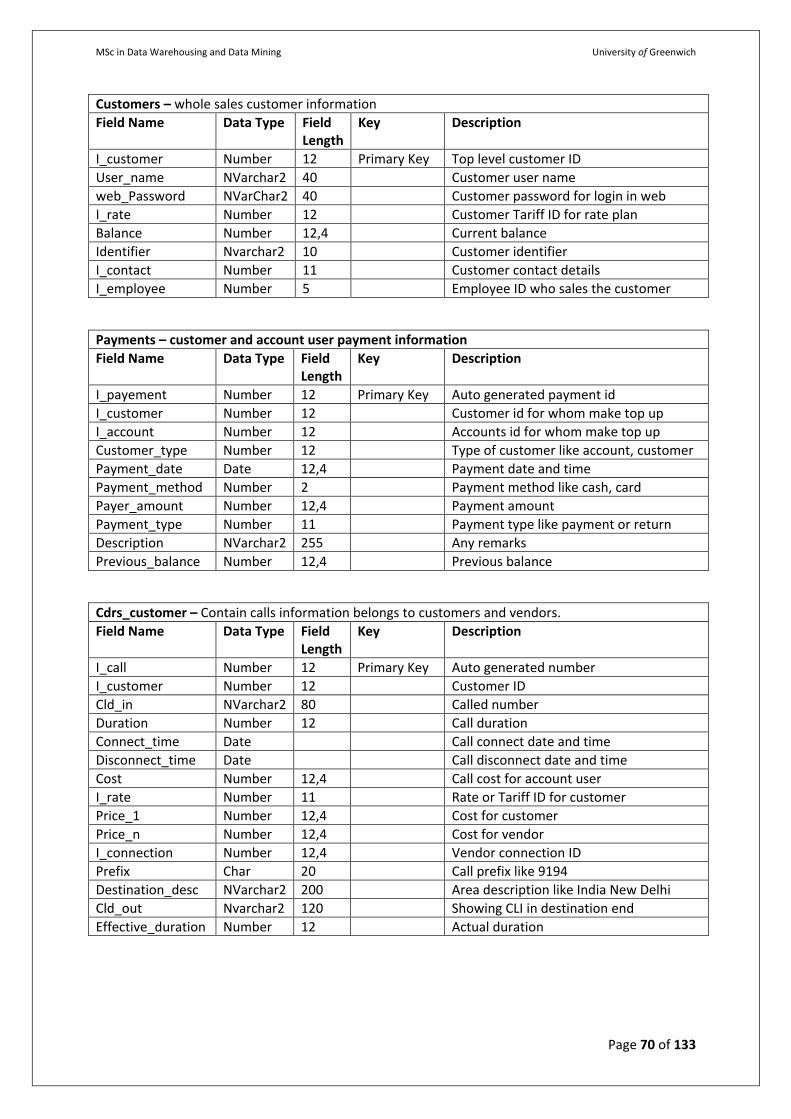
MSc in Data Warehousing and Data Mining University of Greenwich
Page 70 of 133
Customers – whole sales customer information
Field Name Data Type Field Length
Key Description
I_customer Number 12 Primary Key Top level customer ID
User_name NVarchar2 40 Customer user name
web_Password NVarChar2 40 Customer password for login in web
I_rate Number 12 Customer Tariff ID for rate plan
Balance Number 12,4 Current balance
Identifier Nvarchar2 10 Customer identifier
I_contact Number 11 Customer contact details
I_employee Number 5 Employee ID who sales the customer
Payments – customer and account user payment information
Field Name Data Type Field Length
Key Description
I_payement Number 12 Primary Key Auto generated payment id
I_customer Number 12 Customer id for whom make top up
I_account Number 12 Accounts id for whom make top up
Customer_type Number 12 Type of customer like account, customer
Payment_date Date 12,4 Payment date and time
Payment_method Number 2 Payment method like cash, card
Payer_amount Number 12,4 Payment amount
Payment_type Number 11 Payment type like payment or return
Description NVarchar2 255 Any remarks
Previous_balance Number 12,4 Previous balance
Cdrs_customer – Contain calls information belongs to customers and vendors.
Field Name Data Type Field Length
Key Description
I_call Number 12 Primary Key Auto generated number
I_customer Number 12 Customer ID
Cld_in NVarchar2 80 Called number
Duration Number 12 Call duration
Connect_time Date Call connect date and time
Disconnect_time Date Call disconnect date and time
Cost Number 12,4 Call cost for account user
I_rate Number 11 Rate or Tariff ID for customer
Price_1 Number 12,4 Cost for customer
Price_n Number 12,4 Cost for vendor
I_connection Number 12,4 Vendor connection ID
Prefix Char 20 Call prefix like 9194
Destination_desc NVarchar2 200 Area description like India New Delhi
Cld_out Nvarchar2 120 Showing CLI in destination end
Effective_duration Number 12 Actual duration
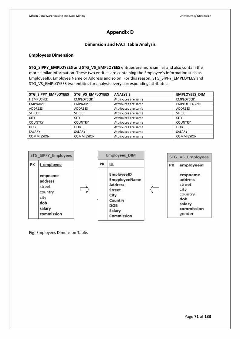
MSc in Data Warehousing and Data Mining University of Greenwich
Page 71 of 133
Appendix D
Dimension and FACT Table Analysis
Employees Dimension
STG_SIPPY_EMPLOYEES and STG_VS_EMPLOYEES entities are more similar and also contain the more similar information. These two entities are containing the Employee’s information such as EmployeeID, Employee Name or Address and so on. For this reason, STG_SIPPY_EMPLOYEES and STG_VS_EMPLOYEES two entities for analysis every corresponding attributes. STG_SIPPY_EMPLOYEES STG_VS_EMPLOYEES ANALYSIS EMPLOYEES_DIM I_EMPLOYEE EMPLOYEEID Attributes are same EMPLOYEEID
EMPNAME EMPNAME Attributes are same EMPLOYEENAME
ADDRESS ADDRESS Attributes are same ADDRESS
STREET STREET Attributes are same STREET
CITY CITY Attributes are same CITY
COUNTRY COUNTRY Attributes are same COUNTRY
DOB DOB Attributes are same DOB
SALARY SALARY Attributes are same SALARY
COMMISSION COMMISSION Attributes are same COMMISSION
Fig: Employees Dimension Table.
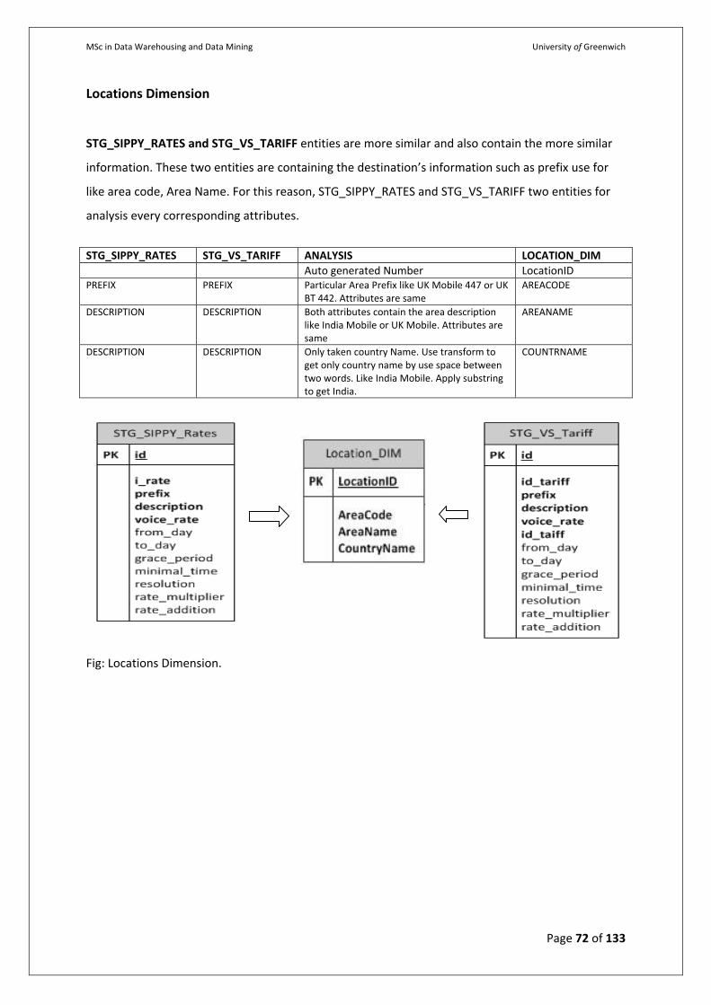
MSc in Data Warehousing and Data Mining University of Greenwich
Page 72 of 133
Locations Dimension
STG_SIPPY_RATES and STG_VS_TARIFF entities are more similar and also contain the more similar
information. These two entities are containing the destination’s information such as prefix use for
like area code, Area Name. For this reason, STG_SIPPY_RATES and STG_VS_TARIFF two entities for
analysis every corresponding attributes.
STG_SIPPY_RATES STG_VS_TARIFF ANALYSIS LOCATION_DIM
Auto generated Number LocationID PREFIX PREFIX Particular Area Prefix like UK Mobile 447 or UK
BT 442. Attributes are same AREACODE
DESCRIPTION DESCRIPTION Both attributes contain the area description like India Mobile or UK Mobile. Attributes are same
AREANAME
DESCRIPTION DESCRIPTION Only taken country Name. Use transform to get only country name by use space between two words. Like India Mobile. Apply substring to get India.
COUNTRNAME
Fig: Locations Dimension.
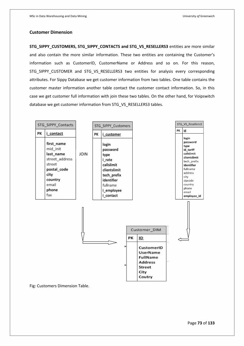
MSc in Data Warehousing and Data Mining University of Greenwich
Page 73 of 133
Customer Dimension
STG_SIPPY_CUSTOMERS, STG_SIPPY_CONTACTS and STG_VS_RESELLERS3 entities are more similar
and also contain the more similar information. These two entities are containing the Customer’s
information such as CustomerID, CustomerName or Address and so on. For this reason,
STG_SIPPY_CUSTOMER and STG_VS_RESELLERS3 two entities for analysis every corresponding
attributes. For Sippy Database we get customer information from two tables. One table contains the
customer master information another table contact the customer contact information. So, in this
case we get customer full information with join these two tables. On the other hand, for Voipswitch
database we get customer information from STG_VS_RESELLERS3 tables.
Fig: Customers Dimension Table.
JOIN
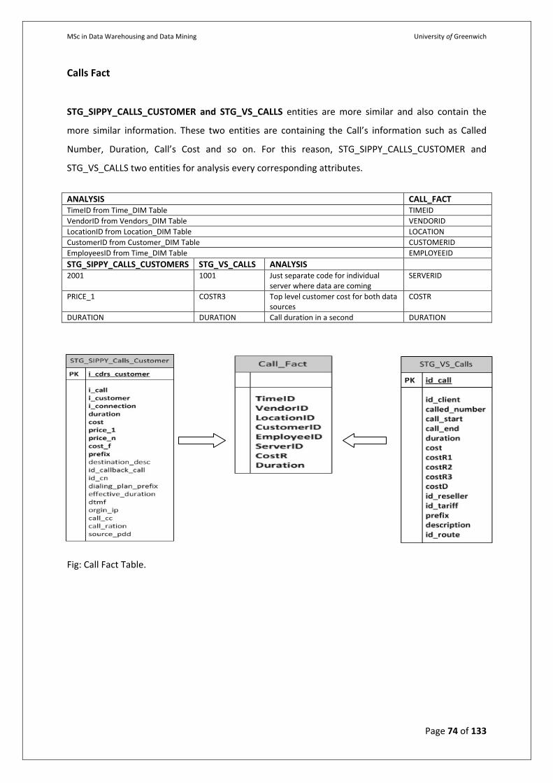
MSc in Data Warehousing and Data Mining University of Greenwich
Page 74 of 133
Calls Fact
STG_SIPPY_CALLS_CUSTOMER and STG_VS_CALLS entities are more similar and also contain the
more similar information. These two entities are containing the Call’s information such as Called
Number, Duration, Call’s Cost and so on. For this reason, STG_SIPPY_CALLS_CUSTOMER and
STG_VS_CALLS two entities for analysis every corresponding attributes.
ANALYSIS CALL_FACT TimeID from Time_DIM Table TIMEID
VendorID from Vendors_DIM Table VENDORID
LocationID from Location_DIM Table LOCATION
CustomerID from Customer_DIM Table CUSTOMERID
EmployeesID from Time_DIM Table EMPLOYEEID
STG_SIPPY_CALLS_CUSTOMERS STG_VS_CALLS ANALYSIS 2001 1001 Just separate code for individual
server where data are coming SERVERID
PRICE_1 COSTR3 Top level customer cost for both data sources
COSTR
DURATION DURATION Call duration in a second DURATION
Fig: Call Fact Table.
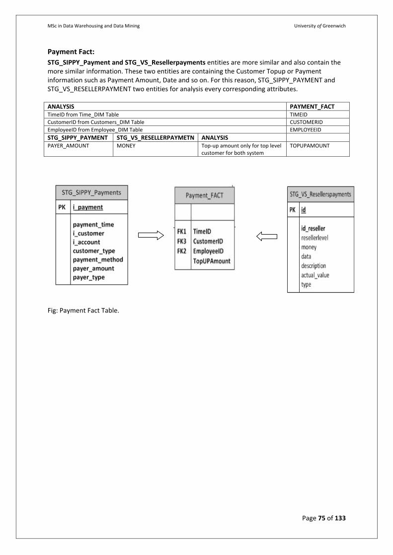
MSc in Data Warehousing and Data Mining University of Greenwich
Page 75 of 133
Payment Fact:
STG_SIPPY_Payment and STG_VS_Resellerpayments entities are more similar and also contain the more similar information. These two entities are containing the Customer Topup or Payment information such as Payment Amount, Date and so on. For this reason, STG_SIPPY_PAYMENT and STG_VS_RESELLERPAYMENT two entities for analysis every corresponding attributes. ANALYSIS PAYMENT_FACT TimeID from Time_DIM Table TIMEID
CustomerID from Customers_DIM Table CUSTOMERID
EmployeeID from Employee_DIM Table EMPLOYEEID
STG_SIPPY_PAYMENT STG_VS_RESELLERPAYMETN ANALYSIS
PAYER_AMOUNT MONEY Top-up amount only for top level customer for both system
TOPUPAMOUNT
Fig: Payment Fact Table.
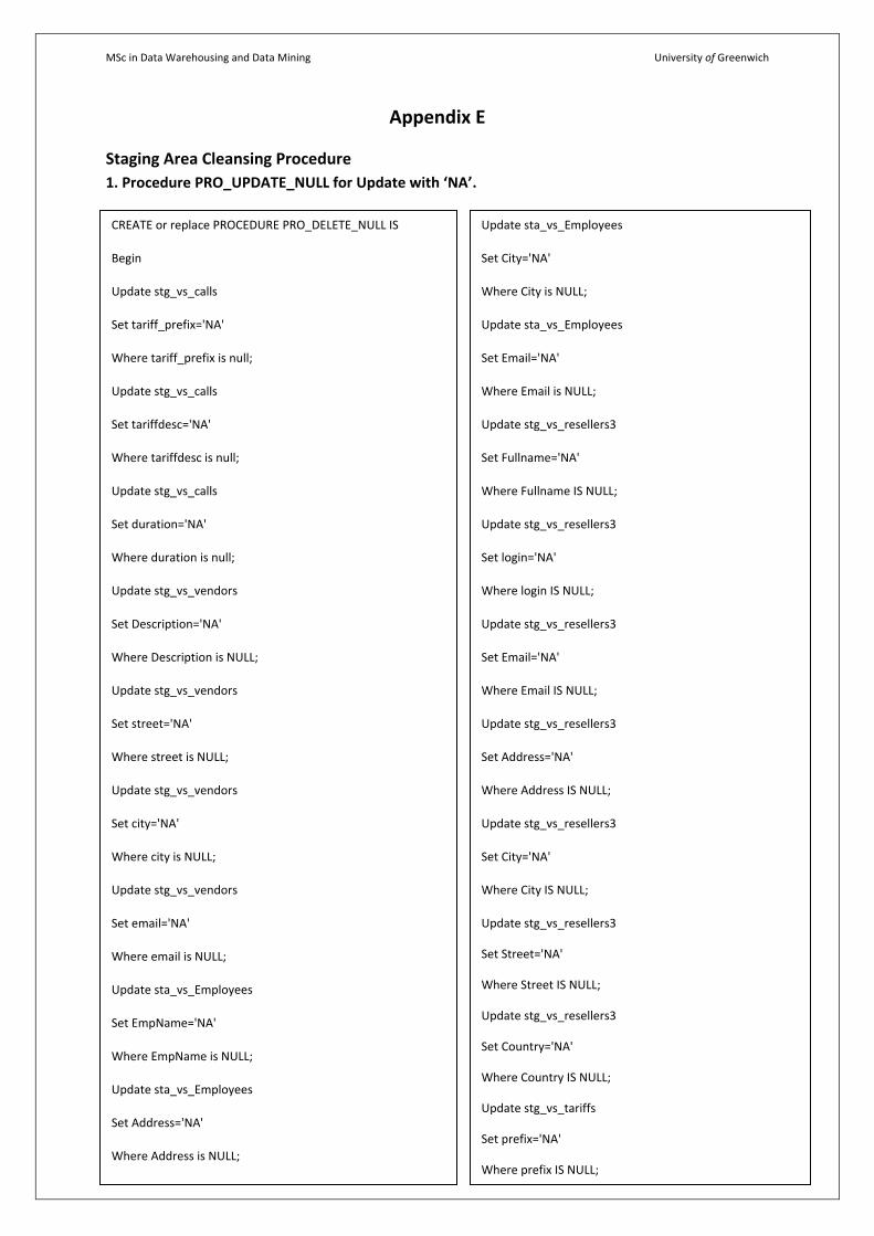
MSc in Data Warehousing and Data Mining University of Greenwich
Page 76 of 133
Appendix E
Staging Area Cleansing Procedure
1. Procedure PRO_UPDATE_NULL for Update with ‘NA’.
CREATE or replace PROCEDURE PRO_DELETE_NULL IS
Begin
Update stg_vs_calls
Set tariff_prefix='NA'
Where tariff_prefix is null;
Update stg_vs_calls
Set tariffdesc='NA'
Where tariffdesc is null;
Update stg_vs_calls
Set duration='NA'
Where duration is null;
Update stg_vs_vendors
Set Description='NA'
Where Description is NULL;
Update stg_vs_vendors
Set street='NA'
Where street is NULL;
Update stg_vs_vendors
Set city='NA'
Where city is NULL;
Update stg_vs_vendors
Set email='NA'
Where email is NULL;
Update sta_vs_Employees
Set EmpName='NA'
Where EmpName is NULL;
Update sta_vs_Employees
Set Address='NA'
Where Address is NULL;
Update sta_vs_Employees
Set City='NA'
Where City is NULL;
Update sta_vs_Employees
Set Email='NA'
Where Email is NULL;
Update stg_vs_resellers3
Set Fullname='NA'
Where Fullname IS NULL;
Update stg_vs_resellers3
Set login='NA'
Where login IS NULL;
Update stg_vs_resellers3
Set Email='NA'
Where Email IS NULL;
Update stg_vs_resellers3
Set Address='NA'
Where Address IS NULL;
Update stg_vs_resellers3
Set City='NA'
Where City IS NULL;
Update stg_vs_resellers3
Set Street='NA'
Where Street IS NULL;
Update stg_vs_resellers3
Set Country='NA'
Where Country IS NULL;
Update stg_vs_tariffs
Set prefix='NA'
Where prefix IS NULL;
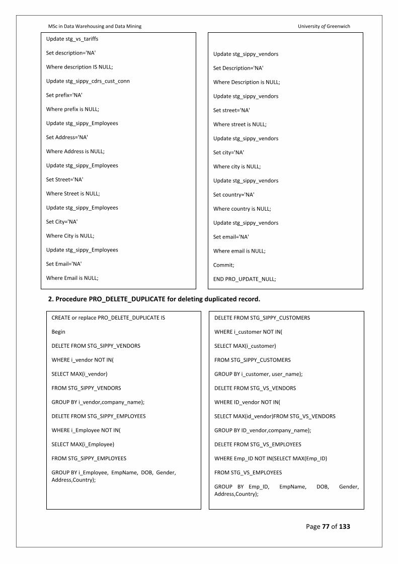
MSc in Data Warehousing and Data Mining University of Greenwich
Page 77 of 133
2. Procedure PRO_DELETE_DUPLICATE for deleting duplicated record.
DELETE FROM STG_VS_RESELLERS3
Update stg_vs_tariffs
Set description='NA'
Where description IS NULL;
Update stg_sippy_cdrs_cust_conn
Set prefix='NA'
Where prefix is NULL;
Update stg_sippy_Employees
Set Address='NA'
Where Address is NULL;
Update stg_sippy_Employees
Set Street='NA'
Where Street is NULL;
Update stg_sippy_Employees
Set City='NA'
Where City is NULL;
Update stg_sippy_Employees
Set Email='NA'
Where Email is NULL;
Update stg_sippy_vendors
Set Description='NA'
Where Description is NULL;
Update stg_sippy_vendors
Set street='NA'
Where street is NULL;
Update stg_sippy_vendors
Set city='NA'
Where city is NULL;
Update stg_sippy_vendors
Set country='NA'
Where country is NULL;
Update stg_sippy_vendors
Set email='NA'
Where email is NULL;
Commit;
END PRO_UPDATE_NULL;
CREATE or replace PRO_DELETE_DUPLICATE IS
Begin
DELETE FROM STG_SIPPY_VENDORS
WHERE i_vendor NOT IN(
SELECT MAX(i_vendor)
FROM STG_SIPPY_VENDORS
GROUP BY i_vendor,company_name);
DELETE FROM STG_SIPPY_EMPLOYEES
WHERE i_Employee NOT IN(
SELECT MAX(i_Employee)
FROM STG_SIPPY_EMPLOYEES
GROUP BY i_Employee, EmpName, DOB, Gender, Address,Country);
DELETE FROM STG_SIPPY_CUSTOMERS
WHERE i_customer NOT IN(
SELECT MAX(i_customer)
FROM STG_SIPPY_CUSTOMERS
GROUP BY i_customer, user_name);
DELETE FROM STG_VS_VENDORS
WHERE ID_vendor NOT IN(
SELECT MAX(id_vendor)FROM STG_VS_VENDORS
GROUP BY ID_vendor,company_name);
DELETE FROM STG_VS_EMPLOYEES
WHERE Emp_ID NOT IN(SELECT MAX(Emp_ID)
FROM STG_VS_EMPLOYEES
GROUP BY Emp_ID, EmpName, DOB, Gender, Address,Country);
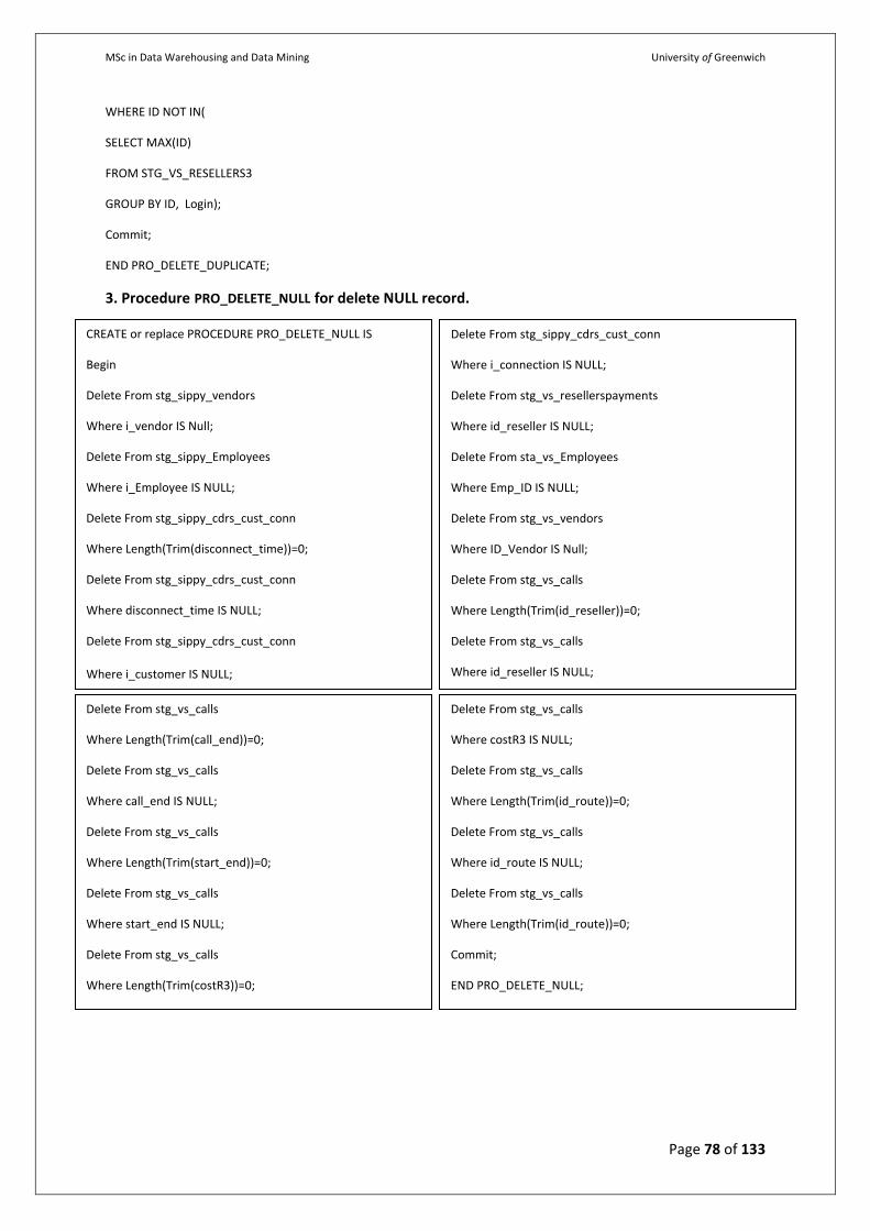
MSc in Data Warehousing and Data Mining University of Greenwich
Page 78 of 133
WHERE ID NOT IN(
SELECT MAX(ID)
FROM STG_VS_RESELLERS3
GROUP BY ID, Login);
Commit;
END PRO_DELETE_DUPLICATE;
3. Procedure PRO_DELETE_NULL for delete NULL record.
CREATE or replace PROCEDURE PRO_DELETE_NULL IS
Begin
Delete From stg_sippy_vendors
Where i_vendor IS Null;
Delete From stg_sippy_Employees
Where i_Employee IS NULL;
Delete From stg_sippy_cdrs_cust_conn
Where Length(Trim(disconnect_time))=0;
Delete From stg_sippy_cdrs_cust_conn
Where disconnect_time IS NULL;
Delete From stg_sippy_cdrs_cust_conn
Where i_customer IS NULL;
Delete From stg_sippy_cdrs_cust_conn
Where i_connection IS NULL;
Delete From stg_vs_resellerspayments
Where id_reseller IS NULL;
Delete From sta_vs_Employees
Where Emp_ID IS NULL;
Delete From stg_vs_vendors
Where ID_Vendor IS Null;
Delete From stg_vs_calls
Where Length(Trim(id_reseller))=0;
Delete From stg_vs_calls
Where id_reseller IS NULL;
Delete From stg_vs_calls
Where costR3 IS NULL;
Delete From stg_vs_calls
Where Length(Trim(id_route))=0;
Delete From stg_vs_calls
Where id_route IS NULL;
Delete From stg_vs_calls
Where Length(Trim(id_route))=0;
Commit;
END PRO_DELETE_NULL;
Delete From stg_vs_calls
Where Length(Trim(call_end))=0;
Delete From stg_vs_calls
Where call_end IS NULL;
Delete From stg_vs_calls
Where Length(Trim(start_end))=0;
Delete From stg_vs_calls
Where start_end IS NULL;
Delete From stg_vs_calls
Where Length(Trim(costR3))=0;
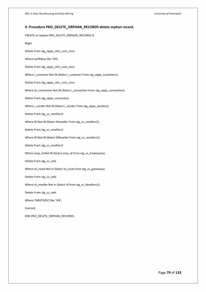
MSc in Data Warehousing and Data Mining University of Greenwich
Page 79 of 133
4. Procedure PRO_DELETE_ORPHAN_RECORDS delete orphan record.
CREATE or replace PRO_DELETE_ORPHAN_RECORDS IS
Begin
Delete From stg_sippy_cdrs_cust_conn
Where tariffdesc like ‘IVR’;
Delete From stg_sippy_cdrs_cust_conn
Where i_customer Not IN (Select i_customer From stg_sippy_customers);
Delete From stg_sippy_cdrs_cust_conn
Where id_connection Not IN (Select i_connection From stg_sippy_connection);
Delete From stg_sippy_connection
Where i_vendor Not IN (Select i_vendor From stg_sippy_vendors);
Delete From stg_vs_resellers3
Where ID Not IN (Select IDreseller From stg_vs_resellers2);
Delete From stg_vs_resellers2
Where ID Not IN (Select IDReseller From stg_vs_resellers1);
Delete From stg_vs_resellers3
Where emp_id Not IN (Select emp_id From stg_vs_Employees);
Delete From stg_vs_calls
Where id_route Not In (Select id_route from stg_vs_gateways);
Delete From stg_vs_calls
Where id_reseller Not In (Select id from stg_vs_Resellers1);
Delete From stg_vs_calls
Where TARIFFDESC like 'IVR';
Commit;
END PRO_DELETE_ORPHAN_RECORDS;
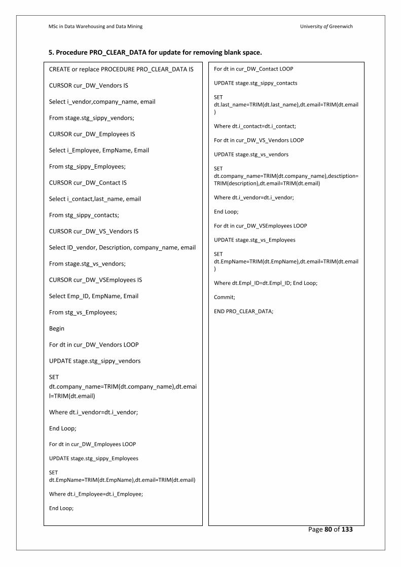
MSc in Data Warehousing and Data Mining University of Greenwich
Page 80 of 133
5. Procedure PRO_CLEAR_DATA for update for removing blank space.
CREATE or replace PROCEDURE PRO_CLEAR_DATA IS
CURSOR cur_DW_Vendors IS
Select i_vendor,company_name, email
From stage.stg_sippy_vendors;
CURSOR cur_DW_Employees IS
Select i_Employee, EmpName, Email
From stg_sippy_Employees;
CURSOR cur_DW_Contact IS
Select i_contact,last_name, email
From stg_sippy_contacts;
CURSOR cur_DW_VS_Vendors IS
Select ID_vendor, Description, company_name, email
From stage.stg_vs_vendors;
CURSOR cur_DW_VSEmployees IS
Select Emp_ID, EmpName, Email
From stg_vs_Employees;
Begin
For dt in cur_DW_Vendors LOOP
UPDATE stage.stg_sippy_vendors
SET
dt.company_name=TRIM(dt.company_name),dt.emai
l=TRIM(dt.email)
Where dt.i_vendor=dt.i_vendor;
End Loop;
For dt in cur_DW_Employees LOOP
UPDATE stage.stg_sippy_Employees
SET dt.EmpName=TRIM(dt.EmpName),dt.email=TRIM(dt.email)
Where dt.i_Employee=dt.i_Employee;
End Loop;
For dt in cur_DW_Contact LOOP
UPDATE stage.stg_sippy_contacts
SET dt.last_name=TRIM(dt.last_name),dt.email=TRIM(dt.email)
Where dt.i_contact=dt.i_contact;
For dt in cur_DW_VS_Vendors LOOP
UPDATE stage.stg_vs_vendors
SET dt.company_name=TRIM(dt.company_name),desctiption=TRIM(description),dt.email=TRIM(dt.email)
Where dt.i_vendor=dt.i_vendor;
End Loop;
For dt in cur_DW_VSEmployees LOOP
UPDATE stage.stg_vs_Employees
SET dt.EmpName=TRIM(dt.EmpName),dt.email=TRIM(dt.email)
Where dt.Empl_ID=dt.Empl_ID; End Loop;
Commit;
END PRO_CLEAR_DATA;
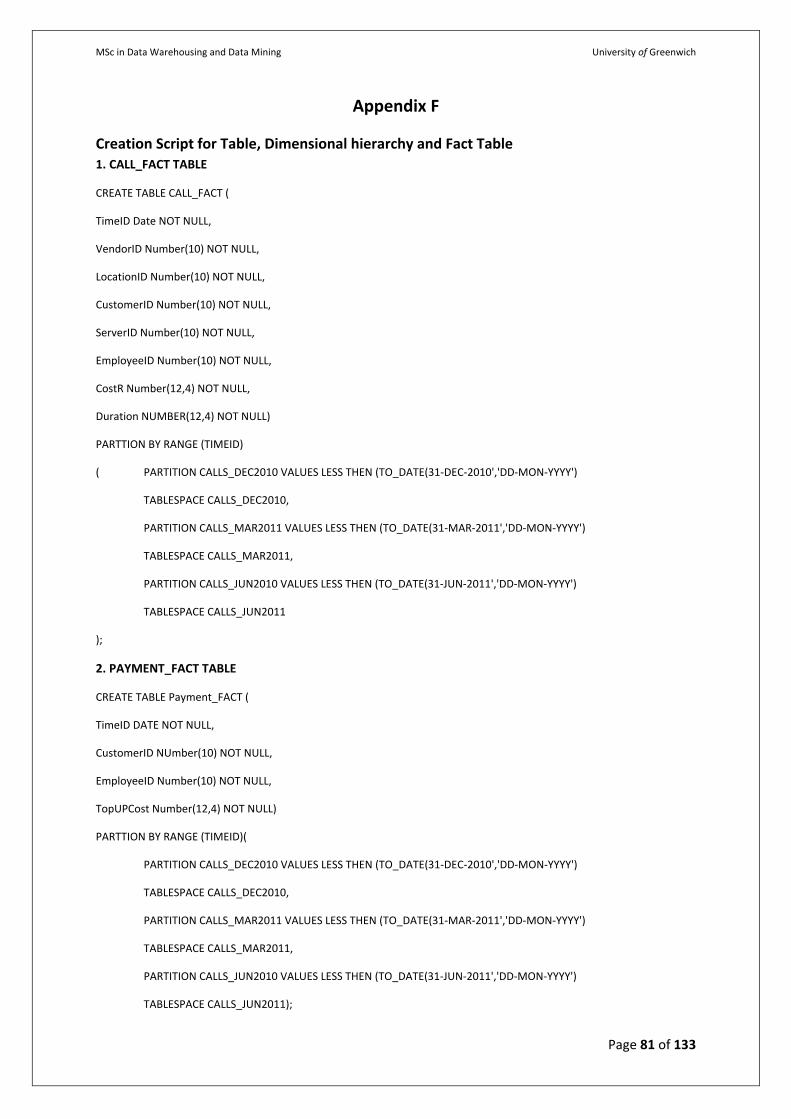
MSc in Data Warehousing and Data Mining University of Greenwich
Page 81 of 133
Appendix F
Creation Script for Table, Dimensional hierarchy and Fact Table 1. CALL_FACT TABLE
CREATE TABLE CALL_FACT (
TimeID Date NOT NULL,
VendorID Number(10) NOT NULL,
LocationID Number(10) NOT NULL,
CustomerID Number(10) NOT NULL,
ServerID Number(10) NOT NULL,
EmployeeID Number(10) NOT NULL,
CostR Number(12,4) NOT NULL,
Duration NUMBER(12,4) NOT NULL)
PARTTION BY RANGE (TIMEID)
( PARTITION CALLS_DEC2010 VALUES LESS THEN (TO_DATE(31-DEC-2010','DD-MON-YYYY')
TABLESPACE CALLS_DEC2010,
PARTITION CALLS_MAR2011 VALUES LESS THEN (TO_DATE(31-MAR-2011','DD-MON-YYYY')
TABLESPACE CALLS_MAR2011,
PARTITION CALLS_JUN2010 VALUES LESS THEN (TO_DATE(31-JUN-2011','DD-MON-YYYY')
TABLESPACE CALLS_JUN2011
);
2. PAYMENT_FACT TABLE
CREATE TABLE Payment_FACT (
TimeID DATE NOT NULL,
CustomerID NUmber(10) NOT NULL,
EmployeeID Number(10) NOT NULL,
TopUPCost Number(12,4) NOT NULL)
PARTTION BY RANGE (TIMEID)(
PARTITION CALLS_DEC2010 VALUES LESS THEN (TO_DATE(31-DEC-2010','DD-MON-YYYY')
TABLESPACE CALLS_DEC2010,
PARTITION CALLS_MAR2011 VALUES LESS THEN (TO_DATE(31-MAR-2011','DD-MON-YYYY')
TABLESPACE CALLS_MAR2011,
PARTITION CALLS_JUN2010 VALUES LESS THEN (TO_DATE(31-JUN-2011','DD-MON-YYYY')
TABLESPACE CALLS_JUN2011);
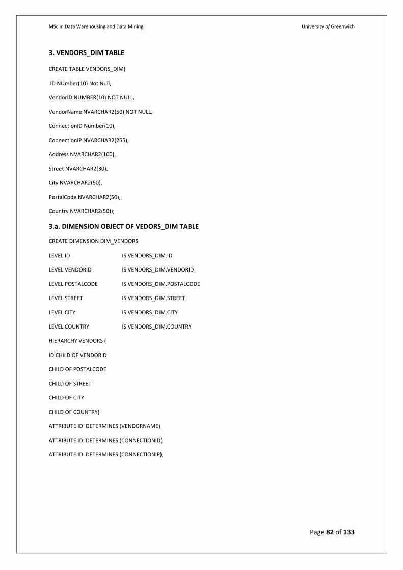
MSc in Data Warehousing and Data Mining University of Greenwich
Page 82 of 133
3. VENDORS_DIM TABLE
CREATE TABLE VENDORS_DIM(
ID NUmber(10) Not Null,
VendorID NUMBER(10) NOT NULL,
VendorName NVARCHAR2(50) NOT NULL,
ConnectionID Number(10),
ConnectionIP NVARCHAR2(255),
Address NVARCHAR2(100),
Street NVARCHAR2(30),
City NVARCHAR2(50),
PostalCode NVARCHAR2(50),
Country NVARCHAR2(50));
3.a. DIMENSION OBJECT OF VEDORS_DIM TABLE
CREATE DIMENSION DIM_VENDORS
LEVEL ID IS VENDORS_DIM.ID
LEVEL VENDORID IS VENDORS_DIM.VENDORID
LEVEL POSTALCODE IS VENDORS_DIM.POSTALCODE
LEVEL STREET IS VENDORS_DIM.STREET
LEVEL CITY IS VENDORS_DIM.CITY
LEVEL COUNTRY IS VENDORS_DIM.COUNTRY
HIERARCHY VENDORS (
ID CHILD OF VENDORID
CHILD OF POSTALCODE
CHILD OF STREET
CHILD OF CITY
CHILD OF COUNTRY)
ATTRIBUTE ID DETERMINES (VENDORNAME)
ATTRIBUTE ID DETERMINES (CONNECTIONID)
ATTRIBUTE ID DETERMINES (CONNECTIONIP);
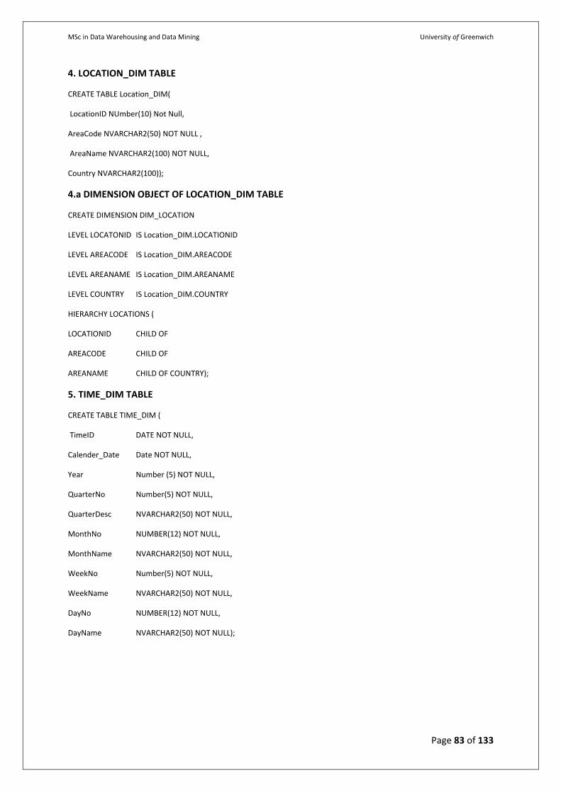
MSc in Data Warehousing and Data Mining University of Greenwich
Page 83 of 133
4. LOCATION_DIM TABLE
CREATE TABLE Location_DIM(
LocationID NUmber(10) Not Null,
AreaCode NVARCHAR2(50) NOT NULL ,
AreaName NVARCHAR2(100) NOT NULL,
Country NVARCHAR2(100));
4.a DIMENSION OBJECT OF LOCATION_DIM TABLE
CREATE DIMENSION DIM_LOCATION
LEVEL LOCATONID IS Location_DIM.LOCATIONID
LEVEL AREACODE IS Location_DIM.AREACODE
LEVEL AREANAME IS Location_DIM.AREANAME
LEVEL COUNTRY IS Location_DIM.COUNTRY
HIERARCHY LOCATIONS (
LOCATIONID CHILD OF
AREACODE CHILD OF
AREANAME CHILD OF COUNTRY);
5. TIME_DIM TABLE
CREATE TABLE TIME_DIM (
TimeID DATE NOT NULL,
Calender_Date Date NOT NULL,
Year Number (5) NOT NULL,
QuarterNo Number(5) NOT NULL,
QuarterDesc NVARCHAR2(50) NOT NULL,
MonthNo NUMBER(12) NOT NULL,
MonthName NVARCHAR2(50) NOT NULL,
WeekNo Number(5) NOT NULL,
WeekName NVARCHAR2(50) NOT NULL,
DayNo NUMBER(12) NOT NULL,
DayName NVARCHAR2(50) NOT NULL);
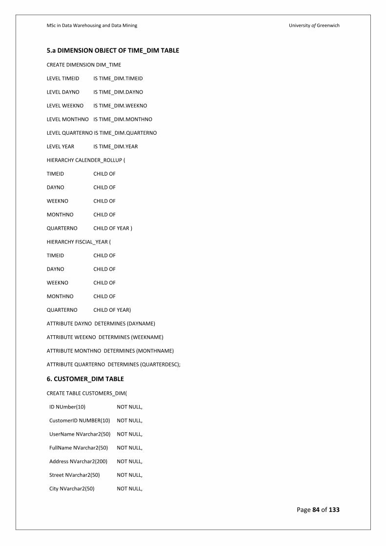
MSc in Data Warehousing and Data Mining University of Greenwich
Page 84 of 133
5.a DIMENSION OBJECT OF TIME_DIM TABLE
CREATE DIMENSION DIM_TIME
LEVEL TIMEID IS TIME_DIM.TIMEID
LEVEL DAYNO IS TIME_DIM.DAYNO
LEVEL WEEKNO IS TIME_DIM.WEEKNO
LEVEL MONTHNO IS TIME_DIM.MONTHNO
LEVEL QUARTERNO IS TIME_DIM.QUARTERNO
LEVEL YEAR IS TIME_DIM.YEAR
HIERARCHY CALENDER_ROLLUP (
TIMEID CHILD OF
DAYNO CHILD OF
WEEKNO CHILD OF
MONTHNO CHILD OF
QUARTERNO CHILD OF YEAR )
HIERARCHY FISCIAL_YEAR (
TIMEID CHILD OF
DAYNO CHILD OF
WEEKNO CHILD OF
MONTHNO CHILD OF
QUARTERNO CHILD OF YEAR)
ATTRIBUTE DAYNO DETERMINES (DAYNAME)
ATTRIBUTE WEEKNO DETERMINES (WEEKNAME)
ATTRIBUTE MONTHNO DETERMINES (MONTHNAME)
ATTRIBUTE QUARTERNO DETERMINES (QUARTERDESC);
6. CUSTOMER_DIM TABLE
CREATE TABLE CUSTOMERS_DIM(
ID NUmber(10) NOT NULL,
CustomerID NUMBER(10) NOT NULL,
UserName NVarchar2(50) NOT NULL,
FullName NVarchar2(50) NOT NULL,
Address NVarchar2(200) NOT NULL,
Street NVarchar2(50) NOT NULL,
City NVarchar2(50) NOT NULL,

MSc in Data Warehousing and Data Mining University of Greenwich
Page 85 of 133
Country NVarchar2(50) NOT NULL,
Phone NVarchar2(50) NOT NULL,
Email NVarchar2(50) NOT NULL,
CustomerMGRID NUMBER(10,0) DEFAULT '0' NOT NULL,
CustomerLevelID NUMBER(10,0) DEFAULT '0' NOT NULL,
ServerID Number(5) NOT NULL);
6.a DIMENSION OBJECT OF CUSTOMER_DIM TABLE
CREATE DIMENSION DIM_CUSTOMERS
LEVEL ID IS CUSTOMERS_DIM.ID
LEVEL CUSTOMERID IS CUSTOMERS_DIM.VENDORID
LEVEL STREET IS CUSTOMERS_DIM.STREET
LEVEL CITY IS CUSTOMERS_DIM.CITY
LEVEL COUNTRY IS CUSTOMERS_DIM.COUNTRY
HIERARCHY ROLL_UP
(
ID CHILD OF
CUSTOMERID CHILD OF
STREET CHILD OF
CITY CHILD OF
COUNTRY
)
ATTRIBUTE ID DETERMINES (USERNAME)
ATTRIBUTE ID DETERMINES (FULLNAME)
ATTRIBUTE ID DETERMINES (ADDRESS)
ATTRIBUTE ID DETERMINES (PHONE)
ATTRIBUTE ID DETERMINES (EMAIL)
ATTRIBUTE ID DETERMINES (CUSTOMERMEGID)
ATTRIBUTE ID DETERMINES (CUSTOMERLEVELID)
ATTRIBUTE ID DETERMINES (SERVERID);
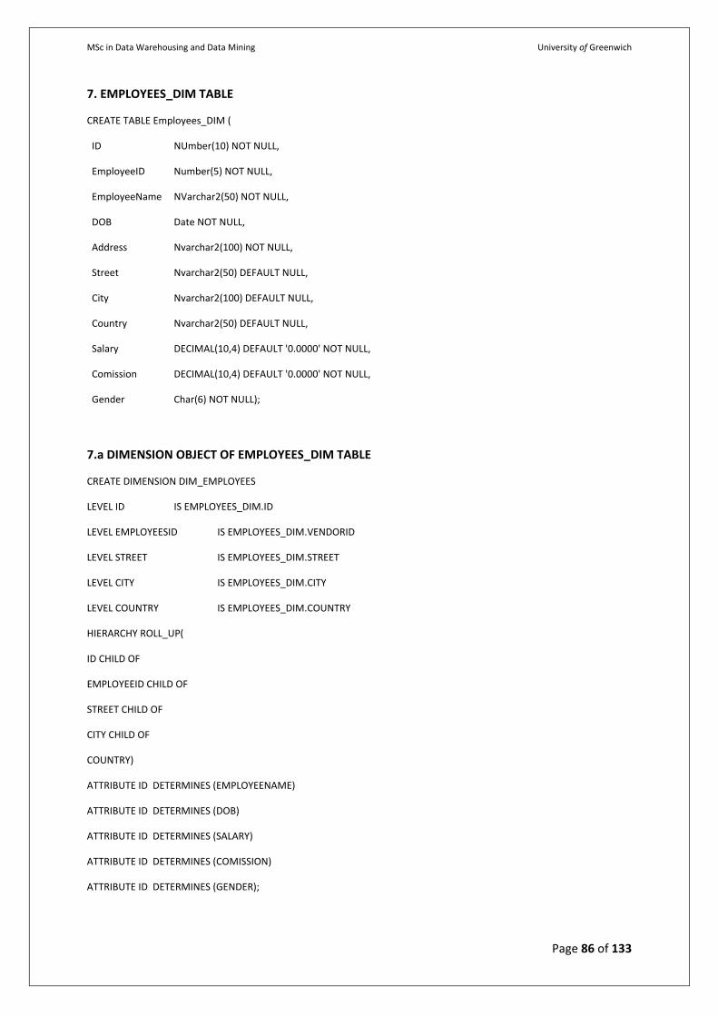
MSc in Data Warehousing and Data Mining University of Greenwich
Page 86 of 133
7. EMPLOYEES_DIM TABLE
CREATE TABLE Employees_DIM (
ID NUmber(10) NOT NULL,
EmployeeID Number(5) NOT NULL,
EmployeeName NVarchar2(50) NOT NULL,
DOB Date NOT NULL,
Address Nvarchar2(100) NOT NULL,
Street Nvarchar2(50) DEFAULT NULL,
City Nvarchar2(100) DEFAULT NULL,
Country Nvarchar2(50) DEFAULT NULL,
Salary DECIMAL(10,4) DEFAULT '0.0000' NOT NULL,
Comission DECIMAL(10,4) DEFAULT '0.0000' NOT NULL,
Gender Char(6) NOT NULL);
7.a DIMENSION OBJECT OF EMPLOYEES_DIM TABLE
CREATE DIMENSION DIM_EMPLOYEES
LEVEL ID IS EMPLOYEES_DIM.ID
LEVEL EMPLOYEESID IS EMPLOYEES_DIM.VENDORID
LEVEL STREET IS EMPLOYEES_DIM.STREET
LEVEL CITY IS EMPLOYEES_DIM.CITY
LEVEL COUNTRY IS EMPLOYEES_DIM.COUNTRY
HIERARCHY ROLL_UP(
ID CHILD OF
EMPLOYEEID CHILD OF
STREET CHILD OF
CITY CHILD OF
COUNTRY)
ATTRIBUTE ID DETERMINES (EMPLOYEENAME)
ATTRIBUTE ID DETERMINES (DOB)
ATTRIBUTE ID DETERMINES (SALARY)
ATTRIBUTE ID DETERMINES (COMISSION)
ATTRIBUTE ID DETERMINES (GENDER);
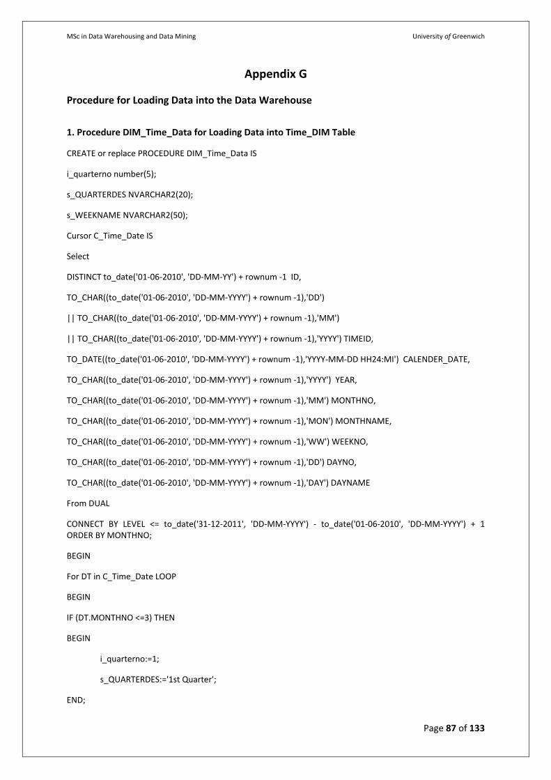
MSc in Data Warehousing and Data Mining University of Greenwich
Page 87 of 133
Appendix G
Procedure for Loading Data into the Data Warehouse
1. Procedure DIM_Time_Data for Loading Data into Time_DIM Table
CREATE or replace PROCEDURE DIM_Time_Data IS
i_quarterno number(5);
s_QUARTERDES NVARCHAR2(20);
s_WEEKNAME NVARCHAR2(50);
Cursor C_Time_Date IS
Select
DISTINCT to_date('01-06-2010', 'DD-MM-YY') + rownum -1 ID,
TO_CHAR((to_date('01-06-2010', 'DD-MM-YYYY') + rownum -1),'DD')
|| TO_CHAR((to_date('01-06-2010', 'DD-MM-YYYY') + rownum -1),'MM')
|| TO_CHAR((to_date('01-06-2010', 'DD-MM-YYYY') + rownum -1),'YYYY') TIMEID,
TO_DATE((to_date('01-06-2010', 'DD-MM-YYYY') + rownum -1),'YYYY-MM-DD HH24:MI') CALENDER_DATE,
TO_CHAR((to_date('01-06-2010', 'DD-MM-YYYY') + rownum -1),'YYYY') YEAR,
TO_CHAR((to_date('01-06-2010', 'DD-MM-YYYY') + rownum -1),'MM') MONTHNO,
TO_CHAR((to_date('01-06-2010', 'DD-MM-YYYY') + rownum -1),'MON') MONTHNAME,
TO_CHAR((to_date('01-06-2010', 'DD-MM-YYYY') + rownum -1),'WW') WEEKNO,
TO_CHAR((to_date('01-06-2010', 'DD-MM-YYYY') + rownum -1),'DD') DAYNO,
TO_CHAR((to_date('01-06-2010', 'DD-MM-YYYY') + rownum -1),'DAY') DAYNAME
From DUAL
CONNECT BY LEVEL <= to_date('31-12-2011', 'DD-MM-YYYY') - to_date('01-06-2010', 'DD-MM-YYYY') + 1 ORDER BY MONTHNO;
BEGIN
For DT in C_Time_Date LOOP
BEGIN
IF (DT.MONTHNO <=3) THEN
BEGIN
i_quarterno:=1;
s_QUARTERDES:='1st Quarter';
END;
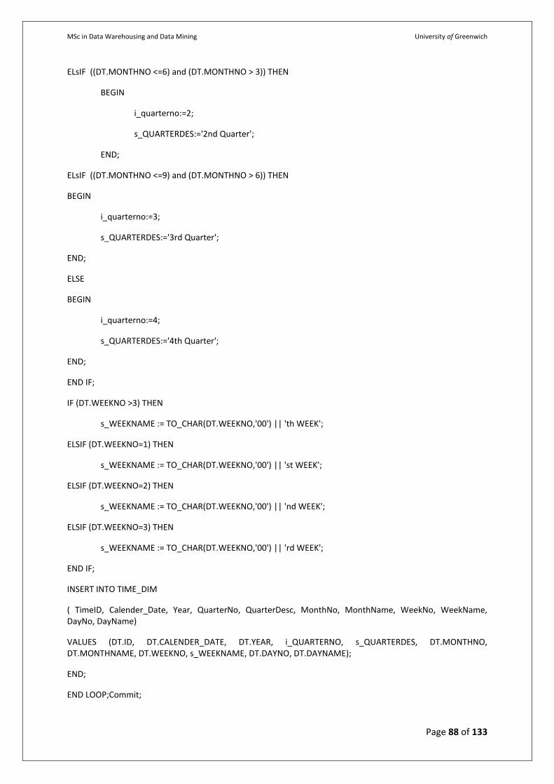
MSc in Data Warehousing and Data Mining University of Greenwich
Page 88 of 133
ELsIF ((DT.MONTHNO <=6) and (DT.MONTHNO > 3)) THEN
BEGIN
i_quarterno:=2;
s_QUARTERDES:='2nd Quarter';
END;
ELsIF ((DT.MONTHNO <=9) and (DT.MONTHNO > 6)) THEN
BEGIN
i_quarterno:=3;
s_QUARTERDES:='3rd Quarter';
END;
ELSE
BEGIN
i_quarterno:=4;
s_QUARTERDES:='4th Quarter';
END;
END IF;
IF (DT.WEEKNO >3) THEN
s_WEEKNAME := TO_CHAR(DT.WEEKNO,'00') || 'th WEEK';
ELSIF (DT.WEEKNO=1) THEN
s_WEEKNAME := TO_CHAR(DT.WEEKNO,'00') || 'st WEEK';
ELSIF (DT.WEEKNO=2) THEN
s_WEEKNAME := TO_CHAR(DT.WEEKNO,'00') || 'nd WEEK';
ELSIF (DT.WEEKNO=3) THEN
s_WEEKNAME := TO_CHAR(DT.WEEKNO,'00') || 'rd WEEK';
END IF;
INSERT INTO TIME_DIM
( TimeID, Calender_Date, Year, QuarterNo, QuarterDesc, MonthNo, MonthName, WeekNo, WeekName, DayNo, DayName)
VALUES (DT.ID, DT.CALENDER_DATE, DT.YEAR, i_QUARTERNO, s_QUARTERDES, DT.MONTHNO, DT.MONTHNAME, DT.WEEKNO, s_WEEKNAME, DT.DAYNO, DT.DAYNAME);
END;
END LOOP;Commit;
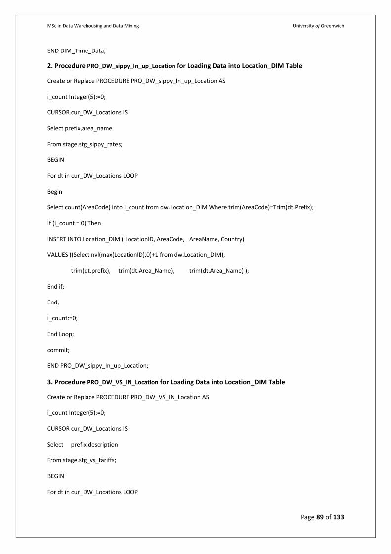
MSc in Data Warehousing and Data Mining University of Greenwich
Page 89 of 133
END DIM_Time_Data;
2. Procedure PRO_DW_sippy_In_up_Location for Loading Data into Location_DIM Table
Create or Replace PROCEDURE PRO_DW_sippy_In_up_Location AS
i_count Integer(5):=0;
CURSOR cur_DW_Locations IS
Select prefix,area_name
From stage.stg_sippy_rates;
BEGIN
For dt in cur_DW_Locations LOOP
Begin
Select count(AreaCode) into i_count from dw.Location_DIM Where trim(AreaCode)=Trim(dt.Prefix);
If (i_count = 0) Then
INSERT INTO Location_DIM ( LocationID, AreaCode, AreaName, Country)
VALUES ((Select nvl(max(LocationID),0)+1 from dw.Location_DIM),
trim(dt.prefix), trim(dt.Area_Name), trim(dt.Area_Name) );
End if;
End;
i_count:=0;
End Loop;
commit;
END PRO_DW_sippy_In_up_Location;
3. Procedure PRO_DW_VS_IN_Location for Loading Data into Location_DIM Table
Create or Replace PROCEDURE PRO_DW_VS_IN_Location AS
i_count Integer(5):=0;
CURSOR cur_DW_Locations IS
Select prefix,description
From stage.stg_vs_tariffs;
BEGIN
For dt in cur_DW_Locations LOOP
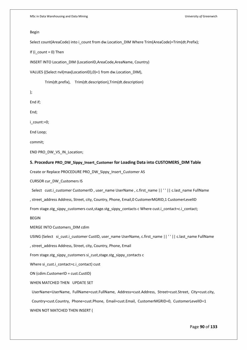
MSc in Data Warehousing and Data Mining University of Greenwich
Page 90 of 133
Begin
Select count(AreaCode) into i_count from dw.Location_DIM Where Trim(AreaCode)=Trim(dt.Prefix);
If (i_count = 0) Then
INSERT INTO Location_DIM (LocationID,AreaCode,AreaName, Country)
VALUES ((Select nvl(max(LocationID),0)+1 from dw.Location_DIM),
Trim(dt.prefix), Trim(dt.description),Trim(dt.description)
);
End if;
End;
i_count:=0;
End Loop;
commit;
END PRO_DW_VS_IN_Location;
5. Procedure PRO_DW_Sippy_Insert_Customer for Loading Data into CUSTOMERS_DIM Table
Create or Replace PROCEDURE PRO_DW_Sippy_Insert_Customer AS
CURSOR cur_DW_Customers IS
Select cust.i_customer CustomerID , user_name UserName , c.first_name || ' ' || c.last_name FullName
, street_address Address, Street, city, Country, Phone, Email,0 CustomerMGRID,1 CustomerLevelID
From stage.stg_sippy_customers cust,stage.stg_sippy_contacts c Where cust.i_contact=c.i_contact;
BEGIN
MERGE INTO Customers_DIM cdim
USING (Select si_cust.i_customer CustID, user_name UserName, c.first_name || ' ' || c.last_name FullName
, street_address Address, Street, city, Country, Phone, Email
From stage.stg_sippy_customers si_cust,stage.stg_sippy_contacts c
Where si_cust.i_contact=c.i_contact) cust
ON (cdim.CustomerID = cust.CustID)
WHEN MATCHED THEN UPDATE SET
UserName=UserName, FullName=cust.FullName, Address=cust.Address, Street=cust.Street, City=cust.city,
Country=cust.Country, Phone=cust.Phone, Email=cust.Email, CustomerMGRID=0, CustomerLevelID=1
WHEN NOT MATCHED THEN INSERT (
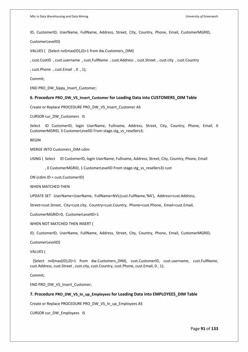
MSc in Data Warehousing and Data Mining University of Greenwich
Page 91 of 133
ID, CustomerID, UserName, FullName, Address, Street, City, Country, Phone, Email, CustomerMGRID,
CustomerLevelID)
VALUES ( (Select nvl(max(ID),0)+1 from dw.Customers_DIM)
, cust.CustID , cust.username , cust.FullName , cust.Address , cust.Street , cust.city , cust.Country
, cust.Phone , cust.Email , 0 , 1);
Commit;
END PRO_DW_Sippy_Insert_Customer;
6. Procedure PRO_DW_VS_Insert_Customer for Loading Data into CUSTOMERS_DIM Table
Create or Replace PROCEDURE PRO_DW_VS_Insert_Customer AS
CURSOR cur_DW_Customers IS
Select ID CustomerID, login UserName, Fullname, Address, Street, City, Country, Phone, Email, 0 CustomerMGRID, 3 CustomerLevelID From stage.stg_vs_resellers3;
BEGIN
MERGE INTO Customers_DIM cdim
USING ( Select ID CustomerID, login UserName, Fullname, Address, Street, City, Country, Phone, Email
, 0 CustomerMGRID, 1 CustomerLevelID From stage.stg_vs_resellers3) cust
ON (cdim.ID = cust.CustomerID)
WHEN MATCHED THEN
UPDATE SET UserName=UserName, FullName=NVL(cust.FullName,'NA'), Address=cust.Address,
Street=cust.Street, City=cust.city, Country=cust.Country, Phone=cust.Phone, Email=cust.Email,
CustomerMGRID=0, CustomerLevelID=1
WHEN NOT MATCHED THEN INSERT (
ID, CustomerID, UserName, FullName, Address, Street, City, Country, Phone, Email, CustomerMGRID,
CustomerLevelID)
VALUES (
(Select nvl(max(ID),0)+1 from dw.Customers_DIM), cust.CustomerID, cust.username, cust.FullName, cust.Address, cust.Street , cust.city, cust.Country, cust.Phone, cust.Email, 0 , 1);
Commit;
END PRO_DW_VS_Insert_Customer;
7. Procedure PRO_DW_VS_In_up_Employees for Loading Data into EMPLOYEES_DIM Table
Create or Replace PROCEDURE PRO_DW_VS_In_up_Employees AS
CURSOR cur_DW_Employees IS
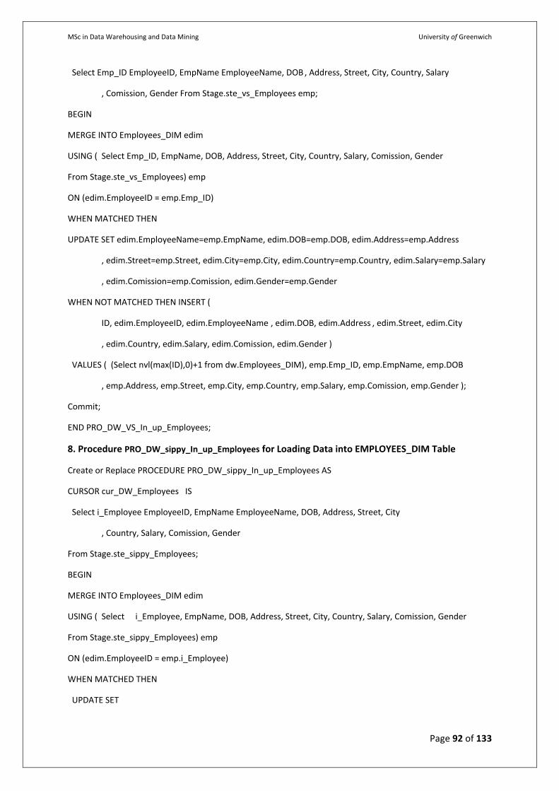
MSc in Data Warehousing and Data Mining University of Greenwich
Page 92 of 133
Select Emp_ID EmployeeID, EmpName EmployeeName, DOB , Address, Street, City, Country, Salary
, Comission, Gender From Stage.ste_vs_Employees emp;
BEGIN
MERGE INTO Employees_DIM edim
USING ( Select Emp_ID, EmpName, DOB, Address, Street, City, Country, Salary, Comission, Gender
From Stage.ste_vs_Employees) emp
ON (edim.EmployeeID = emp.Emp_ID)
WHEN MATCHED THEN
UPDATE SET edim.EmployeeName=emp.EmpName, edim.DOB=emp.DOB, edim.Address=emp.Address
, edim.Street=emp.Street, edim.City=emp.City, edim.Country=emp.Country, edim.Salary=emp.Salary
, edim.Comission=emp.Comission, edim.Gender=emp.Gender
WHEN NOT MATCHED THEN INSERT (
ID, edim.EmployeeID, edim.EmployeeName , edim.DOB, edim.Address , edim.Street, edim.City
, edim.Country, edim.Salary, edim.Comission, edim.Gender )
VALUES ( (Select nvl(max(ID),0)+1 from dw.Employees_DIM) , emp.Emp_ID, emp.EmpName, emp.DOB
, emp.Address, emp.Street, emp.City, emp.Country, emp.Salary, emp.Comission, emp.Gender );
Commit;
END PRO_DW_VS_In_up_Employees;
8. Procedure PRO_DW_sippy_In_up_Employees for Loading Data into EMPLOYEES_DIM Table
Create or Replace PROCEDURE PRO_DW_sippy_In_up_Employees AS
CURSOR cur_DW_Employees IS
Select i_Employee EmployeeID, EmpName EmployeeName, DOB, Address, Street, City
, Country, Salary, Comission, Gender
From Stage.ste_sippy_Employees;
BEGIN
MERGE INTO Employees_DIM edim
USING ( Select i_Employee, EmpName, DOB, Address, Street, City, Country, Salary, Comission, Gender
From Stage.ste_sippy_Employees) emp
ON (edim.EmployeeID = emp.i_Employee)
WHEN MATCHED THEN
UPDATE SET
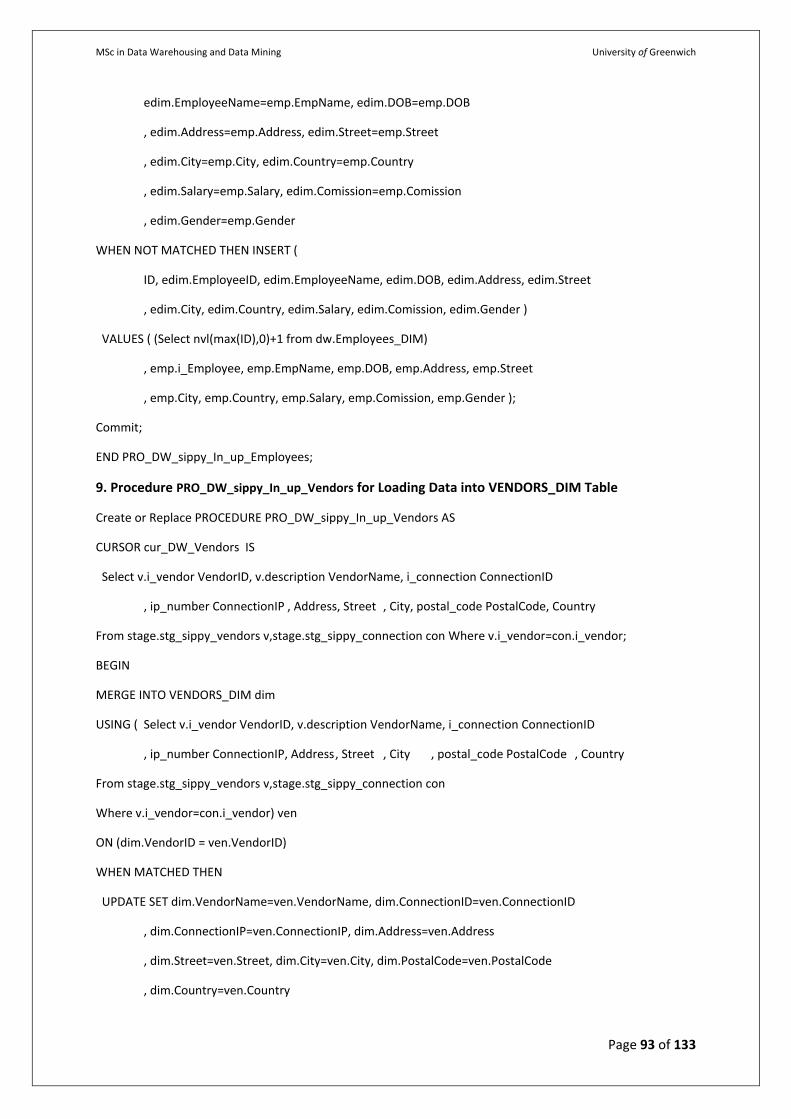
MSc in Data Warehousing and Data Mining University of Greenwich
Page 93 of 133
edim.EmployeeName=emp.EmpName, edim.DOB=emp.DOB
, edim.Address=emp.Address, edim.Street=emp.Street
, edim.City=emp.City, edim.Country=emp.Country
, edim.Salary=emp.Salary, edim.Comission=emp.Comission
, edim.Gender=emp.Gender
WHEN NOT MATCHED THEN INSERT (
ID, edim.EmployeeID, edim.EmployeeName, edim.DOB, edim.Address, edim.Street
, edim.City, edim.Country, edim.Salary, edim.Comission, edim.Gender )
VALUES ( (Select nvl(max(ID),0)+1 from dw.Employees_DIM)
, emp.i_Employee, emp.EmpName, emp.DOB, emp.Address, emp.Street
, emp.City, emp.Country, emp.Salary, emp.Comission, emp.Gender );
Commit;
END PRO_DW_sippy_In_up_Employees;
9. Procedure PRO_DW_sippy_In_up_Vendors for Loading Data into VENDORS_DIM Table
Create or Replace PROCEDURE PRO_DW_sippy_In_up_Vendors AS
CURSOR cur_DW_Vendors IS
Select v.i_vendor VendorID, v.description VendorName, i_connection ConnectionID
, ip_number ConnectionIP , Address, Street , City, postal_code PostalCode, Country
From stage.stg_sippy_vendors v,stage.stg_sippy_connection con Where v.i_vendor=con.i_vendor;
BEGIN
MERGE INTO VENDORS_DIM dim
USING ( Select v.i_vendor VendorID, v.description VendorName, i_connection ConnectionID
, ip_number ConnectionIP, Address , Street , City , postal_code PostalCode , Country
From stage.stg_sippy_vendors v,stage.stg_sippy_connection con
Where v.i_vendor=con.i_vendor) ven
ON (dim.VendorID = ven.VendorID)
WHEN MATCHED THEN
UPDATE SET dim.VendorName=ven.VendorName, dim.ConnectionID=ven.ConnectionID
, dim.ConnectionIP=ven.ConnectionIP, dim.Address=ven.Address
, dim.Street=ven.Street, dim.City=ven.City, dim.PostalCode=ven.PostalCode
, dim.Country=ven.Country
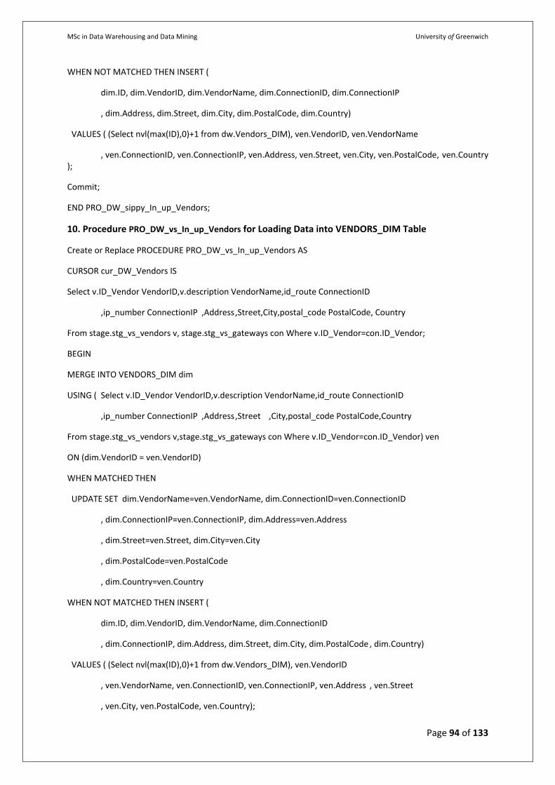
MSc in Data Warehousing and Data Mining University of Greenwich
Page 94 of 133
WHEN NOT MATCHED THEN INSERT (
dim.ID, dim.VendorID, dim.VendorName, dim.ConnectionID, dim.ConnectionIP
, dim.Address, dim.Street, dim.City, dim.PostalCode, dim.Country)
VALUES ( (Select nvl(max(ID),0)+1 from dw.Vendors_DIM), ven.VendorID, ven.VendorName
, ven.ConnectionID, ven.ConnectionIP, ven.Address, ven.Street, ven.City, ven.PostalCode , ven.Country );
Commit;
END PRO_DW_sippy_In_up_Vendors;
10. Procedure PRO_DW_vs_In_up_Vendors for Loading Data into VENDORS_DIM Table
Create or Replace PROCEDURE PRO_DW_vs_In_up_Vendors AS
CURSOR cur_DW_Vendors IS
Select v.ID_Vendor VendorID,v.description VendorName,id_route ConnectionID
,ip_number ConnectionIP ,Address ,Street,City,postal_code PostalCode, Country
From stage.stg_vs_vendors v, stage.stg_vs_gateways con Where v.ID_Vendor=con.ID_Vendor;
BEGIN
MERGE INTO VENDORS_DIM dim
USING ( Select v.ID_Vendor VendorID,v.description VendorName,id_route ConnectionID
,ip_number ConnectionIP ,Address ,Street ,City,postal_code PostalCode,Country
From stage.stg_vs_vendors v,stage.stg_vs_gateways con Where v.ID_Vendor=con.ID_Vendor) ven
ON (dim.VendorID = ven.VendorID)
WHEN MATCHED THEN
UPDATE SET dim.VendorName=ven.VendorName, dim.ConnectionID=ven.ConnectionID
, dim.ConnectionIP=ven.ConnectionIP, dim.Address=ven.Address
, dim.Street=ven.Street, dim.City=ven.City
, dim.PostalCode=ven.PostalCode
, dim.Country=ven.Country
WHEN NOT MATCHED THEN INSERT (
dim.ID, dim.VendorID, dim.VendorName, dim.ConnectionID
, dim.ConnectionIP, dim.Address, dim.Street , dim.City, dim.PostalCode , dim.Country)
VALUES ( (Select nvl(max(ID),0)+1 from dw.Vendors_DIM), ven.VendorID
, ven.VendorName, ven.ConnectionID, ven.ConnectionIP, ven.Address , ven.Street
, ven.City, ven.PostalCode, ven.Country);
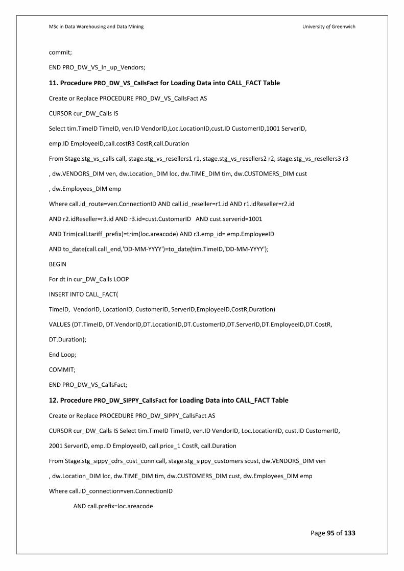
MSc in Data Warehousing and Data Mining University of Greenwich
Page 95 of 133
commit;
END PRO_DW_VS_In_up_Vendors;
11. Procedure PRO_DW_VS_CallsFact for Loading Data into CALL_FACT Table
Create or Replace PROCEDURE PRO_DW_VS_CallsFact AS
CURSOR cur_DW_Calls IS
Select tim.TimeID TimeID, ven.ID VendorID,Loc.LocationID,cust.ID CustomerID,1001 ServerID,
emp.ID EmployeeID,call.costR3 CostR,call.Duration
From Stage.stg_vs_calls call, stage.stg_vs_resellers1 r1, stage.stg_vs_resellers2 r2, stage.stg_vs_resellers3 r3
, dw.VENDORS_DIM ven, dw.Location_DIM loc, dw.TIME_DIM tim, dw.CUSTOMERS_DIM cust
, dw.Employees_DIM emp
Where call.id_route=ven.ConnectionID AND call.id_reseller=r1.id AND r1.idReseller=r2.id
AND r2.idReseller=r3.id AND r3.id=cust.CustomerID AND cust.serverid=1001
AND Trim(call.tariff_prefix)=trim(loc.areacode) AND r3.emp_id= emp.EmployeeID
AND to_date(call.call_end,'DD-MM-YYYY')=to_date(tim.TimeID,'DD-MM-YYYY');
BEGIN
For dt in cur_DW_Calls LOOP
INSERT INTO CALL_FACT(
TimeID, VendorID, LocationID, CustomerID, ServerID,EmployeeID,CostR,Duration)
VALUES (DT.TimeID, DT.VendorID,DT.LocationID,DT.CustomerID,DT.ServerID,DT.EmployeeID,DT.CostR,
DT.Duration);
End Loop;
COMMIT;
END PRO_DW_VS_CallsFact;
12. Procedure PRO_DW_SIPPY_CallsFact for Loading Data into CALL_FACT Table
Create or Replace PROCEDURE PRO_DW_SIPPY_CallsFact AS
CURSOR cur_DW_Calls IS Select tim.TimeID TimeID, ven.ID VendorID, Loc.LocationID, cust.ID CustomerID,
2001 ServerID, emp.ID EmployeeID, call.price_1 CostR, call.Duration
From Stage.stg_sippy_cdrs_cust_conn call, stage.stg_sippy_customers scust, dw.VENDORS_DIM ven
, dw.Location_DIM loc, dw.TIME_DIM tim, dw.CUSTOMERS_DIM cust, dw.Employees_DIM emp
Where call.iD_connection=ven.ConnectionID
AND call.prefix=loc.areacode
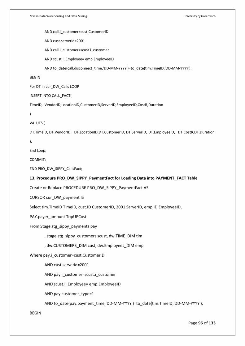
MSc in Data Warehousing and Data Mining University of Greenwich
Page 96 of 133
AND call.i_customer=cust.CustomerID
AND cust.serverid=2001
AND call.i_customer=scust.i_customer
AND scust.i_Employee= emp.EmployeeID
AND to_date(call.disconnect_time,'DD-MM-YYYY')=to_date(tim.TimeID,'DD-MM-YYYY');
BEGIN
For DT in cur_DW_Calls LOOP
INSERT INTO CALL_FACT(
TimeID, VendorID,LocationID,CustomerID,ServerID,EmployeeID,CostR, Duration
)
VALUES (
DT.TimeID, DT.VendorID, DT.LocationID,DT.CustomerID, DT.ServerID, DT.EmployeeID, DT.CostR,DT.Duration
);
End Loop;
COMMIT;
END PRO_DW_SIPPY_CallsFact;
13. Procedure PRO_DW_SIPPY_PaymentFact for Loading Data into PAYMENT_FACT Table
Create or Replace PROCEDURE PRO_DW_SIPPY_PaymentFact AS
CURSOR cur_DW_payment IS
Select tim.TimeID TimeID, cust.ID CustomerID, 2001 ServerID, emp.ID EmployeeID,
PAY.payer_amount TopUPCost
From Stage.stg_sippy_payments pay
, stage.stg_sippy_customers scust, dw.TIME_DIM tim
, dw.CUSTOMERS_DIM cust, dw.Employees_DIM emp
Where pay.i_customer=cust.CustomerID
AND cust.serverid=2001
AND pay.i_customer=scust.i_customer
AND scust.i_Employee= emp.EmployeeID
AND pay.customer_type=1
AND to_date(pay.payment_time,'DD-MM-YYYY')=to_date(tim.TimeID,'DD-MM-YYYY');
BEGIN
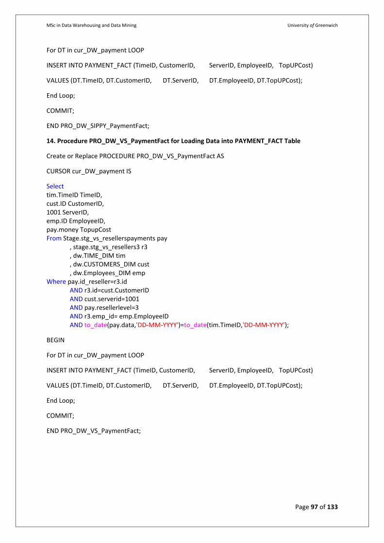
MSc in Data Warehousing and Data Mining University of Greenwich
Page 97 of 133
For DT in cur_DW_payment LOOP
INSERT INTO PAYMENT_FACT (TimeID, CustomerID, ServerID, EmployeeID, TopUPCost)
VALUES (DT.TimeID, DT.CustomerID, DT.ServerID, DT.EmployeeID, DT.TopUPCost);
End Loop;
COMMIT;
END PRO_DW_SIPPY_PaymentFact;
14. Procedure PRO_DW_VS_PaymentFact for Loading Data into PAYMENT_FACT Table
Create or Replace PROCEDURE PRO_DW_VS_PaymentFact AS
CURSOR cur_DW_payment IS
Select tim.TimeID TimeID, cust.ID CustomerID, 1001 ServerID, emp.ID EmployeeID, pay.money TopupCost From Stage.stg_vs_resellerspayments pay , stage.stg_vs_resellers3 r3 , dw.TIME_DIM tim , dw.CUSTOMERS_DIM cust , dw.Employees_DIM emp Where pay.id_reseller=r3.id AND r3.id=cust.CustomerID AND cust.serverid=1001 AND pay.resellerlevel=3 AND r3.emp_id= emp.EmployeeID AND to_date(pay.data,'DD-MM-YYYY')=to_date(tim.TimeID,'DD-MM-YYYY');
BEGIN
For DT in cur_DW_payment LOOP
INSERT INTO PAYMENT_FACT (TimeID, CustomerID, ServerID, EmployeeID, TopUPCost)
VALUES (DT.TimeID, DT.CustomerID, DT.ServerID, DT.EmployeeID, DT.TopUPCost);
End Loop;
COMMIT;
END PRO_DW_VS_PaymentFact;
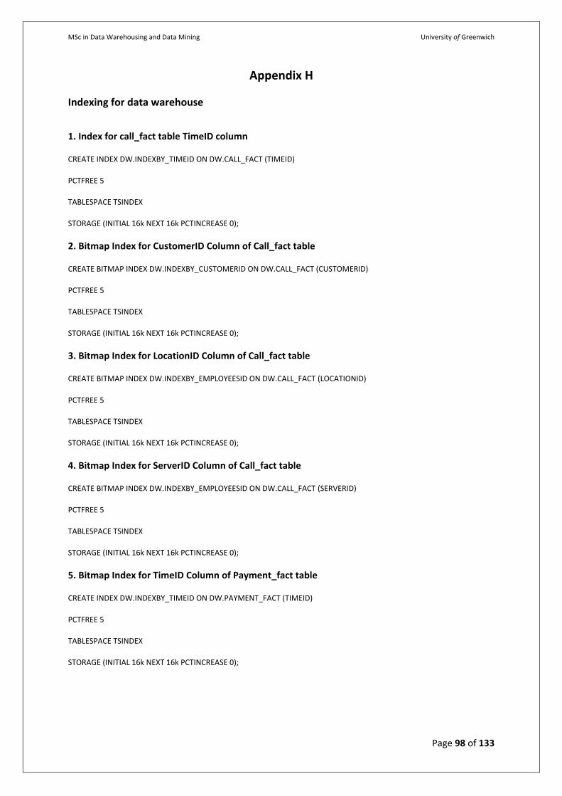
MSc in Data Warehousing and Data Mining University of Greenwich
Page 98 of 133
Appendix H
Indexing for data warehouse
1. Index for call_fact table TimeID column
CREATE INDEX DW.INDEXBY_TIMEID ON DW.CALL_FACT (TIMEID)
PCTFREE 5
TABLESPACE TSINDEX
STORAGE (INITIAL 16k NEXT 16k PCTINCREASE 0);
2. Bitmap Index for CustomerID Column of Call_fact table
CREATE BITMAP INDEX DW.INDEXBY_CUSTOMERID ON DW.CALL_FACT (CUSTOMERID)
PCTFREE 5
TABLESPACE TSINDEX
STORAGE (INITIAL 16k NEXT 16k PCTINCREASE 0);
3. Bitmap Index for LocationID Column of Call_fact table
CREATE BITMAP INDEX DW.INDEXBY_EMPLOYEESID ON DW.CALL_FACT (LOCATIONID)
PCTFREE 5
TABLESPACE TSINDEX
STORAGE (INITIAL 16k NEXT 16k PCTINCREASE 0);
4. Bitmap Index for ServerID Column of Call_fact table
CREATE BITMAP INDEX DW.INDEXBY_EMPLOYEESID ON DW.CALL_FACT (SERVERID)
PCTFREE 5
TABLESPACE TSINDEX
STORAGE (INITIAL 16k NEXT 16k PCTINCREASE 0);
5. Bitmap Index for TimeID Column of Payment_fact table
CREATE INDEX DW.INDEXBY_TIMEID ON DW.PAYMENT_FACT (TIMEID)
PCTFREE 5
TABLESPACE TSINDEX
STORAGE (INITIAL 16k NEXT 16k PCTINCREASE 0);
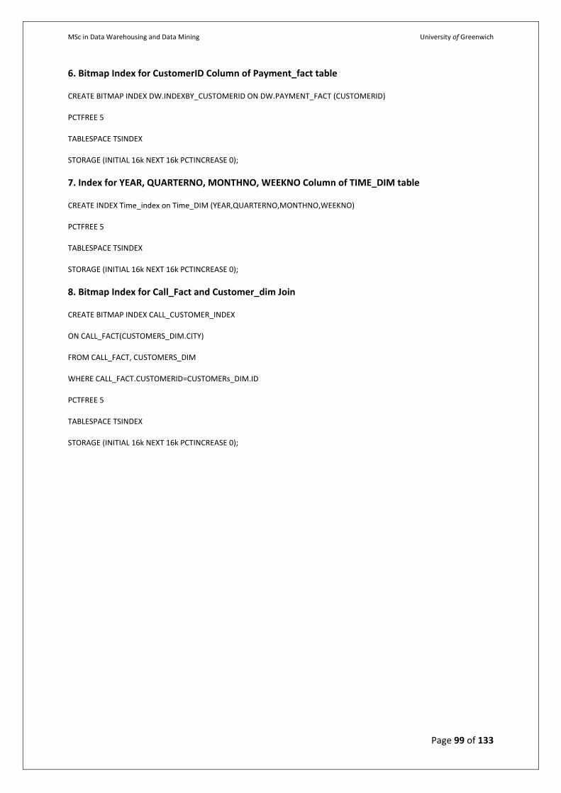
MSc in Data Warehousing and Data Mining University of Greenwich
Page 99 of 133
6. Bitmap Index for CustomerID Column of Payment_fact table
CREATE BITMAP INDEX DW.INDEXBY_CUSTOMERID ON DW.PAYMENT_FACT (CUSTOMERID)
PCTFREE 5
TABLESPACE TSINDEX
STORAGE (INITIAL 16k NEXT 16k PCTINCREASE 0);
7. Index for YEAR, QUARTERNO, MONTHNO, WEEKNO Column of TIME_DIM table
CREATE INDEX Time_index on Time_DIM (YEAR,QUARTERNO,MONTHNO,WEEKNO)
PCTFREE 5
TABLESPACE TSINDEX
STORAGE (INITIAL 16k NEXT 16k PCTINCREASE 0);
8. Bitmap Index for Call_Fact and Customer_dim Join
CREATE BITMAP INDEX CALL_CUSTOMER_INDEX
ON CALL_FACT(CUSTOMERS_DIM.CITY)
FROM CALL_FACT, CUSTOMERS_DIM
WHERE CALL_FACT.CUSTOMERID=CUSTOMERs_DIM.ID
PCTFREE 5
TABLESPACE TSINDEX
STORAGE (INITIAL 16k NEXT 16k PCTINCREASE 0);
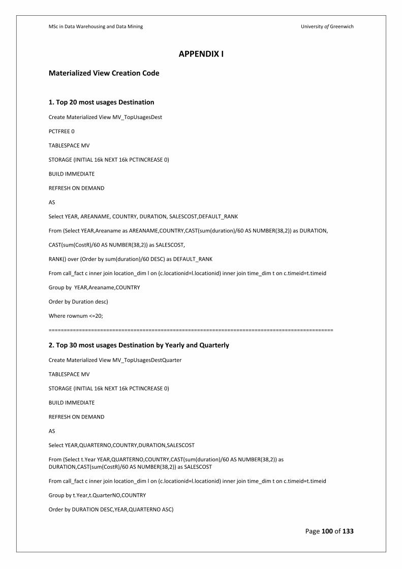
MSc in Data Warehousing and Data Mining University of Greenwich
Page 100 of 133
APPENDIX I
Materialized View Creation Code
1. Top 20 most usages Destination
Create Materialized View MV_TopUsagesDest
PCTFREE 0
TABLESPACE MV
STORAGE (INITIAL 16k NEXT 16k PCTINCREASE 0)
BUILD IMMEDIATE
REFRESH ON DEMAND
AS
Select YEAR, AREANAME, COUNTRY, DURATION, SALESCOST,DEFAULT_RANK
From (Select YEAR,Areaname as AREANAME,COUNTRY,CAST(sum(duration)/60 AS NUMBER(38,2)) as DURATION,
CAST(sum(CostR)/60 AS NUMBER(38,2)) as SALESCOST,
RANK() over (Order by sum(duration)/60 DESC) as DEFAULT_RANK
From call_fact c inner join location_dim l on (c.locationid=l.locationid) inner join time_dim t on c.timeid=t.timeid
Group by YEAR,Areaname,COUNTRY
Order by Duration desc)
Where rownum <=20;
==============================================================================================
2. Top 30 most usages Destination by Yearly and Quarterly
Create Materialized View MV_TopUsagesDestQuarter
TABLESPACE MV
STORAGE (INITIAL 16k NEXT 16k PCTINCREASE 0)
BUILD IMMEDIATE
REFRESH ON DEMAND
AS
Select YEAR,QUARTERNO,COUNTRY,DURATION,SALESCOST
From (Select t.Year YEAR,QUARTERNO,COUNTRY,CAST(sum(duration)/60 AS NUMBER(38,2)) as DURATION,CAST(sum(CostR)/60 AS NUMBER(38,2)) as SALESCOST
From call_fact c inner join location_dim l on (c.locationid=l.locationid) inner join time_dim t on c.timeid=t.timeid
Group by t.Year,t.QuarterNO,COUNTRY
Order by DURATION DESC,YEAR,QUARTERNO ASC)
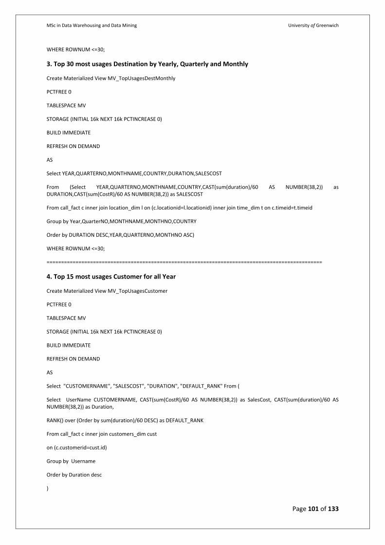
MSc in Data Warehousing and Data Mining University of Greenwich
Page 101 of 133
WHERE ROWNUM <=30;
3. Top 30 most usages Destination by Yearly, Quarterly and Monthly
Create Materialized View MV_TopUsagesDestMonthly
PCTFREE 0
TABLESPACE MV
STORAGE (INITIAL 16k NEXT 16k PCTINCREASE 0)
BUILD IMMEDIATE
REFRESH ON DEMAND
AS
Select YEAR,QUARTERNO,MONTHNAME,COUNTRY,DURATION,SALESCOST
From (Select YEAR,QUARTERNO,MONTHNAME,COUNTRY,CAST(sum(duration)/60 AS NUMBER(38,2)) as DURATION,CAST(sum(CostR)/60 AS NUMBER(38,2)) as SALESCOST
From call_fact c inner join location_dim l on (c.locationid=l.locationid) inner join time_dim t on c.timeid=t.timeid
Group by Year,QuarterNO,MONTHNAME,MONTHNO,COUNTRY
Order by DURATION DESC,YEAR,QUARTERNO,MONTHNO ASC)
WHERE ROWNUM <=30;
===============================================================================================
4. Top 15 most usages Customer for all Year
Create Materialized View MV_TopUsagesCustomer
PCTFREE 0
TABLESPACE MV
STORAGE (INITIAL 16k NEXT 16k PCTINCREASE 0)
BUILD IMMEDIATE
REFRESH ON DEMAND
AS
Select "CUSTOMERNAME", "SALESCOST", "DURATION", "DEFAULT_RANK" From (
Select UserName CUSTOMERNAME, CAST(sum(CostR)/60 AS NUMBER(38,2)) as SalesCost, CAST(sum(duration)/60 AS NUMBER(38,2)) as Duration,
RANK() over (Order by sum(duration)/60 DESC) as DEFAULT_RANK
From call_fact c inner join customers_dim cust
on (c.customerid=cust.id)
Group by Username
Order by Duration desc
)
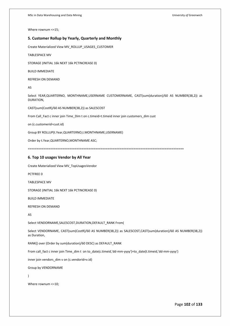
MSc in Data Warehousing and Data Mining University of Greenwich
Page 102 of 133
Where rownum <=15;
5. Customer Rollup by Yearly, Quarterly and Monthly
Create Materialized View MV_ROLLUP_USAGES_CUSTOMER
TABLESPACE MV
STORAGE (INITIAL 16k NEXT 16k PCTINCREASE 0)
BUILD IMMEDIATE
REFRESH ON DEMAND
AS
Select YEAR,QUARTERNO, MONTHNAME,USERNAME CUSTOMERNAME, CAST(sum(duration)/60 AS NUMBER(38,2)) as DURATION,
CAST(sum(CostR)/60 AS NUMBER(38,2)) as SALESCOST
From Call_Fact c inner join Time_Dim t on c.timeid=t.timeid inner join customers_dim cust
on (c.customerid=cust.id)
Group BY ROLLUP(t.Year,QUARTERNO,t.MONTHNAME,USERNAME)
Order by t.Year,QUARTERNO,MONTHNAME ASC;
==========================================================================================
6. Top 10 usages Vendor by All Year
Create Materialized View MV_TopUsagesVendor
PCTFREE 0
TABLESPACE MV
STORAGE (INITIAL 16k NEXT 16k PCTINCREASE 0)
BUILD IMMEDIATE
REFRESH ON DEMAND
AS
Select VENDORNAME,SALESCOST,DURATION,DEFAULT_RANK From(
Select VENDORNAME, CAST(sum(CostR)/60 AS NUMBER(38,2)) as SALESCOST,CAST(sum(duration)/60 AS NUMBER(38,2)) as Duration,
RANK() over (Order by sum(duration)/60 DESC) as DEFAULT_RANK
From call_fact c inner join Time_dim t on to_date(c.timeid,'dd-mm-yyyy')=to_date(t.timeid,'dd-mm-yyyy')
inner join vendors_dim v on (c.vendorid=v.id)
Group by VENDORNAME
)
Where rownum <=10;
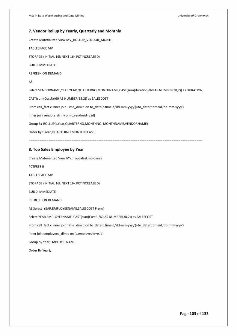
MSc in Data Warehousing and Data Mining University of Greenwich
Page 103 of 133
7. Vendor Rollup by Yearly, Quarterly and Monthly
Create Materialized View MV_ROLLUP_VENDOR_MONTH
TABLESPACE MV
STORAGE (INITIAL 16k NEXT 16k PCTINCREASE 0)
BUILD IMMEDIATE
REFRESH ON DEMAND
AS
Select VENDORNAME,YEAR YEAR,QUARTERNO,MONTHNAME,CAST(sum(duration)/60 AS NUMBER(38,2)) as DURATION,
CAST(sum(CostR)/60 AS NUMBER(38,2)) as SALESCOST
From call_fact c inner join Time_dim t on to_date(c.timeid,'dd-mm-yyyy')=to_date(t.timeid,'dd-mm-yyyy')
Inner join vendors_dim v on (c.vendorid=v.id)
Group BY ROLLUP(t.Year,QUARTERNO,MONTHNO, MONTHNAME,VENDORNAME)
Order by t.Year,QUARTERNO,MONTHNO ASC;
=================================================================================================
8. Top Sales Employee by Year
Create Materialized View MV_TopSalesEmployees
PCTFREE 0
TABLESPACE MV
STORAGE (INITIAL 16k NEXT 16k PCTINCREASE 0)
BUILD IMMEDIATE
REFRESH ON DEMAND
AS Select YEAR,EMPLOYEENAME,SALESCOST From(
Select YEAR,EMPLOYEENAME, CAST(sum(CostR)/60 AS NUMBER(38,2)) as SALESCOST
From call_fact c inner join Time_dim t on to_date(c.timeid,'dd-mm-yyyy')=to_date(t.timeid,'dd-mm-yyyy')
inner join employees_dim e on (c.employeeid=e.id)
Group by Year,EMPLOYEENAME
Order By Year);
MSc in Data Warehousing and Data Mining University of Greenwich
Page 104 of 133
9. Employee Rollup by Yearly, Quarterly and Monthly
Create Materialized View MV_ROLLUP_EMPLOYEE_MONTH
TABLESPACE MV
STORAGE (INITIAL 16k NEXT 16k PCTINCREASE 0)
BUILD IMMEDIATE
REFRESH ON DEMAND
AS
Select EMPLOYEENAME, YEAR, QUARTERNO, MONTHNAME, CAST(sum(duration)/60 AS NUMBER(38,2)) as DURATION,
CAST(sum(CostR)/60 AS NUMBER(38,2)) as SALESCOST
From call_fact c Inner Join Time_Dim t on TO_Date(c.timeid,'dd-mm-yyyy')=TO_Date(t.timeid,'dd-mm-yyyy')
Inner Join Employees_Dim e on (c.employeeid=e.id)
Group BY ROLLUP(Year,QUARTERNO,MONTHNO, MONTHNAME, EMPLOYEENAME)
Order by t.Year,QUARTERNO,MONTHNO, MONTHNAME ASC;
=================================================================================================
10. Top Usages by Yearly, Quarterly and Monthly
Create Materialized View MV_TopUsagesMonthly
TABLESPACE MV
STORAGE (INITIAL 16k NEXT 16k PCTINCREASE 0)
BUILD IMMEDIATE
REFRESH ON DEMAND
AS
Select YEAR YEAR,QuarterDesc QUARTERDESC, MonthName MONTHNAME, CAST(sum(duration)/60 AS NUMBER(38,2)) as DURATION,
CAST(sum(CostR)/60 AS NUMBER(38,2)) as SALESCOST
From call_fact c inner join time_dim t on c.timeid=t.timeid
Group by t.Year,t.QuarterDesc,MonthName
Order by Duration desc;
==============================================================================================
11. Usages Rollup by Yearly, Quarterly and Monthly
Create Materialized View MV_ROLLUP_USAGES_MONTH
TABLESPACE MV
STORAGE (INITIAL 16k NEXT 16k PCTINCREASE 0)
BUILD IMMEDIATE
MSc in Data Warehousing and Data Mining University of Greenwich
Page 105 of 133
REFRESH ON DEMAND
AS
Select YEAR YEAR,QUARTERNO,MONTHNAME,CAST(sum(duration)/60 AS NUMBER(38,2)) as DURATION,
CAST(sum(CostR)/60 AS NUMBER(38,2)) as SALESCOST
From call_fact c inner join time_dim t on c.timeid=t.timeid
Group BY ROLLUP(t.Year,QUARTERNO,t.MONTHNAME)
Order by t.Year,QUARTERNO ASC;
=================================================================================================
12. Usages Employee and Customer CUBE by Yearly, Quarterly and Monthly
Create Materialized View MV_CUBE_EMPL_CUST_YEAR
TABLESPACE MV
STORAGE (INITIAL 16k NEXT 16k PCTINCREASE 0)
BUILD IMMEDIATE
REFRESH ON DEMAND
AS
Select EMPLOYEENAME,USERNAME CUSTOMERNAME, YEAR, CAST(sum(duration)/60 AS NUMBER(38,2)) as DURATION,
CAST(sum(CostR)/60 AS NUMBER(38,2)) as SALESCOST
From Call_Fact c Inner Join Time_Dim t on TO_Date(c.timeid,'dd-mm-yyyy')=TO_Date(t.timeid,'dd-mm-yyyy')
Inner Join Employees_Dim e on (c.employeeid=e.id) Inner Join CUSTOMERS_Dim CUST on (c.CUSTOMERID=CUST.id)
Group BY CUBE(Year,EMPLOYEENAME,USERNAME)
Order by Year,EMPLOYEENAME,USERNAME ASC;
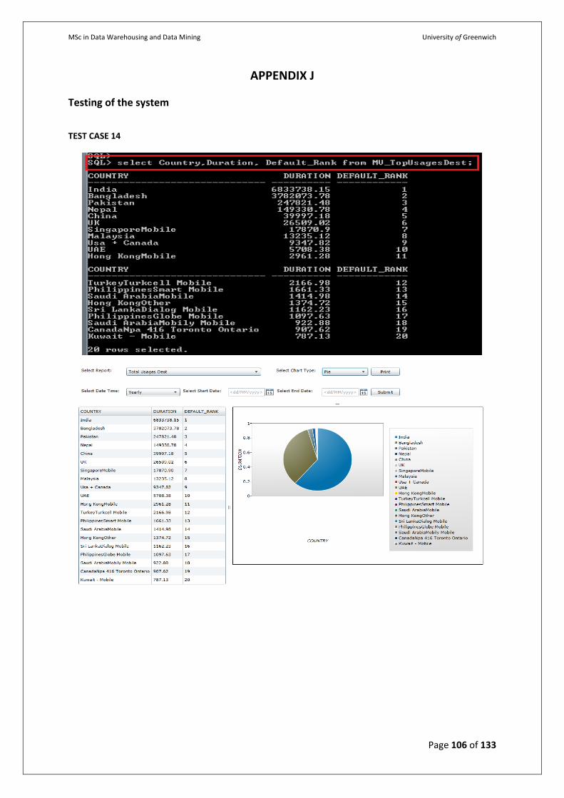
MSc in Data Warehousing and Data Mining University of Greenwich
Page 106 of 133
APPENDIX J
Testing of the system
TEST CASE 14
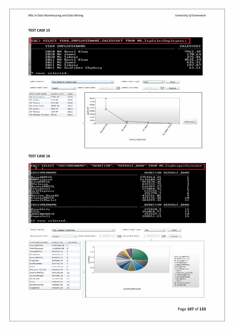
MSc in Data Warehousing and Data Mining University of Greenwich
Page 107 of 133
TEST CASE 15
TEST CASE 16
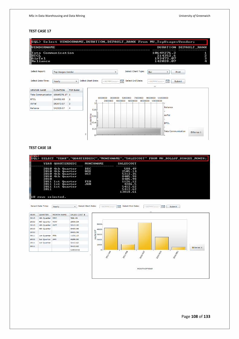
MSc in Data Warehousing and Data Mining University of Greenwich
Page 108 of 133
TEST CASE 17
TEST CASE 18
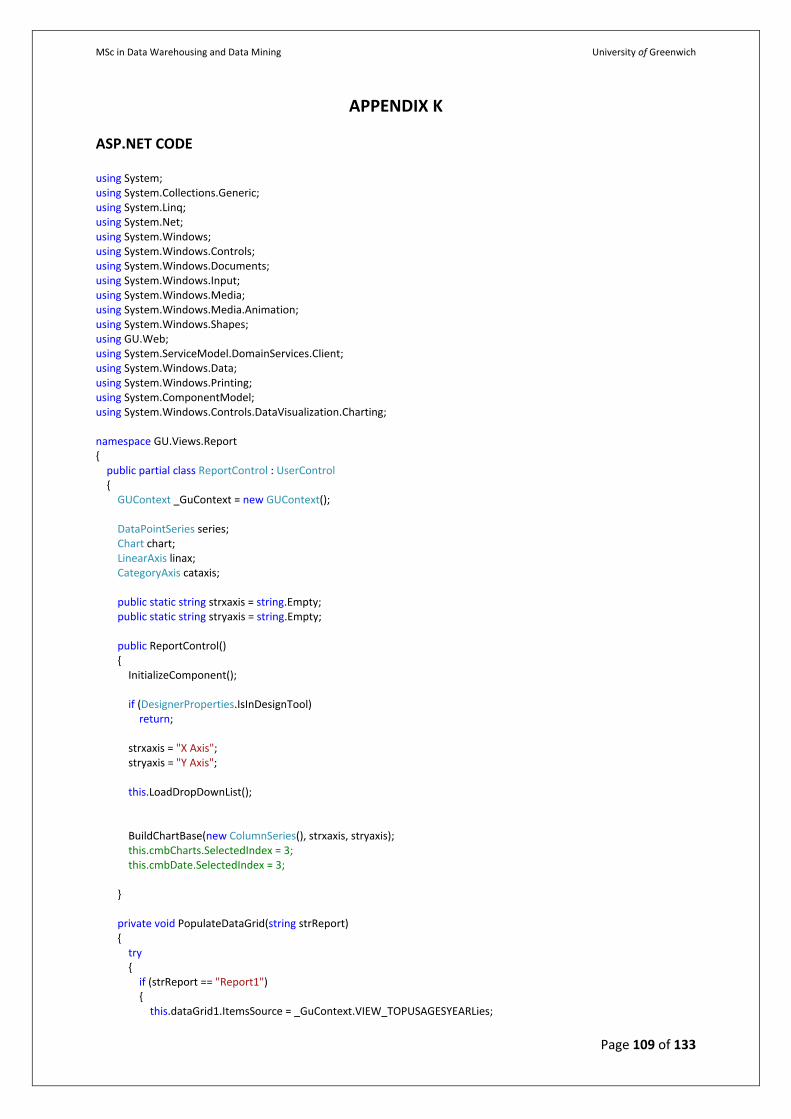
MSc in Data Warehousing and Data Mining University of Greenwich
Page 109 of 133
APPENDIX K
ASP.NET CODE using System; using System.Collections.Generic; using System.Linq; using System.Net; using System.Windows; using System.Windows.Controls; using System.Windows.Documents; using System.Windows.Input; using System.Windows.Media; using System.Windows.Media.Animation; using System.Windows.Shapes; using GU.Web; using System.ServiceModel.DomainServices.Client; using System.Windows.Data; using System.Windows.Printing; using System.ComponentModel; using System.Windows.Controls.DataVisualization.Charting; namespace GU.Views.Report { public partial class ReportControl : UserControl { GUContext _GuContext = new GUContext(); DataPointSeries series; Chart chart; LinearAxis linax; CategoryAxis cataxis; public static string strxaxis = string.Empty; public static string stryaxis = string.Empty; public ReportControl() { InitializeComponent(); if (DesignerProperties.IsInDesignTool) return; strxaxis = "X Axis"; stryaxis = "Y Axis"; this.LoadDropDownList(); BuildChartBase(new ColumnSeries(), strxaxis, stryaxis); this.cmbCharts.SelectedIndex = 3; this.cmbDate.SelectedIndex = 3; } private void PopulateDataGrid(string strReport) { try { if (strReport == "Report1") { this.dataGrid1.ItemsSource = _GuContext.VIEW_TOPUSAGESYEARLies;
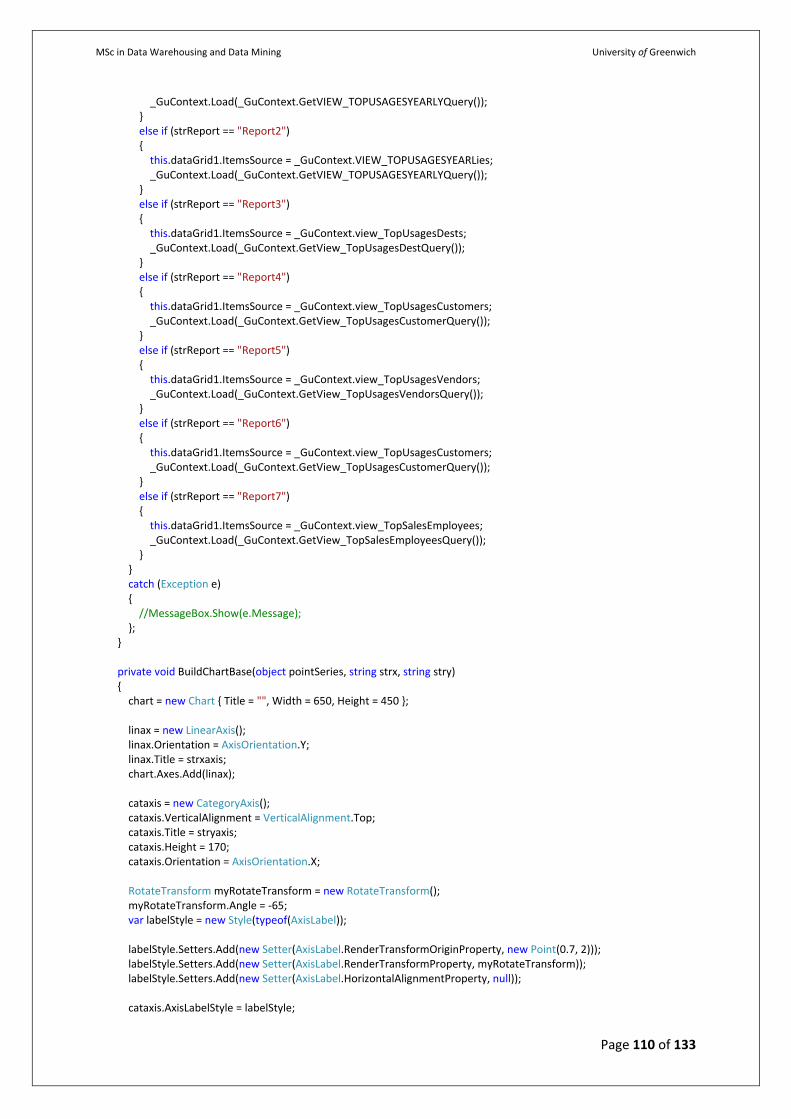
MSc in Data Warehousing and Data Mining University of Greenwich
Page 110 of 133
_GuContext.Load(_GuContext.GetVIEW_TOPUSAGESYEARLYQuery()); } else if (strReport == "Report2") { this.dataGrid1.ItemsSource = _GuContext.VIEW_TOPUSAGESYEARLies; _GuContext.Load(_GuContext.GetVIEW_TOPUSAGESYEARLYQuery()); } else if (strReport == "Report3") { this.dataGrid1.ItemsSource = _GuContext.view_TopUsagesDests; _GuContext.Load(_GuContext.GetView_TopUsagesDestQuery()); } else if (strReport == "Report4") { this.dataGrid1.ItemsSource = _GuContext.view_TopUsagesCustomers; _GuContext.Load(_GuContext.GetView_TopUsagesCustomerQuery()); } else if (strReport == "Report5") { this.dataGrid1.ItemsSource = _GuContext.view_TopUsagesVendors; _GuContext.Load(_GuContext.GetView_TopUsagesVendorsQuery()); } else if (strReport == "Report6") { this.dataGrid1.ItemsSource = _GuContext.view_TopUsagesCustomers; _GuContext.Load(_GuContext.GetView_TopUsagesCustomerQuery()); } else if (strReport == "Report7") { this.dataGrid1.ItemsSource = _GuContext.view_TopSalesEmployees; _GuContext.Load(_GuContext.GetView_TopSalesEmployeesQuery()); } } catch (Exception e) { //MessageBox.Show(e.Message); }; } private void BuildChartBase(object pointSeries, string strx, string stry) { chart = new Chart { Title = "", Width = 650, Height = 450 }; linax = new LinearAxis(); linax.Orientation = AxisOrientation.Y; linax.Title = strxaxis; chart.Axes.Add(linax); cataxis = new CategoryAxis(); cataxis.VerticalAlignment = VerticalAlignment.Top; cataxis.Title = stryaxis; cataxis.Height = 170; cataxis.Orientation = AxisOrientation.X; RotateTransform myRotateTransform = new RotateTransform(); myRotateTransform.Angle = -65; var labelStyle = new Style(typeof(AxisLabel)); labelStyle.Setters.Add(new Setter(AxisLabel.RenderTransformOriginProperty, new Point(0.7, 2))); labelStyle.Setters.Add(new Setter(AxisLabel.RenderTransformProperty, myRotateTransform)); labelStyle.Setters.Add(new Setter(AxisLabel.HorizontalAlignmentProperty, null)); cataxis.AxisLabelStyle = labelStyle;
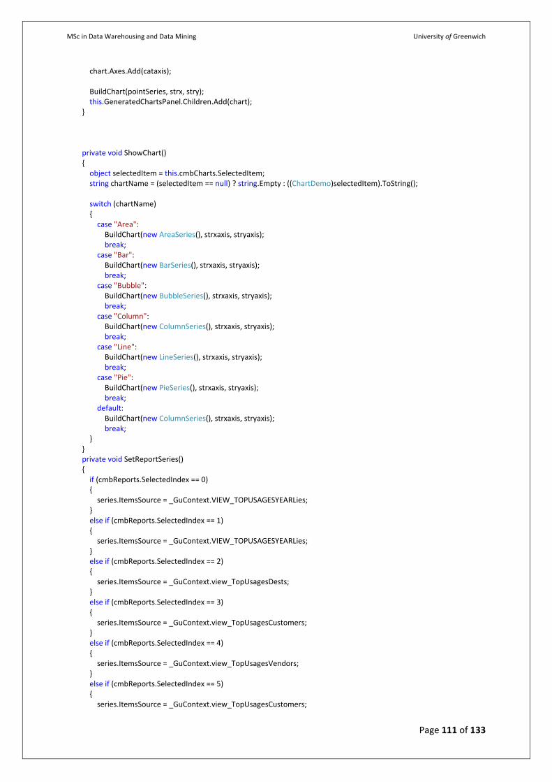
MSc in Data Warehousing and Data Mining University of Greenwich
Page 111 of 133
chart.Axes.Add(cataxis); BuildChart(pointSeries, strx, stry); this.GeneratedChartsPanel.Children.Add(chart); } private void ShowChart() { object selectedItem = this.cmbCharts.SelectedItem; string chartName = (selectedItem == null) ? string.Empty : ((ChartDemo)selectedItem).ToString(); switch (chartName) { case "Area": BuildChart(new AreaSeries(), strxaxis, stryaxis); break; case "Bar": BuildChart(new BarSeries(), strxaxis, stryaxis); break; case "Bubble": BuildChart(new BubbleSeries(), strxaxis, stryaxis); break; case "Column": BuildChart(new ColumnSeries(), strxaxis, stryaxis); break; case "Line": BuildChart(new LineSeries(), strxaxis, stryaxis); break; case "Pie": BuildChart(new PieSeries(), strxaxis, stryaxis); break; default: BuildChart(new ColumnSeries(), strxaxis, stryaxis); break; } } private void SetReportSeries() { if (cmbReports.SelectedIndex == 0) { series.ItemsSource = _GuContext.VIEW_TOPUSAGESYEARLies; } else if (cmbReports.SelectedIndex == 1) { series.ItemsSource = _GuContext.VIEW_TOPUSAGESYEARLies; } else if (cmbReports.SelectedIndex == 2) { series.ItemsSource = _GuContext.view_TopUsagesDests; } else if (cmbReports.SelectedIndex == 3) { series.ItemsSource = _GuContext.view_TopUsagesCustomers; } else if (cmbReports.SelectedIndex == 4) { series.ItemsSource = _GuContext.view_TopUsagesVendors; } else if (cmbReports.SelectedIndex == 5) { series.ItemsSource = _GuContext.view_TopUsagesCustomers;
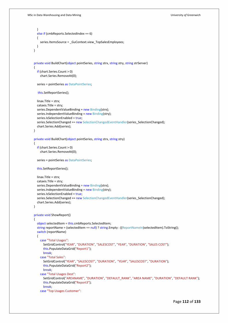
MSc in Data Warehousing and Data Mining University of Greenwich
Page 112 of 133
} else if (cmbReports.SelectedIndex == 6) { series.ItemsSource = _GuContext.view_TopSalesEmployees; } } private void BuildChart(object pointSeries, string strx, string stry, string strServer) { if (chart.Series.Count > 0) chart.Series.RemoveAt(0); series = pointSeries as DataPointSeries; this.SetReportSeries(); linax.Title = strx; cataxis.Title = stry; series.DependentValueBinding = new Binding(strx); series.IndependentValueBinding = new Binding(stry); series.IsSelectionEnabled = true; series.SelectionChanged += new SelectionChangedEventHandler(series_SelectionChanged); chart.Series.Add(series); } private void BuildChart(object pointSeries, string strx, string stry) { if (chart.Series.Count > 0) chart.Series.RemoveAt(0); series = pointSeries as DataPointSeries; this.SetReportSeries(); linax.Title = strx; cataxis.Title = stry; series.DependentValueBinding = new Binding(strx); series.IndependentValueBinding = new Binding(stry); series.IsSelectionEnabled = true; series.SelectionChanged += new SelectionChangedEventHandler(series_SelectionChanged); chart.Series.Add(series); } private void ShowReport() { object selectedItem = this.cmbReports.SelectedItem; string reportName = (selectedItem == null) ? string.Empty : ((ReportNameIn)selectedItem).ToString(); switch (reportName) { case "Total Usages": SetGridControl("YEAR", "DURATION", "SALESCOST", "YEAR", "DURATION", "SALES COST"); this.PopulateDataGrid("Report1"); break; case "Total Sales": SetGridControl("YEAR", "SALESCOST", "DURATION", "YEAR", "SALESCOST", "DURATION"); this.PopulateDataGrid("Report2"); break; case "Total Usages Dest": SetGridControl("AREANAME", "DURATION", "DEFAULT_RANK", "AREA NAME", "DURATION", "DEFAULT RANK"); this.PopulateDataGrid("Report3"); break; case "Top Usages Customer":
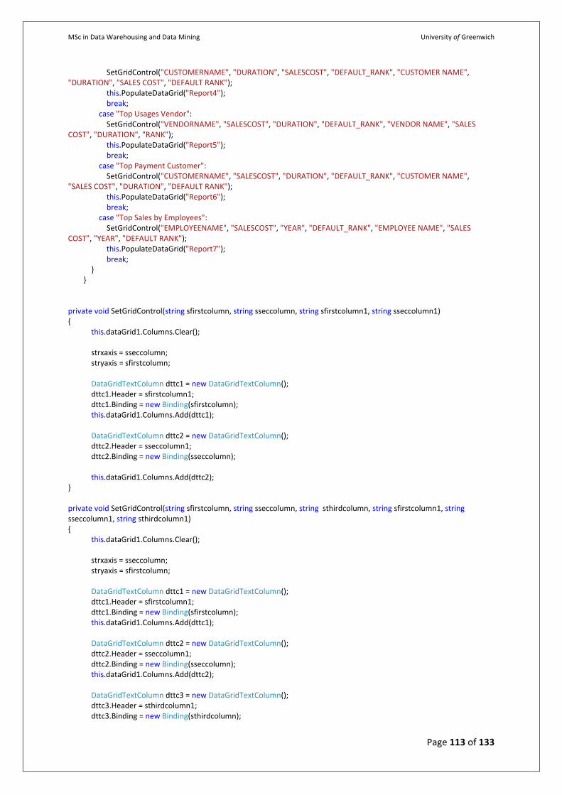
MSc in Data Warehousing and Data Mining University of Greenwich
Page 113 of 133
SetGridControl("CUSTOMERNAME", "DURATION", "SALESCOST", "DEFAULT_RANK", "CUSTOMER NAME", "DURATION", "SALES COST", "DEFAULT RANK"); this.PopulateDataGrid("Report4"); break; case "Top Usages Vendor": SetGridControl("VENDORNAME", "SALESCOST", "DURATION", "DEFAULT_RANK", "VENDOR NAME", "SALES COST", "DURATION", "RANK"); this.PopulateDataGrid("Report5"); break; case "Top Payment Customer": SetGridControl("CUSTOMERNAME", "SALESCOST", "DURATION", "DEFAULT_RANK", "CUSTOMER NAME", "SALES COST", "DURATION", "DEFAULT RANK"); this.PopulateDataGrid("Report6"); break; case "Top Sales by Employees": SetGridControl("EMPLOYEENAME", "SALESCOST", "YEAR", "DEFAULT_RANK", "EMPLOYEE NAME", "SALES COST", "YEAR", "DEFAULT RANK"); this.PopulateDataGrid("Report7"); break; } } private void SetGridControl(string sfirstcolumn, string sseccolumn, string sfirstcolumn1, string sseccolumn1) { this.dataGrid1.Columns.Clear(); strxaxis = sseccolumn; stryaxis = sfirstcolumn; DataGridTextColumn dttc1 = new DataGridTextColumn(); dttc1.Header = sfirstcolumn1; dttc1.Binding = new Binding(sfirstcolumn); this.dataGrid1.Columns.Add(dttc1); DataGridTextColumn dttc2 = new DataGridTextColumn(); dttc2.Header = sseccolumn1; dttc2.Binding = new Binding(sseccolumn); this.dataGrid1.Columns.Add(dttc2); } private void SetGridControl(string sfirstcolumn, string sseccolumn, string sthirdcolumn, string sfirstcolumn1, string sseccolumn1, string sthirdcolumn1) { this.dataGrid1.Columns.Clear(); strxaxis = sseccolumn; stryaxis = sfirstcolumn; DataGridTextColumn dttc1 = new DataGridTextColumn(); dttc1.Header = sfirstcolumn1; dttc1.Binding = new Binding(sfirstcolumn); this.dataGrid1.Columns.Add(dttc1); DataGridTextColumn dttc2 = new DataGridTextColumn(); dttc2.Header = sseccolumn1; dttc2.Binding = new Binding(sseccolumn); this.dataGrid1.Columns.Add(dttc2); DataGridTextColumn dttc3 = new DataGridTextColumn(); dttc3.Header = sthirdcolumn1; dttc3.Binding = new Binding(sthirdcolumn);
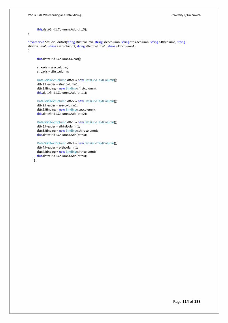
MSc in Data Warehousing and Data Mining University of Greenwich
Page 114 of 133
this.dataGrid1.Columns.Add(dttc3); } private void SetGridControl(string sfirstcolumn, string sseccolumn, string sthirdcolumn, string s4thcolumn, string sfirstcolumn1, string sseccolumn1, string sthirdcolumn1, string s4thcolumn1) { this.dataGrid1.Columns.Clear(); strxaxis = sseccolumn; stryaxis = sfirstcolumn; DataGridTextColumn dttc1 = new DataGridTextColumn(); dttc1.Header = sfirstcolumn1; dttc1.Binding = new Binding(sfirstcolumn); this.dataGrid1.Columns.Add(dttc1); DataGridTextColumn dttc2 = new DataGridTextColumn(); dttc2.Header = sseccolumn1; dttc2.Binding = new Binding(sseccolumn); this.dataGrid1.Columns.Add(dttc2); DataGridTextColumn dttc3 = new DataGridTextColumn(); dttc3.Header = sthirdcolumn1; dttc3.Binding = new Binding(sthirdcolumn); this.dataGrid1.Columns.Add(dttc3); DataGridTextColumn dttc4 = new DataGridTextColumn(); dttc4.Header = s4thcolumn1; dttc4.Binding = new Binding(s4thcolumn); this.dataGrid1.Columns.Add(dttc4); }
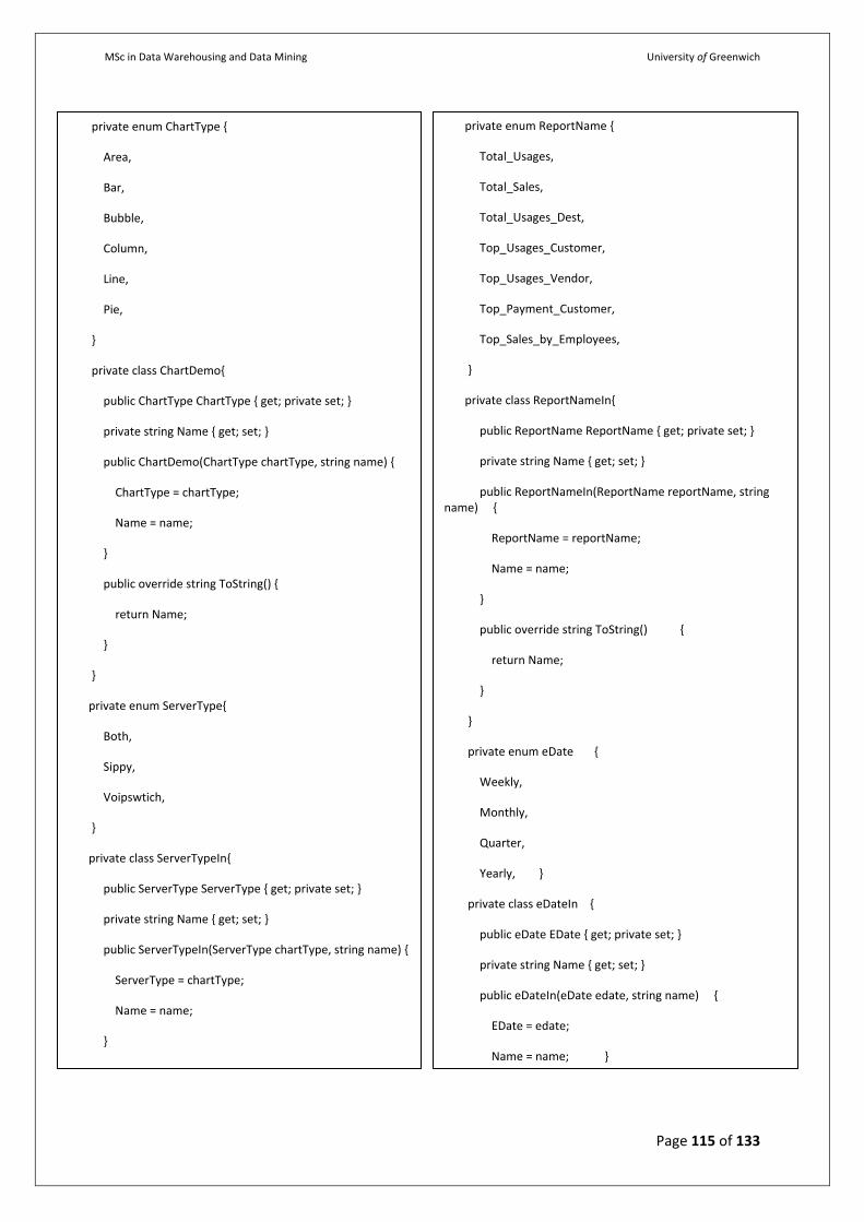
MSc in Data Warehousing and Data Mining University of Greenwich
Page 115 of 133
private enum ChartType {
Area,
Bar,
Bubble,
Column,
Line,
Pie,
}
private class ChartDemo{
public ChartType ChartType { get; private set; }
private string Name { get; set; }
public ChartDemo(ChartType chartType, string name) {
ChartType = chartType;
Name = name;
}
public override string ToString() {
return Name;
}
}
private enum ServerType{
Both,
Sippy,
Voipswtich,
}
private class ServerTypeIn{
public ServerType ServerType { get; private set; }
private string Name { get; set; }
public ServerTypeIn(ServerType chartType, string name) {
ServerType = chartType;
Name = name;
}
private enum ReportName {
Total_Usages,
Total_Sales,
Total_Usages_Dest,
Top_Usages_Customer,
Top_Usages_Vendor,
Top_Payment_Customer,
Top_Sales_by_Employees,
}
private class ReportNameIn{
public ReportName ReportName { get; private set; }
private string Name { get; set; }
public ReportNameIn(ReportName reportName, string name) {
ReportName = reportName;
Name = name;
}
public override string ToString() {
return Name;
}
}
private enum eDate {
Weekly,
Monthly,
Quarter,
Yearly, }
private class eDateIn {
public eDate EDate { get; private set; }
private string Name { get; set; }
public eDateIn(eDate edate, string name) {
EDate = edate;
Name = name; }
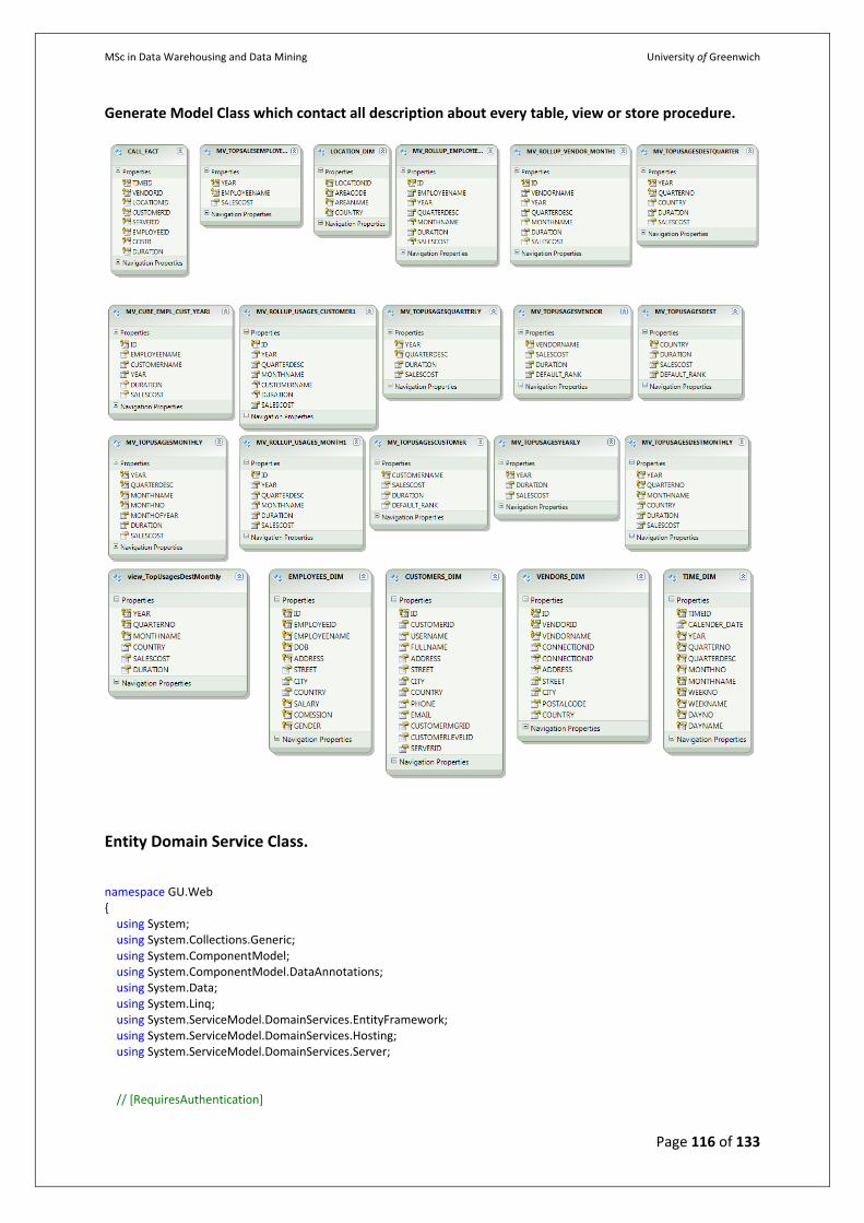
MSc in Data Warehousing and Data Mining University of Greenwich
Page 116 of 133
Generate Model Class which contact all description about every table, view or store procedure.
Entity Domain Service Class. namespace GU.Web { using System; using System.Collections.Generic; using System.ComponentModel; using System.ComponentModel.DataAnnotations; using System.Data; using System.Linq; using System.ServiceModel.DomainServices.EntityFramework; using System.ServiceModel.DomainServices.Hosting; using System.ServiceModel.DomainServices.Server; // [RequiresAuthentication]
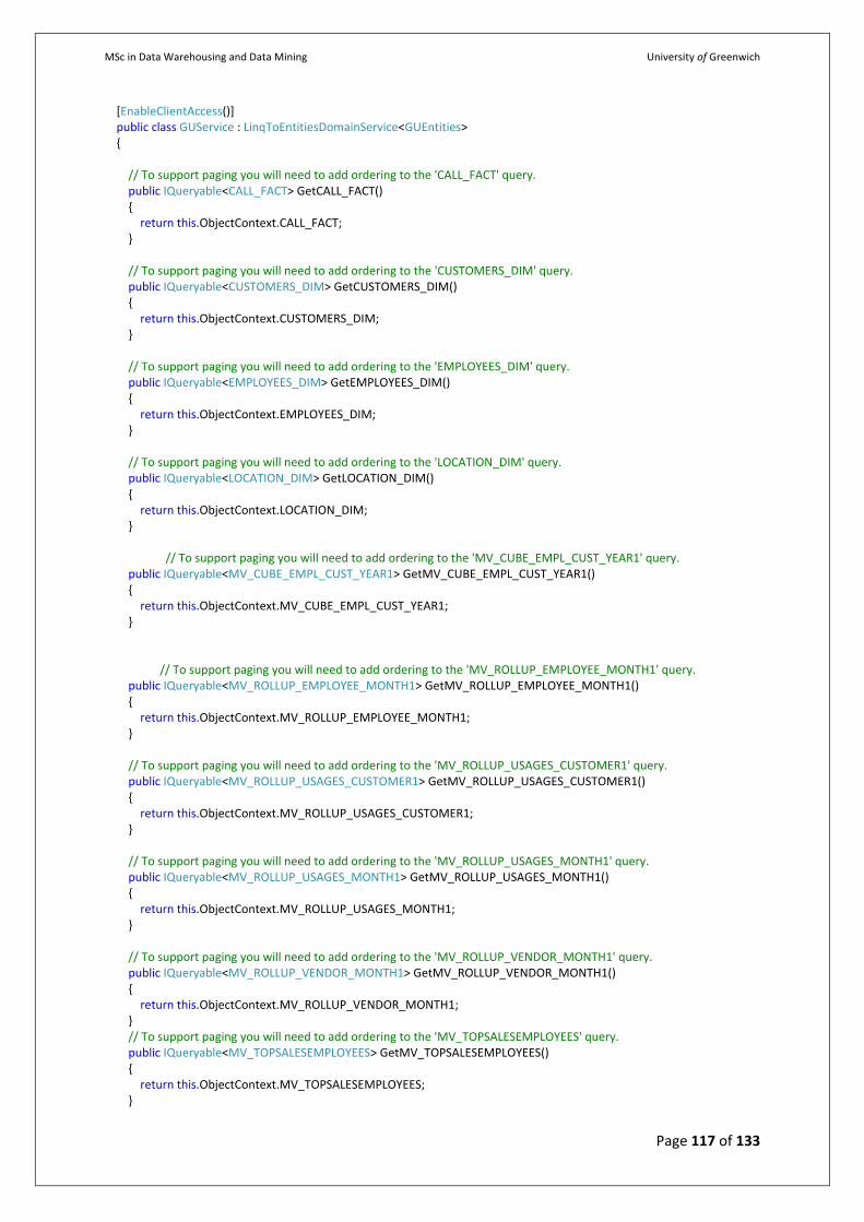
MSc in Data Warehousing and Data Mining University of Greenwich
Page 117 of 133
[EnableClientAccess()] public class GUService : LinqToEntitiesDomainService<GUEntities> { // To support paging you will need to add ordering to the 'CALL_FACT' query. public IQueryable<CALL_FACT> GetCALL_FACT() { return this.ObjectContext.CALL_FACT; } // To support paging you will need to add ordering to the 'CUSTOMERS_DIM' query. public IQueryable<CUSTOMERS_DIM> GetCUSTOMERS_DIM() { return this.ObjectContext.CUSTOMERS_DIM; } // To support paging you will need to add ordering to the 'EMPLOYEES_DIM' query. public IQueryable<EMPLOYEES_DIM> GetEMPLOYEES_DIM() { return this.ObjectContext.EMPLOYEES_DIM; } // To support paging you will need to add ordering to the 'LOCATION_DIM' query. public IQueryable<LOCATION_DIM> GetLOCATION_DIM() { return this.ObjectContext.LOCATION_DIM; }
// To support paging you will need to add ordering to the 'MV_CUBE_EMPL_CUST_YEAR1' query. public IQueryable<MV_CUBE_EMPL_CUST_YEAR1> GetMV_CUBE_EMPL_CUST_YEAR1() { return this.ObjectContext.MV_CUBE_EMPL_CUST_YEAR1; }
// To support paging you will need to add ordering to the 'MV_ROLLUP_EMPLOYEE_MONTH1' query. public IQueryable<MV_ROLLUP_EMPLOYEE_MONTH1> GetMV_ROLLUP_EMPLOYEE_MONTH1() { return this.ObjectContext.MV_ROLLUP_EMPLOYEE_MONTH1; } // To support paging you will need to add ordering to the 'MV_ROLLUP_USAGES_CUSTOMER1' query. public IQueryable<MV_ROLLUP_USAGES_CUSTOMER1> GetMV_ROLLUP_USAGES_CUSTOMER1() { return this.ObjectContext.MV_ROLLUP_USAGES_CUSTOMER1; } // To support paging you will need to add ordering to the 'MV_ROLLUP_USAGES_MONTH1' query. public IQueryable<MV_ROLLUP_USAGES_MONTH1> GetMV_ROLLUP_USAGES_MONTH1() { return this.ObjectContext.MV_ROLLUP_USAGES_MONTH1; } // To support paging you will need to add ordering to the 'MV_ROLLUP_VENDOR_MONTH1' query. public IQueryable<MV_ROLLUP_VENDOR_MONTH1> GetMV_ROLLUP_VENDOR_MONTH1() { return this.ObjectContext.MV_ROLLUP_VENDOR_MONTH1; } // To support paging you will need to add ordering to the 'MV_TOPSALESEMPLOYEES' query. public IQueryable<MV_TOPSALESEMPLOYEES> GetMV_TOPSALESEMPLOYEES() { return this.ObjectContext.MV_TOPSALESEMPLOYEES; }
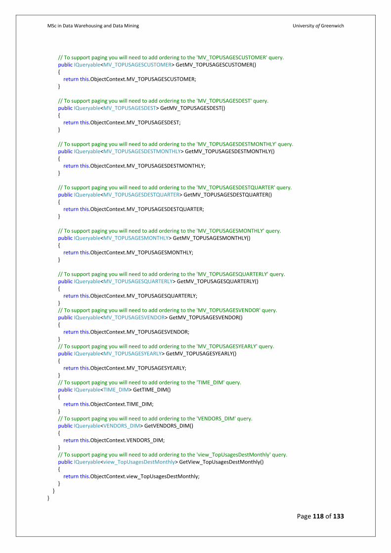
MSc in Data Warehousing and Data Mining University of Greenwich
Page 118 of 133
// To support paging you will need to add ordering to the 'MV_TOPUSAGESCUSTOMER' query. public IQueryable<MV_TOPUSAGESCUSTOMER> GetMV_TOPUSAGESCUSTOMER() { return this.ObjectContext.MV_TOPUSAGESCUSTOMER; } // To support paging you will need to add ordering to the 'MV_TOPUSAGESDEST' query. public IQueryable<MV_TOPUSAGESDEST> GetMV_TOPUSAGESDEST() { return this.ObjectContext.MV_TOPUSAGESDEST; } // To support paging you will need to add ordering to the 'MV_TOPUSAGESDESTMONTHLY' query. public IQueryable<MV_TOPUSAGESDESTMONTHLY> GetMV_TOPUSAGESDESTMONTHLY() { return this.ObjectContext.MV_TOPUSAGESDESTMONTHLY; } // To support paging you will need to add ordering to the 'MV_TOPUSAGESDESTQUARTER' query. public IQueryable<MV_TOPUSAGESDESTQUARTER> GetMV_TOPUSAGESDESTQUARTER() { return this.ObjectContext.MV_TOPUSAGESDESTQUARTER; } // To support paging you will need to add ordering to the 'MV_TOPUSAGESMONTHLY' query. public IQueryable<MV_TOPUSAGESMONTHLY> GetMV_TOPUSAGESMONTHLY() { return this.ObjectContext.MV_TOPUSAGESMONTHLY; } // To support paging you will need to add ordering to the 'MV_TOPUSAGESQUARTERLY' query. public IQueryable<MV_TOPUSAGESQUARTERLY> GetMV_TOPUSAGESQUARTERLY() { return this.ObjectContext.MV_TOPUSAGESQUARTERLY; } // To support paging you will need to add ordering to the 'MV_TOPUSAGESVENDOR' query. public IQueryable<MV_TOPUSAGESVENDOR> GetMV_TOPUSAGESVENDOR() { return this.ObjectContext.MV_TOPUSAGESVENDOR; } // To support paging you will need to add ordering to the 'MV_TOPUSAGESYEARLY' query. public IQueryable<MV_TOPUSAGESYEARLY> GetMV_TOPUSAGESYEARLY() { return this.ObjectContext.MV_TOPUSAGESYEARLY; } // To support paging you will need to add ordering to the 'TIME_DIM' query. public IQueryable<TIME_DIM> GetTIME_DIM() { return this.ObjectContext.TIME_DIM; } // To support paging you will need to add ordering to the 'VENDORS_DIM' query. public IQueryable<VENDORS_DIM> GetVENDORS_DIM() { return this.ObjectContext.VENDORS_DIM; } // To support paging you will need to add ordering to the 'view_TopUsagesDestMonthly' query. public IQueryable<view_TopUsagesDestMonthly> GetView_TopUsagesDestMonthly() { return this.ObjectContext.view_TopUsagesDestMonthly; } } }
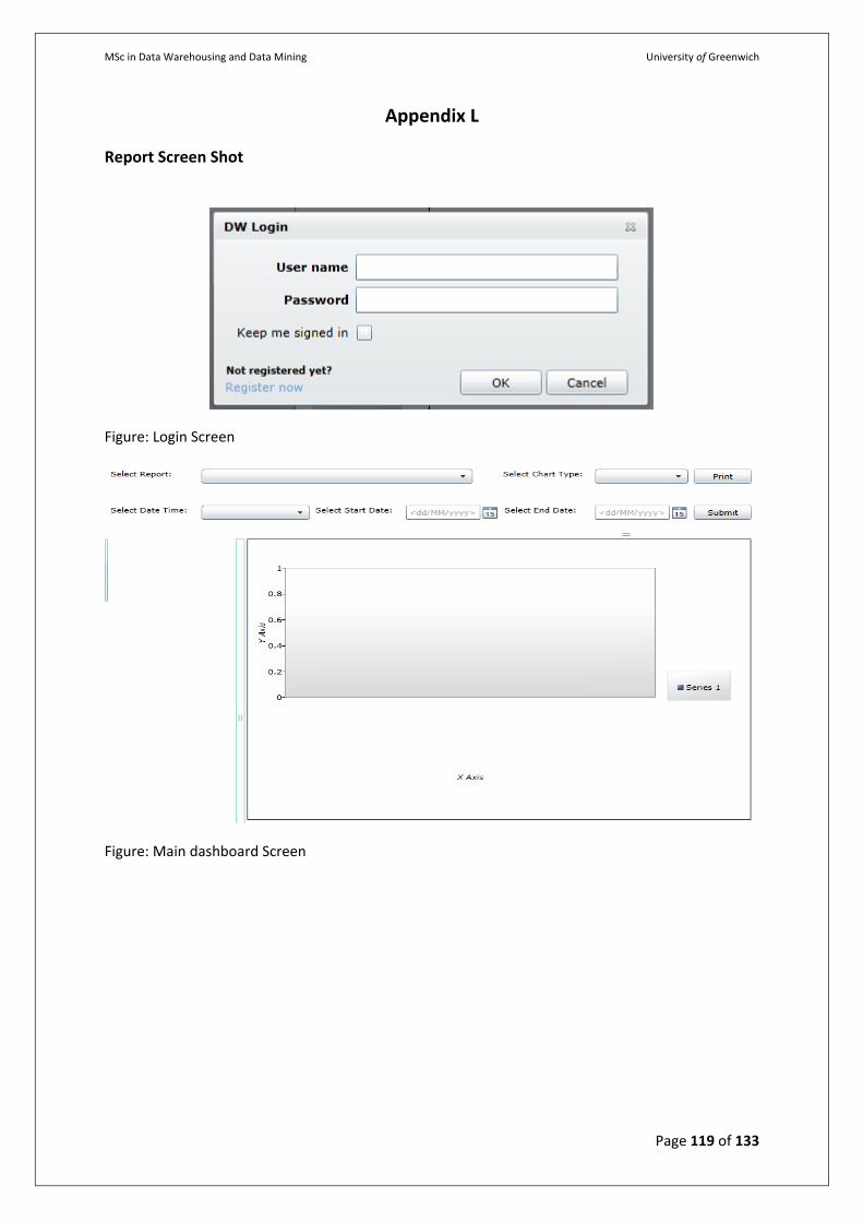
MSc in Data Warehousing and Data Mining University of Greenwich
Page 119 of 133
Appendix L
Report Screen Shot
Figure: Login Screen
Figure: Main dashboard Screen
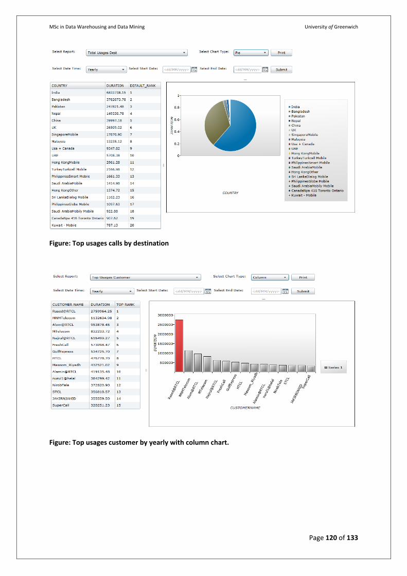
MSc in Data Warehousing and Data Mining University of Greenwich
Page 120 of 133
Figure: Top usages calls by destination
Figure: Top usages customer by yearly with column chart.
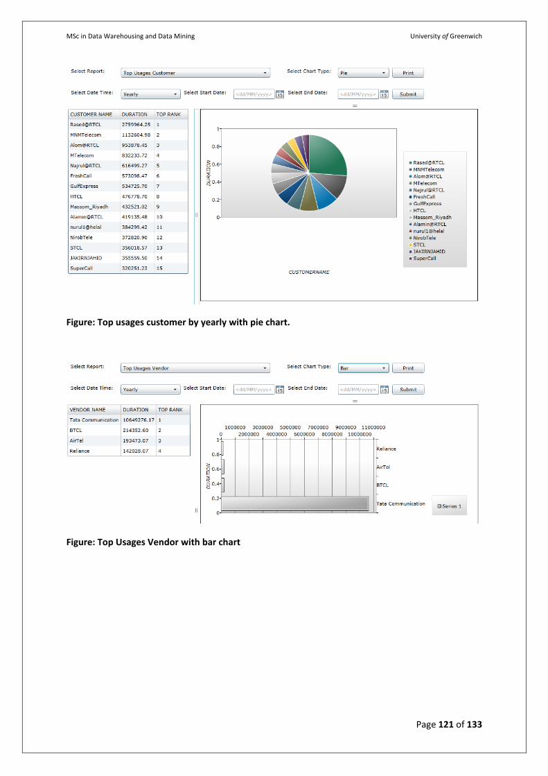
MSc in Data Warehousing and Data Mining University of Greenwich
Page 121 of 133
Figure: Top usages customer by yearly with pie chart.
Figure: Top Usages Vendor with bar chart
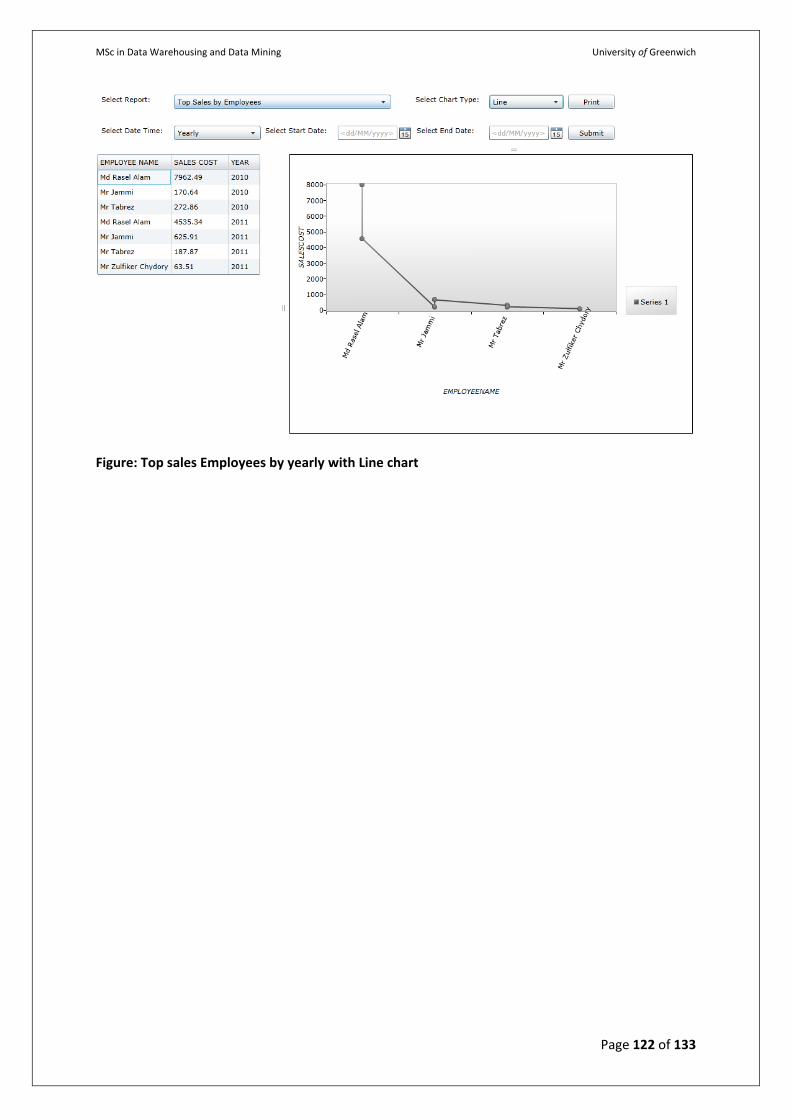
MSc in Data Warehousing and Data Mining University of Greenwich
Page 122 of 133
Figure: Top sales Employees by yearly with Line chart
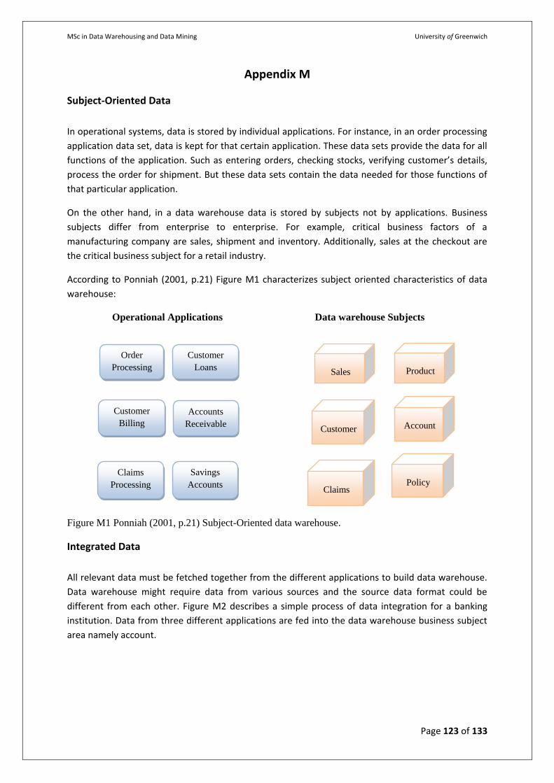
MSc in Data Warehousing and Data Mining University of Greenwich
Page 123 of 133
Appendix M
Subject-Oriented Data
In operational systems, data is stored by individual applications. For instance, in an order processing
application data set, data is kept for that certain application. These data sets provide the data for all
functions of the application. Such as entering orders, checking stocks, verifying customer’s details,
process the order for shipment. But these data sets contain the data needed for those functions of
that particular application.
On the other hand, in a data warehouse data is stored by subjects not by applications. Business
subjects differ from enterprise to enterprise. For example, critical business factors of a
manufacturing company are sales, shipment and inventory. Additionally, sales at the checkout are
the critical business subject for a retail industry.
According to Ponniah (2001, p.21) Figure M1 characterizes subject oriented characteristics of data
warehouse:
Operational Applications Data warehouse Subjects
Figure M1 Ponniah (2001, p.21) Subject-Oriented data warehouse.
Integrated Data
All relevant data must be fetched together from the different applications to build data warehouse.
Data warehouse might require data from various sources and the source data format could be
different from each other. Figure M2 describes a simple process of data integration for a banking
institution. Data from three different applications are fed into the data warehouse business subject
area namely account.
Order
Processing
Customer
Billing
Claims
Processing
Customer
Loans
Accounts
Receivable
Savings
Accounts
Sales
Customer
Account
Policy
Claims
Product
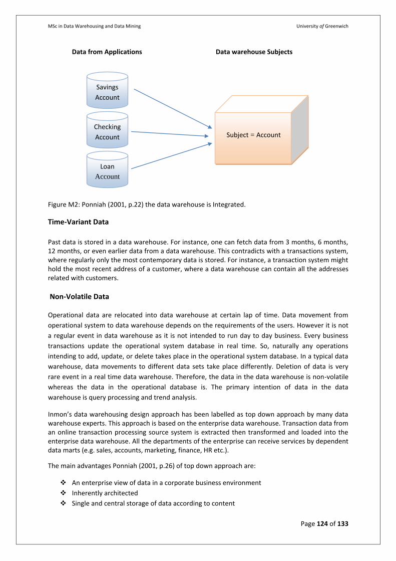
MSc in Data Warehousing and Data Mining University of Greenwich
Page 124 of 133
Data from Applications Data warehouse Subjects
Figure M2: Ponniah (2001, p.22) the data warehouse is Integrated.
Time-Variant Data
Past data is stored in a data warehouse. For instance, one can fetch data from 3 months, 6 months, 12 months, or even earlier data from a data warehouse. This contradicts with a transactions system, where regularly only the most contemporary data is stored. For instance, a transaction system might hold the most recent address of a customer, where a data warehouse can contain all the addresses related with customers.
Non-Volatile Data
Operational data are relocated into data warehouse at certain lap of time. Data movement from
operational system to data warehouse depends on the requirements of the users. However it is not
a regular event in data warehouse as it is not intended to run day to day business. Every business
transactions update the operational system database in real time. So, naturally any operations
intending to add, update, or delete takes place in the operational system database. In a typical data
warehouse, data movements to different data sets take place differently. Deletion of data is very
rare event in a real time data warehouse. Therefore, the data in the data warehouse is non-volatile
whereas the data in the operational database is. The primary intention of data in the data
warehouse is query processing and trend analysis.
Inmon’s data warehousing design approach has been labelled as top down approach by many data warehouse experts. This approach is based on the enterprise data warehouse. Transaction data from an online transaction processing source system is extracted then transformed and loaded into the enterprise data warehouse. All the departments of the enterprise can receive services by dependent data marts (e.g. sales, accounts, marketing, finance, HR etc.).
The main advantages Ponniah (2001, p.26) of top down approach are:
An enterprise view of data in a corporate business environment
Inherently architected
Single and central storage of data according to content
Savings
Account
Checking
Account
Loan
Account
Subject = Account
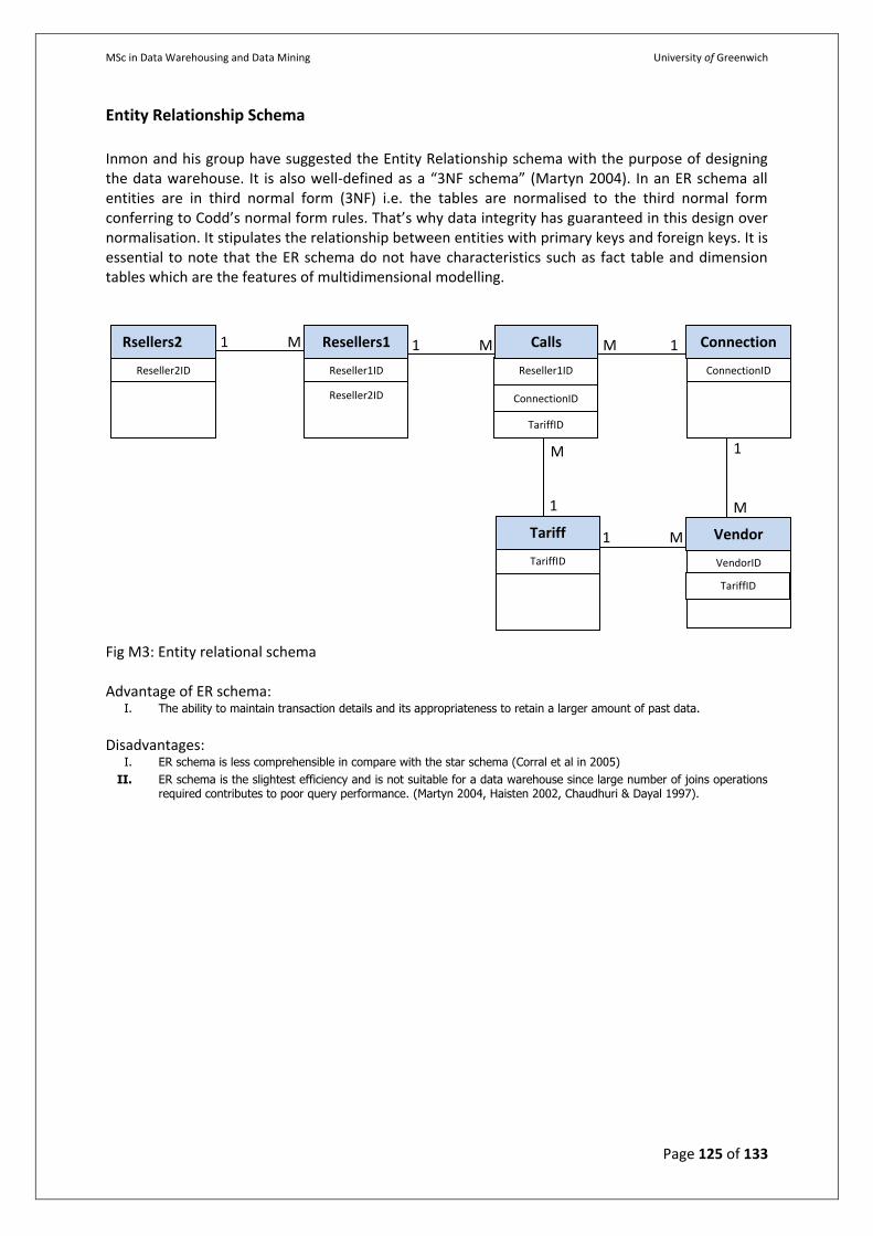
MSc in Data Warehousing and Data Mining University of Greenwich
Page 125 of 133
Entity Relationship Schema
Inmon and his group have suggested the Entity Relationship schema with the purpose of designing the data warehouse. It is also well-defined as a “3NF schema” (Martyn 2004). In an ER schema all entities are in third normal form (3NF) i.e. the tables are normalised to the third normal form conferring to Codd’s normal form rules. That’s why data integrity has guaranteed in this design over normalisation. It stipulates the relationship between entities with primary keys and foreign keys. It is essential to note that the ER schema do not have characteristics such as fact table and dimension tables which are the features of multidimensional modelling. Fig M3: Entity relational schema Advantage of ER schema:
I. The ability to maintain transaction details and its appropriateness to retain a larger amount of past data.
Disadvantages:
I. ER schema is less comprehensible in compare with the star schema (Corral et al in 2005)
II. ER schema is the slightest efficiency and is not suitable for a data warehouse since large number of joins operations required contributes to poor query performance. (Martyn 2004, Haisten 2002, Chaudhuri & Dayal 1997).
M
1
1
M
M 1
1 M M 1 M 1
Reseller2ID
Rsellers2
Reseller1ID
Reseller2ID
Resellers1
Reseller1ID
Calls
ConnectionID
Connection
TariffID
Tariff
VendorID
Vendor
ConnectionID
TariffID
TariffID