Embed Size (px)
Citation preview
Brigham Young University Brigham Young University
BYU ScholarsArchive BYU ScholarsArchive
Theses and Dissertations
2015-03-01
The Programmatic Generation of Discrete-Event Simulation The Programmatic Generation of Discrete-Event Simulation
Models from Production Tracking Data Models from Production Tracking Data
Christopher Rand Smith Brigham Young University - Provo
Follow this and additional works at: https://scholarsarchive.byu.edu/etd
Part of the Industrial Technology Commons
BYU ScholarsArchive Citation BYU ScholarsArchive Citation Smith, Christopher Rand, "The Programmatic Generation of Discrete-Event Simulation Models from Production Tracking Data" (2015). Theses and Dissertations. 5829. https://scholarsarchive.byu.edu/etd/5829
This Thesis is brought to you for free and open access by BYU ScholarsArchive. It has been accepted for inclusion in Theses and Dissertations by an authorized administrator of BYU ScholarsArchive. For more information, please contact [email protected], [email protected].

The Programmatic Generation of Discrete-Event
Simulation Models from Production
Tracking Data
Christopher Rand Smith
A thesis submitted to the faculty of Brigham Young University
in partial fulfillment of the requirements for the degree of
Master of Science
Charles R. Harrell, Chair Michael P. Miles
Andrew R. George
School of Technology
Brigham Young University
March 2015
Copyright © 2015 Christopher Rand Smith
All Rights Reserved
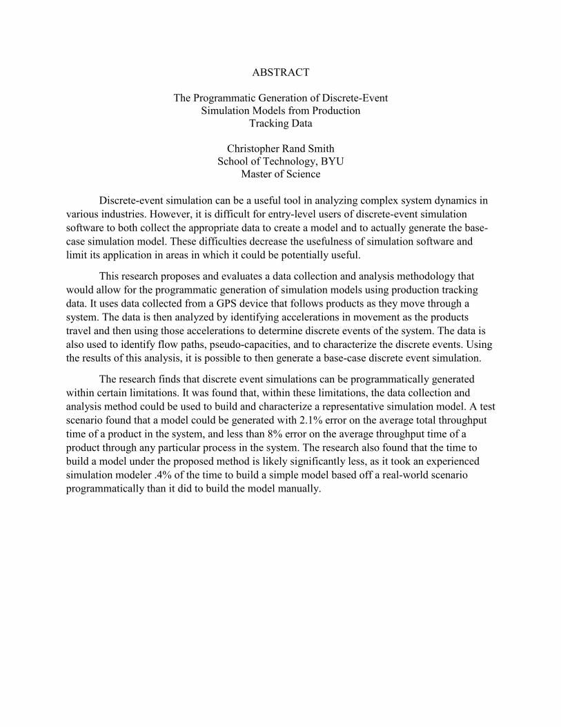
ABSTRACT
The Programmatic Generation of Discrete-Event Simulation Models from Production
Tracking Data
Christopher Rand Smith School of Technology, BYU
Master of Science
Discrete-event simulation can be a useful tool in analyzing complex system dynamics in various industries. However, it is difficult for entry-level users of discrete-event simulation software to both collect the appropriate data to create a model and to actually generate the base-case simulation model. These difficulties decrease the usefulness of simulation software and limit its application in areas in which it could be potentially useful.
This research proposes and evaluates a data collection and analysis methodology that would allow for the programmatic generation of simulation models using production tracking data. It uses data collected from a GPS device that follows products as they move through a system. The data is then analyzed by identifying accelerations in movement as the products travel and then using those accelerations to determine discrete events of the system. The data is also used to identify flow paths, pseudo-capacities, and to characterize the discrete events. Using the results of this analysis, it is possible to then generate a base-case discrete event simulation.
The research finds that discrete event simulations can be programmatically generated within certain limitations. It was found that, within these limitations, the data collection and analysis method could be used to build and characterize a representative simulation model. A test scenario found that a model could be generated with 2.1% error on the average total throughput time of a product in the system, and less than 8% error on the average throughput time of a product through any particular process in the system. The research also found that the time to build a model under the proposed method is likely significantly less, as it took an experienced simulation modeler .4% of the time to build a simple model based off a real-world scenario programmatically than it did to build the model manually.

ACKNOWLEDGEMENTS
Many thanks to my wife, Stephanie, for her help, patience, and consistent encouragement
throughout. My family, most particularly parents, grandparents, siblings, in-laws, and all others,
also deserve my sincere gratitude for their support and encouragement. In addition, I would like
to thank my committee for their help and support.

TABLE OF CONTENTS
ABSTRACT ................................................................................................................................... ii
LIST OF TABLES ...................................................................................................................... vii
LIST OF FIGURES ................................................................................................................... viii
1 Introduction ........................................................................................................................... 1
1.1 Background ..................................................................................................................... 1
1.2 Objective ......................................................................................................................... 2
1.3 Justification ..................................................................................................................... 2
1.4 Limitations ...................................................................................................................... 3
1.5 Glossary of Terms ........................................................................................................... 4
2 Literature Review ................................................................................................................. 5
2.1 Problem Definition ......................................................................................................... 5
2.2 Programmatic Model Generation .................................................................................... 6
2.3 Data Collection for Simulation Models .......................................................................... 6
2.4 Creating Models from GPS Data .................................................................................... 6
2.5 GPS Accuracy ................................................................................................................. 8
2.6 Multi-Resolution Modeling .......................................................................................... 10
3 Methodology ........................................................................................................................ 11
3.1 Introduction ................................................................................................................... 11
3.2 Development of Model Creation Algorithm ................................................................. 11
3.3 Development of Data Collection System ...................................................................... 12
3.4 Scenario Testing ........................................................................................................... 14
4 Results and Analysis ........................................................................................................... 16
4.1 Data Analysis Algorithm .............................................................................................. 16 iv

4.1.1 Identifying Process Steps .......................................................................................... 16
4.1.2 Characterizing Process Steps .................................................................................... 19
4.1.3 Identifying Product Flow .......................................................................................... 20
4.1.4 Algorithm Output Capability .................................................................................... 22
4.2 Data Gathering Tool Variation ..................................................................................... 24
4.3 Scenario 1 - Car Route .................................................................................................. 25
4.3.1 Scenario 2 - Walking Route ...................................................................................... 26
4.3.2 Limitations of Data Gathering Tool .......................................................................... 26
4.4 Programmatically Generated Model Accuracy ............................................................. 28
4.4.1 Generated Simulation ................................................................................................ 29
4.4.2 Scenario 1 - Car Route .............................................................................................. 31
4.4.3 Scenario 2 - Walking Route ...................................................................................... 33
4.5 Capability of Proposed Model-Building Methodology ................................................ 34
4.6 Time-Savings of Proposed Model-Building Methodology .......................................... 35
5 Conclusions .......................................................................................................................... 36
5.1 Limitations of Algorithm .............................................................................................. 36
5.1.1 Algorithmic Limitations ............................................................................................ 37
5.1.2 Methodical Limitations ............................................................................................. 39
5.2 Summary ....................................................................................................................... 41
References .................................................................................................................................... 43
Appendix A. Data Collection Tool Code ................................................................................ 45
A.1. Code - Location.php ........................................................................................................ 45
Appendix B. Data Analysis Algorithm Tool Code ................................................................ 47
B.1. Code - DataAnalysis Module .......................................................................................... 47
v
B.2. Code - Settings Form ...................................................................................................... 58
B.3. Code - Distribution-Fitting.php ....................................................................................... 59
Appendix C. FlexSim Data Translator Code ........................................................................ 61
C.1. Code - FlexSim Function: ModelImport ......................................................................... 61
C.2. Code - FlexSim Function: FivePointDistribution ........................................................... 65
Appendix D. Five-Point Distribution ..................................................................................... 66
D.1. Explanation ..................................................................................................................... 66
vi

LIST OF TABLES
Table 3-1: Example of Data Gathering Tool Output .................................................................... 13
Table 4-1: Output of the Data Analysis Algorithm from the Car Route Scenario ....................... 22
Table 4-2: Algorithm Output Usage in Model Input .................................................................... 23
Table 4-3: Error of Characteristics of Programmatically Generated Model ................................. 29
Table 4-4: Characteristics of Manually Generated Original Model ............................................. 29
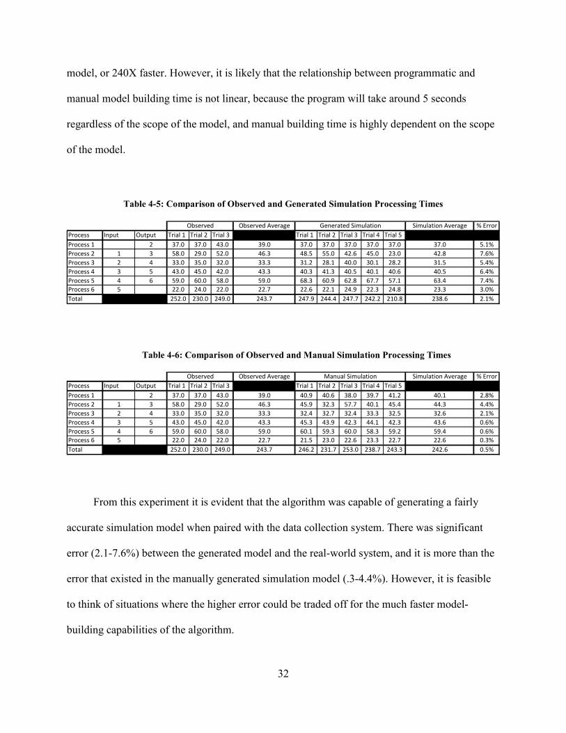
Table 4-5: Comparison of Observed and Generated Simulation Processing Times ..................... 32
Table 4-6: Comparison of Observed and Manual Simulation Processing Times ......................... 32
Table 4-7: Characteristics of Walking Route System. .................................................................. 33
vii

LIST OF FIGURES
Figure 4-1: Acceleration in Time of a Product and Cutoff Point ................................................. 17
Figure 4-2: Scatterplot of Coordinate Locations During Trial 1 .................................................. 25
Figure 4-3: Original (Top) and Programmatically Generated (Bottom) Simulations................... 30
Figure 4-4: Position of Data Points in Scenario 2 Trials .............................................................. 33
viii

1 INTRODUCTION
1.1 Background
Discrete-event simulation software has proven to be a reliable tool for system
improvement, because it is able to assist a user in identifying and solving problems. An accurate
simulation model also gives the user an opportunity to explore a defined system or test “what-if”
scenarios without having to invest the time and money that would be necessary to test out
different scenarios on the actual system. These benefits are infrequently realized in industry,
because entry-level users of discrete-event simulation software find it difficult to gather the data
necessary to create a simulation and also have difficulty using correctly gathered data to create a
base case scenario. Without the base-case scenario it is difficult to explore the system or test
“what-if” scenarios using simulation.
However, if discrete-event simulation software were able to reduce the amount of
training, experience, and time necessary to create accurate simulation models, then a discrete-
event simulation tool would be useful for a larger subset of people. The use of discrete-event
simulation tools would likely increase due to the more favorable balance between the time
invested in creating the model and the benefits of the insight gained from the model.
1
1.2 Objective
The purpose of this thesis is to develop methods for collecting and analyzing product
location data as it moves through production in order to programmatically create discrete-event
simulation models. The research answers the following questions:
1. Can timestamp and location data collected through a GPS tracker be used to facilitate
programmatic model creation?
2. Can programmatic model creation tools be used to facilitate model creation in a way
that product flow and processing is determined through analysis of a sample of
product location data as it moves through a system?
3. Can the lead time required to create an accurate simulation model be reduced by
using automated data collection and programmatic model creation?
4. What types of data are ignored or unachievable through this form of analysis?
1.3 Justification
The following two problems are currently experienced by users that are beginning to use
discrete-event simulation software:
1. The data collection phase of a project does not always occur in the same time period
as model creation, which often results in inaccurate model results.
2. The user experiences a high lead time from the start of model creation to getting
results of simulated what-if scenarios.
2
Currently discrete-event simulation software has a steep learning curve, which
necessitates large amounts of training and/or expertise in order to produce models that can
accurately depict the real-world scenario that is being simulated. Over the years many changes
have been made in various discrete-event simulation software packages to try to reduce the
learning curve, and enhance the ability of an entry-level user. These changes have managed to
decrease the amount of coding experience and other skills necessary to model common
scenarios. However, many entry-level users of discrete-event simulation software still become
discouraged by the amount of training, experience, and, most importantly, time that is necessary
to achieve worthwhile simulation results. By supplying a possible solution to this difficulty the
usefulness of simulation software can be enhanced. However, this research does not presume that
training and experience will no longer be useful, as any significant modifications of the base case
will have to be done by a more experienced modeler.
1.4 Limitations
This research is limited to the scope of systems where the products physically move
through a set of processes. It also does not attempt to include in the generated simulations the
actions of indirect resources on the product. Therefore, this method would be ineffective in
instances where indirect resource capability is the main objective of simulation, and would be
more effective where throughput and bottleneck analysis is the desired result of simulation. For
additional limitations of method see section 5.3 Limitations of Algorithm.
3
1.5 Glossary of Terms
Computer Simulation: A computer model that is made to represent or mimic an actual
system. The model is then used to draw inferences on the behavior of the actual system.
Discrete-Event Simulation (DES): A subset of computer simulation that is involved in
modeling systems where events drive the system. This is in contrast to other forms of computer
simulation including fluid simulation, stress simulation, and others where events do not drive the
simulation.
Processor: A step in a system in which the product is contained for a determined interval
of time. This step differs from a queue, because although the interval of time may be non-
constant it is not considered waiting time. Movement of an item between system steps is also
modeled as a processor in this research.
Product: The item that moves through the system. This is the part of the system in the
research that is tracked using a GPS tracking system.
Queue: A step in the system where the time can be classified as waiting time. The
waiting time could be determined be either a downstream or upstream process.
Route: The specific series of processors and queues that the product moves through in
the system. The route can be constant or variable. Different products may experience different
routes or routing as they move through the system.
System: The aggregate of all non-product items making up a model.
4

2 LITERATURE REVIEW
2.1 Problem Definition
There is an abundance of articles both within academia and from without that highlight
the problem that is being addressed by this thesis. A particularly good article highlights the
amount of time in a simulation model that is spent collecting, analyzing, and inputting data into
the simulation model (Skoogh, 2012). This article makes the following noteworthy observation:
However, despite its potential, industries worldwide have not adopted DES completely in their production development process. One reason is arguably that production simulation projects tend to be slow in providing clients with model results. This is a significant disadvantage, since manufacturing development and design projects usually rely on rapid responses from analyses. Hence, renouncing precision in favor of quick response, organizations are tempted to choose less complex tools. (Skoogh, 2012)
This observation is helpful in defining the problem that DES is currently experiencing. The lead
time between starting the analysis and getting results seems to be prohibitively long for many
potential users. This article also mentions that “activities in the input data management process
constitute around one third of the total time consumption in DES projects.” This is important,
because the proposed data collection and analysis portion of this research aims to reduce both
that time and the model creation time in the total time of a DES project. It is clear that a problem
currently exists, because of the long lead time in DES projects. It is also clear that resolving this
problem could lead to DES being used more frequently as a tool.
5
2.2 Programmatic Model Generation
Programmatic model generation is a topic that has been explored in a variety of other
articles. One article, “Stochastic generation of discrete-event simulation models,” identifies the
different steps that are necessary in creating models (Huber, 2008). These steps are identified as
the following: definition of input parameters, model hierarchy creation, component placement,
component linkage, and variable variation. This research attempts to programmatically
accomplish each of the steps as outlined in this previous research. For similar research that has
been done to programmatically create models for forms of data analysis other than simulation see
Section 2.4 Creating Models from GPS Data.
2.3 Data Collection for Simulation Models
Many articles have identified data collections methods for the successful creation of
statistically representative simulation models. An article, “Automated input data management:
Evaluation of a concept for reduced time consumption in discrete event simulation,” proposes an
idea that attempts to reduce the amount of time that is necessary for data input in creating a
simulation model (Skoogh, 2012). The idea presented is a complicated system that allows for
real-time simulation updates. The system derived in this research accomplishes a similar goal to
the solution that will be proposed, but seems to do it in a much more intrusive manner to an
operation than would be feasible in many manufacturing environments.
2.4 Creating Models from GPS Data
There are a few articles of research that have used GPS data to create models of real-
world scenarios, but they were not creating discrete-event simulations. Most of these articles
6

dealt with analyzing traffic flow patterns, and creating models of traffic networks.
Programmatically modelling traffic networks actually has many similarities to programmatically
generating discrete-event simulations, because they both must identify when events happen, how
long they take, and how objects move between those events. There were a couple interesting
articles that attempted to use GPS data to create models of traffic flow.
One article was using GPS data to try to identify the most efficient traffic route and then
compared that route to those that people chose manually (Spissu, 2011). This article establishes
some of the difficulties with using GPS data from the modelling of routes. It found the
following:
Although GPS-based data collection and, in particular, smart phone data collection have been shown to offer a number of advantages in the present and earlier studies, some technological limitations still affect data quality. In this work, 42% of the reported trips could not be associated with the corresponding routes mostly because of canyon effects, signal reflex, and user carelessness. (Spissu, 2011)
The findings from that article make it clear that care must be taken when using GPS to ensure
that data is collected in areas where its limitations can be reduced.
Another article was attempting to estimate travel time of routes through an arterial
network of roadways (Pan, 2007). The difficulty with this task is that arterial roadways have
many stops signs, stop lights, and congestion that makes classifying that time difficult. The
planned stoppages (i.e. stop signs and stop lights) were classified in the research as links. The
method of the research was to use continuously sampled GPS data to identify when a vehicle was
decelerating and then attributed any time between that deceleration and the next acceleration to
the closest link (Pan, 2007). That link was then characterized by an average of the experienced
times during the sample. This article proposes some similar concepts to those that are being
presented in the current research, because the current research also uses acceleration to identify
7

when an object is in a new process. The current research then associates the time between that
acceleration and the next acceleration as belonging to the process. This article found that it was
able to determine the link time (the time between when a person started decelerating at a stop
sign or stoplight to when they finished accelerating afterwards) with about 5.5% error using data
collected with a GPS data collection system.
2.5 GPS Accuracy
This research depends on a data collection tool that can provide a coordinate position.
Specifically this research used GPS coordinates to define product movement through a system.
In order to know the limitation of this research it is necessary to know the limitation of the
devices that were used in collecting the data. The tool’s limitations directly influenced the types
of systems that can use the proposed methodology to create a simulation model. The current
accuracy of a worst-case scenario for uncorrected civilian GPS coordinates at a 95% confidence
level is 7.8 meters (Department of Defense, 2008). However, if one uses multiple satellites,
augmentation services, or other correction methods it is realistic to achieve accuracies within a
few centimeters (NGS, 2014). Therefore, it is reasonably possible to use this method on systems
where the significant distance between processes is greater than the limitation of the data
collection tool, which is a few centimeters. Other methods could be used to gather this type of
data including ultrasonic methods, RF mapping, etc., but those methods, due to their less
developed nature, weren’t explored in this research. GPS is especially useful because of the
active development that is occurring in this area. With newer GPS satellites that are currently in
development, it is anticipated that uncorrected civilian GPS accuracy will drop to 0.63 meters
8

(United States Air Force, 2014). The current research used uncorrected GPS coordinates, which
resulted in significant error in scenarios with movement on a small scale.
Various research articles have used a similar GPS data collection method. One such
research article found that a GPS data collection system could be used to adequately gather
location and timestamp data to track the usage of construction equipment on a construction site
(Pradhananga, 2013). That research acknowledged that there are multiple approaches that could
be used to collect location data, and that each has benefits and limitations. However, as it states:
GPS is well known to work independently (defined as a device that may not require any other installation of technology on a project site, other than a device on the resource to track it) and provide real-time data (defined as equal or greater than 1 Hz data update rate)… GPS devices are also affordable and easy to install. The data it provides can also be analyzed with relative little computational effort. For these reasons, this work presents the implementation of GPS technology for tracking the location of construction equipment as it relates to work sampling, including cyclic activities which are very common in earth moving operations. (Pradhananga, 2013)
Similar benefits are recognized in the current research by using GPS instead of other methods for
tracking location. Another finding from that same research was the observed accuracy that was
achieved with low-cost GPS systems, which was 0.68-4.36 meters (Pradhananga, 2013). It found
the following:
In sum, the GPS data loggers were found to perform better under clear view of sky while the performance degraded with increasing obstacles. The standard deviations were high compared to the value of the mean in all cases, indicating that the readings were not consistent and can vary significantly. It should also be noted that error rates vary among data loggers. The above error tests, however, provide a general idea of what data low-cost easy-to-install GPS data can provide. (Pradhananga, 2013)
From this analysis it would seem that either a higher quality GPS device would need to be used in
order to get data using a GPS for a small scale system, or the GPS device would need to be better
than the low-cost option used in the aforementioned research.
9

2.6 Multi-Resolution Modeling
An interesting caveat to this research is the capability to automatically do multi-
resolution simulation modeling. The idea of multi-resolution modeling is presented in the article
“Using dynamic multiresolution modelling to analyze large material flow systems”
(Dangelmaier, 2004). This article introduces the idea of multi-level simulation modeling. It also
presents the idea of model scope indication by view distance in the model. This suggests that
representative simulation models can be achieved by increasing the scope in one area of the
simulation that is crucial to the modeler while decreasing the scope in other areas. This concept
may be a possibility for the simulation models created using the method that are proposed in this
thesis.
10
3 METHODOLOGY
3.1 Introduction
The methodology for developing an algorithm for programmatically generating discrete-
event simulation models from production tracking data was separated into the following three
sequential phases:
Phase 1 – Development of Model Creation Algorithm
Phase 2 – Development of Data Collection System
Phase 3 – Scenario Testing
3.2 Development of Model Creation Algorithm
This phase of research is concerned with being able to replicate a manually generated
simulation model using a programmatic model creation algorithm. For this phase a simple test
case was generated in simulation software. The software used in the research was FlexSim,
which is a discrete-event simulation software provided by FlexSim Software Products, Inc. The
model was a simple system with six processing steps. The model included the following basic
procedures: processing steps, multiple exit locations, route reentry, route consolidation, route
splitting, probabilistic routing, and variable processing times. The model was developed in order
to create data that would be used to try to programmatically mimic the original model. The
11

dataset was created from the model by recording the absolute x, y, and z location to a general
origin and the time of every product in the system for every second that the model ran. The
dataset included data for 100 products as they went through the modeled system. This data was
then saved in .csv format and imported into excel for data analysis.
Once the dataset was gathered from the initial model, an Excel VBA-based algorithm was
written to comb through the data to attempt to identify the original processes and routing. For
more information about the data analysis algorithm see section 4.1 Data Analysis Algorithm.
This algorithm was then capable of identifying the steps in the system, a distribution that
characterized the processing times of each step, the capacity of each step, and the routing
through the system. The model was then analyzed to determine the accuracy of the
programmatically generated model to the original simulation model using some key output
characteristics, which included the average processing times of each processing step in the model
and the average throughput for each step in the model. The results of those comparisons can be
found in section 4.3.1 Generated Simulation. After developing the programmatic model creation
algorithm it was important to determine the limitations of the algorithm. These limitations and
their significance were explored and the results are found in section 5.3 Limitations of
Algorithm. Phase 1 was finished once the algorithm was created and the limitations identified.
3.3 Development of Data Collection System
The data collection system was developed to provide the following information about a
product at a constant interval as it moved through the system:
12

1. Unique Product Identifier – An indexed number for each product observed.
2. Longitude – The longitudinal position of the observed product at a given time.
3. Latitude – The latitudinal position of the observed product at a given time.
4. Product Type Identifier – An indexed number for each product type observed.
5. Timestamp – The time (in seconds) since the beginning of observation
Once this information was collected the longitude and latitude were converted to X and Y
coordinates based off of an origin at the first position of the first observed product. The
calibration time was also removed from the beginning of the dataset. Once these steps were done
this information created a collection of data points that looked similar to the example in Table
3-1.
Item X Y Type Time1 0 0 1 121 1.519118 -1.61331 1 131 3.038236 -3.22662 1 141 1.082859 -6.48886 1 151 -2.39164 -8.1378 1 161 -20.7806 -17.7902 1 171 -35.695 -25.7936 1 181 -62.5246 -33.7249 1 191 -74.4397 -33.6527 1 201 -95.1282 -33.5273 1 211 -103.901 -33.4741 1 221 -115.156 -33.4058 1 231 -115.419 -33.4042 1 24
Table 3-1: Example of Data Gathering Tool Output
13

3.4 Scenario Testing
Scenario testing was done in an attempt to verify the capability of the proposed
methodology. Two scenarios were developed in order to test the data collection system and the
simulation software data translator that was used to build the models from the data analysis
algorithm output.
The first test scenario was done on a large scale by identifying a driving route between
two locations. The route went through stop signs and traffic lights, which broke the route into
multiple steps. The route was driven three times in order to act as three products moving through
the system. The route was done on a large scale in order to determine the accuracy of model
creation where the amount of tool induced variability was minimal. The actual time for each
segment was recorded during each route. The car was also GPS tracked during each route. The
aggregated GPS data was then sent through the programmatic model creation algorithm in order
to create a representative model, and to identify the various segments. The programmatically
identified time for each segment was then compared to the recorded time. The distribution of
average trip times was also compared to the distribution of calculated trip times. The results of
this scenario can be found in section 4.3.2 Scenario 1 – Car Route.
The second scenario that was analyzed was to determine if the GPS data collection
system would be accurate enough in a small production system. This scenario was setup by
creating five production steps in a small room. The products moved through the system
according to an established model. The time spent in each location was determined variably by
predetermined distributions. Once the system was setup, five products were tracked using GPS
as they moved through the system. The aggregated GPS data for the five products was then sent
through the model generation algorithm to create a simulation model to represent the predefined 14

system. The similarity between the programmatically created model and the predefined system
was then analyzed. The analysis of this scenario can be found in section 4.3.3.
15
4 RESULTS AND ANALYSIS
4.1 Data Analysis Algorithm
To convert GPS data to a discrete-event simulation model it is necessary to run the data
through an algorithm that makes calculations and crucial assumptions. The algorithm
calculations can be broken into three major steps, which are the following:
1. Identify the various process steps.
2. Characterize each of the identified steps.
3. Identify the path the products take as they flow through the process.
As the algorithm moves through these calculations it makes many assumptions. Knowing the
implicit assumptions in the calculations is a critical factor in creating an accurate model using the
algorithm described below.
4.1.1 Identifying Process Steps
The first step in the algorithm is to identify the process steps. This is the most robust part
of the model generation algorithm, because it is the one with the least presumptive assumptions.
This step can be broken down into the following minor steps for each observation:
1. Create a chart of the difference in the absolute value of the instantaneous acceleration of
the object as it moves through time.
16
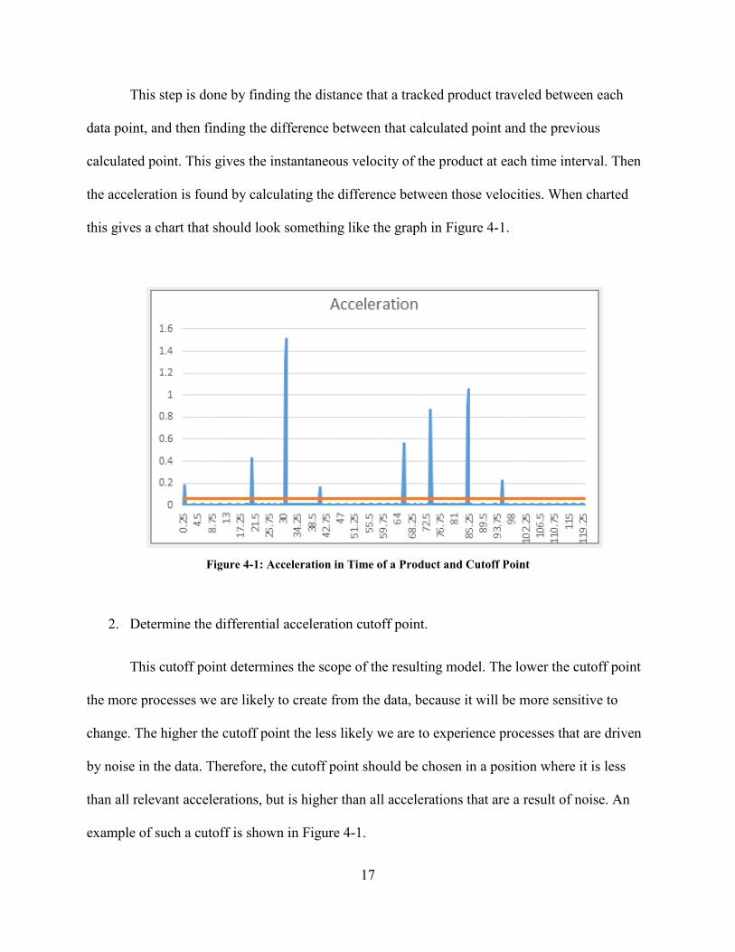
This step is done by finding the distance that a tracked product traveled between each
data point, and then finding the difference between that calculated point and the previous
calculated point. This gives the instantaneous velocity of the product at each time interval. Then
the acceleration is found by calculating the difference between those velocities. When charted
this gives a chart that should look something like the graph in Figure 4-1.
Figure 4-1: Acceleration in Time of a Product and Cutoff Point
2. Determine the differential acceleration cutoff point.
This cutoff point determines the scope of the resulting model. The lower the cutoff point
the more processes we are likely to create from the data, because it will be more sensitive to
change. The higher the cutoff point the less likely we are to experience processes that are driven
by noise in the data. Therefore, the cutoff point should be chosen in a position where it is less
than all relevant accelerations, but is higher than all accelerations that are a result of noise. An
example of such a cutoff is shown in Figure 4-1.
17
3. Determine the location sensitivity measure.
This sensitivity is basically a location sensitivity. A location sensitivity measure must be
used because exactly the same GPS locations are unlikely in simultaneous observations.
Therefore, one must be willing to group processes that start and end in similar areas as the same
process. Therefore, a location setting of one would mean that if a process was found that started
within one distance unit of an existing process, and ended within one distance unit of the same
existing process, then it would be considered the same process.
4. Split each observation into its respective processes using the acceleration cutoff point.
If the acceleration is above the cutoff point, then the points before the cutoff point are
considered a separate process than the points after the cutoff point. For each of the identified
processes calculate a processing time, by subtracting the last time in the process by the first time
in the process. Also determine the process starting point by the first GPS coordinate, and it’s
ending point using the last GPS coordinate.
5. Using the location sensitivity measure, group similar processes between observations.
Use the methods described in detail in the next section, which allow for stochastic
representation of the process.
These steps use the GPS data, and a couple cutoff points to programmatically break the
data into the various processing steps that the product experienced during the observed run.
18
4.1.2 Characterizing Process Steps
The next step in the data analysis algorithm was the need to characterize each of the
process steps that were identified. This process can be done in the following, not necessarily
sequential, steps:
1. Identify a stochastic representation of the processing time for each step
This can be done in a variety of ways. The data could be run through a system that
identifies a distribution with the highest goodness of fit. The distribution could then be sampled
from for the stochastic representation. However, in this research it was instead determined to
generate a stochastic representation whose method could be applied to any situation and
adequately represent the sample. The distribution is described in detail in Appendix D, but it is
basically determined by placing 20% of the area under the probability density curve as a uniform
distribution between the observed minimum and the data point at the 20th percentile of the data.
Then doing likewise for each 20th percentile above that until the last uniform distribution is
located between the 80th percentile of data and the maximum. This distribution does not give a
perfect representation of the data. However, given the other much more important assumptions
used in this generation algorithm this assumption does not seem egregious.
2. Identify if the process is deterministic or indeterministic
The classic examples of both would be a step with a defined process time being
deterministic, and a step that acts as a queue being indeterministic. This research does not
attempt to create a method to identify if a process is deterministic or indeterministic. It assumes
that every process is deterministic. However, this assumption does limit the effectiveness of the
19

algorithm in creating exactly representative simulation models. This step might be achieved by
using the methods explained in section 4.4.1.3. Processing Time vs. Delay Time Identification.
3. Identify a pseudo-capacity of each step
This step can only be done if the sample was taken from sequential products. It is done by
looking at each process step at each unit of time and finding the time unit where the maximum
number of products were in the process step. That maximum can then be considered a pseudo-
capacity of that step in the system. This method is extremely limited, because it is only an
estimated capacity based off of observation, and not necessarily the true limit of the particular
step’s capability. A true capacity would reflect how many units a step could handle in isolation,
however this method creates a capacity that only reflects the experienced maximum in the
sample, and not a true maximum. This method will underestimate the true capacity of any step
where it’s capacity is being limited by another step in the system. Therefore, if capacity
considerations are an important in the desired outcome of the model it would be prudent to adjust
the capacities of the steps of the generated model to more accurately reflect the observed real-
world scenario.
4.1.3 Identifying Product Flow
The next step in the data analysis algorithm is creating the flow by which the products
move through the process steps of the system. This is done by accomplishing the following two
tasks:
20

1. Identify the flow paths
To identify the flow paths it is necessary to recognize the path that each observed product
experienced as it moved through the system. The method to determine paths is to create a list of
the orders a product went through. Once this list is generated for each product we can then make
sure to send the simulation program the necessary information to make the connections between
those events. The output shown in Table 4-1 does this in the columns labeled “IN” and “OUT”.
2. Characterize the flow paths
This is the more difficult of the two tasks associated with creating the flow paths. This
step attempts to identify the logic by which a product decides which step to move to when there
are multiple options. This is not an issue when one step moves to only one other step. But in
other situations, such as which step to proceed to in a situation where one step can go to multiple
other steps, the characterizing of the logic associated with that particular flow is important in
order to accurately reflect the real-world scenario. In order to simplify the model generation
algorithm it was assumed that the generated models relied on probabilistic routing. In other
words it was assumed that, in a situation where a split in routing occurred after a step, a defined
percentage went down each route. If this algorithm was used on a system with multiple product
types, then each product type’s flow would be generated independently. This would be done by
creating probabilistic routing for each case. The algorithm would then be able to split routing by
product type by sending 100% of a theoretical product type 1 to one step and 100% of a
theoretical product type 2 to another step. The assumption of probabilistic routing allows us to
analyze the data by looking at every time an observation left a particular step and then develop a
percentage from the results of where the observations ended up going. This method is not
complete as a lot of routing is not done in a probabilistic manner. However, one could develop 21

methods to identify various other types of routing such as first available or round-robin (see
section 5.3.1.2. Probabilistic Flow).
4.1.4 Algorithm Output Capability
Using the methods in the algorithm it is possible to generate an output that looks
something like Table 4-1. Table 4-1 is the output generated for the car route scenario (see
Section 4.3.2).
Table 4-1: Output of the Data Analysis Algorithm from the Car Route Scenario
The simulation software package is then required to have a translator that takes these simulation
outputs and programmatically create the steps and flow for the model (see Table 4-2).
Process Start X End X Start Y End Y Angle Length IN OUT Times Distributions Pseudo-Capacity0 0 -145.78 0 325.3091 114.1385 356.4799 test|-1`1 37~37~48 fivepointdistribution(37~37~37~39.2~43.6~48) 31 -146.535 74.68844 371.9068 694.5784 55.56544 391.225 test|0`0.6667 12~31 fivepointdistribution(12~15.8~19.6~23.4~27.2~31) 22 131.5003 857.4866 700.4009 698.6524 -0.13799 725.9884 test|1`1 45~15 fivepointdistribution(15~21~27~33~39~45) 23 930.8949 1321.835 696.8568 695.7362 -0.16423 390.9417 test|2`1~13`1 8~9~8 fivepointdistribution(8~8~8~8~8.4~9) 24 1396.76 1765.415 695.787 689.7104 -0.94433 368.7053 test|3`0.6666 8~12 fivepointdistribution(8~8.8~9.6~10.4~11.2~12) 25 1839.646 2203.096 688.7353 680.8994 -1.23508 363.5344 test|4`0.5 8 fivepointdistribution(8~8~8~8~8~8) 16 2255.831 2648.232 679.9061 669.3899 -1.53513 392.542 test|5`1~4`0.5 10~15 fivepointdistribution(10~11~12~13~14~15) 27 2683.38 2746.572 667.9305 39.19389 -84.2607 631.9042 test|6`1~14`1 20~18~18 fivepointdistribution(18~18~18~18.4~19.2~20) 28 2746.214 2744.277 -20.1294 -950.257 269.8807 930.1292 test|7`0.6667 22~23 fivepointdistribution(22~22.2~22.4~22.6~22.8~23) 19 2744.241 2368.044 -976.235 -1047.52 190.7297 382.8907 test|8`1~16`1 15~18~20 fivepointdistribution(15~16.2~17.4~18.4~19.2~20) 2
10 2336.078 1072.152 -1047.12 -1037.96 179.5844 1263.959 test|9`1 29~27~15 fivepointdistribution(15~19.8~24.6~27.4~28.2~29) 211 1009.297 352.4403 -1036.97 -1041.03 180.3541 656.8693 test|10`1 16~19~22 fivepointdistribution(16~17.2~18.4~19.6~20.8~22) 212 341.7351 49.22311 -1041.31 -1044.54 180.6324 292.5298 test|11`1 test|-2`1 22~25~23 fivepointdistribution(22~22.4~22.8~23.4~24.2~25) 213 -156.655 581.5314 372.2545 674.5336 22.26856 797.6786 test|0`0.3333 23 fivepointdistribution(23~23~23~23~23~23) 114 1562.073 2637.7 671.7496 655.1939 -0.88181 1075.754 test|3`0.3333 23 fivepointdistribution(23~23~23~23~23~23) 115 2746.353 2745.21 7.54237 -380.19 269.8312 387.7336 test|7`0.3333 9 fivepointdistribution(9~9~9~9~9~9) 116 2745.062 2744.242 -443.339 -975.382 269.9117 532.0429 test|15`1 13 fivepointdistribution(13~13~13~13~13~13) 1
22

Table 4-2: Algorithm Output Usage in Model Input
ALGORITHM OUTPUT DATA FLEXSIM MODEL INPUT DATA Process Unique Identifier Object Name
Start X Object X Position
Start Y Object Y Position
Angle Object Z Rotation Length Object Length
In Object Input Connections, Input Object Flow Logic, Source Locations
Out Sink Locations, Object Flow Logic Distributions Object Processing Time
Pseudo-Capacity Object Max Content
A translator was developed for the FlexSim simulation software package that took the data and
generated a model within the software. The FlexSim translator code can be found in Appendix C
– FlexSim Data Translator. The translator followed the following logical steps in creating the
model from the output data:
1. Create the object in the model
2. Name the object
3. Position, rotate, and elongate the object so it is in the correct visual space
between the start and end points
4. Apply the output processing time to the object
5. Apply the pseudo-capacity amount to the object
6. Create sources and sinks in the model
7. Connect the objects using the output flow path
8. Apply the flow logic to the object
23
Once the translator was created it was possible to collect raw GPS data using the data
collection tool, analyze it using the data analysis algorithm tool, and then make that output into a
model using the FlexSim data translator tool. This completed the steps necessary to
programmatically generate a simulation model from raw GPS data.
4.2 Data Gathering Tool Variation
The data gathering tool uses GPS to identify latitude and longitude coordinates at a given
time interval for the duration of the product’s time in the system. These latitudes and longitudes
were then converted to a coordinate system with the origin being the first recorded location of
the first observed product. GPS was chosen over other coordinate location identification methods
due to its developed nature and accessibility for most parties. The GPS used in the experiments
was the GPS chip in an off-the-shelf cellular phone. This GPS technology was intentionally
picked, because it fairly represents the inaccuracies in results that could be expected from many
GPS systems. Given the variability from the tool itself it was determined that the algorithm, in
order to be useful, would have to be able to deal with the inaccuracies created by the tool.
Therefore, the two aforementioned scenarios were developed to test the accuracy of the GPS data
gathering tool.
24
4.3 Scenario 1 - Car Route
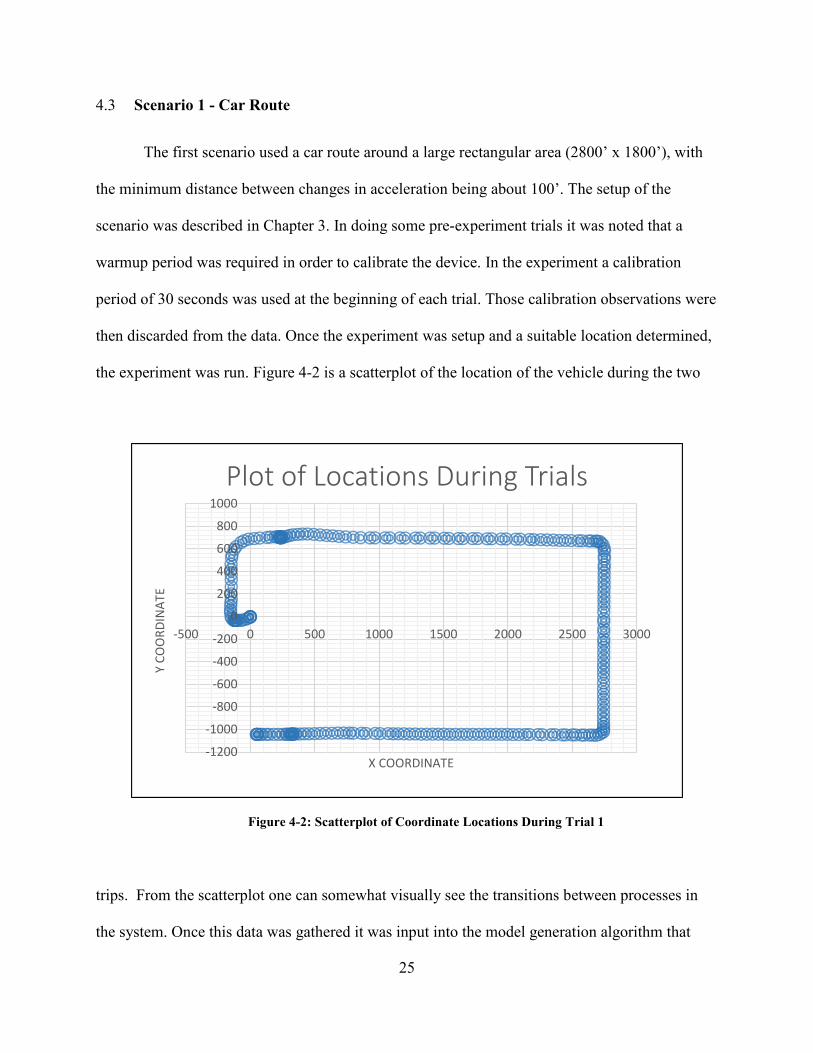
The first scenario used a car route around a large rectangular area (2800’ x 1800’), with
the minimum distance between changes in acceleration being about 100’. The setup of the
scenario was described in Chapter 3. In doing some pre-experiment trials it was noted that a
warmup period was required in order to calibrate the device. In the experiment a calibration
period of 30 seconds was used at the beginning of each trial. Those calibration observations were
then discarded from the data. Once the experiment was setup and a suitable location determined,
the experiment was run. Figure 4-2 is a scatterplot of the location of the vehicle during the two
trips. From the scatterplot one can somewhat visually see the transitions between processes in
the system. Once this data was gathered it was input into the model generation algorithm that
Figure 4-2: Scatterplot of Coordinate Locations During Trial 1
-1200
-1000
-800
-600
-400
-200
0
200
400
600
800
1000
-500 0 500 1000 1500 2000 2500 3000
Y CO
ORD
INAT
E
X COORDINATE
Plot of Locations During Trials
25

was previously developed. The accuracy of the model generated in this scenario is explored
further in section 4.3.2. This experiment seemed to suggest that when used on a large scale the
accuracy of the GPS was not an inhibiting factor in the accuracy of the programmatically
generated model. This suggests that the GPS tool would be, at least partially, capable of being
used in conjunction with the model generation algorithm to create models with movements that
occur on a large scale like simulations of transportation, supply-chain, logistics, etc.
4.3.1 Scenario 2 - Walking Route
The first scenario was successful in determining that in a situation where the scale of
movement was fairly large the accuracy of the GPS tool was not a significant factor. The purpose
of the second scenario was to determine the effect that variation in the tool had on the
algorithm’s model output when the movements between processes were smaller. This scenario
was done in an area that was about 20’X20’, and the minimum distance between steps was about
10’. The smaller distance between changes in velocity made it so that any inaccuracy of the GPS
tool would be more pronounced in the data that was collected. The accuracy of the
programmatically generated models is explored further in section 4.3.3.
4.3.2 Limitations of Data Gathering Tool
It was observed that the accuracy of the GPS data gathering tool could play a significant
role in the accuracy of the programmatically generated model. As seen in scenario 2, the
variation observed in the programmatically generated model was more than the variation that
was inherent in the process itself.
26

GPS accuracy is a factor of the device itself, as some GPS devices are more accurate than
others. The GPS device used in this research was not the market leader in accuracy, so it would
be feasible that greater accuracy could be achieved through a more precise and accurate GPS
system. The necessary amount of precision would be dependent on the physical scale of the
subject system, and the desired accuracy of the generated model. For instance, a system could be
in a small physical area where the GPS inaccuracy causes 10% more variation than would be
expected in the system. If in such a system the desired result was to determine if a simple change
would change the output of the system and the change caused a 100% increase in output, then it
may be reasonable to accept the inaccuracy of the GPS for the sake of further analysis. However,
that would have to be determined based on the risk tolerance of the person or organization that is
creating the simulation.
In order to determine the amount of variation that is being caused by the device it would
be necessary to do the following things:
1. Create a sample system where movements were on the same physical scale that
would be used in the subject system.
2. Apply sample speeds or delay times to each process in the sample system. This
can be done by sampling from a distribution or using a flat time.
3. Move the GPS device through the sample system.
4. Analyze the gathered data using the data analyzer.
27

5. Determine the variation caused by the inaccuracy of the GPS tool in the
programmatically generated model by comparing the processing times in the
sample system to the processing times in the programmatically generated
model.
6. Considering desired outcomes of the simulation model, determine if the tool
accuracy is unbearably high for the subject models physical scale.
Using this method it seems possible to determine if a specific GPS tool is accurate and precise
enough to be used in the method proposed in this research. If the above method suggests that it is
not suitable, then one could look into more accurate and precise GPS devices. If no GPS device
seems to work, then it would be necessary to gather coordinate locations in some other way. This
could feasibly be done using RFID mapping or by using a barcode scanner as a product enters
and exits a station and associating that station with a coordinate location. Each of these
techniques could be used with the same data analysis and model generation techniques to
programmatically generate a model. The difficulty with the alternative data gathering methods is
that they would require additional steps or resources that would not be necessary if one would be
able to use the simpler GPS data gathering method.
4.4 Programmatically Generated Model Accuracy
One of the important findings from this research is the accuracy that might be achieved in
various settings using the proposed data analysis algorithm. Each of the three subsequent
scenarios attempted to identify the possibilities and limitations of the proposed algorithm.
28

4.4.1 Generated Simulation
To create the data analysis algorithm a model was created in FlexSim, a simulation
software package. The model looked like what is seen in Figure 4-3 and had characteristics as
described in . A function was then written to get location data for 100 products as they moved
through the simulation. This data was then fed into the data analysis algorithm. The output of the
data analysis algorithm was then fed back into FlexSim by using the “FlexSim Data Translator”
code in Appendix C. The characteristics of this programmatically generated model were then
compared against the characteristics of the initial model, and a percent error was calculated.
Then both the models were run for 100 replications of 4000 time units, and some critical
statistics were compared. The comparison of characteristics and comparison of critical statistics,
Table 4-3: Error of Characteristics of Programmatically Generated Model
Table 4-4: Characteristics of Manually Generated Original Model
Object Characteristics Inputs Outputs Processing Time CapacitySource Processor 1Processor 1 Source Processor 2 triangular(15, 25.0, 20.0, 0) 1Processor 2 Processor 1,Processor 6 Processor 3 bernoulli(50, 10, 11, 0) 3Processor 3 Processor 2 Processor 4, Processor 5 exponential(10, 3, 0) 4Processor 4 Processor 3 Processor 6, Sink2 25 2Processor 5 Processor 3 Sink 1 20 1Processor 6 Processor 4 Processor 2 8 1Sink Processor 4, Processor 5
29

with their resultant percent error, can be found in Table 4-3. The visual comparison of the
simulation models can be seen in Figure 4-3. This data suggested an average 21% error in
estimating capacity, 9.92% error in estimating time within a step, and 7% accuracy in estimating
the throughput of a step. The error could be reduced even further in estimating the time within a
step if the distributions had been generated after checking for outliers. This would have resulted
in less than 1% error. The algorithm also created the exact flow from step to step within the
simulation.
Figure 4-3: Original (Top) and Programmatically Generated (Bottom) Simulations
30

These results were encouraging, because it meant that the algorithm was able to create a
fairly accurate representation of an original system using just the location data of the items as
they moved through the system. The minimal size of the error was especially impressive
considering the use of an overly simplistic distribution (see Appendix D).
4.4.2 Scenario 1 - Car Route
The setup of this scenario is described earlier, but the results showed that, when the
variation of the GPS is minimal when compared to the scope of the movement, it is possible to
create a fairly accurate simulation model to represent the system. When performing this
experiment the time in each segment of the car route was recorded. These times were then used
to create a simulation model using traditional model-building techniques and a simulation model
using the proposed methodology. The average times recorded for each segment of the drive
where then compared against the averages for each time segment from the manually and
programmatically generated simulation models (see Table 4-5 and
Table 4-6). The time to create the programmatically generated simulation model was also
compared against the time to create the manually generated simulation model. The model
building time for the programmatically generated simulation model was about 5 seconds. The
model building time for the manually generated simulation model was about 20 minutes. The
model building in both cases was done by someone experienced with the simulation software.
However, in the case of the programmatically generated model this experience was not
necessary, because the user had to merely run the function, and then select the output file created
by the data analysis algorithm. In this situation the time to create the programmatically generated
simulation model was just .4% of the time necessary to create the manually generated simulation
31
model, or 240X faster. However, it is likely that the relationship between programmatic and
manual model building time is not linear, because the program will take around 5 seconds
regardless of the scope of the model, and manual building time is highly dependent on the scope
of the model.
Table 4-5: Comparison of Observed and Generated Simulation Processing Times
Table 4-6: Comparison of Observed and Manual Simulation Processing Times
From this experiment it is evident that the algorithm was capable of generating a fairly
accurate simulation model when paired with the data collection system. There was significant
error (2.1-7.6%) between the generated model and the real-world system, and it is more than the
error that existed in the manually generated simulation model (.3-4.4%). However, it is feasible
to think of situations where the higher error could be traded off for the much faster model-
building capabilities of the algorithm.
Observed Average Simulation Average % ErrorProcess Input Output Trial 1 Trial 2 Trial 3 Trial 1 Trial 2 Trial 3 Trial 4 Trial 5Process 1 2 37.0 37.0 43.0 39.0 37.0 37.0 37.0 37.0 37.0 37.0 5.1%Process 2 1 3 58.0 29.0 52.0 46.3 48.5 55.0 42.6 45.0 23.0 42.8 7.6%Process 3 2 4 33.0 35.0 32.0 33.3 31.2 28.1 40.0 30.1 28.2 31.5 5.4%Process 4 3 5 43.0 45.0 42.0 43.3 40.3 41.3 40.5 40.1 40.6 40.5 6.4%Process 5 4 6 59.0 60.0 58.0 59.0 68.3 60.9 62.8 67.7 57.1 63.4 7.4%Process 6 5 22.0 24.0 22.0 22.7 22.6 22.1 24.9 22.3 24.8 23.3 3.0%Total 252.0 230.0 249.0 243.7 247.9 244.4 247.7 242.2 210.8 238.6 2.1%
Observed Generated Simulation
Observed Average Simulation Average % ErrorProcess Input Output Trial 1 Trial 2 Trial 3 Trial 1 Trial 2 Trial 3 Trial 4 Trial 5Process 1 2 37.0 37.0 43.0 39.0 40.9 40.6 38.0 39.7 41.2 40.1 2.8%Process 2 1 3 58.0 29.0 52.0 46.3 45.9 32.3 57.7 40.1 45.4 44.3 4.4%Process 3 2 4 33.0 35.0 32.0 33.3 32.4 32.7 32.4 33.3 32.5 32.6 2.1%Process 4 3 5 43.0 45.0 42.0 43.3 45.3 43.9 42.3 44.1 42.3 43.6 0.6%Process 5 4 6 59.0 60.0 58.0 59.0 60.1 59.3 60.0 58.3 59.2 59.4 0.6%Process 6 5 22.0 24.0 22.0 22.7 21.5 23.0 22.6 23.3 22.7 22.6 0.3%Total 252.0 230.0 249.0 243.7 246.2 231.7 253.0 238.7 243.3 242.6 0.5%
Observed Manual Simulation
32

4.4.3 Scenario 2 - Walking Route
The last scenario’s purpose was to test the robustness of the generated algorithm on a
small scale, where the system was near the edge of the accuracy of the GPS tool. In this scenario
the data was collected over five trials, using the flow and processing times characterized in Table
Process Input Output Processing Time CapacitySource Process 1
Process 1 Source Process 2 60 1Process 2 Process 1 Process 3 normal(120,30) 1Process 3 Process 2 Process 4, Process 5 normal(90,30) 1Process 4 Process 3 Process 5 75 1Process 5 Process 3, Process 4 Sink 120 1
Sink Process 5
Table 4-7: Characteristics of Walking Route System.
-30
-25
-20
-15
-10
-5
0
5
10
15
20
-40 -20 0 20 40 60 80 100
Position of Data Points
Trial 1 Trial 2 Trial 3 Trial 4 Trial 5
Figure 4-4: Position of Data Points in Scenario 2 Trials
33

4-7. When this data was then input in the data analysis algorithm, the algorithm was unable to
create a model that resembled the original system. This was largely due to the inability of the
GPS tool to be accurate to the precision necessary in the system. When the locations of each trial
were plotted, it was apparent that the tool was not capable of the precision necessary in this
system (see Figure 4-4). Therefore, at this level of detail it was not possible to create a model
that completely reflected the original system.
This scenario’s experiment shows that the data-gathering tool that was used had limited
ability to create useful data on this size system. These limitations could be analyzed and
overcome as described in section 4.2.3.
4.5 Capability of Proposed Model-Building Methodology
The proposed model-building methodology is capable of creating simulation models that
are fairly accurate in representing their real-world scenarios. However, the accuracy of the
simulation models is highly dependent on the comparative accuracy of the GPS data collection
tool in relation to the size of the subject system. As such, this methodology will likely become
more effective as the accuracy of such tools increases.
The results show that this methodology can produce simulations with error on system
throughput time at about 2% and error on an individual process time between 3% and 8% (see
Section 4.3.2). However, this methodology is not particularly good at estimating the true
capacity of individual processes in a system, as it was only capable of determining capacity with
a higher average error of 21% (see Section 4.3.1). This is the result of only being able to
determine capacity based off of observed limits in the context of the system instead of a
processes limit in isolation. The accuracy of other statistics was not analyzed as part of the
34

research. Therefore, the accuracy of additional statistics from a given model would have to be
tested against real-world observations to determine if the model was representative.
4.6 Time-Savings of Proposed Model-Building Methodology
The proposed model-building methodology seems to be successful in reducing the time
and software knowledge necessary to create a working model of a system. It does seem possible
to programmatically accomplish many of the model-building steps. From the car route scenario
(see Section 4.3.2) it was observed that the time to build a complete model manually with an
experienced modeler was about 240X longer than the time it took to build that model using the
proposed programmatic model-building methodology. It was also observed that the time
difference would increase non-linearly as each additional process would take much more time to
manually add to a simulation than each additional process would take to add programmatically.
A significant amount of the time difference is caused by the automated fitting of data using the
“Five-Point Distribution” (see Appendix D) instead of manually fitting each set of data to a
distribution. However, time savings were accomplished in each part of the model-building
process.
35
5 CONCLUSIONS
5.1 Limitations of Algorithm
The models generated using the proposed algorithm have many limitations. These
limitations are caused by the nature of the technique and by simplifying assumptions made
within the proposed algorithm.
The limitations caused by the simplifying assumptions of the proposed algorithm are not
a reflection of the method, but rather are a reflection of the limited scope of this research.
Therefore, these particular limitations could be overcome through further research. The
limitations caused by simplifying assumptions of the proposed algorithm include the following:
- Limited to a single type of product or item moving through the system
- Limited to probabilistic flow
- Identifying the differences between queues and processors
The limitations caused by the proposed methodology would be more difficult to
overcome with the current method, because the proposed method has no identifiable means of
overcoming these limitations. The limitations caused by the technique itself include the
following:
- Ignoring resources in the system
- Differentiating setup times within a process
- Inability to produce models for immobile systems 36

5.1.1 Algorithmic Limitations
Algorithmic limitations are limitations that are self-imposed on the presented research in
order to create a reasonable scope, and could be overcome in a fairly straightforward way with
additional research.
Single Product Type
The proposed algorithm was limited to being able to handle systems with a single type of
product or item. This limitation is merely a simplifying assumption of the research, as the
method could be expanded to systems that handle many different types of products. In order to
do that, the products would not only need a unique identifier attached to them as they move
through the system, but would also require a product type identifier that was unique to each
product type. Each product type could then be analyzed separately to determine flow. Pseudo-
capacity could be determined by finding a maximum number of each product that is ever in a
process at a time, and the maximum number of the combined products that is ever in the process
at a time. This could then be used to calculate a pseudo-capacity of the process given any product
mix. Further research could identify ways to more effectively handle systems with multiple
product types.
Probabilistic Flow
The proposed algorithm is limited to dealing with systems where flow is determined in a
probabilistic manner, or at least can be accurately represented in a probabilistic manner. A
system with this type of flow would send all the output of one process to the subsequent
processes using a fairly consistent percentage to each subsequent process. This is a significant
limitation, because it is common for a system to include at least one instance where flow can’t be
accurately depicted using probabilistic flow. A few common exceptions to this type of flow are
37
systems where flow is determined by sending the product to the first available subsequent
process, sending the product to subsequent processes in a round-robin manner, or sending the
product to a queue with the shortest waiting time. Each of these types of system flow could be
accurately identified in the proposed method, but the proposed algorithm only attempts to
identify the method for characterizing probabilistic flow. Each alternative flow method would
not be too difficult to implement in the algorithm, because once identified most simulation
software packages have built-in methods for building models with different flow characteristics.
Therefore, it would be necessary to identify the type of flow, include this information in the
algorithm output, and then adjust the software translator in order to include the information in the
programmatically generated model.
The first available flow method could be identified using a similar data gathering and
analysis method as presented in this research. Flow could be identified as “first-available” by
determining if the products used that method in the system. This would be done by looking to see
if the product predictably moved to the first available subsequent process. Availability of
subsequent processes would have to be determined by their pseudo-capacity, which may not be
completely accurate. However, a confidence level could be determined to estimate the flow type
as “first-available” if most of the time it did seem to use that method. The outlier instances could
then be used in a feedback loop to accurately adjust the pseudo-capacities.
The round-robin type of flow could be determined in a similar method. It could be
determined if the products moved from the process to the subsequent process by going to the
next possible subsequent process each time a product left the process. This could be combined
with the method for identifying the first-available type of flow in order to create first-available
round-robin flow, which is a common type of flow in many systems.
38

Other system flow types could be identified, and methods could be developed to identify
flow types and include them in the data analysis and model generation algorithm. Each of the
mentioned system flow characteristics could be included in the algorithm, but were not in order
to limit the scope of this particular research.
Processing Time vs. Delay Time Identification
One limitation inherent in the data collection method is an inability to instinctually
identify the difference between the time a product spends in the system being processed, and the
time a product spends in the system waiting or being delayed. This inability is caused by the
product constantly sending only movement location data while it is being tracked regardless of
whether it is simply waiting for availability. This limitation is slightly overcome in the proposed
algorithm by assuming that certain statistical representations of processes are more likely for
queues than processing steps, and in such a case the object should be modeled as a queueing step
in the system. This could also be overcome by identifying the subsequent steps after a process,
the flow of the system, and determining if the product is not moving to the subsequent step
because of a limit of the pseudo-capacity. If so, then the process would be modeled as a queue in
the system. If not, then the process would be modeled as a processing step in the system.
5.1.2 Methodical Limitations
Methodical limitations are those that are imposed by the proposed methodology. Most of
the methodical limitations are caused by the data collection method.
Modeling of Resources
One important limitation of the proposed methodology is the inability to account for
additional resources that are often required in a system. For instance, often an operator is shared
39

between machines and acts as a constraint on the system. This methodology would not be able to
accurately create models programmatically for systems where the resources play a significant
role in constraining the operation of the system. This limitation could feasibly be overcome by
tracking the location of the resources in the system and allocating them according to their
location, but this is not within the scope of this research.
Differentiating Setup Time from Process Time
Another limitation inherent in the data collection method is the inability to differentiate
between setup time and process time in a system. Unless the product moves between the setup
time and process time, there is no way to distinguish the difference between the two. This
limitation would be difficult to overcome purely using a tracking system, but could be overcome
with a hybrid system. A hybrid system would use a different data gathering method, but employ
the same data analysis and model building techniques proposed in this research. One example of
a hybrid system would be using a bar code scanner to track when a product enters a process,
when it starts processing at that process, and when it leaves each process in the system. The
processes would then be given a coordinate location. Data would then be generated to show the
coordinate location of the product at intervals during its time in the system. This data could then
be fed into the data analysis tool, and would allow for the separation of the setup and processing
times in the programmatically generated simulation.
Immobile Systems
The most obvious limitation of the proposed methodology is that the product must
physically move through the system, and that the movement through the system must be
representative of the processes being performed on the product. This is not true for every system.
Many systems have the product stationary and the work is done by resources moving to the
product. Some systems are hybrids where a part moves into a station where various tasks are 40

performed, and then it moves to the next station where various tasks are performed. In such a
hybrid situation it would be possible to create an initial model using this method, and then build
it out with the station details manually. The proposed data analysis method could also be adapted
to analyze data on events and tagged locations of a product in a system instead of physical
location, but that is not within the scope of this research.
5.2 Summary
The proposed model generating methodology consists of the data gathering tool, data
analysis algorithm, and simulation software data translator.
The data gathering tool is a GPS device that is attached to a product as it moves through a
system, and has a web browser that can access a PHP page with the code in Appendix A. The
data gathered in the tracking tool includes a unique identifier of the product being tracked, a GPS
latitude and longitude of the current position of the device, a unique identifier that distinguishes
product type, and the number of seconds that have elapsed since tracking began. This data is
captured at a consistent interval until the product has left the subject system.
The data gathered from the data gathering tool is used as input for the data analysis
algorithm. The data analysis algorithm assumes that changes in velocity of the object are
correlated with transitions between different steps in the system. Basically, the data gathering
tool attempts to convert the flow of the product through the system into discrete events that the
product experiences. This is accomplished by identifying processes that start and end when a
product experiences a period of acceleration above a defined threshold. The output of the data
analysis algorithm defines the location, flow, processing, and pseudo-capacity for a collection of
system processes.
41

The output of the data analysis algorithm is then translated by the simulation software
data translator. In this research a data translator was written for FlexSim simulation software.
The data translator takes the data analysis algorithm output and uses it to create a simulation.
By following these steps it is possible to create a simulation from product tracking data.
The accuracy of the model is not necessarily as good as it would be if the model was created
manually. However, for large simulation models the model-building time using this methodology
is significantly lower, because the model is programmatically built. Therefore, in order to
determine if this methodology would be practical a user of simulation software would have to
weigh the cost of time against the cost or inaccuracy. A user could also use the aforementioned
model building methodology to quicken the model building time by using the algorithm to create
a model with the basic logic, and then edit the model to add any custom logic. By doing this the
user could use the advantageous elements of the algorithm, but not be limited by as many of the
limitations.
There are many limitations to this model building methodology, as discussed in section
5.3. However, even with these limitations there seems to be a place for this methodology within
the set of useful simulation model building methodologies.
42

REFERENCES
Dangelmaier, W. and B. Mueck. “Using dynamic multiresolution modelling to analyze large material flow systems.” Proceedings of the 2004 Winter Simulation Conference, no. 2 (2004): 1720-1727.
Daniellmb. “Geolocation API on the iPhone.” (2009). http://stackoverflow.com/questions/221592/geolocation-api-on-the-iphone
Department of Defense. “Global Positioning System Standard Positioning Service Performance Standard, 4th Edition.” United States Department of Defense (2008).
Huber, D., M. Eberling, C. Laroque, and W. Dangelmaier. “Stochastic generation of discrete-event simulation models.” Inst. of Elec. and Elec. Eng. Computer Society (2008).
NGS. “Continuously Operating Reference Station (CORS).” National Geodetic Survey (2014). http://www.ngs.noaa.gov/CORS/
Pan, C., J. Lu, D. Wang, and B. Ran. “Data Collection Based on Global Positioning System for Travel Time and Delay for Arterial Roadway Network.” Transportation Research Record: Journal of the Transportation Research Board, no. 2024 (2007): 35-43.
Pradhananga, N. and J. Teizer. “Automatic spatio-temporal analysis of construction site equipment operations using GPS data.” Automation in Construction, v 29 (2013): 107-122.
Skoogh, A., B. Johansson, and J. Stahre. “Automated input data management: Evaluation of a concept for reduced time consumption in discrete event simulation” SIMULATION, no. 11 (2012): 1279-1293.
Spissu, E., I. Meloni, and B. Sanjust. “Behavioral Analysis of Choice of Daily Route with Data from Global Positioning System.” Transportation Research Record: Journal of the Transportation Research Board, no. 2230 (2011): 96-103.
United States Air Force. “Global Positioning System (GPS) IIF Satellite” (2014). http://www.losangeles.af.mil/library/factsheets/factsheet.asp?id=18670
43

APPENDICES
44
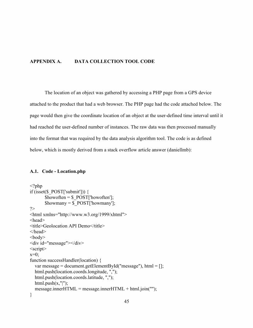
APPENDIX A. DATA COLLECTION TOOL CODE
The location of an object was gathered by accessing a PHP page from a GPS device
attached to the product that had a web browser. The PHP page had the code attached below. The
page would then give the coordinate location of an object at the user-defined time interval until it
had reached the user-defined number of instances. The raw data was then processed manually
into the format that was required by the data analysis algorithm tool. The code is as defined
below, which is mostly derived from a stack overflow article answer (daniellmb):
A.1. Code - Location.php
<?php if (isset($_POST['submit'])) { $howoften = $_POST['howoften']; $howmany = $_POST['howmany']; ?> <html xmlns="http://www.w3.org/1999/xhtml"> <head> <title>Geolocation API Demo</title> </head> <body> <div id="message"></div> <script> x=0; function successHandler(location) { var message = document.getElementById("message"), html = []; html.push(location.coords.longitude, ","); html.push(location.coords.latitude, ","); html.push(x,"|"); message.innerHTML = message.innerHTML + html.join(""); }
45

function errorHandler(error) {} function myTimer() { x=x+1 if (x==<?php echo $howmany; ?>) { clearInterval(myVar); } navigator.geolocation.getCurrentPosition(successHandler, errorHandler); } var myVar = setInterval(function(){myTimer()},<?php echo $howoften; ?>); </script> </body> </html> <?php } else { ?> <form action="" method="post"> How Many: <input type="text" name="howmany"><br> How Often: <input type="text" name="howoften"><br> <input type="submit" name="submit" value="Submit"> </form> <?php } ?>
46
APPENDIX B. DATA ANALYSIS ALGORITHM TOOL CODE
The “Data Analysis Algorithm Tool Code” was written in Excel VBA syntax. It contains
a module and a form. Also included is the code for a PHP page that the module uses to create
distributions for the processing steps.
B.1. Code - DataAnalysis Module
Public test_distance As Double Public test_time As Double Public test_acceleration As Double Public increment_time As Double Public fNameAcceleration As String Public fNameTime As String Dim last_location(2) As Double Dim x As Double Dim y As Double Dim z As Double Dim currentTime As Double Dim rowCount As Double Dim itemRow As Integer Dim temp_double As Double Dim temp_boolean As Boolean Dim itemNumber As Integer Dim startX As Double Dim startY As Double Dim inProcessor As Integer Dim processorNumber As Double Dim numberOfProcessors As Integer Dim processorDistanceStart As Double
47

Dim processorDistanceEnd As Double Dim dataArray() As Double Dim processorArray() As Double Dim timeArray() As Double Dim inProcessorArray() As Integer Dim processorInOut() As Double Dim flowLogic() As Integer Dim concatenateIn As String Sub DataAnalyzer() 'delete other worksheets Application.DisplayAlerts = False On Error Resume Next Sheets(3).Delete Sheets(2).Delete On Error GoTo 0 Application.DisplayAlerts = True 'start code rowCount = Range("A1000000").End(xlUp).Row test_distance = 1 test_time = 1 test_acceleration = 1 'x location last_location(0) = -100 'y location last_location(1) = -100 'type last_location(2) = -1 ' ' DataAnalyzer Macro ' Range("A1").Select Selection.SpecialCells(xlCellTypeConstants, 23).Select Selection.Copy Sheets.Add After:=ActiveSheet ActiveSheet.Paste Application.CutCopyMode = False ActiveWorkbook.Worksheets(2).Sort.SortFields.Clear ActiveWorkbook.Worksheets(2).Sort.SortFields.Add Key:=Range("D2:D" & rowCount) _ , SortOn:=xlSortOnValues, Order:=xlAscending, DataOption:=xlSortNormal ActiveWorkbook.Worksheets(2).Sort.SortFields.Add Key:=Range("A2:A" & rowCount) _ , SortOn:=xlSortOnValues, Order:=xlAscending, DataOption:=xlSortNormal
48

ActiveWorkbook.Worksheets(2).Sort.SortFields.Add Key:=Range("E2:E" & rowCount) _ , SortOn:=xlSortOnValues, Order:=xlAscending, DataOption:=xlSortNormal With ActiveWorkbook.Worksheets(2).Sort .SetRange Range("A1:E" & rowCount) .Header = xlYes .MatchCase = False .Orientation = xlTopToBottom .SortMethod = xlPinYin .Apply End With Sheets(2).Select Sheets(2).Name = "Analyzed Data" Range("F1").Select ActiveCell.FormulaR1C1 = "Distance" Range("G1").Select ActiveCell.FormulaR1C1 = "Velocity" Range("H1").Select ActiveCell.FormulaR1C1 = "Acceleration" Columns("F:H").Select Selection.ColumnWidth = 12.43 'fix some cells Range("f2:h2").Value = 0 'put in the distance,velocity, and acceleration Range("F3").Select ActiveCell.FormulaR1C1 = _ "=R[-1]C+SQRT(((RC[-4]-R[-1]C[-4])^2)+((RC[-3]-R[-1]C[-3])^2))" Range("F3").Select Selection.AutoFill Destination:=Range("F3:F" & rowCount) Range("F3:F" & rowCount).Select Range("G3").Select ActiveCell.FormulaR1C1 = "=RC[-1]-R[-1]C[-1]" Range("G3").Select Selection.AutoFill Destination:=Range("G3:G" & rowCount) Range("G3:G" & rowCount).Select Range("H3").Select ActiveCell.FormulaR1C1 = "=abs(RC[-1]-R[-1]C[-1])" Range("H3").Select Selection.AutoFill Destination:=Range("H3:H" & rowCount) 'set a default test acceleration by normalizing the data and then finding outliers Dim groupSize As Integer Dim groupMean(9) As Double Dim theRange As String groupSize = rowCount / 10 For x = 0 To 9
49
theRange = Range("h" & ((x * groupSize) + 2) & ":h" & (((x + 1) * groupSize) + 1)).Address groupMean(x) = Application.WorksheetFunction.Sum(Range(theRange)) / groupSize Next For x = 0 To 9 Range("I" & (x + 2)).Value = groupMean(x) Next increment_time = Range("e3").Value - Range("e2").Value test_acceleration = Application.WorksheetFunction.Quartile_Inc(Range("I2:I11"), 1) - (1.5 * (Application.WorksheetFunction.Quartile_Inc(Range("I2:I11"), 3) - Application.WorksheetFunction.Quartile_Inc(Range("I2:I11"), 1))) X_CreateAccelerationChart X_CreateTimeChart settings.Show End Sub Sub DataTests() 'do all the tests according to the sensitivities For x = 2 To rowCount temp_boolean = False 'do the acceleration test If IsNumeric(Range("H" & x).Value) Then temp_double = Range("H" & x).Value Else temp_boolean = True temp_double = 0 End If If temp_double > test_acceleration Or temp_boolean = True Then temp_boolean = True Else temp_boolean = False End If Range("I" & x).Value = temp_boolean 'do the time test temp_boolean = False For y = 1 To (test_time / increment_time) If ((x - y) < 1) Or (Range("D" & (x - y)).Value <> Range("D" & x).Value) Then Exit For If Range("I" & (x - y)).Value = True Then temp_boolean = True Next y If temp_boolean = True Then Range("J" & x).Value = False ElseIf Range("I" & x).Value = True Then Range("J" & x).Value = True Else Range("J" & x).Value = False End If
50
'do the distance test If (Range("d" & x).Value <> last_location(2)) Then Range("K" & x).Value = True last_location(2) = Range("d" & x).Value Else If (Range("I" & x).Value = True) And (Sqr(((Range("b" & x).Value - last_location(0)) ^ (2)) + ((Range("c" & x).Value - last_location(1)) ^ (2))) > test_distance) Then Range("K" & x).Value = True last_location(0) = Range("b" & x).Value last_location(1) = Range("c" & x).Value Else Range("K" & x).Value = False End If End If 'see when all the tests pass If (Range("I" & x).Value = True And Range("J" & x).Value = True And Range("K" & x).Value = True) Or Range("a" & x).Value <> Range("a" & (x - 1)).Value Then Range("L" & x).Value = True Else Range("L" & x).Value = False End If Next x ProcessorCreate End Sub Sub ProcessorCreate() 'create a sheet to store the runtimes Sheets.Add After:=ActiveSheet Sheets(3).Select Sheets(3).Name = "Processors" Cells(1, 1) = "Number" Cells(1, 2) = "Start X" Cells(1, 3) = "End X" Cells(1, 4) = "Start Y" Cells(1, 5) = "End Y" Cells(1, 6) = "Angle" Cells(1, 7) = "Length" Cells(1, 8) = "IN" Cells(1, 9) = "OUT" Cells(1, 10) = "Times" Sheets(2).Select 'redim dataArray to put data in it ReDim dataArray((rowCount - 1), 4) For x = 0 To (rowCount - 2) dataArray(x, 0) = Cells(x + 2, 1) dataArray(x, 1) = Cells(x + 2, 2)
51
dataArray(x, 2) = Cells(x + 2, 3) dataArray(x, 3) = Cells(x + 2, 5) dataArray(x, 4) = Cells(x + 2, 12) Next x 'processorNumber for processor # processorNumber = 0 currentTime = 0 startX = Range("b2").Value startY = Range("c2").Value For x = 0 To (rowCount - 2) If dataArray(x, 4) = True Then processorNumber = processorNumber + 1 Next x 'size the processor array ReDim processorArray(processorNumber, 6) ReDim timeArray(processorNumber, 1000) ReDim inProcessorArray(processorNumber, 1000) 'fill the arrays For x = 0 To processorNumber For y = 0 To 6 processorArray(x, y) = -100 Next y For y = 0 To 1000 timeArray(x, y) = -100 inProcessorArray(x, y) = -100 Next y Next x 'find the max time maxTime = 0 For x = 0 To (rowCount - 1) If (dataArray(x, 3) > maxTime) Then maxTime = dataArray(x, 3) Next x timeArraySize = maxTime * (1 / increment_time) Dim locationAtTime() As Double ReDim locationAtTime(timeArraySize, processorNumber) 'go through the data array numberOfProcessors = processorNumber processorNumber = 0 For x = 0 To (rowCount - 2) If dataArray(x, 0) <> itemNumber Then itemNumber = dataArray(x, 0) startX = dataArray(x, 1) startY = dataArray(x, 2) currentTime = dataArray(x, 3) inProcessor = -1 ElseIf x = (rowCount - 2) Or dataArray((x + 1), 4) = True Then
52
For z = 0 To numberOfProcessors processorDistanceStart = Sqr(((processorArray(z, 1) - startX) ^ (2)) + ((processorArray(z, 3) - startY) ^ (2))) processorDistanceEnd = Sqr(((processorArray(z, 2) - dataArray(x, 1)) ^ (2)) + ((processorArray(z, 4) - dataArray(x, 2)) ^ (2))) If processorDistanceStart < test_distance And processorDistanceEnd < test_distance Then processorNumber = z startX = dataArray((x + 1), 1) startY = dataArray((x + 1), 2) 'need to record the inProcessor in another array For y = 0 To 1000 If inProcessorArray(processorNumber, y) = -100 Then Exit For Next y inProcessorArray(processorNumber, y) = inProcessor inProcessor = processorNumber 'record the times in another array For y = 0 To 1000 If timeArray(processorNumber, y) = -100 Then Exit For Next y timeArray(processorNumber, y) = dataArray(x, 3) - currentTime currentTime = dataArray(x, 3) Exit For ElseIf processorArray(z, 1) = -100 Then processorNumber = z processorArray(processorNumber, 0) = processorNumber processorArray(processorNumber, 1) = startX startX = dataArray((x + 1), 1) processorArray(processorNumber, 2) = dataArray(x, 1) processorArray(processorNumber, 3) = startY startY = dataArray((x + 1), 2) processorArray(processorNumber, 4) = dataArray(x, 2) 'need to record the inProcessor in another array For y = 0 To 1000 If inProcessorArray(processorNumber, y) = -100 Then Exit For Next y inProcessorArray(processorNumber, y) = inProcessor inProcessor = processorNumber 'record the times in another array For y = 0 To 1000 If timeArray(processorNumber, y) = -100 Then Exit For Next y timeArray(processorNumber, y) = dataArray(x, 3) - currentTime currentTime = dataArray(x, 3) Exit For End If
53

Next z Else 'add to the array with the items current timePos = dataArray(x, 3) * (1 / increment_time) locationAtTime(timePos, processorNumber) = locationAtTime(timePos, processorNumber) + 1 End If Next x 'print the processor array data to the sheet Sheets(3).Select For x = 0 To numberOfProcessors For y = 0 To 5 If processorArray(x, y) <> -100 Then Cells(x + 2, y + 1).Value = processorArray(x, y) Next y Next x 'calculate the angles and lengths y = Range("A1000000").End(xlUp).Row For x = 2 To y Range("f" & x).Formula = "=IF(B" & x & ">C" & x & ",DEGREES(ATAN((E" & x & "-D" & x & ")/(C" & x & "-B" & x & ")))+180,DEGREES(ATAN((E" & x & "-D" & x & ")/(C" & x & "-B" & x & "))))" Next x For x = 2 To y Range("g" & x).Formula = "=SQRT(((C" & x & "-B" & x & ")^2)+((E" & x & "-D" & x & ")^2))" Next x 'print the inProcessorArray ' y=lastrow z = y ReDim processorInOut((y - 2), 1) ReDim flowLogic((y - 2), (y - 2)) 'change this so that it compares the number of processors out For x = 0 To z - 2 For y = 0 To 1000 'concatenate them all 'And InStr(concatenateIn, timeArray(x, y)) = False If timeArray(x, y) <> -100 Then If inProcessorArray(x, y) <> -1 Then processorInOut(x, 0) = processorInOut(x, 0) + 1 processorInOut(inProcessorArray(x, y), 1) = processorInOut(inProcessorArray(x, y), 1) + 1 'increment an array of size (# of processors)X(# of processors), so that we can determine later how many went where flowLogic(inProcessorArray(x, y), x) = flowLogic(inProcessorArray(x, y), x) + 1 End If End If
54

Next y Next x 'find sources and sinks For x = 0 To z - 2 If (processorInOut(x, 0) - processorInOut(x, 1)) > 0 Then Range("i" & (x + 2)).Value = "test|-2`" & Round(((processorInOut(x, 0) - processorInOut(x, 1)) / processorInOut(x, 0)), 4) End If Next x 'put in a unique list For x = 0 To (z - 2) For y = 0 To 1000 If timeArray(x, y) <> -100 And InStr(concatenateIn, "~" & inProcessorArray(x, y)) = False Then If (inProcessorArray(x, y) >= 0) Then If (processorInOut(inProcessorArray(x, y), 1) = 0) Then percentFlow = 1 Else percentFlow = Round((flowLogic(inProcessorArray(x, y), x) / processorInOut(inProcessorArray(x, y), 1)), 4) End If concatenateIn = concatenateIn & "~" & inProcessorArray(x, y) & "`" & percentFlow Else concatenateIn = concatenateIn & "~" & inProcessorArray(x, y) & "`" & 1 End If End If Next y concatenateIn = Mid(concatenateIn, 2) Cells(x + 2, 8) = "test|" & concatenateIn concatenateIn = "" Next x 'print the time array data to the sheet For x = 0 To (z - 2) For y = 0 To 1000 If timeArray(x, y) <> -100 Then If timeArray(x, y) <> -1 Then concatenateIn = concatenateIn & "~" & timeArray(x, y) Else concatenateIn = concatenateIn & "~" & "Source" End If End If Next y concatenateIn = Mid(concatenateIn, 2) Cells(x + 2, 10) = concatenateIn concatenateIn = "" Next x
55

'find the pseudo-capacity of each processor Dim processorCapacity() As Integer ReDim processorCapacity(z - 2) For t = 0 To UBound(locationAtTime, 1) For x = 0 To (z - 2) If (locationAtTime(t, x) > processorCapacity(x)) Then processorCapacity(x) = locationAtTime(t, x) Next x Next t 'put the pseudo-capacity in column L and label the column For x = 0 To (z - 2) Cells(x + 2, 12) = processorCapacity(x) Next x Cells(1, 12) = "Pseudo-Capacity" 'Get the number of processors that we have y = Cells(Rows.Count, "A").End(xlUp).Row - 2 'Go through each processor and create a web query to ge the distribution For x = 0 To y Range("K" & (x + 2)).Select With ActiveSheet.QueryTables.Add(Connection:= _ "URL;http://www.descreye.com/distribution-fitting.php?processing_times=" & Range("J" & (x + 2)).Value _ , Destination:=Range("$K$" & (x + 2))) '.CommandType = 0 .Name = Range("J" & (x + 2)).Value .FieldNames = True .RowNumbers = False .FillAdjacentFormulas = False .PreserveFormatting = True .RefreshOnFileOpen = False .BackgroundQuery = True .RefreshStyle = xlInsertDeleteCells .SavePassword = False .SaveData = True .AdjustColumnWidth = True .RefreshPeriod = 0 .WebSelectionType = xlAllTables .WebFormatting = xlWebFormattingNone .WebPreFormattedTextToColumns = True .WebConsecutiveDelimitersAsOne = True .WebSingleBlockTextImport = False .WebDisableDateRecognition = False .WebDisableRedirections = False .Refresh BackgroundQuery:=False End With Next x
56

SaveSheetCSV End Sub Sub X_CreateAccelerationChart() Dim accelerationChart As Object 'get the number of rows of the first item Sheets(2).Select For x = 2 To rowCount If (Range("a" & x).Value <> Range("a" & (x + 1)).Value) Then Exit For Next Range("H1:H" & x).Select ActiveSheet.Shapes.AddChart2(227, xlLine).Select ActiveChart.SetSourceData Source:=Range("'Analyzed Data'!$H$1:$H$" & x) Range("I2").Select ActiveCell.FormulaR1C1 = test_acceleration Selection.AutoFill Destination:=Range("I2:I" & x), Type:=xlFillDefault Range("I2:I21").Select ActiveSheet.ChartObjects(1).Activate Set accelerationChart = ActiveSheet.ChartObjects(1).Chart accelerationChart.SeriesCollection.NewSeries accelerationChart.FullSeriesCollection(2).Values = "='Analyzed Data'!$I$2:$I$" & x accelerationChart.FullSeriesCollection(2).XValues = "='Analyzed Data'!$E$2:$E$" & x accelerationChart.SetElement (msoElementChartTitleAboveChart) accelerationChart.ChartTitle.Text = "Acceleration" fNameAcceleration = ThisWorkbook.Path & "\acceleration.gif" accelerationChart.Export fileName:=fNameAcceleration, FilterName:="GIF" ActiveSheet.ChartObjects(1).Delete End Sub Sub X_CreateTimeChart() Dim timeChart As Object Dim lastRow As Integer Dim lastTime As Double lastTime = 0 y = 2 'create the data for the chart 'clear j column Range("j:j").Value = "" 'get the number of rows of the first item Sheets(2).Select For x = 3 To rowCount If (Range("a" & x).Value <> Range("a" & (x + 1)).Value) Then Exit For If (Range("h" & x).Value > Range("i" & x).Value) Then Range("j" & y).Value = Range("e" & x).Value - lastTime lastTime = Range("e" & x).Value y = y + 1
57

End If Next x 'get the last row lastRow = Range("J1000000").End(xlUp).Row 'set the current line Range("K2:K" & (y - 1)).Value = test_time 'make the scatterplot Range("J2:J" & lastRow).Select ActiveSheet.Shapes.AddChart2(240, xlXYScatter).Select ActiveChart.SetSourceData Source:=Range("'Analyzed Data'!$J$2:$J$" & lastRow) ActiveChart.SeriesCollection.NewSeries ActiveChart.FullSeriesCollection(2).Values = "='Analyzed Data'!$K$2:$K$" & (y - 1) ActiveChart.ChartTitle.Text = "Time Values" fNameTime = ThisWorkbook.Path & "\time.gif" ActiveChart.Export fileName:=fNameTime, FilterName:="GIF" ActiveSheet.ChartObjects(1).Delete End Sub Sub SaveSheetCSV() Dim fNameTable As String fNameTable = ThisWorkbook.Path & "\table.csv" Sheets(3).SaveAs fileName:=fNameTable, FileFormat:=xlCSV End Sub Sub DeleteCreatedSheets() Application.DisplayAlerts = False On Error Resume Next Sheets(3).Delete Sheets(2).Delete On Error GoTo 0 Application.DisplayAlerts = True End Sub
B.2. Code - Settings Form
Private Sub cmd_submit_Click() test_acceleration = settings.inp_acceleration.Value test_distance = settings.inp_distance.Value test_time = settings.inp_time.Value DataAnalysis.DataTests settings.Hide Kill (fNameAcceleration) Kill (fNameTime)
58

End Sub Private Sub inp_acceleration_Change() If IsNumeric(settings.inp_acceleration.Value) = True Then test_acceleration = settings.inp_acceleration.Value DataAnalysis.X_CreateAccelerationChart DataAnalysis.X_CreateTimeChart img_acceleration.Picture = LoadPicture(fNameAcceleration) img_time.Picture = LoadPicture(fNameTime) End If End Sub Private Sub inp_increment_Change() increment_time = settings.inp_increment.Value End Sub Private Sub inp_time_Change() If IsNumeric(settings.inp_time.Value) = True Then test_time = settings.inp_time.Value DataAnalysis.X_CreateTimeChart img_time.Picture = LoadPicture(fNameTime) End If End Sub Private Sub UserForm_Initialize() settings.inp_increment.Value = increment_time settings.inp_acceleration.Value = test_acceleration settings.inp_distance.Value = test_distance settings.inp_time.Value = test_time img_acceleration.Picture = LoadPicture(fNameAcceleration) img_time.Picture = LoadPicture(fNameTime) End Sub Private Sub UserForm_Terminate() Kill (fNameAcceleration) Kill (fNameTime) End Sub
B.3. Code - Distribution-Fitting.php
<?php
59

function get_quartile($Array, $Quartile) { $pos = (count($Array) - 1) * $Quartile; $base = floor($pos); $rest = $pos - $base; if( isset($Array[$base+1]) ) { $return_value = $Array[$base] + $rest * ($Array[$base+1] - $Array[$base]); } else { $return_value = $Array[$base]; } //echo $return_value."<br>"; return $return_value; } $times = $_REQUEST['processing_times']; $times = explode('~',$times); sort($times); $quartile = array(); $quartile['0']=get_quartile($times,0); $quartile['.2']=get_quartile($times,.2); $quartile['.4']=get_quartile($times,.4); $quartile['.6']=get_quartile($times,.6); $quartile['.8']=get_quartile($times,.8); $quartile['1']=get_quartile($times,1); $distribution_text = "fivepointdistribution("; foreach ($quartile as $value) $distribution_text.="~".$value; $distribution_text.=")"; $distribution_text = str_replace("(~","(",$distribution_text); echo "<table><tr><td>".$distribution_text."</td></tr></table>"; ?>
60

APPENDIX C. FLEXSIM DATA TRANSLATOR CODE
The “FlexSim Data Translator Code” allows FlexSim to translate the data output by the
“Data Analysis Algorithm Tool Code” into the simulation software package. It includes two
functions that make this possible. One is the function that creates the model, and that is called
modelimport. The other function, fivepointdistribution, allows the use of the previously
discussed and custom five-point distribution in FlexSim. The code for each function is written in
FlexSim’s own language, FlexScript.
C.1. Code - FlexSim Function: ModelImport
/**Custom Code*/ nodeinsertinto(model()); setname(last(model()), "ModelData"); treenode ModelData = node("/ModelData",model()); string fileName = filebrowse("*.csv","Model Data CSV",pdir()); importtable(ModelData,fileName,0,0); int numberOfProcessors = content(ModelData); //create the processors for (int x=2; x<=numberOfProcessors; x++) { createinstance(node("/fixedresources/Processor",library()),model()); treenode processor = last(model()); string processorName = concat("Processor",numtostring(getnodenum(rank(rank(ModelData,x),1)))); double processorLength = getnodenum(rank(rank(ModelData,x),7)); double processorAngle = getnodenum(rank(rank(ModelData,x),6)); double processorXLoc = getnodenum(rank(rank(ModelData,x),2)); double processorYLoc = getnodenum(rank(rank(ModelData,x),4));
61
string processorDistribution = concat("return ",getnodestr(rank(rank(ModelData,x),11)),";"); double processorMaxContent = getnodenum(rank(rank(ModelData,x),12)); processorDistribution = stringreplace(processorDistribution,"~",","); //adjust for bad positioning processorYLoc = ((processorLength*sin(degreestoradians(processorAngle)))/2)+processorYLoc; processorXLoc = processorXLoc-((processorLength/2)-((processorLength/2)*cos(degreestoradians(processorAngle)))); //set everything setname(processor, processorName); setsize(processor, processorLength,.1,.1); setrot(processor,0,0, processorAngle); setloc(processor,processorXLoc,processorYLoc,0); setnodestr(node(">variables/cycletime",processor),processorDistribution); setnodenum(node(">variables/maxcontent",processor),processorMaxContent); } //create the sinks for (int x=2; x<=numberOfProcessors; x++) { string flowString = getnodestr(rank(rank(ModelData,x),9)); //this data is a string with the port to connect followed by the percentage of the inputs flow that goes to the current object //cut the fluff part if (stringlen(flowString)>0){ flowString = stringcopy(flowString, 6,stringlen(flowString)-6); int sep = stringsearch(flowString,"`",0); string inputProcStr = stringcopy(flowString,1,sep); int inputProc = stringtonum(inputProcStr); double inputProb = stringtonum(stringcopy(flowString,sep+2,(stringlen(flowString)-sep)-1)); createinstance(node("/fixedresources/Sink",library()),model()); treenode newSink = last(model()); setname(newSink, concat("Sink",numtostring(x))); setloc(newSink, getnodenum(rank(rank(ModelData,x),3))+1, getnodenum(rank(rank(ModelData,x),5)),0); treenode inProcessor = rank(model(),x+2); contextdragconnection(inProcessor,newSink,"A"); //add a label to the inProcessor with the amount of it that goes to this sink addlabel(inProcessor,"Sink",inputProb); } } //create the connnections for (int x=2; x<=numberOfProcessors; x++) {
62

string flowString = getnodestr(rank(rank(ModelData,x),8)); //this data is a string with the port to connect followed by the percentage of the inputs flow that goes to the current object //cut the fluff part int flowStringLen = stringlen(flowString); flowString = stringcopy(flowString, 6,flowStringLen-5); //go through the string making each connection int found = 0; string currentString = ""; int sep = 0; string inputProcStr = ""; int inputProc = 0; double inputProb = 0; while (found>=0) { found = stringsearch(flowString,"~",0); if (found>0) { currentString = stringcopy(flowString,1,found); } else { currentString = flowString; found=-1; } //this is now just a incoming connection and a probability, seperate those sep = stringsearch(currentString,"`",0); inputProcStr = stringcopy(currentString,1,sep); inputProc = stringtonum(inputProcStr); inputProb = stringtonum(stringcopy(currentString,sep+2,(stringlen(currentString)-sep)-1)); //we should now have the input object and the probability to go to the current object from the input object //make the connection if (inputProc>=0) { //it is a processor treenode inProcessor = rank(model(),inputProc+4); treenode outProcessor = rank(model(),x+2); contextdragconnection(inProcessor,outProcessor,"A"); addlabel(inProcessor,concat("Flow",numtostring(x)),inputProb); } else { //it is a source createinstance(node("/fixedresources/Source",library()),model()); treenode newSource = last(model()); setname(newSource, concat("Source",numtostring(x)));
63
setloc(newSource, getnodenum(rank(rank(ModelData,x),2))-1, getnodenum(rank(rank(ModelData,x),4)),0); setvarstr(newSource,"interarrivaltime","return 0;"); //create connections treenode outProcessor = rank(model(),x+2); contextdragconnection(newSource,outProcessor,"A"); } //set the probability flow function //take off the current part of the flowString if (found>=0) flowString = stringcopy(flowString,found+2,(stringlen(flowString)-found-1)); } } //use the labels to create the flow probabilities string starter = "double randomnum = uniform(0.0, 100.0, 0);double total = 0.0;"; for (int x=2; x<=numberOfProcessors; x++) { treenode proc = rank(model(),x+2); double remaining = 1; string flowCode = starter; for (int y=1;y<=content(labels(proc));y++) { if (stringsearch(getnodename(label(proc,y)),"Sink",0)>=0) { double percentage = getlabelnum(proc,y)*100; flowCode = concat(flowCode,"total += ",numtostring(percentage),";if (randomnum <= total) return ",numtostring(y),";"); remaining = 1-(percentage/100); } else { double percentage = getlabelnum(proc,y)*100; flowCode = concat(flowCode,"total += ",numtostring(percentage*remaining),";if (randomnum <= total) return ",numtostring(y),";"); } } flowCode = concat(flowCode,"return 1;"); switch_flexscript(getvarnode(proc,"sendtoport"),1); setvarstr(proc,"sendtoport",flowCode); buildnodeflexscript(getvarnode(proc,"sendtoport")); }
64

C.2. Code - FlexSim Function: FivePointDistribution
/**Custom Code*/ int quartile_end = duniform(2,6); int quartile_beg = quartile_end-1; double ran domnumber = uniform(parval(quartile_beg),parval(quartile_end)); return randomnumber;
65

APPENDIX D. FIVE-POINT DISTRIBUTION
D.1. Explanation
The proposed “five-point distribution” is merely a collection of 5 uniform distributions
that are used to approximate a more advanced statistical distribution. In order to create the
distribution six percentiles in the data are found; 0, .2, .4, .6, .8, 1. For instance, assume the
following was an observed data set:
106, 110, 108, 100, 103, 101, 114, 102, 102, 103, 108, 100, 114, 105, 113, 104, 111, 104,
104, 100, 114, 100, 101, 114, 110, 102, 100, 109, 119, 100, 107, 122, 106, 103, 103, 102, 101,
102, 114, 114, 102, 110, 105, 100, 129, 107, 103, 111, 111, 113
The six percentiles calculated would be the following:
100, 101.8, 103, 107.4, 113, 129
The probability density curve of the resultant distribution looks like what is seen in the
figure on the following page.
66

To sample from this distribution two random numbers are then generated the first is a
random number sampled from a uniform distribution between 0 and 1. That random number is
then used to determine what range will be used for the second random number. In the example if
.22 was our first random number, then the second random number would be sampled from a
uniform distribution between 101.8 and 103. That number would then be the sample from the
distribution.
There are a few advantages and disadvantages to using this distribution. One advantage is
the all-encompassing nature of the distribution. This distribution adapts to the dataset, so it can
fit the distribution regardless of the skew or normality. This advantage also makes fitting data to
the distribution very simple. Six quick calculations provide all the information that is necessary
to create the distribution. One disadvantage of the distribution is that it is less precise than a
better fitted distribution. It also would have difficulty with any data that has more than two
modes, because using only five uniform distributions would not approximate a bimodal
0
0.02
0.04
0.06
0.08
0.1
0.12
0.14
0.16
0.18
97 99 101 103 105 107 109 111 113 115 117 119 121 123 125 127 129 131
Probability Density of Five-Point Distribution
Probability Density Function of the Example Five-Point Distribution.
67

distribution as effectively. This could be done by using more uniform (i.e. ten) distributions to
represent the bimodal data. This would be using the same concept but use ten points instead of
five.
68


![Defense-related Applications of Discrete Event Simulation · Defense-related Applications of Discrete Event Simulation. ... [Banks, 2010] Defense-related ... • Randomness in discrete](https://img.pdfslide.us/doc/110x75/5ae74c3d7f8b9a6d4f8dde4b/defense-related-applications-of-discrete-event-simulation-applications-of-discrete.jpg)