Embed Size (px)
Citation preview

The Productivity Effects of Stock Option Schemes: Evidence from Finnish Panel Data1
REVISED May 19, 2006 Derek C. Jones Dept. of Economics, Hamilton College, Clinton, NY 13323, [email protected] Panu Kalmi Dept. of Economics, Helsinki School of Economics and HECER, PO Box 1210, 00101 Helsinki, Finland, [email protected] Mikko MÄKINEN (corresponding author) The Research Institute of the Finnish Economy ETLA, Lönnrotinkatu 4 A, FIN-00120 Helsinki, Finland, [email protected] and Helsinki School of Economics Abstract: While theorists differ sharply on the expected economic impact of stock options, typically empirical work has found a positive association between option schemes and firm productivity. However, existing data are limited and may not enable reliable investigation of the productivity effects. New panel data for all Finnish publicly listed firms during 1992-2002 enable us to distinguish plans that are broad based and others limited to particular employees and address issues of endogeneity concerning inputs and options. Diverse specifications are estimated including dynamic panel data models with a GMM estimator. For broad-based option scheme indicators the key result is that different estimators consistently find statistically insignificant associations with firm productivity. For selective option schemes, the baseline fixed effects estimator suggests a 2.1-2.4% positive and statistically significant effect on firm productivity. However, in empirical models in which endogeneity and dynamics are taken into account, no evidence is found of a link with firm productivity. Thus our findings are consistent with hypotheses that predict negligible effects of option plans for enterprise performance, such as those based on free riding, or psychological expectancy theory or accounting myopia. However, by finding weak evidence for productivity effects of targeted schemes (and none for broad-based plans) our findings tend not to support hypotheses based on managerial rent seeking. Keywords: personnel economics, stock options, productivity, panel data JEL-codes: M5, J3, L2, C3

2
1. Introduction
During the 1990s, stock options became an increasingly popular compensation
method in many countries (e.g. Hall, 1998; Murphy, 1999). Initially, option programs
were typically allocated, almost without exception, only to executives.2 But this
association of stock options mainly with managerial compensation changed rapidly
after more and more companies worldwide started to issue stock options to the
workforce more broadly (e.g. Weeden, Carberry and Rodrick, 1998; Lebow, Sheiner,
Slifman and Starr-McCluer, 1998; and Blasi, Kruse and Bernstein, 2003). In turn this
growth of stock options has generated heated public discussion with some viewing
stock options as a device by which managers transfer excessive benefits to themselves,
while others see options as a major innovation in managerial and personnel
compensation.
The growth of options has also been accompanied by a mushrooming of
theoretical and empirical literature on stock options (e.g. Ittner, Lambert and Larcker,
2003). Whereas sharp disagreements exist among theorists on the expected economic
impact of different types of option schemes, existing empirical work consistently finds
that firm performance is enhanced by stock options. However, the findings based on
existing empirical work are potentially limited. Empirical analysis has been forced to
rely on data that may not be representative, typically are for only short time periods and
are mainly for the U.S. and the U.K. (e.g. Conyon and Freeman, 2004; Sesil,
Kroumova, Blasi and Kruse, 2002). Moreover, existing data may not enable a careful
investigation of the productivity effects of different types of option plans.
By contrast in this paper we use new panel data that we have assembled. The
data include all Finnish publicly listed firms during a relatively long period, namely
1992-2002. Thus it enables us to see if previous findings based mainly on evidence
generated using US and UK data, are applicable to another country which once had a

3
very different system of corporate governance but which has recently moved to adopt
an Anglo-Saxon model. In our empirical work we estimate Cobb-Douglas production
functions with different stock option program indicators. Furthermore, whereas earlier
empirical literature has used cross-section and fixed effects models, we also address the
potentially important issue of endogeneity of inputs and options by estimating dynamic
panel data models with a GMM estimator.
For broad-based option scheme indicators the key result is that different
estimators consistently find a statistically insignificant association with firm
productivity. For selective option schemes, the baseline fixed effects estimator suggests
a 2.1-2.4% positive and statistically significant effect of the dilution indicator on firm
productivity. However, in empirical models in which endogeneity and dynamics are
accounted for, no evidence is found of a link with firm productivity. Insofar as our
findings do not provide support for hypotheses of a positive association between option
schemes and firm productivity, our findings differ in important ways from earlier
findings that are based on less rigorous methods and more limited data.
This paper is organised as follows. Section 2 provides the conceptual
underpinnings for the study and also surveys relevant empirical research on the
productivity effects of stock options and related schemes. In section 3 we describe the
institutional framework and our most unusual data. Section 4 outlines our empirical
strategy and this is followed by a presentation of our findings. In the final section we
provide conclusions and implications of the paper.
2. Conceptual Framework and Previous Empirical Work
A key argument of proponents of stock options is that options can align the
interest of employees and shareholders. For example, stock options may motivate
employees to exert more effort and take actions that are mutually beneficial to both
4
owners and employees. The motivational effect of stock options may be especially
relevant in situations where alternative approaches, such as direct monitoring or piece
rates, are not feasible, perhaps because of monitoring difficulties (Sesil, Kroumova,
Blasi and Kruse, 2002).
Stock options change the compensation structure so that employee total
compensation increases in good times and decreases in bad times. This has several
consequences for labor turnover and firm survival. Stock options have been deemed
crucial in recruiting and retaining employees, especially in markets where employees
are potentially highly mobile (Rousseau and Shperling, 2003). Stock options may also
help to retain key employees, both because they adjust pay according to current market
conditions (Oyer, 2004) and because they are a deferred form of compensation. Finally,
stock options may prevent inefficient firm closures, since they substitute for contractual
payments and hence save cash in bad times (Inderst and Müller, 2005).
However, there has also been criticism of stock options. For example, stock
options, when exercised, entail a cost to shareholders in the form of dilution of
ownership. Also others note that the costs of stock options have not been included in
income statements (e.g. Hall and Murphy, 2003.) Hence they argue that the increasing
popularity of options in part reflects firms’ mistakenly thinking that options are a
cheaper form of compensation than their true cost.
Also, a potential performance impact has been questioned. Payment schemes
that reward collective performance suffer from the free-rider problem: an individual
who increases his effort will bear the full cost of the increase in effort, but will realise
only a small part of the resulting increase in output (e.g. Alchian and Demsetz, 1972;
Oyer, 2004). Another criticism comes from psychological expectancy theory (Vroom,
1995). According to the “line-of-sight” argument, rewards based on performance can
only be motivating if, by their actions, employees can influence the measures on which

5
performance-pay is based. This is typically not the case with stock option plans, where
employees (with possible exception of top executives) can hardly perceive any direct
link between their actions and the share price performance.
Both free-rider and line-of-sight arguments have been countered in the
literature. First, when rewards are based on group performance, according to Kandel
and Lazear (1992) it is in the interest of individual employees to develop a group norm
where the employees monitor the performance of their peers and prevent free-riding
behaviour. Second, equity schemes may create a common bond or “psychological
ownership” among employees and thus change their behaviour so that it would match
the collective interest (Pierce, Rubenfeld and Morgan, 1990; Baron and Kreps, 1999).
Another cost related to equity schemes is that they increase the risk employees
are facing, since employees have both a substantial proportion of their financial capital
and human capital invested in one workplace. Since they do not value their options to
the same extent as an outsider would, employees may require higher total compensation
(Meulbrok, 2002). However, there can be important differences between executives and
employees in these respects. In the compensation of top executives, the line-of-sight
and diversification problems are not as severe as with lower-level employees (Hall and
Murphy, 2003). On the other hand, executive stock option compensation may be
motivated by rent-seeking activities (Bebchuk and Fried, 2003).
Ultimately the impact of stock options on business performance is an empirical
question. However, when turning to empirical work, it appears that there is only a
limited amount of work that examines the consequences of stock options for firm-level
performance.3 Conyon and Freeman (2004) examine the economic outcomes of broad-
based option schemes in a sample of UK listed firms during 1995-1998, i.e. during a
period when the stock market was rising. They use three survey data sets for 284 firms,
estimate fixed effects regressions and find evidence that the presence of a stock option
6
plan is significantly associated with higher firm-level productivity. Sesil, Kroumova,
Blasi and Kruse (2004) use survey data on broad-based option schemes from different
sectors in the US provided by the National Center for Employee Ownership. They find
that, in 1997, stock option firms had 28% higher productivity than non-option firms and
31% higher productivity than their non-option pairs. However, the response rate of the
survey is only 10% yielding 73 firms in the final data set. In a subsequent study the
same four authors (Sesil, Kroumova, Blasi and Kruse, 2002) compare the performance
of 229 new economy firms, which offer broad-based option schemes to their non-stock
option granting counterparts. They find evidence that productivity is higher in firms
with broad-based plans. Their research methods include descriptive analysis, paired
matching comparisons between broad-based and non-broad-based options firms within
the same industry, and a cross-section regression for 1997. Ittner, Lambert and Larcker
(2003) use survey data to examine 217 new economy U.S. firms during 1999-2000. By
using cross-section analyses they examine the performance consequences of option and
equity grants to senior-level executives, lower-level managers, and other employees.
Their findings indicate that lower than expected option grants and/or existing option
holdings are associated with lower accounting and stock price performance in
subsequent years.
In sum the empirical evidence from these studies suggests the existence of a
positive and often quite sizeable link between stock option plans and productivity at the
firm-level. In turn, this implies that the available evidence provides support for theorists
who predict that potentially powerful economic effects will flow from options and
dominate the effect of factors such as free riding, accounting myopia and managerial
rent-seeking. However, before accepting this conclusion it is important to note some
key shortcomings of these studies. For one thing, in all of these studies, often the data
are based on surveys and are apt to suffer from various selection biases, for example

7
three studies focus only on new economy firms. Second, nearly all studies are limited
insofar as they concentrate on the time-period before the stock market collapse in 2000.
Third, and at odds with most theory, no studies are able to reliably distinguish the
productivity impact of selective versus broad-based plans. Fourth, the econometric
methods that the available data enable researchers to use are sometimes less than
desirable. Thus some studies have access only to cross-sectional data, and none appear
to seriously address the potentially highly important issues of endogeneity of option
schemes and inputs used in a production process.
While there are only a small number of empirical studies on the impact of stock
options on firm performance, the empirical literature on the productivity effects of other
forms of employee financial compensation that are alternative to the traditional fixed-
wage arrangements, such as employee profit-sharing and employee stock ownership
plans (ESOPs) is quite large.4 Consequently, it is useful to briefly highlight some key
issues and findings in that literature since this may help to shape the empirical strategy
we adopt in this study.
Typically studies of firms with employee profit-sharing plans find a positive
relationship between profit-sharing and firm productivity. This is the conclusion of
several surveys including, for example, Weitzman and Kruse (1990) and Jones and
Pliskin (1991). This typical finding emerges from the empirical studies that employ
diverse methods to investigate profit sharing arrangements that exist in a variety of
institutional settings including the former West Germany (Cable and Wilson, 1990), the
UK (Wadhwani and Wall, 1990), the US (Kruse, 1992) and Finland (Kauhanen and
Piekkola, 2002). Findings based on studies of firms with employee stock ownership
plans also typically support the existence of a positive relationship between ESOPs and
firm productivity or performance. However, as many surveys point out (e.g. Kruse,
2002), the evidence in support of this positive link is probably less robust than for profit

8
sharing. Again there is evidence that employee stock ownership can be positively
associated with enhanced business performance in a variety of institutional settings
including Japan (Jones and Kato, 1995) and the U.S. (Kumbhakar and Dunbar, 1993).
However, this other literature also draws attention to the potential sensitivity of
findings to several factors. Prominent among these is the need to have data that are not
distinguished by various kinds of selection bias, a common problem with survey data.
Another key matter is the issue of institutional detail—the form of the ESOP or profit
sharing arrangement often matters. Also, some theorists argue that for sustained effects
on enterprise performance, financial participation must be accompanied by changes in
decision-making participation. Hence a failure to include controls for such other factors
may lead to empirical models that are misspecified (e.g. Conte and Svejnar, 1988).
Finally, there is the issue of the appropriate econometric approach. Amongst several
potential matters, the sensitivity of findings to potential issues of endogeneity of plan
schemes and inputs used in production is clear.
In devising our empirical strategy we will respond to these issues that are
highlighted by the concerns as best we can. Our data will enable us to address most of
these matters. The only exception is our lacking data for other HR practices such as
participation in decision-making. Because we utilise public firm-level data on stock
option plans, we cannot control for the level of employee participation in decision-
making, the existence of profit sharing, and other human resource management
practices. We can, however, separate all constant firm- and common time-specific
effects from several other factors that possibly have effects on firm productivity by
using fixed effects and GMM estimators.

9
3. Institutions and the Data
In this section we describe the institutional context and the data. To examine the
impact of stock option compensation on firm productivity we assemble new panel data
for Finnish firms for 1992-2002. This was a particularly turbulent period in Finnish
economic history. In 1990, Finland had just entered a deep depression, which was the
most severe of any OECD country since the Second World War. In 1995, Finland
joined the European Union and, in 2002, adopted the common European currency, the
Euro, in the first wave of adoptions.
In industrial relations, the most marked change during the period of interest was
the increased use of performance-related pay (Kauhanen and Piekkola, 2002). On the
other hand, collective bargaining and centralised income agreements remained intact.
The unionisation rate was between 70 and 80 percent throughout the period.
The increase in stock option compensation reflects a deep change in the Finnish
corporate governance system. In the end of 1980s, the Finnish corporate governance
system in listed firms was very much bank-centred and resembled the German system.
The stock market started its recovery after the recession in 1993, and the importance of
the equity market in financial intermediation grew throughout the 1990s. Both the
turnover and market value of firms listed on the stock exchange increased dramatically
throughout the decade, with Nokia leading this development. In the end of the1990s the
Helsinki Stock Exchange saw a wave of new listings.
Now stock markets are much thicker, more transparent and arguably provide
more reliable information than in the past. At the same time, both monitoring of insider
trading and legal punishments have become stricter. During the last 10-15 years Finland
has shifted from a bank-based financial intermediation closer to a market-based Anglo-
American system. As part of this institutional change publicly listed Finnish firms have
adopted stock option schemes extensively in the 1990s. As discussed below, the most

10
active period of stock option adoption coincided with the height of the stock market
boom in the late 1990s. However, as stock market prices started to fall after May 2000,
accelerating further in 2001 and 2002, the rate of stock option adoption decreased
markedly.
All of our firms are traded on the Helsinki Stock Exchange (HEX). However,
firms that were on the two smaller lists (i.e. the Over-the-counter and the Stockbroker’s
list), that were maintained by investment banks and stock brokerage companies, are
excluded before 1997 due to their rather low economic significance compared to the
main list. Since 1997 HEX has taken over the smaller lists and also has started to
operate two additional lists besides its main list: the “I” (Investor) -list and the “NM”
(New Market)-list. The “I-list” consists of firms that are traded infrequently and are
often majority-owned by large investors. The “NM” list consists of smaller IT and high
technology firms, similar to the NASDAQ or the Neuer Markt in Frankfurt. Thus, we
have information on the presence of option schemes on the main list throughout the
period and on the minor lists since 1997. However, we do not have option program
information on firms that have not been listed in the HEX, since our option data are
based on public information of listed firms. We are aware that some unlisted Finnish
firms have adopted option schemes, at least during the bull market at the end of the
1990s. Unfortunately, there was no option data information available for these firms.5
We expect that these programs were more likely to be located within the ICT sector
than in other sectors. We believe, however, that the set of these unlisted firms is
moderate, since stock option compensation works properly only in situations where the
value of shares can be assessed by the stock market.
[Table 1 about here]

11
Our panel data on stock options were initially organised by Professor Seppo
Ikäheimo from the Helsinki School of Economics. However we have used several
sources to complement and update the original data. These include annual reports, stock
market releases and option data obtained from Alexander Corporate Finance, an
investment bank. We use these data to briefly describe the general evolution of Finnish
stock option plans during 1992-2002.6
Column (1) in Table 1 gives the total number of firms during the period. The
number of firms at the HEX fluctuates considerably, which partially relates to the
business cycle. Column (2) describes the number of new option plans. The early peak
year is 1994 (21 new plans). Then the number increases from 1997 (22) until 2000 (61).
Thereafter it drops to 33 for 2001 and 2002. Column (3) shows the development of
new broad-based plans. The introduction of such schemes is concentrated during the
years 1999-2000, when one-half of new plans were broad-based. In Columns (4) and
(5) we approach this issue from another angle and provide time series data on the
existence of option schemes. In these columns, we also use information on the timing
of the scheme as well as on the launching of the scheme. In Column (4), a quarter of
listed firms had an option scheme in 1993. This proportion jumps to around 50% in
1994, where it stays until 1996. After a temporary drop in 1997, the proportion
increases from 1998 (58%) until 2001 (77%). In 2002 74% of listed firms had an
existing scheme. Column (5) shows the development for broad-based plans. Roughly 3-
8% of listed firms had an existing broad-based scheme in 1992-1997. This fraction
steadily increases until 1998-1999, and stays around 36% in 2000-2002.
By combining the option data set with firm-level financial statements obtained
from Balance Consulting, a consulting firm, we assemble firm-level panel data for 117
publicly listed firms from 1992 to 2002.7 For each firm there are between four and
eleven observations. Finally, we deflate all our nominal monetary variables to real
12
euros for 2000 by using industry-specific gross output deflators, published by Statistics
Finland. Table 2 summarises the pattern of our panel data.
[Table 2 about here]
In the analysis that follows, we distinguish between broad-based and selective
schemes. The latter are mostly managerial schemes, although they can also include
other key personnel (e.g. R&D workers). However, in order to qualify as a broad-based
scheme, all employees (or at least a great majority) should be eligible. The
classification is based on public stock exchange reports.8 Finnish Law on Joint Stock
Companies requires firms to report all relevant conditions about stock option schemes
to shareholders prior to adoption. While a high rate of eligibility does not automatically
guarantee a high participation rate, there are good reasons to believe that these are
closely connected. For one thing, employees usually face only small costs when they
subscribe to options—e.g. by providing a zero-interest loan to the company, with the
company repaying the loan at face value after a certain period, usually 1-3 years. Thus,
while employees face a cost in terms of foregone interest and liquidity, typically this
cost is far below the real value of the options. Moreover, not all companies use this
procedure, but rather they essentially give options to employees for free.9
In our empirical work, we develop three option program indicators. These
measures reflect the presence or absence of an option scheme, the size of the scheme
and whether the scheme is selective or broad-based. Two measures are binary variables
and one is a continuous variable.10 Our first binary indicator is opt measuring the
presence of a scheme in a firm in given year t. It equals one for the group of option
firms and zero otherwise. Thus, the indicator distinguishes option and non-option firms

13
allowing us to examine the average impact of the presence of options on firm
productivity.
Our second binary indicator also measures the presence or absence of a plan but
it distinguishes between selective (ssopt) and broad-based (bbsopt) option plans. By a
selective plan we mean a scheme that is targeted to a selected group of employees.
These schemes include managerial programs, but also schemes that are targeted to key
personnel. Broad-based plans are all encompassing, including managers, but they do
not have to be egalitarian in the sense of all participants having the same number of
options. By using these distinct dummy variables we can examine whether the average
impact of plans on firm productivity differs between selective and broad-based option
schemes.
Our third program indicator is potential dilution (dilu). This indicator measures
the potential size of effective schemes in firm i in year t.11 This is a continuous
variable—the ratio of the number of shares that may be awarded through effective stock
option plans in a given year divided by the sum of total number of shares and the
number of new shares that may be awarded through options at the end of a year. If a
program ends in the middle of the year t, then the year t-1 is the last year used in
calculating dilution. The indicator distinguishes option and non-option firms allowing
us to examine the average impact of options on firm productivity. To investigate
whether the productivity impact varies by plan characteristics, we also use separate
dilution indicators, namely diluss for selective and dilubb for broad-based plans. To
capture possible dynamic effects of a program, we also use once lagged dilution
indicators.
It is worth stressing that our panel data include almost all listed Finnish
companies during the period 1992-2002. We exclude only a few firms with less than
four consecutive observations. This is mainly because there is some entry and attrition

14
of listed firms at the Helsinki Stock Exchange (HEX). Also, some firms merged during
the period. In this case, we have included only merged firms and excluded all
information prior to the merger. Also, we exclude a firm if data for a key variable such
as value-added are missing. Finally, to exclude potential outliers, we delete
observations where: employment is less than 50 (32 firm-year observations); fixed
capital is less than €1,000,000 (23 firm-year observations); or employment is more than
50,000 (4 firm-year observations). Table 3 presents summary statistics.
[Table 3 about here]
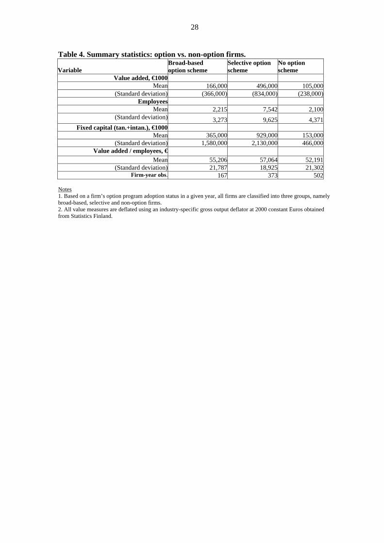
Table 4 presents the key variables grouped by a firm’s option program adoption
status. We observe that option firms have higher value added, bigger labour forces and
they also use more fixed capital compared to firms without stock option schemes. For
example, the mean value added for selective scheme firms is 496 million euros,
whereas for broad-based firms it is 166 million euros and for non-option firms only 105
million euros. Table 4 also shows that large Finnish firms have preferred targeted
schemes to broad-based option schemes. Finally, the mean value added per employee is
about 3.4% higher in selective scheme firms than in broad-based firms (57,064 euros
compared to 55,205 euros).
[Table 4 about here]
4. Econometric Strategy
We test two key hypotheses, namely: (i) that firm-level productivity is expected
to be higher in option than in non-option firms; (ii) that the impact of options on firm
productivity is expected to be dependent upon whether the plan is broad-based or
selective. Our basic empirical strategy is to use a production function approach and
panel data estimators. First, we estimate a series of baseline fixed effects estimators by

15
assuming that all explanatory variables are strictly exogenous. Second, we estimate
dynamic panel data GMM estimators to account for the potential endogeneity of a
firm’s decisions on inputs and option schemes. The following issues have influenced
the specific empirical strategy we adopt.
First, we assume a Cobb-Douglas form of technology, since it has been used
frequently in the related literature such as the evaluation of the effects of ESOPs on
firm productivity (e.g. Jones and Kato, 1995) and when analysing the effects of stock
options on firm performance (e.g. Conyon and Freeman, 2004.) Second, although the
Cobb-Douglas functional form is more restrictive than other functional forms such as
the translog, we prefer the Cobb-Douglas production function since, when accounting
for endogeneity of inputs and options in GMM models, the instrument matrix Zi may
become sizeable under the translog specification, thereby biasing estimates in finite
samples.12 Third, we assume that option schemes may only have a direct impact on firm
productivity.13 Fourth, since we do not have information on the detailed terms of option
schemes, such as the exercise prices of options, we must bypass potentially important
matters surrounding this issue.14
There are two reasons for using the fixed effects estimator in our baseline
estimates. In part this is pragmatic – we use the fixed effects estimator because it has
been used in the previous studies. For example, the estimator has been used in assessing
the productivity effects of ESOPs (e.g. Jones and Kato, 1995) and stock options (e.g.
Conyon and Freeman, 2004). Second, as is well known, firm fixed effects allow us to
control for unobserved time-invariant differences in firms, such as managerial ability,
employee quality and organization structure. We denote a firm’s production function
by , which relates firm value added(.)f 15 at time t, i.e. , to inputs used in production
and control variables:
itva
16
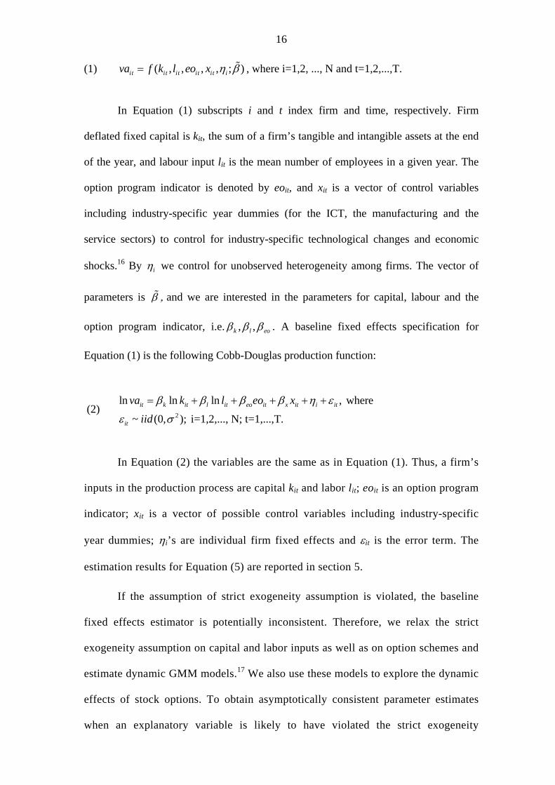
(1) ( , , , , ; )it it it it it iva f k l eo x η β= , where i=1,2, ..., N and t=1,2,...,T.
In Equation (1) subscripts i and t index firm and time, respectively. Firm
deflated fixed capital is kit, the sum of a firm’s tangible and intangible assets at the end
of the year, and labour input lit is the mean number of employees in a given year. The
option program indicator is denoted by eoit, and xit is a vector of control variables
including industry-specific year dummies (for the ICT, the manufacturing and the
service sectors) to control for industry-specific technological changes and economic
shocks.16 By iη we control for unobserved heterogeneity among firms. The vector of
parameters is β , and we are interested in the parameters for capital, labour and the
option program indicator, i.e. , ,k l eoβ β β . A baseline fixed effects specification for
Equation (1) is the following Cobb-Douglas production function:
(2) 2
ln ln ln , where
~ (0, ); i=1,2,..., N; t=1,...,T.it k it l it eo it x it i it
it
va k l eo x
iid
β β β β η ε
ε σ
= + + + + +
In Equation (2) the variables are the same as in Equation (1). Thus, a firm’s
inputs in the production process are capital kit and labor lit; eoit is an option program
indicator; xit is a vector of possible control variables including industry-specific
year dummies; ηi’s are individual firm fixed effects and εit is the error term. The
estimation results for Equation (5) are reported in section 5.
If the assumption of strict exogeneity assumption is violated, the baseline
fixed effects estimator is potentially inconsistent. Therefore, we relax the strict
exogeneity assumption on capital and labor inputs as well as on option schemes and
estimate dynamic GMM models.17 We also use these models to explore the dynamic
effects of stock options. To obtain asymptotically consistent parameter estimates
when an explanatory variable is likely to have violated the strict exogeneity
17
assumption, we estimate single equation GMM estimators18 by assuming the
following dynamic model:
(3) , 1 _1 , 1 1 , 1
2
ln ln ln ln ln ln
, where ; ~ iid(0, ); i=1,2,...,N; t=2,3,...,T. it va i t k it k i t l it l i t eo it
x it it it i it it
va va k k l l eo
x v v
β β β β β β
β ε ε η σ− − −= + + + + +
+ + = +−
In Equation (3) all variables correspond to those in equation (2). The
presence of individual effects ηi in the error term εit implies that the lagged
dependent variable vai,t-1 is positively correlated with εit. Thus, at least in large
samples with serially uncorrelated error terms vit, it can be shown that the OLS level
estimator for vaβ is inconsistent. Furthermore, the omitted variable literature
implies that the OLS level estimator for vaβ is biased upward in large samples (see,
e.g. Bond, 2002).
The fixed effects estimator (the within group estimator) removes this
inconsistency by transforming each variable to be its deviation from its firm mean.
However, if the number of time periods is small, the within group transformation
introduces a non-negligible negative correlation between a transformed lagged value
added vai,t-1 and a transformed error term vit. This result indicates that, at least in
large samples (N large), the fixed effects estimator for vaβ is biased downward (see,
e.g. Bond, 2002).
The fact that the OLS level estimator for Equation (3) is likely to be biased
upwards and the fixed effects estimator is likely to be biased downwards can be
useful information in assessing whether an estimator is consistent. In other words, a
consistent estimator would lie between the OLS level and the fixed effects
estimator. If we do not observe this pattern or an estimator is close to either the OLS
18
level or the fixed effects estimator, we might suspect severe finite sample bias or
inconsistency (see, e.g. Bond, 2002).
We follow a dynamic panel data GMM estimation strategy and allow
explanatory variables to be correlated with the individual effects ηi, since we
exclude these effects from Equation (3) by a first-difference transformation:
(4) , 1 _1 , 1
_1 , 1
ln ln ln ln ln
ln ,
where 1; i=1,2,...N; t=3,4,...T.
it va i t k it k i t l it
l i t eo it x it it
va
va va k k l
l eo x v
β β β β
β β β
β
− −
−
∆ = ∆ + ∆ + ∆ + ∆
+ ∆ + ∆ + ∆ + ∆
<
In Equation (4) we assume that the initial conditions are predetermined,
i.e. they are uncorrelated with the subsequent error terms
1iva
, 2,3,...,itv t T= and that
the error term is serially uncorrelated. We then apply the lagged levels of
dated at t-2 and t-3 as instruments for the corresponding first-differenced
variables.
itv
, 1i tva −
To account for potential endogeneity of inputs and options in equation (4),
we proceed in two steps. In the first stage, we assume that only labour and capital
inputs are endogenous variables. In the second stage, we also assume that option
schemes are endogenous (as well as the input variables.) When addressing the
potential endogeneity of capital and labour inputs, we assume that are
predetermined and use the lagged levels of dated at t-1 and t-2 as
instruments for the corresponding first-differenced variables. In other words, we
assume that there is no contemporaneous correlation between the inputs and the
error term , but that the inputs may be correlated with
itk itl ,it itk l
and it itk l
itv , 1i tv − and earlier shocks.19
To address endogeneity of option schemes, we treat the dilution option program
19
indicator as predetermined.,i teo 20 Then we use the once lagged variable, denoted t-1,
as an instrument for the corresponding first-differenced option program variables.
By accepting the moment condition restrictions above, we may construct an
instrument variable matrix Zi, where the lagged levels of explanatory variables are
used as instruments for the corresponding first-differenced variables.21 We follow
the terminology suggested by Bond (2002) and call these estimators the differenced
GMM estimators. As an extended estimator we apply the system GMM estimator22
by also assuming that the levels of explanatory variables, i.e. and , are
uncorrelated with individual effects η
,it itk l ,i teo
i and predetermined with respect to the error
term .itv 23 Thus we use lagged first-differences of and as instruments for
the GMM level equations. The estimation results for the differenced and the system
GMM estimators are separately reported in section 5, under both assumptions
concerning endogeneity.
, ,,i t i tk l ,i teo
5. Empirical Results
Table 5 reports the baseline contemporaneous fixed effects estimates for a
Cobb-Douglas production function during 1992-2002.24 The estimator deviates from
the standard fixed effects estimator in that we have specified a first-order
autocorrelation process in the residuals. This is the preferred estimation approach, since
the autocorrelation tests strongly indicates that the disturbance term is first-order
autoregressive.25
Three main conclusions emerge from Table 5. First, the estimates for capital
and labor are highly significant in columns (1)–(4). The baseline elasticity of capital
input is close to 0.15, whereas for labor it is about 0.62.26 Second, in columns (1) and
(2), where our option program indicator is the presence of a plan, we do not find
statistically significant evidence of contemporaneous association between options and

20
firm productivity. In column (1) the parameter estimate for the option program
indicator is 0.002, but it is statistically insignificant. In column (2) the signs of
parameters differ between selective and broad-based indicators. The selective scheme
estimate is 0.015 and the broad-based scheme -0.028. However, both are statistically
insignificant. Third, in columns (3) and (4), where our option program indicator is the
size of a plan, we find statistically significant evidence of contemporaneous association
between selective schemes and firm productivity (at the 10% level.) The parameter
estimate for selective schemes is 0.84, whereas for broad-based schemes it is
statistically insignificant -0.256. The mean dilution for selective schemes is 0.0286
indicating, on average, a 2.4% effect on firm productivity (0.0286*0.84=0.024).
[Table 5 about here]
Tables 6-8 show estimation results for the OLS level, the fixed effects, the
differenced GMM and the system GMM estimators for a Cobb-Douglas production
function.27 The reported GMM estimates are based on the two-step GMM estimator
with heteroskedastic-consistent asymptotic standard errors.28 We also perform a finite-
sample correction proposed by Windmeijer (2000), since simulation studies have
shown that these standard errors are downward biased.29 For all test statistics, we rely
on the two-step GMM estimator.
In Table 6 we relax the strict exogeneity assumptions on inputs. Our program
indicators are dummy variables, i.e. we measure the presence of a plan. The following
key findings emerge from Table 6. First, the OLS level parameter estimates for vat-1 in
columns (1) and (2) are substantially higher than the fixed effects estimates in columns
(3) and (4). As noted earlier, a consistent GMM estimator would lie between these two
estimators. Unfortunately we find that the differenced GMM estimates for vat-1 in
columns (5) and (6) are below the fixed effects estimates. Thus we suspect severe finite

21
sample bias or inconsistency which, in this case, is likely to be associated with weak
instruments for individual series that are highly time persistent.30 Another indication of
inconsistency is that the differenced GMM parameter estimates for capital inputs
reported in columns (5) and (6) are about twice as large as the OLS level and the fixed
effects estimates reported in columns (1)-(4).
Second, Table 6 suggests that the estimates for the presence of a plan are
statistically insignificant. In our preferred specifications, reported in columns (7) and
(8), where we have controlled for simultaneity of inputs by treating them as
predetermined, the signs of the option and selective scheme indicators are positive, but
the coefficient for the broad-based scheme indicator is negative. In sum, we do not find
statistical evidence of a contemporaneous association between option programs and
firm productivity.
Third, the system GMM parameter estimates using a lagged dependent variable
and reported in columns (7) and (8) are lower than the OLS level estimates but higher
than the fixed effects estimates. This finding indicates that the system GMM estimator
is likely to be consistent, at least for the lagged dependent variable.
Fourth, the autocorrelation tests, namely m1 and m2 reported in columns (7)
and (8), provide support for the system GMM estimator. The tests indicate significant
negative autocorrelation in the first-differenced residuals but not in the second-order
residuals. This is exactly how it should be, if the disturbances are serially uncorrelated,
indicating that the key assumption for the consistency of the system GMM estimator is
fulfilled. Moreover, the Sargan test clearly accepts the validity of instruments in
columns (5)-(8).
[Table 6 about here]

22
Next we focus on the endogeneity of an option program, since that may be
driving the baseline fixed effects estimates reported in Table 6. The findings reported in
Table 7 are based on a program’s size indicator31, but otherwise the estimation
approach is similar to that underlying the findings presented in Table 6. Since the OLS
level and the fixed effects estimates for the lagged dependent variable, the capital and
labor inputs are almost the same in both the tables, we do not discuss these findings any
further.
The following key findings emerge from Table 7. First, the fixed effect estimate
for selective programs reported in column (4) support the positive association, reported
previously in Table 6. Now the parameter estimate is 0.73 and it is statistically
significant at the 10% level. The mean dilution for selective schemes is 0.0286
indicating, on average, a 2.1% effect on firm productivity (0.0286*0.73=0.021). Note,
however, that the fixed effects findings in columns (3) and (4) are based on the
assumption that the explanatory variables are strictly exogenous.
Second, the system GMM estimators in columns (7)-(10) suggest that, after
controlling for potential endogeneity of the explanatory variables, all the estimated
option dilution indicators are found to be statistically insignificant. In columns (7) and
(8), where we have controlled for simultaneity of capital and labor inputs by treating
them as predetermined, the signs of all indicators are positive. In columns (9) and (10)
we also treat the dilution indicators as predetermined (to control for simultaneity), but
even then we do not find any evidence that is statistically significant that programs can
be associated with firm productivity. The parameter estimate for the selective scheme
reported in column (10) is now about one third as large (0.25) as the statistically
significant fixed effects estimate of 0.73 reported in column (4). The parameter
estimates for the broad-based dilution indicator (column 10) is -0.542. In sum, after
controlling for endogeneity, at conventional levels of statistical significance, we do not

23
find any evidence that option programs affect firm productivity. This conclusion holds
even in estimates that distinguish selective and broad-based option schemes.32
[Table 7 about here]
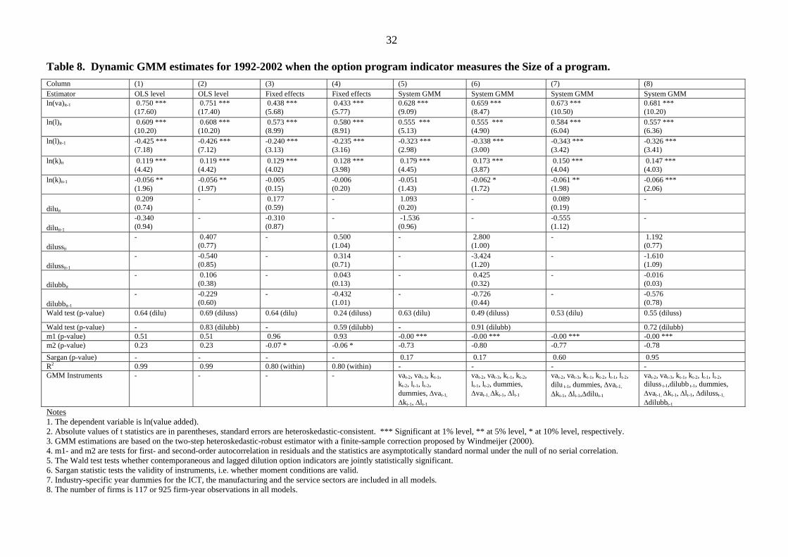
In Table 8 we expand our investigation to account for the dynamic effects of
option programs, since a stock option program typically spans several years. Hence the
effect on productivity may be realized with a lag. To account for dynamics we keep all
the assumptions used in the models reported in Table 7, but in Table 8 we report
estimates that use both contemporaneous and once lagged program indicators. As an
option program indicator we use the size of a plan. A Wald test is used to determine
whether contemporaneous and lagged indicators are jointly zero. We first estimate the
OLS level and the fixed effects models in columns (1)-(4), thereafter the system GMM
estimators in columns (5)-(8).33 In columns (5) and (6) we treat capital and labor inputs
as predetermined, and in columns (7) and (8), besides capital and labor, we also treat
the program indicator as predetermined.
The key finding is that we do not find convincing statistical evidence of an
association between option programs and firm productivity. The evidence for a
selective scheme having positive effects on productivity when using fixed effects
estimators and reported in Tables 5 and 7, is not supported in the dynamic models.
While the sum of contemporaneous and lagged parameter estimates of selective
schemes is 0.81, they are jointly statistically insignificant (p-value 0.24). Also, the
system GMM estimates for program indicators are all found to be statistically
insignificant.

24
6. Conclusions and Implications
In this paper we assemble new panel data for all Finnish publicly listed firms
during a relatively long period, namely 1992-2002. Our data enable us to distinguish
different types of option plans and to seriously address issues of endogeneity
concerning options and inputs. Consequently we are able to see if previous findings that
are based mainly on evidence generated using data that are less representative and for
shorter time periods are sustained.
We proceed by estimating Cobb-Douglas production functions with three
different option program indicators. These measures reflect the presence or absence of
an option scheme, the size of the scheme and whether the scheme is selective or broad
based. Furthermore, the long panel nature of our data allows us to estimate dynamic
panel data models with a GMM estimator and thus address the potentially important
issue of endogeneity of inputs and options.
The most important finding, yielded almost consistently in diverse
specifications, is a statistically insignificant association between option programs and
firm productivity. This result is exceptionally robust for broad-based schemes and is
independent of what option program indicator is used in estimations. As such our
findings are consistent with those who hypothesize that the performance impact of
options will be limited because of reasons such as free-rider problems (e.g. Oyer,
2004), accounting myopia (e.g. Hall and Murphy, 2003) or line-of-sight arguments (e.g.
Vroom, 1995). As such our results are consistent with much of the financial literature
that does not find evidence of a link between options and business performance (e.g.
Hall and Murphy, 2003.)
For selective programs, however, findings are less consistent. In our baseline
fixed effects estimates we find a statistically significant productivity impact that is
between 2.1-2.4%. Since most selective plans are allocated to executives and/or key

25
employees, this finding also provides support for the line-of-sight argument – rewards
based on performance can only be motivating if the action of employees can influence
the measures on which the performance-pay is based. Equally, this evidence does not
support those who stress managerial rent-seeking as the principal reason for introducing
selective option plans. However in models where endogeneity is accounted for, we do
not find any strong evidence of a link with firm productivity. Similarly in models that
investigate the dynamics of selective programs, no association between selective
options and firm productivity is found.
In sum, our findings differ in important ways from earlier findings that are
based on less rigorous methods and use more limited data. In particular, our findings do
not provide strong support for hypotheses of a positive association between option
schemes and firm productivity.

26
Table 1. The evolution of Finnish stock option plans 1992-2002. Year (1)
# of firms in Helsinki Stock Exchanges
(2) # of new option plans
(3) #of new broad-based option plans
(4) # of firms having option plan
(5) # of firms having broad-based option plan
1992 65 1 0 11 (16.9%)
2 (3.1%)
1993 60 6 1 15 (25.0%)
2 (3.3%)
1994 68 21 2 34 (50%)
3 (5.0%)
1995 74 7 1 38 (51.4%)
3 (4.1%)
1996 73 9 3 36 (49.3%)
6 (8.2%)
1997 1151) 221) 41) 461)
(40.0%) 71)
(6.1%) 1998 119 47 17 69
(58.0%) 21 (17.6%)
1999 137 42 23 91 (66.4%)
36 (26.3%)
2000 150 61 30 113 (75.3%)
54 (36.0%)
2001 145 33 11 112 (77.2%)
54 (37.2%)
2002 137 33 6 101 (73.7%)
49 (35.8%)
Total 282 101 Notes: 1. Before 1997 data are only for main list firms. From 1997 onwards, the data also include the New Market and the Investor list firms. 2. Note that stock option data in Table 2 also includes firms that have less than four consecutive year observations. 3. Source: Helsinki School of Economics, Alexander Corporate Finance and authors’ calculations.

27
Table 2. The pattern of firm-level panel data, 1992-2002.
Freq. Percent Cumulative Pattern 40 34.2 34.2 11111111111
21 18.0 52.1 01111111111
12 10.3 62.4 00111111111
10 8.6 70.9 00001111111
7 6.0 76.9 00000111111
4 3.4 80.3 00000011111
3 2.6 82.9 00000001111
3 2.6 85.5 00011111111
3 2.6 88.0 01111111110
14 12.0 100.0 (other patterns)
117 100 Notes 1. The last column describes the pattern of data: 1 means we have an observation for this year, 0 we do not. The first digit (0 or 1) in the pattern column is year 1992. Thus the first row indicates that in 40 cases we have data for all years, whereas the second row indicates that in 21 cases there is no data for 1992 but that data are available in all other years.
Table 3. Summary statistics.
Variable
Name
Firm- year obs Mean Std. Dev.
l Employees 1042 4,066 7,123 k Fixed capital (tan.+intan.), €1000 1042 464,000 1,500,000q Value added, €1000 1042 255,000 574,000
Dilu* Potential dilution in the range of (0,1); a proxy of option program size 531 0.0547 0.0450
Diluss* Potential dilution for selective stock option programs 364 0.0286 0.0285
Dilubb* Potential dilution for broad-based stock option programs 167 0.0900 0.0533
Opt Option program dummy 1042 0.5182 0.4999 Ssopt Selective option program dummy 1042 0.3580 0.4796 Bbsopt Broad-based option program dummy 1042 0.1603 0.3670 Ln(l) Natural logarithm of employees 1042 7.10 1.62 Ln(k) Natural logarithm of deflated fixca 1042 17.95 2.07 Ln(q) Natural logarithm of deflated sales 1042 17.95 1.72 Notes 1. All value measures are deflated using an industry-specific gross output deflator at 2000 constant Euros obtained from Statistics Finland. 2. * Summary statistics for dilu, diluss and dilubb variables are only for those firms that have a stock option program. 3. The total number of firm-year observations is 1042 and data are for 117 firms.
28
Table 4. Summary statistics: option vs. non-option firms. Variable
Broad-based option scheme
Selective option scheme
No option scheme
Value added, €1000 Mean 166,000 496,000 105,000
(Standard deviation) (366,000) (834,000) (238,000)Employees
Mean 2,215 7,542 2,100(Standard deviation) 3,273 9,625 4,371
Fixed capital (tan.+intan.), €1000 Mean 365,000 929,000 153,000
(Standard deviation) 1,580,000 2,130,000 466,000Value added / employees, €
Mean 55,206 57,064 52,191(Standard deviation) 21,787 18,925 21,302
Firm-year obs. 167 373 502 Notes 1. Based on a firm’s option program adoption status in a given year, all firms are classified into three groups, namely broad-based, selective and non-option firms. 2. All value measures are deflated using an industry-specific gross output deflator at 2000 constant Euros obtained from Statistics Finland.

29
Table 5. Baseline fixed effects estimates: Cobb-Douglas production functions, 1992-2002.
Column (1) (2) (3) (4) ln(k)it 0.150 ***
(6.38) 0.151 *** (6.39)
0.150 *** (6.38)
0.150 *** (6.37)
ln(l)it 0.617 *** (15.26)
0.621 *** (15.32)
0.615 *** (15.05)
0.619 *** (15.18)
optit 0.002 (0.06)
ssoptit 0.015 (0.56)
bbsoptit -0.028 (0.81)
diluit 0.076 (0.24)
dilussit 0.840 * (1.79)
dilubbit -0.256 (0.73)
Firm-year obs. 925 925 925 925
Firms 117 117 117 117 Baltagi-Wu LBI1) 1.32 1.32 1.32 1.32 Modified Bhargava et al.1)
0.94 0.94 0.94 0.94
R2 within 0.61 0.61 0.61 0.62
Notes 1. The dependent variable is ln(value added). 2. The estimator is a modified fixed effects estimator -xtregar-, where the disturbance is first-order autoregressive. 3. Absolute values of t statistics in parentheses. *** Significant at 1% level, ** at 5% level, * at 10% level, respectively. 4. Opt is a dummy variable for the presence of an option program, ssopt is a dummy variable for the presence of a selective program and bbsopt is a dummy variable for the presence of a broad-based option program. Diluss is an interaction variable between potential dilution and ssopt dummy. Dilubb is an interaction variable between potential dilution and bbsopt dummy. 5. Industry-specific year dummies for the ICT, the manufacturing and the service sectors are included in all models. 6. 1) The tests are based on the standard fixed effects models without modelling first-order autoregression. Baltagi-Wu LBI is the Baltagi-Wu (1999) locally best invariant test statistic for ρ = 0. If a test statistic is far below 2, it is an indication of positive serial correlation. Modified Bhargava et al. (1982) also test if ρ =0. If the test statistic is significantly different from zero, we have serial correlation. The tests indicate serial correlation supporting the modified fixed effects estimator.
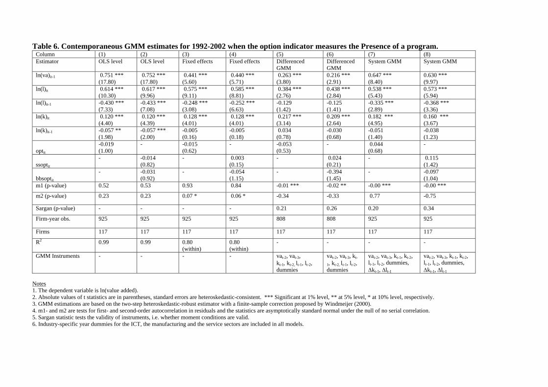
Table 6. Contemporaneous GMM estimates for 1992-2002 when the option indicator measures the Presence of a program. Column
(1) (2) (3) (4) (5) (6) (7) (8) Estimator OLS level OLS level Fixed effects Fixed effects Differenced
GMM Differenced GMM
System GMM System GMM
ln(va)it-1 0.751 *** (17.80)
0.752 *** (17.80)
0.441 *** (5.60)
0.440 *** (5.71)
0.263 *** (3.80)
0.216 *** (2.91)
0.647 *** (8.40)
0.630 *** (9.97)
ln(l)it 0.614 *** (10.30)
0.617 *** (9.96)
0.575 *** (9.11)
0.585 *** (8.81)
0.384 *** (2.76)
0.438 *** (2.84)
0.538 *** (5.43)
0.573 *** (5.94)
ln(l)it-1 -0.430 *** (7.33)
-0.433 *** (7.08)
-0.248 *** (3.08)
-0.252 *** (6.63)
-0.129 (1.42)
-0.125 (1.41)
-0.335 *** (2.89)
-0.368 *** (3.36)
ln(k)it 0.120 *** (4.40)
0.120 *** (4.39)
0.128 *** (4.01)
0.128 *** (4.01)
0.217 *** (3.14)
0.209 *** (2.64)
0.182 *** (4.95)
0.160 *** (3.67)
ln(k)it-1 -0.057 ** (1.98)
-0.057 *** (2.00)
-0.005 (0.16)
-0.005 (0.18)
0.034 (0.78)
-0.030 (0.68)
-0.051 (1.40)
-0.038 (1.23)
optit
-0.019 (1.00)
- -0.015(0.62)
- -0.053(0.53)
- 0.044(0.68)
-
ssoptit
- -0.014(0.82)
- 0.003(0.15)
- 0.024(0.21)
- 0.115(1.42)
bbsoptit
- -0.031(0.92)
- -0.054(1.15)
- -0.394(1.45)
- -0.097(1.04)
m1 (p-value) 0.52 0.53 0.93 0.84 -0.01 *** -0.02 ** -0.00 *** -0.00 ***
m2 (p-value) 0.23 0.23 0.07 * 0.06 * -0.34 -0.33 0.77 -0.75
Sargan (p-value) - - - - 0.21 0.26 0.20 0.34
Firm-year obs. 925 925 925 925 808 808 925 925
Firms 117 117 117 117 117 117 117 117
R2 0.99
0.99
0.80 (within)
0.80 (within)
- - - -
GMM Instruments - - - - vat-2, vat-3, kt-1, kt-2, lt-1, lt-2, dummies
vat-2, vat-3, kt-
1, kt-2, lt-1, lt-2, dummies
vat-2, vat-3, kt-1, kt-2, lt-1, lt-2, dummies, ∆kt-1, ∆lt-1
vat-2, vat-3, kt-1, kt-2, lt-1, lt-2, dummies, ∆kt-1, ∆lt-1
Notes 1. The dependent variable is ln(value added). 2. Absolute values of t statistics are in parentheses, standard errors are heteroskedastic-consistent. *** Significant at 1% level, ** at 5% level, * at 10% level, respectively. 3. GMM estimations are based on the two-step heteroskedastic-robust estimator with a finite-sample correction proposed by Windmeijer (2000). 4. m1- and m2 are tests for first- and second-order autocorrelation in residuals and the statistics are asymptotically standard normal under the null of no serial correlation. 5. Sargan statistic tests the validity of instruments, i.e. whether moment conditions are valid. 6. Industry-specific year dummies for the ICT, the manufacturing and the service sectors are included in all models.

31
Table 7. Contemporaneous GMM estimates for 1992-2002 when the option indicator measures the Size of a program.
Notes
Column (1) (2) (3) (4) (5) (6) (7) (8) (9) (10)Estimator OLS level OLS level Fixed effects Fixed effects Differenced
GMM Differenced
GMM System GMM System GMM System GMM System GMM
ln(va)it-1 0.751 *** (17.70)
0.752 *** (17.60)
0.440 *** (5.61)
0.438 *** (5.72)
0.266 *** (3.89)
0.227 *** (3.13)
0.653 *** (8.83)
0.657 *** (8.94)
0.682 *** (10.50)
0.681 *** (10.20)
ln(l)it 0.610 *** (10.20)
0.609 *** (10.30)
0.572 *** (9.03)
0.577 *** (8.97)
0.416 *** (2.48)
0.601 *** (2.75)
0.550 *** (5.17)
0.552 *** (5.32)
0.578 *** (5.85)
0.571 *** (5.48)
ln(l)it-1 -0.428 *** (7.26)
-0.428 *** (7.23)
-0.244 *** (3.10)
-0.242 *** (3.13)
-0.141 (1.48)
-0.115 (1.48)
-0.339 *** (2.97)
-0.341 *** (3.08)
-0.351 *** (3.28)
-0.340 *** (3.86)
ln(k)it 0.119 *** (4.40)
0.119 *** (4.40)
0.128 *** (4.02)
0.128 *** (3.98)
0.236 *** (2.68)
0.201 *** (2.50)
0.181 *** (4.99)
0.179 *** (4.71)
0.152 *** (4.31)
0.149 *** (3.20)
ln(k)it-1 -0.056 ** (1.96)
-0.056 ** (1.96)
-0.001 (0.16)
-0.007 (0.21)
0.027 (0.73)
-0.006 (0.12)
-0.057 (1.60)
-0.060 * (1.72)
-0.063 ** (1.98)
-0.072 ** (1.99)
diluit
-0.059 (0.30)
- -0.017(0.05)
- -1.948 -(1.20)
0.161(0.20)
- -0.381(0.56)
-
dilussit
- 0.019(0.07)
- 0.728 * (1.72)
- 4.030(1.07)
- 0.859(0.55)
- 0.247(0.29)
dilubbit
- -0.076(0.34)
- -0.276(0.74)
- -3.462(1.61)
- 0.061 (0.08)
- -0.542(1.07)
m1 (p-value) 0.51 0.51 -0.96 0.89 -0.01 *** 0.01 *** -0.00 *** -0.00 *** -0.00 *** -0.00 *** m2 (p-value) 0.22 0.22 -0.07 * -0.06 * 0.51 -0.59 -0.76 -0.76 -0.79 -0.80 Sargan (p-value) - - - - 0.26 0.36 0.19 0.21 0.64 0.84 Firm-year obs. 925 925 925 925 808 808 925 925 925 925Firms 117 117 117 117 117 117 117 117 117 117R2 0.99 0.99 0.80 (within) 0.80 (within) - - - - - - GMM Instruments - - - - vat-2, vat-3,
kt-1, kt-2, lt-1, lt-2, dummies
vat-2, vat-3, kt-1, kt-2, lt-1, lt-2, dummies
vat-2, vat-3, kt-1, kt-2, lt-1, lt-2, dummies, vat-1, ∆kt-1, ∆lt-1
vat-2, vat-3, kt-1, kt-2, lt-1, lt-2, dummies,∆vat-
1, ∆kt-1, ∆lt-1
vat-2, vat-3, kt-1, kt-
2, lt-1, lt-2, dilu t-1, dummies,∆vat-1, ∆kt-1, ∆lt-1, ∆dilut-1
vat-2, vat-3, kt-1, kt-2, lt-1, lt-2, diluss t-1, dilubb t-1, dummies,∆vat-1, ∆kt-1, ∆lt-1, ∆dilusst-1, dilubbt-1
1. The dependent variable is ln(value added). 2. Absolute values of t statistics are in parentheses, standard errors are heteroskedastic-consistent. *** Significant at 1% level, ** at 5% level, * at 10% level, respectively. 3. GMM estimations are based on the two-step heteroskedastic-robust estimator with a finite-sample correction proposed by Windmeijer (2000). 4. m1- and m2 are tests for first- and second-order autocorrelation in residuals and the statistics are asymptotically standard normal under the null of no serial correlation. 5. Sargan statistic tests the validity of instruments, i.e. whether moment conditions are valid. 6. Industry-specific year dummies for the ICT, the manufacturing and the service sectors are included in all models.
32
Table 8. Dynamic GMM estimates for 1992-2002 when the option program indicator measures the Size of a program.
Notes
Column (1) (2) (3) (4) (5) (6) (7) (8)Estimator OLS level OLS level Fixed effects Fixed effects System GMM System GMM System GMM System GMM ln(va)it-1 0.750 ***
(17.60) 0.751 *** (17.40)
0.438 *** (5.68)
0.433 *** (5.77)
0.628 *** (9.09)
0.659 *** (8.47)
0.673 *** (10.50)
0.681 *** (10.20)
ln(l)it 0.609 *** (10.20)
0.608 *** (10.20)
0.573 *** (8.99)
0.580 *** (8.91)
0.555 *** (5.13)
0.555 *** (4.90)
0.584 *** (6.04)
0.557 *** (6.36)
ln(l)it-1 -0.425 *** (7.18)
-0.426 *** (7.12)
-0.240 *** (3.13)
-0.235 *** (3.16)
-0.323 *** (2.98)
-0.338 *** (3.00)
-0.343 *** (3.42)
-0.326 *** (3.41)
ln(k)it 0.119 *** (4.42)
0.119 *** (4.42)
0.129 *** (4.02)
0.128 *** (3.98)
0.179 *** (4.45)
0.173 *** (3.87)
0.150 *** (4.04)
0.147 *** (4.03)
ln(k)it-1 -0.056 ** (1.96)
-0.056 ** (1.97)
-0.005 (0.15)
-0.006 (0.20)
-0.051 (1.43)
-0.062 * (1.72)
-0.061 ** (1.98)
-0.066 *** (2.06)
diluit
0.209 (0.74)
- 0.177(0.59)
- 1.093(0.20)
- 0.089(0.19)
-
diluit-1
-0.340 (0.94)
- -0.310(0.87)
- -1.536(0.96)
- -0.555(1.12)
-
dilussit
- 0.407(0.77)
- 0.500(1.04)
- 2.800(1.00)
- 1.192(0.77)
dilussit-1
- -0.540(0.85)
- 0.314(0.71)
- -3.424(1.20)
- -1.610(1.09)
dilubbit
- 0.106 (0.38)
- 0.043 (0.13)
- 0.425 (0.32)
- -0.016(0.03)
dilubbit-1
- -0.229(0.60)
- -0.432(1.01)
- -0.726(0.44)
- -0.576(0.78)
Wald test (p-value) 0.64 (dilu) 0.69 (diluss) 0.64 (dilu) 0.24 (diluss) 0.63 (dilu) 0.49 (diluss) 0.53 (dilu) 0.55 (diluss)
Wald test (p-value) - 0.83 (dilubb) - 0.59 (dilubb) - 0.91 (dilubb) 0.72 (dilubb) m1 (p-value) 0.51 0.51 0.96 0.93 -0.00 *** -0.00 *** -0.00 *** -0.00 *** m2 (p-value) 0.23 0.23 -0.07 * -0.06 * -0.73 -0.80 -0.77 -0.78 Sargan (p-value) - - - - 0.17 0.17 0.60 0.95 R2 0.99 0.99 0.80 (within) 0.80 (within) - - - - GMM Instruments - - - - vat-2, vat-3, kt-1,
kt-2, lt-1, lt-2, dummies, ∆vat-1,
∆kt-1, ∆lt-1
vat-2, vat-3, kt-1, kt-2, lt-1, lt-2, dummies, ∆vat-1, ∆kt-1, ∆lt-1
vat-2, vat-3, kt-1, kt-2, lt-1, lt-2, dilu t-1, dummies, ∆vat-1,
∆kt-1, ∆lt-1,∆dilut-1
vat-2, vat-3, kt-1, kt-2, lt-1, lt-2, diluss t-1,dilubb t-1, dummies, ∆vat-1, ∆kt-1, ∆lt-1, ∆dilusst-1,
∆dilubbt-1
1. The dependent variable is ln(value added). 2. Absolute values of t statistics are in parentheses, standard errors are heteroskedastic-consistent. *** Significant at 1% level, ** at 5% level, * at 10% level, respectively. 3. GMM estimations are based on the two-step heteroskedastic-robust estimator with a finite-sample correction proposed by Windmeijer (2000). 4. m1- and m2 are tests for first- and second-order autocorrelation in residuals and the statistics are asymptotically standard normal under the null of no serial correlation. 5. The Wald test tests whether contemporaneous and lagged dilution option indicators are jointly statistically significant. 6. Sargan statistic tests the validity of instruments, i.e. whether moment conditions are valid. 7. Industry-specific year dummies for the ICT, the manufacturing and the service sectors are included in all models. 8. The number of firms is 117 or 925 firm-year observations in all models.
References Alchian, Armen, and Harold Demsetz (1972). “Production, Information Costs, and Economic Organisation.” American Economic Review, 62, 777-795. Arellano, Manuel, and Stephen Bond (1991). “Some Tests of Specification for Panel Data: Monte Carlo Evidence and an Application to Employment Equations.” Review of Economic Studies, 58, 277-297. Arrelano, Manuel, and Olympia Bover (1995). “Another Look at the Instrumental Variables Estimation of Error-Components Model.” Journal of Econometrics, 68, 29-51. Arellano, Manuel (2003). Panel Data Econometrics. Oxford University Press. Baron, James N., and David M. Kreps (1999). Strategic Human Resources: Frameworks for General Managers. New York, Wiley. Bebchuk, Lucian A., and Jesse M. Fried (2003). “Executive Compensation as an Agency Problem.” Journal of Economic Perspectives, 17, 71-92. Blasi, Joseph, Douglas Kruse, and Aaron Bernstein (2003). In the Company of Owners: The Truth About Stock Options and Why Every Employee Should Have Them. New York, Basic Books. Blundell, Richard W., and Stephen Bond (1998). “Initial Conditions and Moment Restrictions in Dynamic Panel Data Models.” Journal of Econometrics, 87, 115-143. Blundell, Richard W., Stephen Bond, and Frank Windmeijer (2000). “Estimation in Dynamic Panel Data Models: Improving on the Performance of the Standard GMM Estimators.” In B. Baltagi (eds.), Nonstationary Panels, Panel Cointegration and Dynamic Panels, Advances in Econometrics 15, Amsterdam: JAI Press, Elsevier Science. Bond, Stephen (2002). “Dynamic Panel Data Models: A Guide to Micro Data Methods and Practice.” Portuguese Economic Journal, 1, 141-162. Bound, John, David A. Jaeger, and Regina M. Baker (1995). “Problems with Instrumental Variables Estimation when the Correlation between the Instruments and the Endogenous Explanatory Variables is Weak.” Journal of the American Statistical Association, 90, 443-450. Cable, John, and Nicholas Wilson (1990). “Profit-Sharing and Productivity: Some Further Evidence.” Economic Journal, 100 (401), 550-555. Conte, Michael, and Jan Svejnar (1988). “Productivity Effects of Worker Participation in Management, Profit-Sharing, Worker Ownership of Assets and Unionization in U.S. Firms.” International Journal of Industrial Organization, vol. 6, issue 1, 139-151. Conyon, Martin J., and Richard B. Freeman (2004). “Shared Modes of Compensation and Firm Performance: UK Evidence.” In Richard Blundell, David Card and Richard Freeman (eds.): Seeking a Premier League Economy, Chicago: University of Chicago Press.
34
Djankov, Simeon, and Peter Murrell (2002). “Enterprise Restructuring in Transition: A Quantitative Survey.” Journal of Economic Literature, 40 (3): 739-92. Drukker, David M. (2003): “Testing for Serial Correlation in Linear Panel-Data Models.” Stata Journal, (3)2, 168-177. Griliches, Zvi, and Jacques Mairesse (1998). “Production Functions: The Search for Identification.” Econometrics and Economic Theory in the Twentieth Century: The Ragnar Frisch Centennial Symposium, Cambridge University Press. Hall, Brian J. (1998). “The Pay to Performance Incentives of Executive Stock Options.” NBER Working Paper 6674. Hall, Brian J., and Kevin J. Murphy (2003). “The Trouble with Stock Options.” Journal of Economic Perspectives, 17, 49-70. Ikäheimo, Seppo, Anders Kjellman, Jan Holmberg, and Satu Jussila (2004). “Employee Stock Option Plans and Stock Market Reaction: Evidence from Finland.” European Journal of Finance, 10, 105-122. Ittner, Christopher D., Richard A Lambert, and David F. Larcker (2003). “The Structure and Performance of Equity Grants to Employees of New Economy Firms.” Journal of Accounting and Economics, 34, 89-127. Jones, Derek C., and Takao Kato (1995). “The Productivity Effects of Employee Stock-Ownership Plans and Bonuses: Evidence from Japanese Panel Data.” American Economic Review, 85, 391-414. Jones, Derek C., and Jeffrey Pliskin (1991). “The Effects of Worker Participation, Employee Ownership and Profit Sharing on Economics Performance.” In International Handbook of Participation in Organizations, eds. Raymond Russell, and Veljko Rus, vol. 2, Oxford University Press. Jones, Derek C., Panu Kalmi, and Mikko Mäkinen (2006). “The Determinants of Stock Option Compensation: Evidence from Finland. Industrial Relations, 45, 437-468. Kandel, Eugene, and Edward P. Lazear (1992). “Peer Pressure in Partnerships.” Journal of Political Economy, 100, 801-817. Kauhanen, Antti, and Hannu Piekkola (2002). “Profit Sharing in Finland: Earnings and Productivity Effects.” ETLA Discussion Paper 817. The Research Institute of the Finnish Economy. Kruse, Douglas L. (1992). “Profit Sharing and Productivity: Microeconomic Evidence from the United States.” Economic Journal, 102, 24-36. Kruse, Douglas L. (2002). “Research Evidence on the Prevalence and Effects of Employee Ownership.” Journal of Employee Ownership Law and Finance, 14, 65 – 90. Kumbhakar, Subal C., and Amy Dunbar (1993). “The Elusive ESOP- Productivity Link.” Journal of Public Economics, 52, 273-283.
35
Lebow, David, Louise Sheiner, Larry Slifman, and Martha Starr-McCleur (1998). “Recent Trends in Compensation Practices.” US Federal Reserve Board. Washington. Mäkinen, Mikko (2001): “Optiot – Suomalaisjohtajien uusi kannustin”. Title in English: Stock Options − The New Incentive of Finnish Executives. In Finnish with English Summary. B182, The Research Institute of Finnish Economy. Murphy, Kevin J. (1999). “Executive Compensation.” In Orley C. Ashenfelter and David Card (eds.): Handbook of Labor Economics, vol. 3B, Amsterdam, Elsevier, 2485-2563. Oyer, Paul (2004). “Why Do Firms Use Incentives That Have No Incentive Effects?” Journal of Finance, 59, 1619-1641. Pierce, Jon, Stephen A. Rubenfeld, and Susan Morgan (1991). “Employee Ownership: A Conceptual Model of Process and Effects.” Academy of Management Review, 16, 121-144. Rosen, Corey (2006). “The Future of Broad-Based Stock Options: What Research Tells Us”. In Panu Kalmi and Mark Klinedinst (eds.), Participation in the Age of Globalization and Information, Advances in the Economic Analysis of Participatory and Labor-Managed Firms, vol. 9. Rousseau, Denise M., and Zipi (2003). “Pieces of the Action: Ownership and the Changing Employment Relationship.” Academy of Management Review, 28, 553-570. Sesil, James C, Maya A. Kroumova, Joseph R. Blasi, and Douglas L. Kruse (2000). “Broad-Based Employee Options in the US: Do They Impact Company Performance?” Academy of Management Proceedings, HR:G1-G6. Sesil, James C, Maya A. Kroumova, Joseph R. Blasi, and Douglas L. Kruse (2002). “Broad-Based Employee Options in “New Economy” Firms: Company Performance Effects.” British Journal of Industrial Relations, 40, 273-295. Vroom, Victor H. (1995). Work and Motivation. Revised edition. San Fransisco: Jossey-Bass. Wadhwani, Sushil, and Martin Wall (1990). “The Effects of Profit-Sharing on Employment, Wages, Stock Returns and Productivity: Evidence from UK Micro-Data.” Economic Journal, 100, 1-17. Weeden, Ryan, Ed Carberry, and Scott Rodrick (1998). “Current Practices in Stock Option Plan Design.” National Center for Employee Ownership. Oakland, California. Weitzman, Martin L., and Douglas L. Kruse (1990). “Profit Sharing and Productivity.” In A. Blinder (ed.), Paying for Productivity. The Brookings Institution, Washington, 94-141. Windmeijer, Frank (2000). “Efficiency Comparisons for a System GMM Estimator in Dynamic Panel Data Models.” In R. D.H. Heijmans, D.S.G. Pollock and A. Satorra (eds.), Innovations in Multivariate Statistical Analysis, A Festschrift for Heinz Neudecker, Advanced Studies in Theoretical and Applied Econometrics, 36, Dordrecht: Kluwer Academic Publishers.

36
Endnotes
1 Earlier versions of this paper have benefited from comments by participants at the ASSA/ACES meeting in San Diego, January 2-5, 2004, the 12th IAFEP Conference in Halifax, July 8-10, 2004, the 16th EALE conference in Lisbon, September 9-11, 2004, the FPPE Industrial Organisation Workshop in Helsinki, December 9-10, 2004, and the EALE/SOLE World Conference in San Francisco, June 2-5, 2005. We are especially grateful to Kevin F. Hallock, Kari Hämäläinen, Pekka Ilmakunnas, Uwe Jirjahn, Jeffrey Pliskin and Otto Toivanen for their very helpful comments. Also we acknowledge Professor Seppo Ikäheimo and Alexander Corporate Finance for allowing us access to their databases on options in publicly traded Finnish companies, and to Mikael Katajamäki for his outstanding research assistance. We also thank Balance Consulting for financial statement data. Kalmi and Mäkinen gratefully acknowledge funding from the LIIKE-programme of the Academy of Finland. Kalmi also gratefully acknowledges financial support from the Marcus Wallenberg Foundation and the Helsinki School of Economics Research Foundation. In addition, Mäkinen thanks the Yrjö Jahnsson Foundation, the Helsinki School of Economics Research Foundation and the Foundation of Kluuvi for financial support. Support from the Research Institute of the Finnish Economy (ETLA) is gratefully acknowledged. 2 Mäkinen (2001) describes the evolution of stock option programs in Finland. Jones, Kalmi and Mäkinen (2006) study the determinants of option schemes adoption in Finland. They also summarise the evolution of options in Finland and discuss the institutional background in more detail. 3 One reason for the paucity of such studies is the lack of firm-level stock option data. For example, the S&P ExecuComp database contains only employee stock options grant values for the top five highest paid executives. However, financial economists have studied the links between stock option plans and appropriate accounting measures such as contemporaneous stock returns or stock market returns in the following year. Since our focus is on productivity, we do not comprehensively review such studies though we note that many finance studies do not find evidence of strong links between options and firm performance (e.g. Hall and Murphy, 2003.) For a broad review of pertinent empirical work see Rosen (2006). 4 These are part of a broader class of studies that employ an augmented production function methodology. For example, for a review of such work in investigating the impact of ownership forms on firm performance in transition economies, see Djankov and Murrell (2002). 5 However, we have included option schemes prior to the listing for such firms that enter the HEX before 2002. 6 This is done to provide the reader with a better understanding of the development and prevalence of option schemes in Finland. See more detailed evolution and institutional background description in Jones, Kalmi and Mäkinen (2006). 7 We omit 8 firms or 15 firm-year observations due to their having fewer than 4 consecutive observations. To utilize all possible firm-level financial information data we also collected data on income statements prior a firm’s listing on the Helsinki Stock Exchange.

37
8 Our classification is thus different from Kroumova et al. (2000; 2002), who use 50 % threshold as a criterion for broad-based schemes. Our data do not include this information, but have the important advantage of being derived from publicly reported sources that must be externally verifiable, rather than from confidential surveys. 9 We also interviewed Mr. Erkki Helaniemi, a partner in the investment bank Alexander Corporate Finance, who has been personally involved in setting up dozens of option schemes. He confirmed that there are dramatic differences in the participation rates for option schemes, depending on eligibility. 10 The first two are option program dummy variables, which measure the presence or absence of an option program. The dummy variable captures a program’s “introduction effect”: when an option program is adopted, a dummy variable switches from 0 to 1 shifting a linear production function immediately and without anticipation. This effect of an option plan on firm-level productivity is modelled as a constant over firms. The third measure is a proxy for the size of a program. 11 Unfortunately, we do not have information on stock option program details such as exercise prices to calculate Black-Scholes values. 12 When instrumenting inputs in a dynamic GMM estimation, the instrument matrix becomes substantially larger in the translog case. If the full set of instruments is used in a finite sample, this may bias estimates. 13 While this assumption substantially simplifies modelling, it may not be harmless. For example, the adoption of a scheme may not be less important than how a plan is actually implemented within a firm. Thus, if adoption is coupled with the introduction of new workplace practices, such as self-managed teams with some decision-making power, or increasing the number of regular employees meetings, the effects on firm productivity can be expected to differ than if the option scheme were to be introduced alone. Unfortunately, we do not have information on workplace practices besides options. 14 For example, presumably the terms of option schemes differ among firms. Thus, when an option scheme is substantially out of the money (i.e. the current stock price is substantially below the exercise price), options may not provide strong incentives for employees and managers to improve their performance. 15 On theoretical grounds firm value added is a preferable measure to sales, since value added does not include intermediate inputs that are purchased from other firms. 16 This decision is supported by the fact that the ICT sector experienced both boom and bust during 1997-2003. 17 Our decision to use a GMM estimator has been guided by the fact that we do not have suitable instrument variables for option schemes. 18 Besides these dynamic panel data GMM estimators, Maximum likelihood (ML) estimators have also been developed. Unfortunately, one drawback of the ML estimators is that different distributional assumptions of the initial conditions are needed in the estimation process to imply different likelihood functions. It follows that ML estimators may produce inconsistent estimate for the lagged dependent variable

38
(i.e. lnva,t-1), if an initial condition distribution, i.e. the distribution of vai1, is not the correct one. By contrast, the dynamic panel data GMM estimators do not need such a strong initial condition assumption. 19 This seems to be a reasonable assumption, since firms may not adjust their capital and labour inputs immediately on economic shocks within a year. For example, firms may be unaware as to whether a shock is permanent or temporary. 20 Since option plans typically are introduced publicly in early spring, a few weeks before the annual general meeting of shareholders, this seems to be a reasonable assumption. Therefore, a potential correlation is likely to be with a previous period rather than being contemporaneous. 21 For more on dynamic GMM estimators and constructing an instrument variable matrix see Arellano and Bond (1991), Arellano and Bover (1995), and Blundell and Bond (1998). 22 The benefit of using the system GMM estimator is that it is shown to be more efficient than the differenced GMM estimator in large samples. 23 To us the non-correlation seems more plausible approach than assuming that the first-differences of capital and labour are uncorrelated with individual effects ηi. 24 We use Stata/SE 9.1 for Windows statistical package in estimating the models of Table 5. 25 We also performed the modified Wald statistics to examine a groupwise heteroskedasticity in the residuals when estimating a standard fixed effects estimator. The statistics indicate a violation in assumption that the error term is homoskedastic. Thus, the modified Wald statistic indicates that the fixed effects estimator is not efficient, which challenges our conclusions on the significance levels of the standard fixed effects parameters. However, the modified Wald statistics should be also used with caution, since its power can be low in the context of fixed effects with “large N, small T”. Unfortunately, we are unaware of any fixed effects estimators that account simultaneously for autocorrelation and heteroskedasticity. We estimate heteroskedastic robust estimates in the GMM models; therefore we prefer accounting for autocorrelation in Table 5. The autocorrelation ρ is calculated by -tscorr- option in -xtregar- model by using the Stata/SE 9.1 for Windows statistical package. The benefit of using -tscorr- is that ρ is bounded in [-1,1]. 26 While these estimates would imply decreasing returns to scale, it is well known that fixed effects estimators tend to underestimate the coefficients, especially capital (Griliches and Mairesse, 1998). 27 All estimations use the Ox/DPD statistical package. This econometric software package allows tests for the first- and second-order autocorrelation and the Sargan test for over-identifying restrictions. It also calculates asymptotically heteroskedastic robust standard errors. For more on Ox/DPD statistical package see http://www.doornik.com. 28 See e.g. Bond (2001) and Arellano (2003) for technical details on a two-step GMM estimator.
39
29 We prefer a two-step GMM estimator for two reasons. First, it should be more efficient in the presence of heteroskedasticity, especially under Windmeijer’s (2000) finite sample correction. Second, the Sargan statistic based on the minimised value of the two-step GMM estimator has an asymptotic χ2 distribution regardless of heteroskedasticity. 30 The estimation results suggest (not reported here) that the individual series are highly persistent (but not an exact unit root) indicating that the instruments in first-differenced equations are likely to be weak. Being the case, the existing evidence from standard instrumental variable literature suggests that IV estimators can be subject to serious finite sample biases when instruments are weak. See more Bound, Jaeger and Baker (1995). Unfortunately, Blundell and Bond (1998), and Blundell, Bond and Windmeijer (2000) have demonstrated that this also applies for the differenced GMM estimator, when individual series are highly persistent biasing the estimates downwards. 31 The information on β's in the first-difference regressions depend on the ratio of var (∆v)/var (∆x). Variation of x over time t is necessary, as is variation over individuals i. Since in our data the i,t -variation of option program dummy indicators is less than variation in the dilution indicators, we focus on the correlation between the dilution option program indicator and the error term. 32 As in Table 6 previously, also now the differenced GMM estimates for vat-1 in columns (5) and (6) are clearly below the fixed effects estimates in columns (3) and (4). This again indicates a serious finite sample bias for the estimator, which is likely to be associated with weak instruments. Moreover, the autocorrelation tests m1 and m2 indicate that the key assumption for the system GMM estimators is fulfilled. Also, the system GMM estimates for vat-1 in columns (7)-(10) are lower than the OLS level estimates but higher than the fixed effects estimates indicating that the system GMM estimator is likely to be consistent, at least for lagged dependent variable. 33 As in Tables 6 and 7, the differenced GMM estimators appeared to be inconsistent in Table 8. Consequently, we do not report the estimates for the differenced GMM estimator in Table 8.


![Future Productivity and Growth in Dairy - agrifood.info (2).pdf · Future Productivity and Growth in Dairy Farm Businesses in New Zealand: the Status Quo is not an option Bill Malcolm[1]](https://img.pdfslide.us/doc/110x75/5c0c1fa809d3f295058b9243/future-productivity-and-growth-in-dairy-2pdf-future-productivity-and-growth.jpg)