Embed Size (px)
Citation preview
THE PROCESS OF FUEL TRANSPORT IN ENGINE OIL
by
Norman Peralta
Bachelor of Science in Mechanical EngineeringUniversity of Michigan
(1995)
Submitted to the Department of Mechanical Engineeringin Partial Fulfillment of the Requirements for the Degree of
Master of Science in Mechanical Engineering
at the
Massachusetts Institute of Technology; May 1997
© 1997 Massachusetts Institute of Technology.All rights reserved.
Signature of AuthorDepartment of Mechanical Engineering
Certified bySimone Hochgreb
Associate Professor, Department of Mechanical Engineering,,w t..Thesis Supervisor
Accepted byAin A. Sonin, Chairman
Departmental Committee on Graduate StudiesDepartment of Mechanical Engineering
:·
J UL 2 1 1997

L(cT"
C~~n~a-,9 i Q· 'r'-ib~

THE PROCESS OF FUEL TRANSPORT IN ENGINE OIL
by
Norman Peralta
Submitted to the Department of Mechanical Engineering on May 26, 1997in partial fulfillment of the requirements for the Degree of Master of Science
in Mechanical Engineering.
ABSTRACT
An experimental method was developed which enabled sampling of oil from the piston skirt andsump of a firing spark-ignition engine. Fuel species in engine oil from both locations were quantifiedduring cold start and steady state conditions using an adapted gas chromatography method. For enginewarm-up at a part-load, low speed condition, the profile of liner oil fuel concentration during warm-up hada similar time constant to the calculated liner oil temperature. During warm-up and into steady state, theconcentration of fuel in the sump began exceeding that in the liner oil at a crossover point which occurred atlater times for heavier fuel species. Heavy hydrocarbons are preferentially absorbed in the liner and sumpoil. At steady state, a strong correlation was observed between the mass fraction of fuel species absorbedand their individual boiling points, in both the liner and sump oil.
The oil sampling data, along with crankcase gas and blow-by sampling were inputs to fueltransport model. The liner oil refreshment rate and the fraction of fuel in blow-by were estimated as modelparameters from experimental data. Conservation of the mass of fuel species in the liner and sump oil wasused to determine the direction and magnitude of species mass fluxes between the sump and liner oil, andthe crankcase gases. For the test fuel and individual fuel species modeled, a mass flux from the crankcasegas to the sump oil was calculated. This flux generally increased from warm-up until steady stateconcentrations in the sump and liner oil were reached. From calculations involving the liner oil controlvolume, it was determined that during engine warm-up there is a net flux of fuel species to the liner oil fromcylinder gas, crankcase gas and blow-by gas fuel species. The direction of this net mass flux reverses at thepoint when the concentration of fuel in the liner oil is equal to that in the sump oil.
Thesis Supervisor: Simone HochgrebTitle: Associate Professor of Mechanical Engineering


ACKNOWLEDGEMENTS
During the course of a project, the desire to understand a particular phenomenon pushesresearchers to examine it very intently. One thing I was not expecting to discover in my two years as aresearch assistant was the tremendous generosity of people in helping me achieve the goals of this project.The Sloan Automotive Laboratory is blessed with faculty who possess a deep understanding of science, andthe ability to share that with others. Professor Simone Hochgreb kept this project clearly focused, andconsistently challenged me to improve my technical abilities. I am grateful for her insight and theopportunity to work on this project. Professors Cheng and Heywood also were very accessible, and castilluminating perspectives on several aspects of this study.
A group of people made a very large impact on this project. Vincent Frottier of PSA was a superbcolleague and friend. He provided expert instruction on the art of GC oil analysis, lessons in engineassembly and clearly introduced all phases of this project. J.R. Linna of the Sloan Automotive Laboratoryand Kent Froelund from the Technical University of Denmark also made significant contributions to thiswork. J.R. provided fuel solubility data, and also donated a fine pair of used Rollerblades. Kent Froelundhad many helpful suggestions and was always available for friendly chats about current research. Tian Tian,Steve Casey, and Denis Artzner all assisted with lubrication information.
I am indebted to Paul Harvath at the GM Chemistry Labs for teaching me how to think like achemical analyst. In the engine cell, Haissam Haidar patiently spent long hours assisting with the Saturn,Mark Kiesel made excellent suggestions during hardware difficulties, and could double as a crack OSHAregulator. Peter Menard and Brian Corkum were absolutely indispensable, and saved hours of time throughinsightful suggestions. David Kayes was very helpful in understanding GC analysis of gas samples and theflammability of fuel in engine exhaust pipes. My friends in the Sloan Lab made the two years at MIT veryrewarding. Brad Vanderwege, Mike Shelby, Robert 'cool directly' Meyer, Mark Dawson, Carlos 'Cadillac'Herrera, Ertan Yilmaz, Younggy Shin, Samgyeong 'Daewoo' Han, and Kelly M. Baker were tremendousofficemates. I would like to thank Dr. B.J. Lim for his friendship and excellent taste in Asian cuisine.Nancy Cook, Wolf Bauer, Pierre Mulgrave, Marcus Stewart and Alan Shihadeh all were a pleasure tointeract with.
Most importantly, I want to thank my family for the support, understanding and love they haveprovided throughout my life. Maria Zamora, who is an ace chemical engineer, my best friend, and myfiancee, will always have my admiration and gratitude for filling my life with happiness.
Norman Peralta26 May 1997


TABLE OF CONTENTS
ABSTRACT .................................................................................................................................................... 3
ACKNOW LEDGM ENTS ............................................................................... .......................................... 5
TABLE OF CONTENTS ................................................................................ .......................................... 7
LIST OF FIGURES ..................................................................................... .............................................. 9
LIST OF TABLES..................... .................................................................................................... 11
ABBREVIATIONS ........................................................................................... ...................................... 12
CHAPTER 1: INTRODUCTION
1.1 Background.................................................................................. ..................................... 15
1.2 Previous W ork........ ............................................................................................... 16
1.3 Objectives................................................................................... ...................................... 17
CHAPTER 2: LINER OIL SAMPLING SYSTEM AND OIL ANALYSIS
2.1 Engine and Fuels Characteristics ................................................................... ................... 19
2.2 Liner and Sump Oil Sampling System ................................................ .......... ........... 20
2.3 Procedure................................................................................... ....................................... 21
2.4 Sample Analysis ................................................................................. .............................. 21
CHAPTER 3: OIL SAMPLING EXPERIMENTS
3.1 Engine W arm-up Tests ........................................................................... .......................... 27
3.1.1 uel Species Absorption............................................... .......................................... 27
3.1.2 Anti-thrust Side Sampling Location.............................................. 28
3.2 Three Hour Oil Sampling ......................................................................... ........................ 29
3.3 Data Analysis................................................................................. ................................... 30
3.31 Effect of Temperature ..................................................................... ..................... 31
3.32 Effect of Solubility.................................................. ............................................. 32
3.33 Fuel Species Boiling Point........................................................ 33
3.34 Fuel Variation Tests ................................................. ............................................ 33
3.4 Conclusions ..................................................................................... ................................. 34
CHAPTER 4: CRANKCASE GAS SAMPLING EXPERIMENTS
4.1 Procedure................................................................................... ....................................... 47
4.2 Sample Analysis ................................................................................. .............................. 48
4.3 Results ......................................................................................... .................................... 48
4.4 Conclusions ..................................................................................... ................................. 49
CHAPTER 5: MODELING FUEL TRANSPORT IN OIL
5.1 Concept...................................................................................... ....................................... 51
5.2 Fuel Transport M odel ............................................................................................................. 51
5.3 M odel Inputs .......................................................................................................................... 52
5.3.1 Liner Oil Layers .......................................................... ............................................ 52
5.3.2 O il Refreshm ent Rate ................................................................................................... 54
5.3.3 Blow-by Gas ................................................................................................................. 54
5.4 Sum p Oil Control V olum e......................................................................................................56
5.5 Results from the Sump Oil Control Volume.................................. .... ....... 56
5.6 Liner Oil Control V olum e ........................................................................... ..................... 58
5.7 Results from the Liner Oil Control Volume ..................................... ....... ...... 59
5.8 Crankcase G as Control V olum e ............................................................................................. 60
5.9 Results from the Crankcase Gas Control Volume .............................................. 61
5.10 U ncertainty Analysis..............................................................................................................62
5.11 Conclusions ........................................................................................................................... 64
CHAPTER 6: SUMMARY AND CONCLUSIONS ..................................... ......... ........ 79
REFEREN CES .............................................................................................................................................. 81
A PPEND IX A : ................................................................................................... ..................................... 83
A PPEND IX B :...............................................................................................................................................84

LIST OF FIGURES
Fig. 2.1 Liner oil sampling system ....................................................................................................... 24
Fig. 2.2 Sampling location relative to engine block geometry ....................................... ..... 24
Fig. 2.3 View of the piston to connecting rod portion of the liner oil sampling system ....................... 25
Fig. 2.4 Fuel chrom atogram .............................................................. ............................................... 25
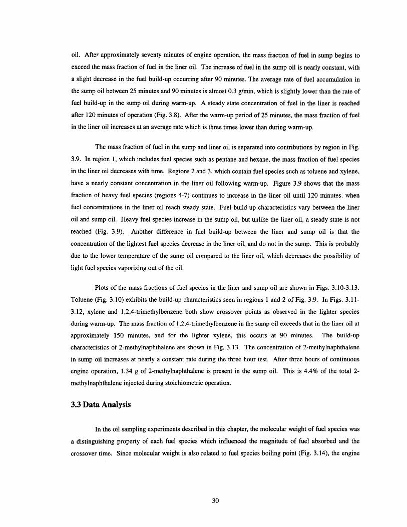
Fig. 3.1 Total fuel mass fraction in liner oil and sump oil during engine warm-up .............................. 36
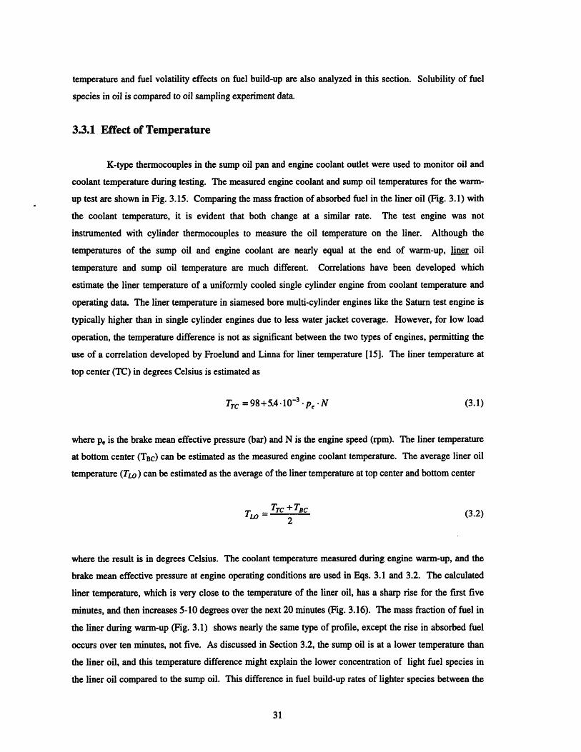
Fig. 3.2 Composition of the mass of fuel in the liner and sump oil during engine warm-up ................ 36
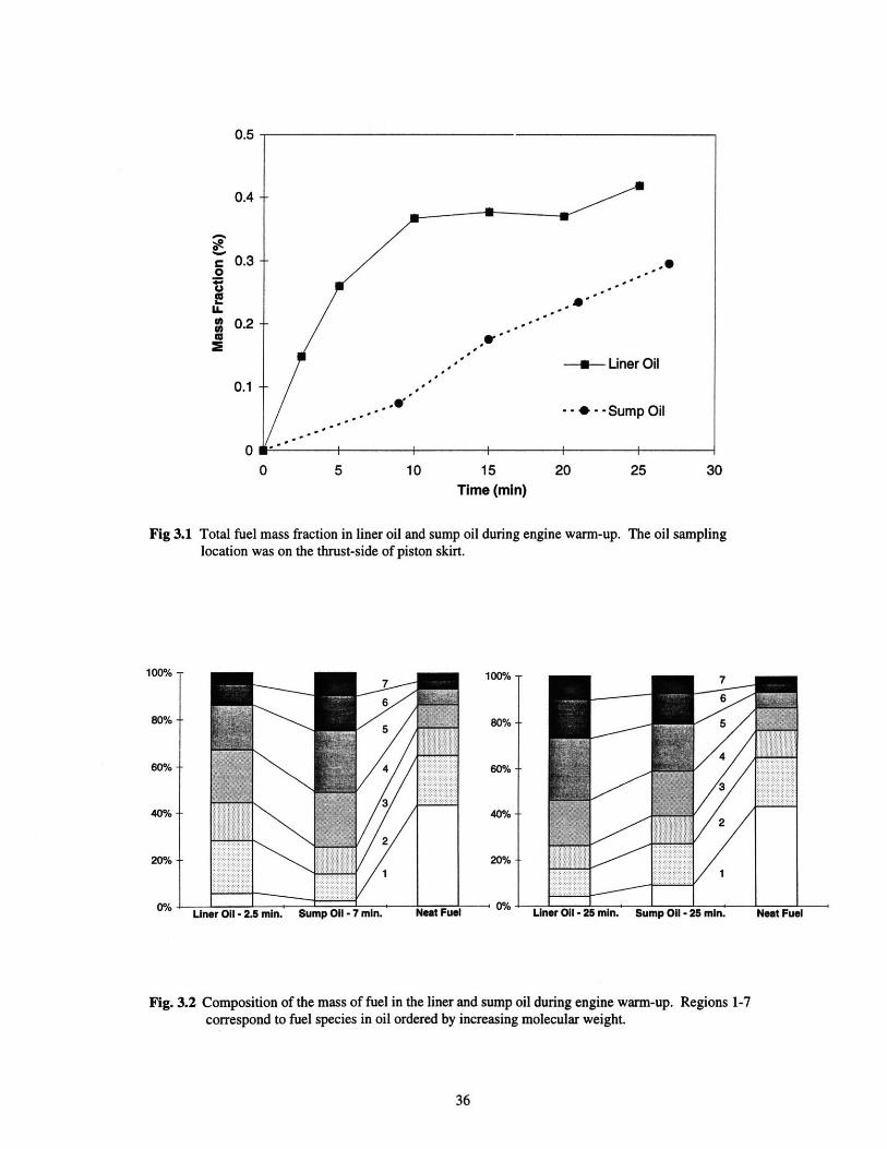
Fig. 3.3 Mass fraction of light fuel species in sump and liner oil during warm-up..............................37
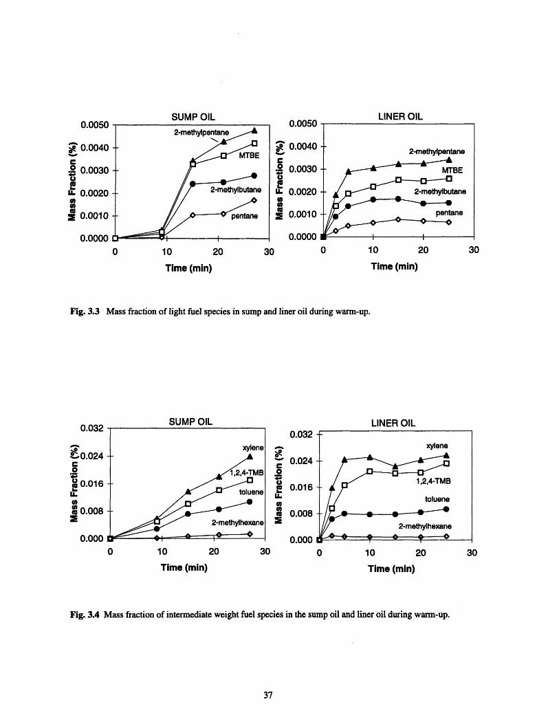
Fig. 3.4 Mass fraction of intermediate weight fuel species in the sump oil and liner ........................... 37
oil during warm-up.
Fig. 3.5 Mass fraction of heavy fuel species in sump and liner oil during warm-up ............................ 38
Fig. 3.6 M ass fraction of toluene in oil..................................................... ........................................ 38
Fig. 3.7 Total fuel mass fraction in liner oil for warm-up oil sampling experiments.......................... 39
Fig. 3.8 Total fuel mass fraction in liner and sump oil for the 3 hour oil sampling experiment ............ 39
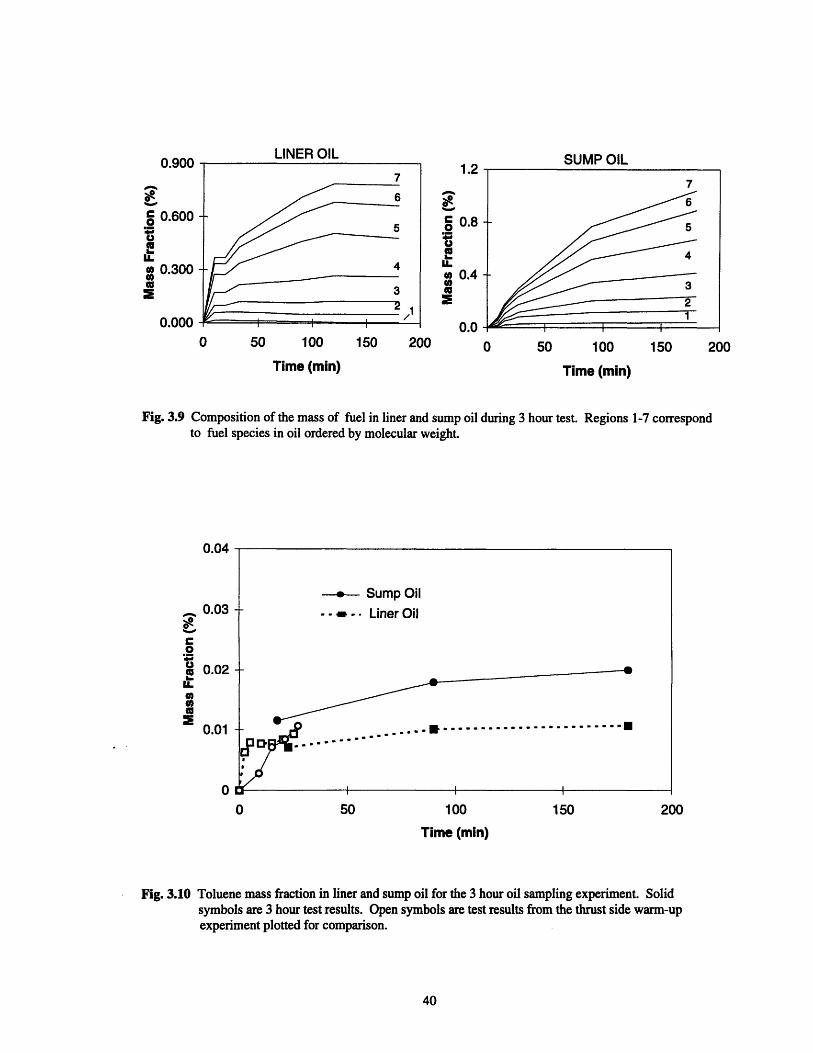
Fig. 3.9 Composition of the mass of fuel in liner and sump oil during 3 hour test...............................40
Fig. 3.10 Toluene mass fraction in liner and sump oil for the 3 hour oil sampling experiment..............40
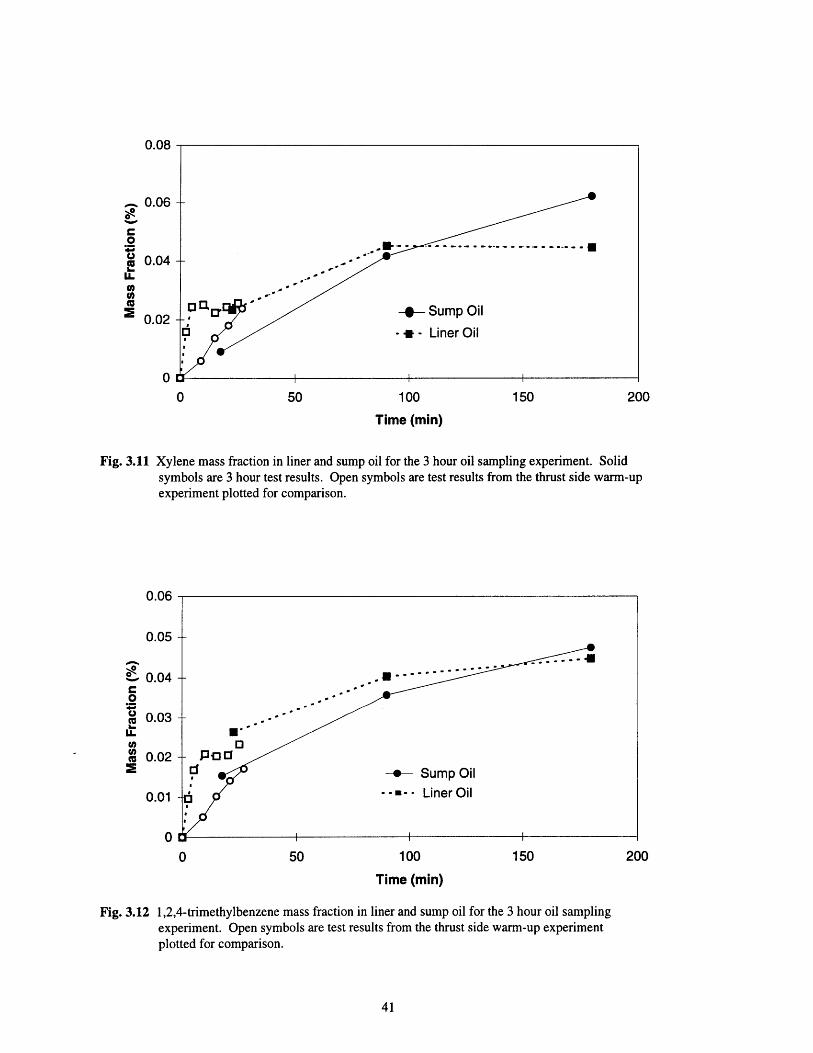
Fig. 3.11 Xylene mass fraction in liner and sump oil for the 3 hour oil sampling experiment .................. 41
Fig. 3.12 1,2,4-trimethylbenzene mass fraction in liner and sump oil for the 3 hour oil sampling............41
experiment.
Fig. 3.13 2-methylnaphthalne mass fraction in liner and sump oil for the 3 hour oil ............................. 42
sampling experiment.
Fig. 3.14 Boiling point vs. molecular weight for some major fuel species in the test gasoline ........... 42
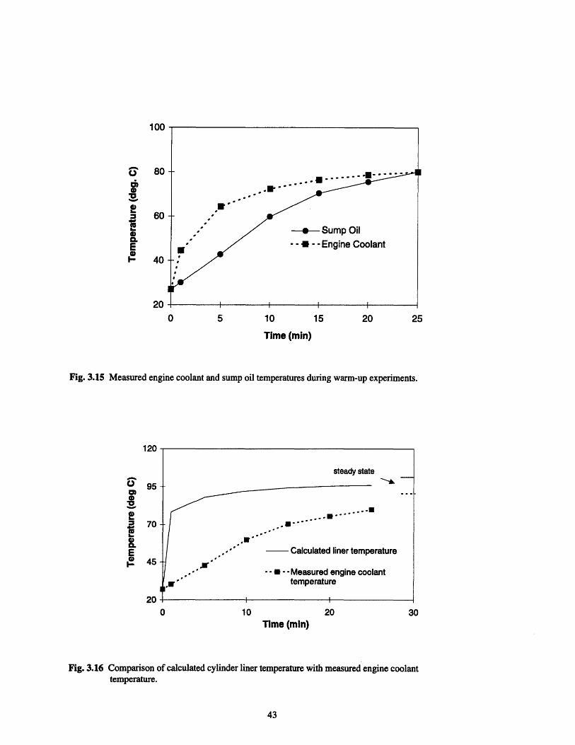
Fig. 3.15 Measured engine coolant and sump oil temperatures during warm-up experiments ............... 43
Fig. 3.16 Comparison of calculated cylinder liner temperature with measured engine coolant..............43temperature.
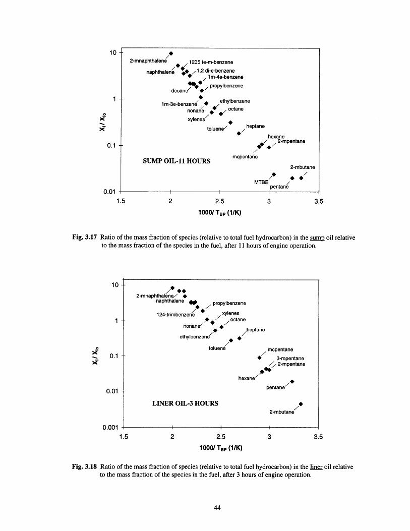
Fig. 3.17 Ratio of the mass fraction of species (relative to total fuel hydrocarbon) .............................. 44in the sumn oil relative to the mass fraction of the species in the fuel,after 11 hours of engine operation.
Fig. 3.18 Ratio of the mass fraction of species (relative to total fuel hydrocarbon) ............................... 44in the liner oil relative to the mass fraction of the species in the fuel,after 3 hours of engine operation.
Fig. 3.19 Comparison of fuel buildup between a paraffinic fuel and................................. ..... 45one blended with 20% aromatic content.
Fig. 4.1 Concentration of crankcase gas HC .................................................................... ................ 50
Fig. 4.2 Composition of crankcase gas at 60 minutes...................................... ........ 50
Fig. 5.1 Framework for fuel transport in engine oil.............................................................66

Fig. 5.2 Simplified fuel transport framework .................................................................... ............... 66
Fig. 5.3 Estimated oil film thickness on the liner for different piston positions ................................... 67
Fig. 5.4 Estimated oil film thickness on piston lands and volume of oil in ring grooves ..................... 67
Fig. 5.5 Sump oil control volume with interacting species fluxes ...................................... .... 68
Fig. 5.6 Calculated results for the oil refreshment rate........................................ ....... 68
Fig. 5.7 Positive crankcase ventilation system in the Saturn 1.9 L engine .............................................. 69
Fig. 5.8 Schematic of experimental setup to measure blow-by gas flow rate .................................... 69
Fig. 5.9 Polynomial curve fits of the mass fraction of fuel species in the liner and sump oil ............... 70
Fig. 5.10 Calculated crankcase gas to sump oil species mass flux thsci ,normalized by ...................... 71
the rate each fuel species is injected into the engine during stoichiometricoperation.
Fig. 5.11 Calculated liner oil fuel species mass flux tneti, normalized by the rate each fuel..................72
species is injected into the engine during stoichiometric operation.
Fig. 5.12 Liner oil control volume with interacting species mass fluxes ....................................... 73
Fig. 5.13 Crankcase gas control volume with interacting species mass fluxes .................................... 73
Fig. 5.14 Curve fit of the crankcase gas mass fractions of toluene and 2-methylpentane .................... 74
Fig. 5.15 Calculated values thLc / hinj, and in•te / rhinji for toluene and 2-methylpentane..................74
Fig. 5.16 Species mass fluxes for light, intermediate, and heavy fuel species at the end of warm-up.......75
Fig. 5.17 Species mass fluxes for light, intermediate, and heavy fuel species after three hours............76
Fig. 5.18 Species mass flux for the total fuel at the end of warm-up and after three hours .................... 77
Fig. 5.19 Example of a calculated species flux with uncertainty bounds ...................................... 77

LIST OF TABLES
Table 2.1 Chevron FR1760 fuel Composition ..................................................................................... 20
Table 5.1 Values for the estimate of fuel fraction in blow-by gas..................................... ..... 56
Table 5.2 Fuel components chosen as modeling inputs....................................... ........ 57
Table 5.3 Uncertainties in model inputs...................................................... ......................................... 63
Table 5.4 Uncertainties in calculated species mass fluxes ...................................................................... 64
Table A .1 Oil Sampling Equipment........................................................... ........................................... 83
Table A.2 Saturn Engine Specifications ........................................................................... .................... 83
Table B.1 Gas flow rates for the Hewlett-Packard Gas Chromatograph..................................................84
Table B.2 Oven temperature program for fuel analysis in oil ........................................ ...... 84
Table B.3 Integration events in Hewlett-Packard Chemstation analysis software ................................... 85
Table B.4 Major fuel species in Chevron FR1760 reference fuel.................................... ..... 85
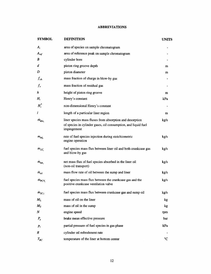
ABBREVIATIONS
SYMBOL DEFINITION UNITS
Ai area of species on sample chromatogram
A,re area of reference peak on sample chromatogram
B cylinder bore
d piston ring groove depth m
D piston diameter m
fch mass fraction of charge in blow-by gas
fr mass fraction of residual gas
h height of piston ring groove m
Hi Henry's constant kPa
Hi non-dimensional Henry's constant
1 length of a particular liner region m
rmabsi liner species mass fluxes from absorption and desorption kg/sof species in cylinder gases, oil consumption, and liquid fuelimpingement
rinji rate of fuel species injection during stoichiometric kg/sengine operation
mLCi fuel species mass flux between liner oil and both crankcase gas kg/sand blow-by gas
rmneti net mass flux of fuel species absorbed in the liner oil kg/s(non-oil transport)
rnoil mass flow rate of oil between the sump and liner kg/s
rhpcv, fuel species mass flux between the crankcase gas and the kg/spositive crankcase ventilation valve
hmsc i fuel species mass flux between crankcase gas and sump oil kg/s
ML mass of oil on the liner kg
Ms mass of oil in the sump kg
N engine speed rpm
Pe brake mean effective pressure bar
Pi partial pressure of fuel species in gas phase kPa
R cylinder oil refreshment rate
TBe temperature of the liner at bottom center °C

SYMBOL DEFINITION UNITS
TLO average temperature of the liner oil °C
TTC temperature of the liner at top center OC
Vi volume of oil in a ring groove m,
xi mole fraction of fuel species in oil
Xi mass fraction of fuel species in oil
Xef mass fraction of a reference standard in GC analysis
X o2 mass fraction of CO2 in burned cylinder gas
xCo2 mass fraction of CO2 in charge
oX Cmass fraction of CO2 in cylinder gas
6 oil film thickness m
e fractional uncertainty
flooded fraction of ring groove volume


CHAPTER 1
INTRODUCTION
1.1 Background
The purpose of reducing hydrocarbon emissions from automotive engines is to avoid the negative
health and atmospheric effects that result when hydrocarbons are released into the atmosphere. Reactive
hydrocarbons and nitric oxides in the troposphere combine in the presence of sunlight to form ozone.
Ozone is a lung and eye irritant and damages crops. Ozone formation in many major cities is a visible result
of unburned hydrocarbons being emitted from internal combustion engines. Hydrocarbons which escape
complete combustion can be hazardous to humans; benzene and 1,3-butadiene are common fuel species
which can be toxic at high levels. Finally, since fuel hydrocarbons are a source of chemical energy, their
emission annually represents thousands of gallons of fuel which have not been productively used.
Engine manufacturers and researchers are addressing the hydrocarbon emission (HC) problem in
internal combustion engines with vigor as a result of increasingly strict global emissions regulations. HC
emissions have been reduced by a factor of three compared to 1972 levels [1]. Much of this reduction came
as a result of the introduction of unleaded fuels. Unleaded fuel allows for closed loop engine control and
effective catalyst exhaust gas after-treatment systems. Engine design measures, such as improvements in
fuel metering, mixture formation, crankcase ventilation, valve timing, ignition systems and combustion
chamber design have also contributed greatly to lowering HC emissions. Cheng et al. outlined a general
framework identifying HC emission sources and their magnitudes [2]. While comprehensive, the
framework only estimates the relative importance of HC sources at warmed-up conditions. Proposed
emission levels of 0.13 g HC/mile in the United States Tier II regulations will require a deeper
understanding of the mechanisms leading to HC emissions [3].
There are several mechanisms by which fuel escapes complete oxidation in the engine. Crevices in
the combustion chamber (spark plug threads, spaces between the piston lands and cylinder wall, head gasket
gaps, valve seat crevices) fill with charge during the intake and compression strokes. This fuel remains
unburned as the flame passes the crevice entrance, and exits to the combustion chamber when the cylinder
pressure decreases. Crevice sources and absorption processes occurring in combustion chamber deposits
and oil layers together may account for 30-60% of the engine-out HC emissions at warmed-up conditions
[4]. Flame quenching is the process by which the flame in the combustion chamber is extinguished near the
cool cylinder walls. This leaves a layer of unburned fuel near the walls which either oxidizes later in the
cycle or is carried into the exhaust port with the burned gases. The amount of quenching varies with
combustion systems but during steady operation is thought to account for 1-5% of engine-out HC emissions
[2]. Engine misfires and incomplete valve closure are other less significant sources of HC emissions.
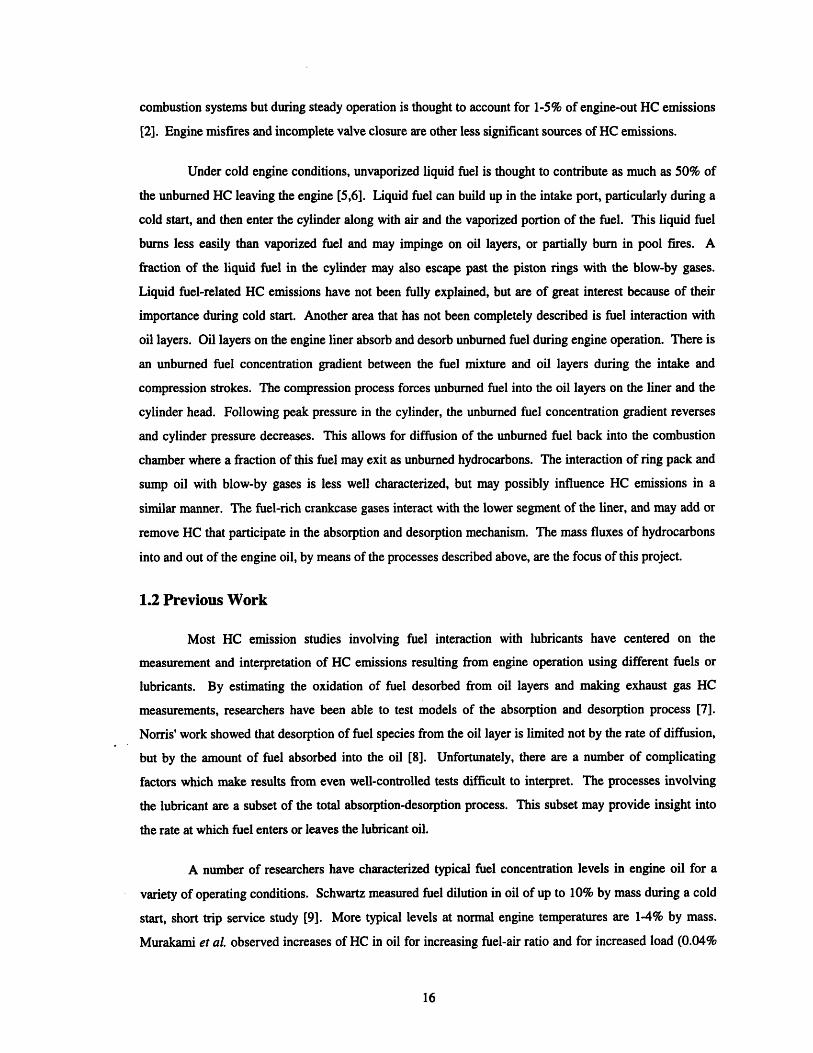
Under cold engine conditions, unvaporized liquid fuel is thought to contribute as much as 50% of
the unburned HC leaving the engine [5,6]. Liquid fuel can build up in the intake port, particularly during a
cold start, and then enter the cylinder along with air and the vaporized portion of the fuel. This liquid fuel
burns less easily than vaporized fuel and may impinge on oil layers, or partially burn in pool fires. A
fraction of the liquid fuel in the cylinder may also escape past the piston rings with the blow-by gases.
Liquid fuel-related HC emissions have not been fully explained, but are of great interest because of their
importance during cold start. Another area that has not been completely described is fuel interaction with
oil layers. Oil layers on the engine liner absorb and desorb unburned fuel during engine operation. There is
an unburned fuel concentration gradient between the fuel mixture and oil layers during the intake and
compression strokes. The compression process forces unburned fuel into the oil layers on the liner and the
cylinder head. Following peak pressure in the cylinder, the unburned fuel concentration gradient reverses
and cylinder pressure decreases. This allows for diffusion of the unburned fuel back into the combustion
chamber where a fraction of this fuel may exit as unburned hydrocarbons. The interaction of ring pack and
sump oil with blow-by gases is less well characterized, but may possibly influence HC emissions in a
similar manner. The fuel-rich crankcase gases interact with the lower segment of the liner, and may add or
remove HC that participate in the absorption and desorption mechanism. The mass fluxes of hydrocarbons
into and out of the engine oil, by means of the processes described above, are the focus of this project.
1.2 Previous Work
Most HC emission studies involving fuel interaction with lubricants have centered on the
measurement and interpretation of HC emissions resulting from engine operation using different fuels or
lubricants. By estimating the oxidation of fuel desorbed from oil layers and making exhaust gas HC
measurements, researchers have been able to test models of the absorption and desorption process [7].
Norris' work showed that desorption of fuel species from the oil layer is limited not by the rate of diffusion,
but by the amount of fuel absorbed into the oil [8]. Unfortunately, there are a number of complicating
factors which make results from even well-controlled tests difficult to interpret. The processes involving
the lubricant are a subset of the total absorption-desorption process. This subset may provide insight into
the rate at which fuel enters or leaves the lubricant oil.
A number of researchers have characterized typical fuel concentration levels in engine oil for a
variety of operating conditions. Schwartz measured fuel dilution in oil of up to 10% by mass during a cold
start, short trip service study [9]. More typical levels at normal engine temperatures are 1-4% by mass.
Murakami et al. observed increases of HC in oil for increasing fuel-air ratio and for increased load (0.04%
HC increase / N-m of torque increase) [10]. Furthermore, decreasing engine temperature resulted in
increased HC emissions. These results support the view that fuel component solubility in oil, which is a
function of temperature and pressure, controls the amount of fuel absorbed in oil. This work attempts to
confirm the role of solubility in the fuel absorption process.
Researchers interested in oil degradation, varnish formation, and HC emissions have sampled and
analyzed engine oil. The method by which oil samples from the engine are obtained is critical to how they
can be used to interpret the processes occurring in different parts of the engine. Samples obtained from the
sump oil alone do not provide a direct view of the processes occurring on the cylinder liner, as there are a
number of opportunities for HC transport to and from the oil, and mixing before it reaches the sump. The
most interesting, and more difficult location from which to sample is on the cylinder liner or in the piston
ring pack. This has typically been accomplished by drilling a sampling hole in the piston and using a
linkage to transport the oil sample out of the engine. Saville et al. used such a mechanism to sample oil
from the liner at sampling rates from 2 to 20 mg/min. [11]. At low sampling rates, changes in oil properties
occurring during warm-up cannot be detected. Murakami et al. sampled a mixture of oil and blow-by from
the piston ring pack and condensed the sample, which may cloud some of the distinction between what HC
are present in the blow-by and what are present in the oil [10]. Our current work aims to sample liner oil at
a sufficiently high rate to give insight into the development of HC concentrations during engine warm-up.
This study is a continuation of work begun by Vincent Frottier of PSA [12]. The gas
chromatographic method he helped develop to analyze fuel content in oil is used and documented here. A
liner oil sampling system was also developed, and is used extensively in this study to provide liner oil
samples. Frottier conducted steady state sump oil sampling which provided baseline data to compare with
liner oil concentrations. A better understanding is needed of the complex processes in which fuel interacts
with the engine oil. Absorption of cylinder gas, crankcase gas and blow-by gas are all processes by which
vaporized fuel can enter the oil. Fuel can leave oil layers through transport between the sump and liner oil,
vaporization, desorption and oil consumption. Liquid fuel interaction with liner oil layers is also possible.
The intent of this work was to capture more fully the basic processes involving the oil, while building on the
knowledge that has been developed.
1.3 Objectives
Previ6us work on HC transport in oil layers consists primarily of tests in which parameters such as
engine conditions, temperatures, fuels and lubricants were varied to determine their effect on hydrocarbon
emissions or fuel concentration in oil. In this work, the liner oil layers, sump oil, blow-by and crankcase

gases were sampled. Subsequent chemical analysis and modeling were undertaken to meet the following
objectives:
1. Develop a framework for fuel-related hydrocarbon transport between the liner oil layers, sump oil,
blow-by and crankcase gases.
2. Determine parameters (both fuel related and operating condition related) controlling the total amount of
fuel transported to the oil.
CHAPTER 2
LINER OIL SAMPLING SYSTEM AND OIL ANALYSIS
A method was developed to obtain liner and sump oil samples from a firing, four-cylinder spark ignition
engine. Upon collection, the samples were analyzed to determine their fuel content, and this information was used to
understand controlling parameters for fuel absorption (Chapter 3) and as input to a fuel transport model (Chapter 5).
There are a number of important considerations for both the hardware and procedure when sampling liner oil. The
oil sampling hardware should not alter normal engine operation. For instance, use of heavy sampling lines or
additional fasteners can change the effective mass of the connecting rod and piston, which may influence engine
performance. The sampling system must be compact, since space available for sampling lines is very limited within
the engine. Finally, the system should be easy to install and maintain, and have a safe failure mode in the high
speeds, temperatures and pressures present in the engine. The procedure for sampling cylinder liner oil is subject to
another set of requirements. The most important of these requirements are liner oil sampling rate and quantity. The
sampling rate must be consistent with periods short enough to capture rapid changes in concentration without
unnecessarily increasing analysis effort. The sampled quantity must be large enough to undergo multiple chemical
analysis tests, yet not so large as to alter the lubrication process in the liner region.
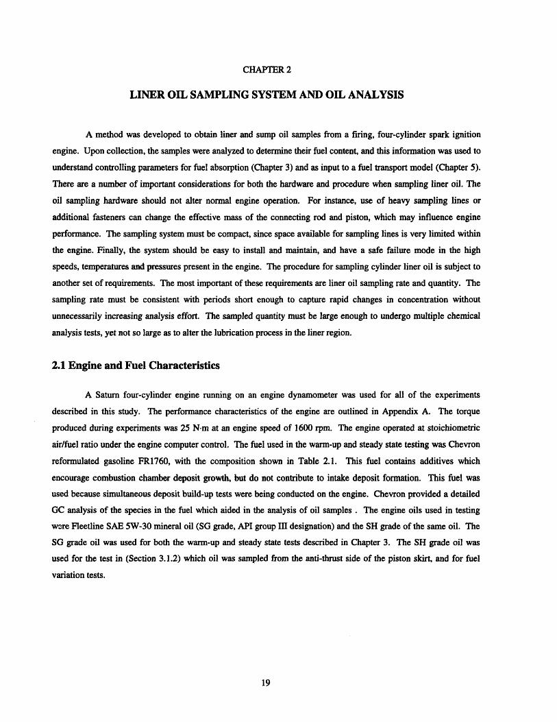
2.1 Engine and Fuel Characteristics
A Saturn four-cylinder engine running on an engine dynamometer was used for all of the experiments
described in this study. The performance characteristics of the engine are outlined in Appendix A. The torque
produced during experiments was 25 N-m at an engine speed of 1600 rpm. The engine operated at stoichiometric
air/fuel ratio under the engine computer control. The fuel used in the warm-up and steady state testing was Chevron
reformulated gasoline FR1760, with the composition shown in Table 2.1. This fuel contains additives which
encourage combustion chamber deposit growth, but do not contribute to intake deposit formation. This fuel was
used because simultaneous deposit build-up tests were being conducted on the engine. Chevron provided a detailed
GC analysis of the species in the fuel which aided in the analysis of oil samples . The engine oils used in testing
were Fleetline SAE 5W-30 mineral oil (SG grade, API group III designation) and the SH grade of the same oil. The
SG grade oil was used for both the warm-up and steady state tests described in Chapter 3. The SH grade oil was
used for the test in (Section 3.1.2) which oil was sampled from the anti-thrust side of the piston skirt, and for fuel
variation tests.

Table 2.1 Chevron FR1760 fuel composition
Chemical Class Percent by Weight
Saturates 49.3
Olefins 9.0
Aromatics 3.15
Oxygenates (MTBE) 10.2 (9.69)
2.2 Liner and Sump Oil Sampling System
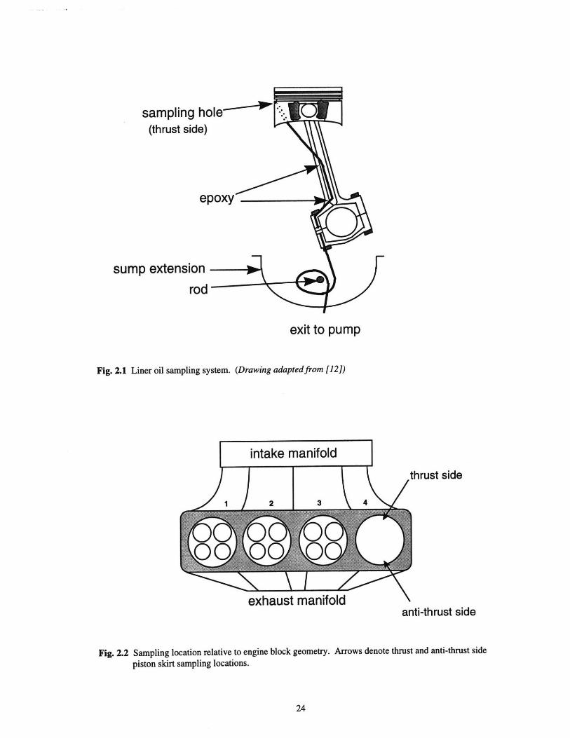
The liner oil sampling system consists of a series of carefully placed sample lines connected to a piston, and
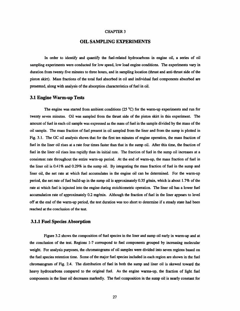
routed along existing engine hardware (Fig. 2.1). A 1 mm diameter hole was drilled through the piston skirt 0.5 mm
below the oil control ring. The hole is located either on the thrust or anti-thrust side of the piston in cylinder 4 of the
engine (Fig. 2.2). A stainless steel (1 mm ID) tube was press-fitted into the hole from the interior of the piston and
then covered with a high temperature epoxy. A flexible, temperature resistant PTFE tube was connected to the
stainless steel, and carefully looped to pick up slack from connecting rod rotation (see Fig. 2.3). This tubing was
positioned in a recessed portion of the connecting rod and passed through a small hole drilled in the shoulder of the
connecting rod bearing cap. The tubing was connected to a strong 0.762 mm ID PEEK tube which was looped
around a rod placed in the sump. This connection was made with a temperature resistant epoxy. The tubing then
exited the sump to a cassette displacement pump, which provided the pressure to set up a sampling flow. Sump oil
was also sampled simultaneously by inserting the 0.762 mm ID tube part way into the oil pan. A description of the
equipment and settings used in liner and sump oil sampling is contained in Appendix A.
A source of difficulty encountered using the sampling hardware was avoiding kinks in the tubing at location
A (Fig. 2.3). This could be seen fairly easily once the piston was installed, by turning the crankshaft over by hand
and observing the tubing in this location. A more serious and frequently occurring problem was breakage of the
connection between the two types of tubing just beyond the bearing cap. This was the result of an incorrect amount
of tubing looped around the rod placed in the sump. A failure of this sort would be detected at the start of oil
sampling and was indicated by a much larger than expected flow of oil from the liner oil sampling line, since the
sampling tubing would be lying within the sump oil. Once correctly installed, the system worked well, permitting
long sampling runs with no failures during operation. As mentioned above, the sampling hole is located on the thrust
side of the piston for some of the experiments and on the anti-thrust side of the piston for others. This location was
chosen based on observations of the lubricant films in an engine with a quartz cylinder which showed that a large
quantity of oil was present between the liner and the piston skirt. Originally, the sampling hole was drilled in
location B (Fig. 2.3), but it was difficult to draw oil from that section of the piston. Attempts to sample oil from this
location resulted in little oil and large amounts of blow-by gas.

2.3 Procedure
The test engine was instrumented to measure oil and coolant temperature, intake manifold average pressure,
exhaust oxygen content and other basic engine parameters. Prior to each experimental run, the engine oil was
flushed and the oil filter was replaced. The engine was motored for approximately ten seconds before starting under
engine computer control. At this time, the cassette pump was activated and continuous sampling of oil from the liner
and sump began. The cassette displacement pump was set at 75% of full output and the flow from the sampling
tubes was regulated with flow restrictors. Restriction of the sump oil sampling flow is necessary since the cassette
pump is set to a high pressure in order to overcome the resistance in the liner oil sampling tube and inertial forces on
oil in the sampling tube. The liner oil sampling tube length is 406 mm, with a corresponding sample transit time of 4
minutes, 16 seconds at the stated cassette pump setting.
After the initial transit time, the oil was deposited into 1.5 ml sample vials which were replaced at short
intervals (3-10 minutes). By adjusting for the sample transit time, it was possible to determine when a particular oil
sample was drawn from the liner. Liner oil was sampled at an average flow rate of between 0.10 - 0.12 ml/min,
which represents removal of 5% of the estimated mass of oil on the cylinder liner in one minute. In Chapter 3, the
percentage of the liner oil mass refreshed each revolution is estimated to be 1.25%. A comparison of these values
shows that it is unlikely that the lubrication of the liner was altered by the sampling method. The liner and piston
were examined after the tests were completed, and no abnormal wear was observed.
2.4 Sample Analysis
Gas chromatography (GC) analysis of the oil samples was used to identify absorbed fuel species and
determine the mass fraction of species in the samples. A number of detector choices are available for this type of GC
analysis. Perhaps the most effective combination of detectors is a flame ionization detector (FID) and a mass
spectrometer (MS). The detectors would have to be used in separate sample runs since each technique destroys the
sample. Sample quantification, cost and complexity make MS difficult, yet it is a very effective technique for
identifying different fuel species. A single FID detector was used in this study because of its availability,
convenience and successful use in related analysis. The strength of the FID is the nearly proportional response of the
detector to the number of carbon atoms in each species sample, making quantification relatively simple. Retention
indices or calibration samples are needed to identify unknown fuel species when using the FID, which is time
consuming but adequate for this work.
Although a number of analysis standards exist for determining the total fuel dilution in oil, one which
provides for the speciation of fuel components in oil was not available. Frottier et al. adapted ASTM method
D3525-93 to allow for speciation of fuel components in engine oil [12]. The selection of an appropriate analytical
column (J&W Scientific DB-1, 60 m length, 0.32 mm inner diameter, 1 pm film thickness) and method allowed for
good separation of fuel species throughout the entire range of absorbed fuel. The same type of column was used in
the Auto/Oil Air Quality Improvement Research Program to separate fuel species in gas emission samples. A pre-
column is used between the inlet and the analytical column to protect the column phase from the heavy oil
components. Sample disturbance from the pre-column was rare, and the analytical column quickly degrades if the
pre-column is not used. An alternate method to preserve the column, which uses flow valves to back-flush the slow
moving heavy oil components from the column was considered, but not used.
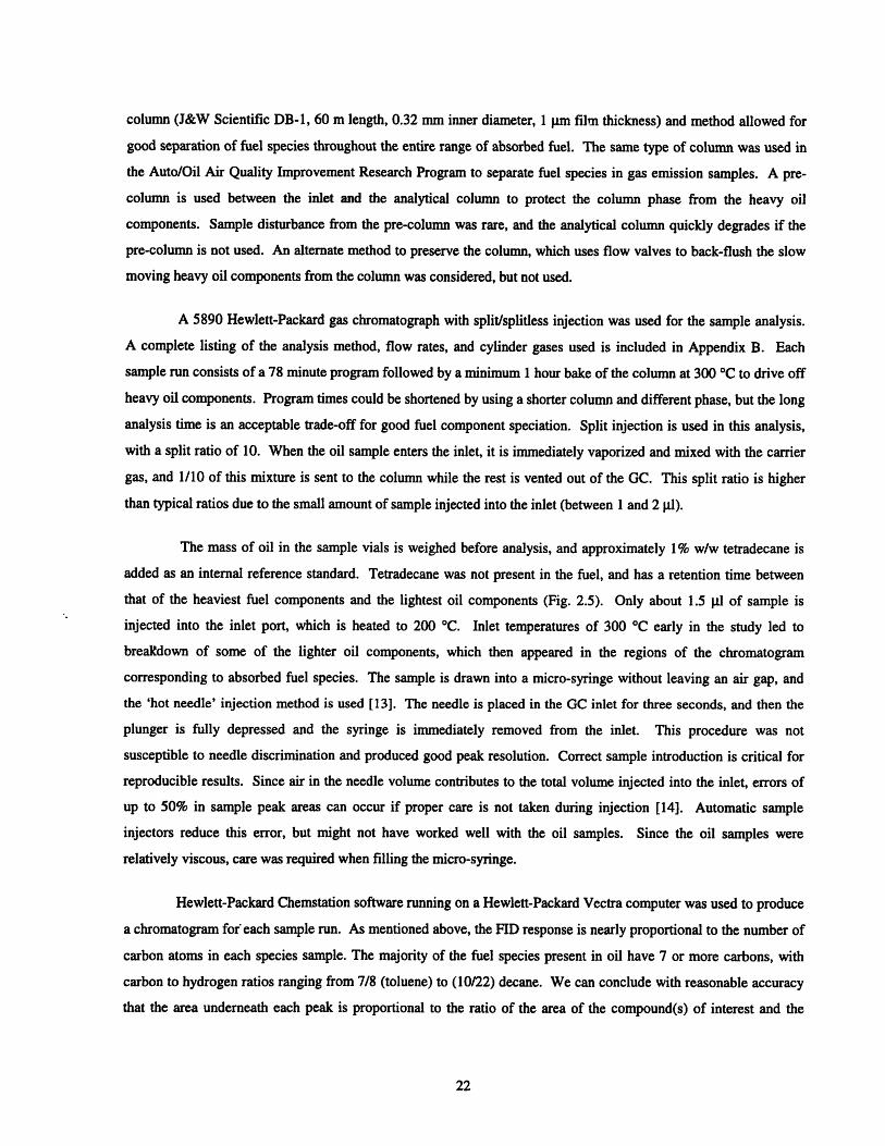
A 5890 Hewlett-Packard gas chromatograph with split/splitless injection was used for the sample analysis.
A complete listing of the analysis method, flow rates, and cylinder gases used is included in Appendix B. Each
sample run consists of a 78 minute program followed by a minimum 1 hour bake of the column at 300 'C to drive off
heavy oil components. Program times could be shortened by using a shorter column and different phase, but the long
analysis time is an acceptable trade-off for good fuel component speciation. Split injection is used in this analysis,
with a split ratio of 10. When the oil sample enters the inlet, it is immediately vaporized and mixed with the carrier
gas, and 1/10 of this mixture is sent to the column while the rest is vented out of the GC. This split ratio is higher
than typical ratios due to the small amount of sample injected into the inlet (between 1 and 2 .l).
The mass of oil in the sample vials is weighed before analysis, and approximately 1% w/w tetradecane is
added as an internal reference standard. Tetradecane was not present in the fuel, and has a retention time between
that of the heaviest fuel components and the lightest oil components (Fig. 2.5). Only about 1.5 .l of sample is
injected into the inlet port, which is heated to 200 OC. Inlet temperatures of 300 °C early in the study led to
breakdown of some of the lighter oil components, which then appeared in the regions of the chromatogram
corresponding to absorbed fuel species. The sample is drawn into a micro-syringe without leaving an air gap, and
the 'hot needle' injection method is used [13]. The needle is placed in the GC inlet for three seconds, and then the
plunger is fully depressed and the syringe is immediately removed from the inlet. This procedure was not
susceptible to needle discrimination and produced good peak resolution. Correct sample introduction is critical for
reproducible results. Since air in the needle volume contributes to the total volume injected into the inlet, errors of
up to 50% in sample peak areas can occur if proper care is not taken during injection [14]. Automatic sample
injectors reduce this error, but might not have worked well with the oil samples. Since the oil samples were
relatively viscous, care was required when filling the micro-syringe.
Hewlett-Packard Chemstation software running on a Hewlett-Packard Vectra computer was used to produce
a chromatogram for each sample run. As mentioned above, the FID response is nearly proportional to the number of
carbon atoms in each species sample. The majority of the fuel species present in oil have 7 or more carbons, with
carbon to hydrogen ratios ranging from 7/8 (toluene) to (10/22) decane. We can conclude with reasonable accuracy
that the area underneath each peak is proportional to the ratio of the area of the compound(s) of interest and the
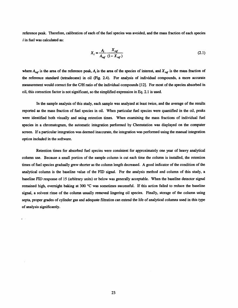
reference peak. Therefore, calibration of each of the fuel species was avoided, and the mass fraction of each species
i in fuel was calculated as:
Xi = A, Xrf (2.1)SAre (1- Xre)
where Aref is the area of the reference peak, A, is the area of the species of interest, and Xref is the mass fraction of
the reference standard (tetradecane) in oil (Fig. 2.4). For analysis of individual compounds, a more accurate
measurement would correct for the C/H ratio of the individual compounds [12]. For most of the species absorbed in
oil, this correction factor is not significant, so the simplified expression in Eq. 2.1 is used.
In the sample analysis of this study, each sample was analyzed at least twice, and the average of the results
reported as the mass fraction of fuel species in oil. When particular fuel species were quantified in the oil, peaks
were identified both visually and using retention times. When examining the mass fractions of individual fuel
species in a chromatogram, the automatic integration performed by Chemstation was displayed on the computer
screen. If a particular integration was deemed inaccurate, the integration was performed using the manual integration
option included in the software.
Retention times for absorbed fuel species were consistent for approximately one year of heavy analytical
column use. Because a small portion of the sample column is cut each time the column is installed, the retention
times of fuel species gradually grew shorter as the column length decreased. A good indicator of the condition of the
analytical column is the baseline value of the FID signal. For the analysis method and column of this study, a
baseline FID response of 15 (arbitrary units) or below was generally acceptable. When the baseline detector signal
remained high, overnight baking at 300 OC was sometimes successful. If this action failed to reduce the baseline
signal, a solvent rinse of the column usually removed lingering oil species. Finally, storage of the column using
septa, proper grades of cylinder gas and adequate filtration can extend the life of analytical columns used in this type
of analysis significantly.
sampling(thrust sid
sump extensiorc
exit to pump
Fig. 2.1 Liner oil sampling system. (Drawing adapted from [12])
intake manifold I
exhaust n a~nifold I
thrust side/
anti-thrust side
Fig. 2.2 Sampling location relative to engine block geometry. Arrows denote thrust and anti-thrust side
piston skirt sampling locations.
·-- ---- I III I
j
I Iui IliB VIta

Fig. 2.3 View of the piston to connecting rod portion of the liner oil sampling system. Location A isthe position where the sampling line would often kink, and B is the location of the originaloil sampling hole.
2 3
toluene|m&p-xylenes
-xylen•
4 i5 6
1,2,4-tdmeth lbenzene
naphtaleneI 1 /
10 20 30 40 50 60 70 80
Retention time (min)
Fig. 2.4 Fuel chromatogram. Reference standard tetradecane visible at 78 minutes.divisions of fuel species by retention time. (Chart adapted from [12])
Regions 1-7 are
A
Wpoxy
1
c-
._0
7 C1(re
I I
2tn- Inrphthajene
. l _ I.
4H30f.)
L.
..-- 1.II .. I- I ----~ - I --- I II I'
-~ w _-i I --unr ~r~ ·- rrcrr~ r~ r~urc-~·llr~vl·mrr~uI--
_l

CHAPTER 3
OIL SAMPLING EXPERIMENTS
In order to identify and quantify the fuel-related hydrocarbons in engine oil, a series of oil
sampling experiments were conducted for low speed, low load engine conditions. The experiments vary in
duration from twenty five minutes to three hours, and in sampling location (thrust and anti-thrust side of the
piston skirt). Mass fractions of the total fuel absorbed in oil and individual fuel components absorbed are
presented, along with analysis of the absorption characteristics of fuel in oil.
3.1 Engine Warm-up Tests
The engine was started from ambient conditions (25 OC) for the warm-up experiments and run for
twenty seven minutes. Oil was sampled from the thrust side of the piston skirt in this experiment. The
amount of fuel in each oil sample was expressed as the mass of fuel in the sample divided by the mass of the
oil sample. The mass fraction of fuel present in oil sampled from the liner and from the sump is plotted in
Fig. 3.1. The GC oil analysis shows that for the first ten minutes of engine operation, the mass fraction of
fuel in the liner oil rises at a rate four times faster than that in the sump oil. After this time, the fraction of
fuel in the liner oil rises less rapidly than its initial rate. The fraction of fuel in the sump oil increases at a
consistent rate throughout the entire warm-up period. At the end of warm-up, the mass fraction of fuel in
the liner oil is 0.41% and 0.29% in the sump oil. By integrating the mass fraction of fuel in the sump and
liner oil, the net rate at which fuel accumulates in the engine oil can be determined. For the warm-up
period, the net rate of fuel build-up in the sump oil is approximately 0.35 g/min, which is about 1.7% of the
rate at which fuel is injected into the engine during stoichiometric operation. The liner oil has a lower fuel
accumulation rate of approximately 0.2 mg/min. Although the fraction of fuel in the liner appears to level
off at the end of the warm-up period, the test duration was too short to determine if a steady state had been
reached at the conclusion of the test.
3.1.1 Fuel Species Absorption
Figure 3.2 shows the composition of fuel species in the liner and sump oil early in warm-up and at
the conclusion of the test. Regions 1-7 correspond to fuel components grouped by increasing molecular
weight. For analysis purposes, the chromatograms of oil samples were divided into seven regions based on
the fuel species retention time. Some of the major fuel species included in each region are shown in the fuel
chromatogram of Fig. 2.4. The distribution of fuel in both the sump and liner oil is skewed toward the
heavy hydrocarbons compared to the original fuel. As the engine warms-up, the fraction of light fuel
components in the liner oil decreases markedly. The fuel composition in the sump oil is nearly constant for
all regions except regions 1 and 2, which contain the lightest fuel components. Figure 3.3 shows that while
the total fuel concentration in the liner and sump oil increases, the concentration of the major light fuel
species (pentane, 2-methylbutane, Methyl Tertiary Butyl Ether (MTBE), and 2-methylhexane) does not
increase from initial levels. In fact, at 27 minutes, these components have nearly reached a steady state
concentration.
Some of the intermediate weight fuel species (7-9 carbon atoms) in the liner and sump oil are
plotted in Fig. 3.4. Similarities in the build-up rate observed for light species are present for 2-
methylhexane, toluene, xylene and 1,2,4-trimethylbenzene. One difference is that mass fractions of most of
the intermediate weight fuel species in the liner and sump oil are 5 to 8 times as large as that of the lighter
fuel species at the end of warm-up. A comparison of the relative amounts of these species in the fuel
(Appendix B) indicates that this difference in build-up does not scale with the relative amount of each
species in the fuel. Also, unlike the sump oil concentrations of the lighter fuel species, the intermediate
weight fuel species are increasing steadily in the sump oil. The intermediate weight fuel species
concentrations in the liner oil appear to be at a steady state after 27 minutes. The mass fraction in oil of two
heavy fuel species (10-11 carbons) is shown in Fig. 3.5. Both heavy species have similar sump and liner oil
concentrations throughout warm-up. During warm-up, the average rate of 2-methylnaphthalene and
naphthalene build-up in the liner oil is nearly twice as fast as in the sump. The consistent increase of these
heavy species in the liner oil differs from the rate of increase of the lighter species.
In Fig. 3.6, the liner and sump oil mass fractions of toluene are plotted together. After
approximately 20 minutes, the mass fraction of toluene in the sump oil begins to exceed the fraction of
toluene in the liner oil. The fact that the sump oil species concentration can exceed the liner oil species
concentration indicates that there is another source of the particular species to the sump oil. However, it is
also possible that fuel is quickly desorbing from the liner after being splashed up from the sump. In Fig.
3.3, the mass fractions of 2-methylpentane and MTBE in the liner oil also overtake the sump mass fractions
early in warm-up. The time necessary for more fuel to accumulate in the sump than in the liner oil is related
to molecular weight. Heavier fuel species such as the 2-methylnaphthalene, naphthalene and 1,2,4-
trimethylbenzene are present in higher fractions in the liner oil than in the sump oil during warm-up (Figs.
3.4-3.5).
3.1.2 Anti-thrust Side Sampling Location
In order to determine how fuel concentration varies along the circumference of the liner oil, a
warm-up experiment was conducted in which oil was drawn from the anti-thrust side of the piston skirt.
The operating conditions and fuel were the same as for the thrust side warm-up test, except that the SH
grade of engine oil was used in the anti-thrust side test. As shown in Fig. 2.2, the sampling location in this
test is on the exhaust side of the piston skirt, directly opposite of the intake-side location of the previous
test. Depending on the injector spray characteristics and cylinder air motion, the amount of liquid fuel
which impinges on the exhaust side of the cylinder may be different than on the intake side. This specific
sampling location was chosen because it was likely that there would be sufficient oil to sample, and because
the location of the sampling line did not have to be altered on the connecting rod. The only modification to
the liner oil sampling system was a new piston with a hole drilled in the appropriate location.
Fig 3.7 shows a comparison between the fuel mass fraction in the liner oil during warm-up for both
sampling locations. For the first 5-7 minutes of engine operation the mass fraction of fuel in the liner oil is
identical for both locations. From 10 minutes until the conclusion of the test, the oil sampled from the anti-
thrust side of the piston skirt had approximately 20% less absorbed fuel than the thrust side. Likewise, the
fuel mass fraction in the sump oil during the anti-thrust test was approximately 25% less than in the thrust-
side test. It is uncertain why the sump and liner oil concentrations in this particular test were lower, since
engine temperatures were nearly identical to the previous warm-up test. One possibility for the difference
in fuel absorbed is the slight difference in oils used in each test. Regardless of the difference in oil
specification, relative to the sump oil fuel concentration, the concentration of fuel in the liner oil for both
sampling locations is nearly identical. Analysis of the oil samples from the anti-thrust test showed that the
composition of fuel species in both sampling locations was also very similar.
3.2 Three Hour Oil Sampling
There were several objectives to conducting a longer duration oil sampling test. One objective was
to determine the liner and sump oil fuel species concentrations as they approached steady state. It was also
of interest to determine if the crossover points discussed in Section 3.1 occur for all fuel species. Finally,
concentration data from longer test runs show how fuel is absorbed and transported within the oil at
constant temperature. The conditions and parameters of the three-hour oil sampling test were identical to
the thrust side warm-up test in Section 3.1, except the engine operated for a longer, three hour time interval.
During this test, oil was sampled from the thrust side of the piston skirt, as in Section 3.1.1. The final
coolant and oil temperatures for the three hour test were 89 °C, which is 9 *C higher than at the end of
warm-up. The temperature profiles for both tests were identical for the warm-up period, with the 9 'C
increase in temperature occurring over 155 minutes. The effect of oil and coolant temperatures on fuel
build-up is discussed in Section 3.3.
The mass fraction of fuel in the liner and sump oil for the three hour test is plotted in Fig. 3.8. In
this test, the fuel mass fraction in the sump oil after three hours is 1.04%, compared to 0.78% in the liner
oil. After approximately seventy minutes of engine operation, the mass fraction of fuel in sump begins to
exceed the mass fraction of fuel in the liner oil. The increase of fuel in the sump oil is nearly constant, with
a slight decrease in the fuel build-up occurring after 90 minutes. The average rate of fuel accumulation in
the sump oil between 25 minutes and 90 minutes is almost 0.3 g/min, which is slightly lower than the rate of
fuel build-up in the sump oil during warm-up. A steady state concentration of fuel in the liner is reached
after 120 minutes of operation (Fig. 3.8). After the warm-up period of 25 minutes, the mass fraction of fuel
in the liner oil increases at an average rate which is three times lower than during warm-up.
The mass fraction of fuel in the sump and liner oil is separated into contributions by region in Fig.
3.9. In region 1, which includes fuel species such as pentane and hexane, the mass fraction of fuel species
in the liner oil decreases with time. Regions 2 and 3, which contain fuel species such as toluene and xylene,
have a nearly constant concentration in the liner oil following warm-up. Figure 3.9 shows that the mass
fraction of heavy fuel species (regions 4-7) continues to increase in the liner oil until 120 minutes, when
fuel concentrations in the liner oil reach steady state. Fuel-build up characteristics vary between the liner
oil and sump oil. Heavy fuel species increase in the sump oil, but unlike the liner oil, a steady state is not
reached (Fig. 3.9). Another difference in fuel build-up between the liner and sump oil is that the
concentration of the lightest fuel species decrease in the liner oil, and do not in the sump. This is probably
due to the lower temperature of the sump oil compared to the liner oil, which decreases the possibility of
light fuel species vaporizing out of the oil.
Plots of the mass fractions of fuel species in the liner and sump oil are shown in Figs. 3.10-3.13.
Toluene (Fig. 3.10) exhibits the build-up characteristics seen in regions 1 and 2 of Fig. 3.9. In Figs. 3.11-
3.12, xylene and 1,2,4-trimethylbenzene both show crossover points as observed in the lighter species
during warm-up. The mass fraction of 1,2,4-trimethylbenzene in the sump oil exceeds that in the liner oil at
approximately 150 minutes, and for the lighter xylene, this occurs at 90 minutes. The build-up
characteristics of 2-methylnaphthalene are shown in Fig. 3.13. The concentration of 2-methylnaphthalene
in sump oil increases at nearly a constant rate during the three hour test. After three hours of continuous
engine operation, 1.34 g of 2-methylnaphthalene is present in the sump oil. This is 4.4% of the total 2-
methylnaphthalene injected during stoichiometric operation.
3.3 Data Analysis
In the oil sampling experiments described in this chapter, the molecular weight of fuel species was
a distinguishing property of each fuel species which influenced the magnitude of fuel absorbed and the
crossover time. Since molecular weight is also related to fuel species boiling point (Fig. 3.14), the engine
temperature and fuel volatility effects on fuel build-up are also analyzed in this section. Solubility of fuel
species in oil is compared to oil sampling experiment data.
3.3.1 Effect of Temperature
K-type thermocouples in the sump oil pan and engine coolant outlet were used to monitor oil and
coolant temperature during testing. The measured engine coolant and sump oil temperatures for the warm-
up test are shown in Fig. 3.15. Comparing the mass fraction of absorbed fuel in the liner oil (Fig. 3.1) with
the coolant temperature, it is evident that both change at a similar rate. The test engine was not
instrumented with cylinder thermocouples to measure the oil temperature on the liner. Although the
temperatures of the sump oil and engine coolant are nearly equal at the end of warm-up, liner oil
temperature and sump oil temperature are much different. Correlations have been developed which
estimate the liner temperature of a uniformly cooled single cylinder engine from coolant temperature and
operating data. The liner temperature in siamesed bore multi-cylinder engines like the Saturn test engine is
typically higher than in single cylinder engines due to less water jacket coverage. However, for low load
operation, the temperature difference is not as significant between the two types of engines, permitting the
use of a correlation developed by Froelund and Linna for liner temperature [15]. The liner temperature at
top center (TC) in degrees Celsius is estimated as
Tc = 98+5.4-10-3 -p, -N (3.1)
where Pc is the brake mean effective pressure (bar) and N is the engine speed (rpm). The liner temperature
at bottom center (TBc) can be estimated as the measured engine coolant temperature. The average liner oil
temperature (TLo) can be estimated as the average of the liner temperature at top center and bottom center
Trc + TBcTLO = (3.2)
2
where the result is in degrees Celsius. The coolant temperature measured during engine warm-up, and the
brake mean effective pressure at engine operating conditions are used in Eqs. 3.1 and 3.2. The calculated
liner temperature, which is very close to the temperature of the liner oil, has a sharp rise for the first five
minutes, and then increases 5-10 degrees over the next 20 minutes (Fig. 3.16). The mass fraction of fuel in
the liner during warm-up (Fig. 3.1) shows nearly the same type of profile, except the rise in absorbed fuel
occurs over ten minutes, not five. As discussed in Section 3.2, the sump oil is at a lower temperature than
the liner oil, and this temperature difference might explain the lower concentration of light fuel species in
the liner oil compared to the sump oil. This difference in fuel build-up rates of lighter species between the

sump and liner oil is seen in Fig. 3.2, where the light fuel species are a larger fraction of the fuel in the sump
oil. The temperature difference between the sump and liner oil is as high as 50 OC during the first minute of
warm-up, and falls to approximately 10 'C at steady state. This temperature difference might lead to less
vaporization of the sump fuel species, or affect the temperature dependent solubility process.
3.3.2 Solubility
The characteristics of fuel solubility in oil are examined in this section. The solubility of fuel in oil
is often described by an equation of the form:
Pi = Hi Yi (3.3)
where pi is the partial pressure of the fuel species in the gas phase, Yi is the mole fraction of the fuel species
in the oil, and Hi is the Henry's constant of the particular species. Hi is a temperature dependent inverse
solubility parameter which is determined by experiment. Equation 3.3 is only valid for small concentrations
of fuel in the oil, which holds for the concentrations measured in this study. An alternate form of Eq. 3.3 is
obtained by multiplying H by the ratio of the oil and fuel molecular weights. The resulting solubility
parameter is H*, which has units of pressure. The controlling law for solubility becomes
p, = Hi * X, (3.4)
where Xi is the mass fraction of fuel in oil. If Eq. 3.4 holds, engine oil at different temperatures will absorb
different amounts of fuel, since Hi is temperature dependent. The oil in the liner and sump is exposed to
different thermal conditions which results in a temperature difference of 20 degrees between the warmer
liner oil and the sump oil at the end of engine warm-up (Fig. 3.16). Using the concentration measurements
made in the crankcase gas and in the sump oil (Chapter 4), the partial pressure of several fuel species in the
gas phase was compared to the corresponding concentration of fuel in the sump oil for up to 60 minutes,
using Eq. 3.4. The results from the calculations showed that the measured concentrations of fuel species in
the crankcase gas were substantially lower (10%-50%) than the equilibrium concentrations predicted by Eq.
3.4. Since there may have been sampling losses of the crankcase gas, it was difficult to draw firm
conclusions from those calculations.

3.3.3 Fuel Species Boiling Point
In this section, measurements of fuel absorbed in the sump oil of the Saturn engine are analyzed.
During these tests, the mass fraction of fuel in the sump oil reached a steady state of 1.35% after fifteen
hours. The fuel and oil used in this steady-state experiment are identical to those used in the thrust-side
warm-up tests of Section 3.1. The engine operating conditions were slightly different than in the tests
described previously. An alternating cycle was used where the engine operated for 6 minutes at 1400
rpm/16.5 N-m, and 6 minutes at 2200 rpm/49.5 N.m. The purpose of this analysis is to compare the steady
state species concentrations in the sump oil with steady state concentrations in the liner oil from the three
hour test.
In order to determine the effect of temperature on fuel build-up in oil, the mass fraction of fuel
species in the sump oil at 11 hours was compared to fuel species boiling points. In Fig. 3.17, the vertical
axis is the ratio of the mass fraction of species (relative to total fuel hydrocarbon) in the sump oil relative to
the mass fraction of the species in the fuel. The horizontal axis is the reciprocal boiling point of each
species multiplied by 1000. There is a strong correlation between the mass fraction of fuel species in the
sump oil and the individual boiling points. This correlation indicates that for increasing fuel species
volatility, there is a decreasing amount of the fuel species absorbed in the oil. The mass fractions of fuel
species in the liner oil can be plotted in the same manner. In Fig. 3.18, fuel species are plotted using mass
fractions in liner oil from the three hour sampling experiment of Section 3.2. The same relationship of
increased fuel absorption for species with high boiling points is observed. A line drawn though the points
on both plots indicates similar slopes for both liner and sump data. The slope of the sump oil data in the
semi-log plot (Fig. 3.17) is -2200 K and is -2400 K for the liner data in Fig. 3.18.
3.3.4 Fuel Variation Tests
The purpose of varying fuels was to distinguish between the effects of solubility and fuel volatility
on fuel build-up in oil. Even though GC analysis allows for speciation of the Chevron fuel used in previous
tests, distinct fuels can provide data which isolates specific species properties. Two specially blended
research fuels provided by Exxon were used in warm-up tests in which oil was only sampled from the sump.
One of the fuels tested was a fully-blended paraffinic fuel, and the other was a paraffinic fuel with 20%
aromatic content. The Reid vapor pressure of the fuels was similar, as were the distillation curves. Because
the fuels had comparable volatility, the presence of a significant fraction of aromatics in one fuel makes the
solubility of fuel species in oil a differentiating factor. Generally, the solubility of aromatic fuel species in
oil is higher than for paraffins.

The engine operating conditions in the fuel variation tests were identical to the warm-up test in
Section 3.1. The lubricant used in these experiments was SAE 5W-30 mineral oil with the SH designation.
As shown in Fig. 3.19, a higher mass fraction of the paraffinic-aromatic fuel was present in the sump oil
during warm-up than the fully-blended paraffinic fuel. Gas chromatography analysis provided by Exxon of
two oil samples at the end of warm-up also confirmed this result. The increased buildup of the more soluble
fuel indicates that the effect of volatility in Section 3.3.3 may be separate from the influence of solubility in
fuel build-up. If individual species of comparable volatility were identified with different solubility in oil,
the measured mass fractions would clarify the role of solubility in fuel build-up. While the integrated
results of the fuel variation tests suggest that solubility has a distinct effect from fuel volatility, it was not
possible to identify fuel species in the test fuels which matched the above criteria. A complete analysis of
the individual fuel species in both fuels was not available, so a detailed analysis of the absorption
characteristics was not possible at this time.
3.4 Conclusions
In this chapter the accumulation of fuel species in the liner and sump oil of a four cylinder, spark-
ignition engine was described for low load, low speed conditions. The engine was operated using a
standard fuel of known composition and a commercial mineral oil. During the first ten minutes of warm-up,
the mass fraction of fuel in the liner oil rises at a rate nearly four times faster than in the sump oil, with a
build-up rate that matches the change in liner oil temperature. At the end of warm-up, the mass fraction of
fuel in the liner oil is 0.41%, and 0.29% in the sump oil. For the warm-up period, the net rate of fuel build-
up in the sump oil is about 1.7% of the rate at which fuel is injected into the engine during stoichiometric
operation. After three hours of engine operation, the fuel mass fraction in the sump oil is 1.04%, compared
to 0.78% in the liner oil. In this study, the point where the total fuel concentration in the sump oil exceeds
the fuel concentration in the liner oil occurs at approximately 70 minutes of engine operation. This
crossover point indicates that there is another source of fuel to the sump oil.
The distribution of fuel species in oil is skewed toward the heavy hydrocarbons, and the difference
in absorption does not scale with the relative amount of each species in the fuel. Light fuel species reach
the concentration crossover point between the liner and sump oil within the engine warm-up period, and
also reach steady state during this time. Intermediate weight fuel species in the liner oil reach a steady state
concentration within 100 minutes of operation and approach a steady state in the sump oil by the end of the
three hour experiment. Heavy fuel species in the oil reach a steady state in the liner oil after 120 minutes
but are still increasing in the sump after three hours. For the heaviest fuel species, up to 4.5% of the total
amount injected is present in the sump oil after three hours. Relative to the sump oil fuel concentration, the
concentration of fuel in liner oil on the thrust and anti-thrust sides of the piston skirt is nearly identical.

There is a strong correlation between the mass fraction of fuel species absorbed and individual
boiling points, in both the liner and sump oil at steady state. The relationship between species absorption
and boiling point was nearly identical in both the sump oil and the liner oil. This correlation indicates that
for increasing fuel species volatility, there is a decreasing amount of the fuel species absorbed in engine oil.
In a test with specially blended fuels of similar volatility, the sump oil mass fraction of the higher solubility
fuel was approximately 25% greater than the sump oil mass fraction of the lower solubility fuel.
0.3
0.2
0.1
05 10 15 20 25
Time (min)
Fig 3.1 Total fuel mass fraction in liner oil and sump oil during engine warm-up.location was on the thrust-side of piston skirt.
l lK./o-
80%-
60% -
40% -
20% -
0%-
00o%
80%
60%
400
20%
I I -Liner OI -2.5 min. S5
The oil sampling
Fig. 3.2 Composition of the mass of fuel in the liner and sump oil during engine warm-up. Regions 1-7correspond to fuel species in oil ordered by increasing molecular weight.
I - -~ . -~P
'^^,'-
----
SUMP OIL 0005 N/t•~
0 10 20
V.VV•J
S0.0040
g 0.0030
U, 0.0020
I 0.0010
0.00000 10 20
Time (min) Time (min)
Fig. 3.3 Mass fraction of light fuel species in sump and liner oil during warm-up.
0.032
0.024
0.016
0.008
0.0000 10 20
Time (min)
LINER OIL
0 10 20
Time (min)
Fig. 3.4 Mass fraction of intermediate weight fuel species in the sump oil and liner oil during warm-up.
0.0050
S0.0040
.0 0.0030
0.0020
2 0.0010
0.0000
0.032
0•.024
o0.016
0 0.008
0.000
LINER OIL

A AAn
OR 0.0120
g 0.008uL.
3 0.004
0
0
SUMP OILA A1
.2
S0.008u.
0S0.004 -U.
10 20 30
Time (min)
LINER OIL
Time (min)
Fig. 3.5 Mass fraction of heavy fuel species in sump and liner oil during warm-up.
0.012
0 0.0080
IL
W 0.004
00 10 20
Time (min)
Fig. 3.6 Mass fraction of toluene in oil. Crossover point where sump oil toluene mass fractionexceeds mass fraction of toluene in liner oil occurs at 20 minutes.
2-methylnaphthalene
naphthalene
2-methylnaphthalene
naphthalene
I ·.
-
I
" I II • " " II

0.6
0.5
0.4
m 0.3LLU-
0 0.2
0.1
0
10 20
Time (min)
Fig. 3.7 Total fuel mass fraction in liner oil for warm-up oil sampling experiments. Oil samplinglocations are from the thrust and anti-thrust side of the piston skirt.
1.2
1
•-01 0.8
0.6u.
0.4
0.2
00 50 100 150 200
Time (min)
Fig. 3.8 Total fuel mass fraction in liner and sump oil for the 3 hour oil sampling experiment. Solidsymbols are 3 hour test results. Open symbols are test results from the thrust side warm-upexperiment plotted for comparison.
LINER OIL SUMP OIL
0 50 100 150 200
Time (min)
1.2
c 0.8
'.
0.4
0.00 50 100 150 200
Time (min)
Fig. 3.9 Composition of the mass of fuel in liner and sump oil during 3 hour test. Regionsto fuel species in oil ordered by molecular weight.
0.04
0.03
0.02
0.01
0 50 100 150
Time (min)
1-7 correspond
200
Fig. 3.10 Toluene mass fraction in liner and sump oil for the 3 hour oil sampling experiment. Solidsymbols are 3 hour test results. Open symbols are test results from the thrust side warm-upexperiment plotted for comparison.
0.900
0.600
IL
* 0.300
0.000
0.08
0.06
0.04
0.02
0 50 100 150 200
Time (min)
Fig. 3.11 Xylene mass fraction in liner and sump oil for the 3 hour oil sampling experiment. Solidsymbols are 3 hour test results. Open symbols are test results from the thrust side warm-upexperiment plotted for comparison.
0.06
0.05
0.04
0.03
o 0.02
0.01
0 50 100 150
Time (min)
Fig. 3.12 1,2,4-trimethylbenzene mass fraction in liner and sump oil for the 3 hour oil samplingexperiment. Open symbols are test results from the thrust side warm-up experimentplotted for comparison.
200

0.08
0.06
0.04
0.02
50 100 150 200
Time (min)
Fig. 3.13 2-methylnaphthalne mass fraction in liner and sump oil for the 3 hour oil sampling experiment.Solid symbols are 3 hour test results. Open symbols are test results from the thrust side warm-up experiment plotted for comparison.
550
%9 450
0
o 350m
25070 100 130 160 190
Molecular Weight (g/mol)
Fig. 3.14 Boiling point vs. molecular weight for some major fuel species in the test gasoline. Points whichstack vertically are aromatic compounds in which the benzene ring has the same number ofsubstituents.
100
200 5 10 15 20 2
Time (min)
Fig. 3.15 Measured engine coolant and sump oil temperatures during warm-up experiments.
120
0 10 20 30Time (min)
Fig. 3.16 Comparison of calculated cylinder liner temperature with measured engine coolanttemperature.
5
10 -
1-
0.1 -
0.012.5
1000/ Tap (1/K)
Fig. 3.17 Ratio of the mass fraction of species (relative to total fuel hydrocarbon) in the sump oil relativeto the mass fraction of the species in the fuel, after 11 hours of engine operation.
0.01
J.VJ I
2.5
1000/ TBP (1/K)
3.5
Fig. 3.18 Ratio of the mass fraction of species (relative to total fuel hydrocarbon) in the liner oil relativeto the mass fraction of the species in the fuel, after 3 hours of engine operation.
2-mnaphthalene 1235 te-m-benzene
naphthalene 1,2 di-e-benzene1 m-4e-benzene
decane"/k / propylbenzene
1m-3e-benzen ethylbenzenenonane octane
xylenes"
toluene/ heptanehexane
/ 2-mpentane
SUMP OIL-11 HOURS mcpentane2-mbutane
MTBE /pentaneI II
2-mnaphthalene/ *naphthalene • propylbenzene
124-trmbenzene xylenes* Z' zoctane
nonane /oct heptaneethylbenzene /heptane
toluene mcpentane
3-mpentane7 2-mpentane
hexane
pentane
LINER OIL-3 HOURS2-mbutane
I I I II I I
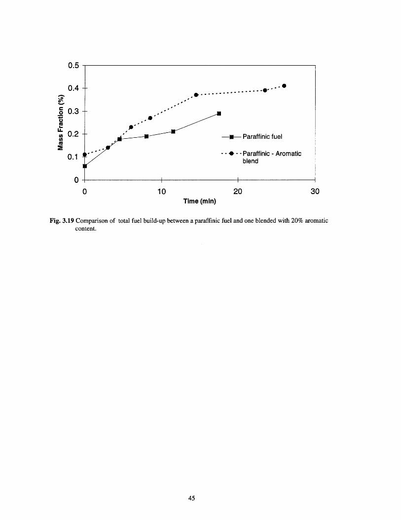
U.3
0.4
o 0.3
U. 0.2
0.1
00 10 20 30
Time (min)
Fig. 3.19 Comparison of total fuel build-up between a paraffinic fuel and one blended with 20% aromaticcontent.


CHAPTER 4
CRANKCASE GAS SAMPLING EXPERIMENTS
The crankcase gas contains fuel species from a number of sources. The processes which might
contribute fuel to the crankcase are desorption of fuel into the crankcase from the liner oil layers, blow-by
of the cylinder fuel mixture into the crankcase, and diffusion of fuel components from the sump oil.
Furthermore, if the blow-by gas flux to the crankcase is known, the fuel concentration changes in the
crankcase gas can be used to estimate the flux of fuel between the liner oil layers and the crankcase gas.
Therefore, crankcase gases were sampled and analyzed to determine the distribution of fuel components
from warm-up through forty five minutes of engine operation.
4.1 Procedure
A 125 ml (ACE glass, Inc.) glass vessel was prepared for sampling prior to each test. The vessel
was cleaned using a sonic cleaner prior to each sampling run to remove residual vacuum grease from the
interior. This grease produced a background signal detected by the gas chromatograph FID from fuel
absorbed in previous sampling. The sampling vessel was flushed with nitrogen and GC analysis was
performed on the nitrogen to ensure that no fuel species were present. The vessel was then evacuated using
a vacuum pump and covered in foil to avoid photolytic interaction with the sample.
The crankcase gases were sampled by pumping crankcase gases from the oil dipstick channel into
the prepared sampling vessel. The channel was connected to the sampling vessel using Teflon tubing, an
adapter, ferrules and a valve. When a sample of crankcase gas was needed, the vacuum pump was activated
and the outlet stopcock on the glass vessel was opened. An attached vacuum pressure gauge measured the
increase in pressure when the inlet stopcock was opened. After 10 seconds, the inlet and outlet stopcocks
were closed and the sample was diluted with nitrogen to reach an acceptable pressure for GC analysis. Only
one crankcase gas sample is obtained for each test run, because the sampling might perturb the positive
crankcase ventilation flow to the intake manifold and result in erroneous data. The objective of testing was
to capture the crankcase gas composition at the selected sampling time. A more accurate sampling method
would use heated lines connected to the sampling vessel and a more direct sampling location. Both of these
measures would ensure minimal sample condensation. Since the sampling location was adjacent to the
exhaust manifold, it was assumed that the temperatures would be sufficiently high to avoid sample
condensation.

4.2 Sample Analysis
Gas samples were analyzed with the same gas chromatograph, detector and column choice
described in Chapter 3. The Auto/Oil Air Quality Improvement Research Program II method was used for
separating the fuel species [17]. Gas flow rates for the detector and analysis method information are
included in Appendix B. Quantitative results were obtained using a six component calibration gas which
allowed calculation of response factors for fuel components with 1-4 carbon atoms. The response factor is
the ratio of the mole fraction of a calibration gas component to the area underneath its peak on an integrated
chromatogram. Sample concentration is determined by multiplying the area corresponding to a particular
fuel peak by its response factor. For fuel components with more than 4 carbon atoms, the response factor of
methane was used, based on experiments and analysis from Kayes [18].
4.3 Results
Crankcase gas samples were obtained in nine sampling runs at the part-load, low speed operating
condition used in the oil sampling experiments. The Chevron reformulated gasoline and SH grade engine
oil described in Chapter 2 were used in all crankcase sampling runs. Figure 4.1 shows the measured
concentration of total HC in the crankcase gas versus time. The total concentration of HC in the crankcase
gas increased from 0 to 40,000 ppmC1 after ten minutes of operation, and then stayed nearly constant for
the 60 minute duration of the test. Hydrocarbons heavier than xylene were not detected in the crankcase
gases. This measurement result was unexpected, since the crankcase HC are expected to be composed
mostly of charge. It is possible that condensation of the heavier fuel components was occurring on the oil
dipstick tube, within the sampling system, or in the crankcase. Heavy fuel hydrocarbons present in the
blow-by which enters the crankcase are easily condensed onto the oil mist in the crankcase and therefore
difficult to measure accurately. Light fuel compounds can also be lost by condensation, but it is very
possible that the concentrations of the fuel species lighter than xylene were accurately measured. Even
though loss of sample was suspected, the concentration of total HC measured in the crankcase gas was very
close to the concentration measured by Murakami et al. for similar engine speed and load [10]. Murakami
et al. obtained concentrations using a nondispersive infrared analyzer and were able to identify fuel
compounds with more than seven carbon atoms. It was not indicated what fraction of the concentration
measured in that study was made up of fuel species greater than seven carbons.
A Rosemount hydrocarbon analyzer with a heated sampling line was also used to measure the total
hydrocarbon concentration in the crankcase. At the same sampling location, the concentration of total
hydrocarbons measured with the hydrocarbon analyzer was approximately 20,000 ppmCl lower than the
integrated GC measurements described above. The low measured concentration was probably a result of

difficulties in drawing a sample from the partial vacuum in the crankcase (33 kPa) and the suspected
condensation problems encountered with the integrated GC measurements.
The detected HC in the crankcase gas are composed primarily of fuel species. After 60 minutes,
most fuel species are present at about 1.25% of their concentration in the charge (Fig. 4.2). Non-fuel HC
such as ethylene and methane were detected in trace quantities. This data shows that blow-by composition
is probably mostly charge, since the presence of non-fuel HC would indicate that blow-by takes place when
fuel species have begun to react. Figure 4.2 shows that toluene and heptane are present in lower
concentration than species with similar concentrations in the fuel. Heptane and toluene have a high
solubility in oil, and may be getting preferentially absorbed in the sump oil.
4.4 Conclusions
A total fuel composition of approximately 40,000 ppm Cl was measured in samples of the
crankcase gas. Condensation and absorption of these fuel components prior to obtaining the sample may
have occurred. Detected fuel concentrations scaled with the mole fraction of individual species in the total
fuel, and the absence of non-fuel HC implies that the blow-by entering the crankcase is composed mostly of
charge. The crankcase gas concentration histories obtained from the experimental sampling can be used as
inputs to the fuel transport model developed in Chapter 5.
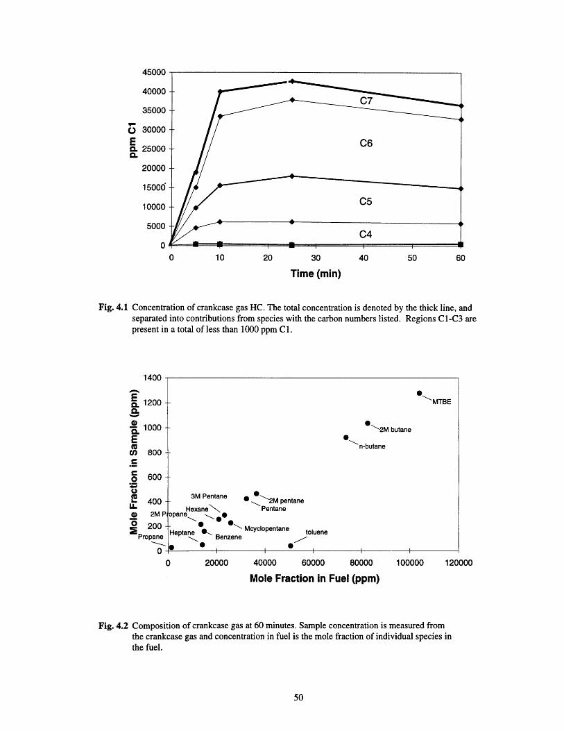
45000
40000
35000
0 30000EC. 25000CL
20000
15000
10000
5000
00 10 20 30 40 50 60
Time (min)
Fig. 4.1 Concentration of crankcase gas HC. The total concentration is denoted by the thick line, andseparated into contributions from species with the carbon numbers listed. Regions C1-C3 arepresent in a total of less than 1000 ppm C1.
1400
.1200 -
1000 -Et) 800 -
o 600-
400-) 2M P
o 200-Propane
V
MTBE
'2M butane
n-butane
0
-3M Pentane
Hexanepane g 0
Heptane ,Benzene
- - 2M pentanePentane
Mcyclopentane toluene
20000 40000 60000 80000 100000 120000
Mole Fraction in Fuel (ppm)
Fig. 4.2 Composition of crankcase gas at 60 minutes. Sample concentration is measured fromthe crankcase gas and concentration in fuel is the mole fraction of individual species inthe fuel.
U
CHAPTER 5
FUEL TRANSPORT MODEL
One of the objectives of this research was to develop a more complete understanding of the
mechanisms for fuel transport within cylinder liner oil layers and throughout the engine. Determining how
much fuel is involved in these processes, differences in transport between fuel species, and how the mass
fluxes of fuel species change during warm-up and steady state is best determined through a simple mixing
model.
5.1 Concept
Fig. 5.1 shows a framework for fuel transport in the oil and crankcase circuits of an internal
combustion engine. The shaded rectangles correspond to control volumes from which fuel species enter and
exit. These control volumes are connected by lines which represent fuel transport from one control volume
to another. Solid lines indicate transport of absorbed fuel species by oil, and dashed lines represent fuel
species mass fluxes in the vapor phase. Mass fractions of fuel species in the control volumes are denoted by
Xi and mass fluxes of fuel species are represented by rhi . During engine operation, fuel is inducted along
with air into each cylinder of the engine. Following the paths in Fig. 5.1, fuel enters the liner oil control
volume as liquid fuel impinging on the liner, or through the fuel absorption process involving cylinder
gases. Sinks of fuel present in liner oil are mechanisms by which fuel leaves the oil. These mechanisms
include desorption of fuel into the cylinder and crankcase gases. The liner oil can also exchange fuel with
blow-by gases, which are in close proximity to ring pack oil. The liner oil is scraped down from the
cylinder each cycle, with a fraction of this oil (and the fuel absorbed therein) carried into the sump oil (Fig.
5.1). Sump oil is pumped along the main crankshaft bearings and then splashed back onto the liner. This
lubrication process of liner and sump oil exchange is one route by which fuel species travel between the
liner oil and sump oil. Fuel can be transported by diffusion between the sump oil and the crankcase gases.
Fig. 5.1 shows blow-by gases carrying fuel components into the crankcase gas for a residence period, after
which they exit through the positive crankcase ventilation (PCV) valve back into the intake system.
5.2 Fuel Transport Model
The focus of the fuel transport model is determining the direction and magnitude of the mass of
fuel species transported between the control volumes of interest: the crankcase gas, the liner oil, and the
sump oil. Individual fuel species mass fluxes and the integrated mass flux of all the fuel species are
examined in the model. In Fig. 5.1, hizsc i is the mass flux of species i transported between the sump and
crankcase. The species mass flux between the liner oil layers and crankcase gas is denoted rhic i . The

mass fluxes rhsc and rhLci can be calculated by applying mass conservation to the species in the sump oil
and liner oil. An estimate of the effect of blow-by gas contribution to fuel species transport can also be
made using thsc and rhLc,. Also in Fig. 5.1 is thepC,, which is the species mass flux from the crankcase
gas to the positive crankcase ventilation valve.
Blow-by gases containing fuel species interact with liner oil films before entering the crankcase.
This study does not include measurements of blow-by gas fuel concentrations near the ring pack. Instead,
the mass fraction of fuel in blow-by is derived from crankcase gas measurements of CO2 described in
section 5.3. Therefore, the mass flux of fuel species in blow-by rhiB , is modeled as entering the crankcase
without interacting with liner oil layers. Blow-by fuel exchange with the liner oil is lumped with the mass
flux of fuel species transported between the crankcase gas and the liner oil layer, rhLCi . The diagram in
Fig. 5.2 reflects these simplifications, and will be used to represent transport processes in the engine oil.
This figure is useful in understanding the discussion of the fuel transport model that follows in the
remainder of this chapter.
5.3 Model Inputs
This section describes various inputs to the fuel transport model that were needed in order to
realistically describe the transport of fuel within the oil and crankcase gases. The areas examined are: the
liner oil layers, oil refreshment rate and oil film thickness.
5.3.1 Liner Oil Layers
The method used to estimate the total volume of oil in the cylinder for this study is based on oil
film thickness (OFT) measurements made by lubrication researchers. The oil film was measured in a
Kohler spark-ignited engine operating at a similar speed and load as the engine in this study, with similar
piston and bore geometry [19]. The Kohler engine used 10W-30 mineral oil, while the engine in this work
operated with 5W-30 mineral oil. Nevertheless, Kohler engine data was used to make estimates of oil film
thickness for the calculations in the fuel transport model. An estimate of the range of OFT on the free liner
and piston skirt is shown for the time periods when the piston is at bottom center, mid-stroke, and top center
(Fig. 5.3). In reality, the OFT can change during engine warm-up, and values may vary depending on
whether the piston is in downstroke or upstroke [20]. The OFT ranges are intended to be wide enough to
account for these and other uncertainties (bore distortion, honing volume, etc.). A simple equation for the
volume of liner oil, Vi, in region i is:
Vi = ;rBSil (5.1)

for a cylinder with bore B, region with oil film thickness 5, and liner length 1. The land and piston geometry
were measured using precision calipers, so that the oil volume there could be accurately calculated. An
expression for the volume of oil on a region of the piston skirt or land with length 1 is
V, = 2r( D-)81 (5.2)
where D is the diameter of the piston.
The volume of oil in the ring pack is approximated as constant for all time and piston positions.
The estimated volume of oil on the lands and in the ring grooves, along with dimensions used in OFT
calculations are shown in Fig. 5.4. The amount of oil in the ring grooves is calculated by estimating what
fraction of each groove is flooded, excluding the piston ring volume. The volume of oil in a particular ring
groove can be estimated as
V = 27rtphd( -d) (5.3)2
for a piston of diameter D, groove height h, groove depth d, and flooded fraction Tp. Using these estimates,
the total volume of oil in one cylinder was calculated to be approximately 2 cm 3. The largest contribution to
the total volume of oil is from the flooded oil control ring groove and the lower liner, which together make
up almost 1.6 cm3 .
Calculating the volume of oil on the liner is necessary in order to evaluate the mass of fuel species
from measured concentration data. If an accurate value for the volume (and subsequently the mass) of the
oil is known, the mass of the fuel species on the liner at a given time can be evaluated from GC
measurements of the mass fraction of fuel species in oil. The oil film on the liner was modeled as a well-
stirred volume of oil consisting of the regions described above. The assumption of thorough mixing along
the length of the liner is assumed to be valid for the time scale at which oil was sampled [20]. Therefore,
fuel concentrations in oil sampled from the piston skirt region may be considered representative of values
throughout the liner oil layer. It is assumed that fuel concentrations are not varying circumferentially
around the liner, nor from cylinder to cylinder. These simplifications were partly supported by
measurements made on opposite sides of the piston (Chapter 3). The oil films which coat the cylinder head
were not considered in this study, since their participation in transport processes is likely to be small.
The viscosity of oil on the liner decreases with increasing engine temperature during the warm-up
phase. The decrease in oil viscosity reduces the oil film thickness and therefore, the total volume of oil on
the liner may be over-predicted [15]. Absorbed fuel has a smaller effect on the decrease of oil viscosity.
Both of these phenomena were not modeled since they are of little importance in the regions that contribute
the largest volume of oil to the cylinder: the lower liner oil and oil control ring groove.

5.3.2 Oil Refreshment Rate
An important input to the fuel transport model is the mass flow rate of oil between the sump and
the liner oil layers, mhoil (Fig. 5.5). This oil exchange rate can be expressed as the percentage of the mass of
cylinder liner oil that is replaced each revolution, which is termed the refreshment rate, R. This calculation
requires a value for the mass of liner oil (Section 5.3.1). The refreshment rate is calculated by using sump
and liner oil HC species measurements of absorbed heavy fuel species during the first 10 minutes of engine
operation. At this time, the engine coolant and oil are relatively cool, so high molecular weight fuel species
are unlikely to be transported in the gas phase (rhsc,, htLC, = 0). During this period, it was assumed that
the only flux of heavy fuel species into and out of the sump oil is by absorbed fuel in the flow of oil between
the sump and liner (Fig. 5.5). Applying mass conservation to species i in the sump oil results in
dX4thoil(XLi - Xsi)= M s (5.4)
where Fhoil is the mass flow rate of oil between the liner and sump for one cylinder, Xt, and Xs, are the
mass fractions of fuel species i in the oil, and Ms is the mass of sump oil. The mass fractions X4 and
X s, are obtained from the measurements of 1,2,4-trimethylbenzene and naphthalene discussed in Chapter 3
and shown in Figs. 3.4 and 3.5. A factor of four is included in Eq. 5.4 since the oil from four cylinders is
being exchanged with sump oil. The refreshment rate R is defined as
R = mril (5.5)M. N
where N is engine speed. The calculated refreshment rate (Fig. 5.6) is between 1% and 3%, depending on
the fuel species mass fractions used as input to Eqs. 54 and 5.5. Using naphthalene fuel concentrations as
an input results in a constant refreshment value of 1.25%. The refreshment rate calculated using 1,2,4-
trimethylbenzene measurements is not constant, probably due to gas transport with the crankcase gases.
The calculated refreshment rate agrees well with Norris' estimate of refreshment rate, which adds
confidence to the estimate of liner oil volume discussed in Section 5.3.1 [8].
5.3.3 Blow-by Gas
In order to model fuel transport to or from the crankcase gas, the rate at which blow-by gas enters
and exits the crankcase is needed. The engine used in this study had no fresh air dilution to the crankcase
gases, since the fresh air hose was sealed (Fig 5.7). Therefore, when the crankcase is sufficiently filled with
gas, the flow rate leaving the PCV valve is equal to the flow rate of blow-by. A simple experiment was
conducted to measure the volume flow rate of crankcase gas exiting through the PCV hose. A tube attached

to the end of the PCV hose was immersed in a tank of water (Fig. 5.8). The volume of water displaced
when the engine is operating is then equal to the blow-by flow rate into the crankcase. The measured flow-
rate of blow-by into the crankcase at start-up was 12 L/min, which corresponds to 2.6% of the charge.
Blow-by was reduced to 6 L/min after 5 minutes, which may be the result of better sealing between the
piston rings and liner as the engine warmed. These values compare favorably with measurements made by
previous researchers on similar engines [4]. The mass flow rate of blow-by is calculated by multiplying the
measured volume flow rate by the density of air at the measured crankcase temperature of 60 'C and
pressure of 33 kPa (absolute).
The mass flux of fuel species in the blow-by gas is rhBc (Fig. 5.2). The concentration of CO 2 was
measured in the crankcase gas to determine rhBc . The crankcase CO2 concentrations rise to a steady state
concentration of 2.25% after five minutes. This is the time required to fill the crankcase with combustion
gas CO2, which diffuses out of the crankcase after the engine is stopped. As described above, the crankcase
is a closed circuit with no fresh air dilution. Therefore, the only source of CO 2 to the crankcase is from
blow-by. Comparing the concentration of CO 2 in the crankcase gas with the amount present in the cylinder,
an estimate of the fraction of charge in blow-by can be made.
The mass fraction of residual gas in typical four valve engines operating at the engine conditions of
this study is approximately 15% [4]. It was assumed that the residual gas in the cylinder contains the same
concentration of CO 2 as exhaust gas. The cylinder always contains the CO 2 present in the residual gas. The
mass fraction of CO2 present in unburned charge is negligible (3.104). Depending on the crank angle there
will also be CO2 in the cylinder present from the cylinder burned gas. The cylinder concentration of CO2 at
a specific point in a cycle can thus be expressed as:
= fr (XC 2 )+(-(fch + f,))Xco2 (5.6)
where fr is the cylinder residual mass fraction, X co2 is the mass fraction of CO2 in burned cylinder gases,
and fch is the mass fraction of unburned charge in the cylinder. In a simplification of the blow-by process,
we assume that the measured crankcase concentration of CO2 is equal to X c when blow-by occurs. The
only unknown in Eq. 5.6 is fch, the fraction of unburned charge in the cylinder when blow-by occurs, which
therefore, is the fraction of charge in blow-by. Solving Eq. 5.6 for fch yields 86% for the fraction of charge
in blow-by. This result is consistent with the distribution of fuel components observed in the crankcase
sampling of Chapter 4.
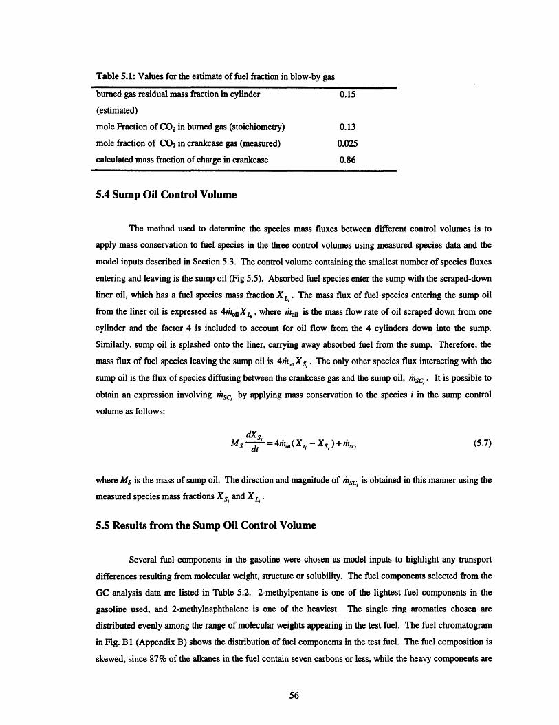
Table 5.1: Values for the estimate of fuel fraction in blow-by gas
burned gas residual mass fraction in cylinder 0.15
(estimated)
mole Fraction of CO2 in burned gas (stoichiometry) 0.13
mole fraction of CO2 in crankcase gas (measured) 0.025
calculated mass fraction of charge in crankcase 0.86
5.4 Sump Oil Control Volume
The method used to determine the species mass fluxes between different control volumes is to
apply mass conservation to fuel species in the three control volumes using measured species data and the
model inputs described in Section 5.3. The control volume containing the smallest number of species fluxes
entering and leaving is the sump oil (Fig 5.5). Absorbed fuel species enter the sump with the scraped-down
liner oil, which has a fuel species mass fraction Xi . The mass flux of fuel species entering the sump oil
from the liner oil is expressed as 4ith0i X , where thoil is the mass flow rate of oil scraped down from one
cylinder and the factor 4 is included to account for oil flow from the 4 cylinders down into the sump.
Similarly, sump oil is splashed onto the liner, carrying away absorbed fuel from the sump. Therefore, the
mass flux of fuel species leaving the sump oil is 4th, Xsi . The only other species flux interacting with the
sump oil is the flux of species diffusing between the crankcase gas and the sump oil, rhsc. It is possible to
obtain an expression involving thsc, by applying mass conservation to the species i in the sump control
volume as follows:
dXs
Ms = 4rth,(X - Xs,)+rhsc (5.7)
where Ms is the mass of sump oil. The direction and magnitude of thsc, is obtained in this manner using the
measured species mass fractions Xs, and X4 .
5.5 Results from the Sump Oil Control Volume
Several fuel components in the gasoline were chosen as model inputs to highlight any transport
differences resulting from molecular weight, structure or solubility. The fuel components selected from the
GC analysis data are listed in Table 5.2. 2-methylpentane is one of the lightest fuel components in the
gasoline used, and 2-methylnaphthalene is one of the heaviest. The single ring aromatics chosen are
distributed evenly among the range of molecular weights appearing in the test fuel. The fuel chromatogram
in Fig. B 1 (Appendix B) shows the distribution of fuel components in the test fuel. The fuel composition is
skewed, since 87% of the alkanes in the fuel contain seven carbons or less, while the heavy components are

mostly aromatic species. 'Total fuel HC' in Table 5.2 is the mass fraction of all fuel species in each oil
sample, obtained by integrating the areas of all fuel species in a sample chromatogram. Using this integrated
data as an input to the calculations in this section gives averaged mass fluxes for all the fuel species in the
oil. The fuel species in Table 5.2 were also chosen because they were present in sufficient quantities in the
oil to make accurate measurements.
Table 5.2 Fuel components chosen as modeling inputs
Fuel Component Chemical Group Molecular Weight(g/mol)
2-methylpentane Alkane 86.18
toluene Aromatic 92.14
xylenes Aromatic 106.17
1,2,4-trimethylbenzene Aromatic 120.20
2-methylnaphthalene Aromatic (PAH) 142.20
total fuel HC Alkanes, Aromatics, Olefins, Ethers
The results obtained in the sump control volume are the magnitude and direction of rhsci , the mass
flux of species i between the crankcase gas and the sump oil. The species mass flux rhsc, is determined by
solving Eq. 5.7. The input mass fractions Xsi and XL4 are obtained from the oil sampling experiments
described in Chapter 3 (Figs. 3.10-3.13). A polynomial curve fit is used for the species mass fractions in
each of the data plots resulting in the curve-fit data used as an input to Eq. 5.7 (Fig. 5.9). The curve fits
smooth the data to allow for the differentiation in Eq. 5.7. In this manner, rzsc, was computed for the fuel
species of interest. The magnitude of the species mass flux rhsc, was then normalized by the rate that each
of the species is injected into the cylinder during stoichiometric engine operation, rhiji . The corresponding
fraction, rhsc / rji is shown in Fig 5.10.
An average transport rate and direction for all fuel species is given by inputting the total fuel HC
mass fractions Xs and XL into Eq. 5.7. Recall that the total fuel HC is the sum of all the fuel species in the
gasoline. For the total fuel HC (Fig. 5.10), rhsc is always directed from the crankcase gas to the sump and
x/4 rnj increases from 0.3% at 10 minutes, to 1.6% after 3 hours. During warm-up, this ratio is low except
for a sharp peak during the first 5-10 minutes. In Eq. 5.7, this peak results from the liner fuel concentration
increasing at a rate which is not high enough to account for the increase in sump oil. The validity of the
first sampling points (at 2.5 minutes and 5 minutes) may influence calculations during this time period.
Another small peak in mtsc/ kjis shown in Fig. 5.10 at approximately 25 minutes, and can also be seen in
the liner species mass fractions in Fig. 5.9.
The evolution of rhsc for the total fuel HC is similar to that of the individual fuel species (Fig. 5.10).
The fuel species shown are ordered by increasing molecular weight from right to left, and from bottom to
top. For the fuel components shown, the magnitude of rsci / fi j, after warm up generally increases with
molecular weight. The species mass flux rhsc is directed from the crankcase gas to the sump oil for all of
the species for most of the three hour engine running time. In Fig. 5.10, 1,2,4-trimethylbenzene is the only
species with hic directed from the sump oil to the crankcase gas between 100 and 150 minutes of engine
operation.
The magnitude of itsc / Ir i ji is substantially higher for 2-methylnaphthalene compared to the total
fuel HC and the other fuel species. At three hours of engine operation, 2-methylnaphthalene is transported
to the sump oil from the crankcase gas at 13% of the rate that 2-methylnaphthalene is injected into the
cylinders (Fig. 5.10). This can partly be extracted from 2-methylnaphthalene data in Fig. 5.9, where the
sump oil mass fraction of 2-methylnaphthalene is larger than the liner oil mass fraction. Additionally, the
slope of the mass fraction of 2-methylnaphthalene (dXs/dt) in the sump oil is high. Both of these factors
increase the magnitude of rhsci in Eq. 5.7. Finally, since 2-methylnaphthalene is less than 1% of the
injected fuel, the ratio rhsci/fnji is also high. It is unlikely that the inputs Xs, and XL4 in Eq. 5.7 are in
error, since 2-methylnaphthalene mass fractions in oil do not deviate from other absorbed fuels of similar
molecular weight, as seen in Chapter 3 (Fig. 3.19). This large magnitude of thsci does not appear to be a
characteristic of polynuclear aromatic hydrocarbon transport, either. The same normalized fluxes
calculated for naphthalene are approximately 3% of the injected amount at three hours. The high boiling
points of the heavy fuel species may be responsible for their higher percentage in the engine oil.
The time necessary for the species mass flux thsc, to reach a steady state is the same as that
required for the fuel concentrations in the oil to reach steady state. Therefore, risc approaches steady state
within three hours for 2-methylpentane, toluene and xylene, while Phsq is still increasing for the other fuel
species. Since heavy fuel species make up a large percentage of the fuel in the oil, the plots of thsci / rnjiin Fig. 5.10 for the heavier fuel components bear a strong resemblance to the same plot for the total fuel
HC. Except for the high magnitude of 2-methylnaphthalene transport, the species mass flux from crankcase
gas to the sump oil appears to be a fairly consistent process across all the fuel species examined.
5.6 Liner Oil Control Volume
The fluxes of fuel species interacting with the liner oil control volume are more complicated than
those encountered with the sump oil control volume (Fig. 5.12). Again, oil is splashed up from the sump
generating a species mass flux of absorbed fuel components to one cylinder liner. This flux can be
expressed as hoil Xsi . As discussed for the sump oil control volume, the liner oil is scraped down from the
cylinder, which represents a fuel species mass flux out of the liner. This flux term is rioil X 4 . The liner oil
control volume consists of only the oil in one of the four engine cylinders, so the mass fluxes are not
multiplied by 4 as in the sump oil control volume. Fuel species in the liner oil layer are absorbed and
desorbed between the cylinder gas, the crankcase gas and blow-by. As shown in Fig. 5.12, rihLi is the
species mass flux between the crankcase gases and the liner oil. Also lumped in rnhLC is the flux between
the blow-by gas and the liner oil. The remaining flux term in Fig. 5.12 is rhabs, . The mass species flux
mabsi groups the species mass fluxes from absorption and desorption of cylinder gases (not including blow-
by), as well as the species mass fluxes from oil consumption and liquid fuel impingement. It is possible for
riabs, to be positive or negative depending on the magnitude of the individual species mass fluxes. The
terms appearing in the conservation of the mass of fuel species i in the liner oil are
dXLM L -- L = hoil(Xsi - XC, )+ hLC, + tmabsi (5.8)
where ML is the mass of oil on the liner. The unknown terms in Eq. 5.12 are rILc, and thabs. . Again
grouping the unknown fluxes together, Eq. 5.8 becomes
dXML L - thoil(Xsi - Xc )+thnet (5.9)
where rhneti is the net mass flux of species absorbed in the liner oil, excluding the contributions of fuel
transport by rioil .
5.7 Results from the Liner Oil Control Volume
The flux calculated in this section, izet,, is the net (non-oil transport) fuel species interaction with
the liner oil layer. Eq. 5.9 is used to calculate rneti , and the inputs to Eq. 5.9, Xsi and XL4 are again from
the curve-fit experimental data in Fig. 5.9. The magnitude of thneti for each of the species in Table 5.2 is
again normalized by the rate that each of the species is injected into the cylinder during stoichiometric
engine operation, 6tinj, . The ratio (rhnet, / 1inji ) is plotted in Fig. 5.11.
The integrated fuel species value of rihnet is examined first. The total fuel HC plot in Fig. 5.11
shows that the mass flux thnet is towards the liner oil layer during the first 70 minutes of engine operation.
For this time period, there is a net flux of total fuel HC from blow-by, crankcase gas, cylinder gas and liquid
fuel impingement to the liner oil. After this point, the direction of the net mass flux changes, and itnet is
negative, based on the sign convention used in Eq. 5.9. This corresponds to a mass flux of total fuel HC
from the liner oil which is apportioned to the cylinder gas, crankcase gas, or blow-by. The ratio

rhnet / ti nj is less than 2% for the three hour engine test duration. This ratio is about 1.8% after ten minutes
and decreases steadily until it reaches -1.8% after three hours of engine operation.
The species mass fluxes thneti share similar characteristics to thnet for the total fuel HC. The
species mass fluxes rhneti are initially positive, at which time the rhneti becomes negative (and the liner oil
becomes a source of fuel species) varies depending on the molecular weight of the fuel species. For
instance, in Fig. 5.11, rhneti is negative for 2-methylpentane after 10 minutes of engine operation, while it
remains positive for 1,2,4-trimethylbenzene until nearly 180 minutes. The sign change in rnneti occurs
approximately when Xsi is equal to XL4 in Eq. 5.9, which is also visible in Fig. 5.9. The magnitude for 2-
methylnaphthalene transport is again higher than for other species, with rhnet ,il/inji changing from 8% to -
8% over the duration of the test (Fig. 5.11). The species mass flux rhneti is nearly zero for 2-methylpentane
for the three hours of engine operation. This indicates that the transport mechanisms grouped in thneti do
not involve the light paraffins, or that the processes in thneti are offsetting each other.
5.8 Crankcase Gas Control Volume
The model of fuel transport between the crankcase gas and the engine oil is structured in a similar
manner to the model of fuel species interaction with the liner and sump oil. A crankcase gas control volume
is defined with mass fluxes of fuel species interacting with the control volume. Through mass conservation
of the species in the crankcase control volume, additional information about the species mass fluxes
interacting with the engine oil is obtained (Fig. 5.13). The species mass flux of fuel between the crankcase
gas and the sump oil, thsci was already calculated in section 5.6 using Eq. 5.7 and oil sampling data. There
are three other fluxes interacting with the crankcase gas: rhpcv, mhc, and rhBcj . The species mass flux
thLC, is the transport of fuel species between the liner oil layer and both the crankcase gas and blow-by.
The term rhzBc is the species mass flux entering the crankcase gas from blow-by. The species which exit the
crankcase via the PCV valve are represented by rhzpcv.. Both rhpcv, and rhBc, were determined
experimentally. Under steady state conditions, the species mass flux rhBci through the PCV valve can be
expressed as
rhBC, = fch hBBWi (5.10)
where fch is the mass fraction of charge in blow-by, rhBB is the mass flow rate of blow-by gas in the
crankcase, and wi is the mass fraction of fuel species i in the charge. Section 5.3.3 described the technique

used to calculate fch and the volume flow rate of blow-by. The mass fraction wi is obtained from
stoichiometry and GC analysis of the total fuel. The species mass flux rhpcvi is
rhpcvi =-'BB Xcc, (5.11)
where Xcc, is the mass fraction of fuel species i in the crankcase gas. The mass flow rate rhBB is constant
for both Eqs. 5.10 and 5.11. Applying mass conservation to the species in the crankcase control volume
(Fig. 5.13) produces the expression
dX c c,(5.12)Mcc dt mBc, -m sc -m iLC -rcv (5.12)
where Mcc is the mass of crankcase gases. This expression can be solved for rhLc, so the crankcase gas and
blow-by gas contribution to liner oil transport can be determined. In section 5.7, ihneti was determined as
the sum of ,hjc and rhabsi. Therefore, solving Eq. 5.12 for rhtLC gives the magnitude of ihabs, the flux
term described in section 5.6. While rhsc, in Eq. 5.12 is dependent on the results of the sump control
volume, the other terms are independent of the previous calculations involving the engine oil.
5.9 Results from the Crankcase Gas Control Volume
The term discussed in this section is the species mass flux minLc, calculated by solving Eq. 5.12.
The inputs into this equation are the measured species mass fractions in the liner and sump oil, the measured
crankcase gas species mass fractions, and the species mass flux riBCi and rhpcv, described in Section 5.8.
A polynomial curve fit was again applied to the crankcase gas concentrations cc, and is shown in Fig. 5.14.
In Fig. 5.15 the ratio thLC; /rhinji is plotted for 2-methylpentane and toluene along with the previously
calculated tihnet / rinj, . For 2-methylpentane, the direction of rhtc, is negative, transport is from the liner oil
layer to either the crankcase gas or blow-by. The magnitude of ritc, /irinj, ranges between -1.4% and 0%
during the 60 minutes of engine operation for which input data to Eq. 5.12 is available. Since ihneti is the
sum of rhiC and Irhbsi, Fig. 5.15 shows that for 2-methylpentane the direction of hnab,i must be to the liner
in order for rinet i / rinij, to be nearly zero.
Solving Eq. 5.12 with toluene as the input fuel species, it is determined that the mass flux rhtiLC is
directed to the liner oil layer. This direction is opposite of what was observed with 2-methylpentane. The
magnitude of rhtLC / hinji varies between 0% and 1%, with the irregularity in Fig. 5.15 coming as a result of
the changes in ihsci observed in Fig. 5.10. The plots of rhZLC /lhinj, and rinet /rilinji in Fig. 5.15 are nearly
identical for toluene during the first 25 minutes. For this warm-up period, the species mass flux Ihabsi is
nearly zero. After this time, the magnitude of rhLC / rinj, is about 1% higher than hnet / rinj, , which means
that thabs is negative, and the liner oil acts a source of fuel species to the cylinder gases.
Complete box diagrams of the light, intermediate, and heavy species fluxes discussed in Sections
5.4-5.9 are shown in Figs. 5.16-5.17. The box diagrams are arranged similar to Fig. 5.2, which gives the
species fluxes between the three control volumes of interest. In Fig. 5.16, the species mass fluxes at the end
of warm-up (approximately 30 minutes) are shown. The species fluxes immediately to the right of the liner
oil are rizn•t, the total (non-oil) transport to the liner oil. The two species fluxes to the left of the crankcase
gas control volume are the species fluxes rhLc, the species mass flux between the liner oil layer and both
the crankcase gas and blow-by gas. Fig. 5.17 is a similar box diagram for three hours of engine operation.
Figure 5.18 is a box diagram comparing the total fuel mass fluxes at warm-up and steady state. Particularly
evident in the box diagrams of the individual fuel species (Figs. 5.16-5.17) is the role of liner oil layers as
sources of light hydrocarbons to the crankcase gas, and the build-up of heavy hydrocarbons in the sump oil.
5.10 Uncertainty Analysis
In order to model the transport of fuel in the oil and crankcase gases, simplifications, experimental
measurements, and assumptions were made which introduce uncertainty into the results. As discussed in
section 5.3, there were a number of assumptions made concerning the oil layer thickness and distribution in
the cylinder. These assumptions affect the calculated mass of fuel species in the oil, and therefore
propagate uncertainty in calculations involving this term. The uncertainty in gas chromatography analysis of
experimental data, while minimized by frequent calibration, was also estimated. Errors in the structure of
the model, such as neglect of a transport route or attributing a single flux to the result of a number of fluxes,
usually lead to inconsistencies in a model. One purpose of the crankcase gas calculations, which were not
completely dependent on oil sampling data, was a consistency check with other model calculations. Since
the mass fluxes calculated using crankcase gas data are, for instance, not greater than the amount of fuel
injected, it is unlikely that a major error in model structure is present.
In Table 5.3, the uncertainties associated with model inputs are listed. These terms are the inputs
to Eqs. 5.7, 5.9 and 5.12. The value used for the volume of oil on the cylinder liner was 2 cm3, based on the
analysis of Section 5.3. The liner oil refreshment rate calculated using the estimated liner oil volume also
agreed well with other studies. Varying the bounds on oil film thickness from the lowest values seen in the
Kohler experiments to the highest values [19,20], it is likely the volume of oil is between 2.25 cm3 and 1.75
cm3. It is not unusual, however, for uncertainty in the cylinder oil volume to range as high as ±50%. Using
the bounds mentioned above, the fractional uncertainty in the liner oil mass ML is ±12.5%. Based on sample
repeatability and a calibration sample, the fractional uncertainty in GC measurements, and therefore XL and
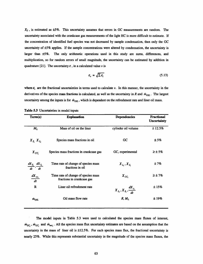
Xs, is estimated as ±5%. This uncertainty assumes that errors in GC measurements are random. The
uncertainty associated with the crankcase gas measurements of the light HC is more difficult to estimate. If
the concentration of identified fuel species was not decreased by sample condensation, then only the GC
uncertainty of ±5% applies. If the sample concentrations were altered by condensation, the uncertainty is
larger than ±5%. The only arithmetic operations used in this study are sums, differences, and
multiplication, so for random errors of small magnitude, the uncertainty can be estimated by addition in
quadrature [21]. The uncertainty E , in a calculated value v is
EV = j (5.13)
where ei are the fractional uncertainties in terms used to calculate v. In this manner, the uncertainty in the
derivatives of the species mass fractions is calculated, as well as the uncertainty in R and rhorL . The largest
uncertainty among the inputs is for rhoIL, which is dependent on the refreshment rate and liner oil mass.
Table 5.3 Uncertainties in model inputs
Term(s) Explanation Dependencies
Mass of oil on the liner
Species mass fractions in oil
Species mass fractions in crankcase gas
Time rate of change of species massfractions in oil
Time rate of change of species massfractions in crankcase gas
Liner oil refreshment rate
Oil mass flow rate
cylinder oil volume
GC
GC, experimental
X , X si
dXtX ,,X, dt
R, ML
The model inputs in Table 5.3 were used to calculated the species mass fluxes of interest,
thsc4 , rktc, and .rne. All the species mass flux uncertainty estimates are based on the assumption that the
uncertainty in the mass of liner oil is ±12.5%. For each species mass flux, the fractional uncertainty is
nearly 25%. While this represents substantial uncertainty in the magnitude of the species mass fluxes, the
FractionalUncertainty
ML
Xsi X4
X cc,
dX s dX 4dt ' dt
dX Ccdt
R
rhoIL
± 12.5%
±5%
±7%
± 15%
± 19%

directions and approximate magnitudes of all the fluxes remain unchanged. For example, rhsc i , which is
the species mass flux from the crankcase gas to the sump oil, has a fractional uncertainty of ± 22%. For
toluene (Fig. 5.10), this means rhsc, / thinj, at 180 minutes is between 1.32% and 0.88%. The calculated
uncertainty for rhiz, is greater than or equal to 23% because of the uncertainty in X cc and the estimates of
blow-by flow rate and fraction of charge in blow-by. An example of a calculated species flux with the
uncertainty bounds of Table 5.4 is shown in Fig. 5.19.
Table 5.4 Uncertainties in calculated species mass fluxes
Species Explanation Dependencies FractionalMass Flux Uncertainty
rhsci Crankcase gas to sump oil flux dXS + 22%X q' X s I- , Mrit
mrLCi Crankcase and blow-by gas to liner oil dX cc, + 23%flux dt rmsc, , others
th,•ti hLc, and thabs, X 4 , M dX OIL ± 25%
5.13 Conclusions
In this chapter, a framework for the mass transport of fuel species between the crankcase gas, sump
oil and liner oil was presented. In order to calculate species mass fluxes of interest, several parameters
needed to construct a fuel transport model were calculated. The liner oil refreshment rate was estimated
from experimental data, as was the concentration of fuel species in blow-by gas. Species balances involving
the mass fluxes interacting with the engine oil and crankcase gas were applied to appropriate control
volumes to obtain mass fluxes. The control volumes established were the liner oil, sump oil and crankcase
gas. The species mass fluxes between the crankcase gas and sump oil were determined, as were the mass
fluxes between the liner oil and both the crankcase and blow-by gas. The mass fluxes describing the net
interaction of the liner oil layer with the mechanisms of liquid fuel impingement, and absorption and
desorption to cylinder, crankcase, and blow-by gases were also calculated. These mass fluxes were
determined during warm-up conditions and up to 180 minutes of operation. Five fuel species which span
the molecular weight range of the test fuel were chosen as model inputs, along with the total fuel
concentration in oil. The fuel concentrations were obtained from the oil sampling and analysis described in
previous chapters.
The calculations described in this chapter show that there are species mass fluxes from the
crankcase gas to the sump oil which increase with engine operating time, until steady state concentrations of

fuel in oil are reached. These mass fluxes are generally larger in magnitude for higher molecular weight
fuel species and varied from 0% to 14% of the rate at which individual fuel species are injected into the
cylinder during stoichiometric operation. From calculations involving the mass fluxes interacting with the
liner oil layer, it was determined that for each of the species modeled during warm-up, there is a net flux of
fuel species to the liner oil from cylinder, crankcase and blow-by gas fuel species as well as possibly liquid
fuel species impinging on the liner. The direction of this mass flux reverses at the point when the
concentration of fuel in the liner oil is equal to that in the sump oil. Using crankcase gas data of 2-
methylpentane and toluene, the mass fluxes between the liner oil and both the crankcase and blow-by gas
were calculated. For 2-methylpentane after 20 minutes, the direction of fuel transport was from the liner oil
layer to the crankcase gas and blow-by gas, with a magnitude of nearly 1% of the stoichiometric rate of 2-
methylpentane injection. For toluene, the calculated direction of species transport was from the crankcase
gases and blow-by to the liner oil layer, with approximately 0.6% of the rate of injected toluene transported
in this manner. In addition, for steady state, the amount of toluene desorbing to the cylinder gas was
calculated to be 0.6% of the rate of injected toluene. It is evident from examining different classes of fuel
species, that the liner oil is a source of light hydrocarbons to the crankcase gases and blow-by, while the
sump oil is a sink for the heavy fuel species.

FUEL INJECTED
SOURCES
SINKS ......
BLOW-BY BURNED
mBL, mBC;'..
mLCi4 --o•. ---
trnoloT
Fig. 5.1 Framework for fuel transport in engine oil. Italicized symbols are mass fluxes of fuel species.Dashed lines represent fuel transport in the gas phase between shaded control volumes, and solidlines indicate transport by oil. The mass flux ihrcvi is recycled to the intake manifold.
FUEL INJECTED
NET SOURCES
mI abs
BLOW-BY BURNED
mBC.
mLCi-4. ..............
Fig. 5.2 Simplified fuel transport framework. Note particularly the change in how blow-by gasexchange is modeled.
. . .. .. 1 1 - 11 i i .. .
. A
MTqj
······.|
msc
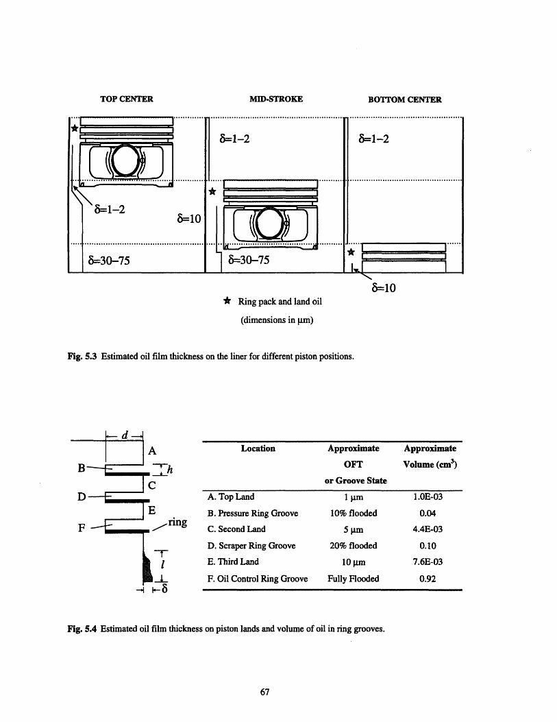
BOTTOM CENTER
6= 10*" Ring pack and land oil
(dimensions in gtm)
Fig. 5.3 Estimated oil film thickness on the liner for different piston positions.
Location
i-h
A. Top Land
B. Pressure Ring Groovenring C. Second Land
D. Scraper Ring Groove-f-1 E. Third Land
_L. F. Oil Control Ring Groove
Approximate
OFT
or Groove State
1 Rm
10% flooded
5 gim
20% flooded
10 Pm
Fully Flooded
Approximate
Volume (cm3)
1.0E-03
0.04
4.4E-03
0.10
7.6E-03
0.92
Fig. 5.4 Estimated oil film thickness on piston lands and volume of oil in ring grooves.
- 1--O
TOP CENTER MID-STROKE

4 rnoXL, I-, - insc
Fig. 5.5 Sump oil control volume with interacting species fluxes. XL4 and Xs, are the mass fractions
of fuel species i in the liner and sump oil, respectively. ML and Ms are the masses of the liner
oil and sump oil. The crankcase to sump mass species flux is rhsc , and the mass flow rate of
oil between the liner and sump is thiji .
4.0
3.0
2.0
1.0
0.00 5 10
Time (min)
Fig. 5.6 Calculated results for the oil refreshment rate.
i- - -- I- ·- -·---- I · --
T~t-hoilxs

Fig. 5.7 Positive crankcase ventilation system in the Saturn 1.9 L engine. The fresh air hose marked '3' issealed in the test engine. Blow-by past the piston rings is shown, as is the route by which r6rcv,enters the intake manifold at '1' (Saturn engine manual).
graduated cylinder
...........
crankcase gases from
water
PCV Tube
Fig. 5.8 Schematic of experimental setup to measure blow-by gas flow rate.
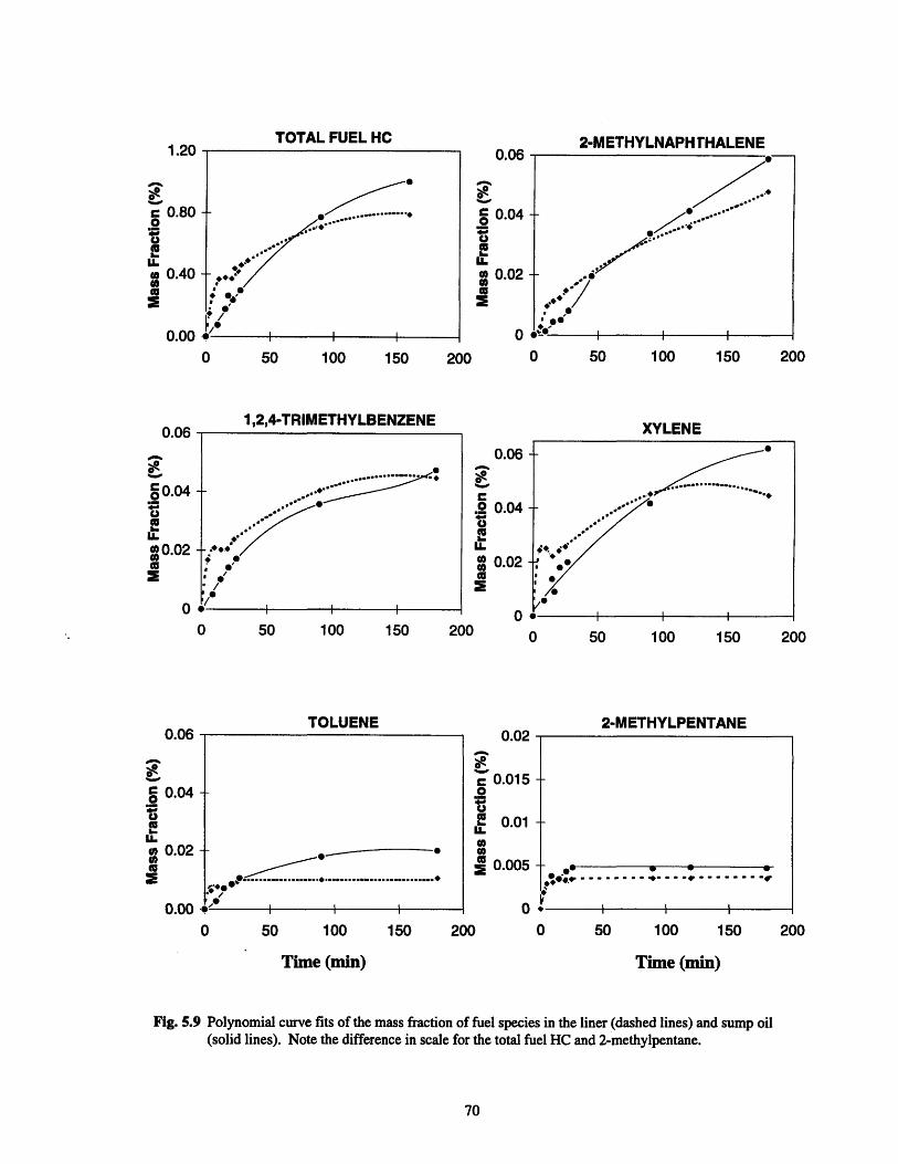
2-METHYLNAPH THALENE0.06
C 0.04
3 0.020
0 50 100 150 200 0 50 100 150 200
1,2,4-TRIMETHYLBENZENE
0 50 100 150
TOLUENE
0 50 100 150
0.06
.2 0.04
0.02
0 0.02
200
XYLENE
I I I
0 50 100 150
0.02
0.015
0.01
0.005
200
200
2-METHYLPENTANE
-
k-
* I I I
0 50 100 150 200
Time (min) Time (min)
Fig. 5.9 Polynomial curve fits of the mass fraction of fuel species in the liner (dashed lines) and sump oil(solid lines). Note the difference in scale for the total fuel HC and 2-methylpentane.
1.20
c 0.800
* 0.40
0.00
0.06
=0.04
U.
00.02
0
0.06
C 0.040
a.
0 0.02
0.00
..-.. . .
TOTAL FUEL HC
-S!I

2-METHYLNAPHTHALENE18.0
0 50 100
12.0
. 6.0
0.0
-6.0
150 200 0 50 100 150
1,2,4-TRIMETHYLBENZENE
0 50 100 150
6.0
4.0
E 2.0
0.0
-2.0
200
TOLUENE
XYLENE
0 50 100
0 50 100
6.0
4.0
E 2.0
E 0.0
-2.00 50 100 150 200
Time (min) Time (min)
Fig. 5.10 Calculated crankcase gas to sump oil species mass flux rhsc,, normalized by the rate each fuelspecies is injected into the engine during stoichiometric operation. A positive izhsci t hinjiindicates fuel species mass transport to the sump oil.
1.2
~ 0.8
E 0.4
0200
71
6.0
4.0
S2.0
0.0
-2.0
6.0
4.0
E 2.0
-20.0
-2.0
150 200
2-METHYLPENTANE
150 200
TOTAL FUEL1.6

TOTAL FUEL
0 50 100 150 200
1,2,4-TRIMETHYLBENZENE
10.0
2.0
-6.0
-14.0
2-METHY LNAPHTHALENE
0 50 100 150 200
4.0
2.0
E
0.0
-2.0
XYLENE
0 50 100 150 200
TOLUENE
0 50 100
Time (min)
4.00
2.00
t 0.00
-2.00150 200
0 50 100 150 200
2-METHYLPENTANE
0 50 100 150 200Time (min)
Fig. 5.11 Calculated liner oil fuel species mass flux mhneti normalized by the rate each fuel species is
injected into the engine during stoichiometric operation. A positive lmneti / fi.nji indicates
fuel species mass transport to the liner oil.
4.0
2.0
, 0.0
-2.0
4.0
2.0
0.0
-2.0
4.0
' 2.0
0.0
-2.0

absorption/desorption between oil and cylinder gas
mabsi oil consumptioni liquid fuel impingement
mLCi............. ,
oil Si
Fig. 5.12 Liner oil control volume with interacting species mass fluxes.
mBCi
1mLCi°,°,. .,,°
Fig. 5.13 Crankcase gas control volume with interacting species mass fluxes.
73
onX L
C -- r -I.-~-----r --- --- ···-·· sl
mpcv.I
MS~

U.ZV
0.15
o 0.10x
0.05
0.00
0 10 20 30 40 50
Time (min)
Fig. 5.14 Curve fit of the crankcase gas mass fractions of toluene and 2-methylpentane.
2-METHYLPENTANE
rnLCj / minji ....
Ihneti / inji
I I
2
r 16ESo
0 -2z
Time (min)
TOLUENE
0 20 40
Time (min)
Fig. 5.15 Calculated values rhLc, / rhinj, and that, / mij, for toluene and 2-methylpentane. Positive
values indicates fuel species mass transport to the liner oil.
60
62
a 0m
o -2z
A AA
.I

0.8%
0.6%
1.3% mid
mid 1
6%
heavy
A..195%- 7%
0% .
..0.2%0.6%- 1%
0.6%- 1%
0.4%- 0.6%
BLOW-BY
2%
3%- 5%
heavy
12%A0.4%- 0.6%
0.4%- 0.6%2-methylnaphthalene
toluene
2-methylpentane
Fig. 5.16 Species mass fluxes for light, intermediate, and heavy fuel species at the end of warm-up (30minutes). The percentages shown are species fluxes normalized by the rate of injection of eachfuel species during stoichiometric engine operation. The range in value for a particular speciesflux corresponds to the likely uncertainty in a species flux. The species flux to the right of theliner oil is the net (non-oil) fuel species transport to the liner oil. The species flux to the left ofthe crankcase gas is the species flux between the liner oil layer and both the crankcase gas andblow-by gas.
........ * 1%
PCV
-^- - - ~-~--~~~--~- ' - i I -p-r r -' -1 5

0.8%
0.6%
2.4% mid
15%15%heavy
heavy15%
. "'A3%- 10
.. ' 1% 2%
'0.2%,1 f/ •J
170o•-1
@0..6 60.6%-
1%
1.0%- 2.0%
BLOW-BY
2%
10%- 15%
2-methylnaphthalene0.4%- 0.6%
toluene
(& 2-methylpentane
Fig. 5.17 Species mass fluxes for light, intermediate, and heavy fuel species after 3 hours. The percentages
shown are species fluxes normalized by the rate of injection of each fuel species during
stoichiometric engine operation. The range in value for a particular species flux corresponds to
the likely uncertainty in a species flux. The species flux to the right of the liner oil is the net
(non-oil) fuel species transport to the liner oil. The species flux to the left of the crankcase gas is
the species flux between the liner oil layer and both the crankcase gas and blow-by gas.
....... 1%
PCV
- .17C-~ ---- ···--- ---- -- -- -- ·-·-- --- --- ·- -' ' ~~ -TC~ I ~"cl-~ - -- I-'~

1% - 2% (END OF' WARM-UP) BLOW-BY
4% (3 HOURS)
2% (END OFWARM-UP)
0.2% (END OFWARM-UP)
6% (3 HOURS)
1%- 2% (STEADYSTATE)
2% PCV
........ 3% - 4%
0% - 4% (END OF WARM-UP)1% - 2% (STEADY STATE)
Fig. 5.18 Species mass flux for the total fuel at the end of warm-up and after three hours. The percentagesshown are mass fluxes normalized by the rate that fuel is injected during stoichiometric engineoperation. A description of some of the mass fluxes is in Fig. 5.17.
TOTAL FUEL
1.6
1.2
0.8
0.4
00 50 100 150
Time (min)
Fig. 5.19 Example of a calculated species flux with uncertainty bounds.
200
"I I - - ~I ~ I- - - ----- -- ---- -- a


CHAPTER 6
SUMMARY AND CONCLUSIONS
In this study, an experimental method was used to obtain the liner oil and sump oil from a firing
spark-ignition engine operating at a part-load, low speed condition. Liner oil samples were obtained from
the thrust and anti-thrust side of the piston skirt for both cold start and steady state conditions. Oil sampling
from 0.5 mm below the oil control ring groove on the piston skirt yielded sufficient quantities of sampled
oil for analysis. The sampling flow-rates from the piston skirt were sufficiently high to obtain samples
within five minute intervals, and lubrication of the liner was not altered using this method. The oil samples
were analyzed using an adapted gas chromatography method enabling fuel species to be identified and
quantified for the duration of the experimental tests.
In experiments using a standard fuel and lubricant, the mass fraction of fuel in the liner oil rises at
a rate nearly four times faster than that in the sump oil, during the first ten minutes of engine warm-up. The
fuel build-up rate in the liner oil matches the change in calculated liner oil temperature. At the conclusion
of engine warm-up, the mass fraction of fuel in the liner oil for the experimental conditions is 0.41% and
0.29% in the sump oil. After three hours of engine operation, the fuel mass fraction in the sump oil is
1.04%, compared to 0.78% in the liner oil. A crossover point, when the fuel concentration in the sump oil
exceeds fuel concentration in the liner oil, occurs at approximately 70 minutes for the conditions of this
study. The crossover point indicates that there is another source of fuel to the sump oil, since increasing
concentrations in the sump oil cannot be explained by oil transport from the liner.
Heavy hydrocarbons are preferentially absorbed in both the liner and sump oil, and the differences
in absorption between fuel species do not scale with the relative amount of each species in the fuel. Lighter
hydrocarbons reach the concentration crossover point and steady state during engine warm-up. There is a
steady state concentration of all fuel species in the liner oil after two hours of engine operation, but heavy
species are still absorbing into the sump oil after three hours. Correspondingly, the concentration crossover
points occur at times greater than two hours for the heaviest fuel species. For the heaviest fuel species, up
to 4.5% of the total amount injected is present in the sump oil after three hours of engine operation. Oil
sampled from opposite sides of the piston skirt has identical fuel concentrations relative to the sump oil. At
steady state, a strong correlation was observed between the mass fraction of fuel species absorbed and
individual boiling points, in both the liner and sump oil. This indicates that for increasing fuel species
volatility, a decreasing amount of fuel species are absorbed into engine oil. Fuel variation tests indicate that
the solubility and volatility of fuel species may be separate factors in the fuel absorption process.
A description of the mass transport of fuel species between the crankcase gas, sump oil, and liner
oil of the test engine was developed in this study. Equations involving the species mass fluxes which

interact with engine oil and crankcase gas were formulated by applying mass conservation to species within
appropriate control volumes. The liner oil, sump oil and crankcase gas were defined as three control
volumes of interest. Five fuel species which span the molecular weight range of the test fuel were chosen as
model inputs, along with the total fuel concentration in oil. The fuel concentrations used as an input to the
calculations were obtained from the oil sampling experiments of this study. Other input parameters, such as
the liner oil refreshment rate and mass fraction of fuel in blow-by gas, were obtained through experiment
and analysis.
Calculations indicate the presence of a species mass flux from the crankcase gas to the sump oil
which increases with engine operating time, until steady state concentrations of fuel in oil are reached. The
magnitude of this species flux is generally larger for higher molecular weight fuel species, and varies from
0% to 14% of the fuel species injection rate during stoichiometric operation. From calculations involving
the liner oil control volume, it was determined that during engine warm-up, there is a net flux of fuel species
to the liner oil from cylinder, crankcase and blow-by gas fuel species. The direction of this mass flux
reverses at the point where the concentration of fuel in the liner oil is equal to that in the sump oil. For light
fuel species, the mass flux between the liner oil and both the crankcase and blow-by gas was calculated.
After warm-up, the calculated direction of toluene mass transport was from the crankcase gas and blow-by
gas to the liner oil layer. The direction of 2-methylpentane transport following warm-up was opposite that
of toluene. For the light fuel species, there is a net mass flux from the liner oil and for heavy fuel species,
the sump is a fuel species sink. Uncertainty in the model calculations was estimated, and while there is
moderate uncertainty in the magnitude of the calculated species mass fluxes, their direction is not affected
by this uncertainty.

REFERENCES
[1] Jimenez, J.L., "Introduction to Mobile Source Emissions," Lecture, Massachusetts Institute ofTechnology, February 24, 1997
[2] Cheng, W.K., Hamrin, D., Heywood, J.B., Hochgreb, S., Min, K., Norris, M., "An Overview ofHydrocarbon Emissions Mechanisms in Spark-Ignition Engines," SAE Paper No. 932708 (1993)
[3] "Emissions Standards-Passenger Cars Worldwide," Delphi Technical Centre Publication,Luxembourg, September (1995)
[4] Heywood, J.B., Internal Combustion Engine Fundamentals, McGRaw Hill, Inc., New York, pp. 604-608, 146-148, 364 (1988)
[5] Takeda, K., Yaegashi, T., Sekiguchi, K., Saito, K., and Imatake, N., "Mixture Preparation and HCEmissions of a 4-Valve Engine with Port Fuel Injection During Cold Starting and Warm-up," SAEPaper No. 950074 (1995)
[6] Alkidas, A.C., Drews, R.J., "Effects of Mixture Preparation on HC Emissions of a S.I. EngineOperating Under Steady-State Cold Conditions,"
[7] Ishizawa, S., and Takagi, Y., "A Study of HC Emissions from a Spark-Ignition Engine," JSME Int.J., Vol. 30, No. 260 (1987)
[8] Norris, M.G., "Oxidation of Hydrocarbons Desorbed from the Lubricant Oil in Spark IgnitionEngines," PhD Thesis, Massachusetts Institute of Technology (1995)
[9] Schwartz, S.E., "Observations Through a Transparent Oil Pan During Cold-Start, Short TripService," SAE Paper 912387 (1991)
[10] Murakami, Y., and Aihara, H., "Analysis of Mechanism Intermixing Combustion Products in EngineOil (Quantity and Composition of Unburned Gasoline in Engine Oil and Crankcase Gas)," JSME Int.J., Series II, Vol. 34, No 4 (1991)
[11] Saville, S.B., Gainey, F.D., Cupples, S.D., Fox, M.F., and Picken, D.J., "A Study of LubricantCondition in the Piston Ring Zone of Single-Cylinder Diesel Engines Under Typical OperatingConditions," SAE Paper No. 881586 (1988)
[12] Frottier, V., Heywood, J.B., Hochgreb, S., "Measurement of Gasoline Absorption into EngineLubricating Oil", SAE Paper 961229 (1996)
[13] "GC Inlets-An Introduction," Hewlett-Packard Part No. 5958-9468
[14] Grob, R.L., Modern Practice of Gas Chromatography, John Wiley and Sons, New York, pp. 413-416 (1985)
[15] Froelund, K., Schramm, J., "Simulation of HC-Emissions from SI Engines During Steady-State andWarm-Up", SAE Draft Paper, Submitted for the Fall 1997 Fuels & Lubricants Meeting andExposition
[16] Linna, J.R., "Personal Correspondence," Massachusetts Institute of Technology (1996)
[17] Jensen, T.E., Siegel, W.O., Richert, R.F.O., Loo, J.F., Prostak, A., Lipari, F., and Sigsby, J.E.,"Advanced Emission Speciation Methodologies for the Auto/Oil Air Quality Improvement ResearchProgram - 1. Hydrocarbons and Ethers," SAE Paper 920320 (1992)
[18] Kayes, D.J., "Crank Angle and Space Resolved, Speciated Sampling of Engine-Out ExhaustHydrocarbons," MSME Thesis, Massachusetts Institute of Technology (1996)
[19] Tamai, G., "Experimental Study of Engine Oil Film Thickness Dependence on Liner Location, OilProperties and Operating Conditions," MSME Thesis, Massachusetts Institute of Technology (1995)
[20] Tian, T., Casey, S.M., "Personal Correspondence," Massachusetts Institute of Technology (1996)
[21] Taylor, J.R., An Introduction to Error Analysis, The Study of Uncertainties in PhysicalMeasurements, University Science Books, Mill Valley, California (1982)
[22] Reilly, D. J., Anderson, R. P. Casparian, R. J., and Dugdale, P.H., "Saturn DOHC and SOHC FourCylinder Engines," SAE Paper 910676 (1991)
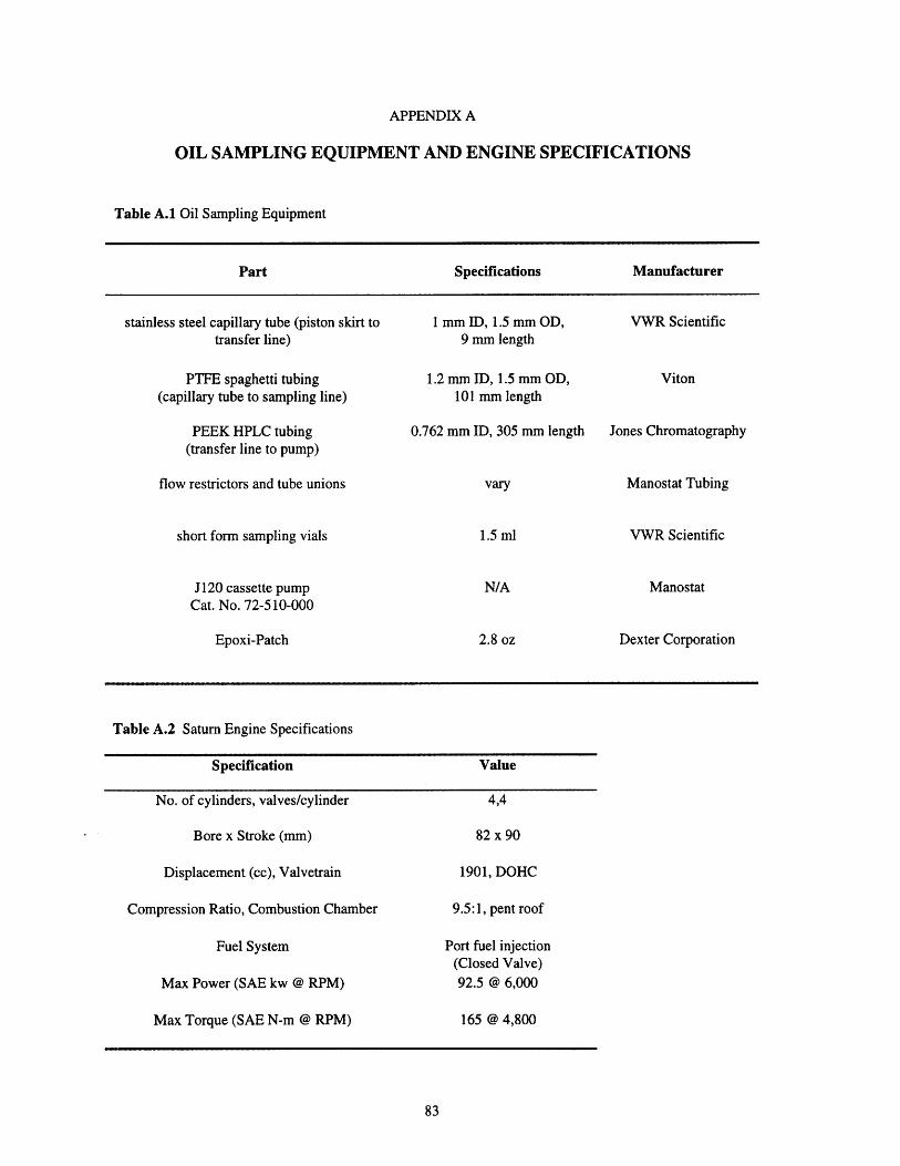
APPENDIX A
OIL SAMPLING EQUIPMENT AND ENGINE SPECIFICATIONS
Table A.1 Oil Sampling Equipment
Part Specifications Manufacturer
stainless steel capillary tube (piston skirt to 1 mm ID, 1.5 mm OD, VWR Scientifictransfer line) 9 mm length
PTFE spaghetti tubing 1.2 mm ID, 1.5 mm OD, Viton(capillary tube to sampling line) 101 mm length
PEEK HPLC tubing 0.762 mm ID, 305 mm length Jones Chromatography(transfer line to pump)
flow restrictors and tube unions vary Manostat Tubing
short form sampling vials 1.5 ml VWR Scientific
J120 cassette pump N/A ManostatCat. No. 72-510-000
Epoxi-Patch 2.8 oz Dexter Corporation
Table A.2 Saturn Engine Specifications
Specification
No. of cylinders, valves/cylinder
Bore x Stroke (mm)
Displacement (cc), Valvetrain
Compression Ratio, Combustion Chamber
Fuel System
Max Power (SAE kw @ RPM)
Max Torque (SAE N-m @ RPM)
Value
4,4
82 x 90
1901, DOHC
9.5:1, pent roof
Port fuel injection(Closed Valve)92.5 @ 6,000
165 @ 4,800
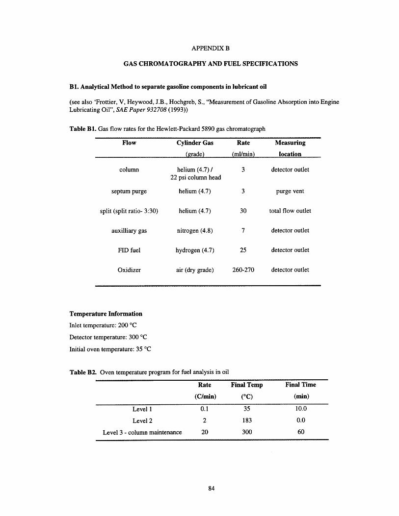
APPENDIX B
GAS CHROMATOGRAPHY AND FUEL SPECIFICATIONS
B1. Analytical Method to separate gasoline components in lubricant oil
(see also 'Frottier, V, Heywood, J.B., Hochgreb, S., "Measurement of Gasoline Absorption into EngineLubricating Oil", SAE Paper 932708 (1993))
Table B1. Gas flow rates for the Hewlett-Packard 5890 gas chromatograph
Flow Cylinder Gas Rate Measuring
(grade) (ml/min) location
column helium (4.7)/ 3 detector outlet22 psi column head
septum purge helium (4.7) 3 purge vent
split (split ratio- 3:30) helium (4.7) 30 total flow outlet
auxilliary gas nitrogen (4.8) 7 detector outlet
FID fuel hydrogen (4.7) 25 detector outlet
Oxidizer air (dry grade) 260-270 detector outlet
Temperature Information
Inlet temperature: 200 oC
Detector temperature: 300 'C
Initial oven temperature: 35 'C
Table B2. Oven temperature program for fuel analysis in oil
Rate Final Temp Final Time
(C/min) ( 0C) (min)
Level 1 0.1 35 10.0
Level 2 2 183 0.0
Level 3 - column maintenance 20 300 60
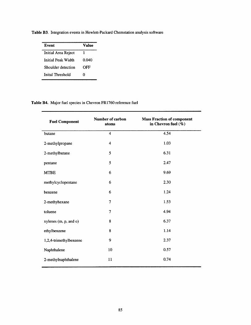
in Hewlett-Packard Chemstation analysis software
Event Value
Initial Area Reject 1
Initial Peak Width 0.040
Shoulder detection OFF
Inital Threshold 0
Table B4. Major fuel species in Chevron FR1760 reference fuel
Fuel Component
butane
2-methylpropane
2-methylbutane
pentane
MTBE
methylcyclopentane
benzene
2-methyhexane
toluene
xylenes (m, p, and o)
ethylbenzene
1,2,4-trimethylbenzene
Naphthalene
2-methylnaphthalene
Number of carbonatoms
4
4
5
5
6
6
6
7
7
8
8
9
10
11
Mass Fraction of componentin Chevron fuel (%)
4.54
1.03
6.31
2.47
9.69
2.30
1.24
1.53
4.94
6.37
1.14
2.37
0.57
0.74
Table B3. Integration events


![Wood Gas Engine Fuel[1]](https://img.pdfslide.us/doc/110x75/577d36601a28ab3a6b92e8cb/wood-gas-engine-fuel1.jpg)