The Process May Be a Complex Assembly of Phenomena

8/3/2019 The Process May Be a Complex Assembly of Phenomena

http://slidepdf.com/reader/full/the-process-may-be-a-complex-assembly-of-phenomena 1/9

Process Classification and Controller Design

The process may be a complex assembly of phenomena (or events) that relate to some

manufacturing sequence or in other words, a process is something that is to be performed in

order to achieve a certain goal. The input to the process is raw materials and energy, and

output is productive material. A simple example of process is mixing of two liquid in a tank

as shown figure 1 below.

Two liquids A and B (densities ρA and ρB respectively) are flowing in the tank at rate FA and

FB (vol/s) respectively. The compound C (density ρ) is produced inside the tank and is flow

out of the tank at a rate FC. The volume of the tank is kept constant (V) at atmospheric

temperature and pressure.

The general objectives of any industrial process are as follows:

Product quality

Production rate

Safety operation Cost effectiveness

The process control system should be designed in such a way that, it ensures product quality,

production rate, safety etc. Process control system monitor the process and also make

changes in appropriate variable of the process for the proper functioning of the process.

Control problems associated with process control system are as follows:

Process lag

Non linearity

On-line measurement

Simplicity from operator point of view

Process monitoring and diagnosis

FB, ρB

FA, ρA

FC, ρ

V ρ

Figure 1 Mixing tank



In order to design effective process control system, the behaviour and dynamics of the

process should be investigated in detail. The process may be classified as follows on the basis

of mathematical modelling.

1. First order plus dead time processes (FOPDT)

Plant, ()

, where, KP is steady state gain, L is process delay time and T is

process time constant.

FOPDT process can be further classified on the basis of delay time and process time

constant as follows.

i) The Processes whose delay time is smaller than process time constant, i.e., L ˂˂

T.

e.g., () (IEE control theory application, vol.142, No.4, july1995. By

Wang)

The close loop step response of the system is over damped.

ii) The processes whose delay time is comparable to process time constant, i.e., L ≈

T.

e.g., () (JPC vol. 20, 2010, pp.800-809)

The close loop step response is under damped.

iii) The processes whose delay time is greater than process time constant i.e., L >> T.

e.g., () (Ind. Eng. Chem. Res.1999, 38, 3007-3012)

The close loop step response is highly oscillatory and leading to instability (under

damped).

2. Second order plus dead time process (SOPDT)

Process having two poles and delay, () ,

a) When the poles are real and distinct.

Open loop step response is over damped.

Close loop step response is under damped.

e.g., () ()() [p.38,NB-03, (JPC, vol.21, 2010,pp.17-27)]

By increasing delay of the plant, close loop step response becomes oscillatory and

finally unstable.

b) When the poles are imaginary.The open loop step response is under damped.

The close loop system becomes unstable.

e.g., () [P-42, NB-3; JPC, vol, 21, 2010, pp.17-27]

Poles: -0.05±0.9987j

For a very small delay close loop step response becomes unstable.

c) When poles are real and same.

Open loop step response is over damped.

Close loop step response is under damped.

e.g., () () [P-43,NB-3; JPC, vol.21, pp.620-626].



By increasing delay time, oscillations increases and finally system becomes

unstable.

Note:- when steady state gain k P=1, roots are real, then by increasing td (to a very

high value) the close loop system becomes oscillatory but not unstable.

3.

Higher order system with delay4. Integrating system- The process having one pole at origin is called integrating

process. The step response of the process rises linearly and system is unstable.

e.g., () ()()

The close loop step response is underdamped. By increasing delay time, oscillations

increases and finally system becomes unstable.

5. Non-minimum phase system

The system, having zero in the right half of s-plane is called non-minimum phase

system.

e.g., () () [p-51, NB-3, JPC, Vol.20, 2010, pp-800-809]

The poles of the system are complex. Open loop step response is under damped and

the output initially goes opposite to the steady state value. The close loop step

response is unstable. The instability of unity negative output feedback close loop

system is due to imaginary poles and not because of right half plane zero. Consider

another example, () () , the open loop poles are real, open loop step

response is over damped. The close loop step response of the system is under damped.

The control techniques applied in the industrial process are as follows:

On-off controller

Lag-lead controller

PID controller

On-off controller or two-position controller is one of the simplest and most adopted

industrial controllers. When the error signal is positive, (i.e., the controlled variable is below

the set point value) the controller output is set to maximum and when the error signal is

negative, the controller output is set to a minimum value. The on-off controller operates in

two modes, either a minimum or maximum value. The mathematical equation describing the

characteristic of on-off controller is as follows:

{ (1)

The drawback associated with on-off controller is persistent oscillation of the controlled

variable about the set point and wear and tear of actuating device.



To overcome the drawback of on-off controller, a dead zone or hysteresis is employed. The

dead zone or neutral zone is the range of error in which controller takes no action as shown in

figure 3.

In hysteresis the controller output is different for same value of error, which depends on the

path of the error as shown in figure 4. As the error increases from negative to positive value,

it follows a different path from the path of the controller output when error decreases from

positive to negative value.

Thus, by increasing neutral zone and area of the hysteresis loop, the period of the oscillationwill be increased.

umin

umax

u

-e e

Dead zone

umin

umax

u

-e e

Dead zone

umin

umax

u

-e e

Figure 2 Ideal on-off controller

Figure 3 On-off controller with dead zone

Figure 4 on-off controller with hysteresis.



Since, oscillation is the in built nature of the on-off controller; it is applied to the slow

processes like, heating of space, liquid, filling of the huge tank etc.

PID controllers

The PID controller is very popular and easily implementable industrial controller. The

parallel form of PID controller is,()

( )

Where KP is proportional gain constant, KI is integral gain constant and KD is derivative gain

constant.

PID controller implemented in series form is as:

() ( )( )

Where

A PID controller may be considered as an extreme form of a phase lead-lag compensator with

one pole at the origin and the other at infinity. Similarly, its cousins, the PI and the PD

controllers, can also be regarded as extreme forms of phase-lag and phase-lead compensators,

respectively. A standard PID controller is also known as the “three-term” controller .

The “three-term” functionalities are highlighted by the following.

The proportional term — providing an overall control action proportional to the errorsignal through the all-pass gain factor.

The integral term — integral control overcomes the shortcomings of proportional

control by eliminating offset without the use of excessive large controller gain. Itreduces steady-state errors through low-frequency compensation by an integrator.

The derivative term — derivative control uses the rate of change of error signal and it

improves transient response through high-frequency compensation by a differentiator.

The individual effects of these three terms on the closed-loop performance are summarized in

Table I. Note that this table serves as a first guide for stable open-loop plants only.

Closed-loop

response

Rise time Overshoot Settling time Steady state

error

Stability

Increasing KP Decrease Increase Small

increase

Decrease Degrade

Increasing KI Small

decrease

Increase Increase Large

decrease

Degrade

Increasing

KD

Small

decrease

Decrease Decrease Minor

change

Improve

Table 1 Effects of independent P, I, and D tuning

[K H Ang]

The stability improvement using derivative control can’t be generalised, since derivative can

degrade stability for a system having transport delay, such problem regarding tuning of

derivative term make many control person to switch off the derivative term. But for optimumperformance Kp, Ki and Kd are mutually dependent in tuning.



The series structure

A PID controller may also be implemented in series form in which PD and PI controller are

cascaded, if both zeros are real i.e.

Where

EFFECT OF INTEGRATOR TERM

Destabilising effect of the integral termIf integral action is implemented with proportional control then transfer function of PI will be

( ) , gain will be increased by a factor of

. (5)

And simultaneously increase the phase lag of the system by

Hence by adding integral term both phase margin (PM) and gain margin (GM) are reduced

and the close system becomes oscillatory and potentially unstable.

The derivative term

Stabilising and destabilising effect of derivative term

The derivative term provide phase lead to the system and so reduces the phase lag caused by

integrator term, in this way it improve stability. This action is also helpful in hastening loop

recovery from disturbances. However, the derivative term is often misunderstood and

misused. For example, it has been widely perceived in the control community that the

derivative term improves transient performance and stability. But this perception is notalways valid. To see this, note that adding a derivative term to a pure proportional term

reduces the phase lag by

Which tends to increase the phase margin, at the same time gain is increased by a factor of

And hence the stability may be increased or decreased because phase margin is increased but

gain margin is reduced.



To prove that adding a differentiator could actually destabilise the closed-loop system,

consider without loss of generality a common first-order lag plus delay plant as described by

where is the process gain K; is the process time-constant T; and L is the process dead-time or

transport delay. Suppose that it is controlled by a proportional controller with gain and now a

derivative term is added. This results in a combined PD controller as given by

The overall open-loop feedforward-path transfer function becomes

with gain becoming

where the inequality has been obtained because

√ (

)(

)is monotonic with

. This implies that the gain is not less than 0 dB if and or and and

In these cases, the 0 dB gain crossover frequency is at infinite, where the phase

Hence, by Bode or Nyquist criterion, there exist no stability margins and the closed-loop

system will be unstable.

Lead – lag controller

Consider the compensator with the transfer function as() () .

When || ||, the controller is called phase lead controller.

The pole-zero plot of phase lead controller is shown in figure

below.

When

|

|

|

|, the controller is called phase lag controller.



Controller design methods

1. Pole placement

2. Pole-zero placement

3.

Partial pole placement(Dominant pole placement)4. Z-N tuning

Z-N tuning

There are two method of Z-N tuning

1. Step response method

2. Frequency response method

And in every method there are two steps,

Process identification

Controller parameter selection

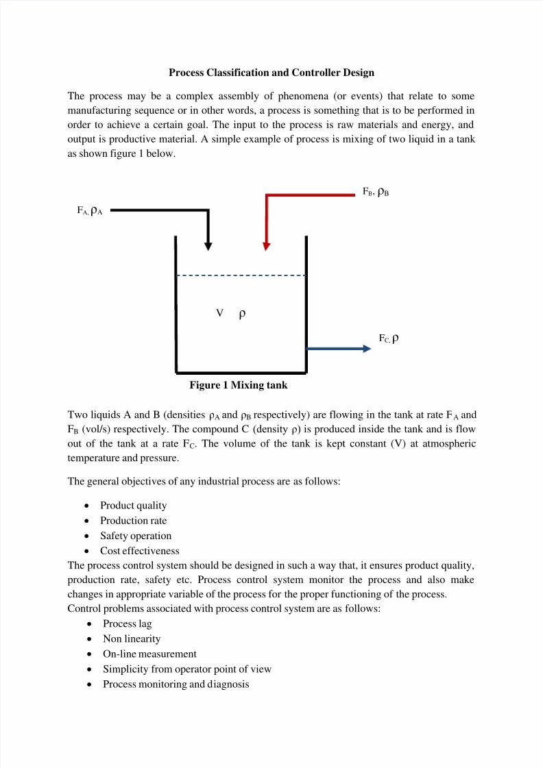
1. Step response method: - This is also called first method or open loop method. This

method is based on the step response of the plant. Two parameters are determined by step

response of open loop system. The point where, the slop of step response is maximum is

determined and the tangent at this point is drawn. The intersection of the tangent and the

axes gives the value of and . The model is characterized by and . The model

corresponds to integrator plus delay. The design criteria is quarter amplitude decay ratio.

The PID parameter as a function of and is given in table below.

Controller K Ti Td Tp

P ⁄

PI ⁄

PID ⁄

2. Frequency response method: - This method is also called second method or close loop

method.

Am litude

Tangent

Time

Figure 5 categorization of step response in Z-N step response

method



Documents

The Process May Be a Complex Assembly of Phenomena