1

The Problem of Scheduling Technicians andInterventions in a Telecommunications Company

Sérgio Garcia Panzo Dongala

November 2008

Abstract

In 2007 the challenge organized by the French Society of Operational Research and Decision

Analysis, known as ROADEF’s 2007 Challenge, consisted of solving an optimization problem

proposed by France Telecom. The main goal of this problem is to schedule technicians and

interventions in such way that the interventions stop in the lowest possible time, by taking into

account a set of precedence constraints, technician’s availability, and other constraints. On the

other hand, for each instance, a budget is given that represents the amount of money available

to outsource interventions. In this thesis, we propose several algorithms for tackling this

problem. We started by formalizing it as an integer programming problem. However, the

experimental results obtained for large size instances indicate that such an approach may have

computational limitations. Therefore, we also present an experimental analysis on the

performance of some heuristics, such as local search and simulated annealing, which return an

approximation of the optimum in a reasonable amount of time. Some of these heuristics were

able to reach similar results to those obtained by more complex and high performing algorithms

for the final phase of the ROADEF challenge.

Keywords: Combinatorial Optimization, Technicians and Interventions Scheduling.

2

1. Introduction

The goal of this paper is to study solution methods to solve an optimization problemproposed by France Telecom in the ROADEF Challenge 2007. France Telecom is a large company of telecommunications services that owned most of the marketshare in France. With the strong development of broadband internet (ADSL) and related services, the number of interventions is steadily increasing. Due to the end of telecommunication monopoly, the company had to be even more competitive in this increasing market and had to cut off the increasing need for technicians. To achieve this goal, the company wanted to introduce some improvements in the process of scheduling technicians and interventions.

An intervention consists on the resolution of a problem detected in the telecommunications network. Usually, these problems are not solved immediately. Its resolution must be scheduled according to a plan that prioritizes most critical interventions. Currently, the schedules are created on a daily basis, where each group has a supervisor that assigns technicians to interventions. These schedules are based on the formal description of the interventions and the technicians’ skills. Each Intervention needs a minimum number of technicians with certain skillsand some of these interventions have precedence constraints. On the other hand,the technicians are not available every day and there is budget available for outsourcing. This assignment takes also into account a lot of parameters that are difficult to integrate into a modeling system, such as personal affinity between technicians, tutoring, and very specific knowledge of the Intervention or geographical information (for example, where the technician lives).

Recognizing that schedules made this wayhardly guarantees good results, the company intends to use an algorithm that guarantees better scheduling (with lesser ending times of interventions). The aim of

this challenge is to provide efficient schedules that will provide a first sketch tothe supervisor.In this paper, the problem was formalized in terms of integer linear programming and solved using an exact method available in the software package GAMS. The experimental results demonstrate that this approach is only able to solve small instances. In order to solve largerinstances, we propose and test several heuristics that obtain a good approximationof the optimum in little computational time. The results obtained by some of these heuristics are reasonably good. Indeed, the results obtained were good enough to beaccepted for the final phase of the challenge.

2. Concepts Definition

In the following subsections we cover some important concepts related to Combinatorial Optimization.

2.1 Combinatorial Optimization Problems.In Combinatorial Optimization Problem(COP), one is concerned on finding the best among many possible solutions according to a given cost function. Many practical problems can be formulated as COPs. Theexpression combinatorial is related to the fact that exist only a finite number of possible solutions, and that any solution of the problem has a combinatorial property: it can be a permutation, an arrangement, a partition of items, a subset that corresponds to the a selection of a set of items or a tree or graph which indicates the relationshipbetween items (Papadimitiou & Steiglitz, 1982). In Computer Science, a COP is formally described as (Garey and Johnson, 1979):

a set of instances;

for each instance, a set S of feasible solutions (or just feasible set); and

an objective function f which assigns to each instance and each

3

feasible solution, an objective function value.

The versatility of the COPs stems from the fact that, in many practical problems, activities and resources, such as machines, airplanes and people, are indivisible (this way we see the integrality condition). Also, many problems have only a finite number of alternative choices and consequently can appropriately be formulated as COP. Such problems occur in almost all fields of management (e.g. finance, marketing, production, scheduling, inventory control, facility location and layout, data-base management), as well as in many engineering disciplines, e.g. optimal design of waterways or bridges, circuitry design and testing, the layout of circuits to minimize the area dedicated to wires, design and analysis of data networks, energy resource-planning models, logistics of electrical power generation and transport(Grötschel, 1992).

We will now describe some classical COP to provide both an overview of the diversity and versatility of this field and to show that the solution of large real-world instances of such problems requires the solution method to exploit the specialized mathematical structure of the specific application. The following examples are related to the problem to be tackled in this paper:

Knapsack problems: This problem arises when one wants to fill a knapsack that can hold a total weight of W with a subset of items from a list of n possible items each with weight and value so that the total

value of the items packed into the knapsack is maximized.

Network and graph problems: Many optimization problems can be represented by a network, where a network (or graph) is defined by nodes and by arcs connecting those nodes. Many practical problems arise in physical networks such as city streets, highways, rail systems, communication networks, and integrated circuits. In addition, there are many problems which can be modeled as networks even when there is no underlying physical network. For

example, one can think of the assignment problem where one wishes to assign a set of persons to some set of jobs in a way that the cost of the assignment is minimized. In this case, one set of nodes represents the people to be assigned, another set of nodes represents the possible jobs, and an arc connects a person to a job if that person is able to perform that job.

3. The Problem of Scheduling Technicians and Interventions in a TelecommunicationsCompany

In this section, we explain the Problem ofScheduling Technicians and Interventionsfor a Telecommunications Company (which we abbreviate as PSTITC) in more detail. Firstly, we show how the company performsthe scheduling. Then, we present the intended modifications and the goals required by France Telecom.

3.1 Problem Overview

As we can observe in Figure 1, when problems are detected in the telecommunications network (represented in the figure by light blue squares enumerated from 1 to 8 in the left upperpart) they are processed by a technicianchief (represented by the blue dark

Figure 1-Division Organization

4

rectangle). This person groups interventions and distributes them to the different groups of technicians in the next level (represented by the light blue rectangles); for example, four interventions (from 1 to 4) were sent to group A on the left side. Each group has one technician chief (represented in green) that decides which interventions that must be planned and which must not be planned (thus, they are sent for outsourcing). For example, the supervisor of group A decides to send Intervention 1 for outsourcing whereasinterventions 2, 3 and 4 are planned. This decision is made by taking into account the budget for outsourcing that is established for the group. On the other hand, the supervisor also creates teams (represented by yellow rectangles) to solve interventions (interventions 2, 3 and 4). The decisions taken by a group supervisor form an instance of the PSTITC (represented by the gray rectangle) that we will solve in this paper (ROADEF, 2008).

Currently, the supervisor takes also into account a lot of parameters that are difficult to integrate into the modeling system, such as personal affinity between technicians, tutoring and very specific knowledge of the Intervention or geographical information.Clearly, this strategy cannot guarantee ascheduling close to the optimum. This results in delays of interventions ending times that lead to increase for the need of more technicians and, finally, it meanshigher costs.

The France Telecom wants an algorithm that creates better scheduling on an automated way. The final algorithm willprovide the optimum value, or an approximation, to the supervisor. Based on the returned solution, he will make the minimum possible changes in order to guarantee that interventions are finished in a time as close as possible to the value obtained by the algorithm.

3.2 The Outsourcing Problem

The PSTITC is divided into three sub-problems: The selection of interventions to be outsourced, the problem of schedulingtechnicians and the problem of scheduling interventions.

In the first step in the resolution of the PSTITC we will have to decide whichinterventions must be outsourced, we decide it because this part of the problem is the most ease to solve. We introduce now some proprieties of the interventions that are needed to understand the procedure:

Priorities: There are four levels of priorities. These characterize the urgency of the interventions. An Intervention with priority one is more urgent than another one with priority two.

Precedence: Some interventions can only initiate after others had finish.

Cost: For each Intervention, there is a cost for outsourcing, whichrepresents the monetary valuepaid to the contracted company.

Time: Each Intervention has a timeassociated with its execution.

For each instance of the problem there exists an outsourcing limit. In any scheduling the total cost of interventions outsourced can not exceed this limit. Another constraint of this problem is the fact that, if one Intervention is executed by outsourcing then all its successors must also be done by outsourcing.

The problem of deciding whichinterventions must be sent for outsourcing is related with the knapsack problem in the following way: The items are the interventions, the weight of each items are the cost of outsourcing, the limit of the knapsack is the limit for outsourcing, the value of the item is the result of the ratio(time/cost), and the decision of placing anitem in the knapsack is symbolized by the decision of sending an Intervention foroutsourcing. Although it may look simple

5

this part of the problem itself is a NP-Hard problem, and what makes it difficult to solve it is the precedence constraint (Hashimoto et al, 2007).

3.3 Technicians and InterventionsScheduling The two following sub-problems(technicians and interventions scheduling) are solved altogether. We now present some characteristics of interventions and technicians that are related to these two problems:

The technicians’ skills are classified according to domains. Each domain is divided into levels. For each instance there is a number of domains and a level number.

An Intervention needs a minimum number of technicians with certainskills.

Some technicians are not available in certain days, due to vacation, illness, formation, and so on.

Two interventions performed at the same day and by the same teamare executed in different times. One team does not work on more than one Intervention at the same time.Thus, one Intervention only willstart after the end of the other.

The interventions are performed in different locations and the teamsshare the available cars (that are of limited number). Therefore, the members of the same team are always together. This implies that the composition of technicians of one team in one day does not change during that day.

The required number of technicians at a given level for an Intervention is cumulative since a technician of a given level is also qualified for all the smaller levels of the same competence domain. For example, if a technician has the capacity of working on interventions with level three, he can also work on interventions requiring only a skill level of two or one.

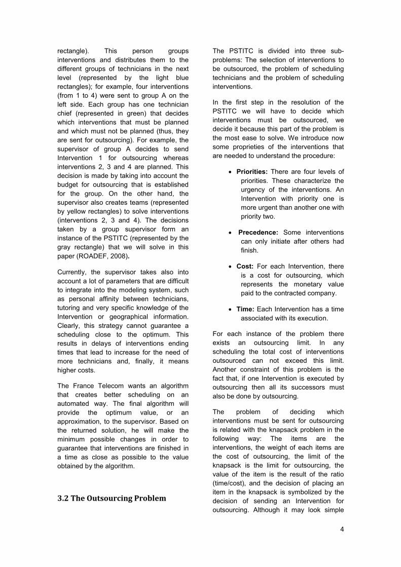
The assignment of technicians and interventions presented in this section can be seen as two connected problems: On one hand, one must create teams of technicians for each day, where each teammust have at least one technician. On the other hand one must assign the interventions to teams while fulfilling theconstraints presented above. This way, the PSTITC can be seen as set of three problems, as we can see in next figure.

Figure 2-Overview of the PSTITC

The objective function according to the statement of ROADEF is (ROADEF, 2008):

Min

Where:

: Is the ending time of the last

scheduled Intervention of priority one.

: Is the ending time of the last

scheduled Intervention of priority two.

: Is the ending time of the last

scheduled Intervention of prioritythree.

: Is the ending time of the last

scheduled Intervention.

PSTIT

6

4. Solving the Roadef’2007 Challenge

In this section we present two ways of solving the problem described in the previous section. First we present the exact approach, which has limitations on solving instances of large dimensions. Then, forthose instances, we propose three heuristics that find an approximation of the optimum in a reasonable amount of time.

4.1 Exact approachWe developed an integer linear programming model as shown in Appendix4. We solved this model by GAMS 22.2(General Algebraic Modeling System) that is a software package that contains CPLEX11.2.1 and it uses the branch-and-bound algorithm to solve problems of integer linear programming.

Table 1 shows the results of the exact method, applied to the first five instances of the problem. We can observe that the exact approach only was able to solve the first and the second instance in 2 and 28 seconds, respectively. The red values in thecolumn time indicate that the program shown an error and it was not able to solve.

Table 1-Results of the exact approach

Given that the largest instance of the competition has 800 interventions, and the fact that in the tested instances until the moment (from 1 to 5) we do not consider the use of outsourcing (the use of outsourcing would increase the complexityof the problem) we can see that the exact method is not viable to solve this problem.

4.2 The Lower BoundBefore applying the heuristic approach, it is necessary to get a lower bound of the optimum value that would be used to evaluate the performance of the heuristic. To get this value we solved a simplified relaxed version of the original problem (Hurkens, 2007). These simplifications include the use of only one domain without levels, and do not take into account theprecedence constraints. Table 2 shows the results obtained.

Table 2-Lower bound.

4.3 Heuristic ApproachThe need for heuristic approaches ariseswhen the exact method is not able to solvelarge realistic instances. In this section we present some heuristics to solve this problem.

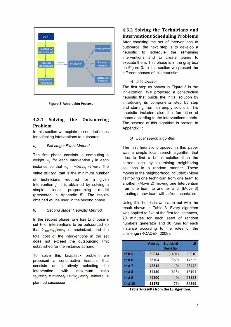
As seen in Section 3, the PSTITC is divided in 3 sub-problems: Choosing interventions to outsource, formatting teams and assigning interventions to teams (see Figure 2). The problem of outsourcing will be the first to be solved; this process involves the use of an exact method followed by a heuristic that decides whichinterventions must be sent for outsourcing. This process is shown in the part detached in yellow in Figure 3.

Inst Int GAP rel

GAP Abs

Results Time

1 5 0,064 150 2340 2s2 5 0 0 4755 28s3 20 - 39:23s4 20 - 2:52:51s5 50 - 55s

7

Figure 3-Resolution Process

4.3.1 Solving the Outsourcing ProblemIn this section we explain the needed steps for selecting interventions to outsource.

a) Fist stage: Exact Method.

The first phase consists in computing a weight for each Intervention j in each

instance so that . The

value that is the minimum number

of technicians required for a given Intervention j, it is obtained by solving a simple linear programming model (presented in Appendix 5). The results obtained will be used in the second phase.

b) Second stage: Heuristic Method.

In the second phase, one has to choose a set H of interventions to be outsourced so that is maximized, and the

total cost of the interventions in the set does not exceed the outsourcing limit established for the instance at hand.

To solve this knapsack problem we proposed a constructive heuristic that consists on iteratively selecting the Intervention with maximum ratio

without a

planned successor.

4.3.2 Solving the Technicians and Interventions Scheduling ProblemsAfter choosing the set of interventions to outsource, the next step is to develop a heuristic to schedule the remaining interventions and to create teams to execute them. This phase is in the gray box on Figure 3. In this section we present the different phases of this heuristic:

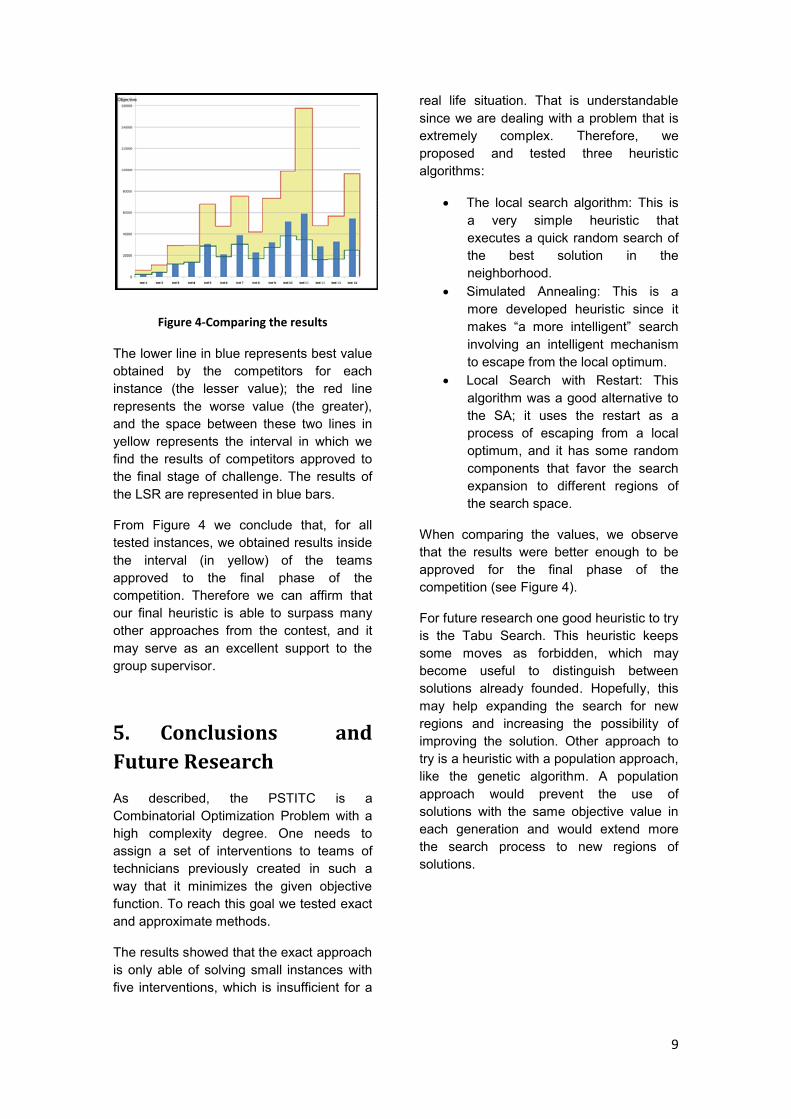
a) InitializationThe first step as shown in Figure 3 is the initialization. We proposed a constructive heuristic that builds the initial solution by introducing its components step by stepand starting from an empty solution. This heuristic includes also the formation of teams according to the interventions needs. The scheme of this algorithm is present in Appendix 1:

b) Local search algorithm

The first heuristic proposed in this paperwas a simple local search algorithm thattries to find a better solution than the current one by examining neighboring solutions in a random manner. Thesemoves in the neighborhood included: (Move 1) moving one technician from one team to another; (Move 2) moving one Interventionfrom one team to another and, (Move 3) creating a new team with a free technician.

Using this heuristic we came out with theresult shown in Table 3. Every algorithm was applied to five of the first ten instances, 20 minutes for each seed of random numbers generator and 30 runs for each instance according to the rules of the challenge (ROADEF, 2008).

Averag Standard Deviatio

LB

Inst 5 39014 (1401) 26910

Inst 6 28704 (369) 17625

Inst 7 46815 (0) 28442

Inst 8 34550 (613) 16191

Inst 9 49200 (0) 25553

Inst 10 59575 (76) 36399Table 3-Results from the LS algorithm.

8

As we can see on the Table 3 the results are far away from the lower bound in the last column (obtained in section 4.2). Therefore, we tested other two heuristics.

c) Simulated Annealing

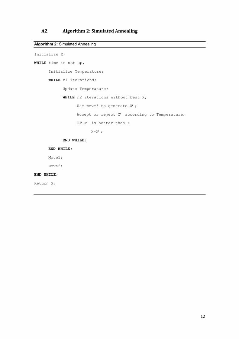
One of the difficulties in designing a local search heuristic is to arrange an effectiveway of escaping local optima. The second heuristic proposed is the Simulated Annealing (SA), which uses a process to escape the local optimum. The scheme that resumes the main steps of this algorithm is shown in Appendix 2.

The following table presents the results obtained with Simulated Annealing.

SA SD LS L B

Inst 5 41280 (0) 36240 26910Inst 6 31680 (0) 27990 17625Inst 7 45396,1 (460) 46815 28442Inst 8 35280 (0) 33180 16191Inst 9 48900 (0) 49200 25553Inst 10 56784,3 (0) 59295 36399

Table 4-Results of SA

According to Table 4, we can observe that SA (first column) obtained some better results on larger instances that the previous heuristic (third column). Moreover, this approach also obtained lower standarddeviations (second column). However, the results are still worse for instances 5, 6 and 8. Due to this inconsistency we decided to test one more heuristic.

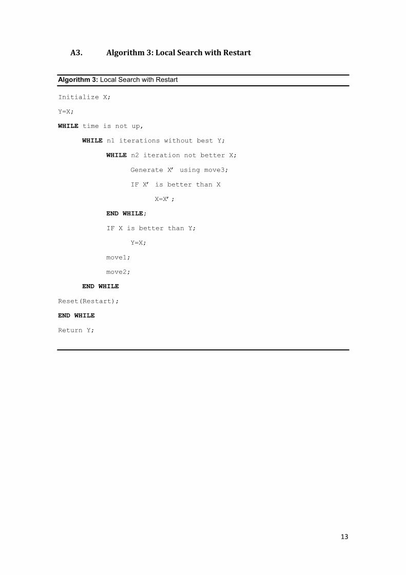
d) Local Search with Restart

A good alternative to the SA is the Local Search with Restart (LSR). In this heuristic we introduced the restart process as an alternative way to escape from the local optimum. We also added some randomness in the process. For instance, instead of introducing interventions with high priority first, we do it in a random way, so that in the restart process the solution created will not always be the same. Other change was made in the team formation

process. Instead of introducing technicians in order as they are given in the instancewe now take the decision in a randomlyway. The scheme of this algorithm is presented in Appendix 3.

We run this algorithm on five instances and we obtained the results shown in Table 5.

Number of Inter

LSR Roadef LB

Inst1 5 2340 2340 2265

Inst2 5 4755 4755 2055

Inst3 20 13068,4 11880 11310

Inst4 20 13620 13452 10629

Inst5 50 31236,1 28845 26910

Inst6 50 21576,6 18795 17625

Inst7 100 40116,7 30540 28442

Inst8 100 23115,5 16920 16191

Inst9 100 34056,3 27692 25553

Inst10 100 52348,7 38296 36399

Inst11 200 58968,3 34395 32085

Inst12 300 28989,1 15870 141296

Inst13 400 34368,3 16020 14610

Inst14 400 56382,1 25305 16635

Table 5-Result of the LSR

The results in Table 5 clearly show thatLSR (second column) is better than the other two local search heuristics in both smaller and larger instances. This table indicates that for instances with less than 20 interventions (one to four) we obtained the best value found (third column). However, looking to first column (number of interventions), we see that the algorithm performance deteriorates with the increase on instance size.

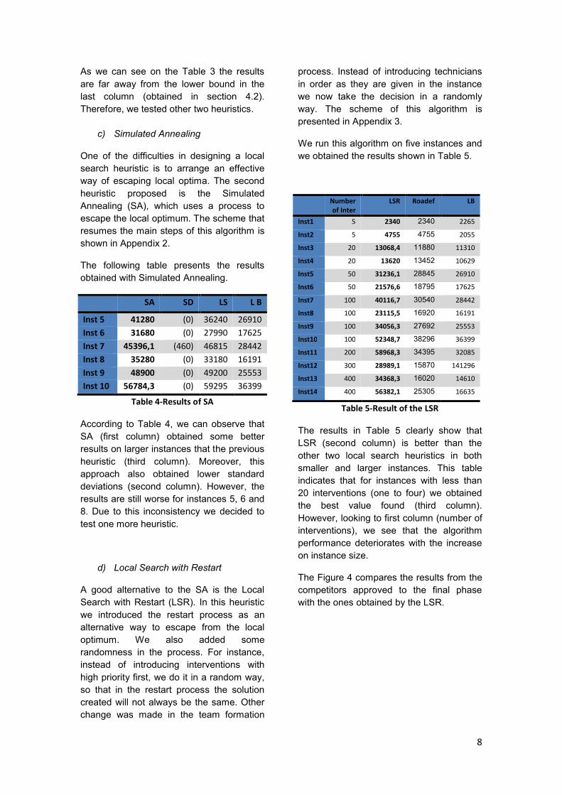
The Figure 4 compares the results from thecompetitors approved to the final phase with the ones obtained by the LSR.

9

Figure 4-Comparing the results

The lower line in blue represents best value obtained by the competitors for each instance (the lesser value); the red line represents the worse value (the greater), and the space between these two lines in yellow represents the interval in which we find the results of competitors approved to the final stage of challenge. The results of the LSR are represented in blue bars.

From Figure 4 we conclude that, for all tested instances, we obtained results inside the interval (in yellow) of the teams approved to the final phase of the competition. Therefore we can affirm that our final heuristic is able to surpass many other approaches from the contest, and it may serve as an excellent support to the group supervisor.

5. Conclusions and Future Research

As described, the PSTITC is a Combinatorial Optimization Problem with a high complexity degree. One needs to assign a set of interventions to teams of technicians previously created in such a way that it minimizes the given objectivefunction. To reach this goal we tested exact and approximate methods.

The results showed that the exact approachis only able of solving small instances with five interventions, which is insufficient for a

real life situation. That is understandable since we are dealing with a problem that is extremely complex. Therefore, we proposed and tested three heuristic algorithms:

The local search algorithm: This is a very simple heuristic that executes a quick random search of the best solution in the neighborhood.

Simulated Annealing: This is a more developed heuristic since it makes “a more intelligent” search involving an intelligent mechanism to escape from the local optimum.

Local Search with Restart: This algorithm was a good alternative tothe SA; it uses the restart as a process of escaping from a local optimum, and it has some random components that favor the search expansion to different regions of the search space.

When comparing the values, we observe that the results were better enough to be approved for the final phase of the competition (see Figure 4).

For future research one good heuristic to try is the Tabu Search. This heuristic keepssome moves as forbidden, which maybecome useful to distinguish betweensolutions already founded. Hopefully, this may help expanding the search for new regions and increasing the possibility of improving the solution. Other approach to try is a heuristic with a population approach, like the genetic algorithm. A population approach would prevent the use ofsolutions with the same objective value in each generation and would extend more the search process to new regions of solutions.

10

BibliographyGarey, M. R., & Johson, D. S. (1979). Computers and intractability - a guide to NP-completeness. San Francisco: W.H. Freeman and Company.

Grötschel, M. (1992). Discrete mathematics in manufacturing. Preprint.

Hashimoto, H., Boussier, S., & Vasquez, M. (2007). An iterated local search algorithm for technicians and interventions scheduling for telecommunications. Obtido em 20 de January de 2008, do website da Roadef 2007. http://www.g-scop.inpg.fr/ChallengeROADEF2007/ABSTRACTS/abstract_roadef01.pdf

Hurkens, C. J. (2007). Roadef. Obtido em 20 de January de 2008, de Roadef 2007: http://www.g-scop.inpg.fr/ChallengeROADEF2007/TEAMS/roadef44/abstract_roadef44.pdf

Papadimition, H. C., & Steiglitz, K. (1982). Combinatorial Optimization: Algorithms and Complexity. Dover Publications.

ROADEF. (2008). ROADEF. Obtido em 17 de agosto de 2008, de ROADEF.ORG: http://challenge.roadef.org/2009/index.en.htm

11

6. Appendixes

A1. Algorithm 1: Initialization

Algorithm 1: Initialization

Start

Cost =0,

FOR All priorities k from 1 to 4,

WHILE Exist interventions with priority k

Choose the next Intervention i with the biggest requirement;

IF i has precedent;

Introduce all precedents;

Introduce i;

END WHILE;

END FOR;

12

A2. Algorithm 2: Simulated Annealing

Algorithm 2: Simulated Annealing

Initialize X;

WHILE time is not up,

Initialize Temperature;

WHILE n1 iterations;

Update Temperature;

WHILE n2 iterations without best X;

Use move3 to generate X’;

Accept or reject X’ according to Temperature;

IF X’ is better than X

X=X’;

END WHILE;

END WHILE;

Move1;

Move2;

END WHILE;

Return X;

13

A3. Algorithm 3: Local Search with Restart

Algorithm 3: Local Search with Restart

Initialize X;

Y=X;

WHILE time is not up,

WHILE n1 iterations without best Y;

WHILE n2 iteration not better X;

Generate X’ using move3;

IF X’ is better than X

X=X’;

END WHILE;

IF X is better than Y;

Y=X;

move1;

move2;

END WHILE

Reset(Restart);

END WHILE

Return Y;

14

A4. Modeling the PSTITCIndices

: Day in which an Intervention is done (intv is the number of Intervention in

instance).

: This index if applied for teams.

: j is used to indicate Interventions, it is also used p in some restrictions.

: This index is used to indicate the position in which an Intervention is made in

a team.

: This index is used to indicate technicians. Here tec is the number of

technicians in the instance.

: This index is for domains. Here dom is the number of domains in the

instance.

: This index is used for levels. Here niv is the number of level in each domain.

: Priority of interventions. For every instance this index goes from 1 to 4.

Input data.: Array of costes for each Intervention j.

: Array of times for each Intervention j.

: Square matrix that has the value one if Intervention j has Intervention p has a

predecessor and zero if not.

: This matrix gives has the value one if the technician l is not available at day d, and zero

if is available.

This matrix has the value one is Intervention j is from priority c, and zero otherwhise.

: This is the requirement matrix that gives the number of technicians needed to

execute Intervention j on the domain m and level n.

This matrix gives the capacity of technicians. if the technician

l is capable of working with interventions on domain m and level n.

: Number of interventions of the instance.

: Number of technicians.

15

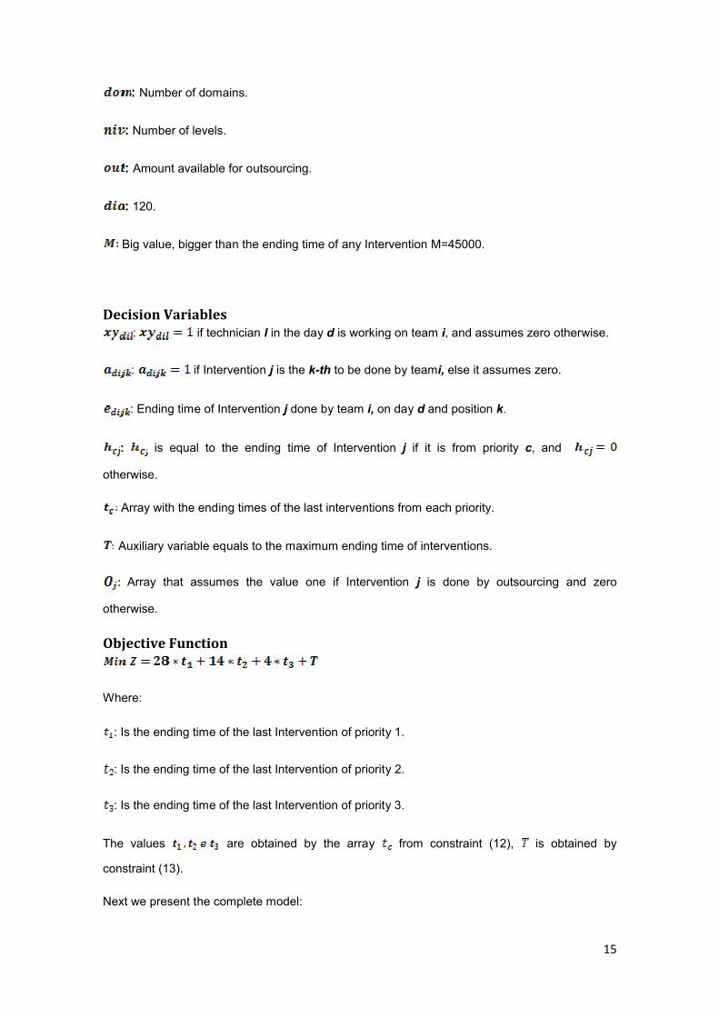
: Number of domains.

: Number of levels.

: Amount available for outsourcing.

: 120.

Big value, bigger than the ending time of any Intervention M=45000.

Decision Variables: if technician l in the day d is working on team i, and assumes zero otherwise.

: if Intervention j is the k-th to be done by teami, else it assumes zero.

: Ending time of Intervention j done by team i, on day d and position k.

: is equal to the ending time of Intervention j if it is from priority c, and

otherwise.

Array with the ending times of the last interventions from each priority.

Auxiliary variable equals to the maximum ending time of interventions.

Array that assumes the value one if Intervention j is done by outsourcing and zero

otherwise.

Objective Function

Where:

: Is the ending time of the last Intervention of priority 1.

: Is the ending time of the last Intervention of priority 2.

: Is the ending time of the last Intervention of priority 3.

The values are obtained by the array from constraint (12), is obtained by

constraint (13).

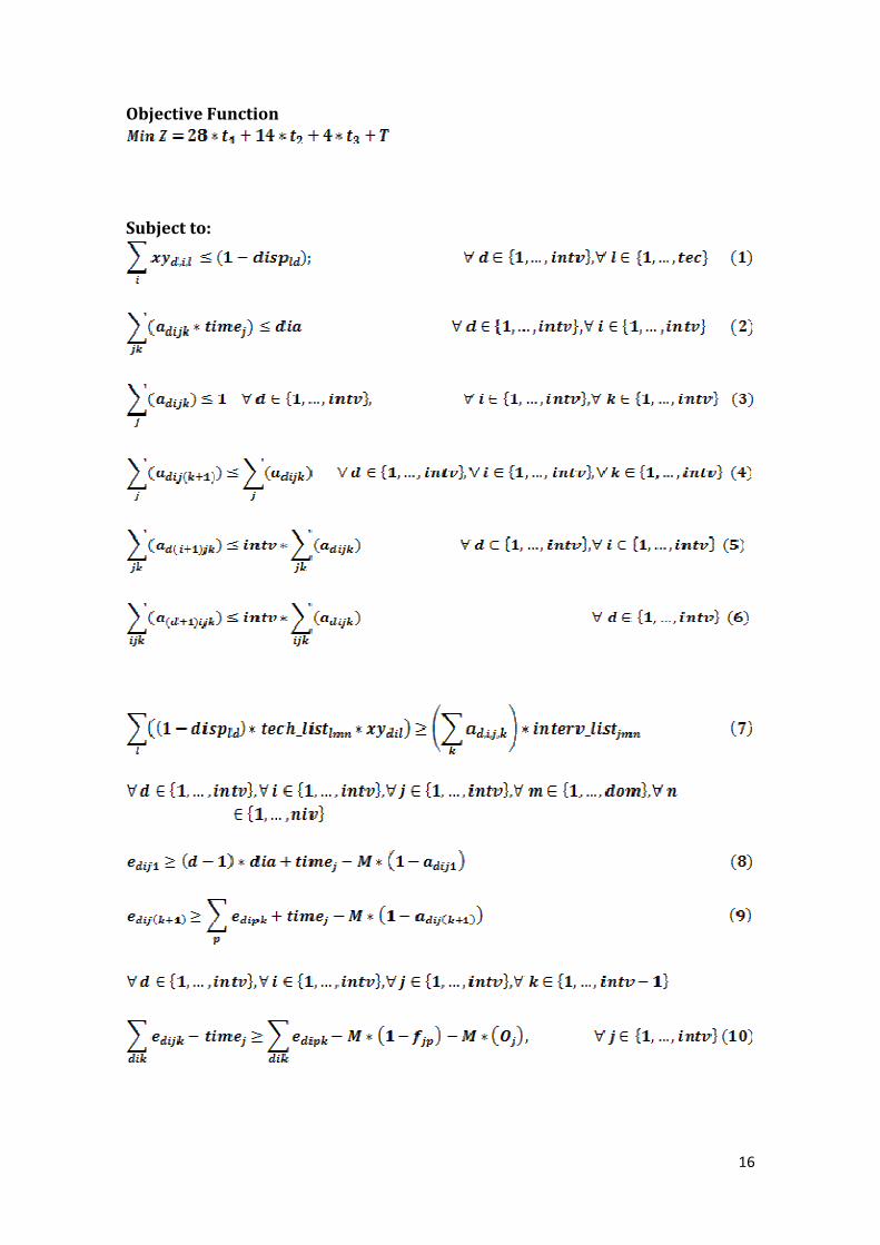
Next we present the complete model:

16

Objective Function

Subject to:

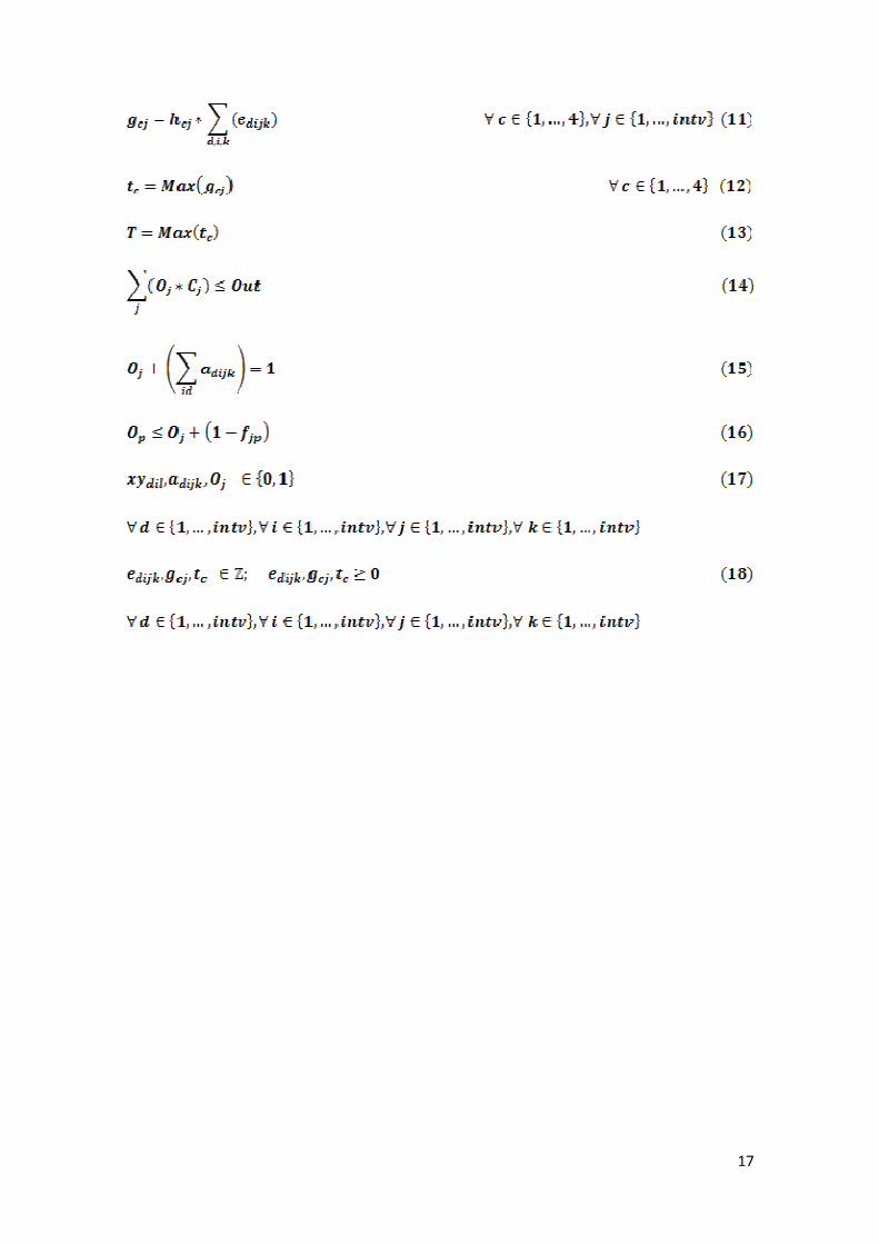
17

18

A5. Modeling the Outsourcing Problem.

Indices: j represents interventions, where intv is the number of interventions of

instances.

: Technicians, where tec is the number of technician for each instance.

: m represents the domain, where dom is the numbers of domains for the

instance.

: n represents the level, and niv is the number of levels in the instance.

Input Data: Matrix with the requirements as shwon in previous model.

Matrix with the capacities of technicians as shown in previous model.

: Number of interventions.

: Number of technicians.

: Number of domains.

: Number of levels.

: Budget for outsourcing.

Decision Variables: Number of technicians working on Intervention j.

: Assignment of technician l to Intervention j.

Objective Function

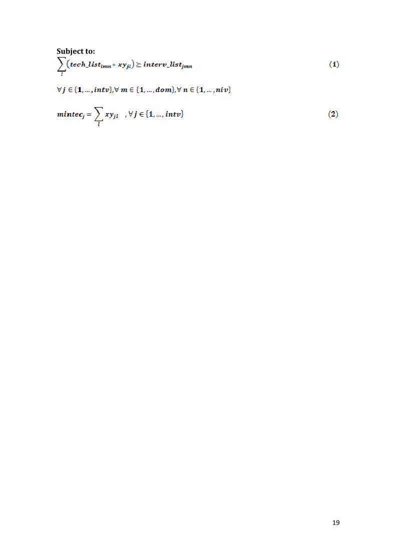
19

Subject to: