Why is ‘geography’ important?

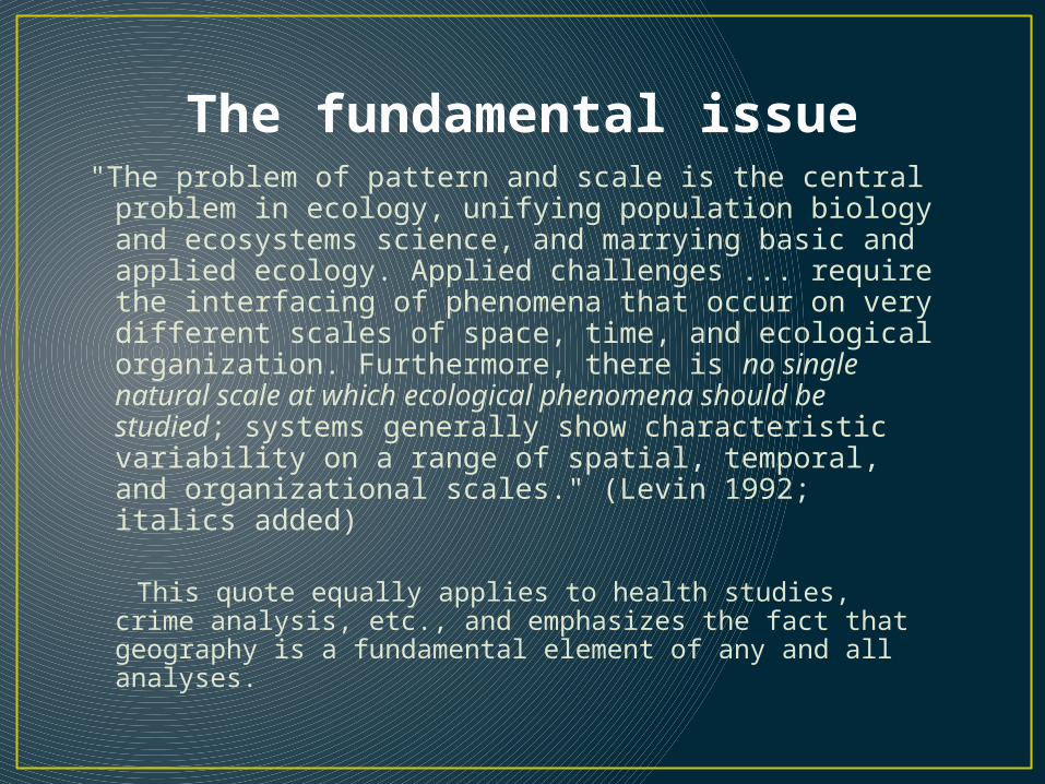
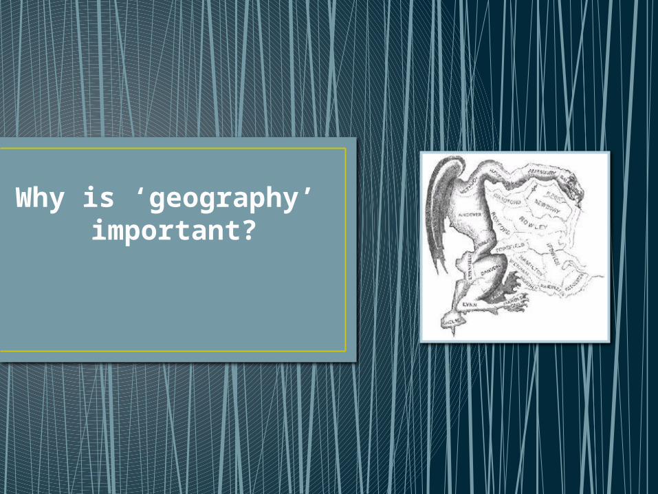
The fundamental issue"The problem of pattern and scale is the central

problem in ecology, unifying population biology and ecosystems science, and marrying basic and applied ecology. Applied challenges ... require the interfacing of phenomena that occur on very different scales of space, time, and ecological organization. Furthermore, there is no single natural scale at which ecological phenomena should be studied; systems generally show characteristic variability on a range of spatial, temporal, and organizational scales." (Levin 1992; italics added)

This quote equally applies to health studies, crime analysis, etc., and emphasizes the fact that geography is a fundamental element of any and all analyses.

A working solution• None-the-less, many have argued that

ecological phenomena tend to have characteristic spatial and temporal scales, or spatiotemporal domains (e.g., Delcourt et al. 1983, Urban et al. 1987).

• A central tenet of landscape ecology is that particular phenomena should be addressed at their characteristic scales. Likewise, if one changes the scale of reference, the phenomena of interest change.

Characteristic scales? What are some characteristic scales?

• Animals (criminals?) may select for a resource in a consistent direction or for a mixture of habitats—denoted as “simple” and “complementary” selection.

• A species that is restricted in distribution to rocky tidal zones has an obvious characteristic scale (a simple selection), while a species such as a cougar ranges widely across a broad range of habitats (a complementary selection) and, thus, identifying the appropriate scale to study cougar behaviour is much more complex.

Characteristic scales?

What are some characteristic scales?

• Similarly, serial criminals can be commuters or marauders; one commits offences primarily within their own neighbourhood (a marauder) while the other travels outside of the neighbourhood to commit their offences (a commuter). Obviously, in the one case identifying the characteristic scale of analysis is easy (i.e., the neighbourhood), while in the other a completely different scale of analysis would be required. (How to determine??)

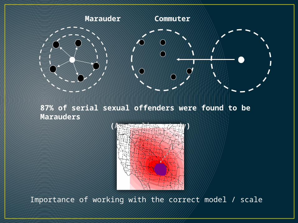
Commuter Marauder

87% of serial sexual offenders were found to be Marauders(Australian study)

Importance of working with the correct model / scale

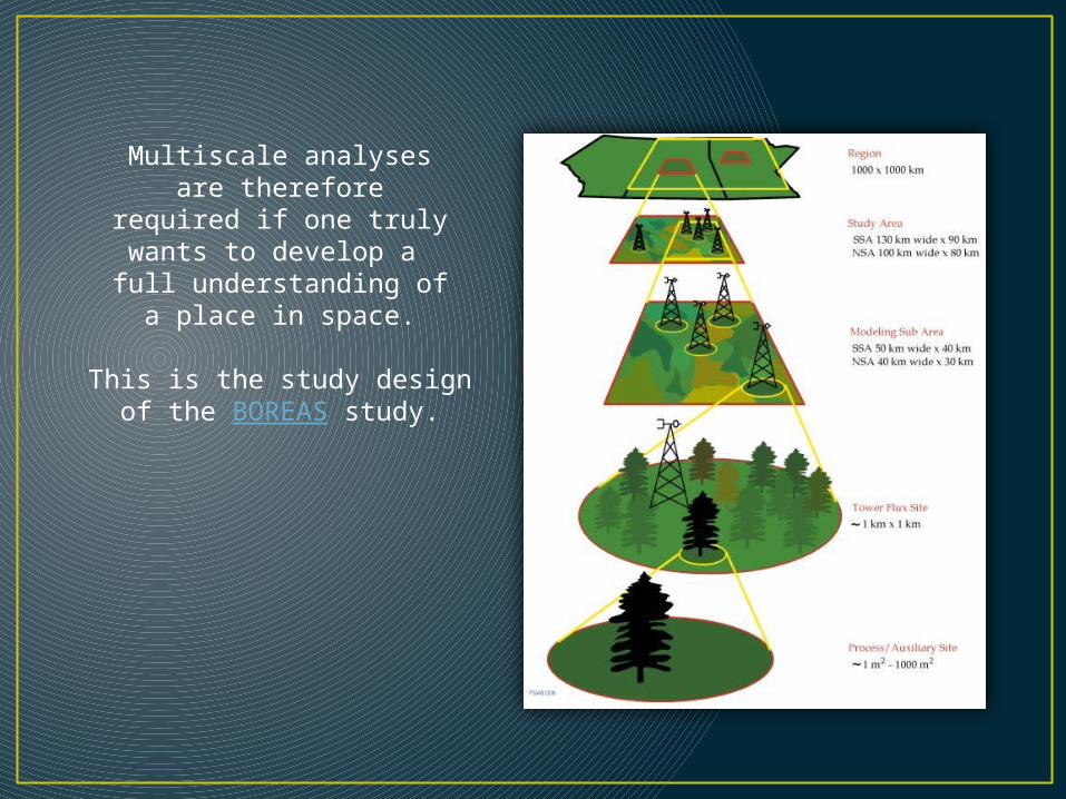
Multiscale analysesare therefore

required if one trulywants to develop a full understanding of

a place in space.

This is the study designof the BOREAS study.

Source

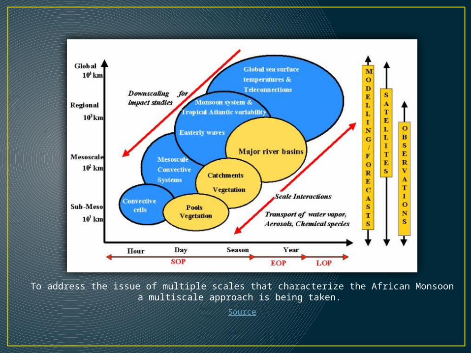
To address the issue of multiple scales that characterize the African Monsoona multiscale approach is being taken.

Why is geography important?

Issues such as:

• the scale, grain and extent of a study area,• the modifiable areal unit problem,• the nature of the boundaries of a study area,

and• spatial dependence / heterogeneity

are implicit in any spatial analysis.

Why geography is important.

• Given the above, landscape ecologists, epidemiologists, health geographers, and crime analysts all must carefully consider the 'geography' of their problem, and what effects that geography alone may have on their analyses (e.g., do more crimes occur in area A than area B simply because more people live in area A, or are there more crimes because there are higher levels of drug use in the area?).

• Simply put—are the results dependent upon the spatial nature of the data, or do they reflect the results of a process? (Most likely, a combination of both.)

Scale terminology

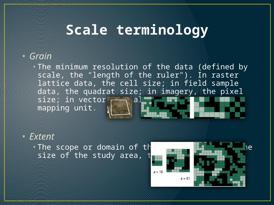
• Grain • The minimum resolution of the data (defined by scale, the

"length of the ruler"). In raster lattice data, the cell size; in field sample data, the quadrat size; in imagery, the pixel size; in vector spatial data, the minimum mapping unit.

• Extent • The scope or domain of the data (defined as the size of

the study area, typically)

Scale• "Scale" is not the same as "level of

organization." Scale refers to the spatial domain of the study, while level of organization depends on the criteria used to define the system.

• For example, population-level studies are concerned with interactions amongst conspecific individuals, while ecosystem-level studies are concerned with interactions among biotic and abiotic components of some process such as nutrient cycling.

• One could conduct either a small- or large-scale study of either population- or ecosystem-level phenomena.

Conspecific: Of or belonging to the same species

Scale• As one increases scale in a study of a

system:

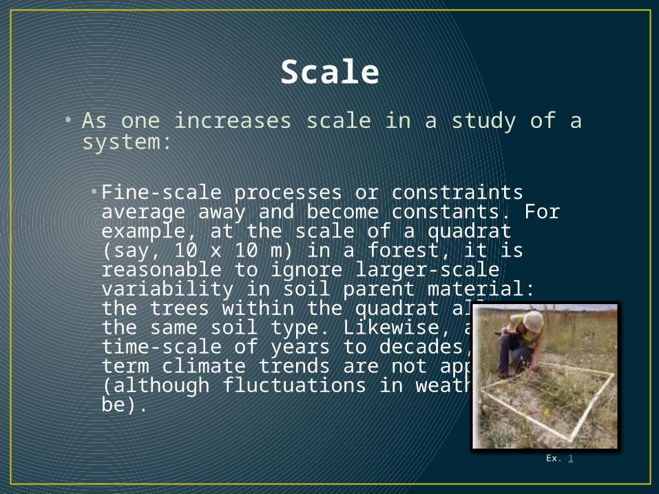
• Fine-scale processes or constraints average away and become constants. For example, at the scale of a quadrat (say, 10 x 10 m) in a forest, it is reasonable to ignore larger-scale variability in soil parent material: the trees within the quadrat all see the same soil type. Likewise, at the time-scale of years to decades, long-term climate trends are not apparent (although fluctuations in weather might be).

Ex. 1

Scale

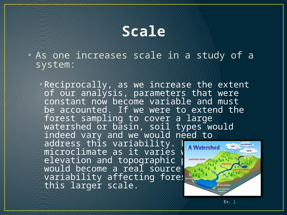
• As one increases scale in a study of a system:

• Reciprocally, as we increase the extent of our analysis, parameters that were constant now become variable and must be accounted. If we were to extend the forest sampling to cover a large watershed or basin, soil types would indeed vary and we would need to address this variability. Likewise, microclimate as it varies with elevation and topographic position would become a real source of variability affecting forest pattern at this larger scale.

Ex. 1

Scale

• Finally, new interactions may arise as one increases the extent of inquiry. At the scale of a landscape mosaic, interactions among forest stands, such as via dispersal of plant or animal species, emerge as new phenomena for study. (Emergent processes)

• The magnitude or sign of correlations may change with spatial extent. At the scale of a single habitat patch, abundances of different species might be negatively correlated due to interspecific interactions; but if one considers a set of these habitat patches in a heterogeneous landscape, any species inhabiting similar habitat types will be positively correlated.

• Thus: explanatory models are scale-dependent

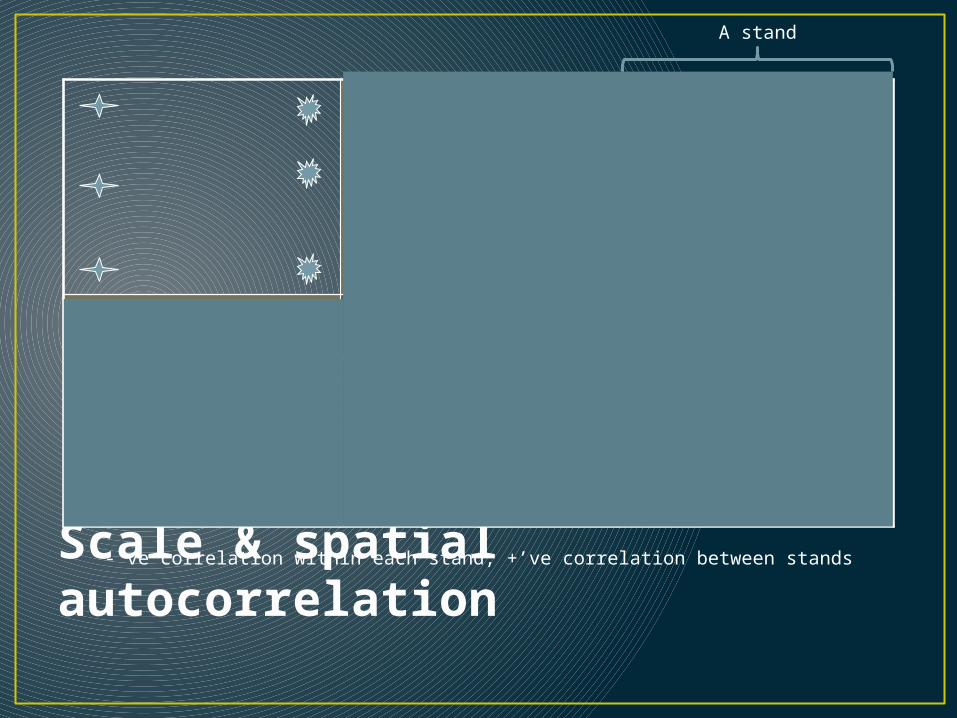
Scale & spatial autocorrelation

-’ve correlation within each stand, +’ve correlation between stands

A stand

Spatial autocorrelation

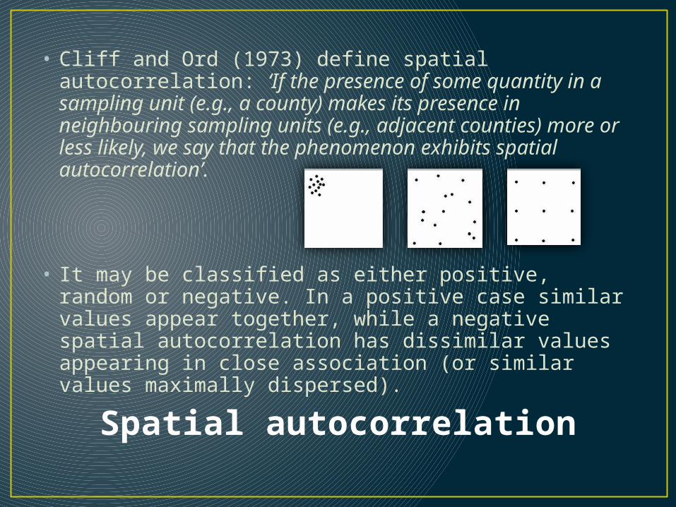
• Cliff and Ord (1973) define spatial autocorrelation: ‘If the presence of some quantity in a sampling unit (e.g., a county) makes its presence in neighbouring sampling units (e.g., adjacent counties) more or less likely, we say that the phenomenon exhibits spatial autocorrelation’.

• It may be classified as either positive, random or negative. In a positive case similar values appear together, while a negative spatial autocorrelation has dissimilar values appearing in close association (or similar values maximally dispersed).

Spatial autocorrelation• The distribution of organisms over the earths’

surface means that most ecological problems have a spatial dimension. Biological variables are spatially autocorrelated for two reasons:• inherent forces such as limited dispersal, gene flow or

clonal growth tend to make neighbours resemble each other;

• organisms may be restricted by, or may actively respond to, environmental factors such as temperature or habitat type, which themselves are spatially autocorrelated (Sokal & Thomson 1987).

• Obviously describes crime and disease patterns as well (inherent vs extrinsic forces).

Spatial autocorrelation

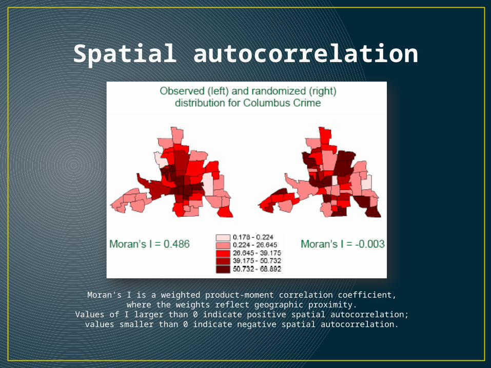
Moran's I is a weighted product-moment correlation coefficient, where the weights reflect geographic proximity.

Values of I larger than 0 indicate positive spatial autocorrelation; values smaller than 0 indicate negative spatial autocorrelation.

MAUP

• The modifiable areal unit problem is endemic to all spatially aggregated data. It consists of two interrelated parts. • First, there is uncertainty about what constitutes the objects of spatial study--identified as the scale and aggregation problem.

• Second, there are the implications this holds for the methods of analysis commonly applied to zonal data and for the continued use of a normal science paradigm which can neither cope nor admit to its existence.

Object uncertainty: Scale

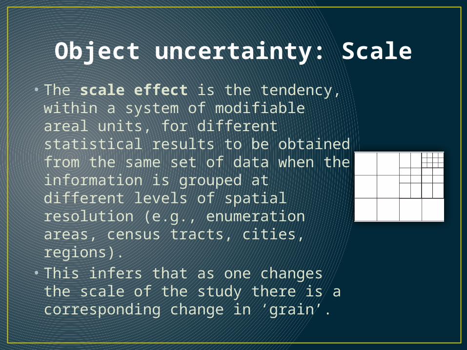
• The scale effect is the tendency, within a system of modifiable areal units, for different statistical results to be obtained from the same set of data when the information is grouped at different levels of spatial resolution (e.g., enumeration areas, census tracts, cities, regions).

• This infers that as one changes the scale of the study there is a corresponding change in ‘grain’.

Object uncertainty: Aggregation

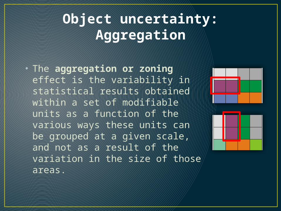
• The aggregation or zoning effect is the variability in statistical results obtained within a set of modifiable units as a function of the various ways these units can be grouped at a given scale, and not as a result of the variation in the size of those areas.

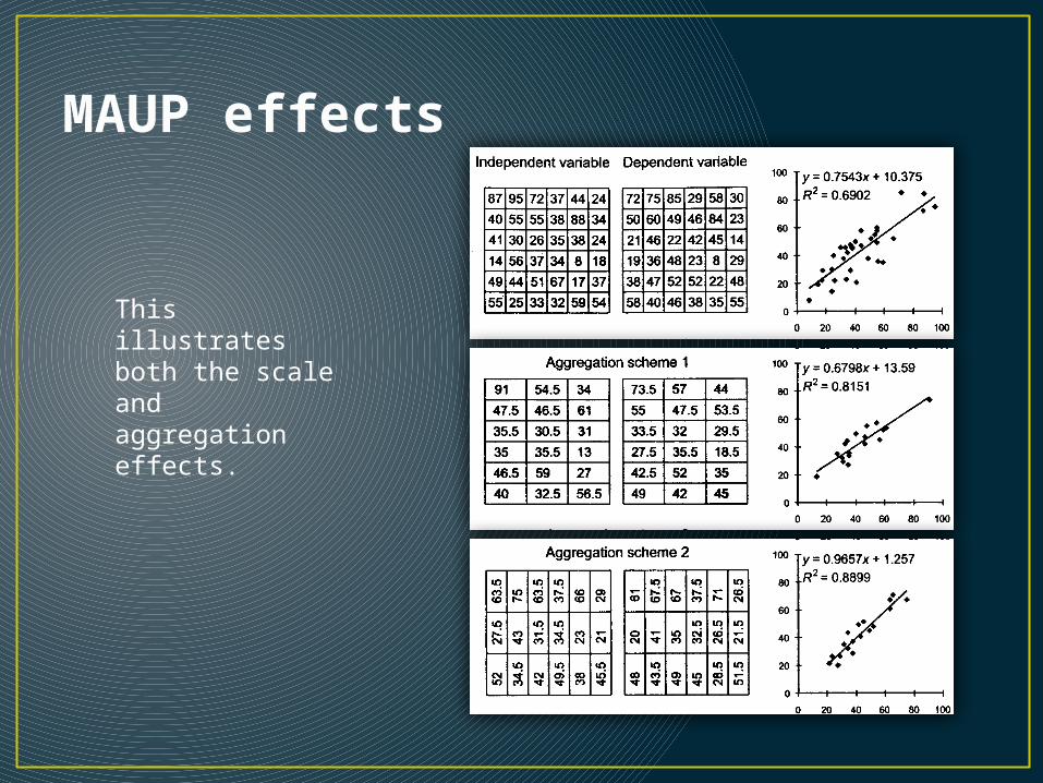
MAUP effects

This illustratesboth the scaleand aggregation effects.

Aggregation

• The problem with aggregated data comes not (only) with the data themselves or any conclusions drawn from them, but from attempts to extend the conclusions to another level of spatial resolution (usually finer, like to individual households or people). Attempting to do this is called ecological fallacy.

• All the statistics and model parameters could differ between the two levels of resolution, and we have no way to predict what they are at the finer level, given the values at the coarser level.

MAUP

• The second component of MAUP follows from the uncertainty in choosing zonal units.

• Different areal arrangements of the same data produce different results, so we cannot claim that the results of spatial studies are independent of the units being used, and the task of obtaining valid generalizations or of comparable results becomes extraordinarily difficult.

• MAUP therefore consists of two problems--one statistical and the other geographical / philosphophical, and it is difficult to isolate the effects of one from the other.

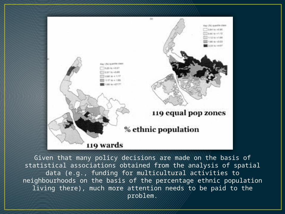
Given that many policy decisions are made on the basis of statistical associations obtained from the analysis of spatial data (e.g., funding for multicultural activities to

neighbourhoods on the basis of the percentage ethnic population living there), much more attention needs to be paid to the problem.

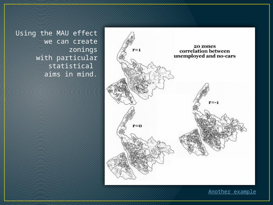
Using the MAU effect we can create zonings

with particular statistical aims in mind.

Another example

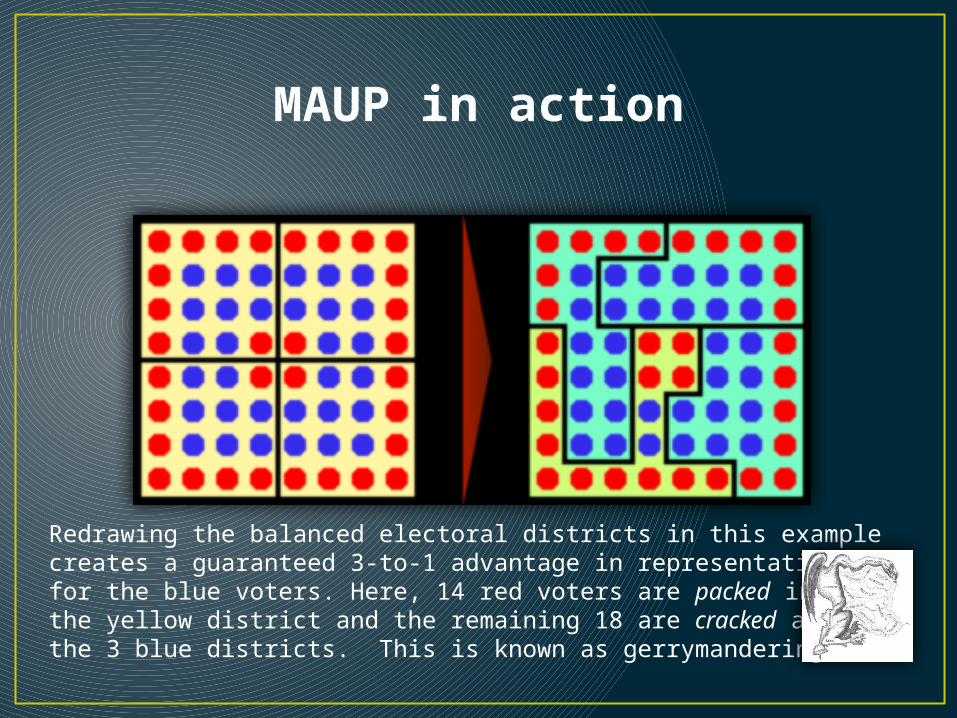
MAUP in action

Redrawing the balanced electoral districts in this example creates a guaranteed 3-to-1 advantage in representation for the blue voters. Here, 14 red voters are packed into the yellow district and the remaining 18 are cracked across the 3 blue districts. This is known as gerrymandering.

Gerrymandering

• The MAUP is a very real issue for politicians.• One of the requirements of Civil Rights era

legislation is that states that had a history of racial discrimination (generally, the states that constituted the Confederacy, including Texas) must obtain "pre-clearance" of all redistricting plans from the U.S. Department of Justice. This is because of the tendency of those states to engage in so-called "racial gerrymandering" – configuring districts in order to minimize minority representation. This can be done either by concentrating minorities in as few districts as possible (minority vote concentration), or distributing them across many districts (minority vote dilution).

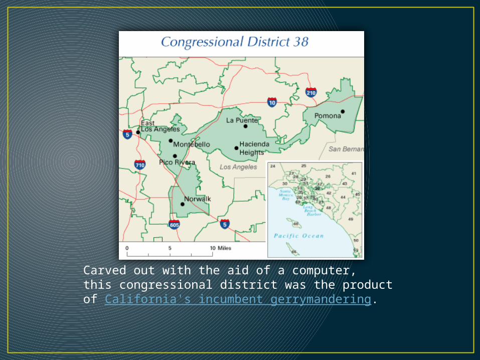
Carved out with the aid of a computer, this congressional district was the product of California's incumbent gerrymandering.

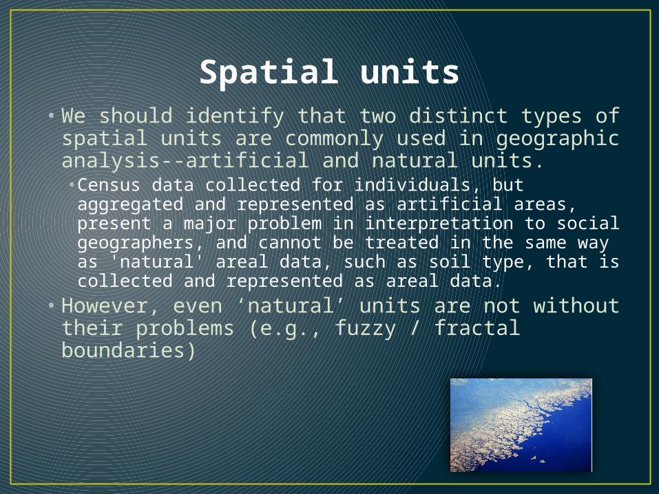
Spatial units• We should identify that two distinct types of

spatial units are commonly used in geographic analysis--artificial and natural units. • Census data collected for individuals, but aggregated and represented as artificial areas, present a major problem in interpretation to social geographers, and cannot be treated in the same way as 'natural' areal data, such as soil type, that is collected and represented as areal data.

• However, even ‘natural’ units are not without their problems (e.g., fuzzy / fractal boundaries)

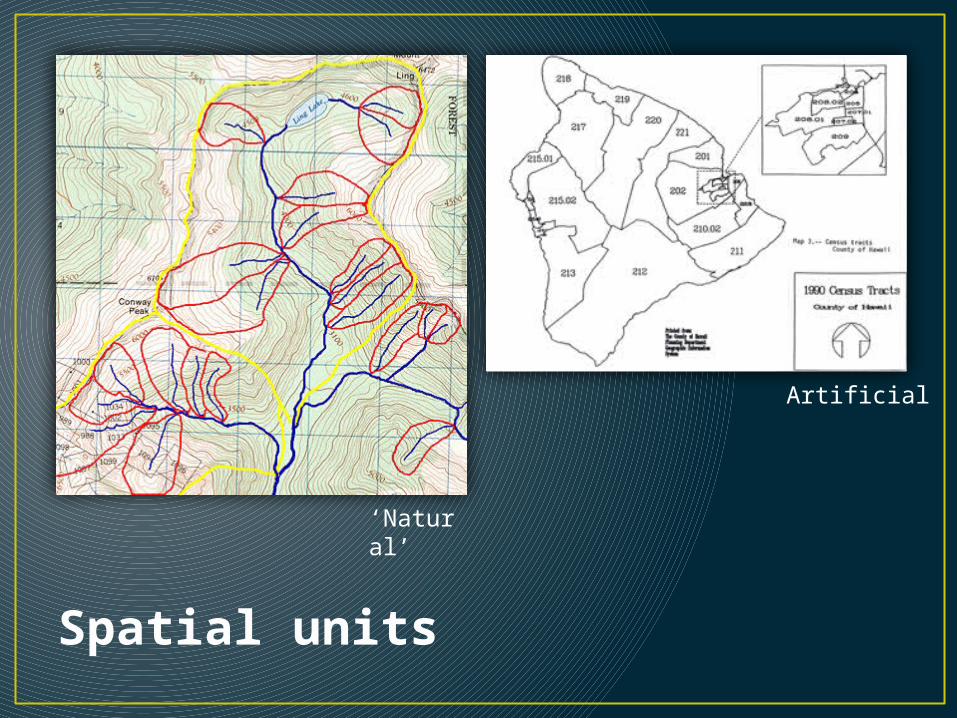
Spatial units

Artificial

‘Natural’

Simpson’s paradox

• However, there are other elements which may impact any study using aggregated data.• Simpson's Paradox is commonly encountered.

• If the values of the variables vary in correlation with another (e.g., areas with high unemployment rates are often associated with areas that also exhibit high rates of other social-economic characteristics), then it may be impossible to obtain a reliable estimate of the true correlation between two variables.

Example

Simpson’s paradox

• The paradox in the example arises because we assume that race is the independent variable while unemployment is the dependent variable. In fact, location is the independent variable (and unavailable for examination when we only examine the totals) and unemployment and race are the dependent variables.

• An example of a common-response relation.

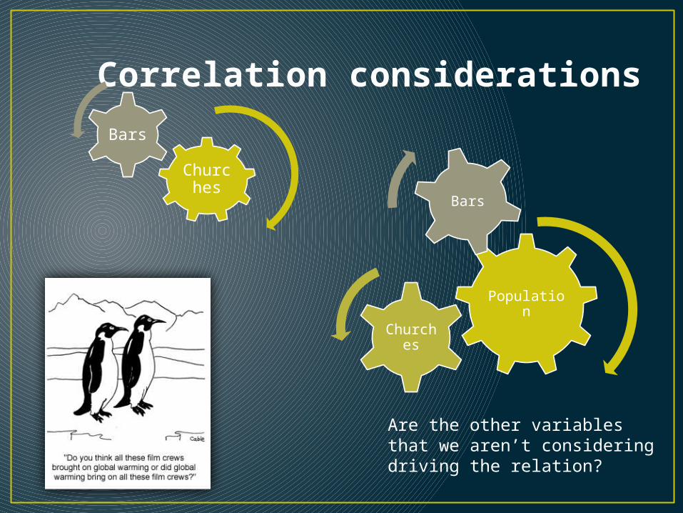
Correlation considerations

Churches

Bars

Population

Churches

Bars

Are the other variables that we aren’t consideringdriving the relation?

Why does the MAUP exist?

• Geographical areas are made up not of random groupings of individuals / households, but of individuals / households that tend to be more alike within the area than to those outside of the area. Three main classes of models have been identified: • Grouping• Group-dependent• Feedback

Neighbourhood models

• Grouping models, in which similar individuals / households choose, or are constrained, to locate in the same area / group, either when those groups are formed or through migrations.

• That is to say, some process has operated and / or continues to operate such that individuals / households do not randomly move into areas. (Chinatown, Sikh neighbourhoods in Surrey)

• A tendency for plants with similar ecological requirements to be located in 'communities'.

Neighbourhood models• Group-dependent models, in which individuals

/ households in the same area / group are subject to similar external influences.

• For example, there may be some 'contextual' variable affecting all individuals in the area. Alternatively, some common influence may have operated in the past, the effects of which are still felt (e.g., the restrictive covenants that used to be in place in the British properties in West Vancouver).

• The rain shadow effects felt in the Okanagan Valley, and the dryland communities that result.

Neighbourhood models• Feedback models, in which individuals /

households interact with each other and influence each other, and the frequency / strength of such interaction is likely to be greater between individuals in the same area / group than between individuals in different areas. (A tendency for people living nearby to interact and as a result to develop common characteristics.)

• A bog community, wherein the acid conditions are maintained by the decomposition of the plants found therein.

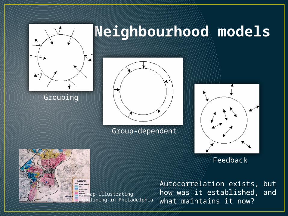
Neighbourhood models

Grouping

Group-dependent

Feedback

A map illustratingredlining in Philadelphia

Autocorrelation exists, but how was it established, andwhat maintains it now?

Neighbourhood models

• These models could all be operating, and be operating at different scales (block, neighbourhood, city, province).

• Therefore, attempting to achieve a perfect understanding of the reasons why MAUP occurs may be impossible. These models describe different ways in which spatial (auto)correlation may be acting on the variables of interest.

Conclusion

• So, as you can see, developing an understanding of the role that geography alone can play in an analysis is vital--before one can search for meaningful biological, environmental or sociological explanations for an observation, one should first eliminate the geographic explanation.

• Ultimately, neighbourhoods are composed of unique combinations of biological (behavioral, social, political, economic) and physical environments (all of which might change over time), and no combination of statistical manipulations may be able to unpack such a complex set of 'actors.'