Embed Size (px)
Citation preview

THE PRICING OF HEDGING LONGEVITY RISK WITH THE HELP
OF ANNUITY SECURITIZATIONS: AN APPLICATION TO THE
GERMAN MARKET
JONAS LORSON
JOËL WAGNER
WORKING PAPERS ON RISK MANAGEMENT AND INSURANCE NO. 118
EDITED BY HATO SCHMEISER
CHAIR FOR RISK MANAGEMENT AND INSURANCE
OCTOBER 2012
Working Papers on Risk Management and Insurance No. 118 - October 2012
The Pricing of Hedging Longevity Risk
with the Help of Annuity Securitizations:
An Application to the German Market
Jonas Lorson, Joel Wagner!
Abstract
Prolongation of life expectancy implies a severe risk for annuity providers. Insurance companies
can use securitization transactions to address this longevity risk in their portfolios. Securitization can
serve as a substitute for classic reinsurance since it also transfers risk to third parties. We develop
a model to hedge annuity portfolios against increases in life expectancy. By doing so, we forecast
future mortality rates with the Lee-Carter-model and use the Wang-transformation to incorporate
insurance risk. Based on the percentile tranching method, where individual tranches are aligned to
Standard & Poor’s ratings, we price an inverse survivor bond. This bond o!ers fix coupon payments
to investors while the principal payments are at risk and depend on the survival rate within the
underlying portfolio. Finally, we apply this securitization structure to calculate the securitization
prices for a sample portfolio from a large life insurance company.
Key words Life Securitization · Longevity Risk · Insurance Pricing and Hedging · Inverse Survivor
Bond · Percentile Tranching
JEL Classification G12 · G17 · G22 · G23
1 Introduction
Across the globe, and in the industrial nations in particular, people have seen an unprecedented increase
in their life expectancy over the last decades (see, for example, MacDonald et al., 1998). The benefits
of this apply to the individual, but the dangers apply to annuity providers. Insurance companies often
possess no e!ective tools to address the longevity risk inherent in their annuity portfolio. However, they
can use the financial markets to mitigate the negative implications from an increase in life expectancy
to their risk position by securitizing parts of their portfolio. The synthetic securitization acts as a hedge
for the insurer’s portfolio: the securitization deal transfers the risks of the portfolio to third parties and
serves as a substitute for reinsurance.!Jonas Lorson and Joel Wagner are with the Institute of Insurance Economics, University of St. Gallen, Kirchlistrasse 2,
CH-9010 St. Gallen.
1
Working Papers on Risk Management and Insurance No. 118 - October 2012
In contrast to non-life segments, where securitization transactions such as CAT bonds are an estab-
lished instrument now and account for high volumes, the life securitization market is still in its infancy
(see, e.g., Deutsche Bank, 2010). The first mortality-linked securitization transaction was carried out by
Swiss Re in 2003. The issue of the Vita Capital bond for a three-year time period reduced Swiss Re’s
exposure resulting from shifts in mortality. This bond had principal payments which were dependent on
the development of a predefined mortality index (Blake et al., 2006). Another attempt at a longevity bond
occurred in 2004. The European Investment Bank tried to issue, with the help of BNP Paribas, a bond
with coupon payment depending on the survival of English and Welsh males aged 65 in the year 2002.
The duration of the contract was intended to be 25 years and the total volume to be £ 540 mn. However,
the transaction did not attract enough investors and was abandoned in 2005 (Chen and Cummins, 2010).
After these initial attempts, the life securitization market gained momentum with increasing volumes
and transactions until 2007. However, with the beginning of the financial crisis, the issuing of life secu-
ritizations dropped significantly and is still in a recovery phase today (for a detailed review, see Section 2).
The literature o!ers a variety of models for hedging longevity risk. Among them, Wang et al. (2011)
apply the concept of reverse mortgages to hedge longevity risk for life insurance companies. Wang et al.
(2010) use a model to determine the optimal annuity product mix to receive a natural hedge against
longevity risk, while Luciano et al. (2012) make use of Delta-Gamma hedging. In the paper by Gatzert
and Wesker (2012), the authors consider a “natural” hedge between life insurance and annuities in order to
reduce net portfolio exposure to systemic mortality risk. Another approach is the annuity securitization:
Kim and Choi (2011) present a method for securitizing longevity risk with the help of percentile tranching
using a coupon-at-risk calculation (see also, for instance, Wills and Sherris, 2010, or Bae et al., 2009).
The authors apply the concept of an inverse survivor bond to a fictional portfolio of Australian annuity
contracts. Their focus lies on the yield that investors can achieve with an investment in such a bond. Our
approach is closest to that of Kim and Choi (2011). We make use of a percentile tranching method directly
linking chosen percentiles to Standard & Poor’s (S&P) rating classes for insurance-linked securities. By
doing so, investors receive a clear picture of the quality of the securitization tranche they are investing
in. In addition, the issuer has the possibility to approach specific investor types in terms of risk-attitude
directly with its securitization o!er. Typically, the coupon payments are put at risk within an inverse
survivor bond. The insurer receives on the issuing date cash flow from investors which can be considered
a loan. This loan is then repaid to the creditors with an annual principal amount over the entire maturity
of the bond. The principal payments are of equal size for each period; however, their full repayment
remains subject to the actual survival rates within the underlying portfolio. In addition, the investors
receive at each time period the respective coupon rate, which is tranche specific. Within this securitization
structure, the insurer receives the loan from the investors and can use this money to generate capital
returns. At the end of the transaction, the full loan has been paid back to the investors and the coupon
payments depend on the portfolio’s survival rates. In the current low interest capital market environment,
it is doubtful if this structure is still advantageous for the insurer since the ability to generate su"cient
capital returns with the borrowed money to cover potential additional payments from longevity increases
might be limited. Thus, and in order to ensure that enough capital is available, our model is based on
2
Working Papers on Risk Management and Insurance No. 118 - October 2012
the payment of fixed coupon rates and variable repayments of the principal (principal-at-risk approach).
In this paper, we extend on methods insurer’s can use to hedge their annuity portfolio against longevity
risk with the help of annuity securitization. To do so, we take the perspective of the issuing insurance
company and calculate the costs of hedging in a four step process. First, we calculate future mortality
rates using the classic Lee-Carter-model (Lee and Carter, 1992). In a second step, we adapt the fore-
casted mortality rates with the help of the transformation by Wang (2000) in order to incorporate the
price of risk in the insurance contract. We then apply the transformed death rates to the annuitants
of our sample portfolio. Third, we slice the forecasted annuity portfolio into di!erent tranches with the
help of the percentile tranching method (analogous to Kim and Choi, 2011). Thereby, we use attachment
and detachment points for the individual tranches corresponding to S&P ratings for insurance-linked
securities. In a last step, we price the di!erent tranches of our annuity securitization with the help of
classical bond pricing. The principal payments that investors receive are a random variable and depend
on the survival distribution of the underlying portfolio. If the number of actual survivors is higher than
expected, the amount of principal payment is reduced according to the determined tranche levels. To
illustrate the implication of this bond structure, we finally conduct several sensitivity tests before we
apply our pricing model to the retail sample annuity portfolio from a leading German life insurer. The
contribution to the academic literature is threefold. On the theoretical side, building on the work of Kim
and Choi (2011), we adapt their pricing model to the current market situation. Putting the principal
at risk instead of the coupon payments, the insurer is supplied with su"cient capital in order to cover
additional costs due to longevity. On the empirical side, we specify the method for the German market.
Inserting specific country data into the model, we analyze price sensitivities of the presented securitiza-
tion model. Finally, in a case study, we apply the procedure to the annuity portfolio of a large German
life insurer and calculate the price of hedging longevity risk.
The remainder of this paper is organized as follows. In Section 2, the theoretical background of
securitization in general, and life insurance securitization in particular, is discussed as well as the related
literature review. The concept of inverse survivor bonds is explained in detail. Section 3 presents the
mathematical calculus of an annuity securitization, from the definition of future mortality rates with
the help of the Lee-Carter-model up to the pricing of single securitization tranches. Section 4 presents
numerical outcomes and shows the dynamics and sensitivities of our model. Afterwards, Section 5 applies
the model to a real-world annuity portfolio from a large life insurance company. Section 6 summarizes
the presented results and concludes.
2 Literature review and securitization market overview
With the recent financial crisis in mind – and its being caused by unsound structuring of mortgage
loans – securitization is still of major interest for financial service providers in general and insurance
companies in particular. In contrast to the banking sector where securitization, via asset-backed securities
or collateralized debt obligations for instance, hit huge levels before the financial crisis, life insurance
companies are still very cautious about these transactions despite potential benefits (see, for example,
3
Working Papers on Risk Management and Insurance No. 118 - October 2012
De Mey, 2007, or Beltratti and Corvino, 2008, for a review). In general, securitization can be defined
as the “repackaging and trading of cash flows that traditionally would have been held on-balance-sheet”
(Cummins and Weiss, 2009, p. 515). The purpose of this trading lies in the diversification of risk.
There are manifold explanations why securitization transactions are beneficial for life insurers. Ac-
cording to Cowley and Cummins (2005), a reduction of costs of capital as well as an increase in the return
on equity are the main advantages. Through securitization, unlocking embedded profits in the balance
sheet becomes possible for the issuer. In addition, this financial instrument can serve as an alternative
possibility to financing. Furthermore, the transparency of many on-balance-sheet assets and liabilities –
traditionally characterized by a certain degree of illiquidity, complexity, and informational opacity – is
improved by securitization (Cowley and Cummins, 2005, p. 194). Other players in the financial market
can also benefit from these transactions. Life securitization introduces a new asset class with almost no
correlation to other investments (see also Lin and Cox, 2008). The true driver of life portfolios lies in the
life expectancy of the policyholders – and this is not a!ected by the development of yield curves or stock
market returns. Consequently, institutional investors should be able to reduce their overall portfolio risk
by adding life securitization to their investments (see, for example, Litzenberger et al., 1996, and Deng
et al., 2012). From a regulatory perspective, it is expected that securitization will be treated under Sol-
vency II analogous to reinsurance when it comes to the determination of standard capital requirements
(Cummins and Trainar, 2009, p. 489). At the same time, it enables third parties to invest in insurance
products without possessing an insurance license by acting as investors to the securitization.
Historic life securitization transactions
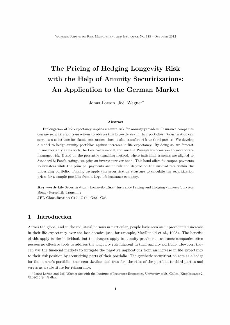
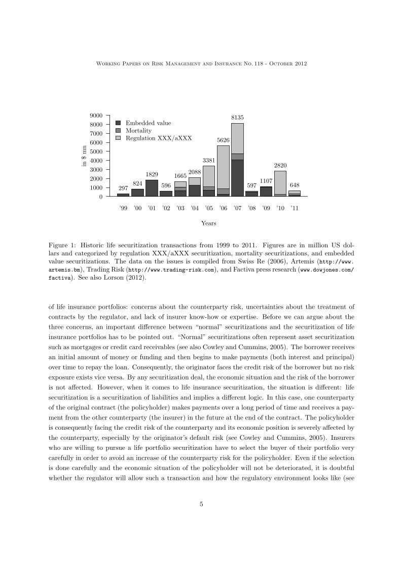
Figure 1 shows an aggregation of the issued life securitizations from 1999 to 2011. The deals are clustered
into three di!erent categories: regulation XXX/aXXX securitization deals,1 mortality securitizations
and embedded value securitizations. Historically, the maximum total amount of life securitization was
achieved in 2007 with a volume of $ 8.1 bn. The amount of transaction volumes then drops significantly
with the start of the financial crisis in 2008 to $ 0.6 bn. In comparison with the assets on the balance
sheets of life insurers, the volume of these transactions is totally negligible even in years with extensive
usage of this instrument. On average, the securitized deal had a size of $ 417 mn while the median of the
transaction volumes is $ 300 mn. The top three issuing companies in terms of total volume are Aegon
($ 3.7 bn), Scottish Re ($ 3.6 bn), and Genworth ($ 3.5 bn). In total, insurance companies undertook
71 life securitization transactions from 1999 to 2011, of which 31 were embedded value, 31 regulation
XXX/aXXX transactions and 9 mortality transactions. In that period, primary insurers securitized life
products in 48 deals with a value of $ 21.6 bn and reinsurance companies transferred a volume of $ 8.4 bn
with the help of 23 transactions. Further information on observed life securitization deals can be found
in, e.g., Lorson (2012).
An explanation for the relatively low transaction volumes in comparison to the balance sheet assets of
life insurers can be found in D’Arcy and France (1992). The concerns for the usage of insurance futures
based on catastrophy loss indices stated by the author in 1992 still hold true today for the securitization
1Issuing of debt securities on insurer’s capital reserve requirements for term life products. More details on the di!erentcategories can be found in, e.g., Kampa (2010) or Cowley and Cummins (2005).
4
Working Papers on Risk Management and Insurance No. 118 - October 2012
’99 ’00 ’01 ’02 ’03 ’04 ’05 ’06 ’07 ’08 ’09 ’10 ’11
Years
in $
mn
0
1000
2000
3000
4000
5000
6000
7000
8000
9000Embedded valueMortalityRegulation XXX/aXXX
297824
1829
596
16652088
3381
5626
8135
5971107
2820
648
Figure 1: Historic life securitization transactions from 1999 to 2011. Figures are in million US dol-lars and categorized by regulation XXX/aXXX securitization, mortality securitizations, and embeddedvalue securitizations. The data on the issues is compiled from Swiss Re (2006), Artemis (http://www.artemis.bm), Trading Risk (http://www.trading-risk.com), and Factiva press research (www.dowjones.com/factiva). See also Lorson (2012).
of life insurance portfolios: concerns about the counterparty risk, uncertainties about the treatment of
contracts by the regulator, and lack of insurer know-how or expertise. Before we can argue about the
three concerns, an important di!erence between “normal” securitizations and the securitization of life
insurance portfolios has to be pointed out. “Normal” securitizations often represent asset securitization
such as mortgages or credit card receivables (see also Cowley and Cummins, 2005). The borrower receives
an initial amount of money or funding and then begins to make payments (both interest and principal)
over time to repay the loan. Consequently, the originator faces the credit risk of the borrower but no risk
exposure exists vice versa. By any securitization deal, the economic situation and the risk of the borrower
is not a!ected. However, when it comes to life insurance securitization, the situation is di!erent: life
securitization is a securitization of liabilities and implies a di!erent logic. In this case, one counterparty
of the original contract (the policyholder) makes payments over a long period of time and receives a pay-
ment from the other counterparty (the insurer) in the future at the end of the contract. The policyholder
is consequently facing the credit risk of the counterparty and its economic position is severely a!ected by
the counterparty, especially by the originator’s default risk (see Cowley and Cummins, 2005). Insurers
who are willing to pursue a life portfolio securitization have to select the buyer of their portfolio very
carefully in order to avoid an increase of the counterparty risk for the policyholder. Even if the selection
is done carefully and the economic situation of the policyholder will not be deteriorated, it is doubtful
whether the regulator will allow such a transaction and how the regulatory environment looks like (see
5
Working Papers on Risk Management and Insurance No. 118 - October 2012
for example Cummins and Weiss, 2009).
Classification of securitization deals
When it comes to classifying securitization deals, Cummins and Weiss (2009) divide the securitization
primarily into two di!erent categories: the asset-backed securities such as securities backed by corporate
bonds or mortgages, and the non-asset-backed products with examples like futures and options. The first
are usually backed by the underlying asset that is securitized, the latter are normally guaranteed by the
counterparty of the transaction and/or by an exchange. Both types of securitizations have in common
that they can be traded in an organized exchange environment as well as over-the-counter. Through
securitization, investors that do not possess an insurance license have access to insurance cash flows (Cox
and Schwebach, 1992). This further facilitates the diversification of risk in the entire financial market.
An insurer deciding to undergo a life insurance securitization has, at least theoretically, two possibili-
ties to proceed. The first one is a true sale of the assets which should be securitized, and the second one is
a synthetic securitization. In the case of a “true” securitization the insurer would securitize its portfolio
(or parts of it) by selling the contracts to investors in di!erent tranches. In contrast to the banking sector
where true sale transactions occur daily, this type of securitization does not take place in the insurance
industry. The main reason for this is legal issues. As mentioned before, in life insurance the economic
position of the policyholder is severely a!ected by the counterparty since the fulfillment of the service
promise lies in the future. It is very doubtful if a regulatory authority would allow such transactions in
which the counterparty obligation fades from a supervised insurance company to third party investors.
In addition, such a deal would result in a giant time horizon of commitment for the investors. Contract
durations of more than 60 years are not uncommon (for instance in the case of classic pension products).
Only few investors might be interested in engaging in such long transactions. Furthermore, a potential
investor would face several operational problems in a true sale life securitization: he must provide the
necessary systems for the premium collection, for instance, or take care of the asset management. Con-
sequently, to the best of our knowledge, there has been no true sale life securitization so far. The second
option, “synthetic” securitization (or “synthetic” sale) is the common method for annuity securitization.
Within this approach, accounting for the contracts and carrying of risks remains with the insurance com-
pany. In most cases, a special purpose vehicle is established to serve as an intermediary for cash flows
between the issuer and the investors. The transaction is simply a securitization of cash flows.
Models for life securitization and pricing
Several models for life securitization approaches can be found in the literature. Blake and Burrows (2001)
proposes the issuing of survivor bonds whereby the coupon payment which investors receive depend on
the mortality rates of a specified population and are thus a random variable (see also Dowd, 2003, and
Blake, 2003). This construct of survivor bonds is also applied by Denuit et al. (2007). Other possibilities
to hedge longevity risk are survivor options or swaps and futures, which are discussed, for example, by
Cox and Lin (2007). Survivor swaps comprise the exchange of cash flows between two parties with a
6
Working Papers on Risk Management and Insurance No. 118 - October 2012
fixed cash flow in the present and an uncertain future cash flow depending on the mortality of a specified
group (see, for example, Dowd et al., 2006). Cox et al. (2006) consider the first mortality securitization
by Swiss Re in 2003 and use multivariate exponential tilting to price this transaction. Lin and Cox
(2005) develop a model for analyzing mortality-based securities, in particular mortality bonds and swaps,
and price these contracts (by applying the one factor Wang transformation). Cox et al. (2010) integrate
permanent longevity jump processes as well as a temporary jump process in mortality to the Lee-Carter-
model and use the derived forecasted mortality rates to price a longevity option with indi!erence pricing.
Lin and Cox (2008) use a two-factor Wang transformation to develop an asset pricing model for securities
based on mortality. Bauer et al. (2010) review existing pricing methods for longevity-linked securities and
present a longevity derivative that provides an option-type payo!. Also Dowd et al. (2006) use the idea of
survivor swaps to exchange future cash flows between the insurer and third parties based on a reference
survivor index. Wills and Sherris (2010) securitize a longevity bond with the help of Australian mortality
data. They calculate di!erent tranches by percentage cumulative loss and price these tranches. Bi"s and
Blake (2010) address in their study the e!ects of asymmetric information on longevity securitizations and
how they should be tranched under partial information. For further references on longevity securitization
research, we refer to the review by Blake et al. (2011).
Inverse survivor bonds
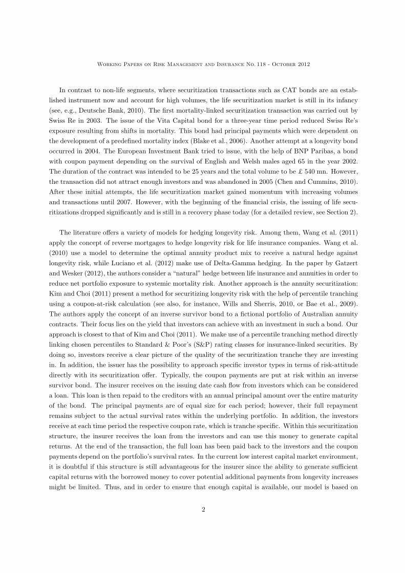
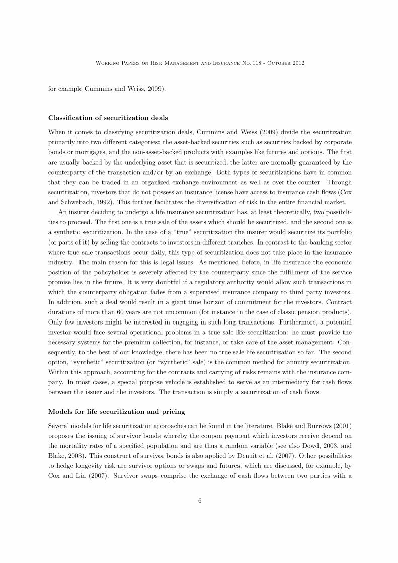
An inverse survivor bond is a special case of survivor bonds that insurance companies can use to hedge
their annuity portfolio against mortality changes. The structure of these bonds is illustrated in Figure 2.
Annuitants
Premiums
paid
Annuity
Issuer
Premium
Contingent
payment
Special purpose
vehicle (SPV)
Investment
into bond
Coupon &
principal
Investors
Tranche 1
Tranche 2
Tranche 3
. . .
Tranche N
Figure 2: Structure of an Inverse Survivor Bond (adapted from Wills and Sherris, 2010, and Kim andChoi, 2011).
At the center of the bond structure stands a special purpose vehicle (SPV). This legal entity brings
together the issuer (the insurance company) and the investors who want to engage in the annuity portfolio.
The insurer – while paying out the annuities to its annuitants – transfers the premiums received from the
annuity sales to the SPV. Following the investors participation in the bond, the SPV provides contingent
7

Working Papers on Risk Management and Insurance No. 118 - October 2012
payments to the insurance company (securing thus the annuity payments). On the investor side, the SPV
issues a survivor bond which pays regular coupon payments. Often, the principal is paid as a lump sum
at the maturity of the bond, while the coupon payment is paid annually and is subject to the survival
rate of the underlying portfolio, and thus at risk. The investor faces the risk that partial future coupon
rates or even all future coupon rates are lost if less annuitants than ex ante expected die within the
portfolio. In our consideration, as mentioned before, the principal payment will be at risk whereas the
coupon payments are secured.
In order to attract more investors and to o!er a tailored risk profile, the survivor bond is sliced
into di!erent tranches. Lane and Beckwith (2007) argue that tranching becomes more popular when
related to insurance-linked securities. Such bonds usually possess less than ten tranches, which can di!er
significantly in their risk profile. The investors in the first tranche are provided with the least coverage.
They are the first to lose their coupon or principal payments if the number of actual survivors in the
portfolio is higher than expected. If the first tranche is exceeded, the loss moves to the second tranche,
and so on. Due to the di!erent risk characteristics, each tranche has a di!erent price within the survivor
bond. In order to signal to investors the quality of the securitized portfolio, the first loss position (the
first tranche) is often kept by the issuer (see, for example, Gale and Hellwig, 1985, or Riddiough, 1997).
When maintaining the first loss position, the issuer has an incentive to closely monitor the correct and
timely premium collection and to price the portfolio conscientiously.
3 Calculation of the securitization of an annuity portfolio
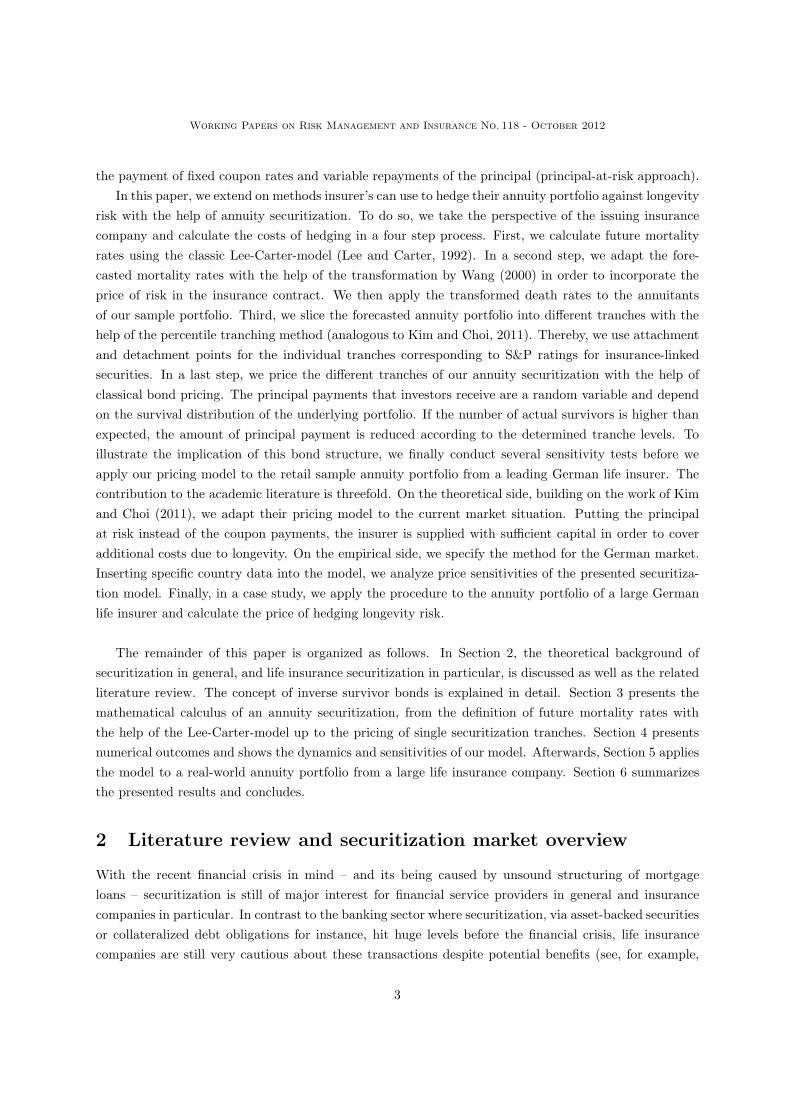
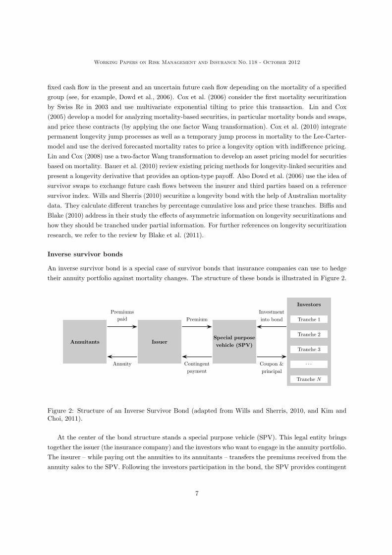
This section describes the calculus used to synthetically securitize a life annuity portfolio. We adapt the
model from Kim and Choi (2011) for an inverse survivor bond with the core di!erence that we set the
principal payment at risk and not coupon payment. Figure 3 illustrates our approach.
Based on historic life tables, Section 3.1 describes the application of the Lee-Carter-model in order to
forecast future mortality rates. Afterwards in Section 3.2, we adjust the derived survival probabilities for
the uncertainty in the mortality tables as well as the uncertainty of the annuitant’s lifetime. Therefore,
we use the Wang-transformation (Wang, 2000) to derive the adjusted survival probability distribution for
all ages x of annuitants and future years t = 1, . . . , T , where T denotes the duration of the securitization
contract. In Section 3.3 the di!erent attachment and detachment points for each observed tranche are
introduced. We define N tranches with the help of percentiles based on cumulative survival probabilities.
Based on these tranche limits, we derive the value of each individual tranche j, j = 1, . . . , N , for each
time t (until T ) and the face value FV of the entire inverse survivor bond. Using this face value we price
the individual tranches in Section 3.4 by calculating prices for the coupon payments as well as for the
principal payments for all contract years t. We assume that coupons and principals are paid once a year
at the end of the period. Finally, we derive the total price of securitization for a given annuitant aged x
by summing all tranches and contract years.
8
Working Papers on Risk Management and Insurance No. 118 - October 2012
Actual historic death rates
Forecasting future mortality rates with
the Lee-Carter model (Section 3.1)
Survival probablity distribution forecast for all ages and years
Adjustment for the market price of risk
using the Wang-transform (Section 3.2)
Adjusted survival probability distribution for all ages and years
Definition of attachment and detachmentpoints for the tranches (Section 3.3)
Sum of excess losses for each tranche (and age/year) define the bond face value
Calculation of tranche prices as sum
of coupon and principal (Section 3.4)
Total price of securitization (per age) given by sum of tranches and years
Figure 3: Approach for calculating the price of an annuity securitization.
3.1 Forecasting future mortality rates with the Lee-Carter model
A range of stochastic models for forecasting mortality rates have been developed in the last decade. The
earliest model was developed by Lee and Carter (Lee and Carter, 1992) and several researchers built on
and extended their work.2 The Lee-Carter-model is is still the most popular model and widely used in
the literature for valuating life portfolios and as a basis for insurance securitization (see, for example,
Denuit et al., 2007, or Kim and Choi, 2011).
The Lee-Carter-model is a discrete time series model that uses historic mortality rates to project the
future trend of mortality. It is based on the assumption that future mortality will continue to change at
the same rates as it did in the past. In the model, the fitted death rates m(x, t) for ages x at times t (see
2The most prominent models are those of Renshaw and Haberman (2006), De Jong and Tickle (2006), Delwarde et al.(2007), Czado et al. (2005), or Cairns et al. (2006).
9
Working Papers on Risk Management and Insurance No. 118 - October 2012
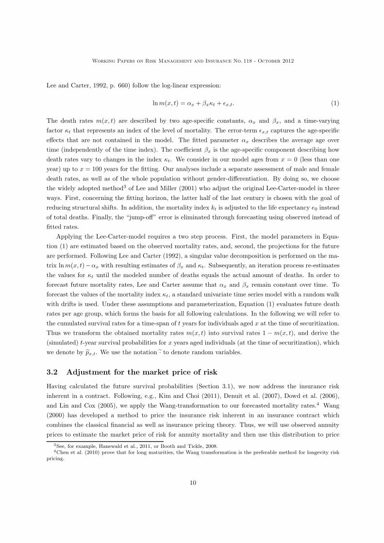
Lee and Carter, 1992, p. 660) follow the log-linear expression:
lnm(x, t) = !x + "x#t + $x,t. (1)
The death rates m(x, t) are described by two age-specific constants, !x and "x, and a time-varying
factor #t that represents an index of the level of mortality. The error-term $x,t captures the age-specific
e!ects that are not contained in the model. The fitted parameter !x describes the average age over
time (independently of the time index). The coe"cient "x is the age-specific component describing how
death rates vary to changes in the index #t. We consider in our model ages from x = 0 (less than one
year) up to x = 100 years for the fitting. Our analyses include a separate assessment of male and female
death rates, as well as of the whole population without gender-di!erentiation. By doing so, we choose
the widely adopted method3 of Lee and Miller (2001) who adjust the original Lee-Carter-model in three
ways. First, concerning the fitting horizon, the latter half of the last century is chosen with the goal of
reducing structural shifts. In addition, the mortality index kt is adjusted to the life expectancy e0 instead
of total deaths. Finally, the “jump-o!” error is eliminated through forecasting using observed instead of
fitted rates.
Applying the Lee-Carter-model requires a two step process. First, the model parameters in Equa-
tion (1) are estimated based on the observed mortality rates, and, second, the projections for the future
are performed. Following Lee and Carter (1992), a singular value decomposition is performed on the ma-
trix lnm(x, t)!!x with resulting estimates of "x and #t. Subsequently, an iteration process re-estimates
the values for #t until the modeled number of deaths equals the actual amount of deaths. In order to
forecast future mortality rates, Lee and Carter assume that !x and "x remain constant over time. To
forecast the values of the mortality index #t, a standard univariate time series model with a random walk
with drifts is used. Under these assumptions and parameterization, Equation (1) evaluates future death
rates per age group, which forms the basis for all following calculations. In the following we will refer to
the cumulated survival rates for a time-span of t years for individuals aged x at the time of securitization.
Thus we transform the obtained mortality rates m(x, t) into survival rates 1 ! m(x, t), and derive the
(simulated) t-year survival probabilities for x years aged individuals (at the time of securitization), which
we denote by !px,t. We use the notation !· to denote random variables.
3.2 Adjustment for the market price of risk
Having calculated the future survival probabilities (Section 3.1), we now address the insurance risk
inherent in a contract. Following, e.g., Kim and Choi (2011), Denuit et al. (2007), Dowd et al. (2006),
and Lin and Cox (2005), we apply the Wang-transformation to our forecasted mortality rates.4 Wang
(2000) has developed a method to price the insurance risk inherent in an insurance contract which
combines the classical financial as well as insurance pricing theory. Thus, we will use observed annuity
prices to estimate the market price of risk for annuity mortality and then use this distribution to price
3See, for example, Hanewald et al., 2011, or Booth and Tickle, 2008.4Chen et al. (2010) prove that for long maturities, the Wang transformation is the preferable method for longevity risk
pricing.
10
Working Papers on Risk Management and Insurance No. 118 - October 2012
bonds (see Lin and Cox, 2005). By doing so, the previously obtained survival rates !px,t are adapted for
the uncertainty in the mortality tables as well as the uncertainty in the lifetime of the annuitant.
If # denotes the standard normal cumulative distribution function and #!1 its inverse, Wang (2000,
p. 20) introduces the distortion operator described by
g! (u) = #"#!1 (u) + %
#, (2)
for all u with 0 < u < 1. The real-valued parameter % can be interpreted as the market price of risk.
Thus a function with given cumulative distribution function, F with values of !" < F < +" can be
transformed into a distorted distribution function F " with the help of the market price of risk % by the
following equation,
F " = 1 ! g!(1 ! F ) = #"#!1(1 ! F ) + %
#. (3)
In our framework, we apply the above formula and let F stand for the cumulative distribution function
of the future survival probabilities !px,t for ages x and years t. In the sequel we denote with !p!x,t the
so-transformed survival probabilities.
3.3 Tranche definition and excess loss per tranche
The next step involves the definition of individual tranches to be securitized and the calculation of the
excess loss for each tranche. We consider N di!erent tranches in our inverse survivor bond. The attach-
ment points p!(j!1)x,t and detachment points p!(j)x,t for tranche j, j = 1, . . . , N , are defined as a percentile
of the cumulative survival distribution based on the Wang-transformed values. Here our approach dif-
fers from Kim and Choi (2011, p. 15, Fig. 12). These authors define the attachment point of the first
tranche p!(0)x,t at the median survival probability or 50%-tile. In order to derive results from financial
markets practice, we link the attachment points to the tranches according to the S&P default table for
insurance-linked securities.5 S&P provides cumulative default probabilities for di!erent rating classes and
di!erent maturities. In Table 9 (see Appendix 7.2) we report the S&P cumulative default probabilities
for insurance-linked securitizations corresponding to the rating classes AAA to B– and maturities ranging
from T = 1 to 30 years. In our application, the detachment point of the last tranche is defined as the
100%-tile of the survival distribution, i.e. p!(N)x,t = 1 (100%-tile). The attachment and detachment points
for the remaining tranches can be flexible and defined according to the intended tranche composition
of the securitization. The percentile below the attachment point of the first tranche p!(0)x is the part
retained by the issuer. It can be considered as a first loss position. In our further applications, we will,
e.g., define the attachment p!(0)x,t equal to the percentile of the S&P B+ tranche, which corresponds to
an approximately 30% cumulative default probability within 10 years. For further tranches we consider
BBB–, A, and AAA in our reference case (see Table 4). The face value FV of the bond can also be
readily calculated. It corresponds to the di!erence between the 100%-tile of the survival distribution and
the attachment point of the first tranche (p!(0)x,t ).
5See S&P default tables from 2008, http://www.standardandpoors.com.
11

Working Papers on Risk Management and Insurance No. 118 - October 2012
To calculate the excess loss for each tranche, we assume that the insurer pays 1 (one) currency unit to
each annuitant who survives each year. In the following, we suppose the attachment points p!(j!1)x,t and
the detachment points p!(j)x,t for each tranche j, j = 1, . . . , N given. Let lx represent the initial population
of annuitants of age x at the beginning of the securitization (t = 0). Thus the actual number of survivors
in each group (tranche) is a random variable driven by the numerically simulated distribution of survival
rates !px,t, and l!x+t = lx · !p!x,t describes the actual number of survivors at age x + t. Furthermore, and
with the yearly annuity payment set to unity, it follows that l(j)x+t = lx · p!(j)x,t denotes the actual amount
of losses linked to the attachment/detachment points (see also Kim and Choi, 2011, pp. 11 and 16).
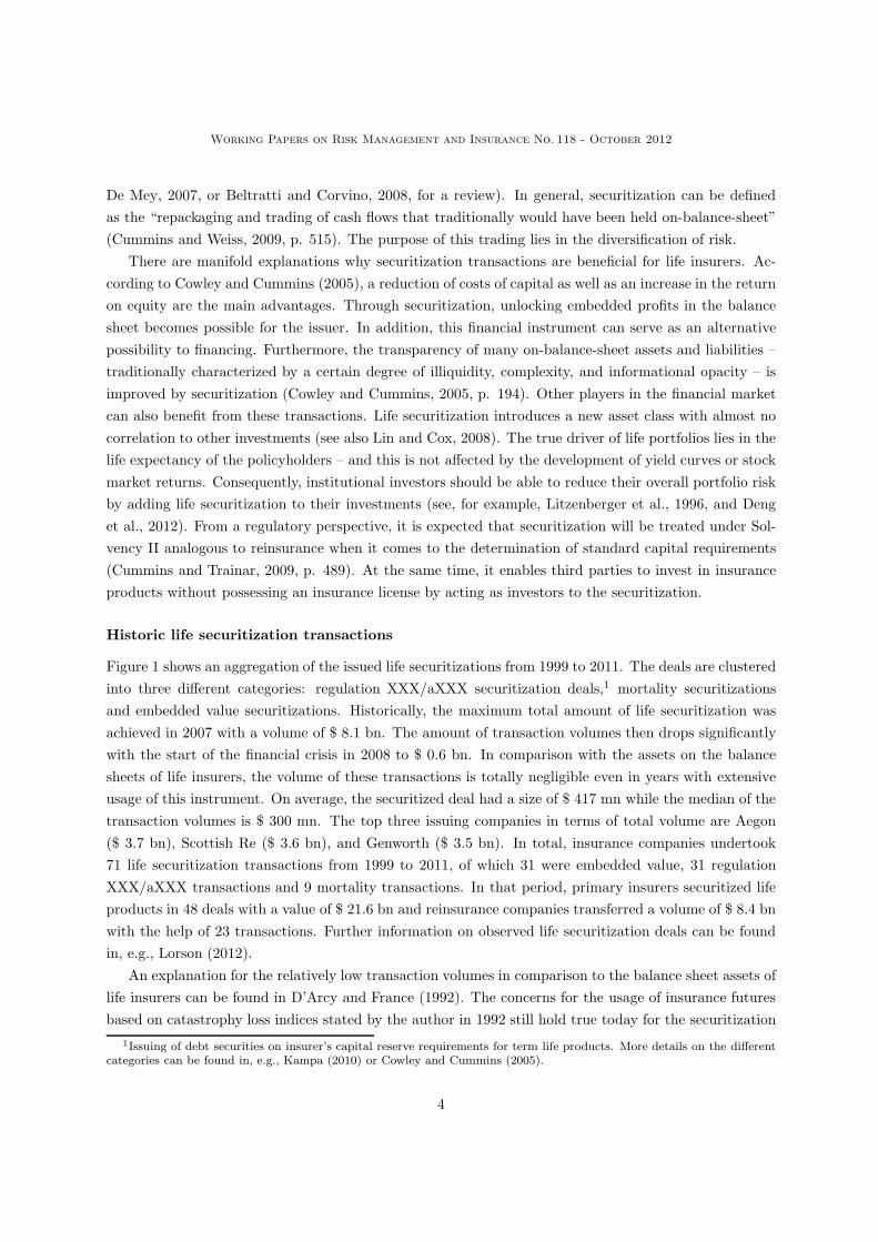
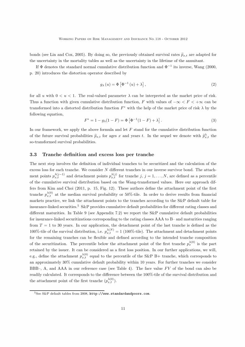
With the above notations, we are able to derive the calculation of the excess of loss. We illustrate our
proceeding in Figure 4. Each dot in Figure 4 represents one realization of the simulation run for the life
expectancy of an x years aged individual at a given time t after securitization. The dashed lines indicate
the attachment and detachment points of the observed tranche j (at time t). If a survival realization lies
within the borders of the loss that the considered tranche j has to bear – in line with the definition of the
respective attachment and detachment points – the tranche is triggered by the grey shaded loss. Thus
the excess loss for the jth tranche for individuals aged x at the time of securitization and t years after
securitization, denoted by L(j)x+t, is a random variable and can be described by
!L(j)x+t =
$l!x+t ! l(j!1)
x+t
%+!$l!x+t ! l(j)x+t
%+, (4)
where [·]+ stands for max(0, ·).
Having determined the excess loss for the tranche, the cash flows to the investors have to be calculated
accordingly. A reduction by the excess loss can be applied to the coupon rate or the principal payment of
the inverse survivor bond. While existing literature often discusses the case of a reduction of the coupon
rate, both models can be found in practice. In our model, if a tranche is triggered by an amount of
survivors that is higher than expected, the principal payment of this tranche is reduced proportionally.
Therefore, a proportion factor of default is introduced for each tranche j and time t that is defined by
!$(j)x+t =
!L(j)x+t
l(j)x+t ! l(j!1)x+t
, (5)
where we have 0 # !$(j)x+t # 1. This factor represents the loss percentage that is inherent in the jth
tranche, given the amount of survivors for the observed realization. It corresponds to the ratio of the
realized excess loss !L(j)x+t in the tranche and the “width” of the tranche given by l(j)x+t ! l(j!1)
x+t .
3.4 Pricing of the inverse survivor bond
The mechanism used for pricing the single tranches and the annuity securitization is as follows. As with
any other bond, the price of the inverse survivor bond consists of two parts, the coupon payment and the
principal payment.
The bond is structured in a way that the back payment of the nominal face value FV is distributed
over the duration of the contract T with T equally sized payments defined by FV/T . Since the principal
12
Working Papers on Risk Management and Insurance No. 118 - October 2012
Attachment point
l(j!1)x+t = lx · p!(j!1)
x,t
Detachment point
l(j)x+t = lx · p!(j)x,t
Actual number
of survivors l!x+t
Tranche j
Survival realization l!x+t
Borne loss !L(j)x+t by tranche j
for given survival realization l!x+t
Figure 4: Illustration of the excess loss !L(j)x+t calculation (see Equation 4) for tranche j at time t for
annuitants aged x + t (age x at the time of securitization).
payment is put at risk, it becomes a random variable which is expressed by
!P(j)x+t =
&1 ! !$(j)
x+t
'·FV
T, (6)
for the tranches j = 1, . . . , N and the annuitants’ ages x + t (t = 1, . . . , T ). The principal is inversely
proportionate to the amount of losses or, framed di!erently, to the amount of survivors in our portfolio.
The principal’s value can vary between 0, in the case where the actual survival rate is greater than the
detachment points of the jth tranche, and the full payment of FV/T , in the case where the actual survival
rate is lower than the corresponding attachment point of the jth tranche, i.e., we have 0 # !P(j)x+t #
FVT
.
The coupon payment is based on the outstanding principal and is paid annually. The applied annual
interest rate c(j) for each tranche j is comprised of a reference yield y such as, for instance, LIBOR
or EURIBOR, and a tranche-specific spread s(j), i.e., c(j) = y + s(j). The basis for the calculation
of the interest amount is defined by the outstanding amount of debt towards the investor given by
Dt = FV ! (t! 1) · FV/T = (T ! t + 1) · FV/T . Thus the coupon payment is given by
C(j)t = Dt · c
(j) = (T ! t + 1) ·FV
T·&y + s(j)
', (7)
for all tranches j = 1, . . . , N in times t = 1, . . . , T .
On the basis of the principal and coupon payments for each year and tranche along to the realized ex-
cess loss, the price of the inverse survivor bond can be derived with the help of the general bond equation.
13

Working Papers on Risk Management and Insurance No. 118 - October 2012
The bond price P (j)x in time t = 0 for an x years aged individual (at the time of securitization) and for
tranches j = 1, . . . , N , corresponds to the sum of the present value of (or expected value of discounted)
principal payments P (j),Px and the sum of all discounted coupon P (j),C
x payments until contract maturity
T . The price P (j)x is given by
P (j)x = P (j),P
x + P (j),Cx
=T(
t=1
E&!P(j)x+t · (1 + rf)
!t'
+T(
t=1
C(j)t · (1 + rf)
!t
=T(
t=1
1
(1 + rf)t·$E&!P(j)x+t
'+ C
(j)t
%
=FV
T·
T(
t=1
1
(1 + rf)t·$E&1 ! !$(j)
x+t
'+ (T ! t + 1) ·
&y + s(j)
'%, (8)
with rf the risk-free interest and E(·) denoting the expected value operator.
4 Numerical implementation and results
The aim of this section is to apply the previously introduced model step-by-step to the German market
and to link the definition of the tranches to S&P ratings. Thus we will be able to compare the prices for
di!erent portfolio structures (di!erent definition of the tranches) and perform selected sensitivity analysis
on the example of the results for a 65 year-old annuitant at the moment of securitization and unity (e 1)
annual pension claims.
4.1 Forecasting future mortality rates for Germany
In all industrial societies, the life expectancy of the population has risen continuously over the last
decades. This also holds true for Germany. As the basis for our calculations, we use German historic
mortality rates from the years 1960 to 2009. Thereby we combine the reported values of the Federal
Republic of Germany and the German Democratic Republic.6 For our study we proceed as described in
Section 3.1. For the analysis of the data on deaths and exposures as well as for the Lee-Carter forecasting
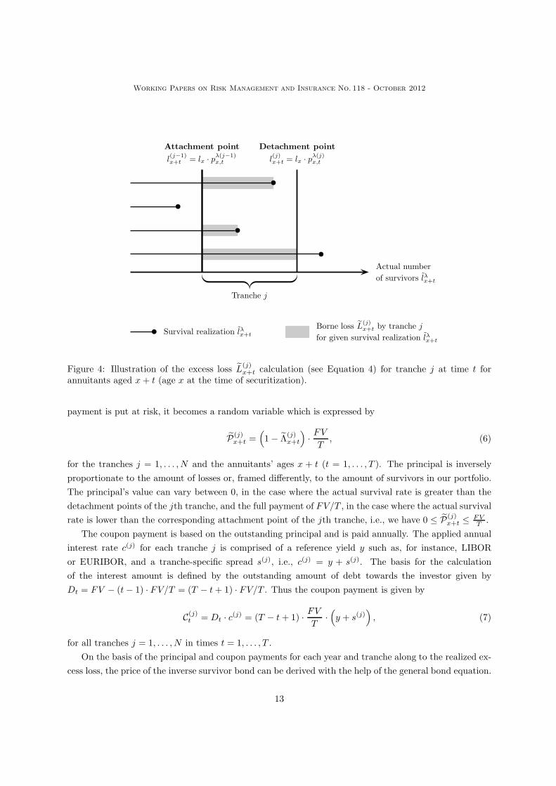
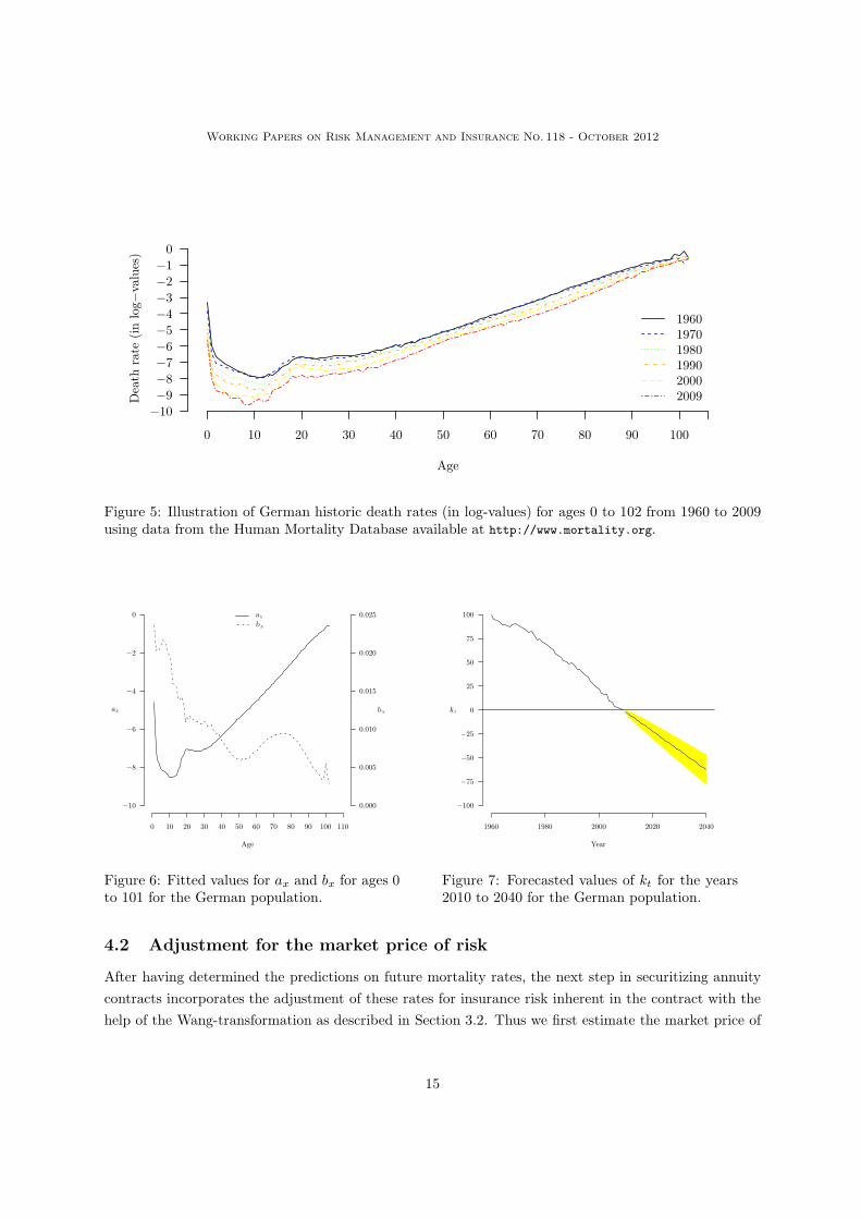
of mortality rates we use the R package ‘demography’.7 Figure 5 shows the historic age-specific death
rates in log-values. One can clearly observe that death rates across all ages continuously declined over
the last decades. Assuming that this trend continues in the future, we use the Lee-Carter model to
calculate future mortality rates for the population. First the model is fitted to the historic death rates.
Figures 6 and 7 report the values of !x, "x, and the forecasted #t for the entire German population, i.e.
without regard to gender (gender-indi!erent case). Separate results for the male and female population
are provided in Figures 14 to 17 in the Appendix 7.1.
6The data is derived from the Human Mortality Database and available for download at http://www.mortality.org.7See http://cran.r-project.org/web/packages/demography/demography.pdf for the documentation.
14
Working Papers on Risk Management and Insurance No. 118 - October 2012
Age
Dea
th r
ate
(in log
!va
lues
)
!10!9!8!7!6!5!4!3!2!1
0
0 10 20 30 40 50 60 70 80 90 100
196019701980199020002009
Figure 5: Illustration of German historic death rates (in log-values) for ages 0 to 102 from 1960 to 2009using data from the Human Mortality Database available at http://www.mortality.org.
!10
!8
!6
!4
!2
0
0.000
0.005
0.010
0.015
0.020
0.025
0 10 20 30 40 50 60 70 80 90 100 110
ax bx
Age
ax
bx
Figure 6: Fitted values for ax and bx for ages 0to 101 for the German population.
Year
1960 1980 2000 2020 2040
!100
!75
!50
!25
0
25
50
75
100
kt
Figure 7: Forecasted values of kt for the years2010 to 2040 for the German population.
4.2 Adjustment for the market price of risk
After having determined the predictions on future mortality rates, the next step in securitizing annuity
contracts incorporates the adjustment of these rates for insurance risk inherent in the contract with the
help of the Wang-transformation as described in Section 3.2. Thus we first estimate the market price of
15
Working Papers on Risk Management and Insurance No. 118 - October 2012
risk % for the German life insurance market. In order to do so, we use four di!erent quotes of leading
German life insurance companies (Allianz, AXA, Generali, and R&V) for an annuity product with an
initial payment of e 100 000 and a duration of 10 years. The underlying annuitant is assumed to be a
male and a female with the age at 65. For both male and female quotes, we derive the market value of
risk % by numerically solving the following equation:8
net single premium = annuity quote · &!65,10. (9)
The net single premium is the market price net of annuity expenses, i.e., the net single premium times
(1 ! cost loading). The cost loading is calculated individually for each company based on the disclosed
acquisition and administration costs in the o!er. The total cost loading is close to 6% in the analyzed
o!ers. &!65,10 represents the actuarial present value of a 10-year immediate annuity at age 65. The value
is calculated using the risk-adjusted survival probability p!65,10 =)1 ! #
"#!1 (q65,10) ! %
#*, where q65,10
stands for the 10-year mortality rate of a 65 year-old man or woman provided by the German Federal
Statistical O"ce. Furthermore the discounting of the individual annuity quotes is done with an interest
rate of 2.5% as an average of historic two-year government bond returns. The resulting values for the
market price of risk % di!er slightly from insurer to insurer. The detailed results for the market price of
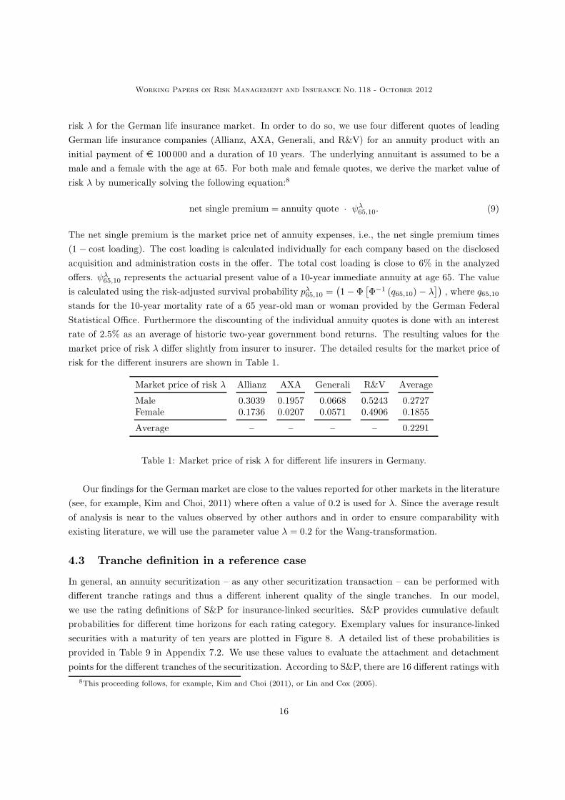
risk for the di!erent insurers are shown in Table 1.
Market price of risk % Allianz AXA Generali R&V Average
Male 0.3039 0.1957 0.0668 0.5243 0.2727Female 0.1736 0.0207 0.0571 0.4906 0.1855
Average – – – – 0.2291
Table 1: Market price of risk % for di!erent life insurers in Germany.
Our findings for the German market are close to the values reported for other markets in the literature
(see, for example, Kim and Choi, 2011) where often a value of 0.2 is used for %. Since the average result
of analysis is near to the values observed by other authors and in order to ensure comparability with
existing literature, we will use the parameter value % = 0.2 for the Wang-transformation.
4.3 Tranche definition in a reference case
In general, an annuity securitization – as any other securitization transaction – can be performed with
di!erent tranche ratings and thus a di!erent inherent quality of the single tranches. In our model,
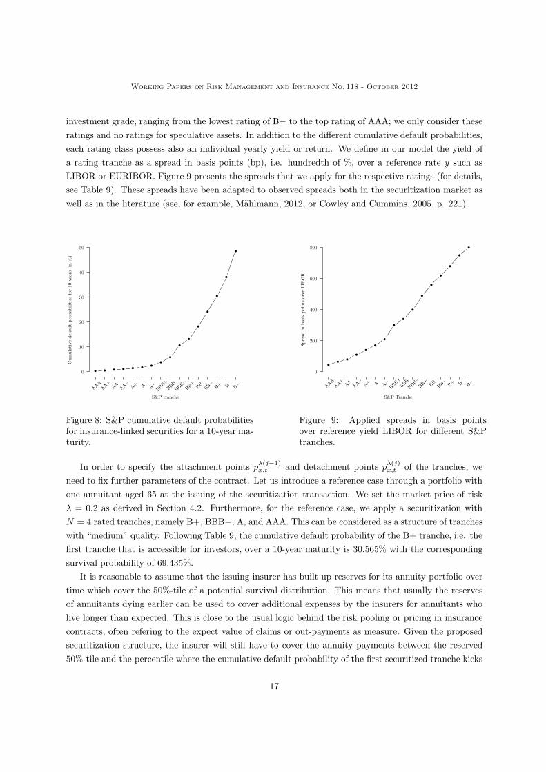
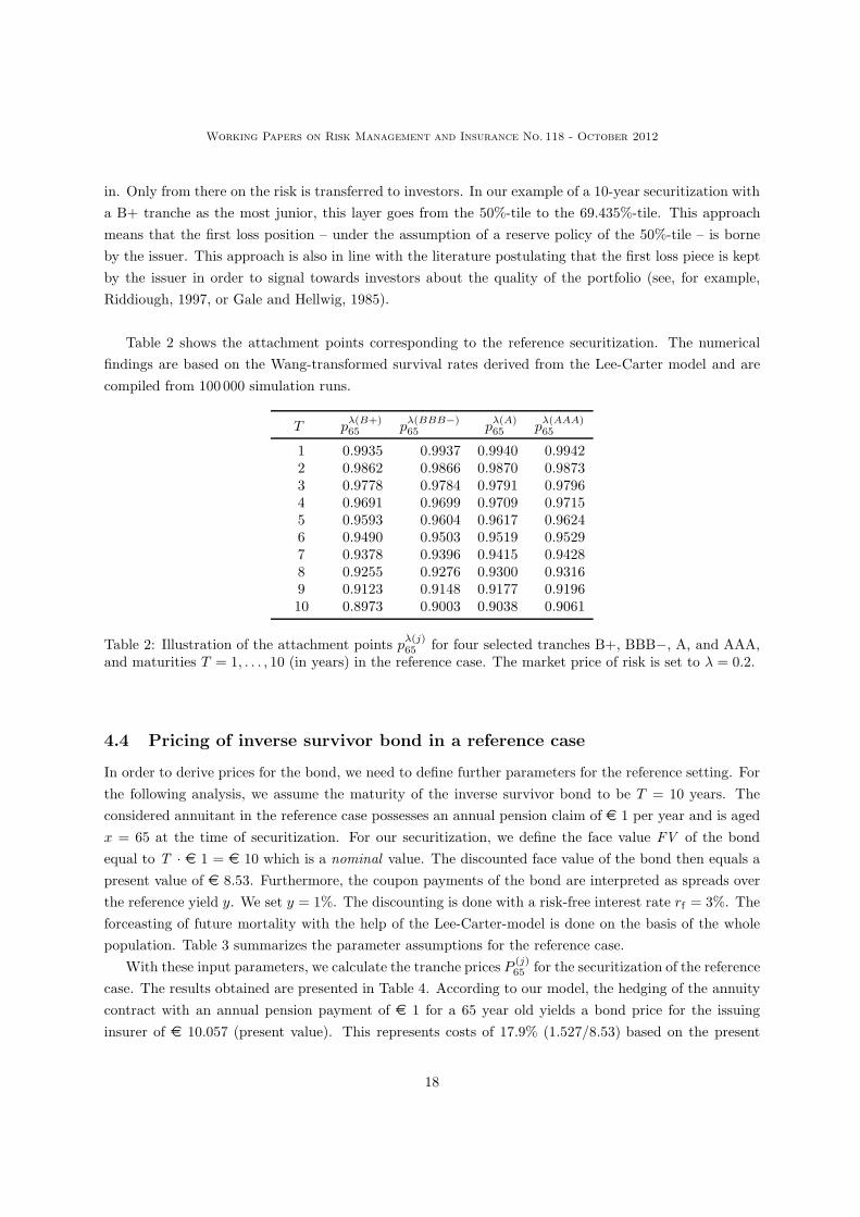
we use the rating definitions of S&P for insurance-linked securities. S&P provides cumulative default
probabilities for di!erent time horizons for each rating category. Exemplary values for insurance-linked
securities with a maturity of ten years are plotted in Figure 8. A detailed list of these probabilities is
provided in Table 9 in Appendix 7.2. We use these values to evaluate the attachment and detachment
points for the di!erent tranches of the securitization. According to S&P, there are 16 di!erent ratings with
8This proceeding follows, for example, Kim and Choi (2011), or Lin and Cox (2005).
16
Working Papers on Risk Management and Insurance No. 118 - October 2012
investment grade, ranging from the lowest rating of B! to the top rating of AAA; we only consider these
ratings and no ratings for speculative assets. In addition to the di!erent cumulative default probabilities,
each rating class possess also an individual yearly yield or return. We define in our model the yield of
a rating tranche as a spread in basis points (bp), i.e. hundredth of %, over a reference rate y such as
LIBOR or EURIBOR. Figure 9 presents the spreads that we apply for the respective ratings (for details,
see Table 9). These spreads have been adapted to observed spreads both in the securitization market as
well as in the literature (see, for example, Mahlmann, 2012, or Cowley and Cummins, 2005, p. 221).
S&P tranche
Cum
ula
tive
def
ault p
robab
ilitie
s fo
r 10
yea
rs (
in %
)
0
10
20
30
40
50
AAAAA+
AAAA!
A+ A A!BBB+
BBBBBB!
BB+BB
BB!B+ B B!
Figure 8: S&P cumulative default probabilitiesfor insurance-linked securities for a 10-year ma-turity.
S&P Tranche
Spre
ad in b
asis
poi
nts
over
LIB
OR
0
200
400
600
800
AAAAA+
AAAA!
A+ A A!BBB+
BBBBBB!
BB+BB
BB!B+ B B!
Figure 9: Applied spreads in basis pointsover reference yield LIBOR for di!erent S&Ptranches.
In order to specify the attachment points p!(j!1)x,t and detachment points p!(j)x,t of the tranches, we
need to fix further parameters of the contract. Let us introduce a reference case through a portfolio with
one annuitant aged 65 at the issuing of the securitization transaction. We set the market price of risk
% = 0.2 as derived in Section 4.2. Furthermore, for the reference case, we apply a securitization with
N = 4 rated tranches, namely B+, BBB!, A, and AAA. This can be considered as a structure of tranches
with “medium” quality. Following Table 9, the cumulative default probability of the B+ tranche, i.e. the
first tranche that is accessible for investors, over a 10-year maturity is 30.565% with the corresponding
survival probability of 69.435%.
It is reasonable to assume that the issuing insurer has built up reserves for its annuity portfolio over
time which cover the 50%-tile of a potential survival distribution. This means that usually the reserves
of annuitants dying earlier can be used to cover additional expenses by the insurers for annuitants who
live longer than expected. This is close to the usual logic behind the risk pooling or pricing in insurance
contracts, often refering to the expect value of claims or out-payments as measure. Given the proposed
securitization structure, the insurer will still have to cover the annuity payments between the reserved
50%-tile and the percentile where the cumulative default probability of the first securitized tranche kicks
17
Working Papers on Risk Management and Insurance No. 118 - October 2012
in. Only from there on the risk is transferred to investors. In our example of a 10-year securitization with
a B+ tranche as the most junior, this layer goes from the 50%-tile to the 69.435%-tile. This approach
means that the first loss position – under the assumption of a reserve policy of the 50%-tile – is borne
by the issuer. This approach is also in line with the literature postulating that the first loss piece is kept
by the issuer in order to signal towards investors about the quality of the portfolio (see, for example,
Riddiough, 1997, or Gale and Hellwig, 1985).
Table 2 shows the attachment points corresponding to the reference securitization. The numerical
findings are based on the Wang-transformed survival rates derived from the Lee-Carter model and are
compiled from 100000 simulation runs.
T p!(B+)65 p!(BBB!)
65 p!(A)65 p!(AAA)
65
1 0.9935 0.9937 0.9940 0.99422 0.9862 0.9866 0.9870 0.98733 0.9778 0.9784 0.9791 0.97964 0.9691 0.9699 0.9709 0.97155 0.9593 0.9604 0.9617 0.96246 0.9490 0.9503 0.9519 0.95297 0.9378 0.9396 0.9415 0.94288 0.9255 0.9276 0.9300 0.93169 0.9123 0.9148 0.9177 0.919610 0.8973 0.9003 0.9038 0.9061
Table 2: Illustration of the attachment points p!(j)65 for four selected tranches B+, BBB!, A, and AAA,and maturities T = 1, . . . , 10 (in years) in the reference case. The market price of risk is set to % = 0.2.
4.4 Pricing of inverse survivor bond in a reference case
In order to derive prices for the bond, we need to define further parameters for the reference setting. For
the following analysis, we assume the maturity of the inverse survivor bond to be T = 10 years. The
considered annuitant in the reference case possesses an annual pension claim of e 1 per year and is aged
x = 65 at the time of securitization. For our securitization, we define the face value FV of the bond
equal to T · e 1 = e 10 which is a nominal value. The discounted face value of the bond then equals a
present value of e 8.53. Furthermore, the coupon payments of the bond are interpreted as spreads over
the reference yield y. We set y = 1%. The discounting is done with a risk-free interest rate rf = 3%. The
forceasting of future mortality with the help of the Lee-Carter-model is done on the basis of the whole
population. Table 3 summarizes the parameter assumptions for the reference case.
With these input parameters, we calculate the tranche prices P (j)65 for the securitization of the reference
case. The results obtained are presented in Table 4. According to our model, the hedging of the annuity
contract with an annual pension payment of e 1 for a 65 year old yields a bond price for the issuing
insurer of e 10.057 (present value). This represents costs of 17.9% (1.527/8.53) based on the present
18
Working Papers on Risk Management and Insurance No. 118 - October 2012
Parameter Variable Value
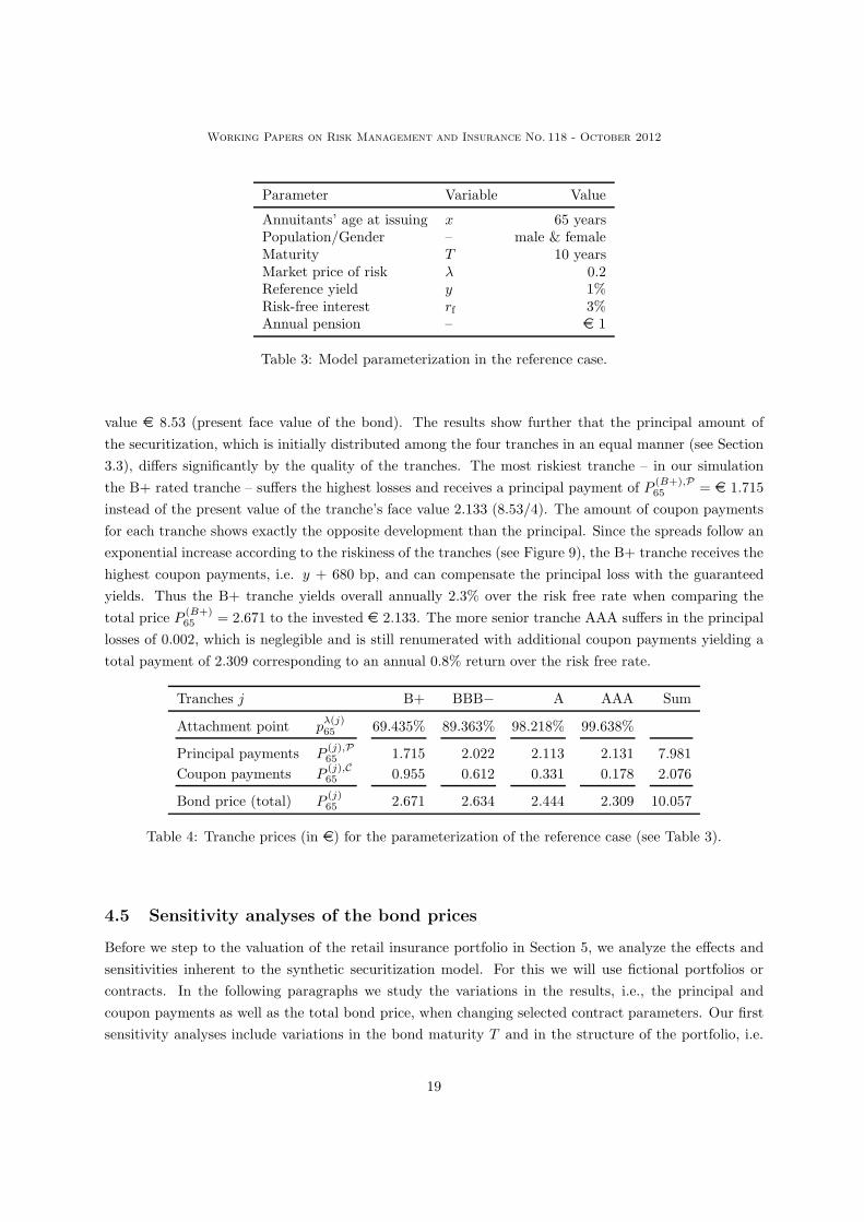
Annuitants’ age at issuing x 65 yearsPopulation/Gender – male & femaleMaturity T 10 yearsMarket price of risk % 0.2Reference yield y 1%Risk-free interest rf 3%Annual pension – e 1
Table 3: Model parameterization in the reference case.
value e 8.53 (present face value of the bond). The results show further that the principal amount of
the securitization, which is initially distributed among the four tranches in an equal manner (see Section
3.3), di!ers significantly by the quality of the tranches. The most riskiest tranche – in our simulation
the B+ rated tranche – su!ers the highest losses and receives a principal payment of P (B+),P65 = e 1.715
instead of the present value of the tranche’s face value 2.133 (8.53/4). The amount of coupon payments
for each tranche shows exactly the opposite development than the principal. Since the spreads follow an
exponential increase according to the riskiness of the tranches (see Figure 9), the B+ tranche receives the
highest coupon payments, i.e. y + 680 bp, and can compensate the principal loss with the guaranteed
yields. Thus the B+ tranche yields overall annually 2.3% over the risk free rate when comparing the
total price P (B+)65 = 2.671 to the invested e 2.133. The more senior tranche AAA su!ers in the principal
losses of 0.002, which is neglegible and is still renumerated with additional coupon payments yielding a
total payment of 2.309 corresponding to an annual 0.8% return over the risk free rate.
Tranches j B+ BBB! A AAA Sum
Attachment point p!(j)65 69.435% 89.363% 98.218% 99.638%
Principal payments P (j),P65 1.715 2.022 2.113 2.131 7.981
Coupon payments P (j),C65 0.955 0.612 0.331 0.178 2.076
Bond price (total) P (j)65 2.671 2.634 2.444 2.309 10.057
Table 4: Tranche prices (in e) for the parameterization of the reference case (see Table 3).
4.5 Sensitivity analyses of the bond prices
Before we step to the valuation of the retail insurance portfolio in Section 5, we analyze the e!ects and
sensitivities inherent to the synthetic securitization model. For this we will use fictional portfolios or
contracts. In the following paragraphs we study the variations in the results, i.e., the principal and
coupon payments as well as the total bond price, when changing selected contract parameters. Our first
sensitivity analyses include variations in the bond maturity T and in the structure of the portfolio, i.e.
19
Working Papers on Risk Management and Insurance No. 118 - October 2012
the rating of the tranches and the number N of tranches. Further analysis include changes in the values
of the reference yield y and of the risk-free interest rf (or discount factor). Finally we also vary the
underlying population considered and its historical mortality rates, i.e., we consider the total (male and
female) population as well as males and females separately.
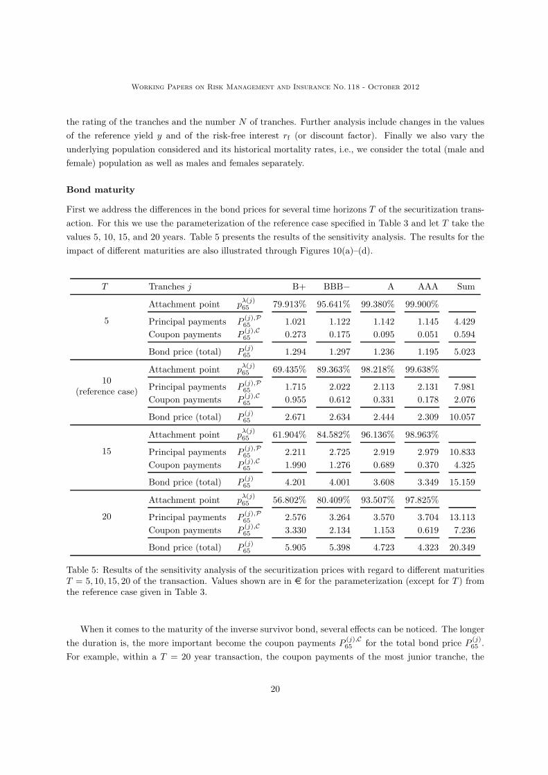
Bond maturity
First we address the di!erences in the bond prices for several time horizons T of the securitization trans-
action. For this we use the parameterization of the reference case specified in Table 3 and let T take the
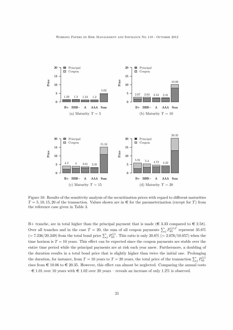
values 5, 10, 15, and 20 years. Table 5 presents the results of the sensitivity analysis. The results for the
impact of di!erent maturities are also illustrated through Figures 10(a)–(d).
T Tranches j B+ BBB! A AAA Sum
5
Attachment point p!(j)65 79.913% 95.641% 99.380% 99.900%
Principal payments P (j),P65 1.021 1.122 1.142 1.145 4.429
Coupon payments P (j),C65 0.273 0.175 0.095 0.051 0.594
Bond price (total) P (j)65 1.294 1.297 1.236 1.195 5.023
10(reference case)
Attachment point p!(j)65 69.435% 89.363% 98.218% 99.638%
Principal payments P (j),P65 1.715 2.022 2.113 2.131 7.981
Coupon payments P (j),C65 0.955 0.612 0.331 0.178 2.076
Bond price (total) P (j)65 2.671 2.634 2.444 2.309 10.057
15
Attachment point p!(j)65 61.904% 84.582% 96.136% 98.963%
Principal payments P (j),P65 2.211 2.725 2.919 2.979 10.833
Coupon payments P (j),C65 1.990 1.276 0.689 0.370 4.325
Bond price (total) P (j)65 4.201 4.001 3.608 3.349 15.159
20
Attachment point p!(j)65 56.802% 80.409% 93.507% 97.825%
Principal payments P (j),P65 2.576 3.264 3.570 3.704 13.113
Coupon payments P (j),C65 3.330 2.134 1.153 0.619 7.236
Bond price (total) P (j)65 5.905 5.398 4.723 4.323 20.349
Table 5: Results of the sensitivity analysis of the securitization prices with regard to di!erent maturitiesT = 5, 10, 15, 20 of the transaction. Values shown are in e for the parameterization (except for T ) fromthe reference case given in Table 3.
When it comes to the maturity of the inverse survivor bond, several e!ects can be noticed. The longer
the duration is, the more important become the coupon payments P (j),C65 for the total bond price P (j)
65 .
For example, within a T = 20 year transaction, the coupon payments of the most junior tranche, the
20
Working Papers on Risk Management and Insurance No. 118 - October 2012
B+ BBB! A AAA Sum
Pri
ce
0
5
10
15
20
B+ BBB! A AAA Sum
Pri
ce
0
5
10
15
20
B+ BBB! A AAA Sum
Pri
ce
0
5
10
15
20
B+ BBB! A AAA Sum
Pri
ce
0
5
10
15
20
B+ BBB! A AAA Sum
Pri
ce
0
5
10
15
20
1.29 1.3 1.24 1.2
5.02
PrincipalCoupon
(a) Maturity T = 5
B+ BBB! A AAA Sum
Pri
ce
0
5
10
15
20
4.2 4 3.61 3.35
15.16
PrincipalCoupon
(c) Maturity T = 15
B+ BBB! A AAA Sum
Pri
ce
0
5
10
15
20
2.67 2.63 2.44 2.31
10.06
PrincipalCoupon
(b) Maturity T = 10
B+ BBB! A AAA Sum
Pri
ce
0
5
10
15
20
5.91 5.4 4.72 4.32
20.35PrincipalCoupon
(d) Maturity T = 20
Figure 10: Results of the sensitivity analysis of the securitization prices with regard to di!erent maturitiesT = 5, 10, 15, 20 of the transaction. Values shown are in e for the parameterization (except for T ) fromthe reference case given in Table 3.
B+ tranche, are in total higher than the principal payment that is made (e 3.33 compared to e 2.58).
Over all tranches and in the case T = 20, the sum of all coupon payments+
j P(j),C65 represent 35.6%
(= 7.236/20.349) from the total bond price+
j P(j)65 . This ratio is only 20.6% (= 2.076/10.057) when the
time horizon is T = 10 years. This e!ect can be expected since the coupon payments are stable over the
entire time period while the principal payments are at risk each year anew. Furthermore, a doubling of
the duration results in a total bond price that is slightly higher than twice the initial one. Prolonging
the duration, for instance, from T = 10 years to T = 20 years, the total price of the transaction+
j P(j)65
rises from e 10.06 to e 20.35. However, this e!ect can almost be neglected. Comparing the annual costs
– e 1.01 over 10 years with e 1.02 over 20 years – reveals an increase of only 1.2% is observed.
21
Working Papers on Risk Management and Insurance No. 118 - October 2012
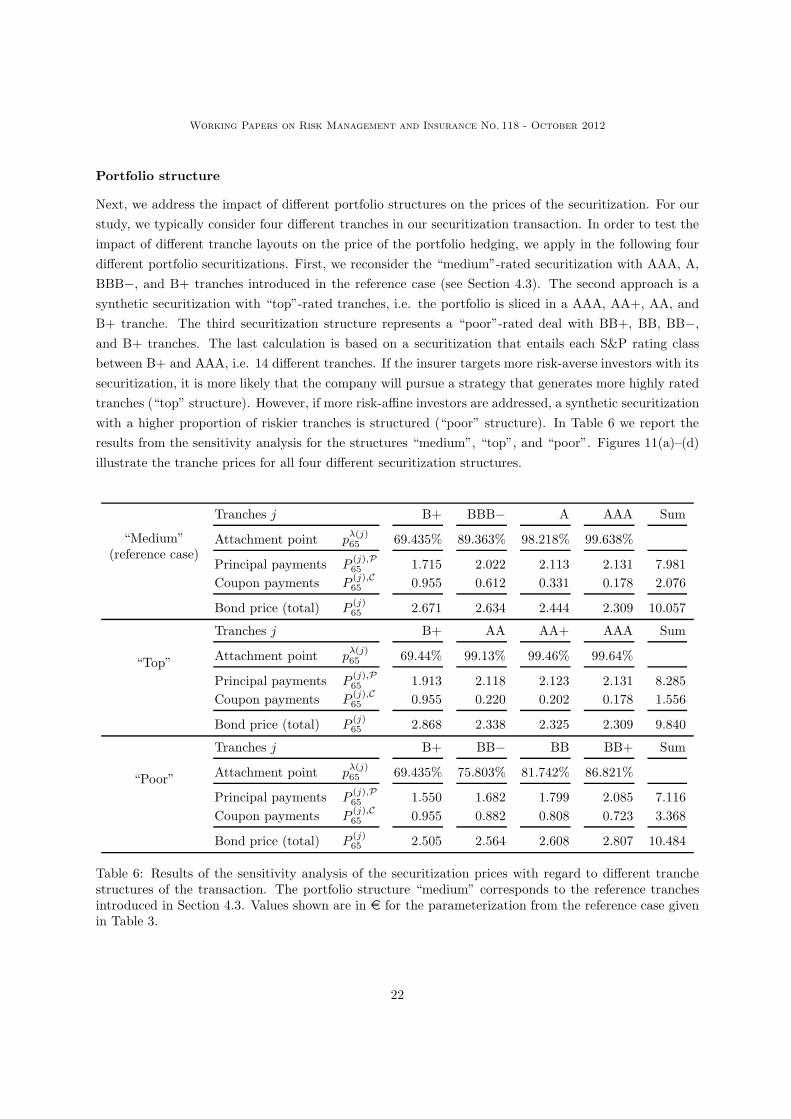
Portfolio structure
Next, we address the impact of di!erent portfolio structures on the prices of the securitization. For our
study, we typically consider four di!erent tranches in our securitization transaction. In order to test the
impact of di!erent tranche layouts on the price of the portfolio hedging, we apply in the following four
di!erent portfolio securitizations. First, we reconsider the “medium”-rated securitization with AAA, A,
BBB!, and B+ tranches introduced in the reference case (see Section 4.3). The second approach is a
synthetic securitization with “top”-rated tranches, i.e. the portfolio is sliced in a AAA, AA+, AA, and
B+ tranche. The third securitization structure represents a “poor”-rated deal with BB+, BB, BB!,
and B+ tranches. The last calculation is based on a securitization that entails each S&P rating class
between B+ and AAA, i.e. 14 di!erent tranches. If the insurer targets more risk-averse investors with its
securitization, it is more likely that the company will pursue a strategy that generates more highly rated
tranches (“top” structure). However, if more risk-a"ne investors are addressed, a synthetic securitization
with a higher proportion of riskier tranches is structured (“poor” structure). In Table 6 we report the
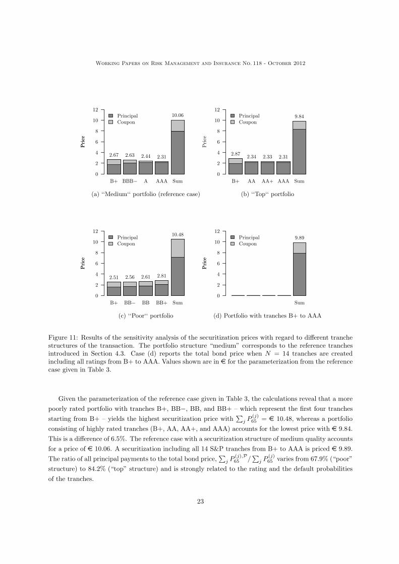
results from the sensitivity analysis for the structures “medium”, “top”, and “poor”. Figures 11(a)–(d)
illustrate the tranche prices for all four di!erent securitization structures.
“Medium”(reference case)
Tranches j B+ BBB! A AAA Sum
Attachment point p!(j)65 69.435% 89.363% 98.218% 99.638%
Principal payments P (j),P65 1.715 2.022 2.113 2.131 7.981
Coupon payments P (j),C65 0.955 0.612 0.331 0.178 2.076
Bond price (total) P (j)65 2.671 2.634 2.444 2.309 10.057
“Top”
Tranches j B+ AA AA+ AAA Sum
Attachment point p!(j)65 69.44% 99.13% 99.46% 99.64%
Principal payments P (j),P65 1.913 2.118 2.123 2.131 8.285
Coupon payments P (j),C65 0.955 0.220 0.202 0.178 1.556
Bond price (total) P (j)65 2.868 2.338 2.325 2.309 9.840
“Poor”
Tranches j B+ BB! BB BB+ Sum
Attachment point p!(j)65 69.435% 75.803% 81.742% 86.821%
Principal payments P (j),P65 1.550 1.682 1.799 2.085 7.116
Coupon payments P (j),C65 0.955 0.882 0.808 0.723 3.368
Bond price (total) P (j)65 2.505 2.564 2.608 2.807 10.484
Table 6: Results of the sensitivity analysis of the securitization prices with regard to di!erent tranchestructures of the transaction. The portfolio structure “medium” corresponds to the reference tranchesintroduced in Section 4.3. Values shown are in e for the parameterization from the reference case givenin Table 3.
22
Working Papers on Risk Management and Insurance No. 118 - October 2012
Pri
ce
0
2
4
6
8
10
12
B+ BBB! A AAA Sum
Pri
ce
0
2
4
6
8
10
12
B+ BB! BB BB+ Sum
0
2
4
6
8
10
12
B+ AA AA+ AAA Sum
Pri
ce
0
2
4
6
8
10
12
Sum
Pri
ce
2.67 2.63 2.44 2.31
10.06PrincipalCoupon
(a) ‘‘Medium‘‘ portfolio (reference case)
Pri
ce
2.51 2.56 2.61 2.81
10.48PrincipalCoupon
(c) ‘‘Poor‘‘ portfolio
Pri
ce
2.872.34 2.33 2.31
9.84PrincipalCoupon
(b) ‘‘Top‘‘ portfolio
Pri
ce
9.89PrincipalCoupon
(d) Portfolio with tranches B+ to AAA
Figure 11: Results of the sensitivity analysis of the securitization prices with regard to di!erent tranchestructures of the transaction. The portfolio structure “medium” corresponds to the reference tranchesintroduced in Section 4.3. Case (d) reports the total bond price when N = 14 tranches are createdincluding all ratings from B+ to AAA. Values shown are in e for the parameterization from the referencecase given in Table 3.
Given the parameterization of the reference case given in Table 3, the calculations reveal that a more
poorly rated portfolio with tranches B+, BB!, BB, and BB+ – which represent the first four tranches
starting from B+ – yields the highest securitization price with+
j P(j)65 = e 10.48, whereas a portfolio
consisting of highly rated tranches (B+, AA, AA+, and AAA) accounts for the lowest price with e 9.84.
This is a di!erence of 6.5%. The reference case with a securitization structure of medium quality accounts
for a price of e 10.06. A securitization including all 14 S&P tranches from B+ to AAA is priced e 9.89.
The ratio of all principal payments to the total bond price,+
j P(j),P65 /
+j P
(j)65 varies from 67.9% (“poor”
structure) to 84.2% (“top” structure) and is strongly related to the rating and the default probabilities
of the tranches.
23
Working Papers on Risk Management and Insurance No. 118 - October 2012
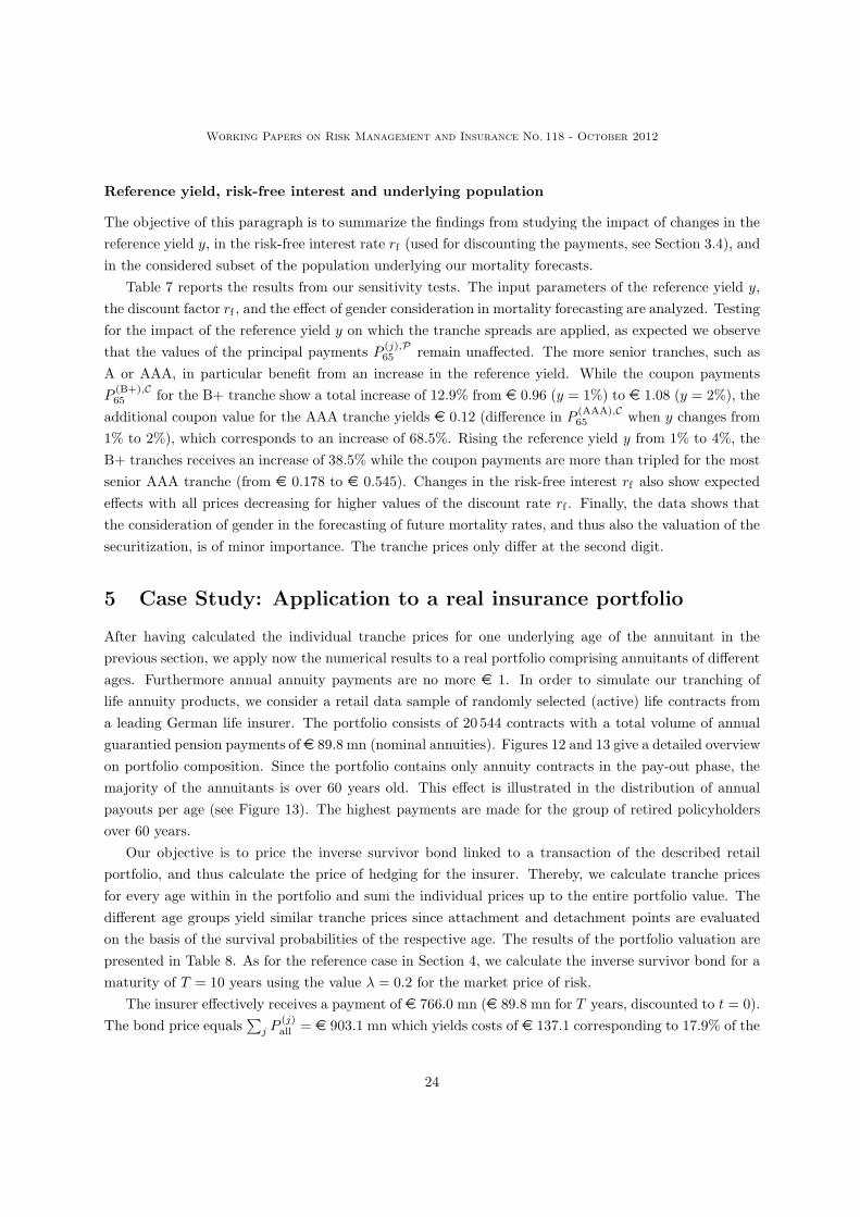
Reference yield, risk-free interest and underlying population
The objective of this paragraph is to summarize the findings from studying the impact of changes in the
reference yield y, in the risk-free interest rate rf (used for discounting the payments, see Section 3.4), and
in the considered subset of the population underlying our mortality forecasts.
Table 7 reports the results from our sensitivity tests. The input parameters of the reference yield y,
the discount factor rf , and the e!ect of gender consideration in mortality forecasting are analyzed. Testing
for the impact of the reference yield y on which the tranche spreads are applied, as expected we observe
that the values of the principal payments P (j),P65 remain una!ected. The more senior tranches, such as
A or AAA, in particular benefit from an increase in the reference yield. While the coupon payments
P (B+),C65 for the B+ tranche show a total increase of 12.9% from e 0.96 (y = 1%) to e 1.08 (y = 2%), the
additional coupon value for the AAA tranche yields e 0.12 (di!erence in P (AAA),C65 when y changes from
1% to 2%), which corresponds to an increase of 68.5%. Rising the reference yield y from 1% to 4%, the
B+ tranches receives an increase of 38.5% while the coupon payments are more than tripled for the most
senior AAA tranche (from e 0.178 to e 0.545). Changes in the risk-free interest rf also show expected
e!ects with all prices decreasing for higher values of the discount rate rf . Finally, the data shows that
the consideration of gender in the forecasting of future mortality rates, and thus also the valuation of the
securitization, is of minor importance. The tranche prices only di!er at the second digit.
5 Case Study: Application to a real insurance portfolio
After having calculated the individual tranche prices for one underlying age of the annuitant in the
previous section, we apply now the numerical results to a real portfolio comprising annuitants of di!erent
ages. Furthermore annual annuity payments are no more e 1. In order to simulate our tranching of
life annuity products, we consider a retail data sample of randomly selected (active) life contracts from
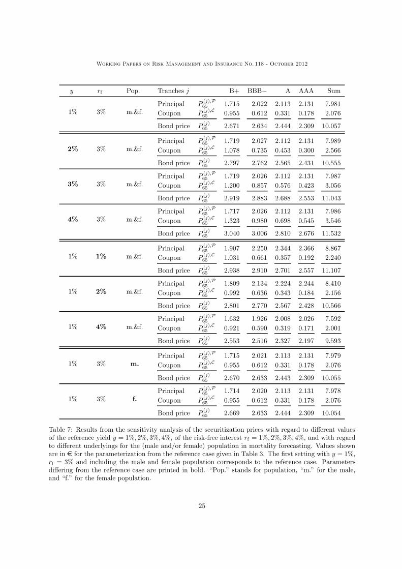
a leading German life insurer. The portfolio consists of 20 544 contracts with a total volume of annual
guarantied pension payments of e 89.8 mn (nominal annuities). Figures 12 and 13 give a detailed overview
on portfolio composition. Since the portfolio contains only annuity contracts in the pay-out phase, the
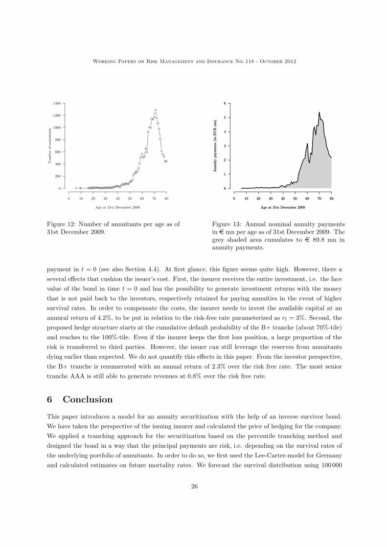
majority of the annuitants is over 60 years old. This e!ect is illustrated in the distribution of annual
payouts per age (see Figure 13). The highest payments are made for the group of retired policyholders
over 60 years.
Our objective is to price the inverse survivor bond linked to a transaction of the described retail
portfolio, and thus calculate the price of hedging for the insurer. Thereby, we calculate tranche prices
for every age within in the portfolio and sum the individual prices up to the entire portfolio value. The
di!erent age groups yield similar tranche prices since attachment and detachment points are evaluated
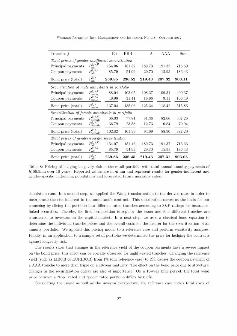
on the basis of the survival probabilities of the respective age. The results of the portfolio valuation are
presented in Table 8. As for the reference case in Section 4, we calculate the inverse survivor bond for a
maturity of T = 10 years using the value % = 0.2 for the market price of risk.
The insurer e!ectively receives a payment of e 766.0 mn (e 89.8 mn for T years, discounted to t = 0).
The bond price equals+
j P(j)all = e 903.1 mn which yields costs of e 137.1 corresponding to 17.9% of the
24
Working Papers on Risk Management and Insurance No. 118 - October 2012
y rf Pop. Tranches j B+ BBB! A AAA Sum
1% 3% m.&f.Principal P (j),P
65 1.715 2.022 2.113 2.131 7.981
Coupon P (j),C65 0.955 0.612 0.331 0.178 2.076
Bond price P (j)65 2.671 2.634 2.444 2.309 10.057
2% 3% m.&f.Principal P (j),P
65 1.719 2.027 2.112 2.131 7.989
Coupon P (j),C65 1.078 0.735 0.453 0.300 2.566
Bond price P (j)65 2.797 2.762 2.565 2.431 10.555
3% 3% m.&f.Principal P (j),P
65 1.719 2.026 2.112 2.131 7.987
Coupon P (j),C65 1.200 0.857 0.576 0.423 3.056
Bond price P (j)65 2.919 2.883 2.688 2.553 11.043
4% 3% m.&f.Principal P (j),P
65 1.717 2.026 2.112 2.131 7.986
Coupon P (j),C65 1.323 0.980 0.698 0.545 3.546
Bond price P (j)65 3.040 3.006 2.810 2.676 11.532
1% 1% m.&f.Principal P (j),P
65 1.907 2.250 2.344 2.366 8.867
Coupon P (j),C65 1.031 0.661 0.357 0.192 2.240
Bond price P (j)65 2.938 2.910 2.701 2.557 11.107
1% 2% m.&f.Principal P (j),P
65 1.809 2.134 2.224 2.244 8.410
Coupon P (j),C65 0.992 0.636 0.343 0.184 2.156
Bond price P (j)65 2.801 2.770 2.567 2.428 10.566
1% 4% m.&f.Principal P (j),P
65 1.632 1.926 2.008 2.026 7.592
Coupon P (j),C65 0.921 0.590 0.319 0.171 2.001
Bond price P (j)65 2.553 2.516 2.327 2.197 9.593
1% 3% m.Principal P (j),P
65 1.715 2.021 2.113 2.131 7.979
Coupon P (j),C65 0.955 0.612 0.331 0.178 2.076
Bond price P (j)65 2.670 2.633 2.443 2.309 10.055
1% 3% f.Principal P (j),P
65 1.714 2.020 2.113 2.131 7.978
Coupon P (j),C65 0.955 0.612 0.331 0.178 2.076
Bond price P (j)65 2.669 2.633 2.444 2.309 10.054
Table 7: Results from the sensitivity analysis of the securitization prices with regard to di!erent valuesof the reference yield y = 1%, 2%, 3%, 4%, of the risk-free interest rf = 1%, 2%, 3%, 4%, and with regardto di!erent underlyings for the (male and/or female) population in mortality forecasting. Values shownare in e for the parameterization from the reference case given in Table 3. The first setting with y = 1%,rf = 3% and including the male and female population corresponds to the reference case. Parametersdi!ering from the reference case are printed in bold. “Pop.” stands for population, “m.” for the male,and “f.” for the female population.
25
Working Papers on Risk Management and Insurance No. 118 - October 2012
Age at 31st December 2009
Num
ber
of an
nuitan
ts
0
200
400
600
800
1000
1200
1400
0 10 20 30 40 50 60 70 80
Figure 12: Number of annuitants per age as of31st December 2009.
Age at 31st December 2009
Annu
ity
pay
men
ts (
in E
UR
mn)
0
1
2
3
4
5
6
0 10 20 30 40 50 60 70 80
Age at 31st December 2009
Annu
ity
pay
men
ts (
in E
UR
mn)
0
1
2
3
4
5
6
0 10 20 30 40 50 60 70 80
Figure 13: Annual nominal annuity paymentsin e mn per age as of 31st December 2009. Thegrey shaded area cumulates to e 89.8 mn inannuity payments.
payment in t = 0 (see also Section 4.4). At first glance, this figure seems quite high. However, there a
several e!ects that cushion the issuer’s cost. First, the insurer receives the entire investment, i.e. the face
value of the bond in time t = 0 and has the possibility to generate investment returns with the money
that is not paid back to the investors, respectively retained for paying annuities in the event of higher
survival rates. In order to compensate the costs, the insurer needs to invest the available capital at an
annural return of 4.2%, to be put in relation to the risk-free rate parameterized as rf = 3%. Second, the
proposed hedge structure starts at the cumulative default probability of the B+ tranche (about 70%-tile)
and reaches to the 100%-tile. Even if the insurer keeps the first loss position, a large proportion of the
risk is transferred to third parties. However, the issuer can still leverage the reserves from annuitants
dying earlier than expected. We do not quantify this e!ects in this paper. From the investor perspective,
the B+ tranche is renumerated with an annual return of 2.3% over the risk free rate. The most senior
tranche AAA is still able to generate revenues at 0.8% over the risk free rate.
6 Conclusion
This paper introduces a model for an annuity securitization with the help of an inverse survivor bond.
We have taken the perspective of the issuing insurer and calculated the price of hedging for the company.
We applied a tranching approach for the securitization based on the percentile tranching method and
designed the bond in a way that the principal payments are risk, i.e. depending on the survival rates of
the underlying portfolio of annuitants. In order to do so, we first used the Lee-Carter-model for Germany
and calculated estimates on future mortality rates. We forecast the survival distribution using 100 000
26
Working Papers on Risk Management and Insurance No. 118 - October 2012
Tranches j B+ BBB! A AAA Sum
Total prices of gender-indi!erent securitization
Principal payments P (j),Pall 154.06 181.52 189.73 191.37 716.69
Coupon payments P (j),Call 85.79 54.99 29.70 15.95 186.43
Bond price (total) P (j)all 239.85 236.52 219.43 207.32 903.11
Securitization of male annuitants in portfolio
Principal payments P (j),Pmale 88.04 103.65 108.37 109.31 409.37
Coupon payments P (j),Cmale 49.00 31.41 16.96 9.11 106.49
Bond price (total) P (j)male 137.04 135.06 125.34 118.42 515.86
Securitization of female annuitants in portfolio
Principal payments P (j),Pfemale 66.03 77.81 81.36 82.06 307.26
Coupon payments P (j),Cfemale 36.79 23.58 12.73 6.84 79.94
Bond price (total) P (j)female 102.82 101.39 94.09 88.90 387.20
Total prices of gender-specific securitization
Principal payments P (j),Pall 154.07 181.46 189.73 191.37 716.63
Coupon payments P (j),Call 85.79 54.99 29.70 15.95 186.43
Bond price (total) P (j)all 239.86 236.45 219.43 207.31 903.05
Table 8: Pricing of hedging longevity risk in the retail portfolio with total annual annuity payments ofe 89.9mn over 10 years. Reported values are in e mn and represent results for gender-indi!erent andgender-specific underlying populations and forecasted future mortality rates.
simulation runs. In a second step, we applied the Wang-transformation to the derived rates in order to
incorporate the risk inherent in the annuitant’s contract. This distribution serves as the basis for our
tranching by slicing the portfolio into di!erent rated tranches according to S&P ratings for insurance-
linked securities. Thereby, the first loss position is kept by the issuer and four di!erent tranches are
transferred to investors on the capital market. In a next step, we used a classical bond equation to
determine the individual tranche prices and the overall costs for the insurer for the securitization of an
annuity portfolio. We applied this pricing model to a reference case and perform sensitivity analyses.
Finally, in an application to a sample retail portfolio we determined the price for hedging the contracts
against longevity risk.
The results show that changes in the reference yield of the coupon payments have a severe impact
on the bond price; this e!ect can be epically observed for highly-rated tranches. Changing the reference
yield (such as LIBOR or EURIBOR) from 1% (our reference case) to 2%, causes the coupon payment of
a AAA tranche to more than triple on a 10-year maturity. The e!ect on the bond price due to structural
changes in the securitization outlay are also of importance. On a 10-year time period, the total bond
price between a “top” rated and “poor” rated portfolio di!ers by 6.5%.
Considering the issuer as well as the investor perspective, the reference case yields total costs of
27

Working Papers on Risk Management and Insurance No. 118 - October 2012
17.9% for the insurer from the securitization. At first, this cost loading seems high; however, due to
the presented structure of the bond, an annual return of 4.2% on the received capital, which the insurer
should invest, is enough to compensate the costs. The transaction is also advantegous for the investors.
Investments into the minor B+ tranche are renumerated with an annual yield of 2.3% over the risk-free
rate, while the most senior AAA tranche – which bears the lowest default risk – still receives annually
0.8% over the risk-free rate.
Our findings contribute to the current discussion about how insurers can face longevity risk within
their annuity portfolios. The fact that the rating structure has such a severe impact on the overall hedging
costs for the insurer implies that companies which are willing to undergo an annuity securitization should
consider their deal structure very carefully. In addition, we have pointed out that in imperfect markets,
the retention of the equity tranche by the originator might be advantageous. Never the less, one has to
bear in mind that by this behavior, the insurer is able to reduce the overall default risk in his balance
sheet by securitizing a life insurance portfolio; however, the fraction of first loss pieces from defaults
increases more than proportionally. The insurer has to take care to not be left with large, unwanted
remaining risk positions in his books.
28
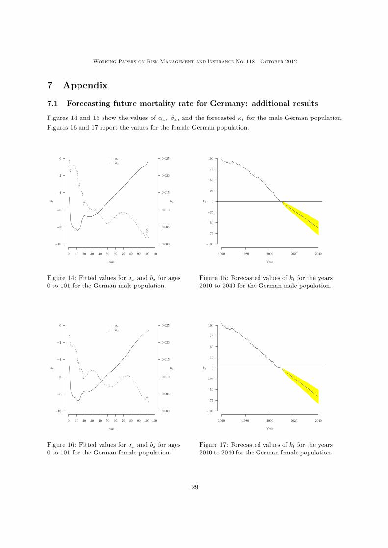
Working Papers on Risk Management and Insurance No. 118 - October 2012
7 Appendix
7.1 Forecasting future mortality rate for Germany: additional results
Figures 14 and 15 show the values of !x, "x, and the forecasted #t for the male German population.
Figures 16 and 17 report the values for the female German population.
!10
!8
!6
!4
!2
0
0.000
0.005
0.010
0.015
0.020
0.025
0 10 20 30 40 50 60 70 80 90 100 110
ax bx
Age
ax
bx
Figure 14: Fitted values for ax and bx for ages0 to 101 for the German male population.
Year
1960 1980 2000 2020 2040
!100
!75
!50
!25
0
25
50
75
100
kt
Figure 15: Forecasted values of kt for the years2010 to 2040 for the German male population.
!10
!8
!6
!4
!2
0
0.000
0.005
0.010
0.015
0.020
0.025
0 10 20 30 40 50 60 70 80 90 100 110
ax bx
Age
ax
bx
Figure 16: Fitted values for ax and bx for ages0 to 101 for the German female population.
Year
1960 1980 2000 2020 2040
!100
!75
!50
!25
0
25
50
75
100
kt
Figure 17: Forecasted values of kt for the years2010 to 2040 for the German female population.
29
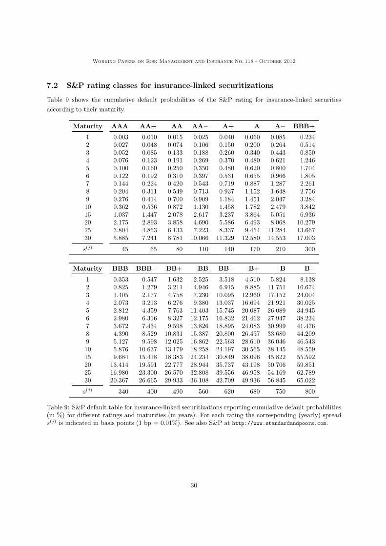
Working Papers on Risk Management and Insurance No. 118 - October 2012
7.2 S&P rating classes for insurance-linked securitizations
Table 9 shows the cumulative default probabilities of the S&P rating for insurance-linked securities
according to their maturity.
Maturity AAA AA+ AA AA! A+ A A! BBB+
1 0.003 0.010 0.015 0.025 0.040 0.060 0.085 0.2342 0.027 0.048 0.074 0.106 0.150 0.200 0.264 0.5143 0.052 0.085 0.133 0.188 0.260 0.340 0.443 0.8504 0.076 0.123 0.191 0.269 0.370 0.480 0.621 1.2465 0.100 0.160 0.250 0.350 0.480 0.620 0.800 1.7046 0.122 0.192 0.310 0.397 0.531 0.655 0.966 1.8057 0.144 0.224 0.420 0.543 0.719 0.887 1.287 2.2618 0.204 0.311 0.549 0.713 0.937 1.152 1.648 2.7569 0.276 0.414 0.700 0.909 1.184 1.451 2.047 3.28410 0.362 0.536 0.872 1.130 1.458 1.782 2.479 3.84215 1.037 1.447 2.078 2.617 3.237 3.864 5.051 6.93620 2.175 2.893 3.858 4.690 5.586 6.493 8.068 10.27925 3.804 4.853 6.133 7.223 8.337 9.454 11.284 13.66730 5.885 7.241 8.781 10.066 11.329 12.580 14.553 17.003
s(j) 45 65 80 110 140 170 210 300
Maturity BBB BBB! BB+ BB BB! B+ B B!
1 0.353 0.547 1.632 2.525 3.518 4.510 5.824 8.1382 0.825 1.279 3.211 4.946 6.915 8.885 11.751 16.6743 1.405 2.177 4.758 7.230 10.095 12.960 17.152 24.0044 2.073 3.213 6.276 9.380 13.037 16.694 21.921 30.0255 2.812 4.359 7.763 11.403 15.745 20.087 26.089 34.9456 2.980 6.316 8.327 12.175 16.832 21.462 27.947 38.2347 3.672 7.434 9.598 13.826 18.895 24.083 30.999 41.4768 4.390 8.529 10.831 15.387 20.800 26.457 33.680 44.2099 5.127 9.598 12.025 16.862 22.563 28.610 36.046 46.54310 5.876 10.637 13.179 18.258 24.197 30.565 38.145 48.55915 9.684 15.418 18.383 24.234 30.849 38.096 45.822 55.59220 13.414 19.591 22.777 28.944 35.737 43.198 50.706 59.85125 16.980 23.300 26.570 32.808 39.556 46.958 54.169 62.78930 20.367 26.665 29.933 36.108 42.709 49.936 56.845 65.022
s(j) 340 400 490 560 620 680 750 800
Table 9: S&P default table for insurance-linked securitizations reporting cumulative default probabilities(in %) for di!erent ratings and maturities (in years). For each rating the corresponding (yearly) spreads(j) is indicated in basis points (1 bp = 0.01%). See also S&P at http://www.standardandpoors.com.
30

Working Papers on Risk Management and Insurance No. 118 - October 2012
References
Bae, T., C. Kim, and R. J. Kulperger, 2009, Securitization of Motor Insurance Loss Rate Risks, Insurance:
Mathematics and Economics, 44(1):48–58.
Bauer, D., M. Borger, and J. Ruß, 2010, On the Pricing of Longevity-Linked Securities, Insurance:
Mathematics and Economics, 46(1):139–149.
Beltratti, A. and G. Corvino, 2008, Why are Insurance Companies Di!erent? The Limits of Conver-
gence Among Financial Institutions, The Geneva Papers on Risk and Insurance Issues and Practice,
33(3):363–388.
Bi"s, E. and D. Blake, 2010, Securitizing and Tranching Longevity Exposures, Insurance: Mathematics
and Economics, 46(1):186–197.
Blake, D., 2003, Reply to ”Survivor Bonds: A Comment on Blake and Burrows”, The Journal of Risk
and Insurance, 70(2):349–351.
Blake, D. and W. Burrows, 2001, Survivor Bonds: Helping to Hedge Mortality Risk, The Journal of Risk
and Insurance, 68(2):339–348.
Blake, D., A. Cairns, K. Dowd, and R. Macminn, 2006, Longevity Bonds: Financial Engineering, Valua-
tion, and Hedging, The Journal of Risk and Insurance, 73(4):647–672.
Blake, D., C. Courbage, R. MacMinn, and M. Sherris, 2011, Longevity Risk and Capital Markets: The
2010/2011 Update, The Geneva Papers on Risk and Insurance Issues and Practice, 36(4):489–500.
Booth, H. and L. Tickle, 2008, Mortality Modelling and Forecasting : A Review of Methods, Annals of
Actuarial Science, 1(2):3–43.
Cairns, A. J. G., D. Blake, and K. Dowd, 2006, A Two-Factor Model for Stochastic Mortality with
Parameter Uncertainty: Theory and Calibration, The Journal of Risk and Insurance, 73(4):687–718.
Chen, B., L. Zhang, and L. Zhao, 2010, On The Robustness of Longevity Risk Pricing, Insurance:
Mathematics and Economics, 47(3):358–373.
Chen, H. and J. D. Cummins, 2010, Longevity Bond Premiums: The Extreme Value Approach and Risk
Cubic Pricing, Insurance: Mathematics and Economics, 46(1):150–161.
Cowley, A. and J. D. Cummins, 2005, Securitization of Life Insurance Assets and Liabilities, The Journal
of Risk and Insurance, 72(2):193–226.
Cox, S. H. and Y. Lin, 2007, Natural Hedging of Life and Annuity Mortality Risk, North American
Actuarial Journal, 11(3):1–15.
Cox, S. H., Y. Lin, and H. Pedersen, 2010, Mortality risk modeling: Applications to insurance securiti-
zation, Insurance: Mathematics and Economics, 46(1):242–253.
31

Working Papers on Risk Management and Insurance No. 118 - October 2012
Cox, S. H., Y. Lin, and S. Wang, 2006, Multivariate Exponential Tilting and Pricing Implications for
Mortality Securitization, The Journal of Risk and Insurance, 73(4):719–736.
Cox, S. H. and R. G. Schwebach, 1992, Insurance Futures and Hedging Insurance Price Risk, The Journal
of Risk and Insurance, 59(4):628–644.
Cummins, J. D. and P. Trainar, 2009, Securitization, Insurance, and Reinsurance, The Journal of Risk
and Insurance, 76(3):463–492.
Cummins, J. D. and M. A. Weiss, 2009, Convergence of Insurance and Financial Markets: Hybrid and
Securitized Risk-Transfer Solutions, The Journal of Risk and Insurance, 76(3):493–545.
Czado, C., A. Delwarde, and M. Denuit, 2005, Bayesian Poisson Log-Bilinear Mortality Projections,
Insurance: Mathematics and Economics, 36(3):260–284.
D’Arcy, S. P. and V. G. France, 1992, Catastrophe Futures : A Better Hedge for Insurers, The Journal
of Risk and Insurance, 59(4):575–600.
De Jong, P. and L. Tickle, 2006, Mathematical Population Studies Extending Lee-Carter Mortality
Forecasting, Mathematical Population Studies, 13(1):1–18.
De Mey, J., 2007, Insurance and the Capital Markets, The Geneva Papers on Risk and Insurance Issues
and Practice, 32(1):35–41.
Delwarde, A., M. Denuit, and P. Eilers, 2007, Smoothing the Lee-Carter and Poisson Log-Bilinear Models
for Mortality Forecasting : a Penalized Log-Likelihood Approach, Statistical Modelling, 7(1):29–48.
Deng, Y., P. L. Brockett, and R. D. MacMinn, 2012, Longevity/Mortality Risk Modeling and Securities
Pricing, The Journal of Risk and Insurance, 79(3):697–721.
Denuit, M., P. Devolder, and A.-C. Goderniaux, 2007, Securitization of Longevity Risk: Pricing Sur-
vivor Bonds With Wang Transform in the Lee-Carter Framework, The Journal of Risk and Insurance,
74(1):87–113.
Deutsche Bank, 2010, Insurance-Linked Securities – A Niche Market Expanding, Research Report.
Dowd, K., 2003, Survivor Bonds: A Comment on Blake and Burrows, The Journal of Risk and Insurance,
70(2):339–348.
Dowd, K., D. Blake, A. J. G. Cairns, and P. Dawson, 2006, Survivor Swaps, The Journal of Risk and
Insurance, 73(1):1–17.
Gale, D. and M. Hellwig, 1985, Incentive-Compatible Debt Contracts : The One-Period Problem, The
Review of Economic Studies, 52(4):647–663.
Gatzert, N. and H. Wesker, 2012, The Impact of Natural Hedging on a Life Insurer’s Risk Situation,
Journal of Risk Finance, (forthcoming).
32

Working Papers on Risk Management and Insurance No. 118 - October 2012
Hanewald, K., T. Post, and H. Grundl, 2011, Stochastic Mortality, Macroeconomic Risks and Life Insurer
Solvency, The Geneva Papers on Risk and Insurance Issues and Practice, 36(3):458–475.
Kampa, C., 2010, Alternative Risk Transfer: The Convergence of The Insurance and Capital Markets.
Part III, Insurance Studies Institute, (available at http://www.ssrn.com).
Kim, C. and Y. Choi, 2011, Securitization of Longevity Risk Using Percentile Tranching, The Journal of
Risk and Insurance, 78(4):885–906.
Lane, M. N. and R. G. Beckwith, 2007, That was the Year that was! The 2007 Review of the Insurance
Securitization Market, Lane Financial L.L.C., (available at http://www.lanefinancialllc.com).
Lee, R. and T. Miller, 2001, Evaluating the Performance of the Lee-Carter Method for Forecasting
Mortality, Demography, 38(4):537–549.
Lee, R. D. and L. R. Carter, 1992, Modeling and Forecasting U. S. Mortality, Journal of the American
Statistical Association, 87(419):659–671.
Lin, Y. and S. H. Cox, 2005, Securitization of Mortality Risks in Life Annuities, The Journal of Risk and
Insurance, 72(2):227–252.
Lin, Y. and S. H. Cox, 2008, Securitization of Catastrophe Mortality Risks, Insurance: Mathematics and
Economics, 42(2):628–637.
Litzenberger, R. H., D. R. Beaglehole, and C. E. Reynolds, 1996, Assessing Catastrophe Reinsurance-
Linked Securities as a New Asset Class, Journal of Portfolio Management, 23:76–86.
Lorson, J., 2012, The Impact of Life Insurance Securitization on the Issuer’s Default Risk, Working Paper
on Risk Management and Insurance (I.VW-HSG).
Luciano, E., L. Regis, and E. Vigna, 2012, DeltaGamma Hedging of Mortality and Interest Rate Risk,
Insurance: Mathematics and Economics, 50(3):402–412.
MacDonald, A., A. J. Cairns, P. L. Gwilt, and K. A. Miller, 1998, An International Comparison of Recent
Trends in Population Mortality, British Actuarial Journal, 4(1):3–141.
Mahlmann, T., 2012, Did Investors Outsource Their Risk Analysis to Rating Agencies? Evidence from
ABS-CDOs, Journal of Banking & Finance, 36(5):1478–1491.
Renshaw, A. E. and S. Haberman, 2006, A Cohort-Based Extension to the Lee-Carter Model for Mortality
Reduction Factors, Insurance: Mathematics and Economics, 38(3):556–570.
Riddiough, T., 1997, Optimal Design and Governance of Asset-Backed Securities, Journal of Financial
Intermediation, 6(2):121–152.
Swiss Re, 2006, Securitization New Opportunities for Insurers and Investors, Technical Report, Swiss
Re, Zurich.
33
Working Papers on Risk Management and Insurance No. 118 - October 2012
Wang, J. L., M.-h. Hsieh, and Y.-f. Chiu, 2011, Using Reverse Mortgages to Hedge Longevity and
Financial Risks for Life Insurers: A Generalised Immunisation Approach, The Geneva Papers on Risk
and Insurance Issues and Practice, 36(4):697–717.
Wang, J. L., H. Huang, S. S. Yang, and J. T. Tsai, 2010, An Optimal Product Mix for Hedging Longevity
Risk in Life Insurance Companies: The Immunization Theory Approach, The Journal of Risk and
Insurance, 77(2):473–497.
Wang, S. S., 2000, A Class of Distortion Operators for Pricing Financial and Insurance Risks, The Journal
of Risk and Insurance, 67(1):15–36.
Wills, S. and M. Sherris, 2010, Securitization, Structuring and Pricing of Longevity Risk, Insurance:
Mathematics and Economics, 46(1):173–185.
34