Embed Size (px)
Citation preview
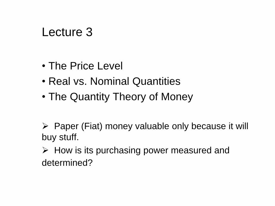
Lecture 3
• The Price Level
• Real vs. Nominal Quantities
• The Quantity Theory of Money
F11
Lecture 3
• The Price Level
• Real vs. Nominal Quantities
• The Quantity Theory of Money
Paper (Fiat) money valuable only because it will
buy stuff.
How is its purchasing power measured and
determined?
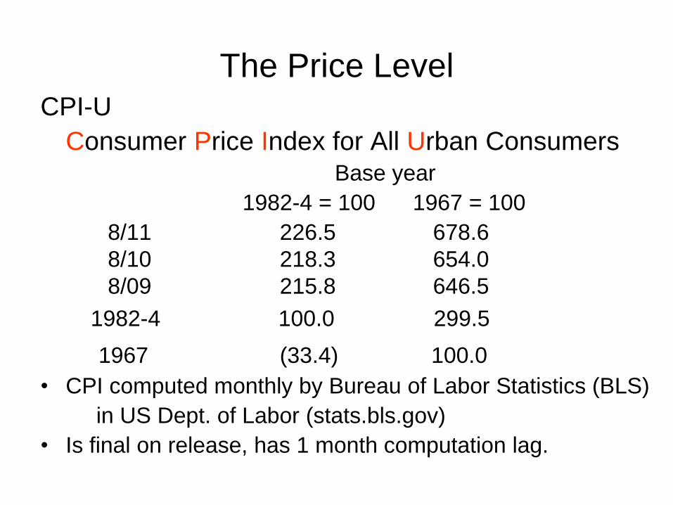
The Price Level CPI-U
Consumer Price Index for All Urban Consumers Base year
1982-4 = 100 1967 = 100
8/11 226.5 678.6
8/10 218.3 654.0
8/09 215.8 646.5
1982-4 100.0 299.5
1967 (33.4) 100.0
• CPI computed monthly by Bureau of Labor Statistics (BLS)
in US Dept. of Labor (stats.bls.gov)
• Is final on release, has 1 month computation lag.
0
50
100
150
200
250
1950 1960 1970 1980 1990 2000 2010
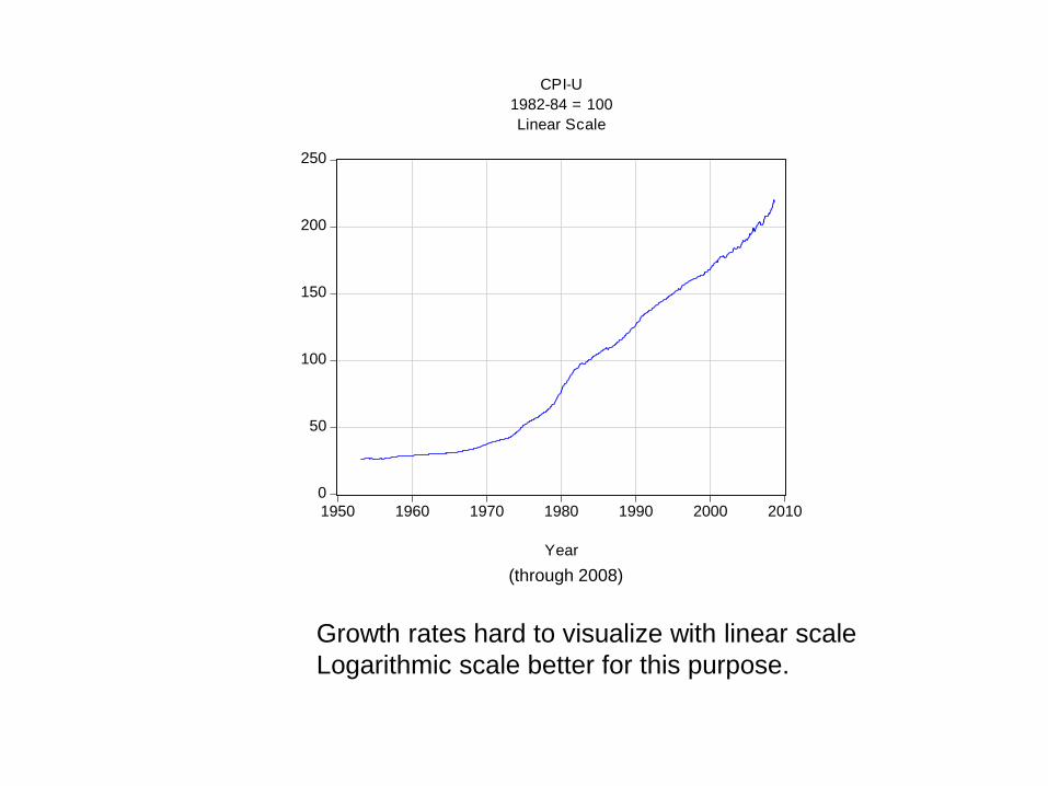
CPI-U
1982-84 = 100
Linear Scale
Year
Growth rates hard to visualize with linear scale
Logarithmic scale better for this purpose.
(through 2008)
200
160
120
100
80
60
40
20
1950 1960 1970 1980 1990 2000 2010
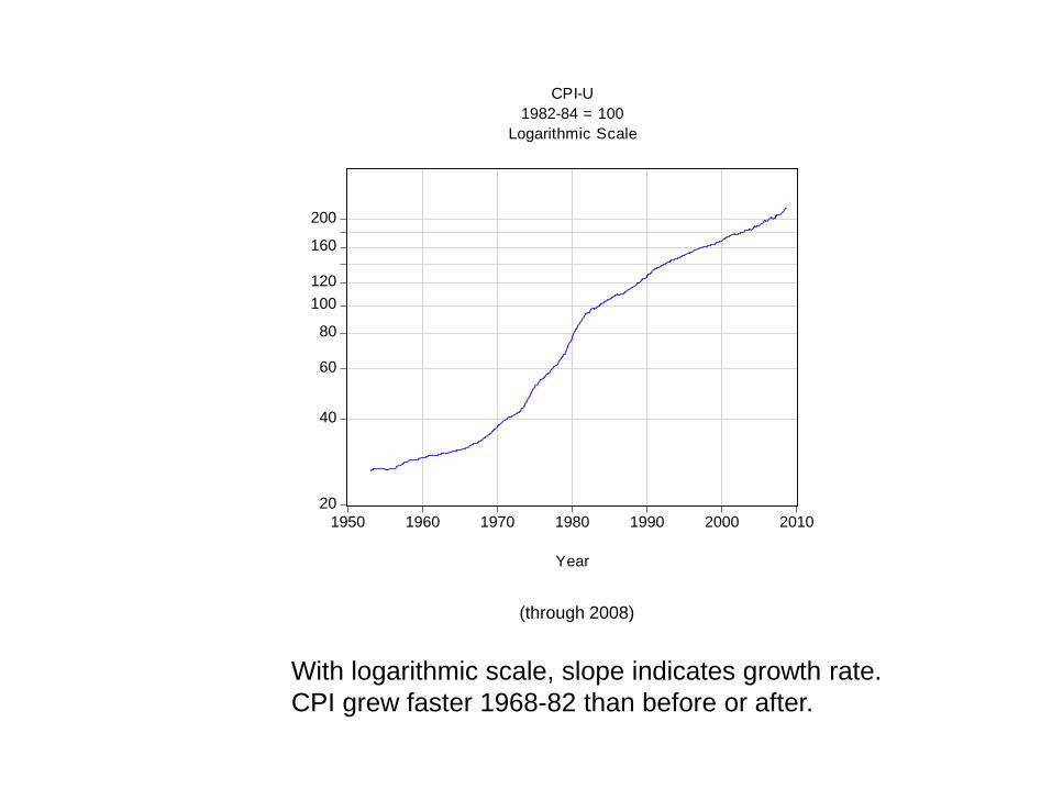
CPI-U
1982-84 = 100
Logarithmic Scale
Year
With logarithmic scale, slope indicates growth rate.
CPI grew faster 1968-82 than before or after.
(through 2008)
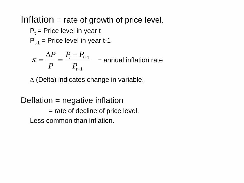
Inflation = rate of growth of price level.
Pt = Price level in year t
Pt-1 = Price level in year t-1
= annual inflation rate
(Delta) indicates change in variable.
Deflation = negative inflation
= rate of decline of price level.
Less common than inflation.
1
1
t
tt
P
PP
P
P
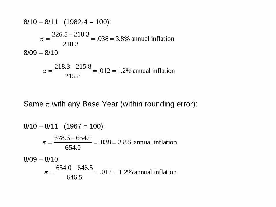
8/10 – 8/11 (1982-4 = 100):
8/09 – 8/10:
Same with any Base Year (within rounding error):
8/10 – 8/11 (1967 = 100):
8/09 – 8/10:
inflation annual %8.3038.3.218
3.2185.226
inflation annual %8.3038.0.654
0.6546.678
inflation annual %2.1012.8.215
8.2153.218
inflation annual %2.1012.5.646
5.6460.654
-10
-5
0
5
10
15
20
25
1950 1960 1970 1980 1990 2000 2010
Year
Perc
ent
per
annum
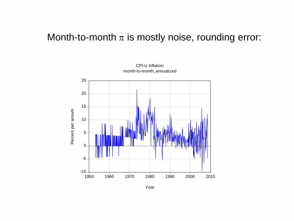
CPI-U Inflation
month-to-month, annualized
Month-to-month is mostly noise, rounding error:
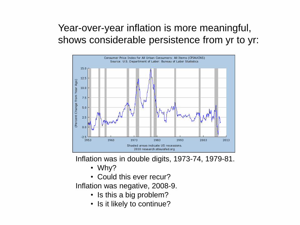
Year-over-year inflation is more meaningful,
shows considerable persistence from yr to yr:
Inflation was in double digits, 1973-74, 1979-81.
• Why?
• Could this ever recur?
Inflation was negative, 2008-9.
• Is this a big problem?
• Is it likely to continue?
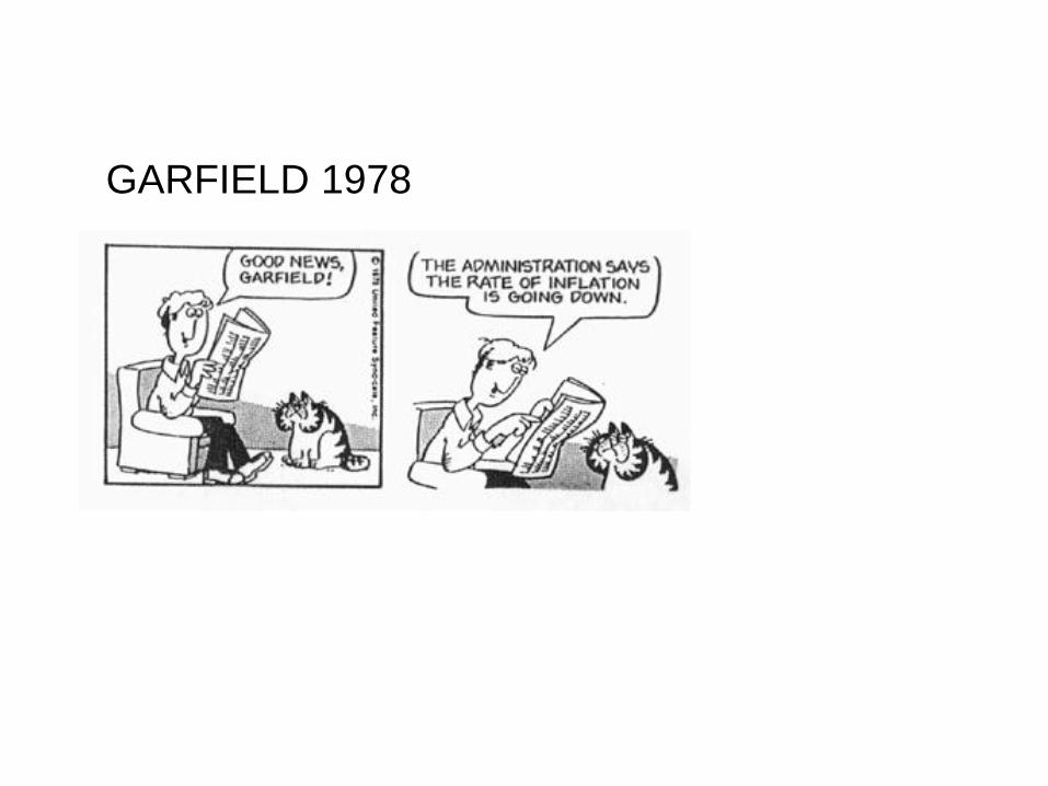
GARFIELD 1978
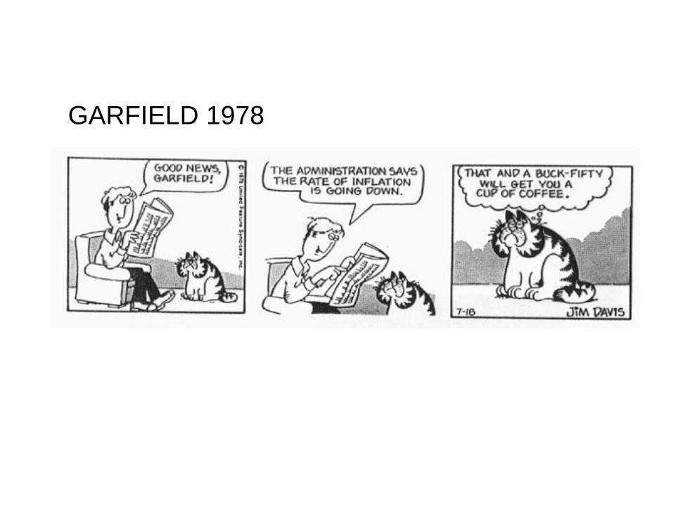
GARFIELD 1978
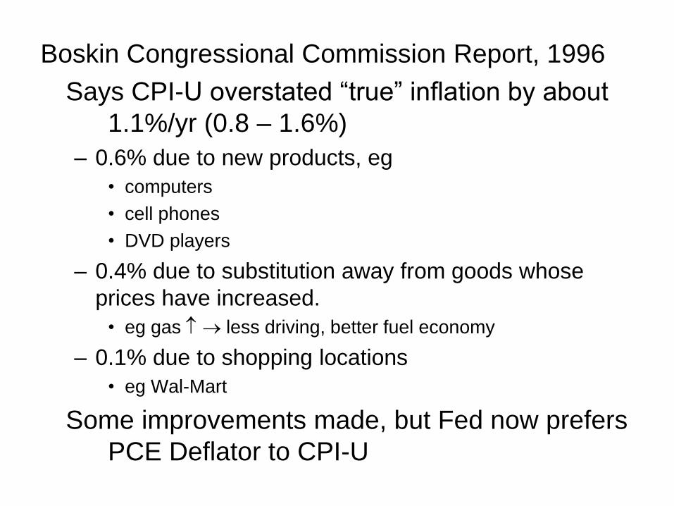
Boskin Congressional Commission Report, 1996
Says CPI-U overstated “true” inflation by about
1.1%/yr (0.8 – 1.6%)
– 0.6% due to new products, eg
• computers
• cell phones
• DVD players
– 0.4% due to substitution away from goods whose
prices have increased.
• eg gas less driving, better fuel economy
– 0.1% due to shopping locations
• eg Wal-Mart
Some improvements made, but Fed now prefers
PCE Deflator to CPI-U
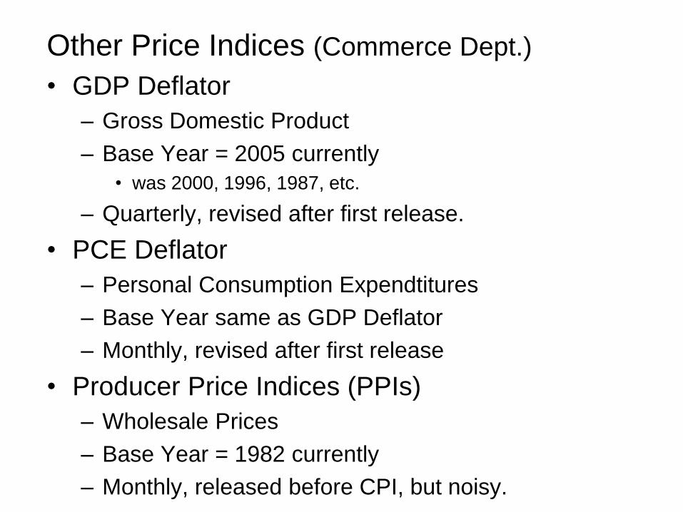
Other Price Indices (Commerce Dept.)
• GDP Deflator
– Gross Domestic Product
– Base Year = 2005 currently
• was 2000, 1996, 1987, etc.
– Quarterly, revised after first release.
• PCE Deflator
– Personal Consumption Expendtitures
– Base Year same as GDP Deflator
– Monthly, revised after first release
• Producer Price Indices (PPIs)
– Wholesale Prices
– Base Year = 1982 currently
– Monthly, released before CPI, but noisy.
300
200
100
80
60
50
40
30
20
1950 1960 1970 1980 1990 2000 2010
YEAR
CPI-U
GDP DEF
PCE DEF
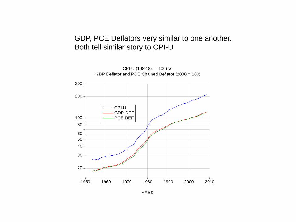
CPI-U (1982-84 = 100) vs
GDP Deflator and PCE Chained Deflator (2000 = 100)
GDP, PCE Deflators very similar to one another.
Both tell similar story to CPI-U
0
1
2
3
4
5
6
7
1980 1985 1990 1995 2000 2005 2010
YEAR
CPI-U
PCE
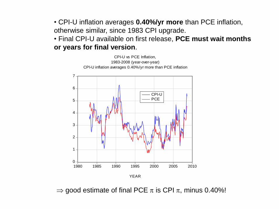
CPI-U vs PCE Inflation,
1983-2008 (year-over-year)
CPI-U inflation averages 0.40%/yr more than PCE inflation
• CPI-U inflation averages 0.40%/yr more than PCE inflation,
otherwise similar, since 1983 CPI upgrade.
• Final CPI-U available on first release, PCE must wait months
or years for final version.
good estimate of final PCE is CPI , minus 0.40%!
200
160
120
100
80
60
40
20
1950 1960 1970 1980 1990 2000 2010
YEAR
CPI-U
PPI All
PPI FCG
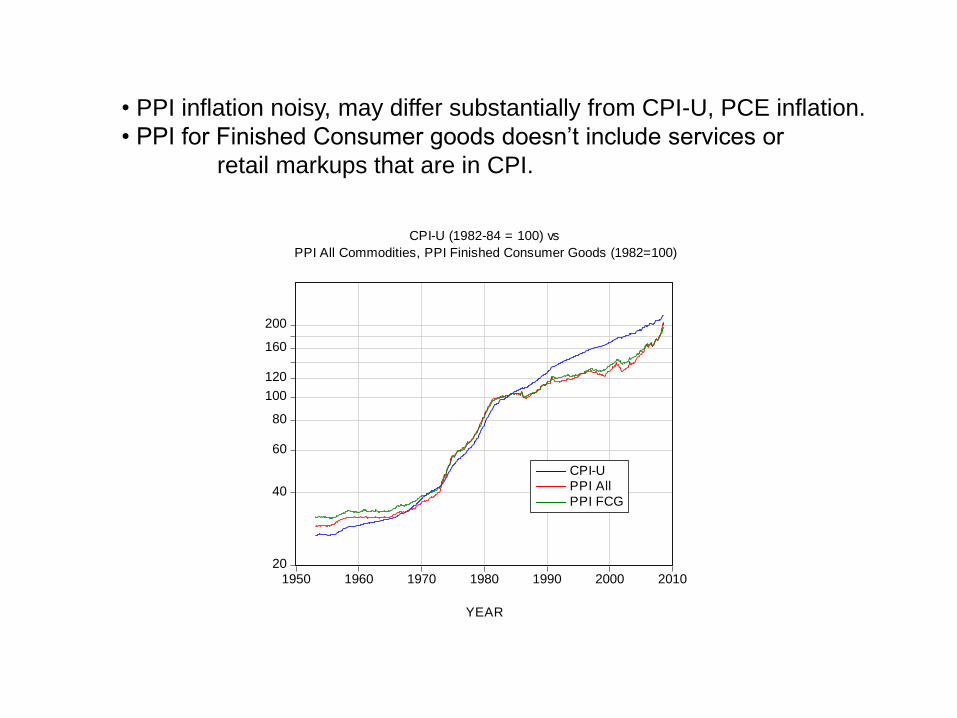
CPI-U (1982-84 = 100) vs
PPI All Commodities, PPI Finished Consumer Goods (1982=100)
• PPI inflation noisy, may differ substantially from CPI-U, PCE inflation.
• PPI for Finished Consumer goods doesn’t include services or
retail markups that are in CPI.
Real vs. Nominal Quantities
Nominal – Current (year t) $
Real – Base year (year t0) $
Pt = Price Index
Yt = Nominal Income (upper case)
yt = Yt · P0 / Pt = Real Income (lower case)
(in year t0 $)
To simplify, we often take P0 = 1.00. Then,
yt = Yt / Pt or y = Y / P
Similarly, if Mt = Nominal Money Stock (upper case),
mt = Mt / Pt = M / P = Real Money Stock (lower case).
20.0
14.0
10.0
6.0
4.0
2.0
1.4
1.0
0.6
0.4
0.2
1950 1960 1970 1980 1990 2000 2010
YEAR
Nominal GDP
Real GDP
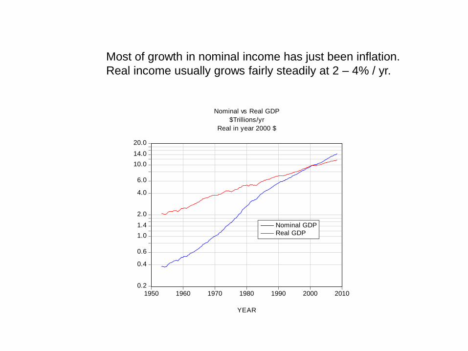
Nominal vs Real GDP
$Trillions/yr
Real in year 2000 $
Most of growth in nominal income has just been inflation.
Real income usually grows fairly steadily at 2 – 4% / yr.
0
1
2
3
4
5
6
7
8
1950 1960 1970 1980 1990 2000 2010
YEAR
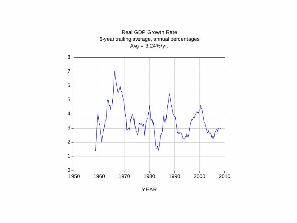
Real GDP Growth Rate
5-year trailing average, annual percentages
Avg = 3.24%/yr.
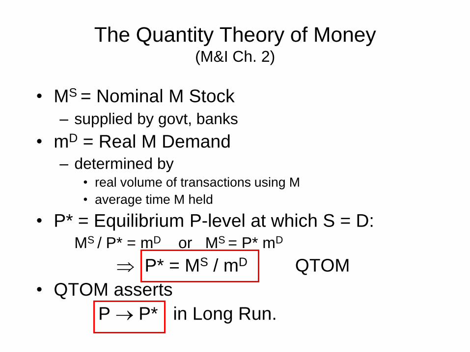
The Quantity Theory of Money (M&I Ch. 2)
• MS = Nominal M Stock – supplied by govt, banks
• mD = Real M Demand – determined by
• real volume of transactions using M
• average time M held
• P* = Equilibrium P-level at which S = D: MS / P* = mD or MS = P* mD
P* = MS / mD QTOM
• QTOM asserts
P P* in Long Run.
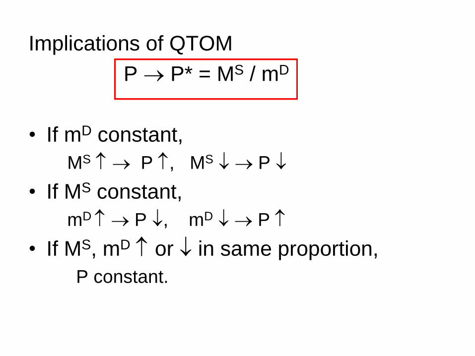
Implications of QTOM
P P* = MS / mD
• If mD constant,
MS P , MS P
• If MS constant,
mD P , mD P
• If MS, mD or in same proportion,
P constant.
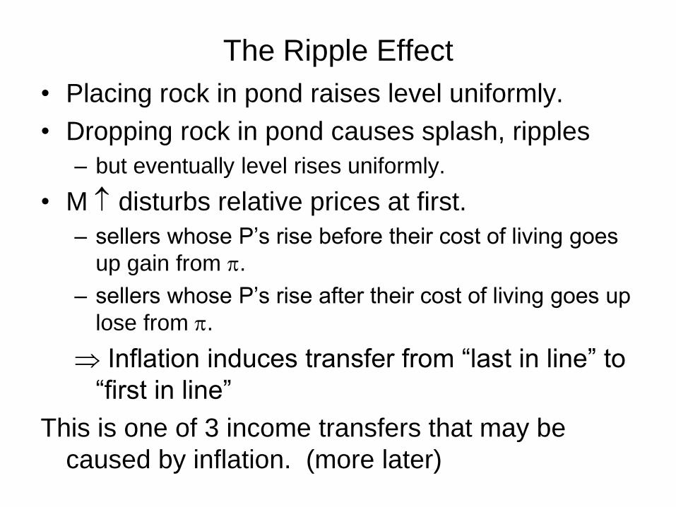
The Ripple Effect
• Placing rock in pond raises level uniformly.
• Dropping rock in pond causes splash, ripples
– but eventually level rises uniformly.
• M disturbs relative prices at first.
– sellers whose P’s rise before their cost of living goes
up gain from .
– sellers whose P’s rise after their cost of living goes up
lose from .
Inflation induces transfer from “last in line” to
“first in line”
This is one of 3 income transfers that may be
caused by inflation. (more later)
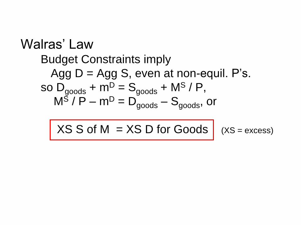
Walras’ Law Budget Constraints imply
Agg D = Agg S, even at non-equil. P’s.
so Dgoods + mD = Sgoods + MS / P,
MS / P – mD = Dgoods – Sgoods, or
XS S of M = XS D for Goods (XS = excess)
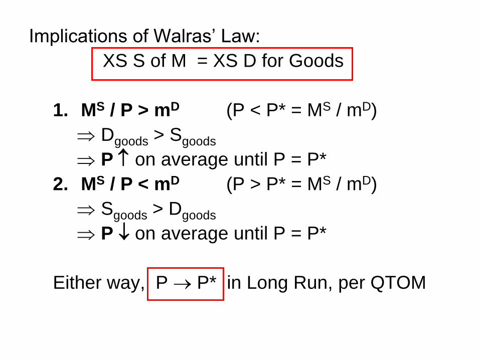
Implications of Walras’ Law:
XS S of M = XS D for Goods
1. MS / P > mD (P < P* = MS / mD)
Dgoods > Sgoods
P on average until P = P*
2. MS / P < mD (P > P* = MS / mD)
Sgoods > Dgoods
P on average until P = P*
Either way, P P* in Long Run, per QTOM
• HW 2 due Fri 5 PM.
• Next:
– Interest rates: nominal vs. real
– M&B 6, 8, 19 pp. 1-3,
– M&I 4.1, 7.1