Embed Size (px)
Citation preview

The Price Effects of Cross-Market Hospital Mergers∗
Leemore Dafny† Kate Ho‡ Robin S. Lee§
March 18, 2016
Abstract
So-called “horizontal mergers” of hospitals in the same geographic market have garnered
significant attention from researchers and regulators alike. However, much of the recent hospital
industry consolidation spans multiple markets serving distinct patient populations. We show
that such combinations can reduce competition among the merging providers for inclusion in
insurers’ networks of providers, leading to higher prices. The result derives from the presence
of “common customers (i.e. purchasers of insurance plans) who value both providers, as well as
(one or more) “common insurers” with which price and network status is negotiated. We test our
theoretical predictions using two samples of cross-market hospital mergers, focusing exclusively
on hospitals that are bystanders rather than the likely drivers of the transactions in order to
address concerns about the endogeneity of merger activity. We find that hospitals gaining
system members in-state (but not in the same geographic market) experience price increases
of 6-10 percent relative to control hospitals, while hospitals gaining system members out-of-
state exhibit no statistically significant changes in price. The former group are likelier to share
common customers and insurers. This effect remains sizeable even when the merging parties
are located further than 90 minutes apart. The results suggest that cross-market, within-state
hospital mergers appear to increase hospital systems’ leverage when bargaining with insurers.
1 Introduction
Recent studies have pointed to high prices, and to high price growth, as primary drivers of high
spending and spending growth in the U.S. health care sector.1 Given the mounting evidence that
health provider consolidation has contributed to higher prices by insurers, analysts have called for
greater public monitoring and continued vigilance by antitrust enforcement authorities (Cutler and
Scott-Morton, 2013; Dafny, 2014; Ramirez, 2014). While the literature on consolidation within
∗We thank Cory Capps, David Balan, Gautam Gowrisankaran, Aviv Nevo, Bob Town, and seminar participantsat the Harvard Business School and Boston University for useful comments, and Matthew Schmitt for exceptionalresearch assistance. All errors are our own.†Northwestern Kellogg & NBER‡Columbia University, NBER & CEPR§Harvard University & NBER1International Federation of Health Plans Comparative Price Report 2013; Health Care Cost Institute 2013 report,
available at http://www.healthcostinstitute.org/2013-health-care-cost-and-utilization-report.
1

a specific geographic and product market (i.e., “horizontal” or “within-market” mergers) is well-
developed both theoretically and empirically (particularly for hospital markets), this is not the
case for “cross-market” mergers between firms operating in different geographic or product mar-
kets. This gap is notable in light of the significant pace of such mergers in recent years: e.g., the
$3.9 billion acquisition of Health Management (71 hospitals) by Community Health Systems (135
hospitals) in 2014, and the $1.8 billion acquisition of Gentiva Health Services (a home health and
hospice chain) by Kindred Healthcare (a long-term acute care and rehabilitation facility operator)
in 2015. More than half of the 871 hospital mergers between 2000 and 2012 involved hospitals or
systems without facilities in the same CBSA.2
There is a substantial literature showing that within-market hospital mergers lead to increases
in negotiated prices with insurers for privately-insured patients (see Gaynor and Town, 2012 and
Gaynor, Ho and Town, 2015 for summaries), and it has been influential in informing active antitrust
and regulatory policy (Farrell et al., 2011). However, many of these studies on within-market
mergers assume that a hospital’s negotiated price with an insurer is a linear function of the hospital’s
contribution to the expected utility of the insurer’s hospital network (e.g., Town and Vistnes, 2001;
Capps, Dranove and Satterthwaite, 2003); as we discuss in this paper, this assumption implies that
only within-market mergers of hospitals that are direct substitutes at the point of service for an
individual patient (absent other changes) can lead to price increases.
Perhaps due to the absence of a theoretical framework and supporting empirical evidence of price
effects arising from mergers between hospitals that do not compete at the point of service, there has
been little regulatory activity regarding cross-market mergers. For mergers to warrant antitrust
scrutiny, the evidence must show that price effects arise from transactions that “substantially
lessen competition or tend to create a monopoly...as specified by Section 7 of the Clayton Act.”3 In
this paper, we argue that cross-market mergers may indeed inhibit competition, and provide both
theoretical arguments and supporting empirical evidence on this point.
The first part of our paper uses a theoretical model of hospital-insurer bargaining to show
how a merger between hospitals negotiating with the same insurer can yield an increase in the
hospitals’ negotiated prices even if these hospitals are not substitutes at the point of service. Unlike
many previous studies focusing on within-market mergers, we allow for the possibility that insurers
compete with one another for customers, where customers can be individuals or other agents that
aggregate the preferences of individuals, such as employers or households. In such a setting, which
is a stylized version of that analyzed in Ho and Lee (2015), we show that a merger between two
hospitals valued by a “common customer” can generate price increases. The intuition for how a
common customer effect on prices can arise from a merger between hospitals in different geographic
markets is as follows. Consider two hospitals located in different geographic markets, such that
they do not compete for the same individual at the point of service for any condition. Assume that
2A CBSA is defined as a metropolitan statistical area in larger cities, and a “micropolitan” area in smaller towns;see Figure 2 for details.
3Throughout this manuscript, we refer to “price effects,” but our theoretical and conceptual observations applyequally to other potential merger effects, such as potential effects on quality or innovation.
2

employers hire workers residing in both geographic areas.4 Assume further that insurers offer plans
with coverage in both markets, and that employers choose plans based on the utility generated
by each insurer’s hospital network for all of their workers. We show that competition among
insurers for inclusion on employers’ plan menus will typically lead to profits that are concave in the
utility from insurers’ networks in both markets. If this is the case, an insurer suffers a larger profit
reduction if both hospitals leave the insurer’s network than the combined sum of profit reductions
that would arise from removing each hospital separately, and a merger provides the hospitals with
greater bargaining leverage to negotiate higher prices. A similar common customer effect can arise
with mergers between hospitals in the same geographic market, but different product markets, if
customers such as households or individuals value both hospitals when choosing an insurance plan.5
Importantly, the common customer effect results from a change in parties’ outside options (or threat
points) when bargaining. It is not predicated on an assumption that hospitals’ bargaining skill (or
bargaining parameter in a Nash bargaining game) is affected by a merger (as in Lewis and Pflum,
2014, 2015), or on the existence and magnitude of coinsurance (as in Gowrisankaran, Nevo and
Town, 2015), and generates a conceptually straightforward and actionable antitrust offense.6
We also use our theoretical model to provide conditions under which a merger between hospitals
negotiating with a common insurer, even absent common customers, is sufficient to generate a price
effect. We refer to these as common insurer effects. Political constraints are one possible source
of common insurer effects. If such constraints prevent a hospital from charging its optimal price,
that hospital may relax the constraint by acquiring a hospital in another (unconstrained) market,
raising its price, and requiring the common insurer to include both in its network as a condition
for network participation in the constrained market. A common insurer effect may also arise if
the merging hospitals face a double marginalization problem in their respective markets. In this
case, a merger of hospitals in different markets generates another degree of freedom to increase
joint surplus. The hospitals and their common insurer may agree to raise hospital prices (and
insurance premiums) in one market and lower prices (and premiums) in another if the elasticities
of insurance demand with respect to premiums differ across markets. However, depending on the
precise mechanism, such common insurer effects alone may not give rise to an antitrust violation.
The second part of the paper is an empirical exploration of the theoretical model’s predictions
regarding bargaining outcomes using panel data on hospital prices and system mergers. We ex-
4This may arise either because these employers have physical locations in both geographic markets (as in Vistnesand Sarafidis, 2013), or because employees commute from both markets to their workplace (employee commutermarkets are often larger than the primary service area for a hospital).
5For example, if households comprising multiple individuals choose insurance plans based on the utility generatedby an insurer’s network for all of their members, then a merger between two hospitals serving different types ofindividuals (e.g., adult and pediatric hospitals) may lead to a price increase. This applies also to an individualconsumer who faces a probability of needing care for different diagnoses (e.g., cardiac or orthopedic care).
6Lewis and Pflum (2014) find evidence that acquisitions of independent hospitals by out-of-market systems leadto price increases, and argue that system membership influences hospitals’ bargaining power. Gowrisankaran, Nevoand Town (2015) suggest that in settings where patients are exposed to negotiated prices via coinsurance rates,cross-market mergers may generate price effects if insurers can utilize coinsurance rates to steer patients away fromhigher-priced hospitals; they also note that cross-market price effects can arise when insurers are allowed to competewith one another.
3

amine two distinct samples of acute-care hospital mergers over the period 1996-2010, and compare
the price trajectories of three groups of hospitals: (i) hospitals acquiring a new system member
in the same state but not the same narrow geographic market (“adjacent treatment hospitals”);
(ii) hospitals acquiring a new system member out of state (“non-adjacent treatment hospitals”);
and (iii) hospitals that are not members of target or acquiring systems. To minimize concerns
about the exogeneity of which hospitals are parties to transactions, we focus on hospitals that are
likely to be “bystanders” rather than the drivers of transactions. Our first sample of transactions
comprises mergers investigated by the FTC due to potential horizontal overlap among the merg-
ing parties. We argue that hospitals outside of the geographic market(s) of concern fall into the
bystander category. Our second sample comprises the set of all system mergers over the period
2000-2010. Here we limit the treatment group to hospitals that are not the “crown jewels” of each
deal and are neither party to nor located near another merger over a 5 year period spanning the
transaction of interest.
We find that prices for adjacent treatment hospitals increase by 6-10 percent relative to control
hospitals. The estimates for non-adjacent treatment hospitals are small, generally negative, and
statistically insignificant. When we include an interaction term between our adjacent treatment
indicator and a variable measuring the degree of insurer overlap among the merging hospitals, we
find it absorbs the entire price effect of adjacent mergers; this suggests that a common insurer nego-
tiating with the merging hospitals is required for there to be a cross-market price effect, consistent
with our theoretical model. An additional test allowing the price effects from a merger to vary
with driving distance between the merging parties lacks power, but suggests that they are larger
as the drive time between a hospital and its closest new system member decreases. This result
(which presumes a common insurer) is consistent with a common customer effect, as the same
employees and households are likelier to value both merging providers if they are closer to one
another. Furthermore, we argue that our results are not consistent with alternative explanations -
such as an increase in bargaining skill due to the merger - which do not require a common insurer,
or necessarily vary with geographic distance or across state boundaries.
Our findings suggest that it is important to account for the locations of local employer outposts
across markets affected by merging parties, commuter patterns, within-household complementar-
ities across different service markets, and the degree to which the merging parties negotiate with
the same insurers, when assessing the likely price effects of cross-market hospital mergers. The
results also imply that a model of insurer-hospital bargaining that accounts for insurer competition
for enrollees may be necessary to accurately predict hospital merger price effects (c.f., Ho and Lee,
2015).
2 Basic Bargaining Framework
In this section we provide a simple framework for studying the price effects of cross-market hospital
mergers. Our model is based on a setting in which hospitals and an insurer engage in bilateral
4
bargaining over payments (prices) for the hospital (or hospital system) to be included in the insurer’s
network. The model highlights several mechanisms through which cross-market mergers could
affect the negotiated prices, and is a variant of the one used in Ho and Lee (2015) to explore
the economically significant impact of insurer competition on hospital prices. The model admits
the possibility that an insurer maximizes an “objective” (e.g., utility or profits) that can be a
non-linear function of the utility generated by its network, and hence is more general than the
bargaining models utilized in much of the literature on within-market hospital mergers. We also
note that our model formalizes some of the arguments in Vistnes and Sarafidis (2013), who propose
that cross-market linkages (and hence price effects) may arise when employers recruit employees
from different geographic areas, and/or when premiums are set for broad areas encompassing many
submarkets.
Overview of Theoretical Analysis. Our main analysis focuses on a common insurer negoti-
ating with two hospitals via Nash bargaining. We assume that independent hospitals negotiate
separately, and disagreement between the insurer with any hospital results in the removal of that
hospital from the insurer’s network. We assume that when the hospitals merge, they can bargain
jointly and disagreement results in the removal of both hospitals from the network. In this environ-
ment, we show that a merger increases total payments to the hospitals if the loss in the insurer’s
objective from excluding both hospitals jointly exceeds the sum of losses in the insurer’s objective
from excluding each hospital individually.
We use the model to consider mergers between hospitals that are: (i) substitutes for patients
within the same diagnostic and geographic market; (ii) not substitutes as in (i) but both valued
by common customers (e.g., households or employers) when choosing an insurance plan; and (iii)
not substitutes for one another as in (i) nor valued by any common customer as in (ii), but still
negotiate with a common insurer across their respective markets.
We first assume that an insurer’s objective is linear in the “willingness-to-pay” (WTP, Capps,
Dranove and Satterthwaite, 2003) generated by its hospital network, consistent with most prior
analyses of within-market hospital mergers. We show that under this assumption, only the first
type of merger—i.e., between hospitals that compete within the same geographic and product
market, case (i) above —can result in a price increase.
Second, we show that if the insurer competes for enrollees (either against other insurers or an
outside option) and maximizes its profit (which is a function of realized demand, premiums, and
costs), then it is likely that the insurer’s bargaining objective will be non-linear in its network WTP.
Under reasonable assumptions, we show that the insurer’s objective function will in fact be concave
in its WTP , implying that both within-market and cross-market mergers between two hospitals
sharing a common customer (e.g., employer or household - case (ii) above) can increase hospital
prices. We refer to this as a common customer effect.
Third, we provide two mechanisms whereby a merger of type (iii) can lead to a price increase,
even though the hospitals do not compete at the point of service and are not valued by the same
5

customers. First, we show how a price cap in one market that limits the price a hospital is able
to charge (such as might arise from political pressure or a regulatory constraint) can be effectively
relaxed by the merging parties by increasing prices in the unconstrained market. This mechanism
is as noted as a possibility in Vistnes and Sarafidis, 2013 and Gowrisankaran, Nevo and Town,
2015. Second, we describe the conditions under which a type (iii) merger can result in price effects
due to the presence of “double-marginalization” by the insurer on top of negotiated hospital prices.
We refer to these as common insurer effects, noting that they may exist even in the presence of
common customers.
Throughout our analysis and discussion we focus on settings in which a hospital merger does
not affect the demand of patients for given hospitals. Furthermore, we abstract away from actions
the insurer takes to impact patient choice, including adjusting financial incentives such as co-
insurance rates, and from health providers’ control over patient referrals. The mechanisms we
highlight will still be present in more complicated environments with these and other features.
At the conclusion of this section, we briefly note several other mechanisms that could generate
cross-market price effects from a merger absent a common customer or insurer, but are outside
the framework of our model. Even net price increases resulting from such mechanisms may not
diminish consumer welfare or indicate anticompetitive conduct (e.g., quality improvements that are
valued at an amount greater than the accompanying price increase).
2.1 Basic Model
Consider two hospitals, i and k, bargaining with a monopolist insurer. Let the current network of
hospitals be G, where i ∈ G indicates that hospital i is in the insurer’s network. For the sake of
exposition, assume that each hospital i bargains with the insurer over a lump sum payment that
satisfies the following asymmetric Nash bargain:
pi = arg maxp
[Φ(G)− pi − Φ(G \ i)]1−b × [πi(G) + pi − πi(G \ i)]b (1)
where upon disagreement the new network is G \ i (all other agreements stay the same), Φ(·)represents the insurer’s objective function for a given network of hospitals, πi(·) represents hospital
i’s profits given the insurer’s network (net payments made from the insurer), and b ∈ [0, 1] represent
the hospitals’ relative (Nash) “bargaining power.”7 Assume for simplicity that πi(G\i) = πk(G\k) =
0: i.e., both hospitals’ outside options from disagreement are 0. The FOC of (1) for each hospital
h ∈ {i, k} is
p∗h = b[Φ(G)− Φ(G \ h)]− (1− b)πh(G) (2)
7See Collard-Wexler, Gowrisankaran and Lee (2015) for a non-cooperative foundation for this division of surplus.Assuming that premiums are simultaneously determined with negotiated prices implies that the analysis will notsubstantively change if hospitals and insurers bargained over linear fees (e.g., per-admission prices).
6

and summing across both hospitals yields total payments of:∑h∈{i,k}
p∗k =∑
h∈{i,k}
[b(Φ(G)− Φ(G \ h))− (1− b)πh(G)] (3)
The Impact of a Merger on Total Prices. In this simple environment, we are interested in
the price effect of a merger between hospitals i and k. Assume that there are no cost efficiencies or
quality adjustments so that the hospitals’ profit functions {πh}h∈{i,k} (which are net of negotiated
prices and can contain costs and other sources of revenue) are unchanged by the mergers. The new
negotiated prices for each hospital within the system S ≡ {i, k} will solve the reformulated Nash
bargain:
pM = arg maxpMi ,pMk
Φ(G)− (∑
h∈{i,k}
pMh )− Φ(G \ S)
1−b
×
∑h∈{i,k}
(πh(G) + pMh − πi(G \ S))
b (4)
where we have assumed that, upon disagreement with any one merging hospital, the insurer loses
access to both hospitals in the system. The change in the disagreement point alters the FOC of
the Nash Bargain so that the FOC of (4) for either hospital h ∈ {i, k} can be expressed as:∑h∈{i,k}
pM,∗h = b(Φ(G)− Φ(G \ S))− (1− b)
∑h∈{i,k}
πh(G) (5)
Comparing (3) with (5) implies that the total payment to the hospital system will be greater
than the sum of pre-merger payments (ie., (∑
h∈{i,k} pM,∗h ) > (
∑h∈{i,k} p
∗h)) if:
Φ(G)− Φ(G \ S) >∑
h∈{i,k}
Φ(G)− Φ(G \ h) (6)
That is, payments will increase if the reduction in an insurer’s objective function from losing the
system exceeds the sum of the reductions from losing each hospital separately.
“Willingness to Pay” (WTP) for an Insurer’s Network. Before proceeding further with our
analysis, it will be helpful to define the “willingness-to-pay” of a customer c for the insurer’s network
of hospitals G, represented by the variable WTP c(G). WTP c is typically used as an argument in the
insurer’s objective function Φ when the insurer bargains with hospitals. A customer can represent
an employer, a household, or an individual.
The literature (e.g., Town and Vistnes, 2001; Capps, Dranove and Satterthwaite, 2003; Ho,
2006) derives WTP c from a simple model of individual demand for hospitals. Suppose the utility
of a given individual p from visiting hospital i given diagnosis l is:
up,i,l = δi + ziυp,lβ + εp,i,l
7
where δi is the average quality of the hospital, ziυp,l are interactions between observed hospital and
individual characteristics (which may vary by diagnosis l) and εp,i,l is an i.i.d. logit error term. This
model generates a simple expression for individual p’s expected utility from the hospitals in the
insurer’s network for diagnosis l (EUp,i,l). These values are then weighted by the probability that
individual p is admitted to a hospital and diagnosed with l (γp,l) to obtain the expected WTP indivp
for that individual:
WTP indivp (G) =
∑l
γp,lEUp,i,l(G) . (7)
For a given household h, we assume that a household values the average WTP indivp for an insurer
across individuals within the household (p ∈ h) so that the expected household WTP is given by:
WTP hhh (G) =
1
Nh
∑p∈h
WTP indivp (G) (8)
where Nh is the number of household members.
Finally, for a given employer e, we assume that the employer values the population-weighted
average of its covered lives (employees and dependents) across distinct geographic markets in which
it is present:
WTP empe (G) =
∑m
Nm
N
∑p∈Nm
Np,m
NmWTP indiv
p (G) (9)
where Np,m is the number of type-p covered-lives in market m, Nm is the total number of covered-
lives in the market, and N is the total number of covered-lives employed by that employer.
Merger Effects on ∆WTP . For any type of customer c, we denote by ∆WTP c(G, i) ≡WTP c(G)−WTP c(G \ i) the change in WTP for an insurer’s network if it loses access to hospital i. If hospital
i and k merge to form hospital system S, let ∆WTP c(G,S) ≡WTP c(G)−WTP c(G \S)) represent
the change in the WTP for a customer c resulting from the removal of the entire hospital system
S from the insurer’s network.
First, note that if i and k compete for the same individual within the same geographic market
m and diagnosis l, it will generally be the case (e.g., with logit utility for hospitals) that:
∆WTP c(G,S) > ∆WTP c(G, i) + ∆WTP c(G, k) (10)
regardless of whether c represents that individual or his household or employer. For intuition, note
that if the insurer drops only hospital i, this may reduce WTP very little since customers can
substitute to hospital j; however, if the two hospitals merge, and there is no other close substitute
in the market, dropping the combined hospital system S reduces customer WTP by a greater
amount. Thus, the impact of the loss of hospital i to the WTP for an insurer’s network will be
greater if k is also absent from the network if hospitals i and k are substitutes (Capps, Dranove
and Satterthwaite (2003)).
8
However, if hospitals i and k do not ever compete for the same individual—either because the
hospitals are located in different geographic markets or because they serve different diagnoses—then
(10) will not hold. Instead, it will be the case that:
∆WTP c(G,S) = ∆WTP c(G, i) + ∆WTP c(G, k) c ∈ {indiv, hh, emp} (11)
and the change in an insurer’s WTP from losing both hospitals will simply be the sum of the
change in the insurer’s WTP from losing each individual hospital.
2.2 Within Market Hospital Mergers
Many models used in the prior literature and commonly applied by enforcers assume that the
insurer’s objective function is linear in the WTP for its network: i.e., Φ(G) = WTP c(G) + fj(·),where WTP c enters linearly into the insurer’s objective, and fj(·) represents other variables not
directly related to or varying with the insurer’s network. This is consistent with an insurer seeking
to maximize a linear function of the utility that it provides to its customers (e.g., Capps, Dranove
and Satterthwaite, 2003, Lewis and Pflum, 2014, Gowrisankaran, Nevo and Town, 2015). Under this
assumption, two hospitals that compete for the same individual for a given diagnosis within the same
geographic market will obtain higher total payments following a merger because WTP is concave
in the set of same-market hospitals included in the network (as discussed above), and the condition
given by (6) will hold: i.e., the insurer’s loss from excluding a hospital system S (Φ(G)−Φ(G \ S))
exceeds the sum of the losses from excluding each hospital separately (∑
h∈{i,k}Φ(G)− Φ(G \ h)).
2.3 Cross-Market Hospital Mergers with Common Customers
Under the assumptions in the previous subsection, there are no price effects of cross-market mergers.
In these cases, the change in a customer’s WTP for an insurer’s network is linear in the set of
hospitals that are lost (see (11)), and if the insurer’s objective is linear in the WTP generated by
its network, a merger of two providers in different markets will not affect the total price they can
extract.
The analysis changes if insurers maximize a non-linear function of WTP. In that case equation
(6) can hold for a pair of hospitals operating in different markets despite the linearity of the WTP
function. This formulation arises naturally if the insurer’s objective represents its “profits” in a
model where insurers compete for customers. In such a setting, the WTP of an insurer’s network
may be an argument in the insurer’s objective function, as it influences consumer demand, but it
need not enter linearly.
Assume now that the profits of the insurer can be represented by Φ = D(·) × (φ − η), where
D is the demand for the insurer’s product, and φ and η are per-enrollee premiums and insurer
non-hospital costs.8 For ease of exposition, assume that the margin per enrollee is invariant to the
negotiated hospital network. Substituting this formulation for Φ into our necessary condition for a
8See Ho and Lee (2015) for a general analysis of this type of model.
9

hospital merger to have a price effect ((6)) yields:
[D(G)−D(G \ S)] >∑
h∈{i,k}
D(G)−D(G \ h) (12)
Thus, a sufficient condition for hospitals i and k to benefit from a merger despite being in different
(geographic or product) markets would be for the change in demand for the insurer when both
hospitals are dropped together to exceed the sum of changes in enrollment when each is dropped
individually.
This “concavity” of demand for an insurer’s product in the utility generated by its network can
arise whenever the merging hospitals have one or more common customers. We provide two simple
examples below:
1. First, assume that the insurer competes against an outside option (e.g., not purchasing insur-
ance or purchasing plans offered by other insurers). This insurer delivers utility to customer
c given by:
v = g(·) +WTP c(G)︸ ︷︷ ︸δ
+ε
where g(·) is some function of insurer and market characteristics. Assume that the outside
option delivers utility v0 = ε0, where ε is distributed iid Type I extreme value. Given
this “logit” formulation of demand, the market share of the insurer is given by D(δ) =
exp(δ)/(1 + exp(δ)). For δ ≥ 0 (i.e., when the insurer delivers greater mean utility than the
outside option), D is concave in δ (∂D/∂δ > 0, ∂2D/∂δ2 < 0), and the change in demand
for the insurer upon losing any hospital is greater when δ is lower: i.e., dropping hospital
i is worse for the insurer if hospital k has been dropped as well. This property implies the
necessary condition given by (6).
2. The result can still hold with a non-logit demand formulation. For example, consider a
stylized setting where the insurer has captive enrollees who would not switch to the outside
option unless they are subjected to a reduction in utility that is large enough to outweigh the
switching costs. In this case, if only hospital i or k were dropped by the insurer, a customer
may not find it worthwhile to leave the insurer, and thus the insurer’s loss in profits from
disagreement with either i or k would be minimal. If, however, both hospitals were excluded
from the insurer’s network, then customers may find it worthwhile to switch to a competing
insurer (or outside option). Thus, the presence of switching costs may also generate the
necessary concavity in the insurer’s objective function.
Whether (6) holds generally will depend not only on the properties of demand for insurers,
but also on how the margins per enrollee are determined (which, for simplicity, we have assumed
fixed). Adding these considerations or other complexities (e.g., choice set variation, informational
frictions, etc.) to the model may change the precise behavior of D, but are unlikely to restore the
linearity of the insurer’s objective (Φ) in the utility of its network (WTP ). More generally, we
10

observe that moving from the simple linear insurer objective function assumed in earlier models
to a more realistic function reflecting insurer profits generates non-linearities in WTP quite easily,
and this is all that is needed for cross-market price effects.
The key limiting factor to this mechanism is that there must exist a customer (either employer,
household, or even an individual) that, when choosing among insurance plans, places positive value
on both merging providers. For example, a household may value the services of both cardiac and
pediatric facilities even though neither is a direct substitute for the other for any given illness; or
an employer may value insurance products that provide hospital services to employees located in
two distinct geographic markets. We view these common customer effects as a natural extension
of the horizontal theory underlying most merger challenges.
2.4 Cross-Market Hospital Mergers Without Common Customers
Next, we examine situations in which there are no customers who value both merging hospitals:
e.g., there is no employer with employees in both markets, and no household or individual that ever
requires the services of both hospitals. However, we assume that there is still a common insurer
that operates in both markets and negotiates with both hospitals. We provide two sources of
common insurer effects, under which a merged hospital system negotiating with a common insurer
can negotiate higher (total) prices than would be possible under independent ownership.
2.4.1 Price Cap in One Market
In our first example, we consider a setting in which there is an independent hospital subject to a
price cap, owing to political or regulatory restrictions. Suppose the cap binds, so that the hospital
is unable to increase its price to the level implied by Nash bargaining. In our model, this would
imply that the FOC given by (2) is slack, and that the LHS of (2) is strictly less than the RHS.
Consider now the possibility that this hospital merges with another hospital in a second market
that is not subject to a price cap. If there is a common insurer that negotiates with both hospitals,
(5) implies that the sum of the hospital prices will be equal to a function of the hospital system’s
contributions to the insurer’s revenues. As a result, if the first hospital is unable to capture its full
surplus given the price cap in its market, by merging it can increase the prices negotiated by the
second hospital so that the merged hospital system’s Nash bargaining FOC given (5) would now
bind. Thus, a merger in this situation—even if the hospitals that merged were never valued by the
same customers—can yield a price effect due to the presence of a common insurer.
2.4.2 Linear Prices and Double Marginalization
In our second example, we examine the potential for a cross-market merger between hospitals to
generate a price effect when negotiated prices are linear (i.e., per-patient payments) and at least
one insurer operates in both markets.
11
Consider a monopolist insurer that is active in two markets, A and B, and suppose that there
are monopolist hospitals active in each market. Assume that the insurer’s profit in each market m ∈{A,B}, if it has an agreement with the hospital in the market, is given by Φm = Dm(φm)×(φm−pm)
where Dm represents the demand for the insurer, φm is the insurer’s premiums, and pm is now a
(linear) per-enrollee price negotiated with the hospital in that market for hospital services.9 Thus,
each hospital’s profit upon agreement is given by πm = Dmpm. For simplicity, we assume away
fixed and marginal costs; including them will not change the result. We also assume that the insurer
and hospital in each market do not obtain any demand or profits without agreeing to a contract:
i.e., the disagreement point from bargaining for both parties is 0.
Finally, we assume that premiums are set in each market after bargaining over hospital prices
concludes. Thus, the premiums that the insurer sets in each market will satisfy:
φ∗m = arg maxφ
Dm(φ)(φ− pm) (13)
If the hospitals are not merged, prices in each market are assumed to satisfy the following
asymmetric Nash Bargain:
p∗m = arg maxp
[Dm(φ∗m(p))(φ∗m(p)− p)]1−b × [Dm(φ∗m(p))p]b m ∈ {A,B} (14)
where φ∗m(p) represents the solution to (13) for a given negotiated price p. The FOC of (14) can
be expressed as:ΛmpmDm(·)
=pm − bφ∗m(p)
b(φ∗m(p)− pm)m ∈ {A,B} (15)
where Λm = (∂Dm/∂φm)(∂φm/∂pm) and represents the change in the insurer’s demand due to
an increase in its premiums brought on by an increase in the negotiated price (i.e., the effect on
demand of pass-through).
On the other hand, if the two hospitals merge and prices are jointly negotiated to maximize:
{pM,∗A , pM,∗
B } = arg maxpA,pB
[DA(·)(φ∗A(pA)− pA) +DB(·)(φ∗B(pB)− pB)]1−b × [(DA(·)pA +DB(·)pB)]b
(16)
then the FOCs of (16) can be expressed as:
ΛApADA(·)
=ΛBpBDB(·)
=[(DA(·)(pA − bφ∗A(pA)) +DB(·)(pB − bφ∗B(pB))]
b[DA(·)(φ∗A(pA)− pA) +DB(·)(φ∗B(pB)− pB)](17)
The left-hand-sides of both (15) and (17) correspond to the elasticity of (insurer) demand with
respect to the negotiated price. Consider two cases:
1. If Λ = 0 so that these elasticities are 0—as in the case where premiums are set before or
9For exposition and to simplify notation, we assume that the hospital is paid for all enrollees. Assuming that onlysome fraction of enrollees visit the hospital, and that the hospital is reimbursed only for those enrollees that visit,does not affect the spirit of the following analysis.
12
simultaneously with negotiated prices, or prices are lump sums as opposed to linear—then
the prices that satisfy the non-merged Nash bargaining FOCs given by (15) would also satisfy
the merged Nash bargaining FOCs in (17). In such a setting, without a merger, prices in each
market would be p∗m = bφ∗m, i.e., negotiated prices would be a fraction b of the fixed premiums;
with a merger, prices∑
mDmp∗m = b
∑mDmφ
∗m, i.e. total payments to the merged entity
would be the same fraction b of total insurer revenues across both markets. Although a merger
could thus result in a change in prices across markets (higher in one, lower in another), total
payments to the hospitals would be unchanged and there would be no merger price effects
(although distributional effects may arise).
2. On the other hand, if Λm 6= 0—which generally will be the case when premiums are set after
linear fees are negotiated10—the total prices that are negotiated to satisfy (15) need not be
the same as those negotiated to satisfy (17). Note that the merged Nash bargaining FOC in
(17) requires that the elasticities of demand with respect to the negotiated prices across both
markets m ∈ {A,B} are equalized, whereas this need not be the case absent a merger. Indeed,
insofar as an inefficiency is introduced (from the perspective of the insurer and hospitals) by
the double marginalization arising from the insurer’s markup of the hospitals’ negotiated
prices, there are potential industry profit gains from having a hospital system internalize the
pricing effects across markets. For example, if the magnitude of the elasticity of demand
with respect to p∗A (in market A) is greater than the elasticity of demand with respect to
p∗B (in market B), so that a price increase in market A would lead to a larger reduction in
demand than in market B at the negotiated prices when the hospitals are independent, then
a merged hospital system would wish to adjust its prices to set a lower pM,∗A < p∗A and offset
this with a higher pM,∗B > p∗B. Due to the increase in industry surplus from internalizing
these cross-market differences, a hospital merger can increase the total payments made to the
hospital system.
The key to generating this type of cross-market merger price effect absent a common customer is
the existence of an inefficiency from the perspective of the bargaining firms—i.e. double marginal-
ization due to linear fees. Mitigating this inefficiency via a hospital merger can leave both the
hospitals and the insurer better off. The harm to customers will differ across markets, with those
facing lower premiums as a result of lower negotiated prices benefiting from the merger.
Though this stand-alone common insurer effect may be relevant in some cases, we conjecture
that it is less empirically relevant than the common customer effect (which presumes a common
insurer). First, for this particular effect to obtain, hospitals must be paid linear fees rather than two-
part tariffs. Second, premium-setting must lag behind price negotiations sufficiently for premiums
to be set in response to prices. Either assumption may fail in particular markets. Finally, the double
marginalization effect may result in a weighted average decrease in hospital prices; empirically, we
observe an increase.10Insurance regulators require substantial documentation of expected medical spending to ensure the solvency of
insurers. These projections ordinarily reflect provider rates and expected utilization.
13

2.5 Other Mechanisms
There are a number of other mechanisms that can generate price effects in the wake of cross-
market hospital mergers. Cost efficiencies, for example due to the centralized provision of particular
services, could lead to price reductions. Quality improvements or increases in bargaining ability
(captured in our model by the Nash bargaining parameter b) could lead to price increases (Lewis
and Pflum, 2014). If enrollees face coinsurance rates (so that the cost of visiting a hospital depends
on the negotiated price), mergers may lead to a change in prices as insurers and hospitals respond
to the impact of hospital pricing on utilization (Gowrisankaran, Nevo and Town, 2015).11
We note that these effects may not constitute antitrust violations; in fact they may work in
opposite directions, and in the aggregate may lead to post-merger quality-adjusted price reductions.
By comparing mergers where common insurer and common customer effects are likely to be strong
to mergers where these effects are likely to be weaker (i.e., where merging parties are geographically
closer as opposed to further away from one another), our empirical analysis attempts to provide
a conservative estimate of the common insurer and customer effects net of these other potential
effects.
3 Empirical Analysis: Overview and Data
Next, we use data on hospital prices, system affiliations, and acquisitions to quantify the price
effects of cross-market mergers in the hospital sector. Although we focus on cross-geographic-market
hospital mergers, the conceptual arguments we assess pertain to cross-product-market mergers as
well.
Our empirical strategy comprises three key elements: (i) identifying a sample of transactions
that is plausibly exogenous to other determinants of hospital prices; (ii) identifying a set of treat-
ment hospitals, and within these, distinguishing between those gaining a system member nearby
versus further away, as the common customer and the common insurer effects are likely stronger
in the former case (the “further away” group enables an estimate of the aggregate effect of the
“other mechanisms” described in section 2.5 above); (iii) identifying a set of control hospitals that
are not affected by any transactions over the relevant pre-post transaction study period, and whose
price trajectories are reasonable counterfactuals for the set of treatment hospitals. We estimate
differences-in-differences models that compare price growth for two sets of “treatment” hospitals
(specifically those gaining a system member in versus out of state) with price growth for “control”
hospitals during the relevant time period. Below, we discuss our transaction samples and how we
identify and categorize treatment hospitals.
11The analysis in this case is similar to that conducted in Section 2.4.2.
14
3.1 Defining Transaction Samples and Treatment Hospitals
Prior research suggests that assuming hospital transactions and system affiliations are exogenous
can lead to a significant underestimate of price effects. For example, using a set of one-to-one
hospital mergers (i.e. mergers of independent hospitals), Dafny (2009) reports IV estimates of
merger price effects in excess of 40 percent, whereas OLS point estimates for the same sample of
transactions are near zero. Researchers have also found that new system affiliations are correlated
with factors that also affect net prices.12
To address the endogeneity of being party to a transaction, we focus on “bystanders” to trans-
actions. The rationale is as follows: if a given hospital is not the driver of the transaction, and is
merely “treated” by virtue of being part of an acquiring or target system, it is less likely that the
acquisition is the result of omitted factors correlated with price trajectories. We consider two sets
of transactions: an “FTC sample,” and a “broad merger sample.”
The FTC sample consists of mergers that were investigated by the FTC due to geographic
overlap between the merging parties in one or more markets, and eventually consummated (with
or without a legal challenge by the FTC).13
Table 1 lists the mergers in the FTC Sample and the geographic market with overlap among the
merging parties (as identified by media reports, public statements, and court filings where avail-
able, and by driving distances of less than 30 minutes between merging hospital system members
where unavailable). Investigations are not typically announced by competition authorities unless
a complaint is issued. However, private parties may disclose if they are under investigation or are
being questioned in connection with an open investigation. Combing public sources, we identified
23 investigations of proposed mergers among general acute care hospitals over the period 1996-
2011.14 Of these 23 mergers, 3 were abandoned by the would-be merging parties, and 20 were
consummated. Given the high costs associated with responding to an FTC investigation, we posit
that these mergers were motivated by the combination of the hospitals in overlapping geographic
markets. Otherwise, the merging systems would likely have divested the potentially problematic
properties or abandoned the transaction in the face of FTC scrutiny. Hence, we omit from our
analysis all hospitals located in the vicinity of the hospitals in the overlapping market (i.e., the re-
12Dafny and Dranove (2009) show that independent hospitals with poor operating performance and stronger “up-coding potential” are more likely to join for-profit hospital systems, and upon joining, to engage in upcoding thatyields higher net revenues per admission.
13Of the 20 consummated transactions in Table 1, five were challenged by the FTC (Tenet-Doctors Regional inMissouri, Butterworth-Blodgett in Michigan, ProMedica-St. Luke’s in Ohio, Evanston Northwestern-Highland Parkin Illinois, and Phoebe Putney-Palmyra Park in Georgia), and one by the California Attorney General (Sutter-Summit). In one additional transaction (the Tenet-OrNda merger of 1997), the merging parties agreed to divest ahospital located in the overlap market (French Hospital and Medical Center in San Luis Obispo, CA). As indicated inTable 1, of the transactions challenged or subject to a divestiture order, only Tenet-Doctors Regional, Sutter-Summit,and Tenet-OrNda are included in our estimation sample.
14In 2013, the FTC issued a report stating there were 20 total hospital merger investigations conducted betweenfiscal years 1996-2011, pursuant to the Hart Scott Rodino (HSR) Act. These figures include transactions amongnon-general acute-care hospitals, e.g. psychiatric hospitals. However, they exclude investigations of so-called “non-HSR reportable transactions.” Nonprofits are subject to less stringent HSR reporting requirements, so in light of thefact that many hospitals are nonprofits, the aggregate totals appear to be well-aligned with this report. We did notinclude mergers taking place in 2012-2014 due to the absence of a post-period in our data on hospital prices.
15

gion in which a standard horizontal impact may arise). We study the impact of the (consummated)
merger on system members outside this market. We argue that the treatment of gaining a system
member is plausibly exogenous because the transaction generating the treatment was motivated by
considerations related to a different (and omitted) set of hospitals. As a check of this assumption,
we compare pre-merger price trends in treatment and control groups (in Section D. below).
Figure 1 summarizes our strategy for the FTC sample. It depicts the merger of system A and
system B across 3 states, represented by rectangles. Members of system A and B are both present
in state 1, but not in the same local geographic market (defined in the FTC sample as the Hospital
Service Area (HSA), per the Dartmouth Atlas). In state 2, A and B overlap in a single HSA.
In state 3, only system B is present. Our approach is as follows: (i) we drop all hospitals in the
overlapping HSA;15 (ii) we designate all remaining members of systems A and B in states 1 and
2 as “adjacent treatment” hospitals; and (iii) we designate all members of system B in state 3 as
“non-adjacent treatment” hospitals.16 Table 1 reveals there are 10 transactions in the FTC Sample
that generate treatment hospitals.17
Given the small number of FTC-investigated transactions and other limitations we discuss
below, we also consider a second, broader transaction sample. To create this second sample, we
begin with all acquisitions and mergers involving general acute-care hospitals during the period
1998-2012, as identified by proprietary reports assembled by Irving Levin Associates, a company
that gathers and sells data on transactions in a variety of sectors, including the U.S. hospital
industry.18 Our focus is again on transactions generating adjacent and non-adjacent treatment
hospitals and motivated by hospitals outside of this set. By definition, this approach excludes
mergers between independent hospitals, in which there can be no bystanders. We drop hospitals
gaining a system member within 30 minutes’ drive, as there may be “same market” motivations
and effects in these cases. We also drop the “crown jewel(s)” of each transaction, defined as the
largest hospital being acquired for transactions involving <= 5 hospitals, and all hospitals above
the 80th percentile of beds among target systems with more than 5 hospitals. If we assume that
these transactions are motivated by crown jewels and/or within-market overlaps, then the impacts
of the transactions on other system members could plausibly be exogenous to omitted determinants
of price. As in the FTC sample, we test our assumption by including leads for the transactions
in our specifications; the coefficients on these leads will reveal whether treatment hospitals have
pre-treatment price trends similar to those of control hospitals. While this test cannot rule out the
15In 4 cases where no hospitals of the merging parties overlap in the same HSA, we drop the two hospitals locatedin closest geographic proximity. Driving distances between hospitals excluded in this manner is under 35 minutes.
16This is an abuse of the term “adjacent,” as not all markets share a border; a more accurate description would be“in-state.” However, we use “adjacent” as we will relax the state border restriction in robustness tests.
17There are a number of reasons that all of the transactions in Table 1 cannot be included in the analysis sample.These include abandonment of the transaction, a merger between two independent hospitals (which, by definition,cannot generate effects on other system members), and ongoing litigation (inclusion of these would yield potentiallydownward-biased price effects as the merging parties have an incentive to avoid increasing price until all appeals areexhausted).
18As we discuss below, the broad merger sample utilized in our regression analyses reflects only transactions between2002 and 2010, as we require pre and post-merger study periods. Merger data from earlier and later years is used toexclude hospitals in the immediate 3-year period following a merger.
16

possibility that price trends for bystanders and controls may have diverged for unobserved reasons
coincident with but independent of the merger, it is supportive of the identifying assumption.
We next describe our data sources in greater detail and discuss descriptive statistics for our two
estimation samples. We also explain how control groups are defined.
3.2 Data
We assemble data for three key purposes: (1) to calculate a measure of each hospital’s price for
commercially-insured patients and to obtain hospital characteristics that may be associated with
price; (2) to build our two transactions samples; and (3) to identify hospital system affiliations. We
describe the sources for each of these objectives in turn.
We construct an estimate of hospital-year private prices using the Healthcare Cost Report In-
formation System (HCRIS) dataset for fiscal years 1996-2012. HCRIS is a public dataset gathered
by the Centers for Medicare and Medicaid Services (CMS). We follow the methodology in Dafny
(2009), calculating private price as the (estimated) net revenue for non-Medicare inpatient admis-
sions, divided by the number of non-Medicare admissions. Net revenue for non-Medicare inpatient
admissions is estimated by multiplying gross charges for these admissions by the hospital’s average
revenue to charge ratio. Due to the presence of implausible outlier values, we drop observations
in the 5 percent tails of price in each year.19 Unfortunately, the data do not permit us to exclude
revenues for all non-commercially insured patients. As our models include hospital fixed effects,
only variations in non-commercial, non-Medicare patient admissions and revenues will impact our
estimates. Medicaid is the largest source of such patients, hence we include the percent of ad-
missions accounted for by Medicaid patients as a control variable in our specifications.20 Critical
Access Hospitals and other hospitals not paid under Medicare’s Prospective Payment System are
excluded from the sample.
As previously described, we construct two datasets of general acute-care hospital mergers: one
consisting of mergers investigated by the Federal Trade Commission over the period 1996-2012
(“FTC Sample”), and a second encompassing all mergers over the period 1998-2012 (“Broad Sam-
ple”). Additional information on each sample is presented in Table 1 and Table 2, respectively. The
detailed breakdown in Table 1 reveals that only two transactions generate non-adjacent treatment
hospitals: Tenet/OrNda in 1997 and Banner/Sun in 2008. Given that the HCRIS data begins in
1996, we have only one year of pre-merger price data for the Tenet/OrNda transaction, which is by
far the larger of the two. In light of this, we view results from the non-adjacent treatment group
in the FTC sample analysis as particularly tentative.
The “Broad Sample” is derived from a list of mergers involving general acute-care hospitals
provided by Irving Levin and Associates. Table 2 presents descriptive information for the set of
19We use data on all general acute care hospitals to construct percentiles of price, and then drop the 5% tails ineach year. Across all years (1996-2012), the mean value (in CPI-adjusted year 2000 dollars) for the 5th percentileand 95th percentile of price is $1,390 and $12,966, respectively.
20While HCRIS includes fields for Medicaid admissions and revenues, which would ideally be excluded, these fieldsare often empty or contain erroneous data.
17

mergers that occurred between 2002 and 2010; these are the years for which we can construct an
adequate pre and post-period. In all, there are 304 transactions, 242 of which generate adjacent
and/or non-adjacent treatment hospitals. This larger sample size enables us to take more steps
to ensure a clean treated sample than is possible when analyzing the FTC Sample. We limit
our treatment sample to hospitals experiencing a treatment only once during the 5-year period
spanning the transaction generating that treatment. We impose this restriction to ensure that the
pre and post-treatment periods do not capture the effects of other transactions.21 Relative to the
set of all transactions, transactions that are reflected in our final analysis sample involve smaller
acquirers (as measured by the number of facilities), since larger acquirers tend to engage in multiple
closely-timed acquisitions. Unchanged is the median size of targets, which is a single hospital.
Table 3 displays descriptive statistics for adjacent and non-adjacent treatment hospitals in both
samples (FTC and Broad). Alongside these data we present summary statistics for different control
groups. For the FTC Sample, there are two control groups: the first consists of all hospitals not
excluded due to same-geographic market overlap and not classified as adjacent or non-adjacent
treatment hospitals. The second adds the further restriction that control hospitals should be
members of systems; as shown in the table this reduces the control sample size but also makes
controls slightly more similar to treatment hospitals on average.
We consider three separate control groups for the Broad Sample. Control Group 1 is analo-
gous to Control Group 1 for the FTC analysis, i.e. it includes all hospitals not excluded due to
same-geographic market overlap and not classified as adjacent or non-adjacent treatment hospitals.
Control Group 2 adds two restrictions: (i) that the control is not likely to be indirectly affected by
a consolidation (it is not located within 30 minutes of a treated hospital; if this occurs we drop the
year of the treatment and the three following years) and (ii) that the control is part of a system.
Control Group 3 extends restriction (i) by requiring that control hospitals are unaffected directly or
indirectly by a transaction for at least five consecutive years.22 Table 3 demonstrates that adding
restrictions to the control group improves the comparability of the treatment and control samples
at the cost of reducing the sample size. We estimate difference-in-differences specifications using
each of the three control samples and report the results below.
4 Empirical Results: How Do Cross-Market Mergers Affect Hos-
pital Prices?
We quantify the impact on price of becoming an adjacent or non-adjacent party to a merger, relative
to a sample of control hospitals over the same relevant time period. We estimate fixed-effects models
21We could not impose this restriction in the FTC Sample because the largest of the two transactions generatingtreatments occurred in 1997 and we only have merger data beginning in 2000.
22Note it is theoretically possible for a hospital to be present as a control for 5 consecutive years, then excludeddue to involvement in a merger (as a party or within 30 minutes of a party), and then back in the sample 3 yearsafter such a merger if it is “clean” for another 5-year block, but in practice this does not occur.
18

of the following form:
ln(priceht) = αh +∑l
φal 1adjh,t+l +
∑g
φng1nadjh,t+g +Xhtθ + τt + εht (18)
where h indexes hospitals and t indexes years; 1adjh,t and 1nadjh,t are indicators for whether hospital h
belongs to the adjacent or non-adjacent treatment group at time t; and Xht are hospital characteris-
tics including ln(case mix index), ln(beds), for-profit ownership dummy, and percent of admissions
to Medicaid enrollees. Given the inclusion of hospital and year fixed effects, coefficients on these
variables are identified by within-hospital changes in these factors.
In our first specification, we include the maximum number of leads and lags permitted in
each sample: for the reasons discussed in Section 3, l = −2...3 for both the FTC and the broad
merger analysis, and g = 1...3 for the FTC analysis and −2...3 for the broad merger analysis. The
purpose of this model is twofold: first, to confirm the leads lack a pronounced trend (to support the
contention that the price trajectory of the control hospitals is a reasonable counterfactual for the
treatment hospitals absent the treatment); second, to examine how the price effect (if any) changes
over time.
We also estimate a second specification where the treatment leads and lags are replaced with
two variables for each treatment, an indicator variable for the year of the merger and another which
takes a value of 1 in every subsequent year:
ln(priceht) = αh+φat=01adjh,t=m(h)+φ
at>01
adjh,t>m(h)+φ
nt=01
nadjh,t=m(h)+φ
nt>01
nadjh,t>m(h)+Xhtθ+τt+εht (19)
where m(h) denotes the year of the relevant transaction for hospital h. Combining the post-merger
years into a single dummy increases the precision of our estimates and provides a single point
estimate for the price effect of each treatment. The specification allows for a different price effect
in year t = 0, as mergers may close at any point during the year in which they are recorded and
hence t = 0 does not strictly fall into the pre or post periods. In all regressions, observations are
weighted by the hospital’s number of discharges (averaged across all years), and standard errors
are clustered by hospital.
These models assume that treatment status is exogenous to omitted determinants of price. As
previously described, our sample excludes hospitals that are the likely drivers of transactions, as well
as hospitals that are potentially impacted by a merger-induced change in local market structure.
The premise is that “bystanders” to transactions are unlikely to differ in unobservable ways from
non-bystanders, i.e. control hospitals. We consider ever more refined groups of control hospitals
that are increasingly similar to the treatment groups.
Threats to identification are unobservable factors that differentially influence the negotiated
prices for hospitals involved in mergers during the post-merger period versus hospitals in our control
samples. For example, hospitals that are never treated may have internally focused managers who
are not entrepreneurial about seeking new partners and potentially less likely to negotiate steady
19

price increases with payers (as most hospitals did throughout this time period). To the extent this
is true during the pre-period, the data will show a divergence in price trends among the treatment
and control groups. However, it is possible that the price gap increases exponentially over time and
this would violate our identifying assumptions.
To explore this concern, we also estimate models in which we pair each treatment hospital with
its closest match in the most restrictive control group (i.e., Control Group 2 for the FTC treatment
hospitals and Control Group 3 for the Broad Sample treatment hospitals), as identified using a
propensity score model. We then estimate a “differenced regression” that focuses on changes in
price for each treatment relative to its closest match. As we discuss below, the results are broadly
similar.
We now describe the results for each of the transaction samples in turn.
4.1 FTC Sample
The results from estimating equation (18) using the FTC-investigated merger sample are presented
in Appendix Table 1. As discussed above, we report findings obtained using two control groups.
Control Group 1 is very broad; Control Group 2 is restricted to hospitals that are system members
and hence more similar to the treatment groups (which must be system members). The results
are similar across the two samples. Figure 2 graphs the coefficient estimates on the leads and lags
of the adjacent and non-adjacent indicator variable from equation (18) above, as estimated using
Control Group 2. Beginning with the price patterns for adjacent hospitals, we see that price jumps
up for these hospitals in t = −2 (relative to the omitted year, t = −3) by about 6 percent, and
then holds steady until t = 0. Prices increase steadily from t = 1 to t = 3, at which point the
price of adjacent treatment hospitals is 16-18% higher than that of the control group, all else equal.
Non-adjacent hospitals, for which we only have one year of pre-merger data, exhibit no statistically
significant price changes in the year of the merger, and begin seeing small, statistically-insignificant
price increases in t = 2. By t = 3, the estimated cumulative price increase relative to the control
group is about 2 percent, but not statistically distinguishable from zero. We can reject equality of
the coefficients on the adjacent and non-adjacent indicators in t = 3 at p < 0.01.
Most of the control variables have statistically significant coefficients. In both samples, increases
in the complexity of a hospital’s caseload, and in its number of staffed beds, are associated with
higher prices. An increase in Medicaid patient share is also associated with a significant increase
in private price. This coefficient estimate is inconsistent with our prior: Medicaid pays less than
commercial insurance, so increases in Medicaid share should drive our price measure (which, owing
to data limitations, does not exclude Medicaid) down. Fortunately, the coefficients of interest are
unaffected by excluding this control, suggesting it is uncorrelated with the treatment. Last, the for-
profit dummy is positive and statistically significant in both models. Given the inclusion of hospital
fixed effects, the interpretation is that hospitals that convert to for-profit status experience price
increases, all else equal. The main findings are unaffected by exclusion of all controls.23
23Table available upon request.
20

Table 4 presents coefficient estimates from the parsimonious regression equation (19), in which
we include indicators for t = 0 and t > 0 (separately for adjacent and non-adjacent treatment
groups). The results show that the adjacent treatment leads to a price increase of roughly 6
percent, while non-adjacent treatment is not linked to any significant price effects. The confidence
interval around the non-adjacent treatment effect is very wide; this is unsurprising in light of the
small number of transactions generating these treatments. As a result, we cannot reject equality of
the adjacent and non-adjacent treatment effects in this sample. In addition, and as noted above,
the treated hospitals experience a price surge between t = −3 and t = −2. Hence, we examine a
broader set of transactions to corroborate these findings.
4.2 Broad Sample
The results obtained from estimating equation (18) using the Broad Sample are displayed in Ap-
pendix Table 2. The results are again similar across the different control groups, of which there
are three (previously described). Figure 3 plots the coefficients from the leads and lags of adjacent
and non-adjacent indicators (relative to Control Group 3), and Table 5 presents results from the
specification with a pooled post-period.
There is no significant evidence of pre-treatment trends in any of the models estimated. For
both treatment groups the coefficients on t = −2 and t = −1 are very small and insignificant.
Thereafter, price trends for the adjacent and non-adjacent groups diverge. The adjacent hospitals
show steady price increases, with a particularly large jump between t = 2 and t = 3. The cumulative
price increase is estimated at 16 − 17 percent. By comparison, prices for non-adjacent treatment
hospitals zigzag over time. All coefficients are negative but none are significantly different from
zero and they end about 3 percent below their starting point (relative to controls).
The estimated coefficients on the control variables are comparable to those for the FTC-
investigated sample. Increases in the complexity of a hospital’s caseload, and in its number of
staffed beds, are associated with higher prices, although the caseload index coefficient is only sta-
tistically significant for the first of the three control groups. The Medicaid patient share is again
positive and statistically significant in all models. The coefficients of interest are affected little by
excluding all controls.24
The results in Table 5, which separate only t = 0 and t > 0, reveal that adjacent treatment is
followed by a statistically significant price increase of nearly 10 percent. The point estimates for
non-adjacent treatment hospitals during t > 0 are small and negative, and never achieve statistical
significance. Equality of the adjacent and non-adjacent treatment effects can be rejected at p < 0.05
in all models.
24Table available upon request.
21

4.3 Robustness
We investigated the robustness of our results to alternative specifications. One possible concern
regarding the FTC sample, given the small number of transactions in the data, is that the estimated
price effects could be driven by a single merger. We repeat the main analysis excluding one merger
at a time. The results are presented in Appendix Table 3. The estimates are very stable across
these samples.
We also test the robustness of the results to inclusion of a for-profit indicator interacted with
individual year dummies. Per Table 3 (Descriptive Statistics), treated hospitals in the FTC sample
are far likelier to be for-profit than hospitals in either control group (in the broad sample, for-
profit ownership is similar across the treatment group and control groups 2 and 3). If for-profit
hospitals have different price trajectories, then our estimated treatment effects could be reflecting
this difference. However, the results (in Appendix Table 4, reported using the most restrictive
control groups) are exceedingly similar even allowing for different year effects for these hospitals.
Last, we develop a model that involves matching treatment hospitals to specific control hospitals.
We estimate regressions analogous to those described above but replacing the variables with the
differences between each treatment and its matched control(s). One advantage of this approach is
that it admits heterogeneous time trends for different pairs of hospitals and matched controls.
The regression is below:
ln(priceht/pricec(h),t) = αh +∑l
φal 1adjh,t+l +
∑g
φng1nadjh,t+l + (Xht −Xc(h)t)θ + εht (20)
We experimented with a variety of methods to determine the control hospital(s), denoted c(h),
for each treated hospital. For example we used a match based on observables, matching controls
to treatments on the basis of Census division, urban/rural status, and system membership, using
several different numbers of matches (with or without replacement). We also used a method relying
on a propensity score to find the closest match among potential control hospitals. The variables
used to calculate the propensity score were the X variables included in the regression analysis,
system membership, an indicator for urban areas, and measures of the number of other hospitals in
the potential control’s system. We encountered some sample size issues with both of these methods:
the pool of potential matches for treatment hospitals was not large, and the same control hospital
was quite frequently the best match for several treatment hospitals. However, the results obtained
using these samples and equation (20) were very comparable to the results from the preferred
specification: adjacent hospitals increased price relative to matched controls, while non-adjacent
hospitals decreased price (but not by a statistically significant amount).25
25Results available upon request.
22
5 Disentangling the Sources of Price Increases From Cross-Market
Mergers
Section 2 suggests several mechanisms by which cross-market hospital mergers could lead to price
increases. In this section we discuss specifications designed to elicit more direct empirical evidence
of the common customer and common insurer effects, and to distinguish which predominates in our
data.
The Importance of a Common Insurer. Both our common customer and common insurer
effects require that the merging hospitals negotiate with at least one common insurer, while alter-
native explanations (such as an increase in hospitals’ bargaining power post-merger) do not. We
therefore investigate the importance of common insurers in generating a price effect. We construct
a measure of insurer overlap by drawing on MSA and state-level insurer data reported by the Amer-
ican Medical Association for the data year 2010.26 These data include the market share of the top
2 insurers in each MSA and state; the state-level data are used only for hospitals located outside
MSAs. We create a continuous measure of insurer overlap that is hospital and transaction-specific:
it reflects the number of instances a hospital shares an insurer with a new system member as well
as the market shares of these insurers.27 We pool adjacent and non-adjacent mergers and estimate
a simple specification like that in equation (19) but with an additional interaction between the
indicator for t > 0 and our measure of insurer overlap. (Because the insurer overlap measure varies
at the hospital level, we do not include it directly in the model as it is collinear with the hospital
fixed effects.)
Table 6 reports the results of the insurer overlap analysis. For each of the three control groups,
the interaction term is positive and significant at p <= 0.10; in fact it absorbs all of the merger
price effect (i.e., the non-interacted “post” treatment effect is insignificant). Results are similar
using alternative measures of insurer overlap (e.g. a variable that mirrors the first but reflects only
cases where merging hospitals share the top insurer by market share, rather than any insurer).
Unfortunately we lack the power to disaggregate the insurer effect separately for adjacent and non-
adjacent mergers. However, these results suggest that insurer overlap may be necessary to generate
price increases from cross-market mergers.
The Role of Common Customers. We next investigate the impact of sharing common cus-
tomers on merger price effects. We first attempt to construct hospital-specific measures of common
customers for all treatment hospitals. An ideal measure of common customers would capture two
26These data are reported in the 2012 edition of “Competition in ... ” published by the American Medical Associ-ation.
27We create the Cartesian product of hospitals involved in each merger, drop hospitals that are in the same systempre-merger, and for each remaining pair, compare the insurers with which the two hospitals contract. We multiplythe hospital-specific market shares of each insurer they both interact with and sum the products over insurers withinthe pair. We aggregate to the hospital level by taking a weighted average, with weights equal to the number ofdischarges of the other hospital in the pair.
23

factors: (i) the relative significance of employers who draw employees from both target and acquirer
hospitals; (ii) the volume of employees who commute between both target and acquirer service ar-
eas. A proxy for factor (i) could be constructed using information on multi-site establishments and
identifying which sites are in each hospital’s primary service area. Regrettably, this information can
only be acquired through on-site access to Census data, coupled with access to national hospital
discharge data to construct hospitals’ primary service areas. A second option is to use public data
on commuting patterns between counties to capture factor (ii). The Census publishes such data
using the American Community Survey as the primary source.28 We consider two hospital and
transaction-specific measures: an outflow-only measure (defined as the total share of county resi-
dents commuting to counties in which a hospital acquires a new system member), and an outflow
and inflow measure constructed as the sum of residents commuting between counties of hospitals
newly linked via merger, divided by the number of county residents for the hospital in question plus
inbound commuters. One issue arising for both measures is that some adjacent treatment hospitals
gain a system member in the same county; such cases are captured via a separate indicator vari-
able. Unfortunately both variables are noisy measures of the extent to which the merging hospitals’
service areas are linked by commuters. The commuter data are available only at the county level,
and counties may be inaccurate measures of hospital service areas. In addition, these data do not
capture relevant factors like commuters’ means of transportation and the extent to which family
members also commute. Perhaps not surprisingly, our measures of commuter overlap do not enter
significantly in our regressions.
We therefore pursue cruder measures of the role of commuters, by estimating models comparing
the magnitude of the cross-market price effects for hospitals gaining members that are geograph-
ically closer versus further apart. The closer the hospitals in terms of drive time, the more likely
employers are to have locations near both hospitals or to have employees who commute from the
service area of one to the service area of the other. These realities will presumably make the em-
ployer less likely to choose an insurer that offers neither hospital than a plan that offers one but
not the other; this preference generates the “common customer” price effect of a merger between
the two hospitals.
We modify the regression in equation (18) by interacting the leads and lags for adjacent treat-
ments with an indicator for mergers between hospitals located within 30-90 minutes’ drive time of
one another and an indicator for more distant merging hospitals (recall that we interpret mergers
within 30 minutes’ drive time as “horizontal” and therefore exclude them). We attempted to do
the same for non-adjacent treatment hospitals, as the common customer effect could potentially
transcend state boundaries, however we have too few merging hospitals that are 30-90 minutes
apart but in a different state to enable a test of the importance of state boundaries.29 The results
28The data are available at http://www.census.gov/population/metro/data/other.html. We use informationon the number of commuters from county of residence to county of workplace, by county pair, averaged over theperiod 2006-2010.
29The 72 hospitals in the adjacent treatment group are evenly split between 30-90 and 90+ minutes. Only 6 of the59 hospitals in the non-adjacent treatment group are in the 30-90 minute category.
24

from estimating this equation are presented in Appendix Table 5 and graphed in Figure 4. Adja-
cent treatment hospitals gaining a system member in the vicinity experience price increases sooner
than do hospitals further away, although those in the latter group experience sharp increases as
well. By the end of the study period (t=3), prices for the former group are 17.7% higher than the
controls, compared to 13.9% for the latter. Both coefficients are statistically significant, although
we cannot reject the null of no significant difference between the two. We interpret these findings
as suggestive evidence of the existence of common customer effects.
In sum, extensions of our baseline model suggest that both common insurers and common
customers enable providers merging across distinct geographic markets to realize price increases.
The empirical evidence suggests mergers of hospitals in closer proximity are associated with larger
price effects.
6 Concluding Remarks
This study provides theoretical and empirical analyses of the price effects of cross-market hospital
mergers. Our model emphasizes the ways in which cross-market mergers differ from within-market
mergers, setting aside commonalities shared across both merger types—such as changes in bar-
gaining skill, managerial practices, service mix, and cost structures. The theory demonstrates that
price increases may arise via two types of mechanisms in settings where a single payer negotiates
with both providers: from common customer effects—generated when the insurer competes for cus-
tomers who value both merging providers—and from common insurer effects that can exist even in
the absence of common customers.
Using data on two distinct samples of transactions (both selected to generate “bystander”
hospitals that may or may not be affected by cross-market linkages with new merger partners), we
compare price effects of new affiliations. We find that cross-market mergers in the same state result
in price increases of roughly 6-10 percent, while those linking hospitals to out-of-state providers do
not result in statistically meaningful changes in price. Further analyses provide suggestive evidence
that mergers of proximate hospitals (i.e. within 30-90 minutes’ drive, in state) lead to the largest
price effects.
Prior researchers have shown that mergers of nearby, similar rivals can lead to increases in
market power and higher prices. The existence of a common customer effect implies that market
power may arise from combinations over even broader geographic areas and across product markets.
This finding does not imply more expansive boundaries for mechanical calculations of market shares
and “∆HHI”s used to evaluate whether mergers are likely to be anticompetitive; rather, we believe it
favors an emphasis on the “direct effects” likely to arise from a merger, a concept promulgated in the
2010 Horizontal Merger Guidelines. The results do suggest that combinations across broader areas
should be carefully evaluated by antitrust authorities, particularly if customers (such as employers)
value insurance products containing both merging parties, if there is significant commuting between
the areas where the merging parties are located, and/or if the same insurers are dominant.
25

The net welfare effect of standalone common insurer effects (without common customers) is
ambiguous. They may yield higher insurance premiums in some areas, and lower premiums in
others. However, we believe that they are less of a determinant of cross-market price effects from
mergers than common customer effects, and may be conflated with economies of scale in bargaining
processes. It is also less clear that obtaining another degree of freedom in negotiating with an insurer
(via an acquisition) constitutes a “lessening of competition,” as required for an antitrust challenge.
Cross-market mergers are an increasingly relevant phenomenon in the U.S. healthcare landscape.
The theoretical and empirical analyses in this study illustrate that at least some of the mechanisms
by which cross-market mergers generate price increases are potentially actionable antitrust offenses.
Additional research that explicitly models the links between and among insurance choice, insurance
competition, and hospital-insurer bargaining could prove valuable to antitrust enforcers and others
interested in fostering and protecting competition in healthcare markets.
References
Capps, Cory, David Dranove, and Mark Satterthwaite. 2003. “Competiton and Market
Power in Option Demand Markets.” RAND Journal of Economics, 34(4): 737–763.
Collard-Wexler, Allan, Gautam Gowrisankaran, and Robin S. Lee. 2015. “’Nash-in-Nash’
Bargaining: A Microfoundation for Applied Work.” NBER Working Paper 20641.
Cutler, David M., and Fiona Scott-Morton. 2013. “Hospitals, Market Share and Consolida-
tion.” Journal of American Medical Association, 310(18): 1964–1970.
Dafny, Leemore S. 2009. “Estimation and Identification of Merger Effect: An Application to
Hospital Mergers.” Journal of Law and Economics, 52(3): 523–550.
Dafny, Leemore S. 2014. “Hospital Industry Consolidation - Still More to Come?” New England
Journal of Medicine, 370: 198–199.
Dafny, Leemore S., and David Dranove. 2009. “Regulatory Exploitation and Management
Changes: Upcoding in the Hospital Industry.” Journal of Law and Economics, 52(2): 223–250.
Farrell, Joseph, David J. Balan, Keith Brand, and Brett W. Wendling. 2011. “Economics
at the FTC: Hospital Mergers, Authorized Generic Drugs, and Consumer Credit Markets.” Re-
view of Industrial Organization, 39: 271–296.
Gaynor, Martin, and Robert Town. 2012. “The Impact of Hospital Consolidation: Update.”
Princeton, NJ: Robert Wood Johnston Foundation.
Gaynor, Martin, Kate Ho, and Robert J. Town. 2015. “The Industrial Organization of
Health Care Markets.” Journal of Economic Literature, 53(2): 235–284.
26

Gowrisankaran, Gautam, Aviv Nevo, and Robert J. Town. 2015. “Mergers When Prices
Are Negotiated: Evidence from the Hospital Industry.” American Economic Review, 105(1): 172–
203.
Ho, Kate, and Robin S. Lee. 2015. “Insurer Competition in Health Care Markets.” NBER
Working Paper 19401.
Ho, Katherine. 2006. “The Welfare Effects of Restricted Hospital Choice in the US Medical Care
Market.” Journal of Applied Econometrics, 21(7): 1039–1079.
Lewis, Matthew S., and Kevin E. Pflum. 2014. “Hospital Systems and Bargaining Power:
Evidence from Out-of-Market Acquisitions.” Unpublished.
Lewis, Matthew S., and Kevin E. Pflum. 2015. “Diagnosing Hospital System Bargaining
Power in Managed Care Networks.” American Economic Journal: Economic Policy, 7(1): 243–
271.
Ramirez, Edith. 2014. “Antitrust Enforcement in Health Care - Controlling Costs, Improving
Quality.” New England Journal of Medicine, , (374): 2245–2247.
Town, Robert J., and Gregory Vistnes. 2001. “Hospital Competition in HMO Networks.”
Journal of Health Economics, 20: 733–753.
Vistnes, Gregory, and Yianis Sarafidis. 2013. “Cross-Market Hospital Mergers: A Holistic
Approach.” Antitrust Law Journal, 79: 253–291.
27

Acquirer TargetArea with potential horizontal concern
Year of Merger In Sample?
Reason excluded from sample
Number of hospitals dropped due to
horizontal overlap
Number of hospitals obtaining adjacent
system member
Number of hospitals obtaining non-
adjacent system member
1 Inova Health Systrem Alexandria Health Services Alexandria, VA 1997 Yes 2 2 0
2 Tenet Healthcare OrNda Healthcorp San Luis Obispo, CA 1997 Yes 12 62 23
3 Tenet Healthcare Doctors Regional Medical Center Poplar Bluff, MO 1999 Yes 2 5 0
4 Sutter Health Summit Medical Center Oakland/Berkeley, CA 2000 Yes 3 18 0
5 Piedmont Healthcare Newnan Hospital Atlanta, GA 2007 Yes 2 2 0
6 Banner Health Sun Health Sun City, AZ 2008 Yes 2 5 5
7 St. Elizabeth Medical Center St. Luke Hospital Northern Kentucky, KY 2008 Yes 2 1 0
8 University of Pittsburgh Medical Center Mercy Hospital of Pittsburgh Pittsburgh, PA 2008 Yes 4 4 0
9 Hartford Healthcare Central Connecticut Health Alliance Hartford, CT 2011 Yes 2 2 0
10 St. Peters Healthcare Services Northeast Health and Seton Health Albany/Troy, NY 2011 Yes 2 2 0
11 Columbus Hospital Montana Deaconess Medical Center Great Falls, MT 1996 No No pre period
12 Miami Valley Hospital Good Samaritan Hospital Dayton, OH 1996 No One acquiring one
13 Butterworth Health Corporation Blodgett Memorial Medical Center Grand Rapids, MI 1997 No One acquiring one
14 Buffalo General Health System Millard Fillmore Health System Buffalo, NY 1998 No One acquiring one
15 New Hanover Regional Medical Center
Columbia Cape Fear Memorial Hospital Wilmington, NC 1998 No One acquiring one
16 Evanston Northwestern Healthcare Highland Park Hospital Evanston, IL 2000 No One acquiring one*
17 Victory Memorial Hospital St. Therese Hospital Waukegan, IL 2002 No One acquiring one
18 Scott & White Healthcare King's Daughters Hospital Temple, TX 2009 No Converted into a children's hospital
19 ProMedica Health System St. Luke's Hospital Toledo, OH 2010 No Litigated beyond time period of the data
20 Phoebe Putney Health System Palmyra Park Hospital Albany, GA 2011 No Litigated beyond time period of the data
21 Inova Health System Prince William Hospital Northern Virginia, VA X No Transaction abandoned
22 Lifespan Care New England RI X No Transaction abandoned
23 OSF Healthcare System Rockford Health System Rockford, IL X No Transaction abandoned
Notes:
*Evanston Northwestern owned two hospitals (Evanston Hospital and Glenbrook Hospital) prior to the acquisition of Highland Park, but they report consolidated data using a single Medicare provider number.
N/A
N/A
All transactions above were investigated prior to consummation with the exception of the following four, which were evaluated during the FTC's Merger Retrospective Effort in 2008-2009: Sutter Health-Summit Medical Center, New Hanover-Columbia Cape Fear, Victory Memorial-St. Therese, Evanston Northwestern-Highland Park.
Table 1: Hospital Mergers Investigated by the FTC

Transaction Filter Median Mean Median MeanAll Transactions (from Irving Levin*) 304 9 25.0 1 1.6
Generates 1+ treatment hospitals 242 20.5 31.0 1 1.7Generates 1+ adjacent treatment hospitals 194 25 34.6 1 1.7Generates 1+ non-adjacent treatment hospitals 176 29.5 40.2 1 1.9
Clean in the 2 years before and after treatment and:Generates 1+ treatment hospitals 48 5 10.0 1 1.3
Generates 1+ adjacent treatment hospitals 40 5 9.3 1 1.3Generates 1+ non-adjacent treatment hospitals 19 9 17.8 1 1.7
Notes:
There are 252 transactions from 1998-2001 and 122 from 2011-2012 (the table covers 2002-2010). These transactions are used to identify "clean" hospitals.
Acquirer Size (# of hospitals) Target Size (# of hospitals)
Table 2: Hospital Merger Transaction Statistics, 2002-2010
Number of Transactions
We consider only transactions involving "consolidation", which is defined as an existing hospital or system gaining members (as opposed to, say, a transfer of assets). This definition captures 85 percent of the deals in the Irving Levin Hospital Acquisition Reports.
"Clean in the 2 years before and after treatment" means that the hospital is unaffected (either directly or by being within 30 minutes' drive of an affected hospital) by other mergers during this period

Adjacent Treatments
Non-Adjacent Treatments
FTC Control Group 1
FTC Control Group 2
# of Hospitals 103 28 4,685 2,671CMI 1.43 1.36 1.27 1.34Beds 198 157 151 181
% Medicaid 17.0% 16.6% 14.2% 13.8%For-Profit 61.8% 80.7% 17.0% 24.9%
Urban 87.4% 71.4% 58.3% 69.1%Census Region
Midwest 6.8% 0.0% 30.6% 28.9%Northeast 7.8% 3.6% 13.8% 13.1%
South 34.0% 57.1% 38.5% 42.1%West 51.5% 39.3% 17.0% 15.8%
Notes: The unit of observation is the hospital-year unless otherwise noted
Adjacent Treatments
Non-Adjacent Treatments
Broad Sample Control Group 1
Broad Sample Control Group 2
Broad Sample Control Group 3
# of Hospitals 93 96 4,737 768 482# of Hospitals (full data) 72 59 4,048 602 400
CMI 1.28 1.30 1.28 1.31 1.26Beds 146 143 152 169 140
% Medicaid 11.2% 13.6% 14.6% 13.8% 13.3%For-Profit 5.5% 2.7% 21.4% 5.8% 4.0%
Urban 48.6% 44.1% 60.2% 64.3% 52.0%Census Region
Midwest 45.8% 55.9% 26.9% 32.9% 34.3%Northeast 5.6% 1.7% 15.0% 22.8% 18.8%
South 41.7% 15.3% 39.1% 30.9% 35.0%West 6.9% 27.1% 19.0% 13.5% 12.0%
Panel A: FTC Sample
Panel B: Broad Sample
Notes: The unit of observation is the hospital-year unless otherwise noted. Descriptive statistics pertain to hospitals with full data available (i.e. no non-missing price).
Table 3: Descriptive Statistics

FTC Control Group 1
FTC Control Group 2
Adj Treated*(t=0) 0.012 0.009(0.017) (0.017)
Adj Treated*(t>0) 0.065*** 0.062**(0.024) (0.024)
Non-Adj Treated*(t=0) -0.040 -0.039(0.057) (0.057)
Non-Adj Treated*(t>0) -0.012 -0.009(0.055) (0.055)
ln(CMI) 0.283*** 0.271***(0.048) (0.064)
ln(Total Beds) 0.086*** 0.102***(0.017) (0.022)
% Medicaid 0.095** 0.113**(0.042) (0.058)
For-Profit 0.055*** 0.062***(0.017) (0.020)
Observations 54,347 30,381Number of hospitals 4,816 2,802R-squared (within) 0.552 0.569p-value for H0: coefficients for Adj*(t>0) and Non-Adj*(t>0) are same
0.196 0.235
Notes: Standard errors clustered by hospital, *** p<0.01, ** p<0.05, * p<0.10
Table 4: Pre-Post Regression Results, FTC Sample
Dependent variable is ln(price)

Broad Sample Control Group 1
Broad Sample Control Group 2
Broad Sample Control Group 3
Adj Treated*(t=0) 0.036 0.040 0.043(0.031) (0.031) (0.031)
Adj Treated*(t>0) 0.094** 0.093** 0.093**(0.047) (0.047) (0.047)
Non-Adj Treated*(t=0) -0.048 -0.046 -0.045(0.030) (0.030) (0.030)
Non-Adj Treated*(t>0) -0.018 -0.022 -0.021(0.027) (0.029) (0.029)
ln(CMI) 0.210*** 0.191 0.184(0.055) (0.154) (0.161)
ln(Total Beds) 0.094*** 0.126* 0.129(0.019) (0.074) (0.081)
% Medicaid 0.142*** 0.276* 0.288*(0.049) (0.162) (0.170)
For-Profit 0.041** 0.032 0.032(0.018) (0.040) (0.041)
Observations 36,587 4,182 3,761Number of hospitals 4,179 733 531R-squared (within) 0.474 0.417 0.415p-value for H0: coefficients for Adj*(t>0) and Non-Adj*(t>0) are same
0.038 0.030 0.030
Notes: Standard errors clustered by hospital, *** p<0.01, ** p<0.05, * p<0.10
Table 5: Pre-Post Regression Results, Broad Sample
Dependent variable is ln(price)
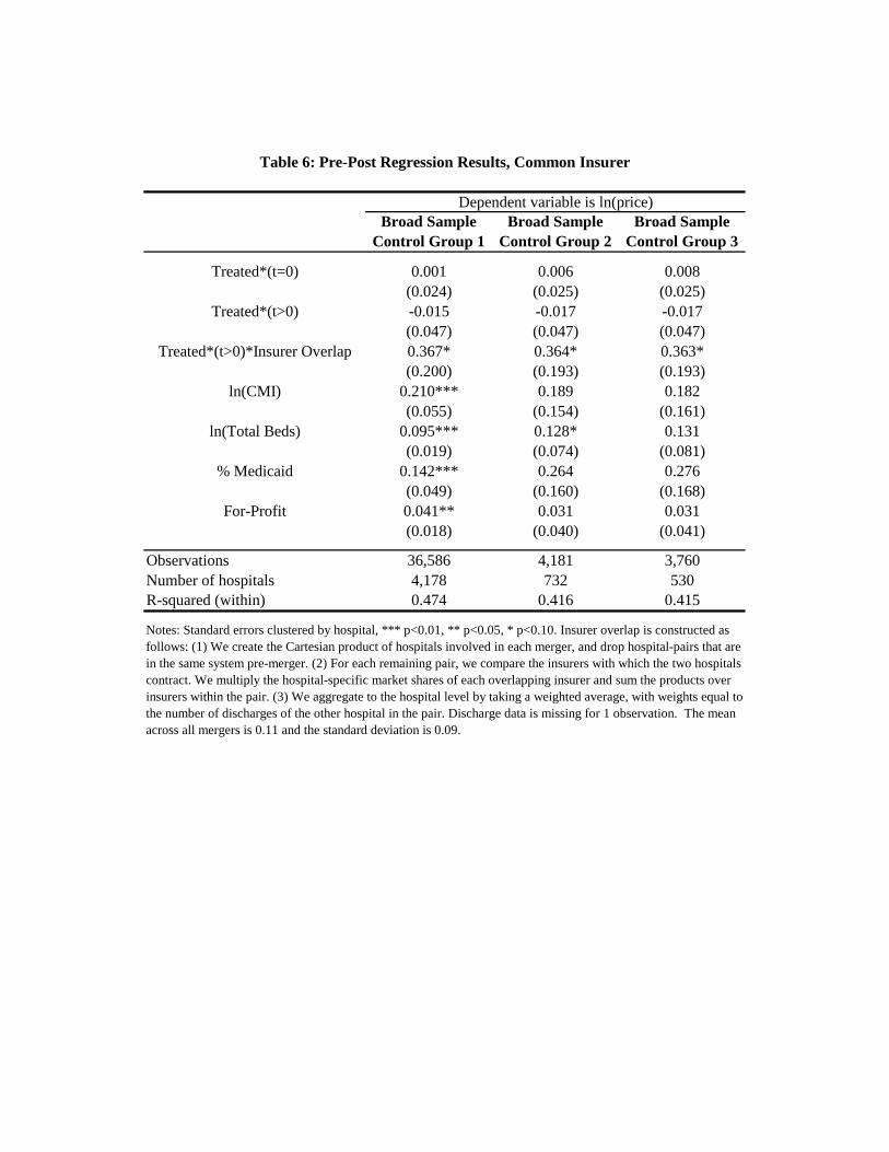
Broad Sample Control Group 1
Broad Sample Control Group 2
Broad Sample Control Group 3
Treated*(t=0) 0.001 0.006 0.008(0.024) (0.025) (0.025)
Treated*(t>0) -0.015 -0.017 -0.017(0.047) (0.047) (0.047)
Treated*(t>0)*Insurer Overlap 0.367* 0.364* 0.363*(0.200) (0.193) (0.193)
ln(CMI) 0.210*** 0.189 0.182(0.055) (0.154) (0.161)
ln(Total Beds) 0.095*** 0.128* 0.131(0.019) (0.074) (0.081)
% Medicaid 0.142*** 0.264 0.276(0.049) (0.160) (0.168)
For-Profit 0.041** 0.031 0.031(0.018) (0.040) (0.041)
Observations 36,586 4,181 3,760Number of hospitals 4,178 732 530R-squared (within) 0.474 0.416 0.415
Dependent variable is ln(price)
Table 6: Pre-Post Regression Results, Common Insurer
Notes: Standard errors clustered by hospital, *** p<0.01, ** p<0.05, * p<0.10. Insurer overlap is constructed as follows: (1) We create the Cartesian product of hospitals involved in each merger, and drop hospital-pairs that are in the same system pre-merger. (2) For each remaining pair, we compare the insurers with which the two hospitals contract. We multiply the hospital-specific market shares of each overlapping insurer and sum the products over insurers within the pair. (3) We aggregate to the hospital level by taking a weighted average, with weights equal to the number of discharges of the other hospital in the pair. Discharge data is missing for 1 observation. The mean across all mergers is 0.11 and the standard deviation is 0.09.


-0.10
-0.05
0.00
0.05
0.10
0.15
0.20
-3 -2 -1 0 1 2 3
Figure 2: FTC Leads & Lags (Control Group 2)
Adjacent Treated Non-Adjacent Treated
-0.10
-0.05
0.00
0.05
0.10
0.15
0.20
-3 -2 -1 0 1 2 3
Figure 3: Broad Sample Leads & Lags (Control Group 3)
Adjacent Treated Non-Adjacent Treated

Adjacent Treated (30-90)
Adjacent Treated (>90)
Non-Adjacent Treated
-3-2 -0.003 0.036 -0.029-1 -0.021 0.031 -0.0390 0.079 -0.025 -0.0751 0.088 0.031 -0.0212 0.100 0.057 -0.0873 0.177 0.139 -0.035
-0.10
-0.05
0.00
0.05
0.10
0.15
0.20
-3 -2 -1 0 1 2 3
Figure 4: Broad Sample Distance Effects (Control Group 3)
Adjacent Treated (30-90) Adjacent Treated (>90) Non-Adjacent Treated

FTC Control Group 1
FTC Control Group 2
Adj Treated*(t=-2) 0.067 0.070*(0.043) (0.042)
Adj Treated*(t=-1) 0.073** 0.072**(0.032) (0.033)
Adj Treated*(t=0) 0.069** 0.066**(0.032) (0.032)
Adj Treated*(t=1) 0.091** 0.091**(0.036) (0.036)
Adj Treated*(t=2) 0.124*** 0.121***(0.033) (0.034)
Adj Treated*(t=3) 0.157*** 0.151***(0.038) (0.038)
Non-Adj Treated*(t=0) -0.040 -0.040(0.057) (0.057)
Non-Adj Treated*(t=1) -0.061 -0.054(0.069) (0.069)
Non-Adj Treated*(t=2) 0.011 0.014(0.063) (0.063)
Non-Adj Treated*(t=3) 0.009 0.010(0.063) (0.062)
ln(CMI) 0.284*** 0.271***(0.048) (0.064)
ln(Total Beds) 0.086*** 0.102***(0.017) (0.022)
% Medicaid 0.095** 0.113**(0.042) (0.058)
For-Profit 0.055*** 0.062***(0.017) (0.020)
Observations 54,347 30,381Number of hospitals 4,816 2,802R-squared (within) 0.552 0.569p-value for H0: coefficients for Adj*(t=3) and Non-Adj*(t=3) are same
0.042 0.052
Appendix Table 1: Leads & Lags Regression Results, FTC Sample
Dependent variable is ln(price)
Notes: Standard errors clustered by hospital, *** p<0.01, ** p<0.05, * p<0.1

Broad Sample Control Group 1
Broad Sample Control Group 2
Broad Sample Control Group 3
Adj Treated*(t=-2) 0.006 0.008 0.009(0.029) (0.030) (0.030)
Adj Treated*(t=-1) 0.004 -0.005 -0.004(0.039) (0.039) (0.039)
Adj Treated*(t=0) 0.039 0.040 0.043(0.037) (0.038) (0.038)
Adj Treated*(t=1) 0.067 0.071 0.069(0.045) (0.045) (0.045)
Adj Treated*(t=2) 0.092 0.082 0.085(0.058) (0.060) (0.060)
Adj Treated*(t=3) 0.170*** 0.166*** 0.165***(0.056) (0.056) (0.056)
Non-Adj Treated*(t=-2) -0.032 -0.031 -0.029(0.047) (0.049) (0.049)
Non-Adj Treated*(t=-1) -0.034 -0.039 -0.039(0.043) (0.044) (0.044)
Non-Adj Treated*(t=0) -0.078 -0.078 -0.076(0.050) (0.052) (0.052)
Non-Adj Treated*(t=1) -0.010 -0.022 -0.022(0.051) (0.053) (0.054)
Non-Adj Treated*(t=2) -0.089 -0.089 -0.087(0.055) (0.058) (0.058)
Non-Adj Treated*(t=3) -0.032 -0.035 -0.034(0.065) (0.069) (0.070)
ln(CMI) 0.210*** 0.188 0.182(0.055) (0.155) (0.161)
ln(Total Beds) 0.094*** 0.127* 0.129(0.019) (0.074) (0.081)
% Medicaid 0.142*** 0.273* 0.285*(0.049) (0.162) (0.170)
For-Profit 0.041** 0.025 0.025(0.018) (0.036) (0.038)
Observations 36,587 4,182 3,761Number of hospitals 4,179 733 531R-squared (within) 0.474 0.418 0.417p-value for H0: coefficients for Adj*(t=3) and Non-Adj*(t=3) are same
0.018 0.019 0.020
Notes: Standard errors clustered by hospital, *** p<0.01, ** p<0.05, * p<0.1
Appendix Table 2: Leads & Lags Regression Results, Broad Sample
Dependent variable is ln(price)

All Tenet / OrNdaInova /
Alexandria
Tenet / Doctors Regional
Sutter / Summit
Piedmont / Newnan
UPMC / Mercy Banner / Sun
St. Elizabeth / St. Luke
Hartford / Central
Connecticut
St. Peters / Northeast /
Seton
Adj Treated*(t=0) 0.009 0.020 0.009 0.008 0.009 0.009 0.006 0.019 0.009 -0.000 0.009(0.017) (0.020) (0.018) (0.018) (0.021) (0.018) (0.018) (0.017) (0.017) (0.016) (0.018)
Adj Treated*(t>0) 0.062** 0.058* 0.063** 0.064** 0.054** 0.064** 0.061** 0.081*** 0.060** 0.055** 0.063**(0.024) (0.033) (0.026) (0.025) (0.025) (0.026) (0.025) (0.024) (0.025) (0.024) (0.025)
Non-Adj Treated*(t=0) -0.039 0.046 -0.039 -0.039 -0.039 -0.039 -0.039 -0.057 -0.039 -0.039 -0.039(0.057) (0.031) (0.057) (0.057) (0.057) (0.057) (0.057) (0.070) (0.057) (0.057) (0.057)
Non-Adj Treated*(t>0) -0.009 0.008 -0.009 -0.009 -0.009 -0.009 -0.009 -0.012 -0.009 -0.009 -0.009(0.055) (0.058) (0.055) (0.055) (0.055) (0.055) (0.055) (0.066) (0.055) (0.055) (0.055)
ln(CMI) 0.271*** 0.271*** 0.271*** 0.270*** 0.272*** 0.270*** 0.271*** 0.271*** 0.270*** 0.271*** 0.271***(0.064) (0.064) (0.064) (0.064) (0.064) (0.064) (0.064) (0.064) (0.064) (0.064) (0.064)
ln(Total Beds) 0.102*** 0.102*** 0.102*** 0.102*** 0.101*** 0.102*** 0.102*** 0.102*** 0.102*** 0.102*** 0.102***(0.022) (0.022) (0.022) (0.022) (0.022) (0.022) (0.022) (0.022) (0.022) (0.022) (0.022)
% Medicaid 0.113** 0.116** 0.113** 0.113** 0.115** 0.113** 0.113** 0.113* 0.113** 0.112* 0.113*(0.058) (0.058) (0.058) (0.058) (0.058) (0.058) (0.058) (0.058) (0.058) (0.058) (0.058)
For-Profit 0.062*** 0.062*** 0.062*** 0.062*** 0.062*** 0.062*** 0.062*** 0.062*** 0.062*** 0.062*** 0.062***(0.020) (0.020) (0.020) (0.020) (0.020) (0.020) (0.020) (0.020) (0.020) (0.020) (0.020)
Observations 30,381 29,988 30,371 30,353 30,265 30,371 30,353 30,323 30,374 30,371 30,371Number of hospitals 2,802 2,717 2,800 2,797 2,784 2,800 2,798 2,792 2,801 2,800 2,800R-squared (within) 0.569 0.570 0.569 0.569 0.569 0.569 0.569 0.569 0.569 0.569 0.569p-value for H0: coefficients for Adj*(t>0) and Non-Adj*(t>0) are same
0.235 0.453 0.235 0.227 0.294 0.227 0.248 0.183 0.250 0.282 0.229
Notes: Standard errors clustered by hospital, *** p<0.01, ** p<0.05, * p<0.1
Excluding:
Appendix Table 3: FTC Pre-Post Regression Results, Dropping One Transaction at a Time (Control Group 2)
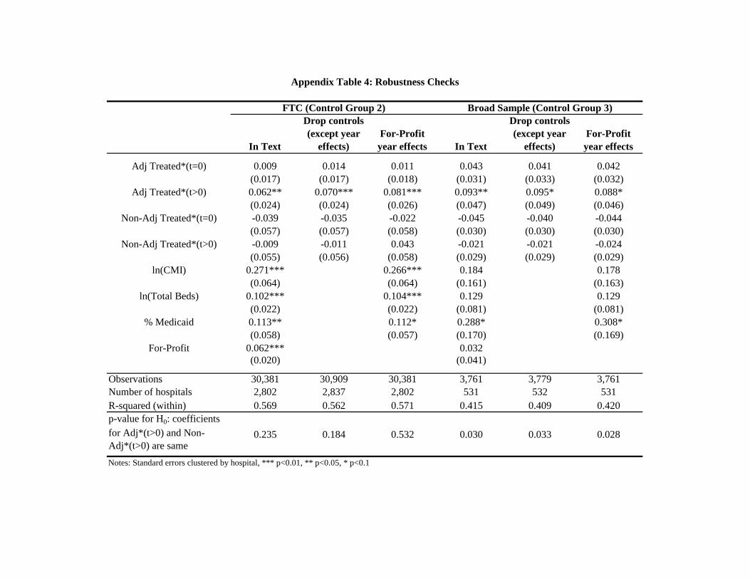
In Text
Drop controls (except year
effects)For-Profit year effects In Text
Drop controls (except year
effects)For-Profit
year effects
Adj Treated*(t=0) 0.009 0.014 0.011 0.043 0.041 0.042(0.017) (0.017) (0.018) (0.031) (0.033) (0.032)
Adj Treated*(t>0) 0.062** 0.070*** 0.081*** 0.093** 0.095* 0.088*(0.024) (0.024) (0.026) (0.047) (0.049) (0.046)
Non-Adj Treated*(t=0) -0.039 -0.035 -0.022 -0.045 -0.040 -0.044(0.057) (0.057) (0.058) (0.030) (0.030) (0.030)
Non-Adj Treated*(t>0) -0.009 -0.011 0.043 -0.021 -0.021 -0.024(0.055) (0.056) (0.058) (0.029) (0.029) (0.029)
ln(CMI) 0.271*** 0.266*** 0.184 0.178(0.064) (0.064) (0.161) (0.163)
ln(Total Beds) 0.102*** 0.104*** 0.129 0.129(0.022) (0.022) (0.081) (0.081)
% Medicaid 0.113** 0.112* 0.288* 0.308*(0.058) (0.057) (0.170) (0.169)
For-Profit 0.062*** 0.032(0.020) (0.041)
Observations 30,381 30,909 30,381 3,761 3,779 3,761Number of hospitals 2,802 2,837 2,802 531 532 531R-squared (within) 0.569 0.562 0.571 0.415 0.409 0.420p-value for H0: coefficients for Adj*(t>0) and Non-Adj*(t>0) are same
0.235 0.184 0.532 0.030 0.033 0.028
Notes: Standard errors clustered by hospital, *** p<0.01, ** p<0.05, * p<0.1
FTC (Control Group 2) Broad Sample (Control Group 3)
Appendix Table 4: Robustness Checks

Broad Sample Control Group 3
Adj Treated*(30-90)*(t=-2) -0.003(0.041)
Adj Treated*(30-90)*(t=-1) -0.021(0.055)
Adj Treated*(30-90)*(t=0) 0.079*(0.047)
Adj Treated*(30-90)*(t=1) 0.088(0.056)
Adj Treated*(30-90)*(t=2) 0.100(0.076)
Adj Treated*(30-90)*(t=3) 0.177**(0.076)
Adj Treated*(>90)*(t=-2) 0.036(0.035)
Adj Treated*(>90)*(t=-1) 0.031(0.044)
Adj Treated*(>90)*(t=0) -0.025(0.051)
Adj Treated*(>90)*(t=1) 0.031(0.070)
Adj Treated*(>90)*(t=2) 0.057(0.086)
Adj Treated*(>90)*(t=3) 0.139***(0.052)
Non-Adj Treated*(t=-2) -0.029(0.049)
Non-Adj Treated*(t=-1) -0.039(0.044)
Non-Adj Treated*(t=0) -0.075(0.052)
Non-Adj Treated*(t=1) -0.021(0.054)
Non-Adj Treated*(t=2) -0.087(0.058)
Non-Adj Treated*(t=3) -0.035(0.070)
ln(CMI) 0.178(0.161)
ln(Total Beds) 0.128(0.081)
% Medicaid 0.281*(0.169)
For-Profit 0.025(0.037)
Observations 3,761Number of hospitals 531R-squared (within) 0.418
Appendix Table 5: Distance Effects
Notes: Standard errors clustered by hospital, *** p<0.01, ** p<0.05, * p<0.1