Embed Size (px)
Citation preview

Available online at www.sciencedirect.com
ScienceDirect
International Journal of Naval Architecture and Ocean Engineering 8 (2016) 153e168http://www.journals.elsevier.com/international-journal-of-naval-architecture-and-ocean-engineering/
The pressure distribution on the rectangular and trapezoidal storage tanks'perimeters due to liquid sloshing phenomenon
Hassan Saghi*
Department of Civil Engineering, Hakim Sabzevar University, Sabzevar, Iran
Received 3 August 2015; revised 6 October 2015; accepted 11 December 2015
Available online 22 February 2016
Abstract
Sloshing phenomenon is a complicated free surface flow problem that increases the dynamic pressure on the sidewalls and the bottom of thestorage tanks. When the storage tanks are partially filled, it is essential to be able to evaluate the fluid dynamic loads on the tank's perimeter. Inthis paper, a numerical code was developed to determine the pressure distribution on the rectangular and trapezoidal storage tanks' perimetersdue to liquid sloshing phenomenon. Assuming the fluid to be inviscid, the Laplace equation and the nonlinear free surface boundary conditionswere solved using coupled boundary element e finite element method. The code performance for sloshing modeling was validated usingNakayama and Washizu's results. Finally, this code was used for partially filled rectangular and trapezoidal storage tanks and free surfacedisplacement, pressure distribution and horizontal and vertical forces exerted on the tanks' perimeters due to liquid sloshing phenomenon wereestimated and discussed.Copyright © 2016 Society of Naval Architects of Korea. Production and hosting by Elsevier B.V. This is an open access article under the CC BY-NC-ND license (http://creativecommons.org/licenses/by-nc-nd/4.0/).
Keywords: Pressure distribution; Liquid sloshing phenomenon; Sway motion; Trapezoidal storage tank; Free surface displacement; Horizontal and vertical forces;
Coupled boundary element-finite element method
1. Introduction
The sloshing phenomenon in a moving container is asso-ciated with various engineering problems, such as tankers onhighways, liquid oscillations in large storage tanks caused byearthquakes, sloshing of liquid cargo in ocean-going vesselsand the motion of liquid fuel in aircraft and spacecraft. Thisphenomenon is of interest in a variety of engineering fields asit may cause large structural loads. Many researchers studiedthis phenomenon in the last few decades. Some researchersconsidered the fluid to be inviscid (Choun and Yun, 1996;Frandsen, 2004; Wu, 2007; Chen et al., 2012; Zhang, 2015a;Zhang et al., 2015; Lee et al., 2007a) while others consid-ered it as viscous (Lee et al., 2007b; Wu et al., 2012; Gomez-
* Tel.: þ98 544012787; fax: þ98 57144410104.
E-mail address: [email protected].
Peer review under responsibility of Society of Naval Architects of Korea.
http://dx.doi.org/10.1016/j.ijnaoe.2015.12.001 / pISSN : 2092-6782, eISSN : 2092
2092-6782/Copyright © 2016 Society of Naval Architects of Korea. Production and
ND license (http://creativecommons.org/licenses/by-nc-nd/4.0/).
Goni et al., 2013; De Chowdhury and Sannasiraj, 2014; JingLi and Zhen Chen, 2014; Zhao and Chen, 2015). Differentgeometric shapes were proposed for storage tanks to model thesloshing phenomenon by researchers. Choun and Yun (1996),Chen and Chiang (2000), Celebi and Akyildiz (2002),Frandsen (2004), Akyildiz and Unal (2006, 2005), Chen andNokes (2005), Wu (2007), Lee et al. (2007a, 2007b), Liuand Lin (2008), Panigrahy et al. (2009), Belakroum et al.(2010), Ming and Duan (2010), Huang et al. (2010), Pirkeret al. (2012) and Lu et al. (2015) studied the sloshing phe-nomenon in rectangular tank. Hasheminejad and Aghabeigi(2012) used an elliptical tank shape. Papaspyrou et al.(2004), Karamanos et al. (2005), Wiesche (2008) andShekari et al. (2009) studied sloshing in cylindrical tanks.Gavrilyuk et al. (2005) studied linear and nonlinear sloshing ina circular conical tank. Mciver (1989), Papaspyrou et al.(2003), Patkas and Karamanos (2007), Yue (2008) andCuradelli et al. (2010) modeled sloshing in spherical tanks.Some researchers such as Liu and Lin (2009), Panigrahy et al.
-6790
hosting by Elsevier B.V. This is an open access article under the CC BY-NC-
154 H. Saghi / International Journal of Naval Architecture and Ocean Engineering 8 (2016) 153e168
(2009) and Jung et al. (2012) used horizontal and verticalbaffles inside the tank to prevent sloshing with different geo-metric shapes. Ketabdari et al. (2015), Ketabdari and Saghi(2013a, 2013b, 2013c), Saghi and Ketabdari (2012) andZhang (2015b) studied the behavior of the trapezoidal storagetank with linear and nonlinear sidewalls due to liquid sloshingphenomenon. Zou et al. (2015) studied the effects of boundarylayer grid, liquid viscosity and compressible air on sloshingpressure, wave height and rising time of impact pressure. Leeet al. (2013) evaluated the sloshing resistance performance ofa huge-size LNG carrier's insulation system by the fluid-estructure interaction (FSI) analysis. Jung et al. (2015) stud-ied the effect of natural frequency modes on sloshingphenomenon in a rectangular tank. Kim (2013) calculated therapid response of LNG cargo containment system undersloshing load using wavelet transformation method.
The principal objective of this study is to develop a nu-merical model assuming incompressible and inviscid fluid inthe rectangular and trapezoidal storage tanks to find the freesurface displacement, pressure distribution, horizontal andvertical forces exerted on the tank's perimeter that is causeddue to liquid sloshing phenomenon. The coupled boundaryelement e finite element methods were used to solve theLaplace equation and the nonlinear free surface boundaryconditions to model the sloshing phenomenon.
2. Problem definition
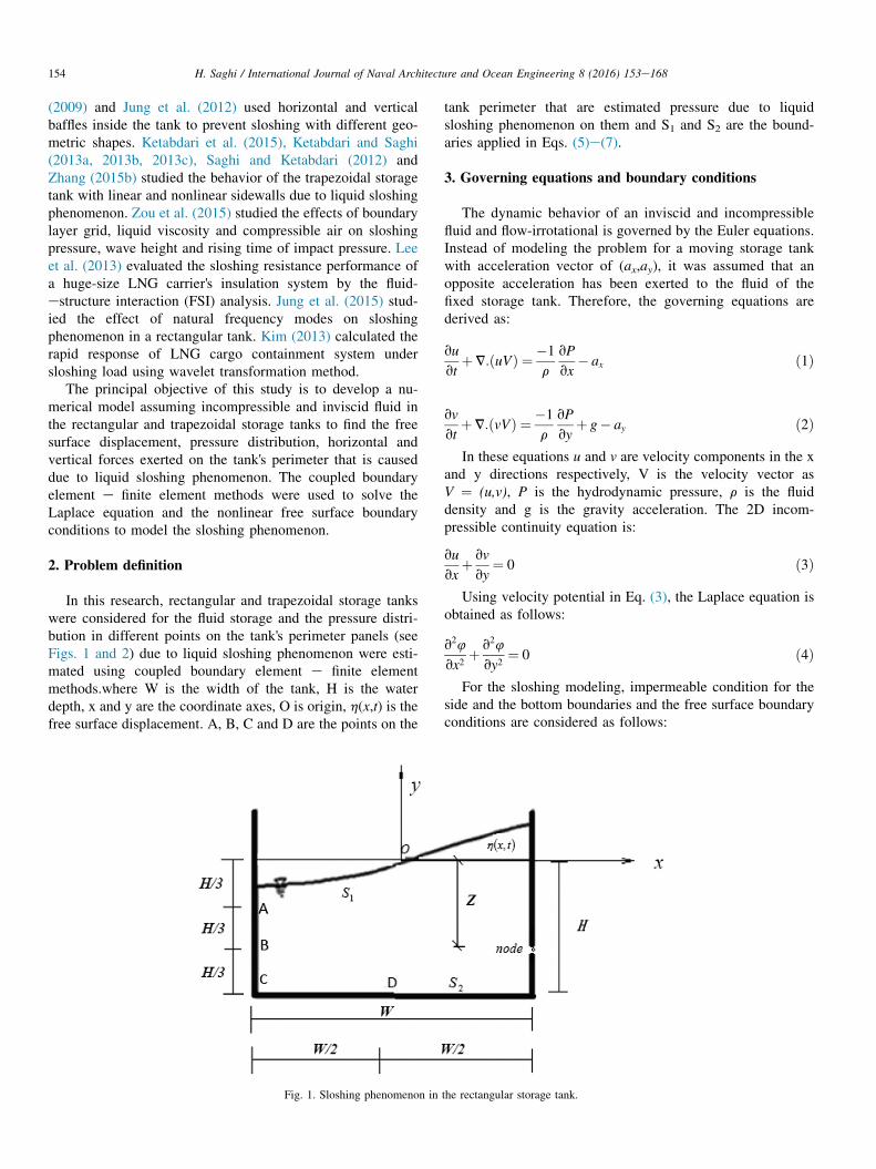
In this research, rectangular and trapezoidal storage tankswere considered for the fluid storage and the pressure distri-bution in different points on the tank's perimeter panels (seeFigs. 1 and 2) due to liquid sloshing phenomenon were esti-mated using coupled boundary element e finite elementmethods.where W is the width of the tank, H is the waterdepth, x and y are the coordinate axes, O is origin, h(x,t) is thefree surface displacement. A, B, C and D are the points on the
Fig. 1. Sloshing phenomenon in
tank perimeter that are estimated pressure due to liquidsloshing phenomenon on them and S1 and S2 are the bound-aries applied in Eqs. (5)e(7).
3. Governing equations and boundary conditions
The dynamic behavior of an inviscid and incompressiblefluid and flow-irrotational is governed by the Euler equations.Instead of modeling the problem for a moving storage tankwith acceleration vector of (ax,ay), it was assumed that anopposite acceleration has been exerted to the fluid of thefixed storage tank. Therefore, the governing equations arederived as:
vu
vtþV:ðuVÞ ¼ �1
r
vP
vx� ax ð1Þ
vv
vtþV:ðvVÞ ¼ �1
r
vP
vyþ g� ay ð2Þ
In these equations u and v are velocity components in the xand y directions respectively, V is the velocity vector asV ¼ (u,v), P is the hydrodynamic pressure, r is the fluiddensity and g is the gravity acceleration. The 2D incom-pressible continuity equation is:
vu
vxþ vv
vy¼ 0 ð3Þ
Using velocity potential in Eq. (3), the Laplace equation isobtained as follows:
v24
vx2þ v24
vy2¼ 0 ð4Þ
For the sloshing modeling, impermeable condition for theside and the bottom boundaries and the free surface boundaryconditions are considered as follows:
the rectangular storage tank.

Fig. 3. Description of calculation domain of boundary integral.
Fig. 2. Sloshing phenomenon in the trapezoidal storage tank.
155H. Saghi / International Journal of Naval Architecture and Ocean Engineering 8 (2016) 153e168
v4
vn¼ 0 on S2: ð5Þ
v4
vn¼ ny
vh
vton S1 ð6Þ
v4
vtþ 1
2
�v4
vx
�2
þ�v4
vy
�2!þ �ay þ g
�hbþ axx¼ 0 on S1
ð7Þwhere ny is the y-component of the normal unit vector to theelement surface, h is the free surface displacement, b is uniquefor rectangular and sinq (see Fig. 2) for trapezoidal storagetanks, S1 and S2 are illustrated in Figs. 1 and 2 and 4 is ve-locity potential. In order to model the sloshing phenomenon,the Laplace equation and the dynamic free surface boundarycondition are solved simultaneously using coupled boundaryelement e finite element methods. The results of the model arefree surface displacement (h) and potential function (4) thatare used for estimation of pressure distribution and horizontaland vertical forces exerted on the tank perimeter.
4. Mathematical modeling
In order to model the sloshing phenomenon in the tank, theLaplace equation and the dynamic free surface boundarycondition (Eqs. (4) and (7)) were solved simultaneously usingcoupled boundary element-finite element methods.
4.1. Laplace equation
Fig. 4. Description of a(x) in x node of boundary.
The Laplace equation was solved using boundary elementmethod and the Green's theorem as follows:
cðxÞ4ðxÞþIvD
4ðyÞvjvn
ðx;yÞdsðyÞ
¼ZvD
jðx;yÞv4vn
ðyÞdsðyÞ x; y2vD
ð8Þ
In this equation j(x,y) is the fundamental solution, equal to12p ln
1r for 2D problems, where r is the space between the nodes
which is calculated from node x based on other perimeter nodes(y). Fig. 3 shows the calculation domain of the boundary Integral.
In this Figure, D is the domain integrals, z is the internalnode, y is the perimeter nodes, x is the nodal boundary, vDk isthe boundary integral and vD
εis the boundary integral adja-
cent to node x. c(x) is a constant calculated based on the ge-ometry of the boundary in node x as:
cðxÞ ¼ aðxÞ2p
ð9Þ
where a(x) is the angle between two tangent lines to x nodalboundary as shown in Fig. 4.
In this step, domain integrals (D) are replaced by boundaryintegrals (vD) in Eq.(8) using Green theorem. SubstitutingEqs. (5) and (6) into Eq.(8) leads to (S ¼ S1 þ S2):
cðlÞ4ðlÞ þZs
4v
vn
�1
2pln1
r
�ds¼
Zs1
nyvh
vt
�1
2pln1
r
�ds ð10Þ
4kðzÞ ¼ ½N1ðzÞ N2ðzÞ��
4kðkÞ4kðkþ 1Þ
�ð11Þ

156 H. Saghi / International Journal of Naval Architecture and Ocean Engineering 8 (2016) 153e168
hkðzÞ ¼ ½N1ðzÞ N2ðzÞ��
hkðkÞhkðkþ 1Þ
�ð12Þ
N1(z) and N2(z) are the linear shape functions as follows:
N1ðzÞ ¼ 1� z ð13Þ
N2ðzÞ ¼ z ð14Þ
cðlÞD4l þXKk¼1
½A1ðl;kÞ A2ðl; kÞ �"
D4k
D4kþ1
#�XK0
k¼1
½B1ðl;kÞ B2ðl;kÞ �:
26666664
2
Dtn0ykDhk þ
n0yk�h0k � h0
kþ1
�l20k
�vh
vt
�0k
Dhk þn0yk�h0kþ1 � h0
k
�l20k
�vh
vt
�0k
Dhkþ1
2
Dtn0ykDhkþ1 þ
n0yk�h0k � h0
kþ1
�l20k
�vh
vt
�0kþ1
Dhk þn0yk�h0kþ1 � h0
k
�l20k
�vh
vt
�0kþ1
Dhkþ1
37777775
¼�cðlÞ40l�XKk¼1
½A1ðl;kÞ A2ðl;kÞ �"
40k
40kþ1
#�XK 0
k¼1
½B1ðl;kÞ B2ðl;kÞ �
2666664
n0yk
�vh
vt
�0k
n0yk
�vh
vt
�0kþ1
3777775
ð22Þ
where z is the local coordinate of element. Substituting Eqs.(11)e(14) into Eq. (10) leads to:
cðlÞ4ðlÞþXKk¼1
ZvDk
½N1ðzÞ N2ðzÞ��
4kðkÞ4kðkþ1Þ
�1
2p
v
vn
�ln1
r
�Lk
2dz
¼XK0
k¼1
ZvDk0
ny½N1ðzÞ N2ðzÞ��
_hkðkÞ_hkðkþ1Þ
�1
2pln1
r
Lk
2dz
ð15ÞvDk, vDk
0, k and k0 are the boundary elements and element
numbers in the domain and free surface respectively. The re-lationships between some parameters for the new and old timelevels can be expressed as:
4¼ 40 þD4 ð16Þ
h¼ h0 þDh ð17Þ
v4
vt¼ 2
DtD4�
�v4
vt
�0
ð18Þ
vh
vt¼ 2
DtDh�
�vh
vt
�0
ð19Þ
l¼ l0 þ�h0j � h0
jþ1
�Dhj �Dhjþ1
�l0
ð20Þ
ny ¼ n0y �n0yl20
�h0j � h0
jþ1
:�Dhj �Dhjþ1
� ð21Þ
where l is the surface element length and 0 refers to theprevious time level. Substituting Eqs. (16)e(21) in Eq. (15)leads to:
Aaðl;kÞ ¼Z
NaðzÞqjðl;zÞ l dz a¼ 1; 2 ð23Þ
vDk2
Baðl;kÞ ¼ZvDk
NaðzÞjðl;zÞ l2dz a¼ 1; 2 ð24Þ
qðyÞ ¼ v4
vnðyÞ ð25Þ
qjðl;yÞ ¼ vj
vnðl;yÞ ð26Þ
4.2. Dynamic free surface boundary condition
In this research, finite element method was used for thedynamic free surface boundary condition solution. Errorcorrection term denoted by D was applied to solve thisequation as:
vD
vt¼ v4
vtþ 1
2
(�v4
vx
�2
þ�v4
vy
�2)þ axxþ
�gþ ay
�hb ð27Þ
Considering Eqs. (7) and (27) is merely valid when D iszero at any time step. Using Galerkin method to solve thisequation, residual (Re) of a general function such as f(s,t) canbe estimated as:

157H. Saghi / International Journal of Naval Architecture and Ocean Engineering 8 (2016) 153e168
Re¼Z l
s¼0
Nf ðs; tÞds ð28Þ
where N ¼ [N1(z)N2(z)]. Now considering Eq. (27) as f(s,t)and combining Eqs. (13), (14) and (28) leads to:
Re j¼Z l
s¼0
1
l
�l� s
s
� v4
vtþ1
2
"n2y
�vh
vt
�2
þ�v4
vs
�2#þaxx
þ�ayþg�h� _D
!ds
ð29Þ
The parameter z in these equations was replaced bys/l.Using Eq. (29) and v4/vs ¼ (4j þ 1 � 4j)/lj, residuals of node j
lj
�1
3_4j þ
1
6_4jþ1
�þ 1
24ljn
2yj
�3 _h2
j þ 2 _hjþ1 _hj þ _h2jþ1
þ 1
4lj
�4j �4jþ1
�2þ lj
ax
�1
3xj þ 1
6xjþ1
�þ �gþ ay
��13hj þ
1
6hjþ1
���1
3_Dj þ 1
6_Djþ1
��
þ lj�1
�1
6_4j�1 þ
1
3_4j
�þ 1
24lj�1n
2yj�1
�_h2j�1 þ 2 _hj _hj�1 þ 3 _h2
j
þ 1
4lj�1
�4j�1 �4j
�2þ lj�1
ax
�1
6xj�1 þ 1
3xj
�þ �gþ ay
��16hj�1 þ
1
3hj
���1
6_Dj�1 þ 1
3_Dj
��¼ 0
ð33Þ
in two adjacent elements (j and j-1) were obtained as:
Re jj ¼lj
�1
3_4j þ
1
6_4jþ1
�þ 1
24ljn
2yj
�3 _h2
j þ 2 _hjþ1 _hj þ _h2jþ1
þ 1
4lj
�4j �4jþ1
�2 þ lj
ax
�1
3xj þ 1
6xjþ1
�
þ �gþ ay��1
3hj þ
1
6hjþ1
���1
3_Dj þ 1
6_Djþ1
��¼ 0
ð30Þ
Aj ¼� h0
j � h0jþ1
3l0j
�v4
vt
�0j
� h0j � h0
jþ1
6l0j
�v4
vt
�0jþ1
þ 1
24n0
2
yjl0j
"�12
Dt
�"3
�vh
vt
�2
0j
þ 2
�vh
vt
�0jþ1
�vh
vt
�0j
þ�vh
vt
�2
0jþ1
#þ ax
h0j � h0
jþ1
l0j
�1
3
� h0j � h0
jþ1
l0j
�1
3_Dj þ 1
6_Djþ1
�þ h0
j � h0j�1
l0j�1
"� 1
6
�v4
vt
�0j�1
� 1
3
�
�n0
2
yj�1
�h0j � h0
j�1
24l0j�1
"�vh
vt
�2
0j�1
þ 2
�vh
vt
�0j
�vh
vt
�0j�1
þ 3
�vh
vt
�2
0
þ �ay þ g��1
6h0j�1 þ
1
3h0j
���1
6_Dj�1 þ 1
3_Dj
���
Re j�1j ¼lj�1
�1
6_4j�1 þ
1
3_4j
�þ 1
24lj�1n
2yj�1
�_h2j�1 þ 2 _hj _hj�1
þ 3 _h2j
þ 1
4lj�1
�4j�1 �4j
�2 þ lj�1
ax
�1
6xj�1 þ 1
3xj
�
þ �gþ ay��1
6hj�1 þ
1
3hj
���1
6_Dj�1 þ 1
3_Dj
��¼ 0
ð31Þwhere a and b in the Reba are the node and element numbers,respectively. Total residual of node j in two adjacent elementsmust be zero. Thus:
Rejj þRej�1j ¼ 0 ð32Þ
Substituting Eqs. (30) and (31) into Eq. (32) leads to:
Substituting Eqs. (16)e(21) into Eq. (33) leads to:
AjDhj þAjþ1Dhjþ1 þAj�1Dhj�1 þBj�1D4j�1 þBjD4j
þBjþ1D4jþ1¼ C ð34Þ
where
vh
vt
�0j
� 4
Dt
�vh
vt
�0jþ1
#�n0
2
yj
�h0j � h0
jþ1
24l0j
xj þ 1
6xjþ1
�þ l0j
�ay þ g
�3
þ h0j � h0
jþ1
l0j
�ay þ g
��13h0j þ
1
6h0jþ1
�
v4
vt
�0j
#þ 1
24l0j�1
n02
yj�1
"�4
Dt
�vh
vt
�0j�1
� 12
Dt
�vh
vt
�0j
#
j
#þ l0j�1
�ay þ g
�3
þ h0j � h0
j�1
l0j�1
�ax
�1
6xj�1 þ 1
3xj
�
ð35Þ

Fig. 5. Schematic diagram of Rectangular tank node arrangement.
158 H. Saghi / International Journal of Naval Architecture and Ocean Engineering 8 (2016) 153e168
Ajþ1 ¼� h0
jþ1 � h0j
3l0j
�v4
vt
�0j
� h0jþ1 � h0
j
6l0j
�v4
vt
�0jþ1
þ 1
24n0
2
yjl0j
"�4
Dt
�vh
vt
�0j
� 4
Dt
�vh
vt
�0jþ1
#
�n0
2
yj
�h0jþ1 � h0
j
24l0j
"3
�vh
vt
�2
0j
þ 2
�vh
vt
�0jþ1
�vh
vt
�0j
þ�vh
vt
�2
0jþ1
#þ l0j
�ay þ g
�6
þ h0jþ1 � h0
j
l0jax
��1
3xj þ 1
6xjþ1
�þ h0
jþ1 � h0j
l0j
�gþ ay
��13h0j þ
1
6h0jþ1
�
� h0jþ1 � h0
j
l0j
�1
3_Dj þ 1
6_Djþ1
��ð36Þ
Aj�1 ¼(n0j�1 � h0
j
"� 1
6
�v4
vt
�0j�1
� 1
3
�v4
vt
�0j
#þ 1
24l0j�1
n02
yj�1
�"�4
Dt
�vh
vt
�0j�1
� 4
Dt
�vh
vt 0j
�#þn0
2
yj�1
�h0j � h0
j�1
24l0j�1
�"�
vh
vt
�2
0j�1
þ 2
�vh
vt
�0j
�vh
vt
�0j�1
þ 3
�vh
vt
�2
0j
#
þ l0j�1
�ay þ g
�6
þ h0j�1 � h0
j
l0j�1
�ax
�1
6xj�1 þ 1
3xj
�
þ �ay þ g��1
6h0j�1 þ
1
3h0j
���1
6_Dj�1 þ 1
3_Dj
���ð37Þ
Bj�1 ¼�
1
3Dtl0j�1
þ 240j�1� 240j
4l0j�1
�ð38Þ
Bj ¼�
2
3Dtl0j þ
240j � 240jþ1
4l0jþ 2
3Dtl0j�1
þ 240j � 240j�1
4l0j�1
�ð39Þ
Bjþ1 ¼�
1
3Dtl0j þ
240jþ1� 240j
4l0j
�ð40Þ
C ¼ C1 þC2 ð41Þ
C1 ¼ 1
3l0j
�v4
vt
�0j
þ 1
6l0j
�v4
vt
�0jþ1
�n0
2
yjl0j
24
"3
�vh
vt
�2
0j
þ 2
�vh
vt
�0jþ1
�vh
vt
�0j
þ�vh
vt
�2
0jþ1
#��40j �40jþ1
2ð42Þ
C2 ¼�ax
�1
3xj þ 1
6xjþ1
�l0j � l0j
�ay þ g
��13h0j þ
1
6h0jþ1
�
þ l0j
�1
3_Dj þ 1
6_Djþ1
�þ"1
6
�v4
vt
�0j�1
þ 1
3
�v4
vt
�0j
#l0j�1
�n0
2
yj�1l0j�1
24x½�vh
vt
�2
0j�1
þ 2
�vh
vt
�0j
�vh
vt
�0j�1
þ 3
�vh
vt
�2
0j
#
��40j �40j�1
2� l0j�1
ax
�1
6xj�1 þ 1
3xj
�
� �gþ ay�l0j�1
�1
6h0j�1 þ
1
3h0j
�þ l0j�1
�1
6_Dj�1 þ 1
3_Dj
�ð43Þ
Finally, Eqs. (22) and (34) were solved simultaneously toestimate D4 and Dh. New velocity potential and free surfaceprofile were estimated using Eqs. (16) and (17) respectively. Inthese equations, parameter D which is unknown can becalculated using Eq. (33). This equation was rearranged as:
lj�1
6_Dj�1 þ
�lj3þ lj�1
3
�_Dj þ lj
6_Djþ1 ¼ lj
�1
3_4j þ
1
6_4jþ1
�
þ 1
24ljn
2yj
�3 _h2
j þ 2 _hjþ1 _hj þ _h2jþ1
þ 1
4lj
�4j �4jþ1
�2þ lj
ax
�1
3xj þ 1
6xjþ1
�þ �gþ ay
��13hj þ
1
6hjþ1
��
þ lj�1
�1
6_4j�1 þ
1
3_4j
�þ 1
24lj�1n
2yj�1
�_h2j�1 þ 2 _hj _hj�1 þ 3 _h2
j
þ 1
4lj�1
�4j�1 �4j
�2 þ lj�1
ax
�1
6xj�1 þ 1
3xj
�þ �gþ ay
���1
6hj�1 þ
1
3hj
��ð44Þ
This equation was solved using Three Diagonal MatrixAlgorithm (TDMA) method and the parameters _Dj�1, _Dj and_Djþ1 were obtained. Finally, parameter D in the new time levelðDt0þDtÞ for all nodes were estimated based on old time levelones ðDt0Þ using finite difference method as:

Fig. 6. Schematic diagram of Trapezoidal tank node arrangement.
Table 1
Effective parameters and their relative nodes in the tank sloshing phenomenon.
Parameter From node To node
Potential function (4) n ntFree surface displacement (h) ns þ 1 ntperimeter pressure (p) n1 ns
Fig. 7. Nodal displacement time histories on the free surface in c
Fig. 8. Nodal displacement time histories on the free surface in
159H. Saghi / International Journal of Naval Architecture and Ocean Engineering 8 (2016) 153e168
Dt0þDtjj ¼ Dt0 jj þDt _Dj ð45ÞHydrodynamic pressure ( pH) and total (Hydrodynamic and
hydro static) Pressure ( pT) distributions on the tank perimeterwere estimated as follows:
pH ¼�rvf
vt� 1
2rðVfÞ2 ð46Þ
pT ¼�rvf
vt� 1
2rðVfÞ2 þ rgZ ð47Þ
where r is the fluid density and Z is distance between nodeestimated pressure on it and the Origin (See Figs. 1 and 2).Total horizontal and vertical forces exerted on the tankperimeter were estimated using Eqs. (48) and (49)respectively:
Fx ¼Xnsi¼1
1
2
�pTI þ pTiþ1
�Li;iþ1nxi;iþ1
ð48Þ
Fy ¼Xnsi¼1
1
2
�pTi þ pTiþ1
�Li;iþ1nyi;iþ1
ð49Þ
Fx and Fx are the total horizontal and vertical forcesexerted on the tank perimeter respectively, ns in the numberof nodes on the storage tank (solid) boundary, pTi and pTiþ1
are the total pressure on the nodes i and iþ1 respectively,
ontact with the right hand sidewall for different mesh sizes.
contact with the right hand sidewall for different time steps.

Fig. 9. Comparison of model surface node displacements and Nakayama and Washizu results (Zou et al., 2015).
Fig. 10. Explanation of max free surface displacement.
Fig. 11. Max free surface displacement for rectangular tanks with 0.6 m water depth and different tank widths (W).
160 H. Saghi / International Journal of Naval Architecture and Ocean Engineering 8 (2016) 153e168
Li,i þ 1 is the length of element between nodes i and i þ 1and nxi;iþ1
and nyi;iþ1are the components of unit vector
perpendicular to the element along the x and y directionsrespectively.
To model the sloshing phenomenon, the potential function(4), the free surface displacement (h) and the perimeterpressure (p) were estimated in the nodes as shown in Figs. 5and 6 and listed in Table 1.

Fig. 12. Max free surface displacement for rectangular tanks with different water depth.
161H. Saghi / International Journal of Naval Architecture and Ocean Engineering 8 (2016) 153e168
5. Model validation
In order to validate the model, a rectangular tank with 0.9 mwidth and 0.6 m water depth was exposed to a horizontal peri-odic sway motion as X ¼ 0.002sin(5.5t). Therefore,ax ¼ �0.0605sin(5.5t) was considered to be the exciting ac-celeration. The displacement of a node on the free surface incontact with the right hand sidewall was calculated by themodel. At the first step, mesh size independently was evaluated.Therefore,Dt¼ 0.0025 s and different mesh sizes l in a range of0.04e0.07 m were used and the results presented in Fig. 7.
It can be seen that an acceptable consistency exists betweenthe results. Moreover, a mesh independently is evident forl � 0.05 m. Therefore l ¼ 0.05 m was used for futurecalculations.
Fig. 13. Area of the tank for rectangular tanks with
In this step, different time steps (Dt) in the range of0.002e0.004 s were used and the results presented in Fig. 8.
It can be seen that an acceptable consistency exists betweenthe results. Furthermore, a time step independently is evidentfor Dt � 0.0025 s. Thus Dt ¼ 0.0025 s was used for futurecalculations. Finally, the results of the numerical model werecompared with those of Nakayama et al. (1984) as shown inFig. 9. It can be seen in this figure that the agreement betweenthe results is well established.
6. Numerical results
In this research, sloshing phenomenon was modeled in therectangular and trapezoidal storage tanks with different width,water depth and sidewall angles. Some parameters such as free
different aspect ratio (width to water depth).

Fig. 14. Nodal displacement time histories on the free surface in contact with the right hand sidewall for different time steps in rectangular and trapezoidal tanks
with a width of 0.9 m, water depth of 0.6 m.
Table 2
Maximum displacement of the free surface in
trapezoidal and rectangular tanks with a width of
0.9 m, water depth of 0.6 m.
Side wall angle Dh(cm)
80 1.92
90 10.34
100 5.61
110 2.7
162 H. Saghi / International Journal of Naval Architecture and Ocean Engineering 8 (2016) 153e168
surface displacement, pressure distribution, horizontal andvertical forces exerted on the tank perimeter were estimatedand discussed.
6.1. Free surface displacement
6.1.1. Free surface displacement on the rectangular storagetanks
In this step, rectangular tanks with 0.6 m water depth anddifferent widths (W) were exposed to a horizontal periodic
Fig. 15. Hydrodynamic pressure distribution on the tank perimeter of rectangular tan
periodic sway motion as X ¼ 0.002sin(5.5t).
sway motion as X ¼ 0.002sin(5.5t) and maximum free surfacedisplacement (hmax) (as explained in Fig. 10) were estimatedand shown in Fig. 11.
The results show that the maximum free surface displace-ment has a relation with the width of the tank as follows:
hmax ¼ 296:67w3 � 603:5w2 þ 412:08w� 93:43 ð50ÞIn the next step, rectangular tanks with 0.9 m width and
different water depths were exposed to a horizontal periodicsway motion as X ¼ 0.002sin(5.5t) and the maximum freesurface displacement was estimated and shown in Fig. 12.
The results show that water depth increasing in the rect-angular tank with constant width has a low effect on themaximum free surface displacement. However, the minimumwater level fluctuation takes place at 0.83 m water depth.
In the next step, rectangular tanks with constant volume(0.54 m3) and different widths and water depths were exposedto a horizontal periodic sway motion as X ¼ 0.002sin(5.5t) andthe maximum free surface displacement was estimated. Then,area of the tank was calculated using Eq. (51) and shown inFig. 13:
k with a width of 0.9 m and a water depth of 0.6 m was exposed to a horizontal

Fig. 16. Total pressure distribution on the tank perimeter of rectangular tank with a width of 0.9 m and a water depth of 0.6 m was exposed to a horizontal periodic
sway motion as X ¼ 0.002sin(5.5t).
Table 3
Maximum and minimum hydrodynamic pressure in the different points of
rectangular tank with a width of 0.9 m and a water depth of 0.6 m was exposed
to a horizontal periodic sway motion as X ¼ 0.002sin(5.5t).
Point Z (m) Pmax (kg/m2) Pmin (kg/m
2) DP (kg/m2)
A 0.2 153.496 �207.405 360.9007
B 0.4 83.0326 �140.393 223.4251
C 0.6 76.5299 �127.337 203.8672
D 0.6 51.0439 �36.8945 87.9384
163H. Saghi / International Journal of Naval Architecture and Ocean Engineering 8 (2016) 153e168
At ¼ 2ðH þ hmaxÞW ð51Þ
The results show that area of the tank (At) is minimizedwhen the aspect ratio (tank width to water depth) be about 0.9.
6.1.2. Free surface displacement on the trapezoidal storagetank
In this section, trapezoidal storage tanks with 0.9 m width,0.6 m water depth and different sidewall angles (see Fig. 2)were exposed to a horizontal periodic sway motion asX ¼ 0.002sin(5.5t). Nodal displacement time histories on thefree surface in contact with the right hand sidewall wereestimated for different time steps and shown in Fig. 14.
In this step, the maximum free surface fluctuation (Dh) wasestimated for the trapezoidal storage tanks with differentsidewalls based on the results shown in Fig. 14 and
summarized in Table 2. The results show that the free surfacefluctuation in the trapezoidal storage tanks arrive to themaximum value in less time in comparison with the rectan-gular storage tank.
The results show that the free surface fluctuation in thetrapezoidal storage tanks arrive to the maximum value in lesstime in comparison with the rectangular storage tank.Furthermore, the maximum free surface fluctuation (Dh) in thetrapezoidal tanks is considerably reduced in comparison withthe rectangular one.
6.2. Pressure distribution on the tank perimeter
6.2.1. Pressure distribution on the rectangular storage tankIn this section, a rectangular tank with 0.9 m width and
0.6 m water depth was exposed to a horizontal periodic swaymotion as X ¼ 0.002sin(5.5t). Hydrodynamic and total pres-sure distributions on the tank perimeter were estimated usingEqs. (46) and (47) and shown in Figs. 15 and 16 respectively.
In this step, the maximum and minimum hydrodynamicpressures on different points (see Fig. 1) were estimated andsummarized in Table 3.
The results show that the total pressure on the tankperimeter increase from points A to D and the hydrodynamicpressure fluctuation decrease from points A to D.

Fig. 17. Total pressure on the different points of trapezoidal storage tank with a width of 0.9 m, water depth of 0.6 m and different sidewall angle, were exposed to a
horizontal periodic sway motion as X ¼ 0.002sin(5.5t).
Table 4
Maximum pressure fluctuation (Dp) for trapezoidal tanks with different side
wall angles.
Point q ¼ 80� q ¼ 90� q ¼ 100� q ¼ 110�
A 52.1832 96.2473 36.7588 44.918
B 24.5988 156.144 60.5096 47.9518
C 32.3923 288.372 144.721 88.127
D 16.7848 87.9383 33.0468 14.2007
Fig. 18. Horizontal force exerted on the tank perimeter of rectangular tank with a w
sway motion as X ¼ 0.002sin(5.5t).
164 H. Saghi / International Journal of Naval Architecture and Ocean Engineering 8 (2016) 153e168
6.2.2. Pressure distribution on the trapezoidal storage tankIn this step, trapezoidal storage tanks with 0.9 m width,
0.6 m water depth and different sidewall angles were exposedto a horizontal periodic sway motion as X ¼ 0.002sin(5.5t) andthe total pressure on the points A, B, C and D were estimatedand shown in Fig. 17.
The maximum pressure fluctuations for the trapezoidaltanks with the different sidewall angles were derived from theresults shown in Fig. 17 and summarized in Table 4. The re-sults show that the maximum pressure fluctuation on thetrapezoidal tank perimeter is less than the rectangular one.
idth of 0.9 m and different water depths was exposed to a horizontal periodic
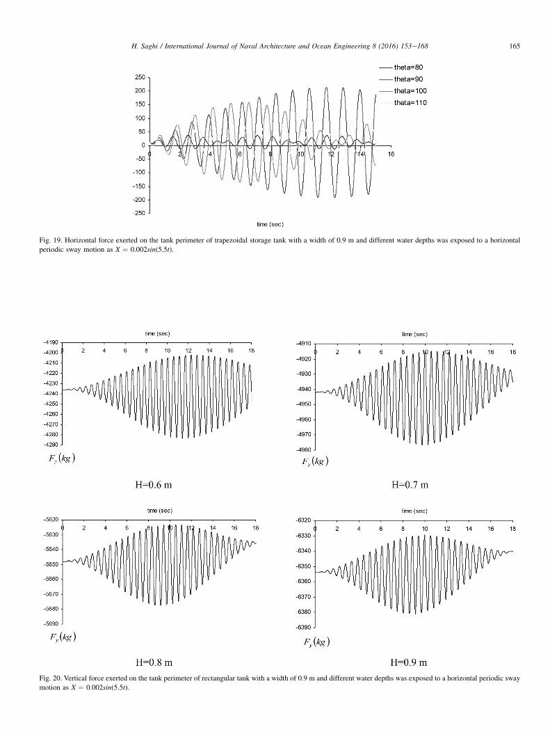
Fig. 19. Horizontal force exerted on the tank perimeter of trapezoidal storage tank with a width of 0.9 m and different water depths was exposed to a horizontal
periodic sway motion as X ¼ 0.002sin(5.5t).
Fig. 20. Vertical force exerted on the tank perimeter of rectangular tank with a width of 0.9 m and different water depths was exposed to a horizontal periodic sway
motion as X ¼ 0.002sin(5.5t).
165H. Saghi / International Journal of Naval Architecture and Ocean Engineering 8 (2016) 153e168

Fig. 21. Vertical force exerted on the tank perimeter of trapezoidal storage tank with a width of 0.9 m and different water depths was exposed to a horizontal
periodic sway motion as X ¼ 0.002sin(5.5t).
166 H. Saghi / International Journal of Naval Architecture and Ocean Engineering 8 (2016) 153e168
6.3. The exertion of the horizontal force on the tankperimeter
6.3.1. The exertion of the horizontal force on the tankperimeter of the rectangular storage tank
In this section, a rectangular tank with 0.9 m width anddifferent water depths were exposed to a horizontal periodicsway motion as X ¼ 0.002sin(5.5t) and the horizontal forceexerted on the tank perimeter was estimated using Eq. (48) andshown in Fig. 18.
The results show that pressure fluctuation for differentwater depths is the same at the beginning. But it is increasedwhen the water depth is decreased.
6.3.2. The exertion of the horizontal force on the tankperimeter of the trapezoidal storage tank
In this section, trapezoidal tanks with 0.9 m width, 0.6 mwater depth and different sidewalls were exposed to a hori-zontal periodic sway motion as X ¼ 0.002sin(5.5t) and thehorizontal force exerted on the tank perimeter were estimatedusing Eq. (48) and shown in Fig. 19. The results show that the
horizontal force exerted on the tank perimeter in the trape-zoidal tanks is considerably reduced in comparison with therectangular one.
6.4. The exertion of the vertical force on the tankperimeter
6.4.1. The exertion of the vertical force on the tankperimeter of the rectangular storage tank
In this section, a rectangular tank with 0.9 m width anddifferent water depths were exposed to a horizontal periodicsway motion as X ¼ 0.002sin(5.5t) and the vertical forceexerted on the tank perimeter was estimated using Eq. (48) andshown in Fig. 20. The results show that the vertical forcefluctuation on the tank perimeter is decreased at the lowerlevel.
6.4.2. The exertion of the vertical force on the tankperimeter of the trapezoidal storage tank
In this section, trapezoidal tanks with 0.9 m width, 0.6 mwater depth and different sidewalls were exposed to a

167H. Saghi / International Journal of Naval Architecture and Ocean Engineering 8 (2016) 153e168
horizontal periodic sway motion as X ¼ 0.002sin(5.5t) and thevertical force exerted on the tank perimeter were estimatedusing Eq. (48) and shown in Fig. 21. The results show that thevertical force exerted on the tank perimeter in the trapezoidaltanks is considerably reduced in comparison with the rectan-gular one.
7. Conclusions and discussion
In this paper, a numerical code was developed to calculatethe free surface displacement, pressure distribution, horizontaland vertical forces exerted on the rectangular and trapezoidalstorage tanks' perimeters due to liquid sloshing phenomenon.Assuming the fluid to be inviscid and incompressible and flow-irrigational, the Laplace equation and the nonlinear free sur-face boundary conditions were solved using coupled boundaryelement-finite element methods. The developed code wasvalidated using Nakayama and Washizu's results and used toestimate the free surface displacement, pressure distributionon the tank's perimeter and the total force exerted on the tankperimeter resulted from the sloshing phenomenon.
At the first step, the free surface displacement in the rect-angular and trapezoidal tanks due to the sloshing phenomenonwas estimated. The results show that the maximum free sur-face fluctuation values in the rectangular tanks has a relationwith the width of the tank as Eq. (51). Moreover, the resultsshow that the water depth increasing in the rectangular tankwith constant tank width has a low effect on the maximum freesurface displacement. However, the minimum water levelfluctuation takes place at 0.83 m water depth. The results alsoshow that area of the tank is minimized when the aspect ratio(tank width to water depth) be about 0.9 in the rectangulartanks Moreover, the results show that the free surface fluctu-ation in the trapezoidal storage tanks arrive to the maximumvalue in less time in comparison with the rectangular storagetank. Furthermore, the maximum free surface fluctuation inthe trapezoidal tanks is considerably reduced in comparisonwith the rectangular storage tank.
At the next step, the hydrodynamic and total pressure dis-tribution on the rectangular and trapezoidal storage tanks dueto the sloshing phenomenon were estimated. The results showthat the total pressure on the tank perimeter increase frompoint A to D and the hydrodynamic pressure fluctuationdecrease from point A to D. The results also show that themaximum pressure fluctuation on the trapezoidal tank perim-eter is less than the rectangular one.
Finally, the horizontal and vertical force exerted on the tankperimeter of the rectangular and trapezoidal storage tankswere estimated. The results show that pressure fluctuation fordifferent water depths is the same at the beginning. But it isincreased when the water depth is decreased. Moreover, theresults also show that the horizontal force exerted on the tankperimeter in the trapezoidal tanks is considerably reduced incomparison with the rectangular one. Furthermore, the resultsshow that the vertical force fluctuation on the tank perimeter isdecreased at the lower level. Moreover, the vertical force
exerted on the tank perimeter in the trapezoidal tanks isconsiderably reduced in comparison with the rectangular one.
References
Akyildiz, H., Unal, N.E., 2005. Experimental investigation of pressure dis-
tribution on a rectangular tank due to the liquid sloshing. Ocean Eng. 32
(11), 1503e1516.
Akyildiz, H., Unal, N.E., 2006. Sloshing in a three-dimensional rectangular
tank: numerical simulation and experimental validation. Ocean Eng. 33
(16), 2135e2149.
Belakroum, R., Kadja, M., Mai, T.H., Maalouf, C., 2010. An efficient passive
technique for reducing sloshing in rectangular tanks partially filled with
liquid. Mech. Res. Commun. 37 (3), 341e346.Celebi, M.S., Akyildiz, H., 2002. Nonlinear modeling of liquid sloshing in
moving rectangular tank. Ocean Eng. 29 (12), 1527e1553.
Chen, B.F., Chiang, H.W., 2000. Complete two-dimensional analysis of sea-
wave-induced fully non-linear sloshing fluid in a rigid floating tank.
Ocean Eng. 27 (9), 953e977.
Chen, B.F., Nokes, R., 2005. Time-independent finite difference analysis of
fully non-linear and viscous fluid sloshing in a rectangular tank. J. Comput.
Phys. 209 (1), 47e81.
Chen, Y.W., Yeih, W.C., Liu, C.H., Chang, J.R., 2012. Numerical simulation of
the two-dimensional sloshing problem using a multi-scaling Trefftz
method. Eng. Anal. Bound. Elem. 36 (1), 9e29.Choun, Y.S., Yun, C.B., 1996. Sloshing characteristics in rectangular tanks
with a submerged block. Comput. Struct. 61 (3), 401e413.
Curadelli, O., Ambrosini, D., Mirasso, A., Amani, M., 2010. Resonant fre-
quencies in an elevated spherical container partially filled with water: FEM
and measurement. J. Fluids Struct. 26 (1), 148e159.
De Chowdhury, S., Sannasiraj, S.A., 2014. Numerical simulation of 2D
sloshing waves using SPH with diffusive terms. Appl. Ocean Res. 47,
219e240.
Frandsen, J.B., 2004. Sloshing motions in excited tanks. J. Comput. Phys. 196
(1), 53e87.
Gavrilyuk, I.P., Lukovsky, I.A., Timokha, A.N., 2005. Linear and nonlinear
sloshing in a circular conical tank. Fluid Dyn. Res. 37 (6), 399e429.
Gomez-Goni, J., Garrido- Mendoza, C.A., Cercos, J.L., Gonzalez, L., 2013.
Two phase analysis of sloshing in a rectangular container with Volume of
Fluid (VOF) methods. Ocean Eng. 73, 208e212.Hasheminejad, S.M., Aghabeigi, M., 2012. Sloshing characteristics in half-full
horizontal elliptical tanks with vertical baffles. Appl. Math. Model. 36 (1),
57e71.
Huang, S., Duan, W.Y., Zhu, X., 2010. Time-domain simulation of tank
sloshing pressure and experimental validation. J. Hydrodyn. Ser. B 22 (5),
556e563.
Jing Li, H.L., Zhen Chen, Z.Z., 2014. Numerical studies on sloshing in rect-
angular tanks using a tree-based adaptive solver and experimental vali-
dation. Ocean Eng. 82, 20e31.
Jung, J.H., Yoon, H.S., Lee, C.Y., Shin, S.C., 2012. Effect of the vertical baffle
height on the liquid sloshing in a three- dimensional rectangular tank.
Ocean Eng. 44, 79e89.
Jung, J.H., Yoon, H.S., Lee, C.Y., 2015. Effect of natural frequency modes on
sloshing phenomenon in a rectangular tank. Int. J. Nav. Archit. Ocean Eng.
7 (3), 580e594.Karamanos, S.A., Patkas, L.A., Platyrrachos, M.A., 2005. Sloshing effects on
the seismic design of horizontal-cylindrical and spherical industrial ves-
sels. J. Press. Vessel Technol. 128 (3), 328e340.Ketabdari, M.J., Saghi, H., 2013. Parametric study for optimization of storage
tanks considering sloshing phenomenon using coupled BEMeFEM. Appl.
Math. Comput. 224, 123e139.
Ketabdari, M.J., Saghi, H., 2013. Numerical study on behaviour of the trap-
ezoidal storage tank due to liquid sloshing impact. Int. J. Comput. Methods
10 (6), 1e22.
Ketabdari, M.J., Saghi, H., 2013. A new arrangement with nonlinear sidewalls
for tanker ship storage panels. J. Ocean Univ. China 12 (1), 23e31.

168 H. Saghi / International Journal of Naval Architecture and Ocean Engineering 8 (2016) 153e168
Ketabdari, M.J., Saghi, H., Rezaei, H., Rezanejad, K., 2015. Optimization of
linear and nonlinear sidewall storage units coupled boundary element-
finite element methods. KSCE J. Civ. Eng. 19 (4), 805e813.
Kim, Y., 2013. Rapid response calculation of LNG cargo containment system
under sloshing load using wavelet transformation. Int. J. Nav. Archit.
Ocean Eng. 5 (2), 227e245.
Lee, S.J., Kim, M.H., Lee, D.H., Kim, J.W., Kim, Y.H., 2007. The effects of
LNG- tank sloshing on the global motions of LNG carriers. Ocean Eng. 34
(1), 10e20.
Lee, D.H., Kim, M.H., Kwon, S.H., Kim, J.W., Lee, Y.B., 2007. A parametric
sensitivity study on LNG tank sloshing loads by numerical simulations.
Ocean Eng. 34 (1), 3e9.Lee, C.S., Cho, J.R., Kim, W.S., Noh, B.J., Kim, M.H., Lee, J.M., 2013.
Evaluation of sloshing resistance performance for LNG carrier insulation
system based on fluid-structure interaction analysis. Int. J. Nav. Archit.
Ocean Eng. 5 (1), 1e20.Liu, D., Lin, P., 2008. A numerical study of three-dimensional liquid sloshing
in tanks. J. Comput. Phys. 227 (8), 3921e3939.
Liu, D., Lin, P., 2009. Three-dimensional liquid sloshing in a tank with baffles.
Ocean Eng. 36 (2), 202e212.
Lu, L., Jiang, S.C., Zhao, M., Tang, G., 2015. Two-dimensional viscous nu-
merical simulation of liquid sloshing in rectangular tank with/without
baffles and comparison with potential flow solutions. Ocean Eng. 108,
662e677.
Mciver, P., 1989. Sloshing frequencies for cylindrical and spherical containers
filled to an arbitrary depth. J. Fluid Mech. 201, 243e257.
Ming, P.J., Duan, W.Y., 2010. Numerical simulation of sloshing in rectangular
tank with VOF based on unstructured grids. J. Hydrodyn. Ser. B 22 (6),
856e864.
Nakayama, T., Washizu, K., 1984. In: Bauerjee, P.K., Mukherjee, S. (Eds.),
Boundary Element Analysis of Nonlinear Sloshing Problems. Published in
Developments in Boundary Element Method-3. Elsevier Applied Science
Publishers, Newyork.
Panigrahy, P.K., Saha, U.K., Maity, D., 2009. Experimental studies on sloshing
behavior due to horizontal movement of liquids in baffled tanks. Ocean
Eng. 36 (3e4), 213e222.
Papaspyrou, S., Valougeorgis, D., Karamanos, S.A., 2003. Refined solution of
externally induced sloshing in half-full spherical containers. J. Eng. Mech.
129 (12), 1369e1379.
Papaspyrou, S., Karamanos, S.A., Valougeorgis, D., 2004. Response of half-
full horizontal cylinders under transverse excitation. J. Fluids Struct. 19
(7), 985e1003.
Patkas, L.A., Karamanos, S.A., 2007. Variational solutions of externally-
induced sloshing in horizontal- cylindrical and spherical vessels. J. Eng.
Mech. 133 (6), 641e655.
Pirker, S., Aigner, A., Wimmer, G., 2012. Experimental and numerical
investigation of sloshing resonance phenomena in a spring-mounted rect-
angular tank. Chem. Eng. Sci. 68 (1), 143e150.
Saghi, H., Ketabdari, M.J., 2012. Numerical simulation of sloshing in rect-
angular storage tank using coupled FEM-BEM. J. Mar. Sci. Appl. 11 (4),
417e426.Shekari, M.R., Khaji, N., Ahmadi, M.T., 2009. A couple BE-FE study for
evaluation of seismically isolated cylindrical liquid storage tanks consid-
ering fluid-structure interaction. J. Fluids Struct. 25, 567e585.
Wiesche, S.A.D., 2008. Sloshing dynamics of a viscous liquid in a spinning
horizontal cylindrical tank. Aerosp. Sci. Technol. 12 (6), 448e456.
Wu, G.X., 2007. Second-order resonance of sloshing in a tank. Ocean Eng. 34
(17e18), 2345e2349.Wu, C.H., Faltinsen, O.M., Chen, B.F., 2012. Numerical study of sloshing
liquid in tanks with baffles by time-independent finite difference and
fictitious cell method. Comput. Fluids 63, 9e26.
Yue, B.Z., 2008. Nonlinear coupling dynamics of liquid filled spherical
container in microgravity. Appl. Math. Mech. 29, 1085e1092.
Zhang, C., 2015. Analysis of liquid sloshing in LNG carrier with wedge-
shaped tanks. Ocean Eng. 105, 304e317.
Zhang, C., 2015. Application of an improved semi-Lagrangian procedure to
fully-nonlinear simulation of sloshing in non-wall-sided tanks. Appl.
Ocean Res. 51, 74e92.
Zhang, C., Li, Y., Meng, Q., 2015. Fully nonlinear analysis of second-order
sloshing resonance in a three-dimensional tank. Comput. Fluids 116,
88e104.
Zhao, Y., Chen, H.C., 2015. Numerical simulation of 3D sloshing flow in
partially filled LNG tank using a coupled level-set and volume-of-fluid
method. Ocean Eng. 104, 10e30.
Zou, C.F., Wang, D.Y., Cai, Z.H., 2015. Effects of boundary layer and liquid
viscosity and compressible air on sloshing characteristics. Int. J. Nav.
Archit. Ocean Eng. 7 (4), 670e690.