The Predictive Validity of Subjective Probabilities of ... Hurd.pdf · The Predictive Validity of Subjective Probabilities of Survival ... actual income to understand better the income

The Predictive Validity of Subjective Probabilities of SurvivalAuthor(s): Michael D. Hurd and Kathleen McGarrySource: The Economic Journal, Vol. 112, No. 482 (Oct., 2002), pp. 966-985Published by: Wiley on behalf of the Royal Economic SocietyStable URL: http://www.jstor.org/stable/798539Accessed: 05-07-2016 20:58 UTC

Your use of the JSTOR archive indicates your acceptance of the Terms & Conditions of Use, available at

http://about.jstor.org/terms

JSTOR is a not-for-profit service that helps scholars, researchers, and students discover, use, and build upon a wide range of content in a trusted

digital archive. We use information technology and tools to increase productivity and facilitate new forms of scholarship. For more information about

JSTOR, please contact [email protected].

Royal Economic Society, Wiley are collaborating with JSTOR to digitize, preserve and extend access toThe Economic Journal

This content downloaded from 128.97.188.148 on Tue, 05 Jul 2016 20:58:39 UTCAll use subject to http://about.jstor.org/terms

The Economic Journal, 112 (October), 966-985. ? Royal Economic Society 2002. Pu-blished by Blackwell

Publishers, 108 Cowley Road, Oxford OX4 1JF, UK and 350 Main Street, Malden, MA 02148, USA.

THE PREDICTIVE VALIDITY OF SUBJECTIVE

PROBABILITIES OF SURVIVAL*

Michael D. Hurd and Kathleen McGarry

Although expectations, or more precisely stubjective probability distribtutions, play a prominent role in models of decision making uinder uincertainty, we have had very little data on them. Based on panel data from the Health and Retirement Stu-dy, we stu-dy the evolution of su-b- jective stur-vival probabilities and their ability to predict actual mortality. In panel, respondents modify their survival probabilities in response to new information such as the onset of a new disease condition. Stubjective survival probabilities predict acttual survival: those who surnived in the panel reported sturTival probabilities approximately 50% greater at baseline than those who died.

Individual behaviour depends notjust on the current state of the world but also on

what individuals expect will happen in the future: individuals choose their desired

years of schooling based on expected future income; engage in family planning

based on expected fertility; and save for retirement based on their expected length

of life. Researchers wishing to understand these behaviours must therefore in-

corporate expectations into their models.' Despite the importance of expectations, we rarely have data on the expectations of individuals and, therefore, have

had to make assumptions about them. Often, individuals are assumed to face

probabilities equal to the average population probabilities. For example, when

survival probabilities are needed in economic models of savings behaviour, re-

searchers use survival probabilities calculated from life tables. When forecasting

future income, average incorne of a similar demographic group is often used. In

many cases, however, average values will not be the appropriate measure for most

individuals: subjective probabilities are likely to differ across individuals, and in-

dividuals will choose their behaviours based on their own probabilities. Studies

which assume that individuals base their behaviours on population probabilities

may therefore give misleading results.

A potential improvement over population probabilities is to base models on an

individual's own subjective probability.2 Such probabilities could be constructed

from responses in household surveys about the probabilities of important out-

comes such as survival, income, and health status. For example, an individual's

report of his subjective probability of surviving to a particular age could be used

Hurd thanks the National Instittute on Agin-g for financial stupport. McGarry gratefully acknowledges financial support from the Brookdale Fotundation.

l Althotugh we uise the word 'expectations', it is the probability distributions of future events that typically eniter into behavioural models. For example, it is not life expectancy that helps to determine savings btit rather the probability distribtution of the random date of death. For simplicity, we will refer to subjective probabilities as expectations as long as there is no ambiguity.

2 Bernheimn (1989, 1990) discuissed some inherent limitations of asking respondents about expectations (as opposed to stubjective probabilities). Most importantly, 'expectation' may not be understood by respondents. For example, Bernheimn presents evidence that respondents seemed to think of the mode or most likely age of retirement rather than the mathematical expectation of retirement age. In contrast the probability of retiring by a given age is well defiined.

966


2002] THE PREDICTIVE VALIDITY OF SURVIVAL 967

along with life table probabilities to construct an individual-specific survival curve

(Hurd et al., 1998). Using these individual-specific survival curves and the corres-

ponding mortality hazards, researchers could explain the variation across indi-

viduals in behaviour that depends on perceived mortality risk.

Because of their potential usefulness, some household surveys have begun to ask

about subjective probabilities, and studies analysing the validity of responses to

these questions have found encouraging results.3 Dominitz and Manski (1997)

analysed data on expected future income from the Survey of Economic Expecta-

tions and concluded that 'the subjective income distributions do meaningfully

express the main features of respondents' income expectations' (p. 861). Domi-

nitz (1998) proposed and estimated a statistical model which is capable of pro-

ducing estimates of the expected value and variance of future income, rather than

just points on the probability distribution. He found that these measures have

predictive power for future earnings, that they can be combined with data on

actual income to understand better the income generating process and, in a panel

context, they are related positively to changes in actual earnings. These results

provide validation for subjective probability measures of future earnings.

The Health and Retirement Study (HRS) and the Asset and Health Dynamics

Study (AHEAD) ask respondents a number of expectational questions including

the probability of surviving to a target age, and the probability of working past

normal retirement age. The questions in the HRS have been studied, and they can

reasonably be interpreted to be subjective probabilities (Hurd and McGarry, 1993,

1995). The sample averages of the survival probabilities are close to survival

probabilities calculated from life tables, and they covary with known risk factors in

such a way that it is likely that they will predict actual survival. Probabilities of

labour force participation also covary with known determinants of retirement and

have successfully been used in models of retirement behaviour (Hurd and

McGarry, 1996). Although these cross-section analyses of subjective survival prob-

abilities have been valuable, we are far from having a complete understanding of

the properties of individual responses. We need to learn whether individuals adjust

their reported probabilities in response to new information, whether these re-

ported probabilities contain information not available in more traditional vari-

ables, and whether the probabilities predict actual outcomes. If we can establish

these properties, we will be more confident that subjective probabilities provide

information that is relevant to the decision-making process and can be used in our

behavioural models.

In this paper, we address some of these issues by studying the responses to

questions about survival probabilities. Survival probabilities are important to many

areas of economics. For example, they are a major component of life-cycle models

where mortality risk is an important determinate of behaviour. Survival probabil-

ities could therefore be used to study purchases of life insurance and annuities, or

3 Early work by Hamermesh and Hamermesh (1983) and Hamermesh (1985), used non-populationl representative samples (including a sample of PhD economists) to study individual reports of life

expectancy and survival probabilities. They found that expected length of life vaaried with factors such as smokin-g and obesity. See Dominitz and Manski (1997) for a discussion of a history of subjective probability qulestions in survey data and Manski (1990) for a disculssion of intentions data.

(? Royal Ecol-onoic Society 2002


968 THE ECONOMIC JOURNAL [OCTOBER

to understand the choice of retirement age. In health economics, subjective

probabilities of survival could be used to study risk-taking behaviour such as

smoking and drug use. And in developmental economics, an individual's beliefs

about the survival probabilities of her children could be used to study fertility

decisions and investment in child welfare. As these examples show, if subjective

probabilities were accorded the same status of validity and reliability as other

variables, their applications would be many and broad. Yet, we have only limited

understanding of the formation of the probabilities, their evolution over time and

their predictive powers. The goal of our paper is to increase our knowledge of

these properties.4

The organisation of the paper is as follows: Section 1 describes the data we use in

this study and our measure of survival probabilities. In Section 2, we examine the

evolution of probabilities over time, focusing on how individuals update their

expectations with the arrival of new information and, in Section 3, we test whether

these probabilities contain information not available in subjective measures of

health status. Section 4 compares actual mortality outcomes in the panel with

reported survival probabilities to assess the predictive validity of our probability

measures.

1. Data

Our data on individual survival probabilities come from the Health and Retire-

ment Study (HRS). The HRS is a biennial panel survey of individuals born in the

years 1931-41 and their spouses. In 1992, when the first round of interviews was

conducted, the sample was representative of the community-based US population

aged approximately 51-61. The baseline sample contains 12,652 observations. The

second wave of data from the HRS was collected in 1994, and 11,492 of the original

12,652 respondents were interviewed. We restrict our attention to those who were

46-65 at the first interview. We use this sample rather than the age-representative

sample so as to increase the number of observations and, in particular, the number

of observed deaths. At times, we will further limit our sample to those born in

1931-41 to make population comparisons. In addition to the age restriction, we

also exclude observations in which the interview was completed by a proxy re-

spondent because the subjective probability questions were not asked of proxy

respondents. With these restrictions, our sample consists of 11,090 individuals in

the first wave.

The HRS collects extensive information about health, cognition, economic

status, work and family relationships.5 The observations on survival probabilities

come from responses to the following question:

4 An additional advantage of subjective survival probabilities is that, in principle, they are scaled in such as way that estimates based on them can be quantitatively interpreted. For example, subjective surival probabilities could be used in life-cycle models to estimate the risk aversion parameter, and the estimate would be numerically meaningful. This feature stands in contrast to the use of proxies such as

health status, which, although related to longevity, lack the scaling required by economic models.

' The survey is described more fully in Juster and Suzman (1995).

( Royal Economic Society 2002



Using any number from 0 to 10 where 0 equals absolutely no chance and 10

equals absolutely certain, what do you think are the chances you will live to be 75 or more?

The question was repeated with the target age of 85. Similar questions were

asked in wave 2, except that respondents were asked to report the chances on a

0-100 point scale. We have rescaled the responses in each wave so that their range

is zero to one, and we treat them as probabilities.

Table 1 shows the average reported probability of surviving to age 75 (which we

term P75) and to age 85 (P85) in both wave 1 and wave 2 for the population-

representative portion of our sample (those born in the years 1931-41). We

compare these averages with the survival probabilities calculated from a 1990 life

table weighted to reflect the sample composition in wave 1 and in wave 2. We

expect that actual survival rates in our HRS sample will be greater than life table

rates for two reasons. First, the HRS initially surveyed only the non-institutionalised

population. Although the rate of institutionalisation in this age group is low, the

survival rates for the institutionalised population are likely to be below average,

causing the HRS survival rates to be greater than the population average. Second,

we do not have data on subjective probabilities for those who were interviewed by

proxy. This group is also likely to have lower-than-average survival rates.

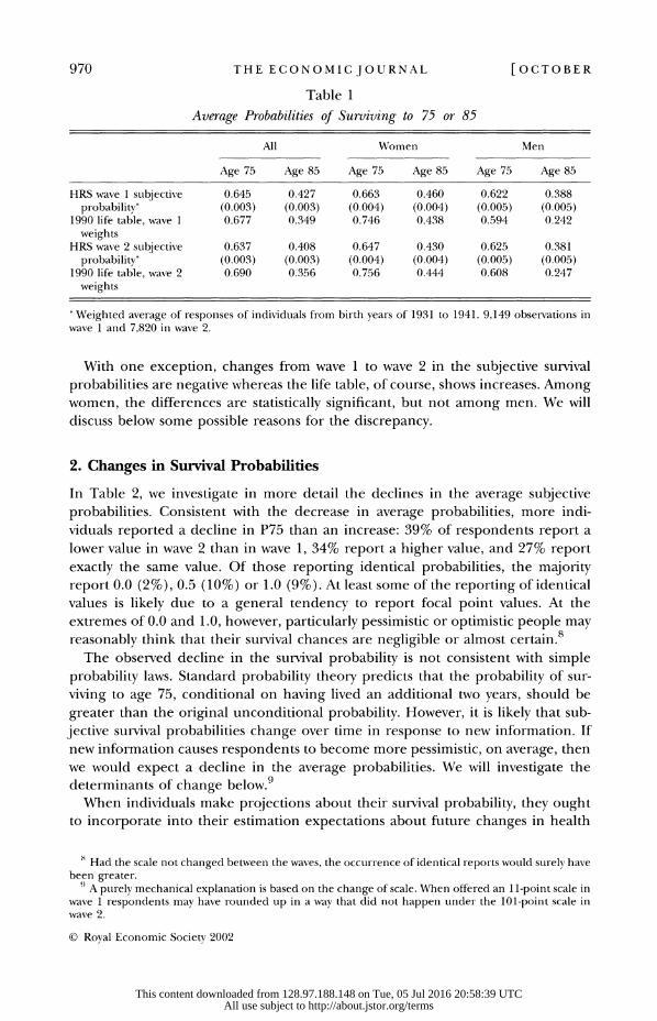
Despite these expected differences, the average subjective survival probabilities

in each wave are close to the life table averages, particularly the values for P75.6

The difference between P85 and the life table rate is substantially greater than that

for P75, implying that respondents overestimate the conditional probability of

survival to 85 given survival to 75.7 Women give higher average probabilities than

men, as- they should, although the differences are smaller than the life table dif-

ferences. A possible explanation is that when forming expectations, individuals

take into account the actual mortality experience of those around them, including

both men and women, and fail to adjust fully for differences between the sexes.

Extensive analyses of other cross-sectional patterns have been carried out in

Hurd and McGarry (1995) and Schoenbaum (1997) and we refer the interested

reader to those articles. The general conclusion to be drawn from these efforts is

that reported probabilities vary with known risk factors such as smoking, and show

the expected differences with respect to indicators of socio-economic status.

Subjective survival probabilities increase with income, wealth and schooling, are

lower for nonwhites than for whites, and are lower for those who smoke. We have

verified that these patterns continue to hold in wave 2 of the HRS, but do not

discuss the results here. However, several of the comparisons for the wave 2 data

are reported in the appendix, Table Al.

6; The response rate on the question about survival to age 75 was 98.3% in wave 1 and 97.4% in wave 2. There was little difference in the response rate in wave 1 according to whether the responident died between waves 1 and 2. High response rates to queries about subjective probabilities are in contrast to the low response rates on questions about expectations (Hurd and McGarry, 1995) eg expected age at retirenment.

7 Hamermesh (1985) finds similar results with individuals slightly Lunderestimating short-term sunrival probabilities and over-estimating longer-term probabilities relative to life table values. He views this over-estimate as possible evidence that individuals 'extrapolate past increases in longevity' (p. 393).

(? Royal Economic Society 2002



Table 1

Average Probabilities of Surviving to 75 or 85

All Women Men

Age 75 Age 85 Age 75 Age 85 Age 75 Age 85

HRS wave 1 subjective 0.645 0.427 0.663 0.460 0.622 0.388 probability* (0.003) (0.003) (0.004) (0.004) (0.005) (0.005)

1990 life table, wave 1 0.677 0.349 0.746 0.438 0.594 0.242 weights

HRS wave 2 subjective 0.637 0.408 0.647 0.430 0.625 0.381 probability* (0.003) (0.003) (0.004) (0.004) (0.005) (0.005)

1990 life table, wave 2 0.690 0.356 0.756 0.444 0.608 0.247 weights

Weighted average of responses of individuals from birth years of 1931 to 1941. 9,149 observations in wave 1 and 7,820 in wave 2.

With one exception, changes from wave 1 to wave 2 in the subjective survival

probabilities are negative whereas the life table, of course, shows increases. Among

women, the differences are statistically significant, but not among men. We will

discuss below some possible reasons for the discrepancy.

2. Changes in Survival Probabilities

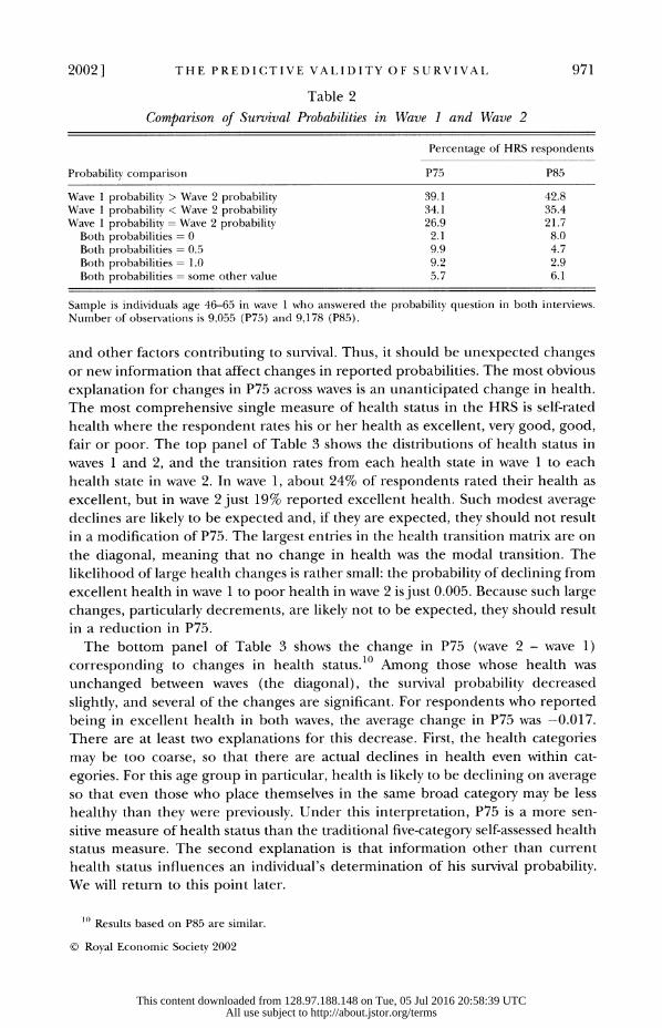
In Table 2, we investigate in more detail the declines in the average subjective

probabilities. Consistent with the decrease in average probabilities, more indi-

viduals reported a decline in P75 than an increase: 39% of respondents report a

lower value in wave 2 than in wave 1, 34% report a higher value, and 27% report

exactly the same value. Of those reporting identical probabilities, the majority

report 0.0 (2%), 0.5 (10%) or 1.0 (9%). At least some of the reporting of identical

values is likely due to a general tendency to report focal point values. At the

extremes of 0.0 and 1.0, however, particularly pessimistic or optimistic people may

reasonably think that their survival chances are negligible or almost certain.8

The observed decline in the survival probability is not consistent with simple

probability laws. Standard probability theory predicts that the probability of sur-

viving to age 75, conditional on having lived an additional two years, should be

greater than the original unconditional probability. However, it is likely that sub-

jective survival probabilities change over time in response to new information. If

new information causes respondents to become more pessimistic, on average, then

we would expect a decline in the average probabilities. We will investigate the

determinants of change below.9 When individuals make projections about their survival probability, they ought

to incorporate into their estimation expectations about future changes in health

8 Had the scale not changed between the waves, the occurrence of identical reports would surely have been greater.

) A purely mechanical explanation is based on the change of scale. When offered an 1 1-point scale in wave 1 respondents may have rounded up in a way that did not happen under the 101-point scale in wave 2.




Table 2

Comparison of Survival Probabilities in Wave 1 and Wave 2

Percentage of HRS respondents

Probability comparison P75 P85

Wave 1 probability > Wave 2 probability 39.1 42.8 Wave 1 probability < Wave 2 probability 34.1 35.4 Wave 1 probability = Wave 2 probability 26.9 21.7 Both probabilities = 0 2.1 8.0 Both probabilities = 0.5 9.9 4.7 Both probabilities= 1.0 9.2 2.9 Both probabilities = some other value 5.7 6.1

Sample is individuals age 46-65 in wave 1 who answered the probability question in both interviews. Number of observations is 9,055 (P75) and 9,178 (P85).

and other factors contributing to survival. Thus, it should be unexpected changes

or new information that affect changes in reported probabilities. The most obvious

explanation for changes in P75 across waves is an unanticipated change in health.

The most comprehensive single measure of health status in the HRS is self-rated

health where the respondent rates his or her health as excellent, very good, good,

fair or poor. The top panel of Table 3 shows the distributions of health status in

waves 1 and 2, and the transition rates from each health state in wave 1 to each

health state in wave 2. In wave 1, about 24% of respondents rated their health as

excellent, but in wave 2 just 19% reported excellent health. Such modest average

declines are likely to be expected and, if they are expected, they should not result

in a modification of P75. The largest entries in the health transition matrix are on

the diagonal, meaning that no change in health was the modal transition. The

likelihood of large health changes is rather small: the probability of declining from

excellent health in wave 1 to poor health in wave 2 is just 0.005. Because such large

changes, particularly decrements, are likely not to be expected, they should result

in a reduction in P75.

The bottom panel of Table 3 shows the change in P75 (wave 2 - wave 1) corresponding to changes in health status.10 Among those whose health was

unchanged between waves (the diagonal), the survival probability decreased

slightly, and several of the changes are significant. For respondents who reported

being in excellent health in both waves, the average change in P75 was -0.017. There are at least two explanations for this decrease. First, the health categories

may be too coarse, so that there are actual declines in health even within cat-

egories. For this age group in particular, health is likely to be declining on average

so that even those who place themselves in the same broad category may be less

healthy than they were previously. Under this interpretation, P75 is a more sen- sitive measure of health status than the traditional five-category self-assessed health

status measure. The second explanation is that information other than current

health status influences an individual's determination of his survival probability.

We will return to this point later.

1( Results based on P85 are similar.

? Royal Economic Society 2002



Table 3

Health Transition Probabilities and Changes in Subjective Survival to Age 75

(wave 2 - wave 1)

Health in wave 1

Health in wave 2 Excellent Very good Good Fair Poor

Transition probabilities Wave 2 distribution

E-xcellent 0.539 0.157 0.053 0.023 0.012 0.192 Very good 0.332 0.526 0.241 0.062 0.014 0.309 Good 0.107 0.262 0.522 0.273 0.087 0.287 Fair 0.017 0.046 0.154 0.500 0.320 0.145 Poor 0.005 0.009 0.029 0.142 0.567 0.066 Wave 1 distribution 0.237 0.294 0.276 0.129 0.064 1.000

Chiange in survival probabilities WEave 2 observations

Excellent -0.017 0.007 -0.002 0.188* 0.005 1,740 Very good -0.026* -0.021* -0.000 0.062 -0.077 2,794 Good -0.027 -0.036* 0.003 0.020 0.142* 2,601 Fair -0.029 -0.094* -0.038* -0.007 0.047 1,313 Poor -0.241 -0.220* -0.158* -0.062* -0.016 600 All -0.022* -0.025* -0.008 0.002* 0.018 Wave 1 observations 2,142 2,663 2,495 1,170 578

Denotes significance at the 5% level.

Sample is those aged 46-65 in wave 1 and reporting P75 and health status in both waves. Average change in survival probabilities (wave 2 - wave 1) was -0.014. 9,048 observations.

Below the diagonal in Table 2, health worsened between the waves and, in all

cases, P75 decreased as well. Some of the declines were very large, especially those associated with a decline to poor health. For example, among those who were in

good health in wave 1 and in poor health in wave 2, the average subjective survival

probability declined by 0.158. Entries above the diagonal correspond to an im-

provement in health, and with one exception (the transition from poor to very

good) the changes in P75 were positive. For example, among those who reported being in fair health in wave 1 and excellent health in wave 2, the survival probability increased by 0.188.

These findings are qualitatively the same as we have found in cross-section, but quantitatively the cross-section relationships are larger. This difference is to be

expected in that additional factors that influence P75 vary in cross-section but not

in panel. An unexpected decline in health from very good to poor is not accom-

panied by changes in many of the risk factors that may vary across individuals who

differ in health. Education is a good example: individuals with little education tend

to have worse health, and education has predictive power for survival. In Table 3, the change in P75 associated with a transition from very good to poor health is -0.220; in cross-section, this difference in health is associated with a difference in

P75 of -0.32 (Hurd and McGarry, 1995, Table 6). This kind of difference holds for all comparisons based on the significant effects in Table 3: the cross-section

difference in P75 is 0.05 to 0.12 greater than the panel difference. We conclude that the relationship between health change in the panel and the

change in the survival probability accords qualitatively with our expectations: those

? Royal Economic Societv 2002



whose health status worsened lowered their probability of survival while those with

an improvement in health increased their survival probability.

Although there is a clear path from the onset of diseases to self-assessed health

and to survival probabilities, the survival probabilities ought, in addition, to be

affected by events that change survival chances but not current health. To study

this difference between self-assessed health and subjective survival probabilities, we

estimated changes in subjective survival probabilities as a function of new health

information as well as other information that ought to affect survival but not

current health.

Analysis of changes rather than levels also allows us to control for unobserved

differences across individuals. In cross-sections, P75 and P85 vary in reasonable ways

with a number of observable characteristics, such as the frequency of exercise, dis-

ease conditions and smoking status (Hurd and McGarry, 1995). However, this kind

of variation does not imply causality. It may be that there exist unobserved measures

of healthiness and optimism that are correlated with both reported life expectancy

and with observable characteristics. In the panel, we can specify a relationship that

can more reasonably be interpreted to be causal because we can relate changes in

the subjective survival probability to changes in observable characteristics that are at

least partly unexpected, for example the death of a parent or the onset of disease." We recognise that the amount of new information in those events could vary

from person to person. For example, were we to query respondents about the

probability of the onset of cancer, we would likely find variation in such prob-

abilities. To the extent that these probabilities predict actual onset of cancer, the

amount of new information in actual onset will vary from person to person and,

hence, the effect of the onset of cancer on P75 will vary. Were we to have obser-

vations on the subjective probability of the onset of cancer, we could verify this

observation. However, we do not, and so it is an empirical question about the

magnitude of the revision of P75 that will acommpany an onset.

Because the left-hand variable can take only values lying between -1 and +1,

we use a variant of a logistic transformation to restrict the predicted values to this

range, and estimate the model by nonlinear least squares. The equation we esti-

mate is

e- x13

AP75 = 1 - 2 exfl

Table 4 has the coefficients and standard errors from the regression of the

changes in P75 and P85 (wave 2 - wave 1) on changes in the survivorship of the

respondent's parents, spouse and siblings, and on onset of disease conditions. The

average change in P75 was -0.014 and the change in P85 was -0.022. Table 4 also

shows the estimated effects on P75 and P85 (the derivatives). They are found by evaluating AP75 at its mean. 12

In an ordinary least squares framework, this would be a first-differenced regression controlling for individual effects.

l We obtain nearly identical results from linear estimation in terms of the derivatives in Table 4 and the significance levels.




Table 4

Nonlinear Regression of the Change in the Subjective Survival Probability (wave 2 - wave 1)

Right-hand variables Surviving to 75 Surviving to 85

Description Mean Coeff Std Err Deriv Coeff Std Err Deriv

Mother died between waves Age at death < 75 0.005 -0.242* 0.087 -0.121 -0.401* 0.143 -0.200 75 <= age at death < 85 0.021 -0.027 0.050 -0.014 -0.153* 0.054 -0.076 85 <= age at death 0.016 -0.062 0.058 -0.031 -0.144* 0.062 -0.072 Fathfr died between waves Age at death < 75 0.002 -0.251* 0.124 -0.125 -0.189 0.136 -0.094

75 <= age at death < 85 0.015 0.012 0.060 0.005 -0.004 0.064 -0.002 85 <= age at death 0.012 0.053 0.065 0.027 0.068 0.034 0.034 Respondent male and

Mother died 0.018 0.072 0.062 0.036 0.192* 0.069 0.096 Father died 0.013 0.057 0.073 0.029 -0.077 0.078 -0.038 Between waves

Spouse died 0.012 -0.173* 0.058 -0.086 -0.042 0.061 -0.021 Sibling died 0.013 -0.018 0.055 -0.009 0.003 0.044 0.002 Onset since wave 1 High blood pressure 0.042 -0.024 0.031 -0.012 -0.007 0.033 -0.003 Diabetes 0.022 0.001 0.042 0.000 -0.044 0.045 -0.022

Cancer 0.014 -0.224* 0.054 -0.112 -0.200* 0.057 -0.100 Lung disease 0.021 -0.043 0.044 -0.022 -0.044 0.046 -0.022 Heart attack 0.028 -0.052 0.040 -0.026 -0.051 0.042 -0.025 Angina 0.023 -0.035 0.045 -0.018 -0.068 0.047 -0.034 Congestive heart failture 0.012 -0.070 0.061 -0.035 -0.042 0.064 -0.021 Stroke 0.007 -0.045 0.079 -0.023 -0.090 0.080 -0.045 Arthritis 0.076 -0.015 0.023 -0.008 -0.033 0.025 -0.017 Number of observations 8512 8625 Mean of dependent variable -0.014 -0.022

' Denotes significance at the 5% level. Sample consists of individuals age 46-65 in wave 1.

The effect of a parent's death on self-assessed survival probabilities is likely to

operate through both biological and psychological mechanisms. For example, if

the parent died of a type of cancer which is known to have a genetic link, the

child might correctly reassess his own life expectancy. In addition, a parent's

death may also affect the respondent's reported probability because it reminds

him of his own mortality. We found in cross-section that the age of parents, if

alive, and their age at death, if deceased, were related to P75 and P85 but in a

more complex way than these examples suggest: if the age of a living parent or

the age at death was less than 75 or greater than 85, that age affected P75 and

P85 in approximately the same way; but if the age was greater than 75 but less

than 85, it affected them differently. For example, if a parent died at 80, it had

little effect on P75 but a substantial effect on P85. Because of this, we expect

that the death of a parent will lead to changes in the reported survival prob-

abilities, but that the change will depend on the age of the parent at death. For

example, if a parent died at age 80, it may not affect the respondent's assess-

ment of his probability of living to age 75, but could affect the probability of

living to 85.




As shown in Table 4, the death of a mother has numerically large effects on

changes in survival probabilities and the effects approximately follow the pattern

that we found in cross-section. If the respondent's mother died between waves and

was younger than 75 at her death, the respondent reduced P75 by 0.12, and P85 by

0.20. These changes are rather large given an average P75 of about 0.64 and P85 of

0.41. If the mother died at age 75 or older, the survival probability of living to age

75 was not reduced significantly, but there was a significant reduction in P85.

Apparently, respondents distinguish between P75 and P85 in a rather fine manner:

the death of a mother between 75 and 85 years of age does not affect their survival

to age 75 but it does their survival to 85. These panel changes are qualitatively

similar to the cross-section variation.

As far as P75 is concerned, the effect of a father dying is about the same as that

of a mother dying. If the death occurs when the father is younger than 75, P75 is

reduced by 0.25, but if the death is at older ages there is no significant effect.

There are no significant effects on P85 of the father dying, although if he died

before 75 the magnitude is fairly large.'3

In cross-section, the vital status of a mother or the vital status of a father had

different effects depending on the sex of a child: males focused on their fathers

and females on their mothers. Here, we allow for differing responses by sex in

each equation by including the interaction of a categorical variable indicating the

death of a mother or father with a categorical variable indicating that the re-

spondent is male. In the P75 equation, neither of the interaction terms is sig-

nificantly different from zero, although the direction of their effects is to reduce

the responsiveness of P75 to a parent's death for males in the sample. With

respect to P85, however, the interaction is substantial. The effect of a mother's

death for male respondents is significantly smaller than for females. For males, if a

mother died before age 75, the net effect is equal to -0.104 (-0.200 + 0.096). In contrast to the estimated effects of a mother's death, the effect of a father's death

is slightly larger for males than for females, although the difference is not stat-

istically significant.

Because there are no genetic links between spouses, one would expect the

impact of the death of a spouse to be largely psychological. Although the literature

on the bereavement effect has not settled on a numerical magnitude of the effects

of widowing, it does suggest that such psychological effects can have real health

influences leading to increased mortality (Korenman et al., 1997). Indeed, we find

that the death of a spouse has a large and significantly negative effect on subjective

survival to age 75. The effect on survival to age 85 is smaller, and not significantly

different from zero.14 In contrast to the effects of parental and spousal deaths, the death of a sibling has no effect in either equation, even though siblings share

- 3 The mothers of 4.2% of respondents died between waves compared to 3.0% who had a father die. Although fathers are older than mothers on average and face higher mortality rates, the more frequent

deaths of mothers result from the fact that many more respondents had a mother alive in wave 1 than had a father alive, 43% versus 19%.

14 Most of the spouses who die are male: 82 husbands died and 18 wives died. The oldest death was that of an individual who was age 85 in the first wave. Because there is less variation in the ages of spouses who die than in that of parents, we were not able to identify separate effects by age.

(?) Royal Economic Society 2002



similar genetic make-up with the respondent. Perhaps respondents are less close

psychologically to siblings than to parents or a spouse and, therefore, less affected

by the death of a sibling. Or, perhaps siblings who died at these relatively young

ages died for reasons that are less affected by genetic factors and due more to

lifestyle choices such as smoking or to accidents.

The remainder of Table 4 has effects associated with the onset of disease be-

tween the two waves. All the coefficients in each equation are negative, although

with the exception of the effects of cancer, the estimates are not significantly

different from zero, most likely becauise of the small number of new cases.15

Nonetheless, the results show that respondents reduced their subjective survival

probabilities at a new diagnosis, particularly for conditions that are more life

threatening, such as cancer.16

3. Survival Probabilities versus Health Status

Sur-vival probabilities are related to both objective and self-assessed health status

but, in principle, they also include an expectational component that is missing

from measures of health status. For example, if a respondent is healthy today but

some event occurs that increases the likelihood that he will be stricken with a

disease in the future, that event should reduce P75 and P85 but should not result

in a worsening of self-assessed health. The death of a parent may be such an

event. Except for any stress associated with the death itself, it is difficult to think

that the death could affect the respondent's current health status. Yet, depending

on the cause of death, it may increase the subjective likelihood of onset of a

genetically linked disease.17 In this section, we test this idea in our data by finding whether the death of a parent or the death of a spouse affects self-assessed health

status in the same way it affects the survival probabilities as in Table 4. Because

the health measure is categorical, we estimate a multinomial logistic model. We

defined three health states in wave 2 relative to wave 1: improved, stayed the

same, or declined. Approximately 20% of the sample had an improvement in

health, 53% had no change, and 27% had a worsening of health. A positive

coefficient from the multinomial logistic estimates means that the variable in-

creases the probability of the corresponding health change. If a parent's death

resulted in a worsening of the respondent's self-assessed health, the coefficients

under 'health better' should be negative and the coefficients under 'health

worse' should be positive.

15 The number of new cases is small: for example, about 115 respondents were newly diagnosed with cancer, and 233 with heart conditions. If all conditions other than cancer are combined into one measure of 'other disease conditions', they affect P75 significantly at the 10% level, and P85 at the 1% level. The effect of cancer on P75 and P85 is unchanged.

1 Because the survival curve increases with age, we estimated a number of more complex speci- fications that incltuded the respondent's age and age interactions. Our thought wvas that the effect of new information might have differing effects on survival depending on age. We found, however, that the simpler specification as reported in Table 4 adequately represent the data, and so we do not report the more complex estimations.

17 Data on the cause of the parent's death wotuld help to inform these issues, btut those data are not in the HRS.




We find no evidence of this effect (Table 5). For example, if the mother died

between the waves and her age at death was less than 75, the respondent was more

likely to have an improvement in health between waves (coefficient of 0.367) and

more likely to have a worsening in health (coefficient of 0.520), than to have stable

health status, although neither of the coefficient estimates is significantly different

from zero. If the mother died between the ages of 75 and 85, the probability of an

improvement in health fell and the probability of worsening of health increased

but the effects are not significant. Nearly all coefficients for the death of a father

act to reduce the probability of changing states, and none is significantly different

from zero. The death of a spouse increased the probability of an improvement in

health status and decreased the probability of a worsening of status, but the effects

are not significant.'8 In contrast to these weak and contradictory effects, the onset of a disease affects

current health status in the expected manner. The coefficients on the disease

measures typically increase (significantly) the probability of moving to worse

Table 5

Multinomial Logit Coefficients: health better (20%) or worse (27%) versus same (53%)

Health better Health worse

Variable Coefficient Std Err Coefficient Std Err

Mother died between wzaves Age at death < 75 0.367 0.396 0.520 0.336 75 <= age at death < 85 -0.367 0.249 0.061 0.193 85 <= age at death 0.161 0.259 0.051 0.231 Father died between wavies Age at death < 75 -1.036 0.760 -0.527 0.531 75 <= age at death < 85 -0.228 0.293 -0.082 0.244 85 <= age at death -0.395 0.334 0.175 0.250 Respondent male and Mother died -0.537 0.311 -0.114 0.242 Father died -0.227 0.380 0.044 0.288 Other deaths

Spotuse died 0.234 0.234 -0.289 0.252 Sibling died 0.000 0.247 -0.036 0.224 Since wave 1 diag-nosed zvith High blood pressure 0.146 0.143 0.619* 0.115 Diabetes 0.197 0.187 0.341* 0.162 Cancer -0.073 0.313 1.272* 0.202 Lting disease -0.495* 0.234 0.192 0.163 Heart attack -0.036 0.208 0.936* 0.146 Angina -0.110 0.205 -0.391 0.179 Congestive heart failure -0.567 0.325 -0.228 0.233 Stroke -0.218 0.405 0.728* 0.270 Ai-thritis -0.050 0.109 0.364* 0.089

A positive coefficient increases the probability of a health change. Number of observations 8,545.

Denote significance at a 5% level. Sample is individuals 46-65 in wave 1.

18 We also estimated an ordered logistic model for change in health status where the change was meastured as the difference between wave 2 status and wave I stattus, and health was measured on a scale of 1-5 in each period. The variables indicating parental mortality were not significantly different from zero either individually or as a group.




Table 6

Means of Subjective Survival Probabilities by Survivorship to Wave 2

Died between waves Lived to wave 2 Survivorship unknown

Variable Mean Std Err Mean Std Err Mean Std Err

Prob live to 75 0.45 0.03 0.65 0.00 0.66 0.02 Prob live to 85 0.28 0.02 0.43 0.00 0.42 0.02 Number of 183 10,642 265

observations

Sample is individuals 46-65 in wave 1.

health and, in most cases, decrease the probability of improved health, or else have

no significant effect.

Because diseases lower both reported health status and the reported survival

probability, while the death of a parent or of a spouse significantly lowers only the

reported values of P75 and P85, we conclude that the subjective survival prob-

abilities measure more than health status: they have an expectational component

as well as a health-status component.

4. Mortality Outcomes

4.1. The Predictive Pozver of Subjective Probabilities of Survival

We have shown that individuals update their expectations in reasonable ways in

response to new information. We now ask whether the survival probabilities

predict actual mortality. In our sample of 11,090 wave 1 respondents, 183 died

between wave 1 and wave 2, 10,642 survived, and the vital status of 265 others was

unknown at wave 2.19 When weighted, these figures yield a mortality rate of 0.0169. Table 6 presents the inean subjective survival probability for each group as re-

ported in the first wave. Those who died reported an average P75 of 0.45 compared

to 0.65 for those who survived. Thus, at least in a gross way, the subjective survival

probabilities predict mortality.20 Figure 1 shows the cumulative distributions of P75 for those who died compared

with those who survived. Not only is the average different for these two groups, but

the differences persist throughout the distributions. For example, about 11% of

those who survived reported P75 to be 0.40 or less whereas 43% of those who died

gave a value of 0.40 or less; the medians are 0.70 and 0.50.

Figure 2 shows two-year mortality rates as a function of P75 and P85. Mortality

rates decline almost monotonically as P75 varies from 0.1 to 1.0. Although there

19 The unknown category consists of those respondents who could not be located in the second wave of the survey and whose vital status could not otherwise be ascertained.

20 Even were P75 to give accurate predictions of survival to age 75, it would not necessarily predict two-year survival. We could imagine a risk factor that is negligible over a short-term but has long-term cumulative effects, for example the take-up of smoking. Apparently, P75 does predict short-term mortality, but we will have to wait uintil a cohort reaches age 75 to find how well quantitatively it predicts survival to 75. Given its association with short-term survival, it would be surprising if it did not predict at least qualitatively survival to 75.




Cumulative distributions

Based on 10608 observations 0.8

0.6

0.4

0 0 0.1 0.2 0.3 0.4 0.5 0.6 0.7 0.8 0.9

Subjective survival to 75

~:: ~ i Survived Died

Fig. 1. Subjective survival

0.08

based on 10608 observations

0.06

0 .0 4 ...---- ...

0.0

0 0 1 2 3 4 5 6 7 8 9 10

Subjective survival probability

Fig. 2. Two-year mortality rates

?D Royal Economic Society 2002



was substantial bunching of responses at 0.5 in each wave (21.2% in wave 1, not

shown), the mortality rate at 0.5 is not noticeably different from mortality rates in

the range of 0.3 to 0.7, suggesting that respondents who report a value of 0.5 are

drawn from nearby probability points. Mortality at zero is greater than at any other

point except 0.1. The fact that it is lower than at 0.1 suggests reporting error by

some respondents.21 Some individuals who answered with a zero did, in fact, have high mortality risk, but some may not have understood the probability question or

simply gave a convenient focal response. Therefore, the responses at zero are a

mixture of a high mortality rate for one group and a rate perhaps closer to average

for another group.

The risk curve for P85 is considerably shallower, and even has an increase from

0.7 to 1.0. An implication is that P85 contains more observation error than P75.

This implication is consistent with the results in Table 1 where the average of P85

was considerably higher than the life table average.

We now examine how well the subjective survival probability at wave 1 predicts

actual mortality for our sample of individuals age 46-65 whose mortality status is

known. We estimate a logistic model where the left-hand side variable is equal to

one if the individual died between waves and zero if he survived. The explanatory

variables include P75 and other factors that ought to be correlated with mortality

such as income, wealth, schooling, smoking behaviour and disease conditions. The

first set of results in Table 7 reports the coefficient estimates, standard errors, and

probability derivatives for this specification.22

The coefficient on P75 is significantly different from zero and fairly large. An

increase in the probability from zero to 1.0 reduces the mortality hazard by 0.016,

which is equal to the average mortality hazard. In a mortality model such as a

proportional hazards model, this change would increase considerably the likeli-

hood of survivorship to advanced age.

Mortality falls with income, but the effects are significantly different from zero

only at the 6% level. A $100,000 increase in income decreases the mortality probability by 0.01 percentage points. The effects of wealth are smaller in mag-

nitude and neither term is significantly different from zero. As one would expect,

mortality increases significantly with age: the difference between the risk of a

51-year-old and a 61-year-old is about 0.01. Marital status per se has only a small

negative effect. Apparently, the strong difference by marital status typically

observed in data is in part the result of differences in other variables that are

correlated with marital status such as disease conditions. Men have mortality rates

about 0.009 higher than women, which is about the same as would be found in a

life table for people of the HRS age range. Thus, even controlling for a large

number of covariates does not reduce the male-female mortality differential.

Whites have lower mortality rates than non-whites after controlling for other risk

factors and the effect is significantly different from zero at the 10% level. Smoking

increases the mortality rate by over 75%, even after controlling for many other risk

21 The difference is not statistically significanit, however. 22 The reported derivatives are mean values calculated over all observations in the sample.

(D Royal Economic Society 2002



Table 7

Logit Estimates of the Determinants of Mortality, wave 1 to wave 2

Excluding Health Including Health

Coeff Std Err Deriv Coeff Std Err Deriv

Probability live to age 75 -1.031** 0.253 -0.016 -0.598** 0.260 -0.009 Health Status

Excellent (omitted) - - - Very good 0.157 0.371 0.002 Good 0.408 0.352 0.006 Fair 1.097** 0.363 0.016 Poor 1.754** 0.384 0.026 Financial Measures

Income (in $100,000s) -0.693* 0.364 -0.011 -0.423 0.360 -0.006 Inconme squared 0.081** 0.031 0.001 0.059* 0.031 0.001 Wealth (in $100,000s) -0.373 0.494 -0.006 -0.125 0.510 -0.002 Wealth squared 0.051 0.115 0.001 0.004 0.127 0.000 Demographic Characteristics Age 0.051** 0.021 0.001 0.052** 0.021 0.001

Married -0.282 0.185 -0.004 -0.265 0.186 -0.004 Male 0.566** 0.178 0.009 0.517** 0.179 0.008 Noinwhite 0.338* 0.189 0.005 0.275 0.191 0.004 Schooling Less than 12 -0.033 0.185 -0.001 -0.187 0.188 -0.003 Equal to 12 (omitted) - - - - - More than 12 -0.325 0.215 -0.005 -0.266 0.217 -0.004 Disease Conditions

High blood pressure 0.195 0.169 0.003 0.081 0.172 0.001 Diabetes 0.547** 0.193 0.008 0.335* 0.196 0.005 Cancer/tumor 1.650** 0.200 0.025 1.488** 0.203 0.022 Lung disease 0.256 0.221 0.004 0.037 0.222 0.001 Ever heart attack 0.671** 0.212 0.010 0.519** 0.217 0.008 Angina -0.359 0.294 -0.006 -0.516* 0.293 -0.008

Congestive heart failure 0.727** 0.306 0.011 0.562* 0.305 0.008 Stroke 0.707** 0.265 0.011 0.495* 0.265 0.007 Arthritis/rheumatism -0.124 0.166 -0.002 -0.277 0.169 -0.004 Other Health Measures Smoker 0.861** 0.230 0.013 0.835** 0.231 0.012 Former smoker 0.580** 0.227 0.009 0.587** 0.227 0.009 Never smoked (omitted) - - - - - BMI low 0.422 0.259 0.006 0.256 0.263 0.004 BMI high 0.271 0.230 0.004 0.183 0.231 0.003 Number of observations 10,484 10,479

** Denotes significance at the 5% level, * denotes significance at the 10% level.

factors. Former smokers also have an elevated risk, with a mortality rate that is

about 53% higher than non-smokers.23 Among the disease conditions, cancer is the strongest predictor of mortality,

increasing the two-year mortality rate by 150%. The reports on the subjective

survival probabilities are consistent with this result: in Table 4, a new cancer had

the largest effect among the disease conditions on reducing the subjective survival

probability. In a similar way, having had a heart attack, heart failure and having

23 Apparently former smokers do not recognise their higher mortality rate: as shown in Table 4, former smokers report P75 to be the same as non-smokers.




Table 8

Weighted Number of Observations and Two-year Mortality Rate, born 1931-41

All Females Males

Survived to wave 2 7212.5 3821.8 3390.8 Died before wave 2 112.5 45.5 67.0 Survivorship unknown 177.75 96.8 81.0 Mortality rate

HRS estimate* 0.0154 (0.0013) 0.0118 (0.0015) 0.0194 (0.0021) Adjustments

Imputed mortality for nmissing 0.0155 0.0119 0.0196 Mean time between interviews 0.0165 0.0127 0.0209 1993 Life table 0.0167 0.0125 0.0214

* Life table estimate is weighted average (HRS weights) of single-age mortality rates from 1990 and 2000 life tables (Bell et al., 1992) interpolated to 1993. Sample consists of those born in the years 1931-41 and weighted to account for over-sampling of blacks, Hispanics and Floridians.

had a stroke all increase mortality risk by approximately 65%. New diagnoses of

heart attack and heart failure are strong determinants of a decline in the subjective

survival probability in Table 4.

Even though a number of explanatory variables are significant, the model does

not explain much of the variation in mortality outcomes: the pseudo R2 is just 0.025.24 Adding P75 to the other variables shown in the table increases the pseudo R2 by 7%.

Some may find it natural to think of the subjective survival probabilities as an

alternative measure of overall health. To test whether the survival probabilities

provide information beyond that contained in reported health status, we re-esti-

mated the logistic model and included the subjective health measures from wave 1

as measured by four categorical health indicators as very good, good, fair or poor.

(Excellent health is the omitted category.)

As shown in the second set of results in Table 7, P75 continues to have a negative and significant effect on the mortality probability, although the magnitude of the

effect is reduced by half. A change in P75 from 0 to 1 increases the probability of dying between waves by 0.009. These results indicate that the subjective probability

contains information in addition to subjective health as measured by the five-point

scale, and it is reasonable to interpret it as an expectational component. The

effects of the other variables are either attenuated or not altered. For example,

among the disease conditions, cancer continues to have the largest effect, and the

magnitude is reduced only slightly from the first set of estimates. Adding the four

health variables increases the pseudo R2 by 14%.

4.2. Comparisons with Life Table Probabilities

As a check on the representativeness of the HRS mortality rates, we compare the

mortality experience of the HRS respondents to mortality rates calculated from life

24 Calculated as 1 - exp[2/n(In Lo - in LI] where In Lo is the log likelihood based only on the constant and In 1I is the log likelihood based on the constant and explanatory variables.




tables. To make a meaningful population comparison, we restrict our sample to

respondents born from 1931 to 1941, but include those with proxy responses

whom we excluded previously. Table 8 shows the mortality experience of the wave 1

sample.25 The estimated mortality rate from this sample is 0.0154, somewhat lower

than the mortality rate of 0.0167 calculated from the life tables.26 For women and

for men, the rates from the HRS are 0.0118 and 0.0194, compared with 0.0125 and

0.0214 from population life tables.

However, this comparison ignores the mortality experience of those in the

sample whose survival status is unknown. It is likely that those who are lost to

follow-up in the survey have a higher than average mortality risk. If this were true,

their inclusion would increase the average HRS mortality rate. We can use esti-

mates from the logistic model of mortality to predict average mortality for the

missing respondents, and adjust the overall mortality rate of the wave 1 sample

accordingly. Using the wave 1 values of the explanatory variables for the missing

cases, we predict their average two-year mortality rate to be 0.021, which is

approximately 40% higher than the mortality rate of the 51-61-year-olds in the

wave 1 sample whose survivorship is known. Based on this estimate, we can adjust

upward the total mortality rate of the wave 1 sample from 0.0154 as shown in

Table 8 to 0.0155.27

This estimate is still slightly lower than that calculated from life tables. There are

two explanations for the consistently lower mortality among HRS respondents. At

baseline, the HRS is representative of the non-institutional population. Those in

institutions likely have higher mortality risk than the non-institutionalised popu-

lation, but we have no good way to account for the institutionalised population.

Second, the time span between waves 1 and 2 is not exactly two years. The mean

interval is 22.5 months, and the modal interval is 22 months. Normalising to

24 months increases the two-year mortality rate to 0.0165, very close to the life table

rate. Note that, as with the reported survival probabilities, there is a difference by

sex in the agreement between life table numbers and the values from the HRS

sample. Whereas women in the HRS appear to underestimate their survival

probability (Table 1), they also died at greater than expected rates. Similarly, while

men apparently overestimated survival probabilities relative to life table values,

their actual mortality experience was lower than what one would have predicted.

This difference is likely due, at least in part, to selection of the sample. A greater

fraction of men of this age group (51-61 years old) are in institutions than women.

By omitting the institutionalised population, HRS has omitted more institution-

alised men than women. Thus, observed mortality rates of men in the sample

would be expected to be biased downward relative to the population rates to a

greater degree than for women.

25 The counts are weighted to control for the over-sampling of blacks, Hispanics and Floridians. 2(i We obtain our life table mortality rates for 1993 by interpolating between a 1990 and a 2000 life

table.

27 Note that this adjustment does not include the few proxy respondents whose survival status is unknown. Because these respondents were not asked about P75, we cannot impute a survival probability for this group.




A second reason for the difference could be from the forward-looking nature of

the subjective survival probabilities: if respondents observe improvements in their

health and in their future health prospects, they ought to revise upward their

survival chances. A period life table is based on mortality at a point in time, and

there will be a lag before health improvements are reflected in it. Of course, a

period life table does not reflect expected improvements in health. Perhaps men

observed that their health and health prospects had improved, and they stated

these observations when they reported their subjective survival probabilities. Their

improved health status resulted in actual mortality rates that are lower than those

found in life tables.

5. Conclusion

Respondents can and will answer questions about subjective probabilities, and the

response rates to such questions are very high. Previous research has established

that the survival probabilities aggregate to averages that are close to life table

averages, and that they covary with risk factors in a way that suggests that they will

predict actual mortality. The objectives of this paper are to find how subjective

probabilities evolve in response to new information and how well they predict

mortality. These are essential steps before we can have confidence in their use to

explain behaviour.

We found that subjective survival probabilities decline with the death of a par-

ent, but that self-assessed health is not affected. We interpret this to mean that the

subjective survival probabilities have an expectational element and that they are

not simply an alternative measure of health status. Furthermore, the survival

probabilities predict mortality. Those who survived from wave 1 to wave 2 of the

HRS gave subjective survival probabilities in wave 1 that were about 50% higher

than those who died between the waves. This predictive power remains even when

self-assessed health status is controlled for.

We expect that these survival probabilities will prove to be useful as explanatory

variables in economic models. For example, in life-cycle models, individual-specific

mortality probabilities could be used to produce better estimates of the deter-

minants of an individual's consumption and wealth trajectories. Their inclusion

may help to explain apparent inconsistences and anomalies in data, such as in-

creasing wealth during retirement and seemingly inadequate savings by some in-

dividuals before retirement: in the first case, some individuals may expect to be

exceptionally long-lived and, in the second, they may have such small subjective

survival chances that saving is not called for.

RAND and NBER

University of California, Los Angeles and NBER

Date of receipt offirst submission: December 1998 Date of receipt of final typescript: September 2001




Appendix

Table Al

Average Subjective Probability of Surviving to Age 75, Wave 2

Prob live to 75 Prob live to 85

Characteristic Prob Std Err Prob Std Err

Income quartile

Lowest 0.583 0.007 0.391 0.007 Second 0.621 0.006 0.389 0.006 Third 0.650 0.006 0.418 0.006 Highest 0.685 0.005 0.444 0.006 Wealth quartile

Lowest 0.573 0.007 0.377 0.007 Second 0.617 0.006 0.394 0.006 Third 0.645 0.006 0.415 0.006 Highest 0.698 0.005 0.452 0.006 Schooling Less than high school 0.560 0.007 0.367 0.007 High school graduate 0.634 0.005 0.397 0.005 College graduate 0.687 0.004 0.454 0.005 Smoking behaviour

Never smoked 0.659 0.005 0.437 0.005 Smoked but quiit 0.657 0.005 0.416 0.005 Current smoker 0.586 0.007 0.368 0.007

Sample is individuals aged 46-65 in wave 1. Based on approximately 9159 observations from wave 2. Number varies by characteristic due to missing values of characteristics.

References

Bell, Felicity C., Wade, Alice H. and Goss, Stephen C. (1992). 'Life tables for the United States social

security area 1900-2080', SSA Publication 11-11536, Social Security Administration, Washington, D.C.

Bernheim, B. Douglas (1989). 'The timing of retirement: a comparison of expectations and realizations',

in (David Wise, ed.), The Economics of Aging, Chicago: The University of Chicago Press, pp. 335-55. Bernheim, B. Douglas (1990). 'How do the elderly form expectations: an analysis of responses to new

information', in (David Wise, ed.), Issues in the Economics of Aging, Chicago: The University of Chicago Press, pp. 259-83

Domninitz, Jeffery (1998). 'Earnings expectations, revisions and realizations', The Review of Economics and

Statistics, vol. 80 (3), pp. 374-88. Dominitz, Jeffery and Manski, Charles (1997). 'Using expectations data to study subjective income

expectations', Journal of the American Statistical Association, vol. 92 (439), pp. 855-62. Hamermesh, Daniel S. (1985). 'Expectations, life expectancy, and economic behavior', QuarterlyJournal

of Economics, vol. 100 (2), pp. 389-408.

Hamermesh, Daniel S. and Hamermesh, Frances W. (1983). 'Does perception of life expectancy reflect

health knowledge?', American Journal of Public Health, vol. 73 (8), pp. 911-4. Hurd, Michael D., McFadden, Dan and Gan, Li (1998), 'Subjective survival curves and life cycle behavior', in

(David Wise, ed.), Inquiries in theEconomics ofAging, Chicago: University of Chicago Press, pp. 259-305. Hurd, Michael D. and McGarry, Kathleen (1993). 'The relationship between job characteristics and

retirement', NBER working paper no. 4558.

Hurd, Michael D. and McGarry, Kathleen (1995). 'Evaluation of the subjective probabilities of survival in the health and retirement study', journal of Human Resources, vol. 30, pp. s268-92.

Hurd, Michael D. and McGarry, Kathleen (1996). 'Prospective retirement: effects ofjob characteristics, pensions, and health insurance', mimeo, University of California, Los Angeles.

Juster, F. Thomas and Suzman, Richard (1995). 'An overview of the health and retirement study', Journal of Human Resources, vol. 40, pp. s7-56.

Korenman, Sanders, Goldman, Noreen and Fu, Haishan (1997). 'Misclassification bias in estimates of

bereavement effects', Amencan Journal of Epidemioloqy, vol. 145 (11), pp. 995-1002. Manski, Charles F. (1990). 'The use of intentions data to predict behavior: a best case analysis',Journal of

the American Statistical Association, vol. 85, pp. 934-40. Schoenbaum, Michael (1997). 'Do smokers understand the mortality effects of smoking: evidence fi-om

the health and retirement sturvey', American Journal of Public Health, vol. 87 (5), pp. 755-9.

?D Royal Economic Society 2002


Documents

The Predictive Validity of Subjective Probabilities of ... Hurd.pdf · The Predictive Validity of Subjective Probabilities of Survival ... actual income to understand better the income