Embed Size (px)
Citation preview
THE PREDICTIVE POWER OF YIELD CURVE FOR OUTPUT AND INFLATION IN THAILAND
YUWANEE OUINONG Faculty of Economics, Thammasat University
ABSTRACT
The attention on yield curve as a predictor of economic activity has been continuously increasing many researchers. Numerous studies proved that the slope of the yield curve has valuable forecasting power on output growth and inflation. This research examines the predictive power of yield curve for output and inflation in Thailand on various time horizons ahead. In-sample forecast finds the predictive contents from 1- up to 24-month ahead for output and 6-month ahead for headline inflation. However, out-of-sample outcomes suggest that the yield spread forecasting models do not significantly outperform AR model. Constructing the spread decomposition model, this study finds that the impact of expectation effect is more significant than term premium effect in the relationship of yield curve and real economic activity.
1
1. INTRODUCTION
Concerning with growth and stability in economy, current and future information on economic activities and inflation are important to all economic agents. The policymakers, who have to make decision today, must take into account the forward-looking of the economy. They rely on various data and methods used as predictors. The attention on yield curve as a predictor of economic activity has been increasing recently by many researchers.
The slope of the yield curve, the difference in yields between long-term and short-term interest rates, has been proved by numerous researches that it has valuable forecasting power on output growth and inflation. Wheelock and Wohar (2009) have done a survey of more than 30 literatures about the prediction of output growth and recessions by the term spread, where various methods have been applied in different papers. Most of them found significant predictive content of yield curve for output growth, recession, and inflation even though many distinct models are used.
Studied by Hamilton and Kim (2002), Stock and Watson (2003), Estrella and Mishkin (1998), Estrella, Rodrigues, and Schich (2003), they found that term spreads predict output growth and recessions up to one year in advance and also found the usefulness of yield curve varies across countries and over time. Mishkin (1990), Lowe (1992) applied the classic Fisher equation to construct inflation forecasting model using the yield spread as explanatory variable. Significant relationships between those variables have been found and the result appears to be varied depending on different maturities of yield spread applied.
Even though numerous papers proposed the evidence of the term spread’s forecasting power, very few of them have done research in Asian countries, especially in Thailand. Therefore, this paper aims to investigate the predictive relationship of the term spread for economic activity and inflation in Thailand. A brief literature review here highlights the previous studies in emerging countries. Mehl (2006) found that domestic yield curves in emerging economies contained predictive content at both short and long forecast horizons. He also examined international financial linkages and found that the ability of the slope of the US or the euro area yield curve can help to predict inflation and growth in emerging economies. Another paper by Chen, Wang, and Yen (2005), they studied about the ability of the term structure to predict economic condition in G7 and Asian countries. They found that US term spreads are more important to forecast future economic growth of Asian emerging countries than domestic spreads.
For case of Thailand, the objective of this paper is to examine the predictive power of yield curve for output and inflation on various time horizons ahead. Both in-sample and out-of-sample forecast are investigated. Moreover, this research will also find marginal predictive power by comparing the effect of yield spreads with other macroeconomics variables. Basing on expectation hypothesis and term premium of term structure theory, the decomposition of why term spread helps forecast real activity is performed in the final section.
2
2. HYPOTHESIS
The slope of the yield curve (also called yield spread or term spread) is defined as the difference between long-term and short-term interest rates, which in most previous studies, was derived from the difference between long-term government bonds yield and short-term treasury bills yield.
Predictive power of the yield curve for output
The theoretical framework behind possible predictive relationship between the yield curve and output growth is based on the expectation hypothesis. Expectation hypothesis theory states that the long-term interest rate is equal to the average of expected future short-term interest rates. If the expected short-term rates were lower than the short rate today, then the long-term rate would be less than short rate. For example, suppose contractionary monetary policy results in short-term interest rates that are higher than the expected future short-term rates. Then the long rates would be lower than current short rates, which is represented by the inverted yield curve (negative yield spread). This inversion in yield curve implies lower economic activities since the low interest rate are typically associated with declining economic activity. Moreover, term-premium is another component on the hypothesis of output prediction as recommended by Hamilton and Kim (2002), however, it is assumed to be constant over time in the pure expectation hypothesis. According to the mentioned hypothesis, yield curve should contain some useful information of predicting output growth
Predictive power of the yield curve for inflation
According to the classic Fisher equation, the nominal interest rate reflects market expectations of future inflation and the real interest rate for a given maturity.
n n nt t ti rπ ≈ −
( ) ( ) ( )n m n m n mt t t t t ti i r rπ π− ≈ − − −
where π tn, it
n, rtn denote inflation rate, nominal interest rate, and real interest rate from time t to t+n
respectively. By subtracting short-term interest rate on both side of the upper equation, we obtain term spread (it
n − itm ) on the right hand side. According to the lower equation, the yield spread should have
some influence on expected changes in inflation. Therefore, the slope of the yield curve should have some content reflected in inflation.
3. DATA
The yield spread defined in this research is the difference between 10-year government bond yield and 3-month Treasury bill yield. The sample period starts from 2001, the time that short-term yield data was available, to 2013 on monthly basis. Other different term spreads, rather than 10-year and 3-month rates, are also investigated for the purpose of robustness check. All yield data is obtained from Thai Bond Market Association (ThaiBMA) which is available on daily basis, however, monthly average will be used in this research to be corresponding with time horizon of other variables.
3
Our objective is to investigate two main macroeconomics variables. The first variable is output growth represented by Manufacturing Production Index (MPI) growth from Office of Indutrial Economics (OIE), which has advantage over GDP regarding the frequency of the data. Another variable is inflation rates represented by Consumer Price Index (CPI) from Bureau of Trade and Eonomic Indices, Ministry of Commerce. Both headline and core inflation rates are examined.
Other macroeconomic variables include leading economic indicators and monetary policy measures from Bank Of Thailand (BOT). Leading economic indicators are composed of Authorized Capital of Newly Registered Companies, Construction Areas Permitted in Municipal Zone, Exports, Number of Foreign Tourists, SET index, Broad Money, and Oil Price Inverse Index. The monetary policy measures used include the policy rate (RP), growth of narrow money (M1) and broad money (M2).
4. METHODOLOGY
The analysis is divided into 3 parts, the first part starts from examining the ability of term spread to predict output and inflation in the next period as well as its usefulness beyond other independent variables. Next, out-of-sample forecast is estimated in order to clearly identify its predictive content. As previous relationships exist, the last part conducts the decomposition of yield spread to see why those predictive contents appear.
4.1 In-Sample Measure of Predictive Content
Output case
Following Estrella and Mishkin (1997), Hamilton and Kim (2002), Stock and Watson (2003) that studied similar models in forecasting output using yield spread, this research starts by a simple bivariate model using OLS that regress output growth on yield spread. The forecasting begins from next one-month up to k-month ahead in order to see the predictive power of yield curve along various time horizons. The basic model is estimated as
(1)
where represents output growth over next k months, represents term spread at time t, and represents dummy variable for the period of Thailand great flood in the last quarter of 2011.
Manufacturing Production Index (MPI) is transformed such that 𝑌!! = 1200/𝑘 ×ln (𝑀𝑃𝐼!!!/𝑀𝑃𝐼!), in which the term 1200/k is multiplied to standardize MPI growth in annualized form. From hypothesis in the previous section, the value of is expected to be positive.
Since the lagged output may be useful in forecasting the output growth, the model including those lags in addition to equation (1) will also be estimated where the number of lags will be chosen by information criteria such as AIC and SIC. Only one lag is included for case of Thailand in this paper since it is the only significant lag and this also corresponds to the suggestion by in Hamilton and Kim (2002).
In addition, other variables might have effect in predicting output as well. In order to see the marginal predictive content of spread beyond other macroeconomic variables, model (2) is estimated where more explanatory variables are added including lagged value of MPI growth, leading economic indicators, monetary measures and dummy variables for the period of great flood in 2011.
Ytk = β0 +β1Spreadt +δ0Dt +εt
Ytk Spreadt
Dt
β1

4
Leading economic indicators consist of 7 components as mention in the data part. Instead of applying all 7 variables into a regression model which can result in multicollinearity problem, the technique of principal component analysis (PCA) is performed to construct a single factor that will extract common signals from all leading indicators. As a result, only one principal component variable will be used to represent all leading economic indicators, denoted as .
(2)
Inflation case The basic model used in forecasting inflation is similar to the case of output growth, model (1).
or (3)
The preceding equation is considered as ‘inflation equation’ where we want to see the predictive content of term spread on inflation over the next k periods. However, the ‘change in inflation equation’ should also be estimated as suggested by Mishkin (1990). Based on classic Fisher equation that decomposes the nominal interest rate of given maturity into a real rate and expected inflation component,
where, = Expected inflation rate from time t to t+m
= The m-period nominal interest rate at time t.
= The m-period real interest rate at time t.
The realized inflation rate over the next m periods can be written as the expected inflation rate plus the forecast error of inflation:
, where = The forecast error of inflation = .
Substituting from classic Fisher equation, we obtain
The preceding equation can be expressed in the form of the inflation forecasting equation as follow:
However, in order to examine the predictive content of term structure, the explanatory variables on the right hand side should be the different between long-term and short-term interest
rates rather than n-period nominal rate solely. Therefore, we subtract m-period inflation rate from equation (5) to obtain
𝜋!! − 𝜋!! = 𝛽! + 𝛽! 𝑖!! − 𝑖!! + 𝜀!!,! (4)
Leadt
Ytk = β0 +β1Spreadt +δ0Dt +εt
Inflationtk = β0 +β1Spreadt +δ0Dt +εt
Etπ tn = it
n − rtn
Etπ tn
itn
rtn
π tn = Etπ t
n +εtn εt
n π tn −Etπ t
n
Etπ tn
π tn = it
n − rtn +εt
n
π tn =αn +βnit
n +ηtn
(itn − it
m ) (itn )
Ytk = β0 +β1Spreadt +β3Y
1t−1 +β4Leadt + Σi=1
cφiMonetit + Σj=1
dδ jDjt +εt
k

5
where 𝜋!!is the inflation rate from t to t+m and 𝑖!! is the nominal interest rate from t to t+m. In simply form, the above model estimates
𝐹𝑢𝑡𝑢𝑟𝑒 𝑐ℎ𝑎𝑛𝑔𝑒 𝑖𝑛 𝑖𝑛𝑓𝑙𝑎𝑡𝑖𝑜𝑛 ! = 𝛽! + 𝛽!𝑆𝑝𝑟𝑒𝑎𝑑! + 𝜀!
Both model (3) and (4) will be estimated and defined as inflation equation and inflation change equation respectively.
4.2 Out-of-Sample measure of predictive contents
In order to extend the predictive power of yield spread, out-of-sample forecasts are performed. Starting by estimation of the spread forecasting model from sample period of 2001M1 to 2012M12, then we perform the forecast of dependent variable in 2013M1 to the next 3, 6, 12, and 24 months ahead. The baseline models used for out-of-sample forecast are model (1) and model (3) for case of output growth and inflation respectively.
Root mean square error (RMSE) will be used to measure the performance of forecasting as it represents the difference between values predicted by the models and the value actually observed at that time, i.e. the accuracy of forecasting model. The predictive power of spread forecasting model would be examined by comparing RMSE of spread model against the simple AR model which includes only lagged value of the dependent variable itself as suggested by Stock and Watson (2003). The relative RMSE ratio is calculated as
𝑅𝑒𝑙𝑎𝑡𝑖𝑣𝑒 𝑅𝑀𝑆𝐸 𝑟𝑎𝑡𝑖𝑜 = 𝑅𝑀𝑆𝐸 𝑜𝑓 𝑠𝑝𝑟𝑒𝑎𝑑 𝑓𝑜𝑟𝑒𝑐𝑎𝑠𝑡𝑖𝑛𝑔 𝑚𝑜𝑑𝑒𝑙
𝑅𝑀𝑆𝐸 𝑜𝑓 𝐴𝑅 𝑚𝑜𝑑𝑒𝑙
The lower value of RMSE indicates the more accuracy of forecasting performance. Therefore, the value of relative RMSE ratio below 1 will indicate that the spread forecasting model outperforms simple AR model.
4.3 Decomposition of why the yield curve helps predict output.
As the relationship in the previous parts exists, we further examine the factors in yield spread to see why it relates to output. The decomposition of yield spread in this section will be based on expectation hypothesis theory. Since the theoretical framework of output growth and yield curve relationship is based on expectation hypothesis, only output variable will be focused in this section. Hammilton and Kim (2002) studied the decomposition of term structure and suggested that term structure of interest rates are determined by expectation of future short-rate effect and the term premium effect. As a result, the impact of term spread on output growth must be able to explained by either expectation effect or term premium effect as well.
According to expectation hypothesis, the long-term interest rate is equal to the average of expected future short-term rate plus term premium component,
6
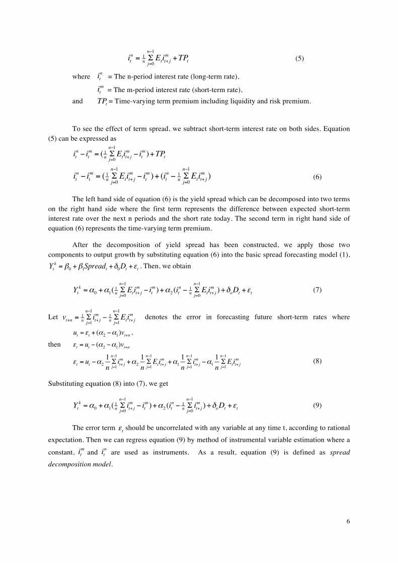
(5)
where = The n-period interest rate (long-term rate),
= The m-period interest rate (short-term rate), and = Time-varying term premium including liquidity and risk premium.
To see the effect of term spread, we subtract short-term interest rate on both sides. Equation (5) can be expressed as
(6)
The left hand side of equation (6) is the yield spread which can be decomposed into two terms on the right hand side where the first term represents the difference between expected short-term interest rate over the next n periods and the short rate today. The second term in right hand side of equation (6) represents the time-varying term premium.
After the decomposition of yield spread has been constructed, we apply those two components to output growth by substituting equation (6) into the basic spread forecasting model (1),
. Then, we obtain
(7)
Let denotes the error in forecasting future short-term rates where
, then
(8)
Substituting equation (8) into (7), we get
(9)
The error term should be uncorrelated with any variable at any time t, according to rational expectation. Then we can regress equation (9) by method of instrumental variable estimation where a
constant, and are used as instruments. As a result, equation (9) is defined as spread decomposition model.
itn = 1
n Σj=0
n−1Etit+ j
m +TPt
itn
itm
TPt
itn − it
m = ( 1n Σj=0n−1Etit+ j
m − itm )+TPt
itn − it
m = ( 1n Σj=0n−1Etit+ j
m − itm )+ (it
n − 1n Σj=0
n−1Etit+ j
m )
Ytk = β0 +β1Spreadt +δ0Dt +εt
Ytk =α0 +α1( 1n Σj=0
n−1Etit+ j
m − itm )+α2 (it
n − 1n Σj=0
n−1Etit+ j
m )+δoDt +εt
vt+n = 1n Σj=1
n−1it+ jm − 1
n Σj=1
n−1Etit+ j
m
ut = εt + (α2 −α1)vt+nεt = ut − (α2 −α1)vt+n
εt = ut −α21nΣj=1
n−1it+ jm +α2
1nΣj=1
n−1Etit+ j
m +α11nΣj=1
n−1it+ jm −α1
1nΣj=1
n−1Etit+ j
m
Ytk =α0 +α1( 1n Σj=0
n−1it+ jm − it
m )+α2 (itn − 1
n Σj=0
n−1it+ jm )+δoDt +εt
εt
itm it
n
7
5. RESULTS
5.1 In-sample forecast results
Output case
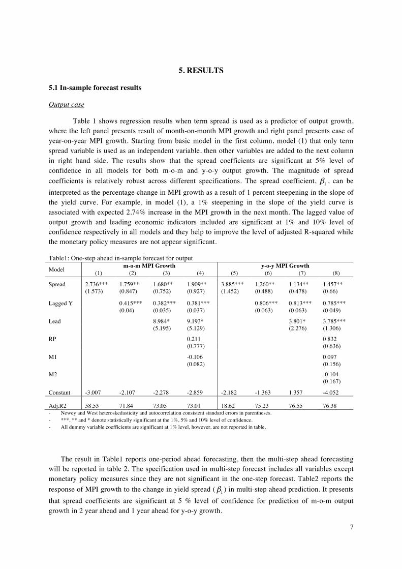
Table 1 shows regression results when term spread is used as a predictor of output growth, where the left panel presents result of month-on-month MPI growth and right panel presents case of year-on-year MPI growth. Starting from basic model in the first column, model (1) that only term spread variable is used as an independent variable, then other variables are added to the next column in right hand side. The results show that the spread coefficients are significant at 5% level of confidence in all models for both m-o-m and y-o-y output growth. The magnitude of spread coefficients is relatively robust across different specifications. The spread coefficient, , can be interpreted as the percentage change in MPI growth as a result of 1 percent steepening in the slope of the yield curve. For example, in model (1), a 1% steepening in the slope of the yield curve is associated with expected 2.74% increase in the MPI growth in the next month. The lagged value of output growth and leading economic indicators included are significant at 1% and 10% level of confidence respectively in all models and they help to improve the level of adjusted R-squared while the monetary policy measures are not appear significant.
Table1: One-step ahead in-sample forecast for output Model m-o-m MPI Growth y-o-y MPI Growth
(1) (2) (3) (4) (5) (6) (7) (8)
Spread 2.736*** 1.759** 1.680** 1.909** 3.885*** 1.260** 1.134** 1.457** (1.573) (0.847) (0.752) (0.927) (1.452) (0.488) (0.478) (0.66)
Lagged Y 0.415*** 0.382*** 0.381*** 0.806*** 0.813*** 0.785*** (0.04) (0.035) (0.037) (0.063) (0.063) (0.049)
Lead 8.984* 9.193* 3.801* 3.785*** (5.195) (5.129) (2.276) (1.306)
RP 0.211 0.832 (0.777) (0.636)
M1 -0.106 0.097 (0.082) (0.156)
M2 -0.104 (0.167)
Constant -3.007 -2.107 -2.278 -2.859 -2.182 -1.363 1.357 -4.052
Adj.R2 58.53 71.84 73.05 73.01 18.62 75.23 76.55 76.38 - Newey and West heteroskedasticity and autocorrelation consistent standard errors in parentheses. - ***, ** and * denote statistically significant at the 1%, 5% and 10% level of confidence. - All dummy variable coefficients are significant at 1% level, however, are not reported in table.
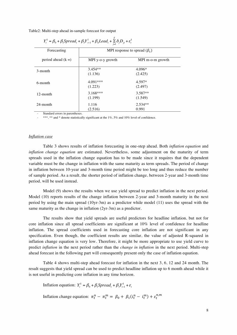
The result in Table1 reports one-period ahead forecasting, then the multi-step ahead forecasting will be reported in table 2. The specification used in multi-step forecast includes all variables except monetary policy measures since they are not significant in the one-step forecast. Table2 reports the response of MPI growth to the change in yield spread ( ) in multi-step ahead prediction. It presents that spread coefficients are significant at 5 % level of confidence for prediction of m-o-m output growth in 2 year ahead and 1 year ahead for y-o-y growth.
β1
β1
8
Table2: Multi-step ahead in-sample forecast for output
Forecasting
period ahead (k =)
MPI response to spread (𝛽!)
MPI y-o-y growth MPI m-o-m growth
3-month 3.454** (1.136)
4.096* (2.425)
6-month 4.091*** (1.223)
4.597* (2.497)
12-month 3.168*** (1.199)
3.587** (1.549)
24-month 1.116 (2.516)
2.534** 0.991
- Standard errors in parentheses. - ***, ** and * denote statistically significant at the 1%, 5% and 10% level of confidence.
Inflation case
Table 3 shows results of inflation forecasting in one-step ahead. Both inflation equation and inflation change equation are estimated. Nevertheless, some adjustment on the maturity of term spreads used in the inflation change equation has to be made since it requires that the dependent variable must be the change in inflation with the same maturity as term spreads. The period of change in inflation between 10-year and 3-month time period might be too long and thus reduce the number of sample period. As a result, the shorter period of inflation change, between 2-year and 3-month time period, will be used instead.
Model (9) shows the results when we use yield spread to predict inflation in the next period. Model (10) reports results of the change inflation between 2-year and 3-month maturity in the next period by using the main spread (10yr-3m) as a predictor while model (11) uses the spread with the same maturity as the change in inflation (2yr-3m) as a predictor.
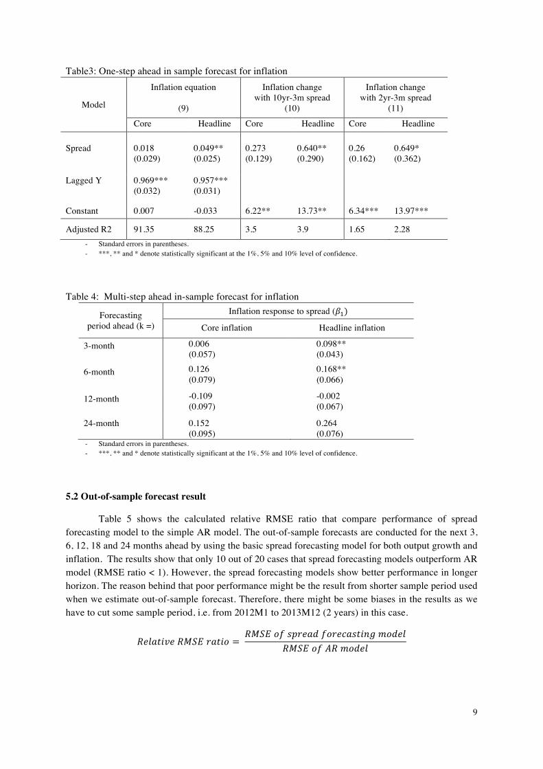
The results show that yield spreads are useful predictors for headline inflation, but not for core inflation since all spread coefficients are significant at 10% level of confidence for headline inflation. The spread coefficients used in forecasting core inflation are not significant in any specification. Even though, the coefficient results are similar, the value of adjusted R-squared in inflation change equation is very low. Therefore, it might be more appropriate to use yield curve to predict inflation in the next period rather than the change in inflation in the next period. Multi-step ahead forecast in the following part will consequently present only the case of inflation equation.
Table 4 shows multi-step ahead forecast for inflation in the next 3, 6, 12 and 24 month. The result suggests that yield spread can be used to predict headline inflation up to 6 month ahead while it is not useful in predicting core inflation in any time horizon.
Inflation equation: Ytk = β0 +β1Spreadt +β3Yt−1
k +εt
Inflation change equation: 𝜋!! − 𝜋!! = 𝛽! + 𝛽! 𝑖!! − 𝑖!! + 𝜀!!,!
Ytk = β0 +β1Spreadt +β3Y
1t−1 +β4Leadt + Σj=1
dδ jDjt +εt
k
9
Table3: One-step ahead in sample forecast for inflation
Model
Inflation equation
(9)
Inflation change with 10yr-3m spread
(10)
Inflation change with 2yr-3m spread
(11)
Core Headline Core Headline Core Headline Spread
0.018
0.049**
0.273
0.640**
0.26
0.649*
(0.029) (0.025) (0.129) (0.290) (0.162) (0.362)
Lagged Y 0.969*** 0.957*** (0.032) (0.031)
Constant 0.007 -0.033 6.22** 13.73** 6.34*** 13.97***
Adjusted R2 91.35 88.25 3.5 3.9 1.65 2.28 - Standard errors in parentheses. - ***, ** and * denote statistically significant at the 1%, 5% and 10% level of confidence.
Table 4: Multi-step ahead in-sample forecast for inflation
Forecasting period ahead (k =)
Inflation response to spread (𝛽!)
Core inflation Headline inflation
3-month 0.006 (0.057)
0.098** (0.043)
6-month 0.126 (0.079)
0.168** (0.066)
12-month -0.109 (0.097)
-0.002 (0.067)
24-month 0.152 (0.095)
0.264 (0.076)
- Standard errors in parentheses. - ***, ** and * denote statistically significant at the 1%, 5% and 10% level of confidence.
5.2 Out-of-sample forecast result
Table 5 shows the calculated relative RMSE ratio that compare performance of spread forecasting model to the simple AR model. The out-of-sample forecasts are conducted for the next 3, 6, 12, 18 and 24 months ahead by using the basic spread forecasting model for both output growth and inflation. The results show that only 10 out of 20 cases that spread forecasting models outperform AR model (RMSE ratio < 1). However, the spread forecasting models show better performance in longer horizon. The reason behind that poor performance might be the result from shorter sample period used when we estimate out-of-sample forecast. Therefore, there might be some biases in the results as we have to cut some sample period, i.e. from 2012M1 to 2013M12 (2 years) in this case.
𝑅𝑒𝑙𝑎𝑡𝑖𝑣𝑒 𝑅𝑀𝑆𝐸 𝑟𝑎𝑡𝑖𝑜 = 𝑅𝑀𝑆𝐸 𝑜𝑓 𝑠𝑝𝑟𝑒𝑎𝑑 𝑓𝑜𝑟𝑒𝑐𝑎𝑠𝑡𝑖𝑛𝑔 𝑚𝑜𝑑𝑒𝑙
𝑅𝑀𝑆𝐸 𝑜𝑓 𝐴𝑅 𝑚𝑜𝑑𝑒𝑙
10
Table 5 Out-of-sample forecast result - Relative RMSE ratio
Horizon Output growth Inflation
y-o-y m-o-m Core Headline
3-Month 0.926 2.797 1.100 3.057
6-Month 0.914 1.014 0.962 0.430
12-Month 1.010 1.003 0.922 1.513
18-Month 1.005 0.985 0.928 1.602
24-Month 1.004 0.975 0.942 0.921
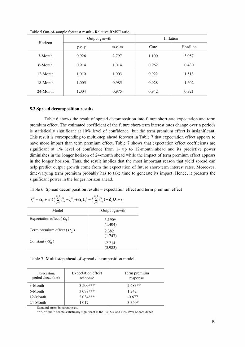
5.3 Spread decomposition results
Table 6 shows the result of spread decomposition into future short-rate expectation and term premium effect. The estimated coefficient of the future short-term interest rates change over n periods is statistically significant at 10% level of confidence but the term premium effect is insignificant. This result is corresponding to multi-step ahead forecast in Table 7 that expectation effect appears to have more impact than term premium effect. Table 7 shows that expectation effect coefficients are significant at 1% level of confidence from 1- up to 12-month ahead and its predictive power diminishes in the longer horizon of 24-month ahead while the impact of term premium effect appears in the longer horizon. Thus, the result implies that the most important reason that yield spread can help predict output growth come from the expectation of future short-term interest rates. Moreover, time-varying term premium probably has to take time to generate its impact. Hence, it presents the significant power in the longer horizon ahead.
Table 6: Spread decomposition results – expectation effect and term premium effect
Model Output growth
Expectation effect (α1 ) 3.190* (1.404) Term premium effect (α2 ) 2.382 (1.747) Constant (α0 ) -2.214 (3.983)
Table 7: Multi-step ahead of spread decomposition model
Forecasting period ahead (k =)
Expectation effect response
Term premium response
3-Month 3.500*** 2.683** 6-Month 3.098*** 1.242 12-Month 2.034*** -0.677 24-Month 1.017 3.350* - Standard errors in parentheses. - ***, ** and * denote statistically significant at the 1%, 5% and 10% level of confidence
Ytk =α0 +α1( 1n Σj=0
n−1it+ jm − it
m )+α2 (itn − 1
n Σj=0
n−1it+ jm )+δoDt +εt
11
6. LIMITATION
Different maturities of term structure
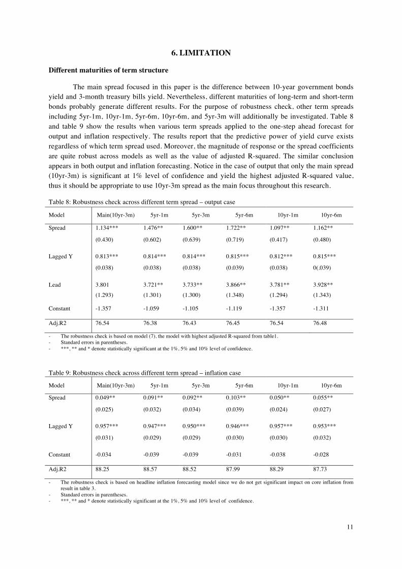
The main spread focused in this paper is the difference between 10-year government bonds yield and 3-month treasury bills yield. Nevertheless, different maturities of long-term and short-term bonds probably generate different results. For the purpose of robustness check, other term spreads including 5yr-1m, 10yr-1m, 5yr-6m, 10yr-6m, and 5yr-3m will additionally be investigated. Table 8 and table 9 show the results when various term spreads applied to the one-step ahead forecast for output and inflation respectively. The results report that the predictive power of yield curve exists regardless of which term spread used. Moreover, the magnitude of response or the spread coefficients are quite robust across models as well as the value of adjusted R-squared. The similar conclusion appears in both output and inflation forecasting. Notice in the case of output that only the main spread (10yr-3m) is significant at 1% level of confidence and yield the highest adjusted R-squared value, thus it should be appropriate to use 10yr-3m spread as the main focus throughout this research.
Table 8: Robustness check across different term spread – output case
Model Main(10yr-3m) 5yr-1m 5yr-3m 5yr-6m 10yr-1m 10yr-6m
Spread 1.134*** 1.476** 1.600** 1.722** 1.097** 1.162**
(0.430) (0.602) (0.639) (0.719) (0.417) (0.480)
Lagged Y 0.813*** 0.814*** 0.814*** 0.815*** 0.812*** 0.815***
(0.038) (0.038) (0.038) (0.039) (0.038) 0(.039)
Lead 3.801 3.721** 3.733** 3.866** 3.781** 3.928**
(1.293) (1.301) (1.300) (1.348) (1.294) (1.343)
Constant -1.357 -1.059 -1.105 -1.119 -1.357 -1.311
Adj.R2 76.54 76.38 76.43 76.45 76.54 76.48
- The robustness check is based on model (7), the model with highest adjusted R-squared from table1. - Standard errors in parentheses. - ***, ** and * denote statistically significant at the 1%, 5% and 10% level of confidence. Table 9: Robustness check across different term spread – inflation case
Model Main(10yr-3m) 5yr-1m 5yr-3m 5yr-6m 10yr-1m 10yr-6m
Spread 0.049** 0.091** 0.092** 0.103** 0.050** 0.055**
(0.025) (0.032) (0.034) (0.039) (0.024) (0.027)
Lagged Y 0.957*** 0.947*** 0.950*** 0.946*** 0.957*** 0.953***
(0.031) (0.029) (0.029) (0.030) (0.030) (0.032)
Constant -0.034 -0.039 -0.039 -0.031 -0.038 -0.028
Adj.R2 88.25 88.57 88.52 87.99 88.29 87.73
- The robustness check is based on headline inflation forecasting model since we do not get significant impact on core inflation from result in table 3.
- Standard errors in parentheses. - ***, ** and * denote statistically significant at the 1%, 5% and 10% level of confidence.

12
Difference across types of security
Rather than applying long-term government and short-term treasury bills to represent long-term and short-term interest rates, other types of securities potentially be used to represent the term spread as well. Therefore, corporate bonds and other debt securities should also be examined to see the effect across the yields. In addition, some studies argued that yield spread in large countries such US and European countries can help predicts macroeconomic variables in emerging countries. Hence, the yield spreads from those large economies might be able to apply to Thailand case as well.
Specifications of forecasting model
This paper studies the predictive content of yield curve by applying linear regression model. However, other econometric specifications could be more appropriate to examine its forecasting power. Estrella and Hardouvellis (1991), Dotsey (1998), Estrella and Mishkin (1998), Wright(2006) used probit model to study the usefulness of the term spread for predicting recessions. Abdymomunov (2009) modified Diebold-Li(2006) dynamic yield curve model based on Nelson-Seigel (1987) three latent factor framework to study the predictive ability using the entire yield curve rather than limiting information to specific maturities of spread. Furthermore, some researches used nonlinear regression models such as Dotsey (1998), Galbraith and Tkacz (2000), Duarte, Venetis, and Paya (2005). Consequently, it is possible to draw more appropriate conclusion from further study on this topic rather than the linear regression model.
Limitation of sample period and maturity of bonds
Data of short-term treasury bills yield in Thailand is available from 2001. Thus, we have limitation in sample period only from 2001 to 2014. This limitation probably generates bias in the estimation especially when we perform out-of-sample forecast that we have to cut some sample from the whole period. It is possible that the less number of sample period would not provide the best result and probably be the reason that we do not see significant improvement by applying spread forecasting model to out-of-sample forecast. In addition, the period of long-term interest rate used, which is 10-year government bonds yield, might be too long to examine its impact. Also, 10-year maturity bonds might not be actively traded in Thai bond market and hence be hardly practical for Thailand case.
7. CONCLUSION
This paper studies the ability of yield curve in predicting output and inflation for the case of Thailand. The study applies slope of the yield curve as an exogenous variable in linear regression model. The forecasts are performed for the next one to multi horizon ahead to see the predictive power over time. Both in-sample and out-of-sample forecast results show that yield spread is a useful predictor for output growth for 1 up to 12 months ahead. In case of inflation, its predictive content for headline inflation appears up to 6 month ahead. However, out-of-sample outcomes suggest that spread forecasting models do not significantly outperform AR model performance. The possible reason behind that poor performance is the relatively short period of availability of data in Thailand,
13
particularly a small number of sample period left when we estimate out-of-sample models. In the decomposition of term spread on the basis of expectation hypothesis, the results show that the contribution of the future expected change of short- term rates to prediction of real economic activity is significantly greater than that of the term premium. However, the effect of term premium appears to be more significant in longer horizon.
The empirical results show that yield curve can be used as one of a reasonable predictor for macroeconomics variables in Thailand. It will be useful implication for policymaker to relate the meaning of this financial indicator to the real activity. However, some improvement is required in order to derive the most appropriate model to apply in forecasting real economic activity. Further study and improvement on this topic would potentially generate a beneficial indicator for Thai economy in the future.
REFERENCE
Abdymomunov, Azamat (2009), “Predicting output and inflation using the entire yield curve.” Journal of Macroeconomics, No.37, pp.333-44.
Ang, Andrew; Piazzesi, Monika and Wei, Min (2006), "What does the yield curve tell us about GDP growth?."Journal of Econometrics, Elsevier, 131(1-2), pp. 359- 403.
Barnett, Nicholas (2012), “Learning From History: Examining Yield Spreads as a Predictor of Real Economic Activity.” Michigan Journal of Business, 5(1), January 2012, p.11.
Chen, Ming H; Wang, Kai L. and Yen, Meng F. (2005), “The Predictive Power of the Term Structures of Interest Rates: Evidences for the Developed and Asian Emerging Markets.”
Chin, Menzie D. and Kucko, Kavan J. (2010), “The Predictive power of the yield curve across countries and time.” Working Paper of National Bureau of Econmic Research, 16398, September 2010.
Dotsey, Michael (1998). “The Predictive Content of the Interest Rate Yield Spread for Future Economic Growth.” Federal Reserve Bank of Richmond Economic Quarterly, Summer 1998, 84(3), pp. 31-51
Duarte, Augustin; Venetis, Ioannis A. and Paya, Ivan (2005). “Predicting Real Growth and the Probability of Recession in the Euro Area Using the Yield Spread.” International Journal of Forecasting, April/June 2005, 21(2), pp. 262-77.
Estrella, Arturo (2005), “The yield curve as a leading indicator: Frequently asked questions.” Current issues in Economics and Finance.
Estrella, Arturo, and Frederic S. Mishkin (1998), "Predicting U.S. Recessions: Financial Variables as
Leading Indicators." Review of Economics and Statistics, 80(1), pp.45-61.

14
Estrella, Arturo and Hardouvelis, G. (1991), “The term structure of interest rates and its role in monetary policy for the European Central Bank.” European Economic Review, vol. 41, pp. 1375-401.
Estrella, Arturo and Mishkin, Frederic S. (1997), “The Predictive Power of the Term Structure of
Interest Rates in Europe and the United States: Implications for the European Central Bank.” European Economic Review, 41(7) ,July 1997, pp. 1375-401.
Estrella, Arturo; Rodrigues, Anthony P. and Schich, Sebastian (2003), “How Stable Is the Predictive Power of the Yield Curve? Evidence from Germany and the United States.” Review of Economics and Statistics, 85(3), August 2003, pp. 629-44.
Estrella, Arturo and Trubin, Mary R. (2006), “The Yield Curve as a Leading Indicator: Some Practical Issues.” Current issues in economics and finance, 12(5),July/August 2006.
Hamilton, James D. and Kim, Dong H. (2002), “A Re-Examination of the Predictability of the Yield Spread for Real Economic Activity.” Journal of Money, Credit, and Banking, 34(2), May 2002,pp. 340-60.
Haubrich, Joseph G. and Dombrosky, Ann M. (1996), “Predicting real growth using the yield curve.” Federal Reserve Bank of Cleveland, Economic review, 32(1), pp.26-35.
Jorion, Philippe, and Frederic Mishkin (1991), " A Multicountry Comparison of Term-structure Forecasts at Long Horizons." Journal of Financial Economics, 29(1), pp. 59-80.
Lowe, Phillip (1992), “The term structure of interest rates, real activity and inflation.” Research Discussion Paper, No. 9204, May 1992.
Mehl, A. (2006), “The yield curve as a predictor and emerging economies.” Working paper series of European Central Bank, No. 691, November 2006.
Mishkin, Frederic (1990), “What Does the Term Structure Tell Us about Future Inflation?” Journal of Monetary Economics, 25, pp. 77-95.
Smets, Frank and Tsatsaronis, Kostas (1997), “Why does the yield curve predict economic activity?: Dissecting the evidence for Germany and the United States.” Working papers of Bank for International Settlements, No.49, September 1997.
Stock, James H. and Watson, Mark W. (2003), “Forecasting Output and Inflation: The Role of Asset Prices.” Journal of Economic Literature, 41(3), September 2003, pp. 788-829.
Thornton, Daniel L. (2004), “.” Federal Reserve Bank of St. Louis Review, 86(5), September/October 2004, pp. 21-39.
Tkacz, Greg (2001). “Neural Network Forecasting of Canadian GDP Growth.” International Journal of Forecasting, January/March 2001, 17(1), pp. 57-69.
Wheelock, David C. and Wohar, Mark E. (2009), “Can the Term Spread Predict Output Growth and Recessions? A Survey of the Literature.” Federal Reserve Bank of St. Louis Review, 91(5, Part 1), September/October 2009, pp. 419-40.
Wright, Jonathan, H (2006). “The Yield Curve and Predicting Recessions.” Finance and Economics Discussion Series No. 2006-07, Federal Reserve Board of Governors, February 2006.
15
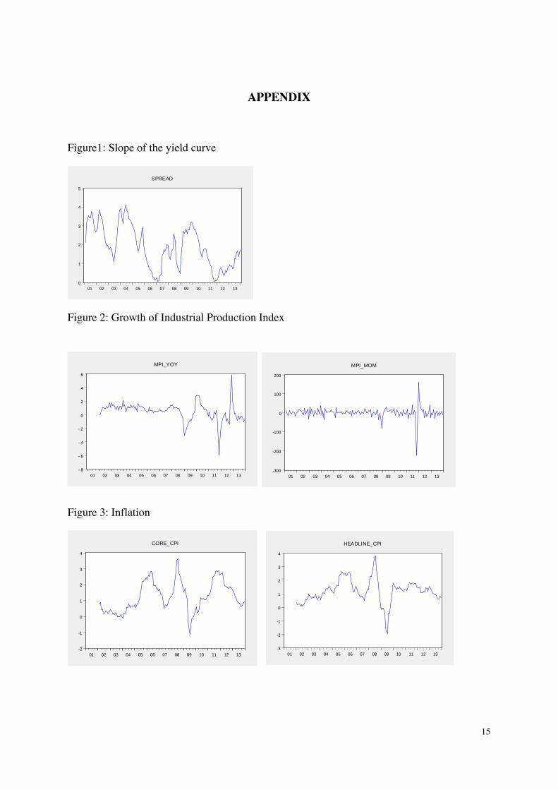
APPENDIX
Figure1: Slope of the yield curve
Figure 2: Growth of Industrial Production Index
Figure 3: Inflation
0
1
2
3
4
5
01 02 03 04 05 06 07 08 09 10 11 12 13
SPREAD
-2
-1
0
1
2
3
4
01 02 03 04 05 06 07 08 09 10 11 12 13
CORE_CPI
-3
-2
-1
0
1
2
3
4
01 02 03 04 05 06 07 08 09 10 11 12 13
HEADLINE_CPI
-.8
-.6
-.4
-.2
.0
.2
.4
.6
01 02 03 04 05 06 07 08 09 10 11 12 13
MPI_YOY
-300
-200
-100
0
100
200
01 02 03 04 05 06 07 08 09 10 11 12 13
MPI_MOM

16
Table A: Test for stationary of variables Augmented Dickey-Fuller Unit Root Test Null hypothesis: The variable has a unit root
Variable t-Statistic
Level 1st difference
Yield spread -2.937** -8.426***
Y-o-y MPI growth -2.867* -5.307***
M-o-m MPI growth -11.208*** -9.208***
Core inflation -2.470 -8.565***
Headline inflation -3.729*** -8.338*** ***, ** and * denote statistically significant at the 1%, 5% and 10% level of confidence.