The Prediction of Conveyor Trajectories - IMHC and … 02.pdf · THE PREDICTION OF CONVEYOR TRAJECTORIES ... belt conveyors are widely used as ... Accurately determining the material

Copyright vested in IMHC 1

THE PREDICTION OF CONVEYOR TRAJECTORIES DB Hastie and PW Wypych

1 INTRODUCTION From transportation of bulk materials in underground and open-cut mines to applications in power stations and processing plants to name but a few, belt conveyors are widely used as an economical continuous conveying method. Most of these industries rely strongly on conveyor transfers to divert material from one conveyor to another at some point in their system. The unfortunate reality is that some companies will be driven by cost minimisation for the short-term rather than planning for the long-term. This will result in bad decisions being made and the incorrect conveyor transfer being installed with flow-on effects such as downtime for modifications or even replacement. There are many facets to the design of a successful transfer chute including minimising product impact, degradation, chute wear, noise, dust and spillage while maximising the material velocity to allow the product to leave the chute at or near the speed of the receiving conveyor. Fully understanding the behaviour of a material is paramount to designing a successful transfer chute. Accurately determining the material discharge and trajectory from the head pulley is the first step in this design process. This paper will focus on the determination of the material trajectory as it leaves the belt conveyor head pulley. This process will also determine the point at which the material leaves the belt, referred to as the discharge angle. There are numerous methods available in the literature focusing on the modelling of material discharge and trajectory, including C.E.M.A. [1, 2, 3, 4, 5], M.H.E.A. [6, 7], Booth [8], Golka [9, 10], Korzen [11], Goodyear [12] and Dunlop [13]. These methods have been evaluated for both horizontal and inclined belts for a range of belt speeds and pulley diameters to evaluate both low and high-speed conditions. The results of these evaluations have been compared to allow comment on their ease of use, completeness and potential accuracy. 2 TRAJECTORY METHODS EXAMINED 2.1 Discharge Angles Within each of the methods presented, the discharge angle of material leaving the head pulley is determined analytically or graphically which then dictates the starting position of the material trajectory. As will be evident in section 3, it was found that there are numerous approaches to determine this discharge angle with some methods comparable to each other while some being vastly different. The resulting trajectories generated will vary significantly, also detailed in section 3. Of course there should only be one discharge angle for a given material and set of conditions. 2.2 Horizontal and Inclined Conveyor Geometries The Conveyor Equipment Manufacturers Association has released six editions of the C.E.M.A. guide, ‘Belt Conveyors for Bulk Materials’ since 1966. The first five editions follow the same procedure for determination of material trajectory with only slight adjustments to various values in reference tables. In the 6th Edition of the C.E.M.A. guide [5], there is a change to how the time interval is calculated for high-speed belts for determining the trajectory profile, now being calculated based on the belt speed rather than the tangential velocity. For all other conditions, the time intervals are calculated as per the previous editions. The C.E.M.A. method addresses seven conveyor conditions:

- low-speed belts where material wraps around the pulley before discharge (horizontal, inclined and declined belts),

- high-speed belts where material discharges at the point of tangency between the belt and head pulley (horizontal, inclined and declined belts), and

- inclined belts where material discharges at the top most vertical point of contact between the belt and the pulley (inclined belts).


The equations presented in Table 1 represent the conditions, which need to be satisfied to determine which of the seven cases above is to be used. If low-speed conditions exist,

equation (7) is used to determine the discharge angle, d.

Low-speed Medium High-speed

Horizontal

2

1s

c

V

gR (1) N/A

2

1s

c

V

gR (2)

Inclined

2

cossb

c

V

gR (3)

2

1s

c

V

gR (4)

2

1s

c

V

gR (5)

2

cos 1sb

c

V

gR (6)

Table 1 Belt speed conditions for the C.E.M.A. [1, 2, 3, 4, 5] and M.H.E.A. [7] methods

2

cos

sd

c

V

g R (7)

The trajectory produced by the C.E.M.A. method is based on the centroidal path. To plot the trajectory, a tangent line is drawn from the point at which the material leaves the pulley. At regular time intervals along this tangent line, vertical lines are projected down to fall distances supplied in the C.E.M.A. guide. A curve is then drawn through these points to produce the centroid trajectory. The upper and lower trajectory limits can also be plotted by offsetting from the centroidal curve the distance to the belt and to the load height. It is evident from this procedure that a constant width trajectory path results. C.E.M.A. notes that for light fluffy materials, a high belt speed will alter the upper and lower limits with both vertical and lateral spread due to air resistance. The Mechanical Handling Engineer’s Association guide, ‘Recommended Practice for Troughed Belt Conveyors’ [6] addresses both low-speed and high-speed belts via centripetal acceleration. The speed conditions of Table 1 are used, this time using pulley diameter rather than material centroid, resulting in the determination of the lower trajectory. This method [6] also provides an approximation for the outer trajectory of the material by first determining the

angle, d2, at which the upper surface of material starts its trajectory. The M.H.E.A. released a second edition of the guide [7], which better explains the method of determining the material trajectory. On inspection, it is identical to the C.E.M.A. method up to and including the 5th Edition. However, it uses metric rather than imperial units and the conversion results in minor differences, ultimately causing minor variations to the trajectory curves, which are, determined exactly the same as for the C.E.M.A. method. Booth [8] found that while using available theory, a large discrepancy was present between the theory and that of the actual trajectory. After careful investigation and confirmation of these errors, Booth concluded that, for one, the effects of the material slip were not being addressed as material discharged over the head pulley. This led to an analytical analysis to develop a more representative theory.

Booth’s method begins by determining the angle, , at which the particle will leave the head pulley, again based on the low-speed and high-speed conditions described by the C.E.M.A. method [1, 2, 3, 4, 5]. For low-speed conditions, an initial estimate of the discharge angle is found using equation

(8), followed by the angle at which material slip first occurs on the belt, r, equation (9). The

analytical analysis by Booth produces equation (10) and by setting bVV and r


the constant of integration, C, can be determined. Once C has been defined, equations (8)

and (10) are solved simultaneously using dV V and d to determine the

discharge angle and discharge velocity.

2

cos bd

b

V

gR (8)

21

cos sinbr r

b

V

gR

(9)

22

2

2

2 1 cos 3 sin

2 4 1b

VC e

g R

(10)

The trajectory is then plotted calculating a time interval from the tangent line and projecting down the freefall distances provided by Booth. However, there is no mention of how the upper trajectory is determined or how the material height at the discharge point is calculated. Booth acknowledged that this method was tedious and complicated and as an alternative, developed a chart to minimise the time required to analyse a particular belt conveyor geometry still with a reasonable accuracy. Golka’s method [9, 10] for determining material trajectory is based on the Cartesian coordinate system and is for materials without cohesion or adhesion. For low-speed belts, this method once again follows that of C.E.M.A. in determining the discharge angle of the lower trajectory using equation (2). It also calculates a separate discharge angle for the upper trajectory by substituting the radius of the upper trajectory into equation (2). The material height on the belt before discharge is taken directly from C.E.M.A. however, an adjusted material height, hd, is also calculated for the point at which the upper trajectory discharges from the pulley, equation (11).

0.5

2 1 1d p

p

hh R

R

(11)

Two divergent coefficients have been introduced by Golka [9, 10], 1 for the lower and 2 for the upper trajectory, which takes into account variables such as air resistance, size distribution, permeability and particle segregation. Unfortunately no explanation is given as to how they are determined. A set of curves has been produced using the parameters utilised in section 3 and varying the divergent coefficients, as can be seen in Figure 1. Not knowing with any certainty what divergent coefficients should be used for a given product/condition can result in a substantial variation of the predicted trajectory curves.


-4000

-3500

-3000

-2500

-2000

-1500

-1000

-500

0

500

-500 0 500 1000 1500 2000 2500 3000 3500 4000

1 0, 2 0

1 0.1, 2 0.1

1 0.2, 2 0.2

1 0.3, 2 0.3

1 0.4, 2 0.4

DIMENSIONS IN

MILLIMETERS

Figure 1 Variation in trajectories based on different divergent coefficients

Golka [9, 10] uses three cases, Table 2, to predict the material trajectory from the pulley depending on predefined conditions. The critical velocity, Vcr, needs to be determined from equation (12) where the radius represents either the lower or the upper trajectory. This determines the velocity at which the transition from low-speed to high-speed occurs. V1 = Vb and V2 is determined from equation (13).

Condition d1 d2

CASE 1 1 1 2 2 and cr crV V V V Use equation (14) Use equation (15)

CASE 2 1 1crV V Point of tangency Point of tangency

CASE 3 1 1 2 2 and cr crV V V V Use equation (14) Point of tangency

Table 2 Discharge angle determination for the Golka method [9, 10]

coscr bV gR (12)

5.0

12

21

pR

hVV (13)

2

11cos

d

p

V

g R (14)

2

22cos

d

p d

V

g R h

(15)


The trajectory is then determined from a series of Cartesian coordinate based equations for pre-selected time steps. Golka [9, 10] does not include belt thickness when determining the radii of the lower and upper stream. Material height is included, though based on values taken from the early C.E.M.A. guide [1, 2]. Of all the methods reviewed, Korzen [11] is the most complex in its approach, addressing the issues of adhesive materials; inertia, slip and air drag in its calculations. There is also a

distinction between static friction, s, and kinematic friction, k, used in the determination of

the discharge velocity, Vd, and discharge angle, d.

For high-speed belts, d = b and Vd = Vb. For low-speed belts, the angle at which material

begins to slip on the belt before discharge, r, is determined from equation (16). To evaluate

the constant of integration, C, the conditions bVV and r are used in equation

(17). To determine the discharge angle, the relationships cos 2 gRV c and d

are used.

2

1 1 1tan sin sin tan 2

b ar s s

c

V

R g h

(16)

2

42

2

4 1 cos 5 sin( ) 2

1 16

kk k

c

k

V gR Ce

(17)

The detailed numerical analysis developed by Korzen is achieved by a series of successive approximations, which incorporate ‘corrected’ air drag coefficients based on particle shape and a proportionality factor for air drag. Using the X-displacement for any given position of the trajectory, the Y-displacement, trajectory angle and resultant velocity can be obtained. The first approximation is for a free falling particle in a vacuum, which is used as the initial trajectory estimate, where air drag is neglected, for all other approximations, air drag is applied. The analysis is continued until the differential error between successive approximations have deviations no greater than 1% or 2%. Once the analysis has been completed for a suitable range of X-displacements, the X and Y coordinates are plotted to produce the trajectory for the central path. The discharge angle and discharge velocity calculated above are for the centre height of the material stream. Korzen [11] also allows for calculation of the upper and lower trajectory limit discharge velocities. For high-speed belts, the upper and lower discharge velocities are the same as that for the centre height trajectory but for a low-speed belt, the discharge velocities are calculated based on ratios of the radius of the lower and upper trajectories. For particles over 1g in mass, the effects of air drag can be dismissed [11]. This being the case, only the first approximation is performed and the trajectory is plotted from those values. This will also result in the trajectory curves having a closer match to those generated by other methods. Although the discharge velocity for the lower and upper trajectories can be determined, there is no method described for the determination of the corresponding trajectories. The assumption has been made that the same approximation method is used, substituting the calculated discharge velocity for the appropriate trajectory. Korzen [11] does not include the belt thickness when determining the trajectory curves. Although as a percentage of the head pulley diameter the belt thickness is quite small, this omission will result in a minor vertical offset of the plotted trajectories compared to methods, which include belt thickness. There also appears to be several errors in the worked examples presented by Korzen [11]. As a result of one group of errors, additional approximations were required to achieve an adequate error level. Also, in several quoted equations there also


appears to be some typographical errors, which can raise questions as to whether the method is being applied correctly. The ‘Handbook of Conveyor and Elevator Belting’ [12] is quite simplistic in its approach to determining material trajectory. Using the principles of projectile motion, equation (18) and equation (19) are used to determine the X and Y coordinates of the trajectory. The discharge angle is determined for low-speed belt conditions by satisfying one of the cases in Table 1, this time using the radius of the central height of the material.

bX V t (18)

2

2

g tY (19)

Goodyear [12] provides two cases for horizontal conveyor geometries, which are identical to those of equations (1) and (2). For low-speed inclined conveyors equation (3) is again used, however, for high-speed inclined conveyors equation (20) is used. The Goodyear method determines the discharge angle for the central material stream, (i.e. h/2); however, there is no reference to the determination of the discharge angles or trajectories for the lower or upper trajectories. The assumption has been made that all discharge angles are of equal value, thus resulting in parallel trajectory streams. Once the X and Y coordinates and the discharge angle have been determined, producing the trajectory curve is straightforward.

2

cossb

c

V

gR (20)

Belt thickness is not used in the Goodyear method [12] and as this method determines only the centre trajectory path, a material height must be known. The worked examples by Goodyear [12] incorporate half the material height into the radius used to determine the central trajectory path without implicitly providing details of the origin of the material height. Goodyear states that the actual trajectory may be different to that of the one calculated due to other forces acting on the particle stream which haven’t been used in these calculations. The Dunlop Conveyor Manual [13] uses a graphical method to determine the material trajectory leaving the conveyor for low-speed belts and analytical method for high-speed belts. For high-speed belts, material again leaves the belt at the point where the belt is at a tangent to the pulley. To calculate the X coordinate, the distance travelled tangentially from the belt, equation (18) is used and the Y coordinate, the distance material falls below the tangent line, is calculated using equation (19). Dunlop states that the mathematics behind the trajectory for low-speed conveyors is complex and so developed a graphical method. Knowing the belt speed and pulley diameter, it is a simple process to determine the discharge angle and X, the incremental distance along the discharge tangent line. At each of these incremental distances, Y is projected vertically down with the same values as for high-speed conveyors. If it is found that the desired belt speed does not intersect with the required pulley diameter then the method for high-speed belts should be used. For the low-speed condition, pulley diameters between 312mm and 1600mm are presented. Outside of this range, there is no way to estimate the discharge angle or X. The resulting trajectory is a prediction of the lower boundary. There is reference to material depth in the worked examples in the Dunlop Conveyor Manual but no explanation of how it is determined and there is an indication that the flow pattern is convergent. 2.3 Declined Conveyor Belts Only three methods, C.E.M.A. [1, 2, 3, 4, 5], M.H.E.A. [7] and Goodyear [12] allow for the determination of the discharge angle for declined belt conveyors and while Dunlop [13] makes no specific mention of declined conveyor belts in its guide, it alludes to a declined conveyor belt having the same discharge angle as a horizontal or inclined conveyor via a worked


example. For this reason declined conveyors have not been incorporated into the comparisons of section 3, however will briefly be discussed. Up to and including the fifth edition of the C.E.M.A. guide [1, 2, 3, 4] and M.H.E.A [7] the low-speed or high-speed conditions are determined from equation (21). High-speed discharge is again at the point of tangency and for low-speed conditions equation (3) is used, followed by equation (7).

2

cossb

c

V

gR (21)

The sixth edition of C.E.M.A. [5] has a variation to the low-speed condition, now adding the discharge angle to the belt declination angle. However, in the worked example for this specific case, the discharge angle calculated is identical to the discharge angle found in the previous five editions of the C.E.M.A. guide, which have the discharge angle determined from the vertical. So this would in actual fact indicate that the graphical representation of this case is incorrect. The Goodyear [12] method of determining the discharge angle for declined conveyor belts uses equation (20) for high-speed conditions resulting in discharge from the tangency point and for low-speed uses equation (3) and equation (7) and is plotted from the vertical as with the earlier C.E.M.A. methods and M.H.E.A. 2.4 Critical Belt Speed The critical belt speed, touched on previously, refers to the point of transition from low-speed to high-speed conditions and Table 3 summarises the five unique equations used. As previously explained Golka [9, 10] determines two distinct discharge angles and following from this there are also two critical belt speeds. The method by Korzen [11] incorporates an adhesive stress component, however when the adhesive stress equals zero, the equation is identical to that of Goodyear [12]. For the Dunlop method [13], the critical belt speed is graphically determined for the lower and upper discharge angles. There are however limitations to it’s determination due to the maximum pulley diameter charted being 1600mm.

C.E.M.A. and M.H.E.A.

2

,

cosb bb cr

c

gRV

R

(22)

Booth and Golka (lower) , cosb cr b bV gR (23)

Golka (upper) ,

21 cosb cr b b

b

hV gR

R (24)

Korzen , cos a

b cr c bV gRh

(25)

Goodyear , cosb cr c bV gR (26)

Table 3 Critical belt speeds for the trajectory methods

2.5 Effect of Transition Geometry As the conveyor belt moves through the transition zone, stresses are generated at the belt edges and can cause permanent deformation if the elastic limit is surpassed. To minimise or even overcome this, the head pulley can be raised to ½ the trough depth thus reducing the


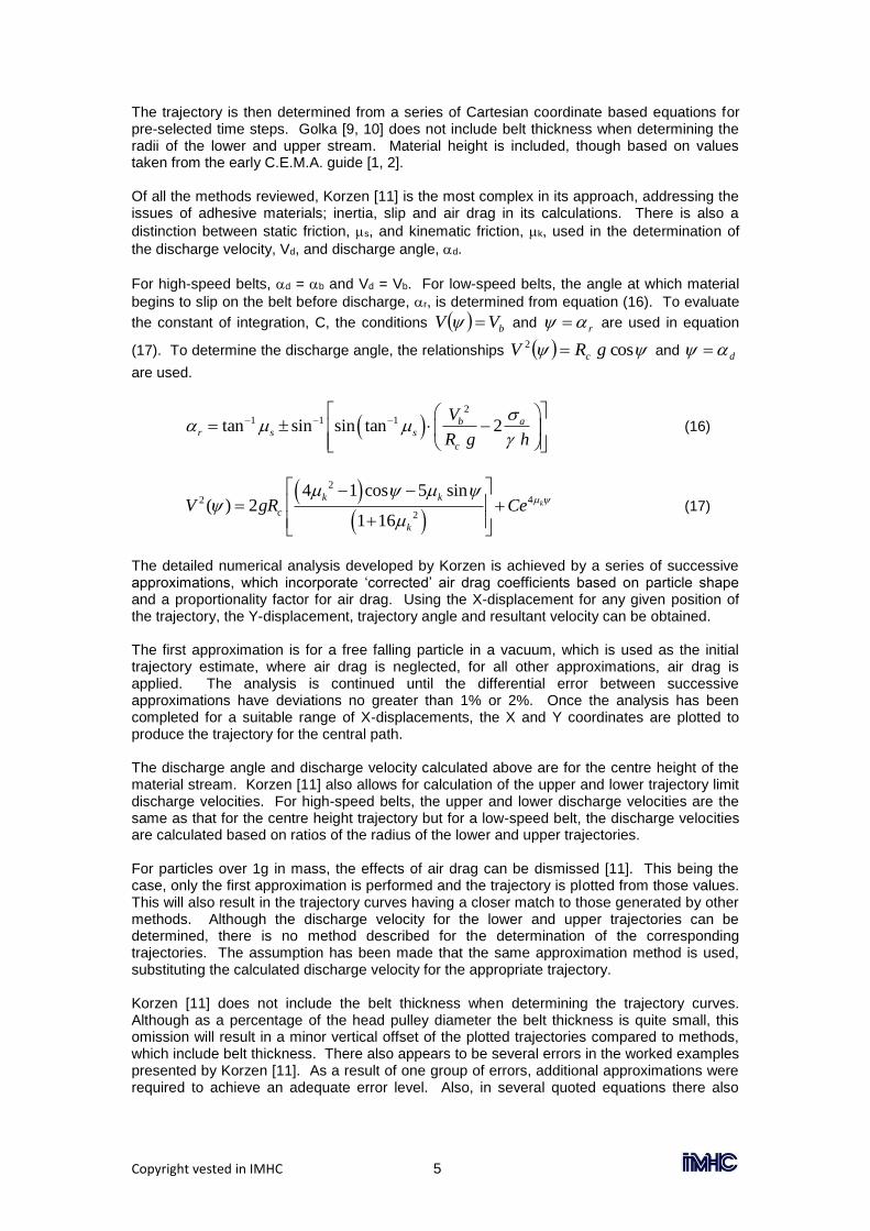
stresses on the belt [5]. Although this is stated by C.E.M.A. [5], there is no indication whether this is applied in the determination of conveyor trajectories. Roberts, Wiche et al. [14] state

that the transition angle, , does effect belt discharge trajectories and as can be seen in

Figure 2, the point of tangency of the belt to the head pulley becomes + , where is determined from equation (27).

1tan

t

z

L

(27)

For low-speed conditions, the angle 0 is determined, defining the angle that discharge

commences. For high-speed conditions discharge is at the point of tangency (i.e. 0 = 0º).

Figure 2 Transition Geometry [14] The trajectory coordinates can then be determined using equation (28).

2

0 2 2

0

tan2 cos

b

b b

gYX Y

V

(28)

The method presented by Roberts et al. [14] is the only approach which directly addresses the transition arrangement when considering the determination of the trajectory and even though a half trough transition is recommended by C.E.M.A. [5], there is no indication it is applied to the trajectory method provided. 3 TRAJECTORY METHODS COMPARED To allow for a direct comparison between all the methods described, a constant set of parameters was selected as shown in Table 4. The only variations allowed for are belt speed (Vb = 1.25, 3.0 and 6.0ms-1), pulley diameter (Dp = 0.5, 1.0 and 1.5m) and belt inclination angle (0° to 30°), all others are fixed. As adhesive stress is only accounted for by the Korzen method [11], it has been set to zero to allow comparison of all methods. Although not quantified here, if adhesive stress were to be applied, the result would be an increased discharge angle, which would result in a trajectory stream falling closer to the head pulley compared with the other methods.


PARAMETERS VALUES

Belt Width, wb 0.762 m

Belt Thickness, b 0.01 m

Belt Speed, Vb 1.25 ms-1

Pulley Diameter, Dp 0.5 m

Surcharge Angle 20 °

Troughing Angle 20 °

Belt Inclination Angle, b 0 °

Divergent Coefficient, Lower, 1 0.1 -

Divergent Coefficient, Upper, 2 -0.1 -

Coefficient of Friction, Static, s 0.5 -

Coefficient of Friction, Kinematic, k 0.42 -

Adhesion Stress, a 0 kPa

Equivalent Spherical Particle Diameter 0.001 m

Atmospheric Temperature, Tatm 20 °C

Atmospheric Pressure, Patm 101 kPa

Air Viscosity, f 1.80E-05 Nsm-2

b 2000 kgm-3

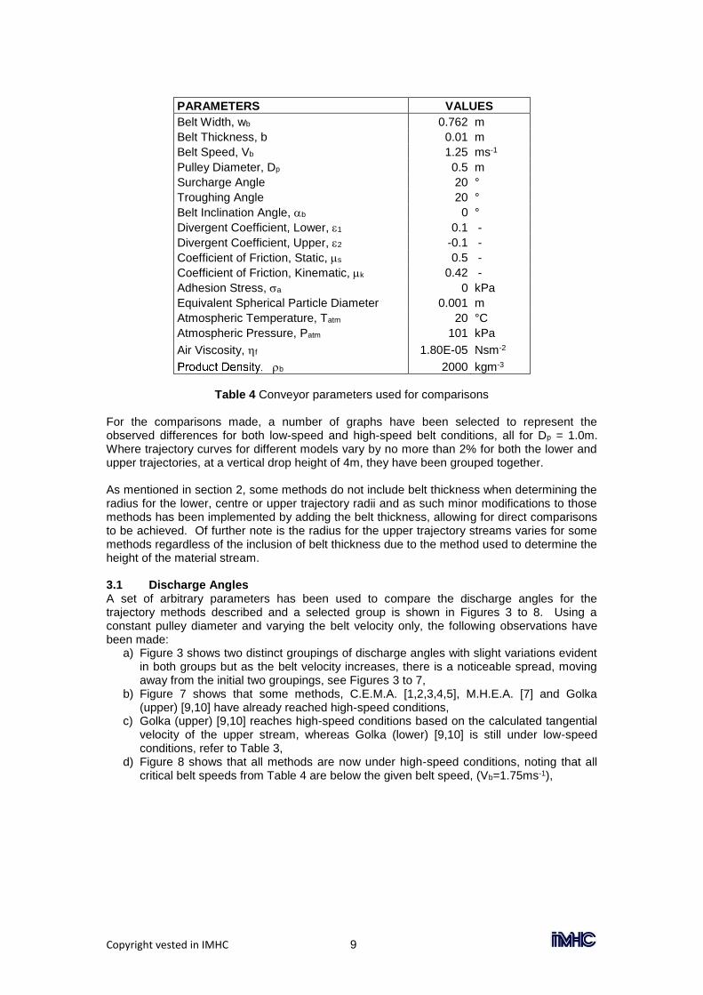
Table 4 Conveyor parameters used for comparisons

For the comparisons made, a number of graphs have been selected to represent the observed differences for both low-speed and high-speed belt conditions, all for Dp = 1.0m. Where trajectory curves for different models vary by no more than 2% for both the lower and upper trajectories, at a vertical drop height of 4m, they have been grouped together. As mentioned in section 2, some methods do not include belt thickness when determining the radius for the lower, centre or upper trajectory radii and as such minor modifications to those methods has been implemented by adding the belt thickness, allowing for direct comparisons to be achieved. Of further note is the radius for the upper trajectory streams varies for some methods regardless of the inclusion of belt thickness due to the method used to determine the height of the material stream. 3.1 Discharge Angles A set of arbitrary parameters has been used to compare the discharge angles for the trajectory methods described and a selected group is shown in Figures 3 to 8. Using a constant pulley diameter and varying the belt velocity only, the following observations have been made:

a) Figure 3 shows two distinct groupings of discharge angles with slight variations evident in both groups but as the belt velocity increases, there is a noticeable spread, moving away from the initial two groupings, see Figures 3 to 7,

b) Figure 7 shows that some methods, C.E.M.A. [1,2,3,4,5], M.H.E.A. [7] and Golka (upper) [9,10] have already reached high-speed conditions,

c) Golka (upper) [9,10] reaches high-speed conditions based on the calculated tangential velocity of the upper stream, whereas Golka (lower) [9,10] is still under low-speed conditions, refer to Table 3,

d) Figure 8 shows that all methods are now under high-speed conditions, noting that all critical belt speeds from Table 4 are below the given belt speed, (Vb=1.75ms-1),


BOOTH

GOLKA

KORZEN

CEMA 1,2,4,5

CEMA 6

MHEA86

DUNLOP

GOODYEAR

DIMENSIONS IN METRES

-0.50

-0.25

0.00

0.25

0.50

0.00 0.25 0.50 0.75

-0.50

-0.25

0.00

0.25

0.50

0.00 0.25 0.50 0.75

-0.50

-0.25

0.00

0.25

0.50

0.00 0.25 0.50 0.75

Figure 3 Dp=0.5m, Vb=0.50ms-1

Figure 4

Dp=0.5m, Vb=0.75ms-1

Figure 5

Dp=0.5m, Vb=1.00ms-1

-0.50

-0.25

0.00

0.25

0.50

0.00 0.25 0.50 0.75

-0.50

-0.25

0.00

0.25

0.50

0.00 0.25 0.50 0.75

-0.50

-0.25

0.00

0.25

0.50

0.00 0.25 0.50 0.75

Figure 6 Dp=0.5m, Vb=1.25ms-1

Figure 7

Dp=0.5m, Vb=1.50ms-1

Figure 8

Dp=0.5m, Vb=1.75ms-1

e) referring to the two discharge angles for Dunlop [13] in Figure 7, there is an indication that there is a high convergence of the lower and upper paths based on the authors’ assumption that two distinct discharge angles should be determined. There will in all likelihood be a crossing of the streams, which in reality would not occur.

Low-speed conditions are achievable over a wider range of belt speeds as the pulley diameter increases, for example, a pulley diameter of 2m will operate under low-speed conditions up to approximately 3.1ms-1. 3.2 Low-Speed Trajectories A comparison graph for the low-speed trajectory predictions is presented in Figure 9. Although having a larger pulley diameter than the example of Figure 3, Figure 9 clearly shows two main groupings of methods for the produced trajectories. It is also clear that these two groupings have an approximate horizontal variation of 500mm at a drop height of 4000mm,


which will have a marked effect on the design of a transfer chute dependant on which trajectory method is applied. Although the figures are not presented in this paper, a further trend found that as pulley diameter increases for a given belt speed, the trajectories for the models fall closer to the head pulley. The methods of Booth [8] and Dunlop [13] produce a near identical curve regardless of the fact that one uses a highly analytical approach and the other uses a straightforward graphical approach respectively.

-4000

-3500

-3000

-2500

-2000

-1500

-1000

-500

0

500

-500 0 500 1000 1500 2000 2500 3000 3500 4000

CEMA1,2,4,5,6,MHEA1986

BOOTH,DUNLOP

GOODYEAR

GOLKA,GOLKA(divergent)

KORZEN

KORZEN (air drag)

DIMENSIONS IN MILLIMETERS

Figure 9 Low-speed condition, horizontal conveyor, lower and upper trajectory path

Pulley diameter, Dp = 1.0m, belt velocity, Vb = 1.25ms-1 3.3 High-Speed Trajectories In order to investigate the change in trajectory profile due to belt speed, two high-speed belt conditions have been selected, Vb = 3.0 ms-1 and Vb = 6.0 ms-1. In Figure 10 and Figure 11, the inclusion of air drag by Korzen [11] results in a trajectory prediction clearly much shallower than all other methods. If air drag is neglected, the resulting trajectory prediction is located amongst the other methods. In section 2, it was explained that Golka [9, 10] uses divergent coefficients to obtain a better approximation of the trajectory paths. Without explanation of how these divergent coefficients have been determined, it is hard to justify using this method with any level of accuracy. If on the other hand the divergent coefficients are neglected in the calculations, the resulting trajectories are identical to the Korzen [11] method when air drag is neglected, as the equations are identical. In both cases shown, the “early” C.E.M.A. [1, 2, 3, 4] and M.H.E.A. [7] methods generate the highest trajectory curve and as the discharge velocity increases, the variation from the other curves becomes more defined. As with the low-speed conditions, the Booth [8] and Dunlop [13] methods again produce near identical trajectory curves. The incorporation of adhesive stress by Korzen [11] has been previously explained but it is clear in Figure 1 and Figure 11 that if adhesive stress were included in the calculations, the resulting trajectory curves would deviate even further from the trajectory curves of the other methods.


-4000

-3500

-3000

-2500

-2000

-1500

-1000

-500

0

500

-500 0 500 1000 1500 2000 2500 3000 3500 4000

CEMA1,2,4,5,MHEA1986

BOOTH,DUNLOP

CEMA6,GOODYEAR

GOLKA,KORZEN

GOLKA(divergent)

KORZEN (air drag)


Figure 10 High-speed condition, horizontal conveyor, lower and upper trajectory path Pulley diameter, Dp = 1.0m, belt velocity, Vb = 3.0ms-1

-4000

-3500

-3000

-2500

-2000

-1500

-1000

-500

0

500

-500 0 500 1000 1500 2000 2500 3000 3500 4000 4500 5000 5500

CEMA1,2,4,5,MHEA1986

CEMA6,BOOTH,DUNLOP,GOODYEAR,GOLKA,KORZEN

GOLKA(divergent)

KORZEN (air drag)


Figure 11 High-speed condition, horizontal conveyor, lower and upper trajectory path Pulley diameter, Dp = 1.0m, belt velocity, Vb = 6.0ms-1

4 VALIDATION 4.1 Experimental A unique conveyor transfer research facility, Figure 12, will soon be commissioned at the University of Wollongong, which will allow both trajectories and variable geometry transfer chutes to be experimentally investigated. It is the intention to generate a substantial database of trajectory information from this facility addressing as many of the parameters incorporated into the trajectory methods presented. This, it is hoped, will allow direct validation of the trajectory methods and ultimately determine which of the methods is most accurate.


Figure 12 Experimental conveyor transfer research facility at University of Wollongong 4.2 Simulation The distinct element method (DEM) is an ideal simulation tool for approaching this type of granular flow problem. There are a range of commercial packages available, which will allow trajectory profiles to be simulated. This will produce another method of comparing the trajectory methods presented to the database of experimental results. It should be highlighted however, that there is probably no option for selecting how a trajectory is determined, solely being based on the physics of the commercial DEM codes (which probably do not allow for differences in moisture, cohesion, etc). The simulations may or may not correspond to the trajectory methods presented and will be evaluated as required. 5 CONCLUSION This paper has presented a number of the more widely used and/or readily available trajectory prediction methods published in the literature. They range in complexity from the basic, Goodyear [12] and Dunlop [13], to the complex, Booth [8], Golka [9, 10] and Korzen [11]. Some methods include a multitude of parameters such as C.E.M.A. [1,2,3,4,5] and M.H.E.A. [7] while others incorporate additional parameters such as divergent coefficients [9,10] and air drag [11]. For low-speed, belt conditions there appear to be two distinct groupings of trajectory predictions, see Figure 8, when the belt speed is relatively low. However as the belt speed increases, so does the scatter of discharge angles as seen in Figure 3 to Figure 8. For high-speed belt conditions an observation made was that some of the basic methods approximated a trajectory, which was also predicted by the more complex methods, see Figure 10 and Figure 11. Incorporating air drag into the trajectory predictions [11] causes a dramatic variation from the other trajectory methods. When considering air drag, it makes sense that material will drop away much quicker than the other methods but whether it is truly representative of an actual trajectory needs to be explored further. It is fair to say that the differing approaches to determining the material trajectory result in some significant differences, which cannot all be correct. Based solely on the comparisons made in this paper, it is impossible to say with any certainty which of the methods will produce the most accurate prediction of an actual trajectory. It may even be the case that one method predicts accurately the low-speed conditions whereas another is better suited for high-speed conditions. Further research is definitely needed and with the aid of a unique conveyor transfer research facility and simulation via DEM at the University of Wollongong, this should provide a means to apply improvements to the available trajectory methods


6 ACKNOWLEDGEMENTS The authors wish to acknowledge the support of the Australian Research Council, Rio Tinto OTX and Rio Tinto Iron Ore Expansion Projects for their financial and in-kind contributions to the Linkage Project, which allows this research to be pursued. 7 NOMENCLATURE b belt thickness m C constant of integration - Dp pulley diameter m g gravity ms-2 h material depth m hd material depth at discharge m Lt transition length m Patm atmospheric pressure kPa R arbitrary radius m Rb radius to outer belt surface m Rc radius of material centroid/centre m Rp pulley radius m t increment time for trajectory path s Tatm atmospheric temperature °C V1 discharge velocity of lower boundary ms-1 V2 discharge velocity of upper boundary ms-1 Vb belt velocity ms-1 Vcr critical velocity ms-1 Vd velocity of material at discharge point ms-1 Vs tangential velocity of material at discharge point ms-1 wb belt width m z height of the transition m

initial material discharge angle measured from the vertical °

b belt inclination angle °

d material discharge angle measured from the vertical trajectory °

d1 material discharge angle measured from the vertical for lower trajectory °

d2 material discharge angle measured from the vertical for upper trajectory °

r angle at which slip begins to occur °

specific gravity of bulk solid kNm-3

transition angle °

1 divergent coefficient -

2 divergent coefficient -

f air viscosity Nsm-2

0 angle at which discharge commences °

coefficient of friction -

k coefficient of kinematic friction -

s coefficient of static friction -

a adhesion stress kPa 8. REFERENCES

8.1. C.E.M.A. Belt Conveyors for Bulk Materials. 1st Ed, Conveyor Equipment Manufacturers Association, 1966.

8.2. C.E.M.A. Belt Conveyors for Bulk Materials. 2nd Ed, Conveyor Equipment Manufacturers Association, 1979.

8.3. C.E.M.A. Belt Conveyors for Bulk Materials. 4th Ed, Conveyor Equipment Manufacturers Association, 1994.



8.6. M.H.E.A. Recommended Practice for Troughed Belt Conveyors, Mechanical Handling Engineer’s Association, 1977.


8.7. M.H.E.A. Recommended Practice for Troughed Belt Conveyors, Mechanical Handling Engineer’s Association, 1986.

8.8. Booth, E. P. O. "Trajectories from Conveyors - Method of Calculating Them Corrected". Engineering and Mining Journal, Vol. 135, No. 12, December 1934, pp. 552 - 554.

8.9. Golka, K. "Discharge Trajectories of Bulk Solids". 4th International Conference on Bulk Materials Storage, Handling and Transportation, Wollongong, NSW, Australia, 6th - 8th July, 1992, pp. 497 - 503.

8.10. Golka, K. "Prediction of the Discharge Trajectories of Bulk Materials". Bulk Solids Handling, Vol. 13, No. 4, November 1993, pp. 763 - 766.

8.11. Korzen, Z. "Mechanics of Belt Conveyor Discharge Process as Affected by Air Drag". Bulk Solids Handling, Vol. 9, No. 3, August 1989, pp. 289 - 297.

8.12. Goodyear Handbook of Conveyor & Elevator Belting: Section 11, 1975. 8.13. Dunlop Industrial Conveyor Manual, 1982. 8.14. Roberts, A. W., Wiche, S. J., Ilic, D. D. and Plint, S. R. "Flow Dynamics and

Wear Considerations in Transfer Chute Design". 8th International Conference on Bulk Materials Storage, Handling and Transportation, Wollongong, NSW, Australia, 5th - 8th July, 2004, Institution of Engineers, Australia, pp. 330 - 334.

9 AUTHORS CV Mr. David Hastie B.E. (Mechanical), M.E. (Honours) has been employed with the Centre for Bulk Solids and Particulate Technologies at the University of Wollongong, Australia since 1997. He is a Member of the Institution of Engineers Australia and a member of the Australian Society for Bulk Solids Handling. In July of 2005 he took up an Academic Research Fellow position within the Faculty of Engineering.

Key areas of interest include pneumatic conveying, rotary valve air leakage, particle segregation and conveyor transfers and trajectories and has extensive experience in experimental investigations, instrumentation, data acquisition and analysis, computer programming and digital video imaging and processing.

He was the main researcher on the successful IFPRI, Inc. funded project, 1998-2004 on the prediction of transport boundaries in fluidised dense-phase and low-velocity pneumatic conveying and currently he is Research Associate on a three year project titled ‘Quantification And Modelling Of Particle Flow Mechanisms In Conveyor Transfers’. He is also a part-time PhD candidate working on transfer chute quantification and modelling. Peter Wypych B.E. (Mechanical, Honours 1), PhD is the Director of the ARC endorsed Key Centre for Bulk Solids and Particulate Technologies at the University of Wollongong. He has been involved with the research and development of solids handling and processing technology since 1981. Peter Wypych has published over 280 articles. He is currently Chair of the Australian Society for Bulk Solids Handling.

Peter Wypych is also the General Manager of Bulk Materials Engineering Australia and has completed over 450 industrial projects, involving R&D of new technologies, feasibility studies, troubleshooting, general/concept design, optimisation, debottlenecking, safety/hazard audits and/or rationalisation of plants and processes for companies all around Australia and in the USA, Hong Kong, New Zealand, China, Singapore and Korea. 10 AUTHOR CONTACTS Mr David Hastie Centre for Bulk Solids and Particulate Technologies Faculty of Engineering, University of Wollongong Northfields Avenue, Wollongong, NSW, 2522, Australia Email: [email protected] A/Prof Peter Wypych Centre for Bulk Solids and Particulate Technologies Faculty of Engineering, University of Wollongong Northfields Avenue, Wollongong, NSW, 2522, Australia Email: [email protected]

Documents

The Prediction of Conveyor Trajectories - IMHC and … 02.pdf · THE PREDICTION OF CONVEYOR TRAJECTORIES ... belt conveyors are widely used as ... Accurately determining the material