TH

E P

OW

ER

TR

AN

SF

OR

ME

RTESTING AND COMMISIONING

DET310

CHAPTER 5

CURRENT TRANSFORMER AND VOLTAGE TRANSFORMER

TESTING AND COMMISIONING

DET310

5.1 INTRODUCTION

Current or voltage instrument transformers are necessary for isolating

the protection, control and measurement equipment from the high

voltages of a power system, and for supplying the equipment with the

appropriate values of current and voltage - generally these are 1A or

5Α for the current coils, and 120 and 240 V for the voltage coils.

-continue-

The behaviour of current and voltage transformers during and after the occurrence

of a fault is critical in electrical protection since errors in the signal from a

transformer can cause mal-operation of the relays.

In addition, factors such as the transient period and saturation must be taken into

account when selecting the appropriate transformer.

5.1 Voltage Transformers

With voltage transformers (VTs) it is essential that the voltage from the secondary

winding should be as near as possible proportional to the primary voltage.

          In order to achieve this, VTs are designed in such a way that the voltage

drops in the windings are small and the flux density in the core is well below the

saturation value so that the magnetization current is small; in this way

magnetization impedance is obtained which is practically constant over the

required voltage range. The secondary voltage of a VT is usually 110 or 120 V

with corresponding line-to-neutral values. The majority of protection relays have

nominal voltages of 110 or 63.5 V, depending on whether their connection is line-

to-line or line-to-neutral

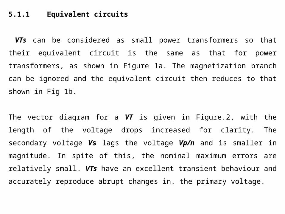
5.1.1 Equivalent circuits

VTs can be considered as small power transformers so that their equivalent circuit is

the same as that for power transformers, as shown in Figure 1a. The magnetization

branch can be ignored and the equivalent circuit then reduces to that shown in Fig

1b.

The vector diagram for a VT is given in Figure.2, with the length of the voltage drops

increased for clarity. The secondary voltage Vs lags the voltage Vp/n and is smaller

in magnitude. In spite of this, the nominal maximum errors are relatively small. VTs

have an excellent transient behaviour and accurately reproduce abrupt changes in.

the primary voltage.

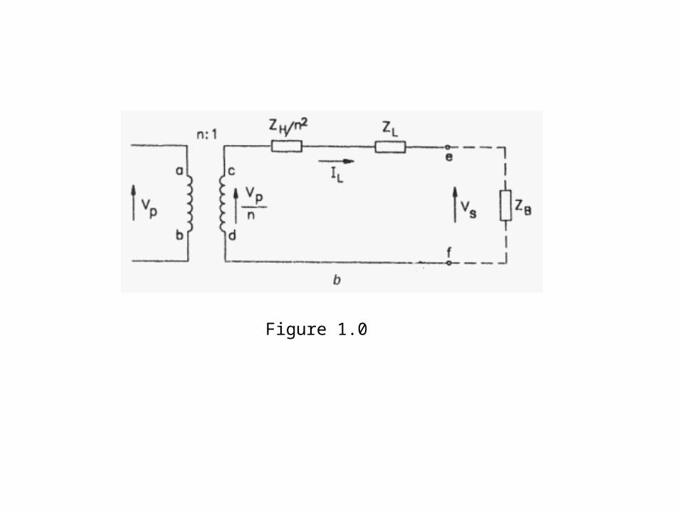
Figure 1.0

Figure 2

5.1.2 Errors

When used for measurement instruments, for example for billing and control

purposes, the accuracy of a VT is important, especially for those values close to

the nominal system voltage.

    Not withstanding this, although the precision requirements of a VT for protection

applications are not so high at nominal voltages, owing to the problems of having

to cope with a variety of different relays, secondary wiring burdens and the

uncertainty of system parameters, errors should he contained within narrow limits

over a wide range of possible voltages under fault conditions.

     This range should be between 5 and 173% of the nominal primary voltage for

VTs connected between line and earth.

  

-continue-

 Referring to the circuit in Figure 1a, errors in a VT are clue to differences in

magnitude and phase between Vp/n, and Vs. These consist of the errors under

open-circuit conditions when the load impedance ΖB is infinite, caused by the drop

in voltage from the circulation of the magnetization current through the primary

winding, and errors due to voltage drops as a result of the load current IL flowing

through both windings. Errors in magnitude can be calculated from

Error VT= {(n Vs - Vp) / Vp} x 100%

If the error is positive, then the secondary voltage exceeds the nominal value.

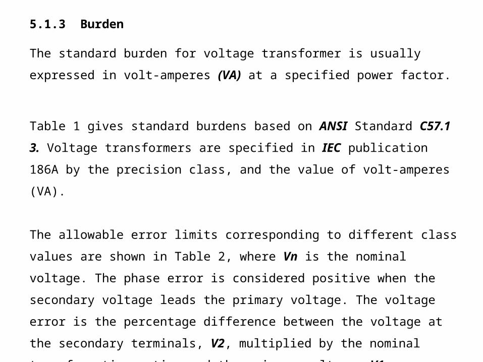
5.1.3 Burden

The standard burden for voltage transformer is usually expressed in volt-

amperes (VΑ) at a specified power factor.

Table 1 gives standard burdens based on ANSI Standard C57.1 3. Voltage

transformers are specified in IEC publication 186Α by the precision class, and

the value of volt-amperes (VΑ).

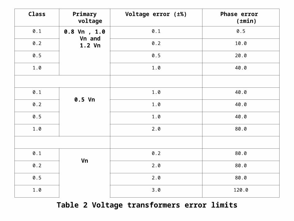
The allowable error limits corresponding to different class values are shown in

Table 2, where Vn is the nominal voltage. The phase error is considered

positive when the secondary voltage leads the primary voltage. The voltage

error is the percentage difference between the voltage at the secondary

terminals, V2, multiplied by the nominal transformation ratio, and the primary

voltages V1.

5.1.4 Selection of VT’s

Voltage transformers are connected between phases, or between phase and earth. The

connection between phase and earth is normally used with groups of three single-phase

units connected in star at substations operating with voltages at about 34.5 kV or higher,

or when it is necessary to measure the voltage and power factor of each phase

separately.

The nominal primary voltage of a VT is generally chosen with the higher nominal

insulation voltage (kV) and the nearest service voltage in mind. The nominal secondary

voltages are generally standardized at 110 and 120 V. In order to select the nominal

power of a VT, it is usual to acid together all the nominal VΑ loadings of the apparatus

connected to

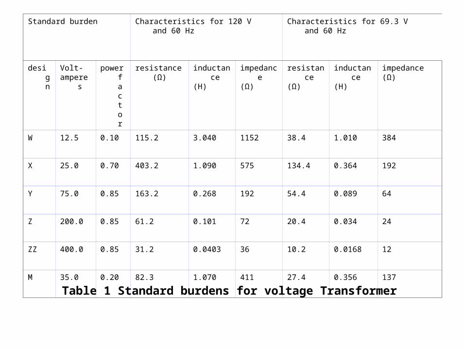
Standard burden Characteristics for 120 V and 60 Hz

Characteristics for 69.3 V and 60 Hz 

design Volt-amperes

powerfactor

resistance(Ω) inductance(H)

impedance(Ω)

resistance(Ω)

inductance(H)

impedance(Ω)

W 12.5 0.10 115.2 3.040 1152 38.4 1.010 384

Χ 25.0 0.70 403.2 1.090 575 134.4 0.364 192

Υ 75.0 0.85 163.2 0.268 192 54.4 0.089 64

Ζ 200.0 0.85 61.2 0.101 72 20.4 0.034 24

ΖΖ 400.0 0.85 31.2 0.0403 36 10.2 0.0168 12

Μ 35.0 0.20 82.3 1.070 411 27.4 0.356 137

Table 1 Standard burdens for voltage Transformer

Class Primary voltage Voltage error (±%) Phase error (±min)

0.1 0.8 Vn , 1.0 Vn and 1.2 Vn

0.1 0.5

0.2 0.2 10.0

0.5 0.5 20.0

1.0 1.0 40.0

 

0.1  0.5 Vn

1.0 40.0

0.2 1.0 40.0

0.5 1.0 40.0

1.0 2.0 80.0

 

0.1  Vn

0.2 80.0

0.2 2.0 80.0

0.5 2.0 80.0

1.0 3.0 120.0

Table 2 Voltage transformers error limits

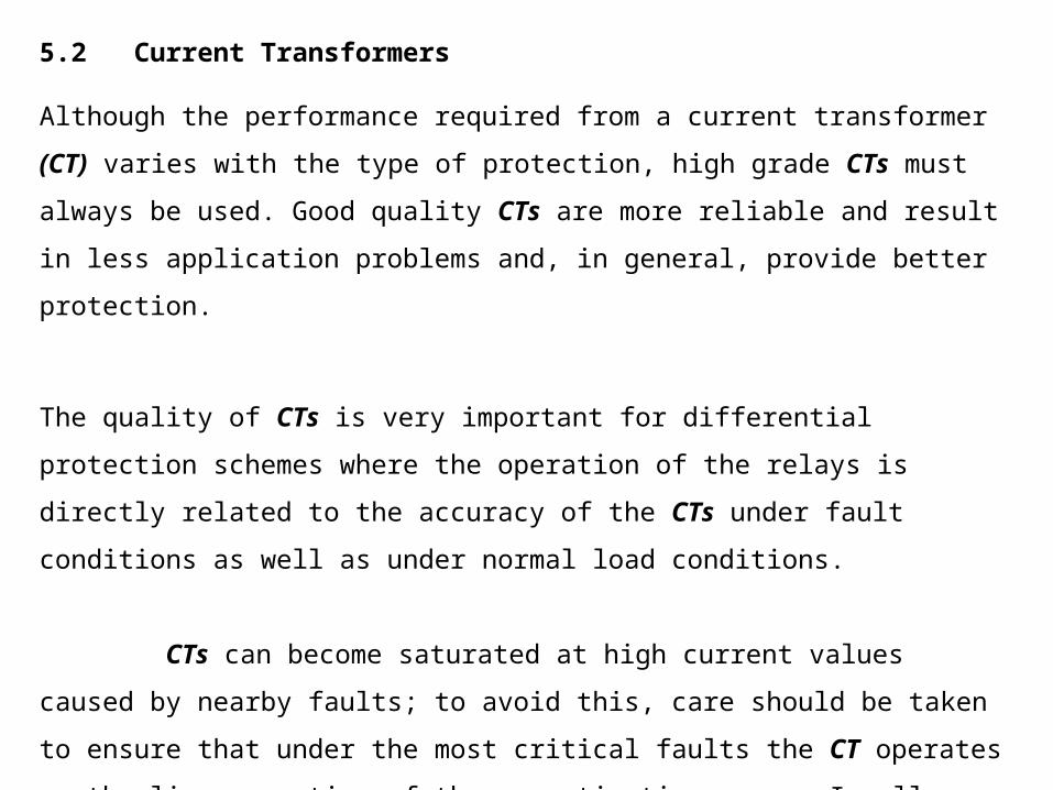
5.2 Current Transformers

Although the performance required from a current transformer (CT) varies with the

type of protection, high grade CTs must always be used. Good quality CTs are

more reliable and result in less application problems and, in general, provide better

protection.

The quality of CTs is very important for differential protection schemes where the

operation of the relays is directly related to the accuracy of the CTs under fault

conditions as well as under normal load conditions.

        CTs can become saturated at high current values caused by nearby faults; to

avoid this, care should be taken to ensure that under the most critical faults the CT

operates on the linear portion of the magnetization curve. In all these cases the CT

should be able to supply sufficient current so that the relay operates satisfactorily.

Design

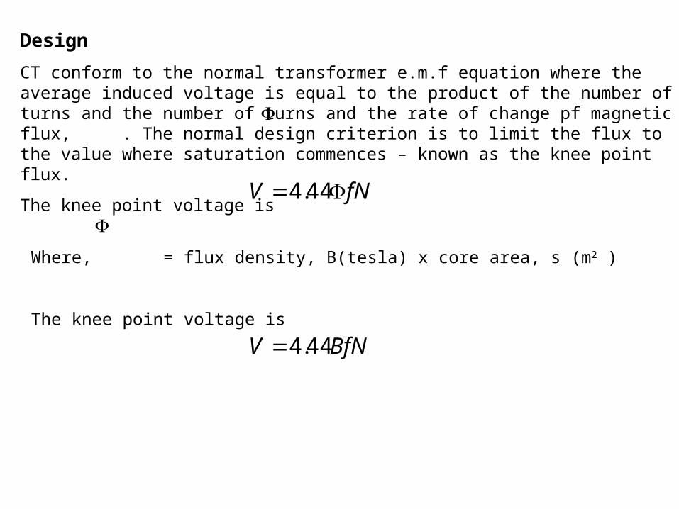
CT conform to the normal transformer e.m.f equation where the average induced voltage is equal to the product of the number of turns and the number of turns and the rate of change pf magnetic flux, . The normal design criterion is to limit the flux to the value where saturation commences – known as the knee point flux.

The knee point voltage is

fNV 44.4

Where, = flux density, B(tesla) x core area, s (m2 )

The knee point voltage is

BfNV 44.4

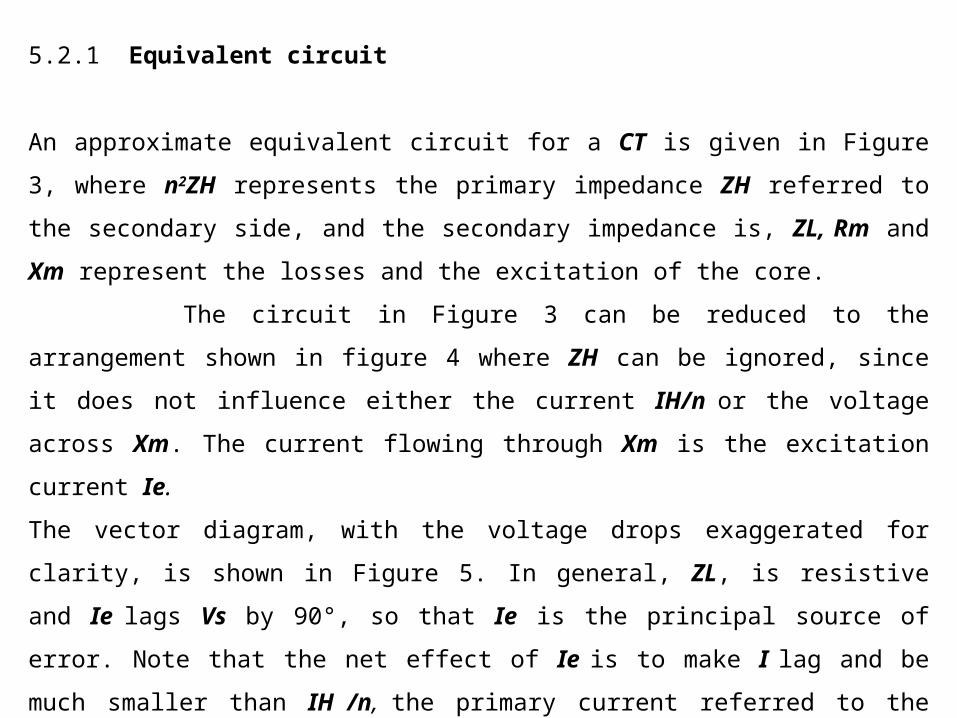
5.2.1 Equivalent circuit

An approximate equivalent circuit for a CT is given in Figure 3, where n2ZH

represents the primary impedance ZH referred to the secondary side, and the

secondary impedance is, ZL, Rm and Xm represent the losses and the excitation of

the core.

          The circuit in Figure 3 can be reduced to the arrangement shown in figure 4

where ZH can be ignored, since it does not influence either the current IH/n or the

voltage across Xm. The current flowing through Xm is the excitation current Ιe.

The vector diagram, with the voltage drops exaggerated for clarity, is shown in Figure

5. In general, ZL, is resistive and Ιe lags Vs by 90°, so that Ie is the principal source

of error. Note that the net effect of Ie is to make I lag and be much smaller than ΙH /n,

the primary current referred to the secondary side.

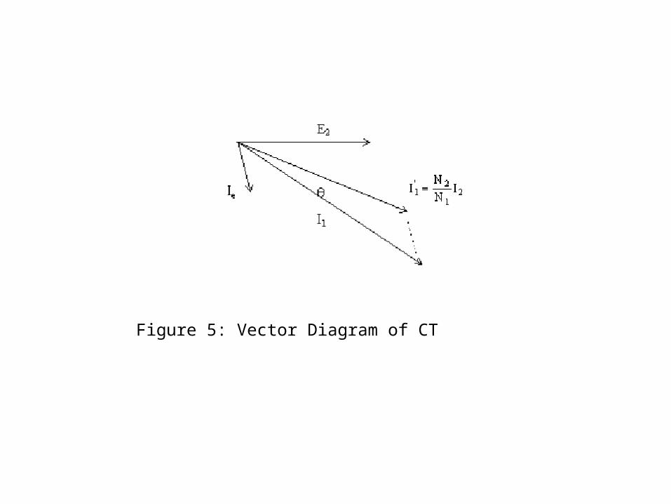
Figure 5: Vector Diagram of CT

5.2.2 CT Errors

The causes of errors in a CT are quite different to those associated with VTs. In

effect, the primary impedance of a CT does not have the same influence

On the accuracy of the equipment  it only adds an impedance in series with the

line, which can be ignored. The errors are principally due to the current which

circulates through the magnetizing branch.

          The magnitude error is the difference in magnitude between ΙH / n and IL

and is equal to Ir the component of Ie in line with k (see Figure 7).

The phase error, represented by θ, is related to Iq the component of Ie which is in

quadrature with IL. The values of the magnitude and phase errors depend on the

relative displacement between Ie and IL, but neither of them can exceed the

vectorial error it should be noted that a moderate inductive load, with Ie and IL

approximately in phase, has a small phase error and the excitation component

results almost entirely in an error in the magnitude.

5.2.3 AC Saturation

CΤ errors result from excitation current, so much so that, in order to check if a CT

is functioning correctly, it is essential to measure or calculate the excitation curve.

The magnetization current of a CT depends on the cross section and length of the

magnetic circuit, the number of turns in the windings, and the magnetic

characteristics of the material.

Thus, for a given CT, and referring to the equivalent circuit of Figure 3, it can be

seen that the voltage across the magnetization impedance, Es, is directly

proportional to the secondary current. From this it can be concluded that, when the

primary current and therefore the secondary current is increased, these currents

reach a point where the core commences to saturate and the magnetization

current becomes sufficiently high to produce an excessive error.

-continue-

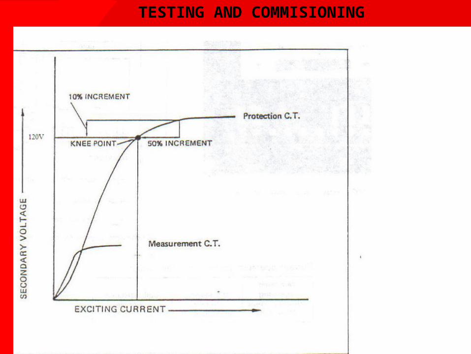
When investigating the behaviour of a CT, the excitation current should he

measured at various values of voltage  the so-called secondary injection test.

Usually, it is more convenient to apply a variable voltage to the secondary winding,

leaving the primary winding open-circuited. Figure 4.8a shows the typical

relationship between the secondary voltage and the excitation current determined in

this way.

       In European standards the point Κp on the curve is called the saturation or

knee point and is defined as the point at which an increase in the excitation

voltage of ten per cent produces an increase of 50 % in the excitation current

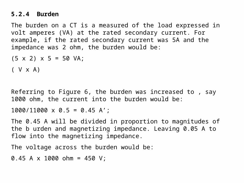
5.2.4 Burden

The burden on a CT is a measured of the load expressed in volt amperes (VA) at the rated secondary current. For example, if the rated secondary current was 5A and the impedance was 2 ohm, the burden would be:

(5 x 2) x 5 = 50 VA;

( V x A)

Referring to Figure 6, the burden was increased to , say 1000 ohm, the current into the burden would be:

1000/11000 x 0.5 = 0.45 A’;

The 0.45 A will be divided in proportion to magnitudes of the b urden and magnetizing impedance. Leaving 0.05 A to flow into the magnetizing impedance.

The voltage across the burden would be:

0.45 A x 1000 ohm = 450 V;

-continue-

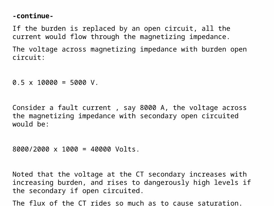
If the burden is replaced by an open circuit, all the current would flow through the magnetizing impedance.

The voltage across magnetizing impedance with burden open circuit:

0.5 x 10000 = 5000 V.

Consider a fault current , say 8000 A, the voltage across the magnetizing impedance with secondary open circuited would be:

8000/2000 x 1000 = 40000 Volts.

Noted that the voltage at the CT secondary increases with increasing burden, and rises to dangerously high levels if the secondary if open circuited.

The flux of the CT rides so much as to cause saturation.

-continue-

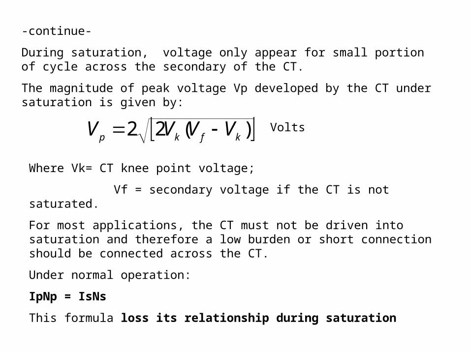
During saturation, voltage only appear for small portion of cycle across the secondary of the CT.

The magnitude of peak voltage Vp developed by the CT under saturation is given by:

)(22 kfkp VVVV Volts

Where Vk= CT knee point voltage;

Vf = secondary voltage if the CT is not saturated.

For most applications, the CT must not be driven into saturation and therefore a low burden or short connection should be connected across the CT.

Under normal operation:

IpNp = IsNs

This formula loss its relationship during saturation

5.2.5 Class and Type of CT

CT can be classified into three(3 major) categories:

• Measurement CTs

• General Purposes CTs

• Class X CTs

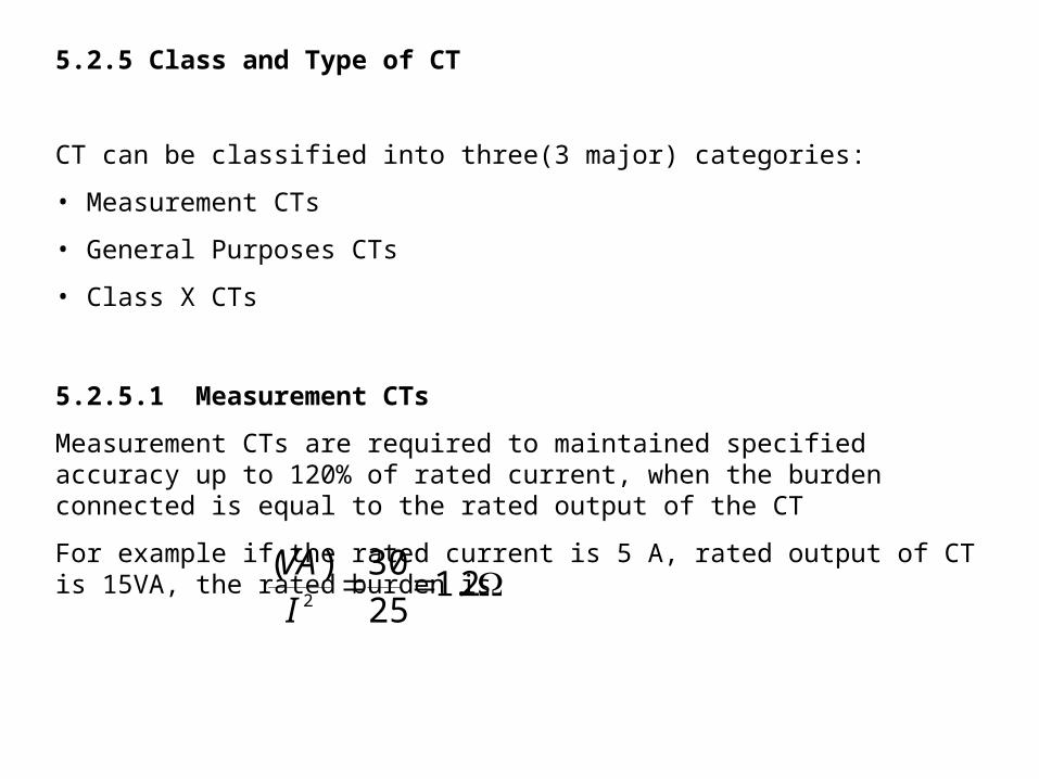
5.2.5.1 Measurement CTs

Measurement CTs are required to maintained specified accuracy up to 120% of rated current, when the burden connected is equal to the rated output of the CT

For example if the rated current is 5 A, rated output of CT is 15VA, the rated burden is

2.12530)(

2IVA

-continue-

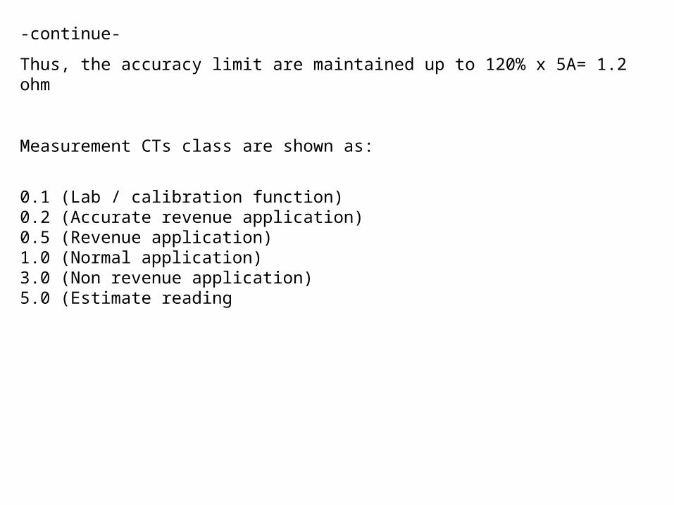
Thus, the accuracy limit are maintained up to 120% x 5A= 1.2 ohm

Measurement CTs class are shown as:

0.1 (Lab / calibration function)0.2 (Accurate revenue application)0.5 (Revenue application)1.0 (Normal application)3.0 (Non revenue application)5.0 (Estimate reading

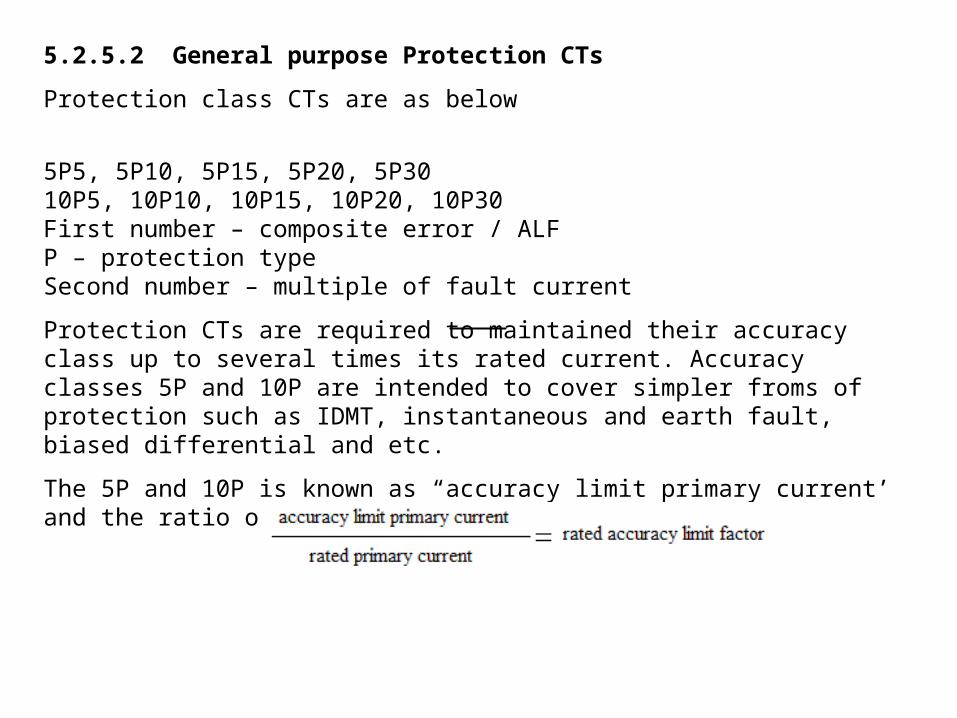
5.2.5.2 General purpose Protection CTs

Protection class CTs are as below

5P5, 5P10, 5P15, 5P20, 5P3010P5, 10P10, 10P15, 10P20, 10P30First number – composite error / ALFP – protection typeSecond number – multiple of fault current

Protection CTs are required to maintained their accuracy class up to several times its rated current. Accuracy classes 5P and 10P are intended to cover simpler froms of protection such as IDMT, instantaneous and earth fault, biased differential and etc.

The 5P and 10P is known as “accuracy limit primary current’ and the ratio of

-continue-

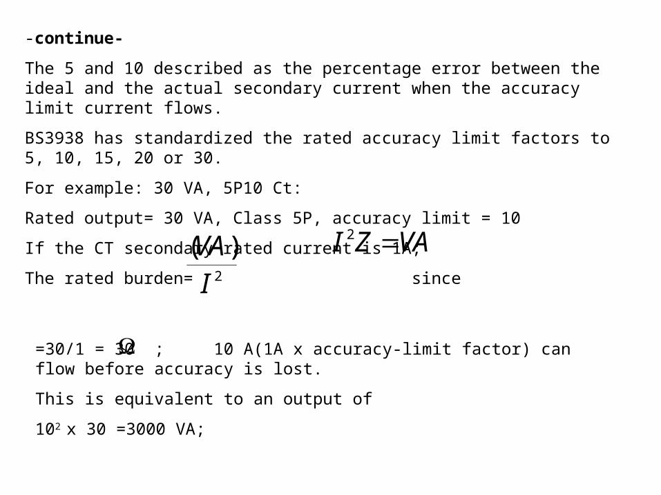
The 5 and 10 described as the percentage error between the ideal and the actual secondary current when the accuracy limit current flows.

BS3938 has standardized the rated accuracy limit factors to 5, 10, 15, 20 or 30.

For example: 30 VA, 5P10 Ct:

Rated output= 30 VA, Class 5P, accuracy limit = 10

If the CT secondary rated current is 1A;

The rated burden= since

2

)(IVA VAZI 2

=30/1 = 30 ; 10 A(1A x accuracy-limit factor) can flow before accuracy is lost.

This is equivalent to an output of

102 x 30 =3000 VA;

-continue-

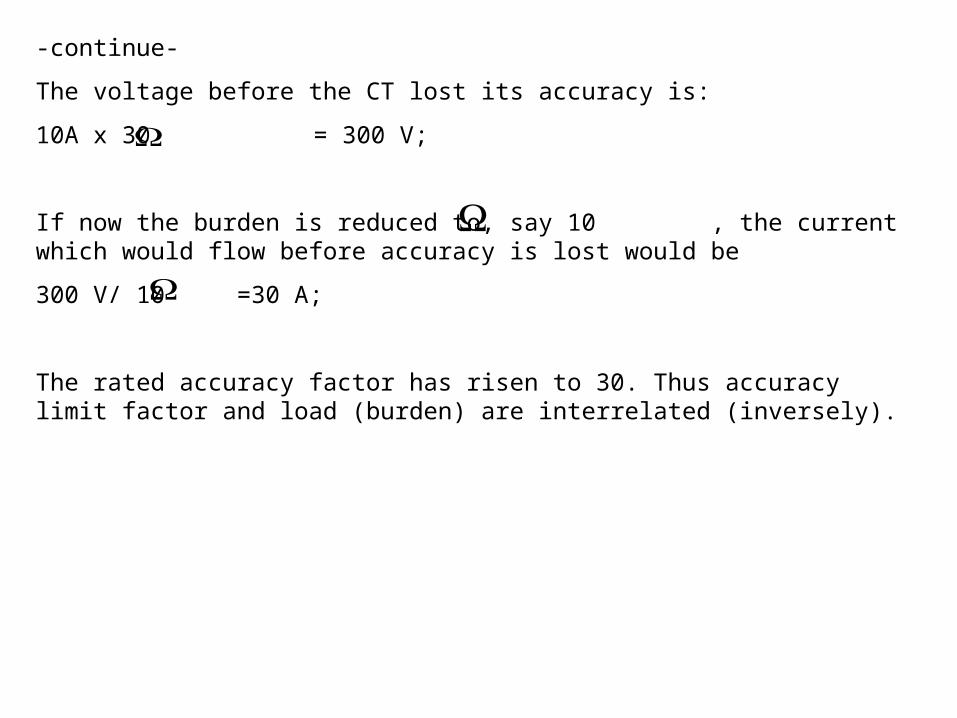
The voltage before the CT lost its accuracy is:

10A x 30 = 300 V;

If now the burden is reduced to, say 10 , the current which would flow before accuracy is lost would be

300 V/ 10 =30 A;

The rated accuracy factor has risen to 30. Thus accuracy limit factor and load (burden) are interrelated (inversely).

5.2.5.3 Class X CTs

BS 3938 defines class X CTs as required for special purpose applications. The performances specification is defined in terms of the following characteristics:

• rated primary current.

• turns ratio (with an error not exceeding 1.25%)

• rated knee-point EMF at maximum secondary turns.

• maximum exciting current at rated-knee point EMF

• resistance of the secondary winding at 75 degrees Celcius.

Class X Cts are usually applied when a high knee point is required to avoid saturation of the core. In protection context, they are usually categorised into two classes:

• Class A – designed to transform accurately without saturation up to a maximum fault current.

• Class B – for high impedance circulating current.

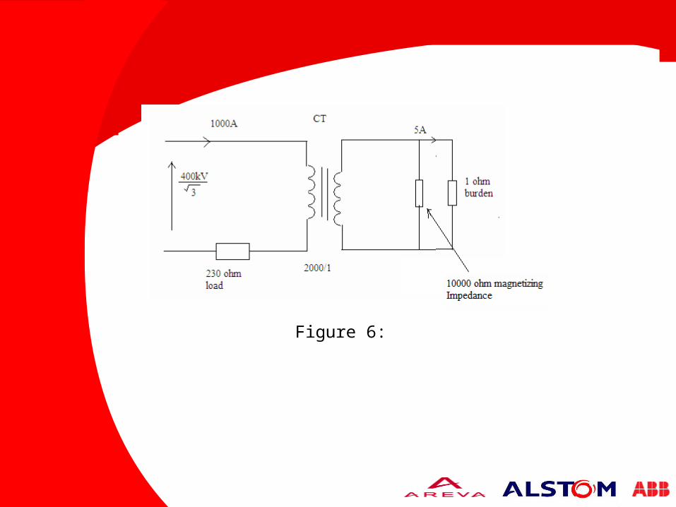
Figure 6:

TESTING AND COMMISIONING

DET310