The Power of Flexibility: Autonomous Agents That Conserve Energyin Commercial Buildings

by

Jun-young Kwak

A Dissertation Presented to theFACULTY OF THE USC GRADUATE SCHOOLUNIVERSITY OF SOUTHERN CALIFORNIA

In Partial Fulfillment of theRequirements for the DegreeDOCTOR OF PHILOSOPHY

(Computer Science)

November 2013

Copyright 2013 Jun-young Kwak

Acknowledgments

First and foremost, I would like to thank my advisor, Professor Milind Tambe, director of the

TEAMCORE research group. When I first joined, I literally had no idea what the definition of a

good advisor was, but it did not take too long for me to realize how lucky I was to have chosen to

work with Milind. Milind is a great advisor and one of the smartest and most creative people I

know. I hope that I can be as lively, enthusiastic, and energetic as him and someday be able to

command an audience as well as he can. Milind has been supportive and has given me the freedom

to pursue various projects without objection. He has also provided insightful discussions about the

research and has taught me new ways of thinking throughout my PhD tenure. In addition to our

academic collaboration, I greatly value the close personal support that Milind has provided over

the years. Quite simply I cannot imagine a better advisor.

Next, I would also like to thank my co-advisor, Professor Pradeep Varakantham at Singapore

Management University. He has been a great advisor, mentor, and friend ever since we met

at Carnegie Mellon University. I remember the short conversation with Pradeep at CMU has

eventually led me to USC and the TEAMCORE research group. I appreciate all of the time

and ideas he contributed to make my PhD experience productive and stimulating. The joy and

enthusiasm Pradeep has for his research was contagious and motivational for me throughout

ii

my time at USC. I am also thankful for the excellent example he has provided as a successful

researcher and professor.

Of course I gratefully acknowledge the other members of my dissertation guidance committee

for their time and valuable feedback on my research and thesis. In a line of research at the

intersection of many disciplines, my interdisciplinary committee could not have been more perfect

for shaping and pushing my research to the heights I have been able to achieve. My sincerest

gratitude to you all: Rajiv Maheswaran, Yu-Han Chang, Burcin Becerik-Gerber, and Wendy Wood.

During my time at USC I have also had the honor to work with many great researchers: Amos

Freedy, David Gerber, David Kempe, Matthew Taylor, Christopher Kiekintveld, Janusz Marecki,

Rong Yang, Nan Li, Timothy Hayes, Farrokh Jazizadeh, Geoffrey Kavulya, Laura Klein, and Onur

Sert.

I would also like to thank the rest of the TEAMCORE community, particularly those that I

have had the pleasure of spending my PhD career with: James Pita, Fei Fang, Thanh Nguyen,

Leandro Marcolino, Chao Zhang, Yundi Qian, Debarun Kar, Benjamin Ford, Haifeng Xu, Amulya

Yadav, Albert Jiang, Francesco Delle Fave, William Haskell, Bo An, Gal Kaminka, Nathan Schurr,

and Jagrut Sharma. I would particularly like to thank Manish Jain for being the best officemate

I could ask for, for all of your advice over the years, and for being a great friend even during

tough times in the PhD pursuit; Jason Tsai for being the sincere best friend who have spent infinite

nights together to have dinner/drinks while sharing many different thoughts, and for proofreading

my terrible writing millions of times without any complaints (I still owe you a lot of beers, so

whenever you feel thirsty, come down see me!); Zhengyu Yin for solving millions of mathematical

problems for me and for your great sense of humor; Matthew Brown for being a great neighbor

and friend in the apartment and in the office, for having provided valuable comments over the

iii

years, and for being a new drinks companion in K-town!; and Paul Scerri for being a source of

friendship as well as good advice and collaboration since we met at CMU. In addition, my time

at USC was made enjoyable in large part due to the many friends and groups that became a part

of my life: Maxim Makatchev, Mihail Pivtoraiko, Prasanna Velagapudi, William Yeoh and Chan

Seol.

Finally, I want to thank my family for all their love and encouragement. In particular, thank

you to my parents for supporting and undoubtedly believing me. Lastly, I would like to thank my

beautiful life companion Yu Jeong for coming into my life, being my best friend as well as a life

mentor. I could not express more of my gratefulness in words for your patience, kindness, faithful

support and love. Thank you.

iv

Table of Contents

Acknowledgments ii

List of Figures viii

List of Tables xi

Abstract xii

Chapter 1: Introduction 11.1 Problem Addressed . . . . . . . . . . . . . . . . . . . . . . . . . . . . . . . . . 21.2 Contributions . . . . . . . . . . . . . . . . . . . . . . . . . . . . . . . . . . . . 31.3 Guide to Thesis . . . . . . . . . . . . . . . . . . . . . . . . . . . . . . . . . . . 12

Chapter 2: Background 132.1 Markov Decision Problems . . . . . . . . . . . . . . . . . . . . . . . . . . . . . 132.2 Cooperative Game Theory and the Shapley Value . . . . . . . . . . . . . . . . . 142.3 Educational Building Testbeds . . . . . . . . . . . . . . . . . . . . . . . . . . . 16

2.3.1 The actual testbed building for SAVES . . . . . . . . . . . . . . . . . . 162.3.2 The actual testbed buildings for TESLA & THINC . . . . . . . . . . . . 18

2.4 Simulation Testbed . . . . . . . . . . . . . . . . . . . . . . . . . . . . . . . . . 192.4.1 Building Components . . . . . . . . . . . . . . . . . . . . . . . . . . . 202.4.2 Human Occupants . . . . . . . . . . . . . . . . . . . . . . . . . . . . . 232.4.3 Validation . . . . . . . . . . . . . . . . . . . . . . . . . . . . . . . . . . 25

2.5 Data Analysis . . . . . . . . . . . . . . . . . . . . . . . . . . . . . . . . . . . . 27

Chapter 3: SAVES 303.1 Agents in SAVES . . . . . . . . . . . . . . . . . . . . . . . . . . . . . . . . . . 303.2 Multi-objective MDPs . . . . . . . . . . . . . . . . . . . . . . . . . . . . . . . 333.3 BM-MDPs . . . . . . . . . . . . . . . . . . . . . . . . . . . . . . . . . . . . . . 353.4 Evaluation of SAVES . . . . . . . . . . . . . . . . . . . . . . . . . . . . . . . . 38

3.4.1 Simulation: Overall Evaluation . . . . . . . . . . . . . . . . . . . . . . 383.4.1.1 Result: Total Energy Consumption . . . . . . . . . . . . . . . 393.4.1.2 Result: Average Satisfaction Level . . . . . . . . . . . . . . . 41

3.4.2 Simulation: Multi-objective Optimization . . . . . . . . . . . . . . . . . 413.4.3 Real-world Test: Human Experiments . . . . . . . . . . . . . . . . . . . 44

v

Chapter 4: TESLA 484.1 TESLA Architecture . . . . . . . . . . . . . . . . . . . . . . . . . . . . . . . . 484.2 TESLA Algorithms . . . . . . . . . . . . . . . . . . . . . . . . . . . . . . . . . 49

4.2.1 Scheduling algorithms . . . . . . . . . . . . . . . . . . . . . . . . . . . 504.2.2 Identifying key meetings . . . . . . . . . . . . . . . . . . . . . . . . . . 59

4.3 Empirical Validation . . . . . . . . . . . . . . . . . . . . . . . . . . . . . . . . 614.3.1 Simulation Results . . . . . . . . . . . . . . . . . . . . . . . . . . . . . 61

4.3.1.1 Does flexibility help? . . . . . . . . . . . . . . . . . . . . . . 624.3.1.2 Online scheduling method with flexibility: Determining the

sample size in the TESLA SMILP . . . . . . . . . . . . . . . 634.3.1.3 Performance of online scheduling method with flexibility . . . 644.3.1.4 Performance of identifying key meetings . . . . . . . . . . . . 694.3.1.5 Considering the cancellation rate . . . . . . . . . . . . . . . . 70

4.4 Analysis: Savings due to TESLA . . . . . . . . . . . . . . . . . . . . . . . . . . 724.4.1 HVACs . . . . . . . . . . . . . . . . . . . . . . . . . . . . . . . . . . . 724.4.2 Lighting . . . . . . . . . . . . . . . . . . . . . . . . . . . . . . . . . . . 754.4.3 Electronics . . . . . . . . . . . . . . . . . . . . . . . . . . . . . . . . . 76

4.5 Human Subject Experiments . . . . . . . . . . . . . . . . . . . . . . . . . . . . 764.5.1 Survey for initial flexibility . . . . . . . . . . . . . . . . . . . . . . . . . 774.5.2 Survey for requested flexibility . . . . . . . . . . . . . . . . . . . . . . . 79

Chapter 5: THINC 825.1 Fair Division of Credit . . . . . . . . . . . . . . . . . . . . . . . . . . . . . . . 82

5.1.1 Approximate Shapley computation . . . . . . . . . . . . . . . . . . . . . 855.1.2 Approximate characteristic value computation . . . . . . . . . . . . . . . 88

5.2 THINC Rescheduling Algorithm . . . . . . . . . . . . . . . . . . . . . . . . . . 885.3 Empirical Validation . . . . . . . . . . . . . . . . . . . . . . . . . . . . . . . . 92

5.3.1 Shapley Value Evaluation . . . . . . . . . . . . . . . . . . . . . . . . . 935.3.1.1 Fair Division: Why Shapley Value? . . . . . . . . . . . . . . . 935.3.1.2 Approximation . . . . . . . . . . . . . . . . . . . . . . . . . . 93

5.3.2 Performance of replanning BM-MDP . . . . . . . . . . . . . . . . . . . 975.3.3 Deployed Application . . . . . . . . . . . . . . . . . . . . . . . . . . . 98

Chapter 6: Related Work 1016.1 Agent-based Systems in Energy . . . . . . . . . . . . . . . . . . . . . . . . . . 1026.2 Robust MDP and Multi-objective Optimization Techniques . . . . . . . . . . . . 1036.3 Resource Allocation and Scheduling . . . . . . . . . . . . . . . . . . . . . . . . 1056.4 Fair Division in Cooperative Game Theory . . . . . . . . . . . . . . . . . . . . . 106

6.4.1 Cooperative Game Theory in Energy Systems . . . . . . . . . . . . . . . 1066.4.2 Shapley Value and Approximation Techniques . . . . . . . . . . . . . . 107

6.5 Social Influence in Human Subject Studies . . . . . . . . . . . . . . . . . . . . . 109

Chapter 7: Conclusions 1117.1 Contributions . . . . . . . . . . . . . . . . . . . . . . . . . . . . . . . . . . . . 1127.2 Future Work . . . . . . . . . . . . . . . . . . . . . . . . . . . . . . . . . . . . . 115

vi

Bibliography 118

Appendix A: Properties of Shapley Value to Axiomatize Fairness 127

vii

List of Figures

2.1 Real Testbed Buildings . . . . . . . . . . . . . . . . . . . . . . . . . . . . . . . 16

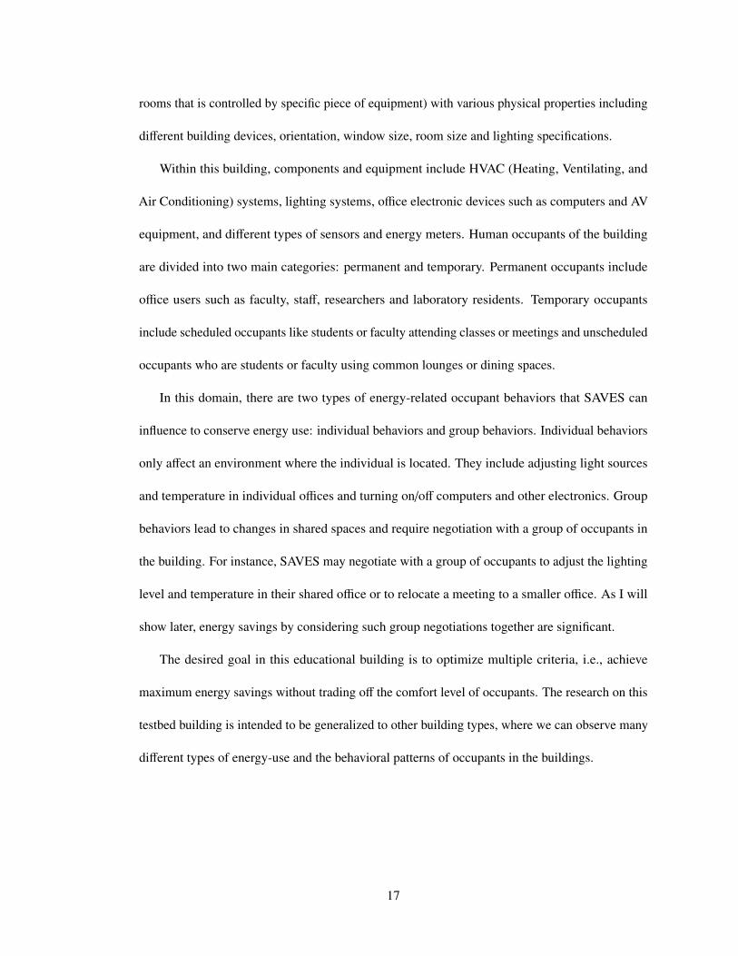
2.2 The current room reservation system at the testbed building . . . . . . . . . . . . 18

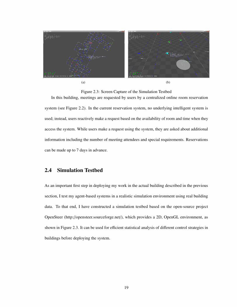
2.3 Screen Capture of the Simulation Testbed . . . . . . . . . . . . . . . . . . . . . 19

2.4 Parameter Values for Energy Calculation . . . . . . . . . . . . . . . . . . . . . . 21

2.5 RGL Floor Plan (2nd & 3rd floors of the testbed building) . . . . . . . . . . . . . 22

2.6 Actual Temperature Preference . . . . . . . . . . . . . . . . . . . . . . . . . . . 24

2.7 Energy Consumption Validation . . . . . . . . . . . . . . . . . . . . . . . . . . 25

2.8 Real data analysis (USC) . . . . . . . . . . . . . . . . . . . . . . . . . . . . . . 27

2.9 Real data analysis (SMU) . . . . . . . . . . . . . . . . . . . . . . . . . . . . . . 28

3.1 Agents & Communication Equipment in SAVES. An agent in SAVES sendsfeedback including energy use to occupants. . . . . . . . . . . . . . . . . . . . . 30

3.2 Performance Evaluation of SAVES . . . . . . . . . . . . . . . . . . . . . . . . . 40

3.3 Performance of BM-MDPs . . . . . . . . . . . . . . . . . . . . . . . . . . . . . 44

4.1 TESLA architecture: TESLA is a continuously running agent that supports fourkey features: (i) energy-efficient scheduling; (ii) identification of key meetings;(iii) learning of user preferences; and (iv) communication with users. . . . . . . . 48

4.2 Disjoint sets of R . . . . . . . . . . . . . . . . . . . . . . . . . . . . . . . . . . 51

viii

4.3 Energy savings: Actual - the amount of energy consumed in simulation based onthe past schedules obtained from the current manual reservation system; Random- energy consumption while randomly perturbing the starting time and locationof meeting requests from the same past schedules while keeping meeting timeduration; Optimal - Energy consumption measured in simulation based on optimalschedules computed from an SMILP with the fully known meeting request set andfull flexibility . . . . . . . . . . . . . . . . . . . . . . . . . . . . . . . . . . . . 62

4.4 Scalability and accuracy while varying the number of samples (N) . . . . . . . . 63

4.5 Energy savings while varying flexibility (USC) . . . . . . . . . . . . . . . . . . 64

4.6 Energy savings while varying flexibility (SMU) . . . . . . . . . . . . . . . . . . 68

4.7 Average energy improvement while considering the cancellation rate of meetingrequests . . . . . . . . . . . . . . . . . . . . . . . . . . . . . . . . . . . . . . . 71

4.8 Energy savings by TESLA: the percentage of energy savings per each energyconsumer and factor . . . . . . . . . . . . . . . . . . . . . . . . . . . . . . . . . 72

4.9 Energy saving analysis: room size . . . . . . . . . . . . . . . . . . . . . . . . . 73

4.10 Energy savings only by HVACs (Non-peak Time) . . . . . . . . . . . . . . . . . 73

4.11 Screenshot of online survey: people were asked to indicate their meeting requestsand flexibility. . . . . . . . . . . . . . . . . . . . . . . . . . . . . . . . . . . . . 77

4.12 Diversity of people’s flexibility . . . . . . . . . . . . . . . . . . . . . . . . . . . 79

5.1 THINC architecture . . . . . . . . . . . . . . . . . . . . . . . . . . . . . . . . . 82

5.2 Illustrative example: Li & Ti mean available rooms and time slots, respectively. Eachmeeting request ri has a set of preferred locations and time, which indicates location andtime flexibility. . . . . . . . . . . . . . . . . . . . . . . . . . . . . . . . . . . . . 84

5.3 Runtime comparison – S: Sampling (# of samples), C: Caching, P: Partitioning (#of partitions), L: LP Relaxation . . . . . . . . . . . . . . . . . . . . . . . . . . . 94

5.4 Solution quality . . . . . . . . . . . . . . . . . . . . . . . . . . . . . . . . . . . . 95

5.5 Average deviation (%) . . . . . . . . . . . . . . . . . . . . . . . . . . . . . . . . 95

5.6 Efficiency violation (%) . . . . . . . . . . . . . . . . . . . . . . . . . . . . . . . . 96

5.7 Solution quality . . . . . . . . . . . . . . . . . . . . . . . . . . . . . . . . . . . . 96

ix

5.8 Measured users’ flexibility . . . . . . . . . . . . . . . . . . . . . . . . . . . . . . 98

x

List of Tables

2.1 Parameter Description for Energy Calculation . . . . . . . . . . . . . . . . . . . 22

2.2 Parameter Values for Energy Calculation . . . . . . . . . . . . . . . . . . . . . . 23

2.3 Energy consumption validation (kWh) . . . . . . . . . . . . . . . . . . . . . . . 26

2.4 Meeting request arrival distribution . . . . . . . . . . . . . . . . . . . . . . . . . 27

3.1 Average Maximum Regret Comparison . . . . . . . . . . . . . . . . . . . . . . 42

3.2 Example of the Meeting Relocation Negotiation . . . . . . . . . . . . . . . . . . 42

3.3 Lighting Negotiation Results (*: p < 0.05) . . . . . . . . . . . . . . . . . . . . . 46

4.1 Performance comparison between SAA and myopic . . . . . . . . . . . . . . . . 65

4.2 % of optimal energy savings: varying αT , αL, and p f (USC) . . . . . . . . . . . 67

4.3 Percentage of optimal energy savings: varying αd (USC) . . . . . . . . . . . . . 67

4.4 Percentage of optimal energy savings: varying αd (SMU) . . . . . . . . . . . . . 69

4.5 Energy improvement of identified key meetings (%) . . . . . . . . . . . . . . . . 69

4.6 Basic Profile Questionnaire . . . . . . . . . . . . . . . . . . . . . . . . . . . . . 78

4.7 Survey I: Questionnaire . . . . . . . . . . . . . . . . . . . . . . . . . . . . . . . 78

4.8 Flexibility manipulation with various feedback (%) . . . . . . . . . . . . . . . . 79

5.1 Runtime Comparison (hours) – In conjunction with caching & LP relaxation (# of meetings:100) . . . . . . . . . . . . . . . . . . . . . . . . . . . . . . . . . . . . . . . . . 94

5.2 Rescheduling real meetings: uncertainty in user reactions . . . . . . . . . . . . . . . 99

xi

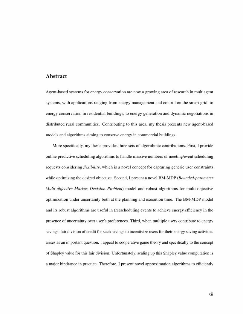
Abstract

Agent-based systems for energy conservation are now a growing area of research in multiagent

systems, with applications ranging from energy management and control on the smart grid, to

energy conservation in residential buildings, to energy generation and dynamic negotiations in

distributed rural communities. Contributing to this area, my thesis presents new agent-based

models and algorithms aiming to conserve energy in commercial buildings.

More specifically, my thesis provides three sets of algorithmic contributions. First, I provide

online predictive scheduling algorithms to handle massive numbers of meeting/event scheduling

requests considering flexibility, which is a novel concept for capturing generic user constraints

while optimizing the desired objective. Second, I present a novel BM-MDP (Bounded-parameter

Multi-objective Markov Decision Problem) model and robust algorithms for multi-objective

optimization under uncertainty both at the planning and execution time. The BM-MDP model

and its robust algorithms are useful in (re)scheduling events to achieve energy efficiency in the

presence of uncertainty over user’s preferences. Third, when multiple users contribute to energy

savings, fair division of credit for such savings to incentivize users for their energy saving activities

arises as an important question. I appeal to cooperative game theory and specifically to the concept

of Shapley value for this fair division. Unfortunately, scaling up this Shapley value computation is

a major hindrance in practice. Therefore, I present novel approximation algorithms to efficiently

xii

compute the Shapley value based on sampling and partitions and to speed up the characteristic

function computation.

These new models have not only advanced the state of the art in multiagent algorithms, but

have actually been successfully integrated within agents dedicated to energy efficiency: SAVES,

TESLA and THINC. SAVES focuses on the day-to-day energy consumption of individuals and

groups in commercial buildings by reactively suggesting energy conserving alternatives. TESLA

takes a long-range planning perspective and optimizes overall energy consumption of a large

number of group events or meetings together. THINC provides an end-to-end integration within

a single agent of energy efficient scheduling, rescheduling and credit allocation. While SAVES,

TESLA and THINC thus differ in their scope and applicability, they demonstrate the utility of

agent-based systems in actually reducing energy consumption in commercial buildings.

I evaluate my algorithms and agents using extensive analysis on data from over 110,000 real

meetings/events at multiple educational buildings including the main libraries at the University

of Southern California. I also provide results on simulations and real-world experiments, clearly

demonstrating the power of agent technology to assist human users in saving energy in commercial

buildings.

xiii

Chapter 1: Introduction

Limited availability of energy sources has led to the need to develop efficient measures of conserv-

ing energy and has raised broad interests in building agent-based systems for real world energy

applications. Motivated by this need, researchers in the multiagent community have successfully

developed agent-based systems for saving energy both in the smart grid and in buildings [Stein

et al., 2012; Mamidi et al., 2012b; Kamboj et al., 2011; Ramchurn et al., 2011; Rogers et al., 2011;

Voice et al., 2011; Bapat et al., 2011; Sou et al., 2011; Xiong et al., 2011].

More specifically, sustainable production, delivery and use of energy in the smart grid and

buildings has now become an important challenge. The distributed nature of the energy grid

and the individual interests of users makes multiagent modeling an appropriate approach for

this problem. For instance, intelligent systems in the smart grid efficiently predict the use of

energy and dynamically optimize its delivery [Vytelingum et al., 2010; Ramchurn et al., 2011].

A game-theoretic framework for modeling storage devices in large-scale systems where each

storage device is owned by a self-interested agent that aims to maximize its monetary profit [Voice

et al., 2011; Vandael et al., 2011]. Multiagent systems have been also widely employed to

model home automation systems (or smart homes) and simulating control algorithms to evaluate

performance [Rogers et al., 2011; Abras et al., 2006; Conte and Scaradozzi, 2003; Roy et al.,

1

2006]. This research has given rise to a new area of agent-based systems for energy conservation.

Contributing to this area, my thesis presents new agent-based models and algorithms aiming

at conserving energy in commercial (including office and educational) buildings, given their

significant energy consumption.

1.1 Problem Addressed

Reducing energy consumption is an important goal for sustainability. Conserving energy in

commercial buildings is important as these buildings are responsible for significant energy con-

sumption. In 2008, commercial buildings in the U.S. consumed 18.5 QBTU1, representing 46.2%

of building energy consumption and 18.4% of U.S. energy consumption [U.S. Department of

Energy, 2010]. Such rapid growth in energy usage from commercial buildings has made the need

for systems that aid in reducing energy consumption a top priority.

Researchers have been developing multiagent systems to conserve energy for deployment in

smart grids and buildings [Kamboj et al., 2011; Mamidi et al., 2012a; Miller et al., 2012; Ramchurn

et al., 2011; Rogers et al., 2011; Stein et al., 2012; Bapat et al., 2011; Sou et al., 2011; Xiong et al.,

2011]. However, their work has been done with a particular focus on residential buildings, and that

work does not directly apply to commercial buildings. For instance, those approaches focus on

flexible scheduling of household appliances, or presenting techniques for home automation [Bapat

et al., 2011; Mohsenian-Rad and Leon-Garcia, 2010; Sou et al., 2011; Wang et al., 2009; Xiong

et al., 2011]. More discussion will follow in the related work section.1QBTU indicates Quadrillion BTU, which is used as the common unit to explain global energy use. 1 BTU =

0.00029 kWh.

2

While the goal of a sustainable energy system is the same in both commercial and residential

buildings (i.e., efficiently conserving energy), three unique research challenges should be simulta-

neously addressed for successfully saving energy in commercial buildings. First, algorithms should

be able to handle massive meetings/events schedules while focusing on conserving energy and

considering the given human models. Second, the types of energy-related behaviors in commercial

buildings are different from residential buildings and require agents to negotiate with groups of

people for guiding their behaviors to conserve further energy (e.g., scheduling group activities

such as meetings). Thus, energy systems in commercial buildings should harness changes in

people’s energy related behaviors while ensuring a balance of energy savings and comfort (i.e.,

multi-objective optimization). However, there may be uncertainty in people’s preferences regard-

ing such group activities, and thus the system may not be able to directly learn those preference

models (i.e., model uncertainty). Third, algorithms should also ensure that proper credit is given

based on people’s true contribution to the energy savings in order to effectively motivate people in

a shared place (i.e., fair credit).

1.2 Contributions

The key insight underlying my thesis is that adding flexibility to meeting/event schedules in

commercial buildings can lead to significant energy savings. Such savings can then be divided

amongst the group of people who provided flexibility to incentivize further savings. In the long

run, via my agent-based systems, people are sustainably encouraged to provide more flexibility by

incentives that come from savings caused by such flexibility. In this context, my thesis presents new

agent-based models and algorithms aiming to conserve energy in commercial buildings. My three

3

algorithmic contributions are: (i) performing predictive scheduling on massive number of group

events while considering human users’ behavior preferences and constraints; (ii) interacting with

human users to gain further savings by changing their given behavior and in particular scheduling

preferences; and (iii) dividing up such credit of energy savings in a fair manner as part of an

incentive mechanism.

The first contribution of my thesis handles online predictive scheduling of massive numbers

of dynamically arriving and uncertain meetings/events while considering flexibility, which is a

novel concept for capturing generic user constraints [Kwak et al., 2013a,b]. In reality, uncertainty

is prevalent in the context of scheduling due to lack of accurate prediction models and data.

Therefore, it is of crucial importance to develop systematic methods to address the problem of

scheduling under uncertainty, in order to create efficient and reliable schedules while satisfying the

given objective. To that end, I propose a novel robust optimization approach for scheduling a large

number of meetings while considering (i) flexibility in meeting requests over time, location and

deadlines; and (ii) user preferences with respect to multiple objectives (e.g., energy and comfort).

More specifically, I provide the following algorithmic contribution: a two-stage stochastic mixed

integer linear program (SMILP) for energy-efficient scheduling of incrementally/dynamically

arriving meetings and events.

Stochastic programming has provided a framework for modeling optimization problems that

involve uncertainty [Beale, 1955; Dantzig, 1955; Kall and Wallace, 1994; Shapiro et al., 2009].

Whereas deterministic optimization problems are formulated with known parameters, real-world

problems almost invariably include some unknown parameters. To address this challenge, I

specifically formulate the scheduling problem as a two-stage stochastic program. In general, in a

two-stage stochastic program, the first stage variables are decided before the actual realization of

4

the uncertain parameters are known. Afterward, once the random events have exhibited themselves,

further decisions can be made by selecting the values of the second stage. The objective of the

SMILP above is to choose the optimal first stage variables in a way that the sum of first stage costs

and the expected value of the second stage or recourse costs is minimized. I then use the sample

average approximation (SAA) method [Ahmed et al., 2002; Pagnoncelli et al., 2009] to solve the

given SMILP. The main idea of the SAA approach to solve stochastic programs is to approximate

the expected value of the second stage cost by the weighted average function with the sample

realizations of the random vector that determines future meeting requests. The obtained sample

average approximation of the stochastic program is then solved using a standard branch and bound

algorithm such as those implemented in commercial integer programming solvers. For evaluation,

I compared the simulation results in energy savings achieved by the proposed predictive scheduling

algorithm against real-world data. These results show that my predictive scheduling algorithms

can potentially offer significant saving benefits in general scheduling domains where schedule

flexibility plays a key role for such savings.

The second contribution of my thesis provides a robust MDP (Markov Decision Problem)

model and algorithms to effectively reschedule group activities such as meetings/events for saving

energy while considering multiple objectives as well as uncertainty both at planning and execution

time [Kwak et al., 2012a,b]. In fact, in a complex domain, three challenges need to be considered.

First, there are inherently multiple competing objectives like limited energy supplies, and demands

to satisfy occupants’ comfort levels. This makes the problem harder as I need to explicitly consider

multi-objective optimization techniques. Second, as human occupants are directly involved in the

optimization procedures, understanding human behavior models and simultaneously reasoning

about such model uncertainty in the domain are essential. Third, while the offline policy is being

5

executed, there might be unexpected situations that were not captured at planning time. This

combination of challenges (multiple objectives and planning & execution-time uncertainty) has not

been considered in previous MDP algorithms [Chatterjee et al., 2006; Delgado et al., 2009; Givan

et al., 2000; Ogryczak et al., 2011]. Specifically, I present a novel model and robust algorithms:

• BM-MDP (Bounded-parameter Multi-objective MDP) that explicitly models multiple objec-

tives as well as uncertainty over people’s preferences

• robust algorithms to solve BM-MDPs and dynamic replanning methods for handling uncer-

tainty at execution time

BM-MDPs are a hybrid of MO-MDPs (Multi-Objective MDPs) Chatterjee et al. [2006];

Ogryczak et al. [2011] and BMDPs (Bounded-parameter MDPs) Givan et al. [2000]. Thus,

BM-MDPs are defined as an MDP where the reward function has been replaced by a vector

of rewards and upper and lower bounds on transition probabilities and rewards are provided as

closed real intervals. To optimally solve the given BM-MDPs, I provide algorithms based on

robust value iteration [Bagnell et al., 2001], which relies on a minimax approach, to obtain a

well-balanced solution across multiple objectives under model uncertainty. As I will show in the

results, BM-MDPs generate robust solutions while considering multiple objectives and model

uncertainty at planning time.

In practice, however, BM-MDPs may still not always capture unexpected situations that arise

while the BM-MDP policy is being executed. To handle such execution-time uncertainty, I also

provide the execution-centric replanning algorithms that heuristically replan the BM-MDP policy

while considering dynamic situations at execution time. As I will show in the evaluation section,

this replanning approach performs better than two other alternatives.

6

The final contribution of my thesis addresses fair division of credit using concepts of coopera-

tive game theory. When multiple users contribute to energy savings, fair division of credit for such

savings arises as an important question. Given the total amount of energy savings, what would

be a fair method to divide up credit of such energy savings? For instance, if each user were to

be compensated from a fixed portion of the entire group savings to incentivize further savings,

such equal division among all users would imply that those who made an extra effort get the same

credit as those who contributed little or nothing, which may not be perceived as fair [Nisan, 2007;

Nagarajan et al., 2010].

I appeal to cooperative game theory and specifically to the concept of Shapley value for this

fair division [Shapley, 1953]. While the Shapley value mathematically computes fair individual

allocations and holds desirable theoretical properties such as efficiency, symmetry, linearity, etc.,

its limitation in scale is a major hindrance in practice [Nisan, 2007; Castro et al., 2009; Fatima et al.,

2008]. The Shapley value is based on the marginal contribution of each agent in a permutation, i.e.,

the amount of additional utility generated when that agent joins the coalition of her predecessors

in the permutation. And thus, the marginal contribution of each individual agent to every subset of

a given coalition should be considered. Furthermore, computing the marginal contribution in each

permutation (i.e., the characteristic function value) requires the exact computation of the energy

savings, which is computationally challenging. Thus, I provide a novel algorithmic contribution

for scaling up the overall computations:

• approximation algorithms to efficiently compute the Shapley value based on sampling and

partitions

• an LP (linear program) relaxation method to speed up the characteristic function computation

7

Some studies suggest the use of sampling methods to approximate the Shapley value [Castro

et al., 2009]. Motivated by this prior work, I provide an approximate algorithm for the polynomial-

time calculation of the Shapley value based on sampling. An additional caching technique is used

to further speed-up the Shapley value computation by storing each evaluation of the characteristic

function. I also present the partition-based technique to decompose the entire agent set into smaller

independent subsets, which reduce the overall computational burden.

Next, in practice, the characteristic function computation itself is often computationally

intensive as it requires complex mathematical formulations (e.g., a mixed integer linear program

(MILP)) to be solved repeatedly. Thus, I present an LP relaxation method to speed up the

characteristic function computation by relaxing constraints of key integer decision variables. For

the corresponding LP relaxation to be practical, I also provide a rounding scheme for the resulting

continuous solution. As I will show in the evaluation section, these approximations allow efficient

computations of fair individual allocations in a large-scale saving game in the real-world. I

also show that different combinations of these approximations can be chosen under particular

circumstances while considering the tradeoff between solution quality and runtime.

My algorithmic contributions discussed above have been successfully integrated within agents

dedicated to energy efficiency. My thesis specifically introduces SAVES (Sustainable multi-Agent

building application for optimizing Various objectives including Energy and Satisfaction) [Kwak

et al., 2012a,b], TESLA (Transformative Energy-saving Schedule-Leveraging Agent) [Kwak

et al., 2013a,b] and THINC (agent Tool for Human INcentivization and Cooperation), illustrating

the potential for energy savings in commercial buildings. SAVES focuses on the day-to-day

energy-consumption of single individual or single group activity in commercial buildings, to be

reactive in suggesting energy conserving alternative to that individual or group. SAVES uses Ralph

8

& Goldy Lewis Hall (RGL) at the University of Southern California as a testbed building. More

specifically, SAVES provides the following key novelties:

• jointly performed with the university facility management team, SAVES is based on actual

occupant preferences and schedules, actual energy consumption and loss data, real sensors

and hand-held devices, etc.

• SAVES addresses novel scenarios that require agents to negotiate with groups of building

occupants to conserve energy; previous work has typically focused on agents’ negotiation

with individual occupants [Abras et al., 2008; Mo and Mahdavi, 2003].

• SAVES focuses on non-residential buildings, which offer new opportunities for energy

conservation. In particular, since occupants may follow a more regular schedule, it allows

SAVES to plan ahead for energy conservation.

• As mentioned previously, SAVES uses a novel algorithm for generating optimal BM-MDP

policies that explicitly considers multiple objective optimization (energy and personal

comfort) as well as uncertainty over occupant preferences when negotiating for energy

reduction.

Then, I provide three sets of evaluation results for SAVES. First, I constructed a detailed

simulation testbed, with details all the way down to individual electrical outlets in the targeted

building and variations in solar gain per day; and then validated this simulation. Within this

simulation testbed, I show that SAVES substantially reduces the overall energy consumption

compared to existing control methods while achieving comparable satisfaction level of occupants.

Second, I show the benefits of BM-MDPs by showing that it gives a well-balanced solution

9

while considering multiple objectives. Third, as a real-world test, I provide results of a human

subject study where SAVES is shown to lead human occupants to significantly reduce their energy

consumption in real buildings.

On the other hand, TESLA takes a long-range planning perspective and optimizes overall

energy consumption of a large number of group events or meetings together. TESLA is a goal-

seeking (to save energy), continuously running autonomous agent. Users in a commercial building

continuously submit meeting requests to TESLA while indicating flexibility in their meeting

preferences. TESLA schedules these meetings in the most energy efficient manner while ensuring

user comfort; but in cases where shifting meeting times can lead to significant savings, TESLA

interacts with users to request such a shift. More specifically, TESLA provides the following key

novelties:

• As previously mentioned, TESLA presents online scheduling algorithms using the sample

average approximation (SAA) method to solve a two-stage stochastic mixed integer linear

program (SMILP). This SMILP considers the flexibility of people’s preferences for energy-

efficient scheduling of incrementally/dynamically arriving meetings and events.

• TESLA also includes an algorithm to effectively identify key meetings that could lead

to significant energy savings by adjusting their flexibility while considering uncertainty

regarding people’s interactions.

For evaluation, I used a public domain simulation testbed [Kwak et al., 2012a,b], fitted it with

details of the testbed building, and compared the simulation results against real-world energy

usage data. TESLA was extensively evaluated on data gathered from over 110,000 meetings held

at nine campus buildings during an eight month period in 2011–2012 at the University of Southern

10

California (USC) and Singapore Management University (SMU), and an extensive analysis of the

energy saving results achieved by TESLA is provided. These analyses and results show that, in a

validated simulation using the testbed building, TESLA is projected to save about 94,000 kWh of

energy (roughly $18K) annually.

Lastly, THINC is the first agent integrating (i) energy-efficient scheduling of user meeting

requests while considering flexibility, (ii) rescheduling of key meetings for more energy savings,

and (iii) fair credit allocations based on Shapley value to incentivize users for their energy saving

activities (i.e., providing flexibility). More specifically, THINC provides the following key

novelties:

• THINC computes fair division of credits from energy savings. For this fair division, THINC

uses novel algorithmic advances for efficient computation of Shapley value mentioned

earlier.

• THINC includes a novel robust algorithm to optimally reschedule identified key meetings

addressing user interaction uncertainty.

For the evaluation, I built upon the simulation testbed by using a large data set of real meeting

requests and building statistics collected from the testbed building at USC. As a real-world test, I

actually deployed THINC at the Doheny library at USC in a limited fashion, collected real user’s

flexibility and their input, and demonstrated that THINC has significant potential to produce real

energy savings in commercial buildings.

11

1.3 Guide to Thesis

This thesis is organized in the following way. Chapter 2 introduces necessary background for

the research presented in this thesis. Chapter 3 presents robust algorithms for BM-MDPs, and

shows its extension to be applied in SAVES and the corresponding experimental results. Chapter 4

presents the robust optimization optimization framework for computing energy-efficient schedules

in TESLA and the corresponding experimental results. Chapter 5 describes THINC for handling

more realistic situations in order to be deployed in the real-world. Chapter 6 presents related work.

And finally, Chapter 7 concludes the thesis and presents issues for future work.

12

Chapter 2: Background

In this chapter, I provide a brief background regarding MDPs in Section 2.1, and discuss concepts

of cooperative game theory and specifically the Shapley value in Section 2.2. Next, I describe

two different sets of real testbed buildings in Section 2.3 and a simulation testbed in Section 2.4.

As a simulation environment is a main testbed to evaluate algorithms presented in my thesis, I

also provide the detailed evaluation results of the simulation environment using real building and

energy data in Section 2.4.3. Finally, in Section 2.5, I present a data analysis on massive number

of meeting requests collected from real testbed buildings described in Section 2.3.

2.1 Markov Decision Problems

Planning under uncertainty is fundamental to solving many important real-world problems, includ-

ing applications in robotics, network routing, scheduling, and financial decision making. Markov

Decision Problems (MDPs) [Puterman, 2009] provide a mathematical framework for modeling

these tasks and for deriving optimal solutions, which are described by a tuple 〈S , A,T,R〉:

• S = {s1, ..., sk} is a finite set of states.

• A is the finite set of actions of agent.

13

• T : S × A × S 7→ R is the transition function, where T (s′|s, a) is the transition probability

from s to s′ if an action a is executed.

• R : S × A × S 7→ R is the reward function, where R(s, a, s′) is the reward agents get by

taking a from s and reaching s′.

The MDP is to obtain a policy with the highest expected reward/value and can be solved by

the following linear program (LP) formulation to find the optimal policy:

min V(s) (2.1)

s.t. V(s) ≥ R(s, a) + γ∑s′∈S

T (s, a, s′) · V(s′), (2.2)

0 ≤ γ < 1 (2.3)

where V is a value function, and γ is a discount factor.

2.2 Cooperative Game Theory and the Shapley Value

Cooperative game theory [Nisan, 2007; Leyton-Brown and Shoham, 2008] allows players to band

together and form coalitions. Formally, a cooperative game is defined by a pair (N, v), where

N = {1, 2, . . . , n} is a set of players, and v is a characteristic function specifying the value created

of different subsets (i.e., coalitions) of the players in the game. Specifically, the characteristic

function, v(S ), associates with every subset S of N a value v(S ), the value of the coalition S .

In a cooperative game, we often want to encourage the grand coalition N to form. The

challenge is to allocate the overall payoff v(N) among the players in a fair way so that they

14

will not deviate and form their own coalitions. Several solution concepts such as the Shapley

value [Shapley, 1953], the core [Gillies, 1959], and the nucleolus [Schmeidler, 1969] exist to guide

allocation. These solution concepts all find a vector x ∈ RN that represents the allocation to each

player.

The Shapley value yields a unique allocation x(v) = φ(N, v) that is also fair. Specifically, the

Shapley value satisfies the efficiency, symmetry, dummy player, and additivity properties which

axiomatize fairness. Other concepts in cooperative game theory such as the core and the nucleolus

focus on yielding stable outcomes, but not necessarily fairness, which is of key interest in our

work. Furthermore, the existence and uniqueness of the core are not guaranteed.

I use two (equivalent) definitions of Shapley value in our paper. The Shapley value is obtained

by averaging the marginal contributions over all possible coalitions. Specifically, the Shapley

value for player i is:

φi(N, v) =

n−1∑s=0

s!(n − 1 − s)!n!

∑S⊆N\{i},|S |=s

(v(S ∪ {i}) − v(S )) (2.4)

where φi(N, v) is the savings due to i ∈ N in the game (N, v).

An alternative definition of the Shapley value can be expressed in terms of all possible orders

of the players N. Let O : {1, . . . , n} → {1, . . . , n} be a permutation that assigns to each position

k the player O(k). Let us denote by π(N) the set of all possible permutations with player set N.

Given a permutation O, let us denote by Pi(O) the set of predecessors of the player i in the order O

15

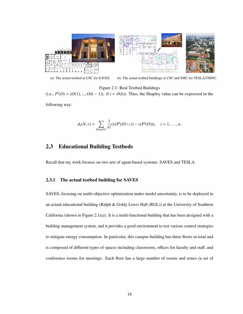
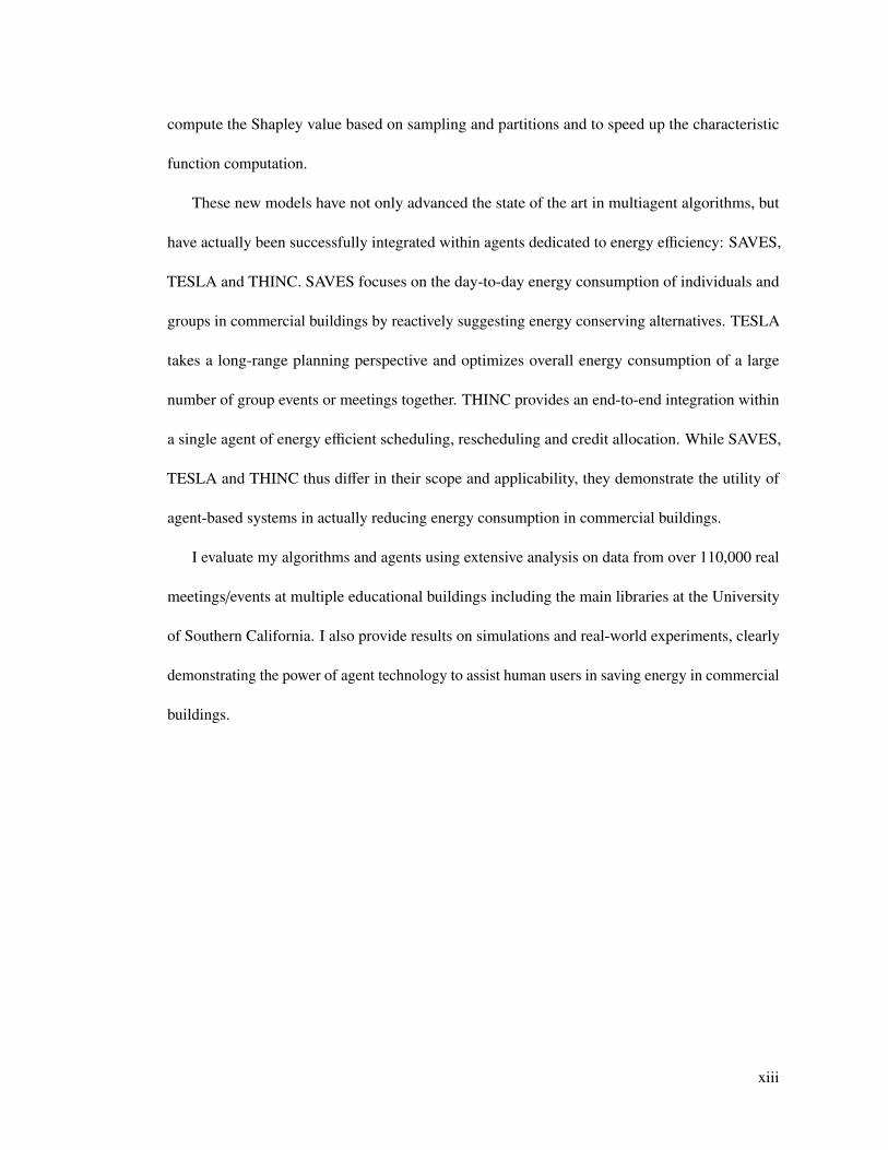
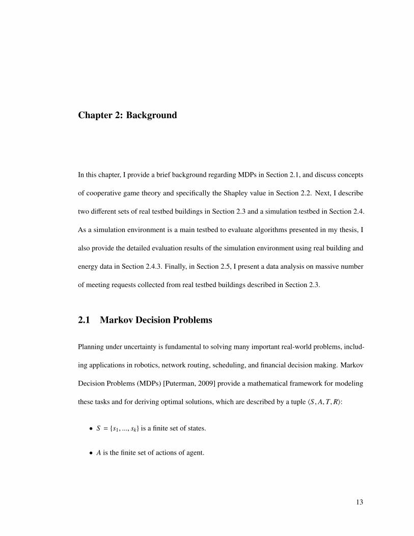
(a) The actual testbed at USC for SAVES (b) The actual testbed buildings at USC and SMU for TESLA/THINC

Figure 2.1: Real Testbed Buildings(i.e., Pi(O) = {O(1), ...,O(k − 1)}, if i = O(k)). Thus, the Shapley value can be expressed in the

following way:

φi(N, v) =∑

O∈π(N)

1n!

(v(Pi(O) ∪ i) − v(Pi(O))), i = 1, . . . , n.

2.3 Educational Building Testbeds

Recall that my work focuses on two sets of agent-based systems: SAVES and TESLA.

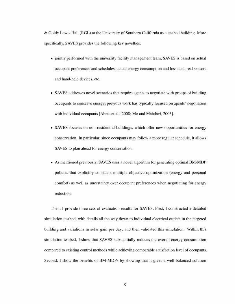
2.3.1 The actual testbed building for SAVES

SAVES, focusing on multi-objective optimization under model uncertainty, is to be deployed in

an actual educational building (Ralph & Goldy Lewis Hall (RGL)) at the University of Southern

California (shown in Figure 2.1(a)). It is a multi-functional building that has been designed with a

building management system, and it provides a good environment to test various control strategies

to mitigate energy consumption. In particular, this campus building has three floors in total and

is composed of different types of spaces including classrooms, offices for faculty and staff, and

conference rooms for meetings. Each floor has a large number of rooms and zones (a set of

16

rooms that is controlled by specific piece of equipment) with various physical properties including

different building devices, orientation, window size, room size and lighting specifications.

Within this building, components and equipment include HVAC (Heating, Ventilating, and

Air Conditioning) systems, lighting systems, office electronic devices such as computers and AV

equipment, and different types of sensors and energy meters. Human occupants of the building

are divided into two main categories: permanent and temporary. Permanent occupants include

office users such as faculty, staff, researchers and laboratory residents. Temporary occupants

include scheduled occupants like students or faculty attending classes or meetings and unscheduled

occupants who are students or faculty using common lounges or dining spaces.

In this domain, there are two types of energy-related occupant behaviors that SAVES can

influence to conserve energy use: individual behaviors and group behaviors. Individual behaviors

only affect an environment where the individual is located. They include adjusting light sources

and temperature in individual offices and turning on/off computers and other electronics. Group

behaviors lead to changes in shared spaces and require negotiation with a group of occupants in

the building. For instance, SAVES may negotiate with a group of occupants to adjust the lighting

level and temperature in their shared office or to relocate a meeting to a smaller office. As I will

show later, energy savings by considering such group negotiations together are significant.

The desired goal in this educational building is to optimize multiple criteria, i.e., achieve

maximum energy savings without trading off the comfort level of occupants. The research on this

testbed building is intended to be generalized to other building types, where we can observe many

different types of energy-use and the behavioral patterns of occupants in the buildings.

17

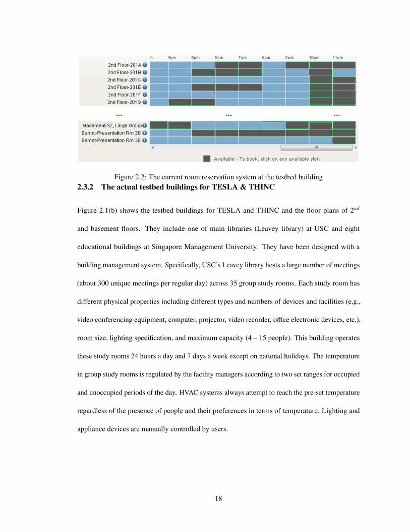
Figure 2.2: The current room reservation system at the testbed building2.3.2 The actual testbed buildings for TESLA & THINC

Figure 2.1(b) shows the testbed buildings for TESLA and THINC and the floor plans of 2nd

and basement floors. They include one of main libraries (Leavey library) at USC and eight

educational buildings at Singapore Management University. They have been designed with a

building management system. Specifically, USC’s Leavey library hosts a large number of meetings

(about 300 unique meetings per regular day) across 35 group study rooms. Each study room has

different physical properties including different types and numbers of devices and facilities (e.g.,

video conferencing equipment, computer, projector, video recorder, office electronic devices, etc.),

room size, lighting specification, and maximum capacity (4 – 15 people). This building operates

these study rooms 24 hours a day and 7 days a week except on national holidays. The temperature

in group study rooms is regulated by the facility managers according to two set ranges for occupied

and unoccupied periods of the day. HVAC systems always attempt to reach the pre-set temperature

regardless of the presence of people and their preferences in terms of temperature. Lighting and

appliance devices are manually controlled by users.

18

(a) (b)

Figure 2.3: Screen Capture of the Simulation TestbedIn this building, meetings are requested by users by a centralized online room reservation

system (see Figure 2.2). In the current reservation system, no underlying intelligent system is

used; instead, users reactively make a request based on the availability of room and time when they

access the system. While users make a request using the system, they are asked about additional

information including the number of meeting attendees and special requirements. Reservations

can be made up to 7 days in advance.

2.4 Simulation Testbed

As an important first step in deploying my work in the actual building described in the previous

section, I test my agent-based systems in a realistic simulation environment using real building

data. To that end, I have constructed a simulation testbed based on the open-source project

OpenSteer (http://opensteer.sourceforge.net/), which provides a 2D, OpenGL environment, as

shown in Figure 2.3. It can be used for efficient statistical analysis of different control strategies in

buildings before deploying the system.

19

2.4.1 Building Components

My simulation considers three building component categories: HVAC devices, lighting devices,

and appliances. The HVAC components control the temperature of the assigned zone. The lighting

devices control the lighting level of the room. The appliances in my simulation are either desktop

or laptop computers. These components have two possible actions: “on” and “standby”. When the

lighting or appliance devices are on, they consume a fixed amount of energy. My work attempts to

accurately reflect the energy consumed by each of the three component categories in the simulation.

The energy consumption of HVACs is calculated based on changes in air temperature and airflow

speeds, and gains from natural light source and appliances in the space. To calculate the energy

consumption of the lighting and appliance devices, I collected actual energy consumption data in

the testbed building. For the appliances, a desktop computer spends 0.150 kW/h and 0.010 kW/h

when it is on and standby, respectively. A laptop computer spends 0.050 kW/h when it is on and

0.005 kW/h when it is on standby.

In the simulation testbed, the energy consumption (Qz) of HVAC is calculated as follow-

ing [Standard, 2001] mainly based on changes in air temperature and airflow speeds, and gains

from natural light source and appliances in the space, etc.:

20

Qz = Qcw + Q f an, (2.5)

Qcw = 0.21 × Qcs, (2.6)

Qcs = 1.1 × (Tma − Tsa) × Vsa, (2.7)

Tma = (Vbz

Vsa) × Tosa + (1 − (

Vbz

Vsa)) × Tz, (2.8)

Q f an = 1.25 × 3.412 × Vsa, (2.9)

Vsa =(Wsa × HCda × H × A) × ∆T + Qzs

1.1 × (Tz − Tsa), (2.10)

Vbz = max(20P, 0.05A), (2.11)

Qzs = (P × 255) + (C × 500) + (LW × 3.412) + (0.5 × Azw × (Tosa − Tz)) + (S G × Azw),

(2.12)

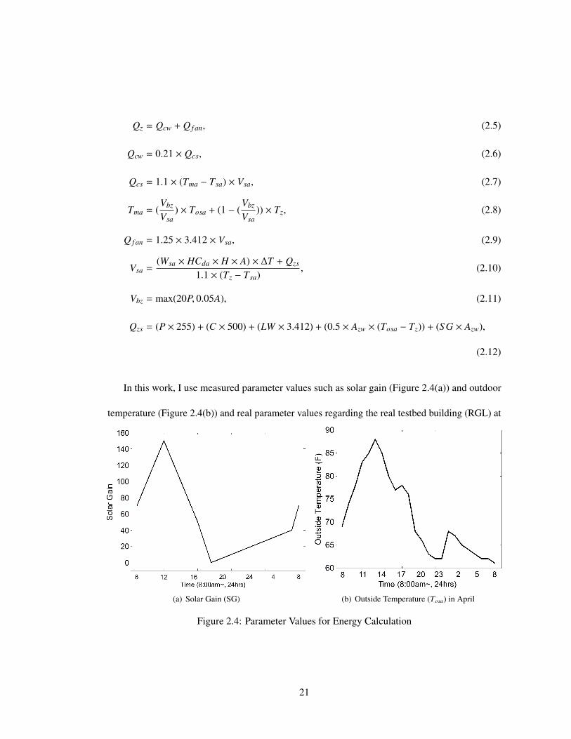
In this work, I use measured parameter values such as solar gain (Figure 2.4(a)) and outdoor

temperature (Figure 2.4(b)) and real parameter values regarding the real testbed building (RGL) at

(a) Solar Gain (SG) (b) Outside Temperature (Tosa) in April

Figure 2.4: Parameter Values for Energy Calculation

21

Table 2.1: Parameter Description for Energy Calculation

Parameters Meaning Default Value

A Zone Area (sq. ft)Azw Window Area per Zone (sq. ft)P Number of People in ZoneC Number of Computers in Current UseLW Zone Light in Current Use (Watt)Tz Desired Temperature (◦F)Tsa Temperature of Supply Air (◦F) 60.0◦FTosa Temperature of Outside AirS G Solar GainWsa Specific Weight of Air (lb/ft3) 0.07495 lb/ft3

HCda Heat Capacity Dry Air (BTU/lbF) 0.24 BTU/lbFH Ceiling Height (ft) 10.0 ft∆T Temperature change (◦F/hr)

Figure 2.5: RGL Floor Plan (2nd & 3rd floors of the testbed building)the University of Southern California (Figure 2.5) obtained from the facility management system.

Specifically, Tables 2.1 & 2.2 show the parameter values I used for the above energy calculation.

22

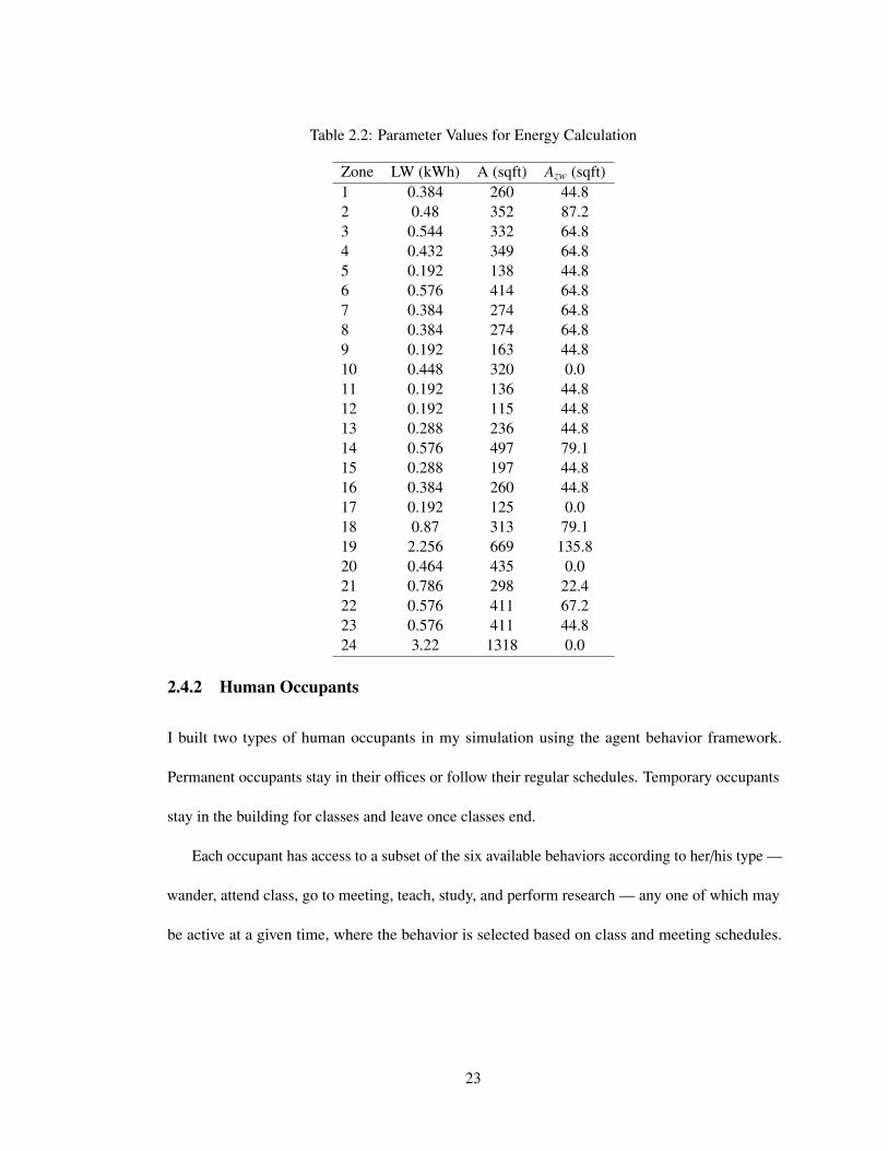
Table 2.2: Parameter Values for Energy Calculation

Zone LW (kWh) A (sqft) Azw (sqft)1 0.384 260 44.82 0.48 352 87.23 0.544 332 64.84 0.432 349 64.85 0.192 138 44.86 0.576 414 64.87 0.384 274 64.88 0.384 274 64.89 0.192 163 44.810 0.448 320 0.011 0.192 136 44.812 0.192 115 44.813 0.288 236 44.814 0.576 497 79.115 0.288 197 44.816 0.384 260 44.817 0.192 125 0.018 0.87 313 79.119 2.256 669 135.820 0.464 435 0.021 0.786 298 22.422 0.576 411 67.223 0.576 411 44.824 3.22 1318 0.0

2.4.2 Human Occupants

I built two types of human occupants in my simulation using the agent behavior framework.

Permanent occupants stay in their offices or follow their regular schedules. Temporary occupants

stay in the building for classes and leave once classes end.

Each occupant has access to a subset of the six available behaviors according to her/his type —

wander, attend class, go to meeting, teach, study, and perform research — any one of which may

be active at a given time, where the behavior is selected based on class and meeting schedules.

23

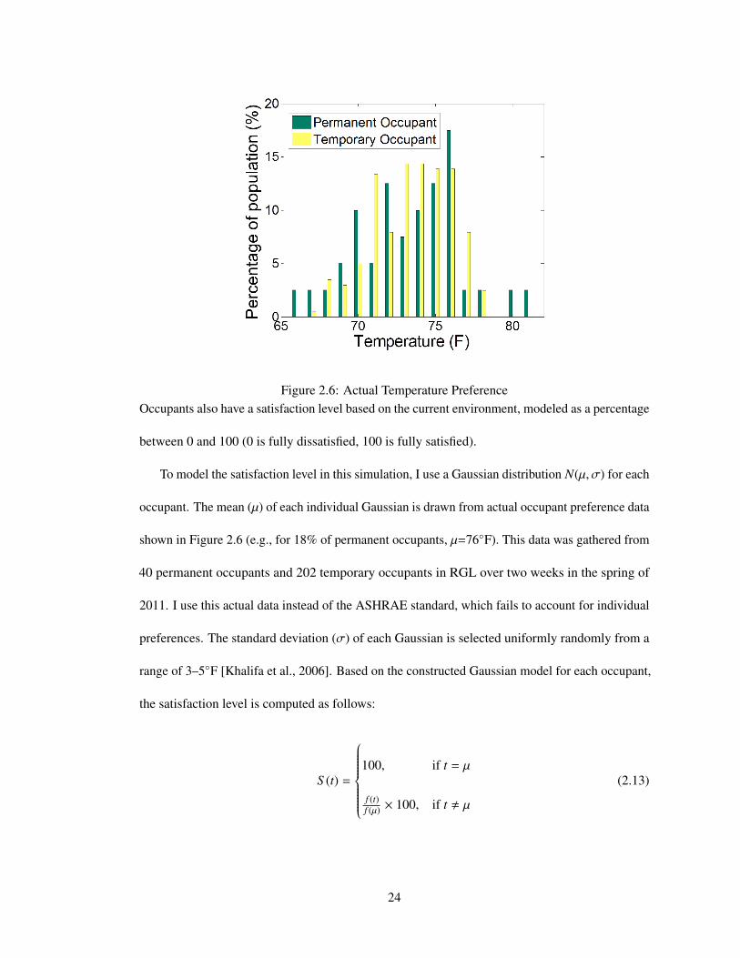
Figure 2.6: Actual Temperature PreferenceOccupants also have a satisfaction level based on the current environment, modeled as a percentage

between 0 and 100 (0 is fully dissatisfied, 100 is fully satisfied).

To model the satisfaction level in this simulation, I use a Gaussian distribution N(µ, σ) for each

occupant. The mean (µ) of each individual Gaussian is drawn from actual occupant preference data

shown in Figure 2.6 (e.g., for 18% of permanent occupants, µ=76◦F). This data was gathered from

40 permanent occupants and 202 temporary occupants in RGL over two weeks in the spring of

2011. I use this actual data instead of the ASHRAE standard, which fails to account for individual

preferences. The standard deviation (σ) of each Gaussian is selected uniformly randomly from a

range of 3–5◦F [Khalifa et al., 2006]. Based on the constructed Gaussian model for each occupant,

the satisfaction level is computed as follows:

S (t) =

100, if t = µ

f (t)f (µ) × 100, if t , µ

(2.13)

24

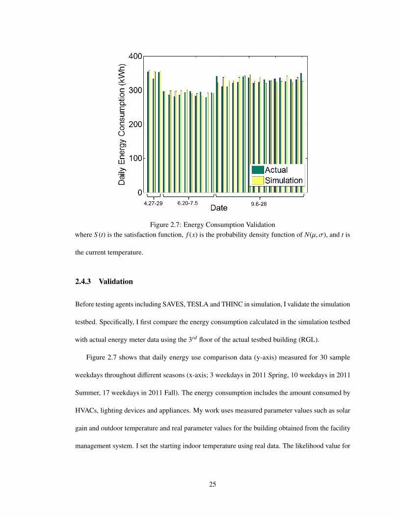
Figure 2.7: Energy Consumption Validationwhere S (t) is the satisfaction function, f (x) is the probability density function of N(µ, σ), and t is

the current temperature.

2.4.3 Validation

Before testing agents including SAVES, TESLA and THINC in simulation, I validate the simulation

testbed. Specifically, I first compare the energy consumption calculated in the simulation testbed

with actual energy meter data using the 3rd floor of the actual testbed building (RGL).

Figure 2.7 shows that daily energy use comparison data (y-axis) measured for 30 sample

weekdays throughout different seasons (x-axis; 3 weekdays in 2011 Spring, 10 weekdays in 2011

Summer, 17 weekdays in 2011 Fall). The energy consumption includes the amount consumed by

HVACs, lighting devices and appliances. My work uses measured parameter values such as solar

gain and outdoor temperature and real parameter values for the building obtained from the facility

management system. I set the starting indoor temperature using real data. The likelihood value for

25

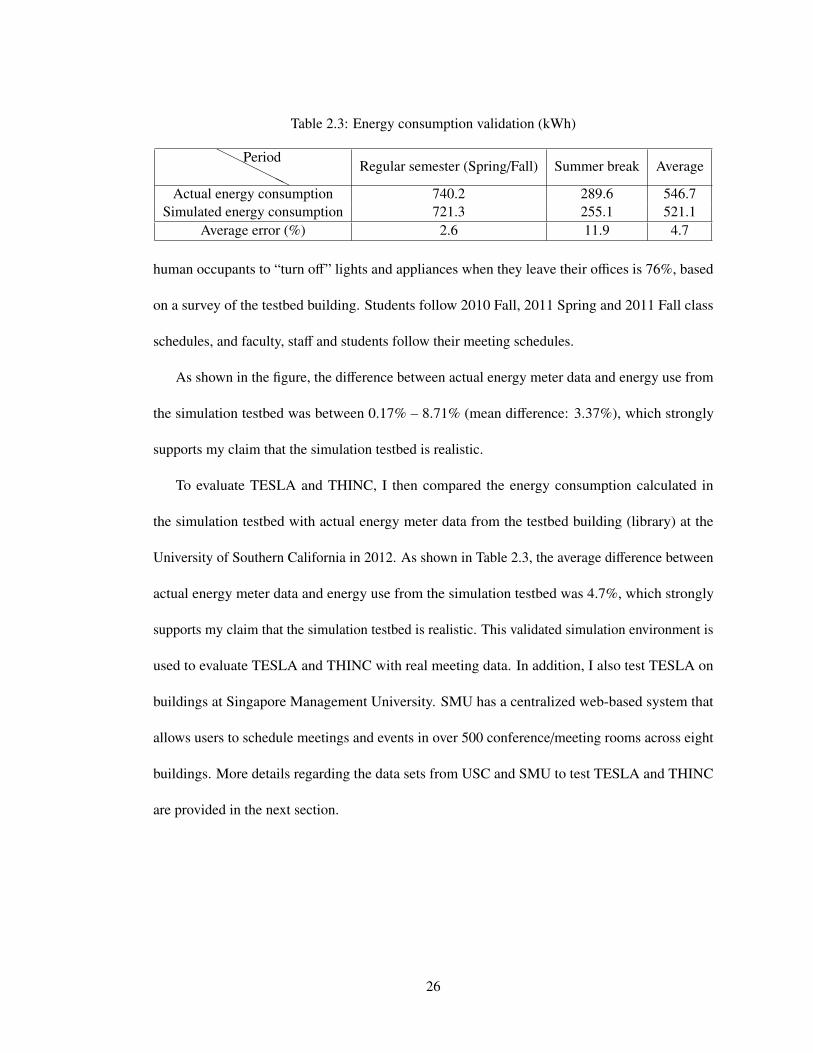
Table 2.3: Energy consumption validation (kWh)

HHHH

HH

PeriodRegular semester (Spring/Fall) Summer break Average

Actual energy consumption 740.2 289.6 546.7Simulated energy consumption 721.3 255.1 521.1

Average error (%) 2.6 11.9 4.7

human occupants to “turn off” lights and appliances when they leave their offices is 76%, based

on a survey of the testbed building. Students follow 2010 Fall, 2011 Spring and 2011 Fall class

schedules, and faculty, staff and students follow their meeting schedules.

As shown in the figure, the difference between actual energy meter data and energy use from

the simulation testbed was between 0.17% – 8.71% (mean difference: 3.37%), which strongly

supports my claim that the simulation testbed is realistic.

To evaluate TESLA and THINC, I then compared the energy consumption calculated in

the simulation testbed with actual energy meter data from the testbed building (library) at the

University of Southern California in 2012. As shown in Table 2.3, the average difference between

actual energy meter data and energy use from the simulation testbed was 4.7%, which strongly

supports my claim that the simulation testbed is realistic. This validated simulation environment is

used to evaluate TESLA and THINC with real meeting data. In addition, I also test TESLA on

buildings at Singapore Management University. SMU has a centralized web-based system that

allows users to schedule meetings and events in over 500 conference/meeting rooms across eight

buildings. More details regarding the data sets from USC and SMU to test TESLA and THINC

are provided in the next section.

26

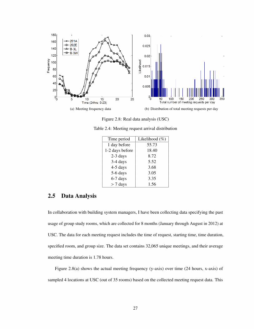
(a) Meeting frequency data (b) Distribution of total meeting requests per day

Figure 2.8: Real data analysis (USC)

Table 2.4: Meeting request arrival distribution

Time period Likelihood (%)1 day before 55.73

1-2 days before 18.402-3 days 8.723-4 days 5.524-5 days 3.685-6 days 3.056-7 days 3.35> 7 days 1.56

2.5 Data Analysis

In collaboration with building system managers, I have been collecting data specifying the past

usage of group study rooms, which are collected for 8 months (January through August in 2012) at

USC. The data for each meeting request includes the time of request, starting time, time duration,

specified room, and group size. The data set contains 32,065 unique meetings, and their average

meeting time duration is 1.78 hours.

Figure 2.8(a) shows the actual meeting frequency (y-axis) over time (24 hours, x-axis) of

sampled 4 locations at USC (out of 35 rooms) based on the collected meeting request data. This

27

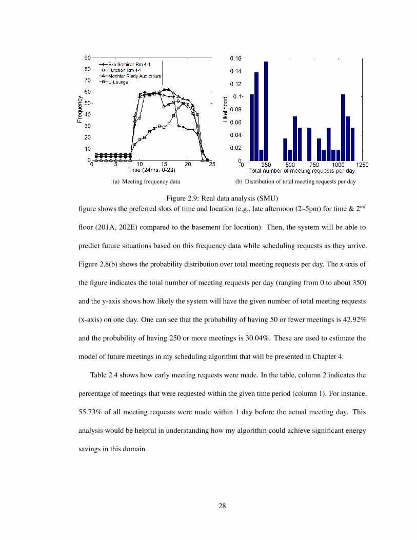
(a) Meeting frequency data (b) Distribution of total meeting requests per day

Figure 2.9: Real data analysis (SMU)figure shows the preferred slots of time and location (e.g., late afternoon (2–5pm) for time & 2nd

floor (201A, 202E) compared to the basement for location). Then, the system will be able to

predict future situations based on this frequency data while scheduling requests as they arrive.

Figure 2.8(b) shows the probability distribution over total meeting requests per day. The x-axis of

the figure indicates the total number of meeting requests per day (ranging from 0 to about 350)

and the y-axis shows how likely the system will have the given number of total meeting requests

(x-axis) on one day. One can see that the probability of having 50 or fewer meetings is 42.92%

and the probability of having 250 or more meetings is 30.04%. These are used to estimate the

model of future meetings in my scheduling algorithm that will be presented in Chapter 4.

Table 2.4 shows how early meeting requests were made. In the table, column 2 indicates the

percentage of meetings that were requested within the given time period (column 1). For instance,

55.73% of all meeting requests were made within 1 day before the actual meeting day. This

analysis would be helpful in understanding how my algorithm could achieve significant energy

savings in this domain.

28

While evaluating my work, I also consider another data set from SMU. The data set contains

over 80,000 meetings that have been collected for three months (August through October) in

2011 at SMU, which gives a sense regarding how my algorithm will handle energy-oriented

scheduling problems in large buildings. Similar to Figure 2.8, Figure 2.9(a) shows the actual

meeting frequency (y-axis) over time (24 hours, x-axis) of sampled 4 locations at SMU (out of

over 500 rooms) based on the collected meeting request data. This figure shows the preferred slots

of time and location. Figure 2.9(b) shows the probability distribution over total meeting requests

per day. The x-axis of the figure indicates the total number of meeting requests per day (ranging

from 0 to about 1200) and the y-axis shows how likely the system will have the given number of

total meeting requests (x-axis) on one day.

29

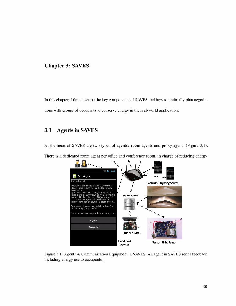
Chapter 3: SAVES

In this chapter, I first describe the key components of SAVES and how to optimally plan negotia-

tions with groups of occupants to conserve energy in the real-world application.

3.1 Agents in SAVES

At the heart of SAVES are two types of agents: room agents and proxy agents (Figure 3.1).

There is a dedicated room agent per office and conference room, in charge of reducing energy

Figure 3.1: Agents & Communication Equipment in SAVES. An agent in SAVES sends feedbackincluding energy use to occupants.

30

consumption in that room. It can access sensors to retrieve information such as the current lighting

level and temperature and energy use at different levels (building-level, floor-level, zone-level, and

room-level) and impact the operation of actuators. A proxy agent [Scerri et al., 2002] is on an

individual occupant’s hand-held device and it has the corresponding occupant’s preference and

behavior models. Proxy agents communicate on behalf of an occupant to the room agent. Such

proxy agents’ adjustable autonomy – when to interrupt a user and when to act autonomously – is

recognized as a major research issue [Scerri et al., 2002; Schurr et al., 2009], but since it is not my

focus, I use preset rules instead. Room agents may directly communicate with occupants without

proxy agents if needed. Finally, different room agents coordinate among themselves via proxy

agents, e.g., if two separate conference room agents wish to move a meeting to one occupant’s

office, the proxy of that occupant allows one of the room agents to proceed, blocking the other’s

request (see Figure 3.1).

Room agent reasoning is based on a new model called Bounded parameter Multi-objective

MDPs (BM-MDPs), which is one of the contributions of this research. BM-MDPs are a hybrid

of MO-MDPs [Chatterjee et al., 2006; Ogryczak et al., 2011] and BMDPs [Givan et al., 2000].

BM-MDPs are responsible for planning simple and complex tasks. Simple tasks include turning on

the HVAC before a class or a meeting, and do not need the full power of the BM-MDPs. Complex

tasks were why BM-MDPs were created; these include negotiating with groups of individuals

to relocate meetings to smaller rooms to save energy, negotiating with multiple occupants of a

shared office to reduce energy usage in the form of lights or HVACs, and others. Before describing

BM-MDPs in depth, I motivate their use by elaborating on the meeting relocation negotiation

scenario.

31

Group Meeting Relocation Negotiation Example Consider a meeting that has been scheduled

with two attendees (P1 and P2) in a large conference room that has more light sources and

appliances than smaller offices. Since the meeting has few attendees, the room agent can negotiate

with attendees to relocate the meeting to nearby small, sunlit offices, which can lead to significant

energy savings. The room agent handles this negotiation based on BM-MDPs. There are three

objectives (i.e., three separate reward functions) that the room agent needs to consider during this

negotiation: (i) energy saving (R1), (ii) P1’s comfort level change (R2), and (iii) P2’s comfort level

change (R3). The room agent first checks the available offices. Assuming there are two available

offices A and B, the room agent asks each attendee if she or he will agree to relocate the meeting

to one of the available offices. In asking an attendee, the room agent must consider the uncertainty

of whether an attendee is likely to accept its offer to relocate the meeting. Since asking incurs

a cost (e.g., cost caused by interrupting people), the room agent needs to reason about which

option is preferable considering P1 and P2’s likelihood to accept each option (A or B) and the

reward functions for each option to reduce the required cost and maximize benefits. Assuming

A is preferable, the optimal policy of the agent is “ask P1 first about A”–“if P1 accepts, ask P2

about A”–“if P1 does not reply, ask P1 about A again”–“repeat the process with B”–“if both agree,

relocate the meeting”–“if both disagree, find other available options.” While this is a simplified

example, in practice the problem is more difficult, as there may be more than two attendees in a

meeting. The room agent must also first communicate with the proxies of the owners of offices A

and B and there may be uncertainty in their agreement to have a meeting in their office; further

adding to the challenge of sequential decision making under uncertainty. In addition, the agent

must decide if it should ask P1 first and use that result to influence P2, etc.

32

Thus, BM-MDPs must reason with multiple objectives, but simultaneously must reason with

the uncertainty in the domain. In fact, in a complex domain such as mine, the probabilities of

attendees’ or others’ acceptance of the room agent’s offer, or the probabilities of other outcomes

may not be precisely known — we may only have a reasonable upper and lower bound over such

probabilities. Indeed, precisely knowing the model is very challenging, and I ended up building

BM-MDPs to address both these challenges and requirements. However, before explaining

BM-MDPs, I first explain MO-MDPs on which BM-MDPs are built.

3.2 Multi-objective MDPs

The negotiation scenarios described earlier require SAVES to consider multiple objectives simul-

taneously: energy consumption and satisfaction level of multiple individuals. To handle such

multiple objectives, MDPs have been extended to take into account multiple criteria assuming

no model uncertainty. Multi-Objective MDPs (MO-MDPs) [Chatterjee et al., 2006; Ogryczak

et al., 2011] are defined as an MDP where the reward function has been replaced by a vector of

rewards. Specifically, MO-MDPs are described by a tuple 〈S , A,T, {Ri}, p〉, where Ri is the reward

function for objective i and p denotes the starting state distribution (p(s) ≥ 0). In the meeting

relocation example shown in Section 3.1, specifically, the multiple reward functions, {Ri}, include

energy consumption (which is the reduction in energy usage in moving from a conference room to

a smaller office), and comfort level defined separately for each individual (based on data related to

their temperature comfort zones).

The key takeaway from MO-MDPs towards BM-MDPs is an understanding of how to generate

a policy in the presence of such multiple objectives that are not aggregated into one single value.

33

The key principle I rely on, given the current domain of non-residential buildings is one of fairness;

we wish to reduce energy usage, but we cannot sacrifice any one individual’s comfort entirely in

service of this goal. To meet this requirement, I focus on minimizing the maximum regret instead

of maximizing the reward value based on a min-max optimization technique [Osyczka, 1978] to

get a well-balanced solution.

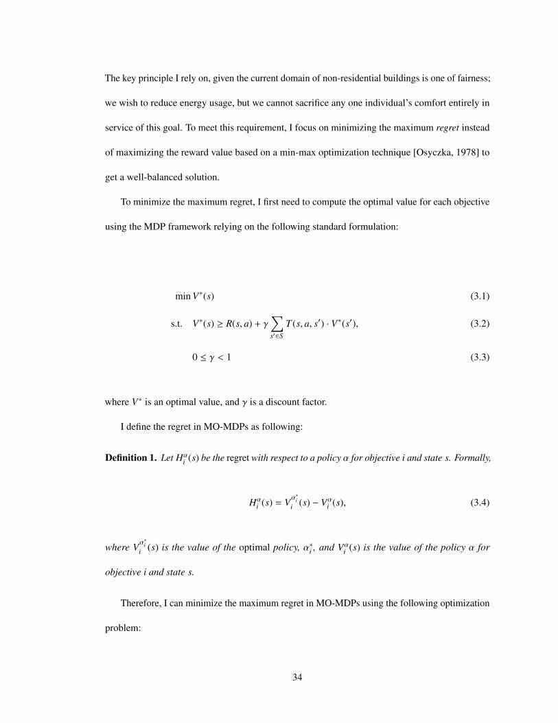
To minimize the maximum regret, I first need to compute the optimal value for each objective

using the MDP framework relying on the following standard formulation:

min V∗(s) (3.1)

s.t. V∗(s) ≥ R(s, a) + γ∑s′∈S

T (s, a, s′) · V∗(s′), (3.2)

0 ≤ γ < 1 (3.3)

where V∗ is an optimal value, and γ is a discount factor.

I define the regret in MO-MDPs as following:

Definition 1. Let Hαi (s) be the regret with respect to a policy α for objective i and state s. Formally,

Hαi (s) = V

α∗ii (s) − Vα

i (s), (3.4)

where Vα∗ii (s) is the value of the optimal policy, α∗i , and Vα

i (s) is the value of the policy α for

objective i and state s.

Therefore, I can minimize the maximum regret in MO-MDPs using the following optimization

problem:

34

min D (3.5)

s.t. D ≥∑s∈S

p(s) ·[V∗i (s) − Vi(s)

],∀i ∈ I, (3.6)

Vi(s) =∑a∈A

α(s, a)

Ri(s, a) + γ∑s′∈S

T (s, a, s′) · Vi(s′)

, (3.7)

∑a∈A

α(s, a) = 1,∀s ∈ S , 0 ≤ γ < 1 (3.8)

where V∗i is the constant value pre-calculated by (2) of the MDP formulation using the reward

function for objective i, Ri, and I is a set of objectives.

Unfortunately, in BM-MDPs, I have an upper and lower bound on transition probabilities and

rewards, and thus this optimization problem cannot be directly used. Nonetheless, it helps us

understand the key difference in minimizing max regret between MO-MDPs and BM-MDPs —

specifically in addressing such upper and lower bounds in BM-MDPs, we end up with different

transition probabilities Ti for each objective i, as discussed below, and hence rely on a different

approach to compute regret.

3.3 BM-MDPs

I now extend MO-MDPs, using ideas from BMDPs [Givan et al., 2000], to create BM-MDPs.

BMDP (represented by tuple 〈S , A, T , R, p〉) is an extension to the standard MDP, where upper

and lower bounds on transition probabilities and rewards are provided as closed real intervals. In

addition to representation of uncertainty over transition probabilities and rewards, a key takeaway

for BM-MDPs from BMDPs is the algorithm to generate policies. This algorithm is based on the

35

notion of Order-Maximizing MDPs [Givan et al., 2000], which selects transition probabilities from

the given intervals. Order-maximizing MDPs crucially take the order of states as an input – this

order is ascending for a pessimistic policy (based on lower bound values), and it is descending

for an optimistic policy (based on upper bound values). More specifically, using this order as an

input, order-maximizing MDPs construct the transition function, and generate a policy as an output

relying on value iteration. I rely on order-maximizing MDPs to generate policies in BM-MDPs as

well (but manipulate the order of states input). To provide some intuition behind the operations

of the order-maximizing MDPs, I provide a simple example to show how transition values are

assigned from their intervals using the given order in the following example. For more details,

please refer to [Givan et al., 2000].

Example of Order Maximizing MDPs Consider a BMDP with two states: s1 and s2. The

transition ranges are T (s1, a, s1) = [0.5, 0.9], T (s1, a, s2) = [0.2, 0.6]. Let us assume that the upper

bound of value is Vub(s1) = 3 and Vub(s2) = 2 at a certain iteration of order-maximizing MDP value

iteration. In BMDP, the intuition is that for calculating the optimistic value, it requires movement

to s1 as much as possible within the given range of transition probability (since it has a higher

upper bound value). Therefore to create an optimistic policy, the input to the order-maximizing

MDPs is to sort the states in a descending order based on the upper bounds. Given this input, the

transition probabilities in the order-maximizing MDP for calculating optimistic value would be

T ′(s1, a, s1) = 0.8 because T ′(s1, a, s2) should be at least 0.2, and T ′(s1, a, s2) = (1 - 0.8). Based

on these transition probabilities, I obtain a new set of expected values via value iteration, generate

a new descending order, and iterate until convergence.

36

Similar to BMDPs, the transition and reward functions in BM-MDPs have closed real intervals.

Whereas BMDPs are limited to optimizing a single objective case (i.e., the BMDP model requires

one unified reward function), BM-MDPs can (i) optimize over multiple objectives (i.e., a vector of

reward functions) with (ii) different degrees of model uncertainty. Specifically, BM-MDPs are

described by a tuple 〈S , A, T , {Ri}, p〉, where Ri represents the reward function for objective i.

Algorithm 1 SolveBMMDP()1: for i = 1 ∈ I do2:

⟨V∗i,lb,V

∗i,ub

⟩← SolveBMDP(BMDPi)

3: {V′

i,lb} ← ∞ ; {Vi,lb} ← 04: while |{V′i,lb} − {Vi,lb}| > ε do5: {Vi,lb} ← {V

′

i,lb}

6: for i = 1 ∈ I do7: Oi ← SortIncreasingOrder({Vi,lb})8: Mi ← ConstructOrderMaximizingMDP(Oi);9: {V′i,lb} ← SolveMOMDPPessimistic({Vi,lb}, {V∗i,lb}, {Mi})

10: αpes ← ObtainPessimisticPolicy({Vi,lb})11: {V

′

i,ub} ← ∞ ; {Vi,ub} ← 012: while |{V′i,ub} − {Vi,ub}| > ε do13: {Vi,ub} ← {V′i,ub}

14: for i = 1 ∈ I do15: Oi ← SortDecreasingOrder({Vi,ub})16: Mi ← ConstructOrderMaximizingMDP(Oi);17: {V′i,ub} ← SolveMOMDPOptimistic({Vi,ub}, {V∗i,ub}, {Mi})18: αopt ← ObtainOptimisticPolicy({Vi,ub})19: return {

⟨αpes, αopt

⟩}

To solve BM-MDPs, I introduce a novel algorithm that is a hybrid of BMDPs and MO-MDPs.

Specifically, my algorithm marries the minimization of max regret idea from MO-MDPs with

that of order maximizing MDPs to handle uncertainty over transition function and rewards. The

overall flow is described in Algorithm 1. At a higher level, there are three stages: (i) computing

the optimal value bounds⟨V∗i,lb,V

∗i,ub

⟩for each objective i using BMDPs (lines 1–2), (ii) using

the MO-MDP idea to optimize multiple objectives based on a min-max formulation (lines 3–9 &

11–17), and (iii) obtaining a policy α based on the final value functions⟨{Vi,lb}, {Vi,ub}

⟩(lines 10

37

& 18). The output of this algorithm is in the form of two policies (pessimistic and optimistic), and

I leave it to the user to determine which one is used.

I now describe the computation of the pessimistic policy (lines 3–10). The optimistic policy

(lines 11–18) is similarly computed. The pessimistic policy minimizes the maximum regret with

respect to the optimal lower bound values of all objectives ({V∗i,lb}) over all states; this computation

is iteratively performed in line 9. For each objective i, I first get an ascending order of states using

the current lower bound values Vi,lb (line 7) to construct the order-maximizing MDP (line 8). This

set of order-maximizing MDPs, {Mi}, is an input to the function SolveMOMDPPessimistic() to

optimize multiple objectives by directly computing regret on line 9. This computation is performed

by Eq. (3.5) with a different transition probability function Ti in the given Mi instead of T . This

in turn influences the sorting order of states, and the process continues until the expected values

{Vi,lb} converge.

3.4 Evaluation of SAVES

In this section, I provide three sets of evaluations: two sets of results tested in the simulation

testbed and a set of results tested in the real-world.

3.4.1 Simulation: Overall Evaluation

I evaluate the performance of SAVES using both 2nd and 3rd floors of RGL in the simulation

environment. I test BM-MDPs using a pessimistic setting and compare it with two other control

heuristics discussed below.

38

Manual Control: The manual control strategy is the baseline system that represents the current

strategy operated by the facility management team in the real testbed building (RGL). In this

strategy, temperature is regulated by the facility managers according to two set ranges for occupied

(70◦F–75◦F) and unoccupied periods (50◦F–90◦F) of the day. In this control setting, HVACs

always attempt to reach the pre-set temperature regardless of the presence of occupants and their

preferences in terms of temperature. Lighting and appliance devices are controlled by human

occupants. The same likelihood value for human occupants to “turn off” lights and appliances was

used as in Section 2.4.

Reactive Control: I consider the reactive control heuristic for comparison purposes since it can

be easily implemented using cheap sensors in the real building, and recently, some buildings have

already started adopting this simple heuristic to reduce energy use. The lighting and appliance

devices are now automatically controlled and turned on and off according to the presence of

people. Additionally, as in [Jazizadeh et al., 2011], appropriate temperature set points of HVACs

are computed based on the average preference of human occupants. HVACs automatically turn on

and off according to the presence of people and temperature set points.

I focus on measuring two different criteria — total energy consumption (kWh) and average

satisfaction level of occupants (%). The experiments were run on Intel Core2 Duo 2.53GHz CPU

with 4GB main memory. All techniques were evaluated for 100 independent trials throughout this

section. I report the average values.

3.4.1.1 Result: Total Energy Consumption

I compared the cumulative total energy consumption measured during 24 hours for all control

strategies. Figure 3.2(a) shows the cumulative total energy consumption on the y-axis in kWh

39

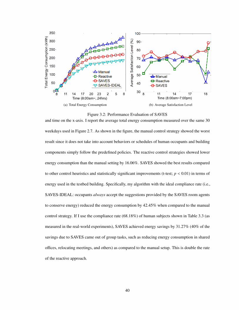
(a) Total Energy Consumption (b) Average Satisfaction Level

Figure 3.2: Performance Evaluation of SAVESand time on the x-axis. I report the average total energy consumption measured over the same 30

weekdays used in Figure 2.7. As shown in the figure, the manual control strategy showed the worst

result since it does not take into account behaviors or schedules of human occupants and building

components simply follow the predefined policies. The reactive control strategies showed lower

energy consumption than the manual setting by 16.06%. SAVES showed the best results compared

to other control heuristics and statistically significant improvements (t-test; p < 0.01) in terms of

energy used in the testbed building. Specifically, my algorithm with the ideal compliance rate (i.e.,

SAVES-IDEAL: occupants always accept the suggestions provided by the SAVES room agents

to conserve energy) reduced the energy consumption by 42.45% when compared to the manual

control strategy. If I use the compliance rate (68.18%) of human subjects shown in Table 3.3 (as

measured in the real-world experiments), SAVES achieved energy savings by 31.27% (40% of the

savings due to SAVES came out of group tasks, such as reducing energy consumption in shared

offices, relocating meetings, and others) as compared to the manual setup. This is double the rate

of the reactive approach.

40

3.4.1.2 Result: Average Satisfaction Level

Here, I compare the average satisfaction level of human occupants under different control strategies

in the simulation testbed. Figure 3.2(b) shows the average satisfaction level in percentage on

the y-axis and time on the x-axis. As shown in the results, the manual setting and my novel

algorithm showed the best results. This is because the manual setting makes HVACs attempt to

reach the desired temperature set point as soon as possible while disregarding the resulting energy

consumption, and my method plans ahead of the schedules; thus, these two can achieve the desired

comfort level faster than the reactive control strategy.

The manual strategy, however, is very sensitive to the given temperature range. In the experi-

ment, the temperature set point was set by the facility management team (e.g., 70–75◦F) based

on the average preference model, thus it achieved high comfort level in the testbed. However, if

the actual preferred temperature in the building is different from the average model, it fails to

meet the occupant’s desired level. This phenomenon can be seen when occupants stay during the

unoccupied time (after typical working hours). As can be seen at 18 on the x-axis (i.e., 6pm) in

the figure, the average comfort level drops significantly. Due to the delayed effects in temperature

change, the reactive control strategy showed significantly lower satisfaction results than other

methods. For instance, it has a satisfaction level below 60% at 14 on the x-axis (i.e., 2pm). Thus,

SAVES not only provides superior energy savings, but also avoids the reduction in comfort level

that a reactive strategy may cause.

3.4.2 Simulation: Multi-objective Optimization

In this section, I perform more analysis on my novel algorithm. Table 3.1 shows the average

maximum regret comparison tested in 5 different problem sets between the standard MDP with

41

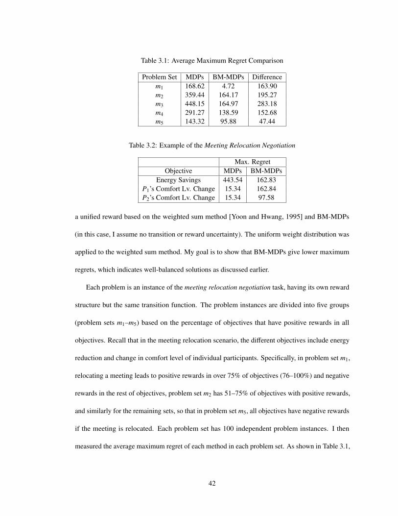
Table 3.1: Average Maximum Regret Comparison

Problem Set MDPs BM-MDPs Differencem1 168.62 4.72 163.90m2 359.44 164.17 195.27m3 448.15 164.97 283.18m4 291.27 138.59 152.68m5 143.32 95.88 47.44

Table 3.2: Example of the Meeting Relocation Negotiation

Max. RegretObjective MDPs BM-MDPs

Energy Savings 443.54 162.83P1’s Comfort Lv. Change 15.34 162.84P2’s Comfort Lv. Change 15.34 97.58

a unified reward based on the weighted sum method [Yoon and Hwang, 1995] and BM-MDPs

(in this case, I assume no transition or reward uncertainty). The uniform weight distribution was

applied to the weighted sum method. My goal is to show that BM-MDPs give lower maximum

regrets, which indicates well-balanced solutions as discussed earlier.

Each problem is an instance of the meeting relocation negotiation task, having its own reward

structure but the same transition function. The problem instances are divided into five groups

(problem sets m1–m5) based on the percentage of objectives that have positive rewards in all

objectives. Recall that in the meeting relocation scenario, the different objectives include energy

reduction and change in comfort level of individual participants. Specifically, in problem set m1,

relocating a meeting leads to positive rewards in over 75% of objectives (76–100%) and negative

rewards in the rest of objectives, problem set m2 has 51–75% of objectives with positive rewards,

and similarly for the remaining sets, so that in problem set m5, all objectives have negative rewards

if the meeting is relocated. Each problem set has 100 independent problem instances. I then

measured the average maximum regret of each method in each problem set. As shown in Table 3.1,

42

BM-MDPs always showed lower maximum regrets (column 3) compared to the MDP with uniform

weight (column 2), which suggests that my method gives well-balanced solutions regardless of

reward characteristics.

The next question is what the well-balanced solution means in energy domains. Let us take the

meeting relocation example with two attendees (P1 and P2) discussed in Section 3.1. In Table 3.2,

column 1 shows three objectives (energy savings and two attendees’ comfort level change) and

columns 2–3 indicate the maximum regret from MDPs and BM-MDPs, respectively. As shown

in the table, MDPs generated a policy that almost entirely disregards energy-savings, leading to

significantly large regrets (row 3, column 2). BM-MDPs, on the other hand, were able to achieve

small regrets over all objectives (rows 3–5, column 3).

Lastly, I test my BM-MDP algorithm considering different degrees of model uncertainty.

Figure 3.3 shows the average maximum regret tested over 100 different problem instances on the

y-axis. I choose 1 problem from each problem set (m1, m2, · · · , m5) from the previous test. The

noise of each model is proportional (20%) to the mean reward value and transition probability.

MDPs and MO-MDPs generate policies ignoring the model’s uncertainty and BM-MDPs generate

two types of policies (BM-MDP-Pes: pessimistic, BM-MDP-Opt: optimistic) that explicitly

account for the uncertainty. I then randomly generate 20 different instances within the range for

each problem (e.g., for m1, I generate m1,1, · · · , m1,20). Each generated policy is evaluated over

those 20 problem instances and the average maximum regret is computed for each algorithm.

For the other 4 problems (m2, · · · , m5), I repeat the same procedure and report the overall

average value. As shown in the figure, BM-MDPs have the best performance (i.e., lowest average

maximum regret), which means BM-MDPs are capable of generating more robust and well-

balanced solutions compared to previous work when there is model uncertainty. However, the

43

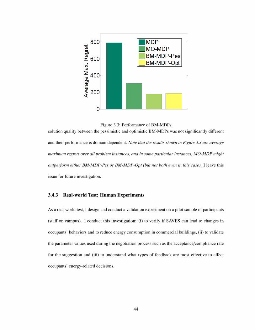
Figure 3.3: Performance of BM-MDPssolution quality between the pessimistic and optimistic BM-MDPs was not significantly different

and their performance is domain dependent. Note that the results shown in Figure 3.3 are average

maximum regrets over all problem instances, and in some particular instances, MO-MDP might

outperform either BM-MDP-Pes or BM-MDP-Opt (but not both even in this case). I leave this

issue for future investigation.

3.4.3 Real-world Test: Human Experiments

As a real-world test, I design and conduct a validation experiment on a pilot sample of participants

(staff on campus). I conduct this investigation: (i) to verify if SAVES can lead to changes in

occupants’ behaviors and to reduce energy consumption in commercial buildings, (ii) to validate

the parameter values used during the negotiation process such as the acceptance/compliance rate

for the suggestion and (iii) to understand what types of feedback are most effective to affect

occupants’ energy-related decisions.

44

In this study, I consider two test conditions: (i) feedback without motivation (Test Group I)

(e.g., please reduce the lighting level in your office), and (ii) feedback with motivation including

participant’s own energy use, and environmental motives (Test Group II) (e.g., if you reduce your

lighting for working hours, the annual energy savings at the building level are 26000kWh on

average, which is equivalent to the reduction of CO2 emissions of 2.2 homes for one year). From

this experiment, I answer the following question by comparing change in energy behavior patterns

and possible estimated energy consumption between test groups I and II.

Hypothesis 1. More informed feedback (provided to subjects in Test Group II) will be more

effective to conserve energy than feedback without motivation (Test Group I).

I tested the hypothesis above as follows: I first recruited 22 staff from 7 buildings at the

University of Southern California who are over 18 years old. Subjects were tested under two

different conditions, and each test group had 11 individuals respectively, each of whom has her/his

own office. Since I tested using a simple lighting negotiation scenario, each participant must

be able to adjust the lighting levels in her/his office. With participants’ agreements, I installed

lighting sensors (Figure 3.1) in their offices. During the experiment, participants were supposed to

stay in their own offices and do their regular work. I then measured the baseline energy behavior

and energy consumption, and SAVES provided feedback via emails based on sensed lighting

level (two times per day, at 11am and 2pm, for three consecutive weekdays). In each message,

participants received a simple suggestion for lighting level with a certain type of feedback (e.g.,

please reduce the lighting level in your office). I systematically observed and logged their energy

behavior during the entire experiment using the light sensors. At the end of the experiment, each

participant was required to take a short survey (i.e., the reasons why they agree or disagree with a

45

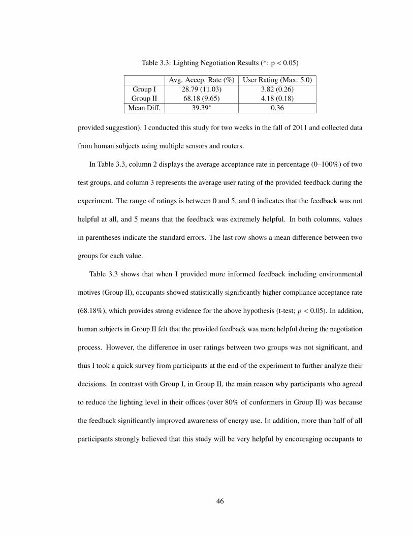
Table 3.3: Lighting Negotiation Results (*: p < 0.05)

Avg. Accep. Rate (%) User Rating (Max: 5.0)Group I 28.79 (11.03) 3.82 (0.26)Group II 68.18 (9.65) 4.18 (0.18)

Mean Diff. 39.39∗ 0.36

provided suggestion). I conducted this study for two weeks in the fall of 2011 and collected data

from human subjects using multiple sensors and routers.

In Table 3.3, column 2 displays the average acceptance rate in percentage (0–100%) of two

test groups, and column 3 represents the average user rating of the provided feedback during the

experiment. The range of ratings is between 0 and 5, and 0 indicates that the feedback was not

helpful at all, and 5 means that the feedback was extremely helpful. In both columns, values

in parentheses indicate the standard errors. The last row shows a mean difference between two

groups for each value.

Table 3.3 shows that when I provided more informed feedback including environmental

motives (Group II), occupants showed statistically significantly higher compliance acceptance rate

(68.18%), which provides strong evidence for the above hypothesis (t-test; p < 0.05). In addition,

human subjects in Group II felt that the provided feedback was more helpful during the negotiation

process. However, the difference in user ratings between two groups was not significant, and

thus I took a quick survey from participants at the end of the experiment to further analyze their

decisions. In contrast with Group I, in Group II, the main reason why participants who agreed

to reduce the lighting level in their offices (over 80% of conformers in Group II) was because

the feedback significantly improved awareness of energy use. In addition, more than half of all

participants strongly believed that this study will be very helpful by encouraging occupants to

46

think about energy usage. This discrepancy in average user ratings and acceptance rates remains

an issue for future work.

In this trial study, I have learned that although occupants in commercial buildings do not have

a direct financial incentive in saving energy, proper motivations can achieve a higher compliance

rate for the energy-related suggestion. This study specifically provides the insights that there is a

significant potential to conserve energy by investigating effective and tailored methods to improve

occupants’ motivation to conserve energy.

47

Chapter 4: TESLA

In this chapter, I describe the overall architecture of TESLA and how to optimally schedule

meetings in real-world situations to conserve energy in commercial buildings.

4.1 TESLA Architecture

TESLA is a goal-seeking (to save energy), continuously running autonomous agent. TESLA

performs on-line energy-efficient scheduling while considering dynamically arriving inputs from

Figure 4.1: TESLA architecture: TESLA is a continuously running agent that supports four keyfeatures: (i) energy-efficient scheduling; (ii) identification of key meetings; (iii) learning of userpreferences; and (iv) communication with users.

48

users; these dynamic inputs make the scheduling complex and TESLA needs to learn a predictive

model for users’ inputs and preferences (see Figure 4.1). More specifically, TESLA :

• takes inputs (i.e., preferred time, location, the number of meeting attendees, etc.) from

different users and their proxy agents at different times

• autonomously performs on-line energy-efficient scheduling as requests arrive while balanc-

ing user comfort

• autonomously, on own initiative, interacts with different users based on identified problem-

atic key meetings in order to avoid bother cost to users while persuading them to change

meeting flexibility

• bases its non-myopic optimization on learned patterns of meetings

As shown in Figure 4.1, meeting requests are the information I get from the interface of TESLA

via the web interface (or via a proxy agent [Scerri et al., 2002] on an individual user’s hand-held

device, in case the users have proxy agents, who have the corresponding users’ preferences and

behavior models with a certain level of adjustable autonomy). TESLA focuses on minimizing

unnecessary interactions by detecting a small number of key meetings while negotiating with

people to adjust their flexibility. TESLA may interact with users’ proxy agents instead of the users

themselves.

4.2 TESLA Algorithms

The objective of this work is to come up with energy efficient schedules in commercial buildings

with a large number of meetings while considering (i) flexibility in meeting requests over time,

49

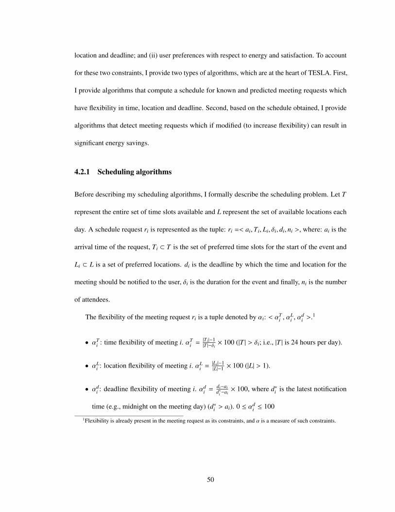
location and deadline; and (ii) user preferences with respect to energy and satisfaction. To account

for these two constraints, I provide two types of algorithms, which are at the heart of TESLA. First,

I provide algorithms that compute a schedule for known and predicted meeting requests which

have flexibility in time, location and deadline. Second, based on the schedule obtained, I provide

algorithms that detect meeting requests which if modified (to increase flexibility) can result in

significant energy savings.

4.2.1 Scheduling algorithms

Before describing my scheduling algorithms, I formally describe the scheduling problem. Let T

represent the entire set of time slots available and L represent the set of available locations each

day. A schedule request ri is represented as the tuple: ri =< ai,Ti, Li, δi, di, ni >, where: ai is the

arrival time of the request, Ti ⊂ T is the set of preferred time slots for the start of the event and

Li ⊂ L is a set of preferred locations. di is the deadline by which the time and location for the

meeting should be notified to the user, δi is the duration for the event and finally, ni is the number

of attendees.

The flexibility of the meeting request ri is a tuple denoted by αi: < αTi , αL

i , αdi >.1

• αTi : time flexibility of meeting i. αT

i =|Ti |−1|T |−δi

× 100 (|T | > δi; i.e., |T | is 24 hours per day).

• αLi : location flexibility of meeting i. αL

i =|Li |−1|L|−1 × 100 (|L| > 1).

• αdi : deadline flexibility of meeting i. αd

i =di−aid∗i −ai

× 100, where d∗i is the latest notification

time (e.g., midnight on the meeting day) (d∗i > ai). 0 ≤ αdi ≤ 100

1Flexibility is already present in the meeting request as its constraints, and α is a measure of such constraints.

50

Figure 4.2: Disjoint sets of RFor instance, given only one time slot (|Ti| = 1), αT

i = 0 and all available time slots (|Ti| =

|T | − δi + 1), αTi = 100. Assuming that people give Ti = 4–7pm on Monday and their meeting time

duration is 2 hours, then αTi = (4-1)/(24-2) × 100 = 13.64%. Likewise, given only one location

slot (|Li| = 1), αLi = 0 and given all available locations (|Li| = |L|), αT

i = 100.

I now define specific disjoint sets of meeting requests, R, that characterize different types of

scheduling algorithms, where t is the time to schedule a given set of requests R.

• RS (t) = {i : di = t and ai ≤ t}: a set of requests that have to be scheduled at time t

• RA(t) = {i : di < t and ai < t}: a set of requests that were assigned before time t

• RK(t) = {i : di > t and ai ≤ t}: a set of known future requests, which arrived before time t,

but will be scheduled in the future

• RU(t) = {i : di > t and ai > t}: a set of unknown future requests

As a simple example (shown in Figure 4.2), let us consider that we have 4 meeting requests

(r1, r2, r3, and r4), which are supposed to be scheduled on the same day. The current time is t.

According to the definition, RS (t) = {r2},RA(t) = {r1},RK(t) = {r3}, and RU(t) = {r4}.

Given a set of requests, R, I provide a two-stage stochastic mixed integer linear program

(SMILP) to compute a schedule that minimizes the overall energy consumption. Stochastic

51

programming has provided a framework for modeling optimization problems that involve un-

certainty [Beale, 1955; Dantzig, 1955; Kall and Wallace, 1994; Shapiro et al., 2009]. Whereas

deterministic optimization problems are formulated with known parameters, real world problems

almost invariably include some unknown parameters. In particular, my scheduling problem aims to

optimally schedule incrementally/dynamically arriving requests, and thus I should consider uncer-

tainty in terms of future requests, which makes deterministic optimization techniques inapplicable.

To address this challenge, I specifically formulate my scheduling problem as a two-stage stochastic

program. Here the decision variables are partitioned into two sets. The first stage variables are

decided before the actual realization of the uncertain parameters are known. Afterward, once the

random events have exhibited themselves, further decisions can be made by selecting the values

of the second stage. The second stage decision variables can be made to minimize penalties that

may occur as a result of the first stage decision. This SMILP will be run every time a new meeting

request arrives (or after a batch of meeting requests arrive in close succession).

The notation that will be employed in the SMILP is as follows:

• xil,t is the first stage binary variable that is set to 1 if meeting request ri is scheduled in

location l starting at time t.

• Eil,t is a constant that is computed for a meeting request ri if it is scheduled in location l at

time t using the HVAC energy consumption equations.

• C is a constant that indicates the reduction in energy consumption because of scheduling a

meeting in the previous time slot. Although I assumed that C is a constant for simplicity in

this work, it depends on different factors of previous meetings in practice.

52

• eil,t is a continuous variable that corresponds to the energy consumed because of scheduling

meeting i in location l at time t. The value of this variable is affected based on whether

there is a meeting scheduled in the previous time slot (t − 1), i.e., the reduction that would

occur at location l at time t if a meeting was scheduled at location l at time t − 1. 2

eil,t = xi

l,t · Eil,t −

∑i′∈R\{i} xi′

l,t−1 ·C.

• S il,t is a value that indicates the satisfaction level obtained with users in meeting request ri

for scheduling the meeting in location l at time t. B is a threshold on the satisfaction level

required by users.

• M is an arbitrarily large positive constant.

• Q(x, ξ) is the value function of future energy consumption, where ξ represents uncertainty

over the second stage problem (i.e., future meeting situations in the problem). ξ determines

a vector of parameters, (w, q).

• w jl,t is the second stage binary variable that is set to 1 if meeting request r j in a future meeting

request set is scheduled in location l starting at time t.

• q jl,t is a continuous second stage variable that corresponds to the future energy consumed

because of scheduling meeting j in location l at time t.

I first provide the SMILP and a detailed explanation of the constraints.

2eil,t gets affected by a meeting in the previous time slot in the same location. This is because adjacent meetings

affect the indoor temperature, which makes HVACs operate differently to maintain the desired temperature level.

53

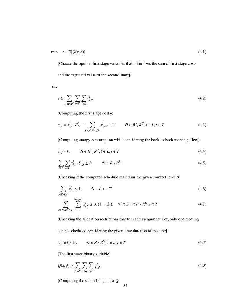
min e + E[Q(x, ξ)] (4.1)

{Choose the optimal first stage variables that minimizes the sum of first stage costs

and the expected value of the second stage}

s.t.

e ≥∑

i∈R\RU

∑t∈T

∑l∈L

eil,t, (4.2)

{Computing the first stage cost e}

eil,t = xi

l,t · Eil,t −

∑i′∈R\RU\{i}

xi′l,t−1 ·C, ∀i ∈ R \ RU , l ∈ L, t ∈ T (4.3)

{Computing energy consumption while considering the back-to-back meeting effect}

eil,t ≥ 0, ∀i ∈ R \ RU , l ∈ L, t ∈ T (4.4)∑t∈T

∑l∈L

xil,t · S

il,t ≥ B, ∀i ∈ R \ RU (4.5)

{Checking if the computed schedule maintains the given comfort level B}∑i∈R\RU

xil,t ≤ 1, ∀l ∈ L, t ∈ T (4.6)

∑i′∈R\RU\{i}

t+δi−1∑t′=t

xi′l,t′ ≤ M(1 − xi

l,t), ∀l ∈ L, i ∈ R \ RU , t ∈ T (4.7)

{Checking the allocation restrictions that for each assignment slot, only one meeting

can be scheduled considering the given time duration of meeting}

xil,t ∈ {0, 1}, ∀i ∈ R \ RU , l ∈ L, t ∈ T (4.8)

{The first stage binary variable}

Q(x, ξ) ≥∑j∈RU

∑l∈L

∑t∈T

q jl,t, (4.9)

{Computing the second stage cost Q}54

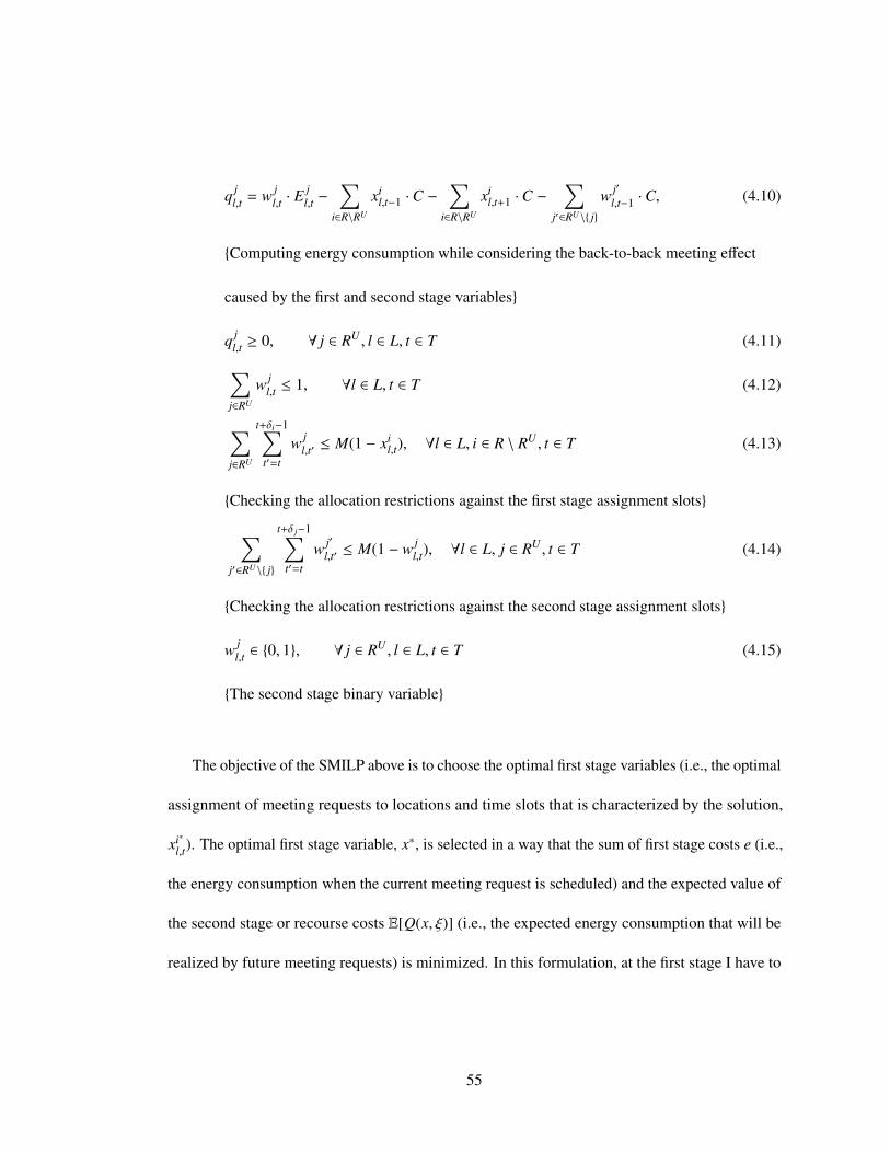
q jl,t = w j

l,t · Ejl,t −

∑i∈R\RU

xil,t−1 ·C −

∑i∈R\RU

xil,t+1 ·C −

∑j′∈RU\{ j}

w j′

l,t−1 ·C, (4.10)

{Computing energy consumption while considering the back-to-back meeting effect

caused by the first and second stage variables}

q jl,t ≥ 0, ∀ j ∈ RU , l ∈ L, t ∈ T (4.11)∑

j∈RU

w jl,t ≤ 1, ∀l ∈ L, t ∈ T (4.12)

∑j∈RU

t+δi−1∑t′=t

w jl,t′ ≤ M(1 − xi

l,t), ∀l ∈ L, i ∈ R \ RU , t ∈ T (4.13)

{Checking the allocation restrictions against the first stage assignment slots}

∑j′∈RU\{ j}

t+δ j−1∑t′=t

w j′

l,t′ ≤ M(1 − w jl,t), ∀l ∈ L, j ∈ RU , t ∈ T (4.14)

{Checking the allocation restrictions against the second stage assignment slots}

w jl,t ∈ {0, 1}, ∀ j ∈ RU , l ∈ L, t ∈ T (4.15)

{The second stage binary variable}

The objective of the SMILP above is to choose the optimal first stage variables (i.e., the optimal

assignment of meeting requests to locations and time slots that is characterized by the solution,

xi∗l,t). The optimal first stage variable, x∗, is selected in a way that the sum of first stage costs e (i.e.,

the energy consumption when the current meeting request is scheduled) and the expected value of

the second stage or recourse costs E[Q(x, ξ)] (i.e., the expected energy consumption that will be

realized by future meeting requests) is minimized. In this formulation, at the first stage I have to

55

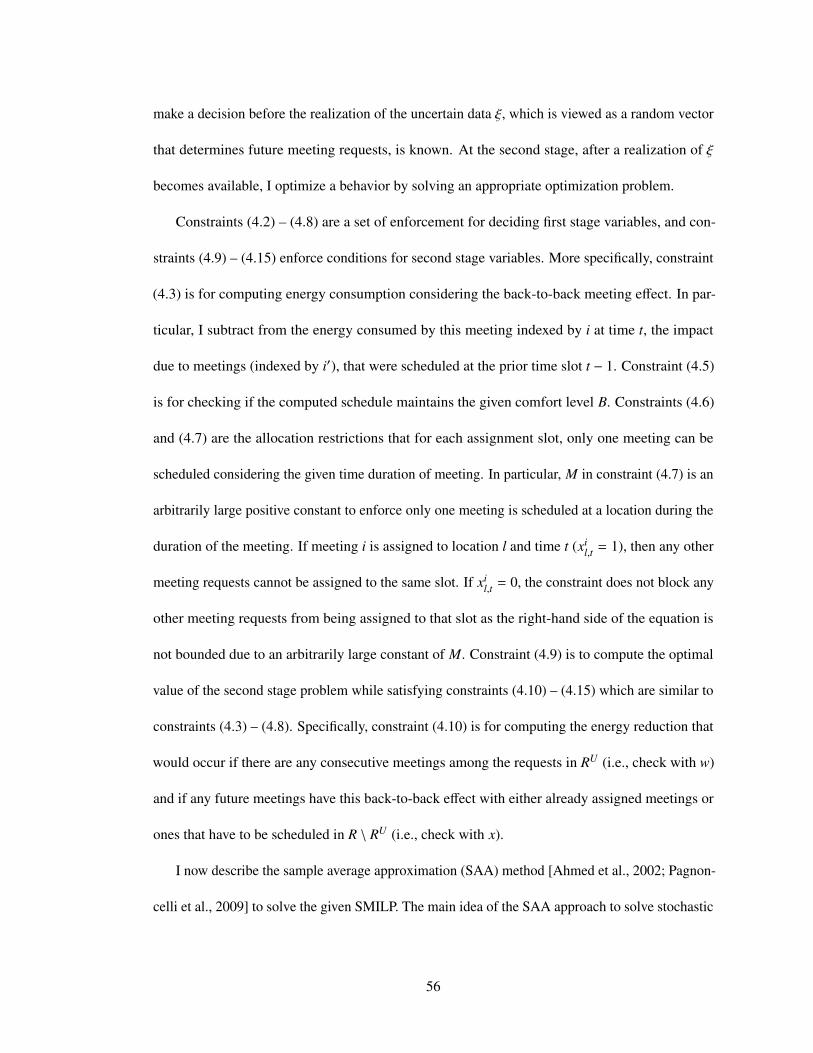
make a decision before the realization of the uncertain data ξ, which is viewed as a random vector

that determines future meeting requests, is known. At the second stage, after a realization of ξ

becomes available, I optimize a behavior by solving an appropriate optimization problem.

Constraints (4.2) – (4.8) are a set of enforcement for deciding first stage variables, and con-

straints (4.9) – (4.15) enforce conditions for second stage variables. More specifically, constraint

(4.3) is for computing energy consumption considering the back-to-back meeting effect. In par-

ticular, I subtract from the energy consumed by this meeting indexed by i at time t, the impact

due to meetings (indexed by i′), that were scheduled at the prior time slot t − 1. Constraint (4.5)

is for checking if the computed schedule maintains the given comfort level B. Constraints (4.6)

and (4.7) are the allocation restrictions that for each assignment slot, only one meeting can be

scheduled considering the given time duration of meeting. In particular, M in constraint (4.7) is an

arbitrarily large positive constant to enforce only one meeting is scheduled at a location during the

duration of the meeting. If meeting i is assigned to location l and time t (xil,t = 1), then any other

meeting requests cannot be assigned to the same slot. If xil,t = 0, the constraint does not block any

other meeting requests from being assigned to that slot as the right-hand side of the equation is

not bounded due to an arbitrarily large constant of M. Constraint (4.9) is to compute the optimal

value of the second stage problem while satisfying constraints (4.10) – (4.15) which are similar to

constraints (4.3) – (4.8). Specifically, constraint (4.10) is for computing the energy reduction that

would occur if there are any consecutive meetings among the requests in RU (i.e., check with w)

and if any future meetings have this back-to-back effect with either already assigned meetings or

ones that have to be scheduled in R \ RU (i.e., check with x).

I now describe the sample average approximation (SAA) method [Ahmed et al., 2002; Pagnon-

celli et al., 2009] to solve the given SMILP. The main idea of the SAA approach to solve stochastic

56

programs is as follows. A sample ξ1, . . . , ξN realizations of the random vector ξ is generated, and

consequently the expected value function E[Q(x, ξ)] in the stochastic program (1) is approximated

by the weighted average function∑N

n=1 pUn Q(x, ξn), where pU

n is the likelihood that ξn is realized.

Recall that ξ is the random vector that determines future meeting requests in my formulation (i.e.,

each realization ξn has a different number of future meeting requests and corresponding request

tuples). More specifically, a probability distribution pT over the possible range of total meeting

requests per day is given (shown in Figures 2.8(b) & 2.9(b)). Then, the likelihood that k more

meetings will arrive on the same day assuming we currently have s meetings so far is equivalent to

the likelihood that ξn is realized with k unknown future requests: pUn (k) = pT (s + k). For those k

future meeting requests in RUn , I generate random request tuples (specifically, Ti & Li) based on

the actual distribution over the assignment spots as shown in Figures 2.8(a) & 2.9(a). Then, for a

sample n (1 ≤ n ≤ N), the original SMILP is reformulated as follows:

57

min e +

N∑n=1

pUn Q(x, ξn) (4.16)

{Using SAA, the expected value of the second stage cost is approximated by

the weighted average function. Then, I still choose the optimal first stage

variable that minimizes the sum of the first and second stage costs}

s.t.

Constraints (4.2) – (4.8),

Q(x, ξn) ≥∑j∈RU

n

∑l∈L

∑t∈T

qnj,l,t, (4.17)

qnj,l,t = wn

j,l,t · E j,l,t −∑

i∈R\RU

xi,l,t−1 ·C −∑

i∈R\RU

xi,l,t+1 ·C −∑

j′∈RUn \{ j}

wnj′,l,t−1 ·C, (4.18)

qnj,l,t ≥ 0, ∀ j ∈ RU

n , l ∈ L, t ∈ T (4.19)∑j∈RU

n

wnj,l,t ≤ 1, ∀l ∈ L, t ∈ T (4.20)

∑j∈RU

n

t+δi−1∑t′=t

wnj,l,t′ ≤ M(1 − xi,l,t), ∀l ∈ L, i ∈ R \ RU , t ∈ T (4.21)

∑j′∈RU

n \{ j}

t+δ j−1∑t′=t

wnj′,l,t′ ≤ M(1 − wn

j,l,t), ∀l ∈ L, j ∈ RUn , t ∈ T (4.22)

wnj,l,t ∈ {0, 1}, ∀ j ∈ RU

n , l ∈ L, t ∈ T (4.23)

N∑n=1

pUn = 1 (4.24)

{pUn is the likelihood that ξn is realized, where ξ is a random variable that

determines future meeting requests U}

58

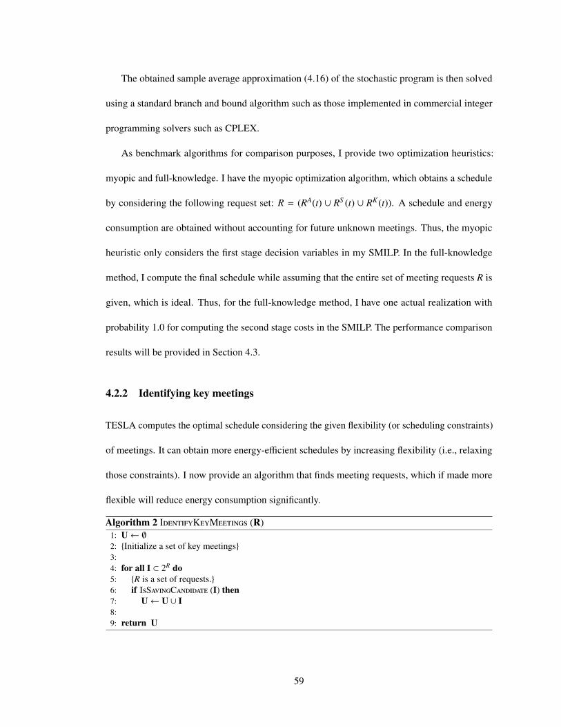
The obtained sample average approximation (4.16) of the stochastic program is then solved

using a standard branch and bound algorithm such as those implemented in commercial integer

programming solvers such as CPLEX.

As benchmark algorithms for comparison purposes, I provide two optimization heuristics:

myopic and full-knowledge. I have the myopic optimization algorithm, which obtains a schedule

by considering the following request set: R = (RA(t) ∪ RS (t) ∪ RK(t)). A schedule and energy

consumption are obtained without accounting for future unknown meetings. Thus, the myopic

heuristic only considers the first stage decision variables in my SMILP. In the full-knowledge

method, I compute the final schedule while assuming that the entire set of meeting requests R is

given, which is ideal. Thus, for the full-knowledge method, I have one actual realization with

probability 1.0 for computing the second stage costs in the SMILP. The performance comparison

results will be provided in Section 4.3.

4.2.2 Identifying key meetings

TESLA computes the optimal schedule considering the given flexibility (or scheduling constraints)

of meetings. It can obtain more energy-efficient schedules by increasing flexibility (i.e., relaxing

those constraints). I now provide an algorithm that finds meeting requests, which if made more

flexible will reduce energy consumption significantly.

Algorithm 2 IdentifyKeyMeetings (R)1: U← ∅2: {Initialize a set of key meetings}3:4: for all I ⊂ 2R do5: {R is a set of requests.}6: if IsSavingCandidate (I) then7: U← U ∪ I8:9: return U

59

Algorithm 3 IsSavingCandidate (I)1: VI ← CalExpEnergySavings(αI , {α′I,1, . . . , α

′I,k})

2: {αI is an initially given flexibility of meetings in I, and α′I,k is one of the desired flexibility options formeetings in I. CalExpEnergySavings computes energy gains, VI , by relaxing flexibility of meetingrequests in I.}

3:4: if |I| = 1 then5: if VI > τ then6: {If the computed energy gains VI is higher than a given threshold value τ, it is considered as a key

meeting.}7: return TRUE8: else9: return FALSE

10: else if |I| > 1 then11: {Recursively call IsSavingCandidate with possible subsets}12: for all i ∈ I do13: I’← I\{i}14: VI′ ← CalExpEnergySavings(αI′ , {α′I′,1, . . . , α

′I′,k})

15: if VI − VI′ > 0 then16: {Only if the energy savings are monotonically increasing by adding a meeting request i (or

monotonically decreasing by excluding a meeting request i), proceed}17: return IsSavingCandidate (I′)

Algorithm 2 describes the overall flow of the algorithm. I first initialize a set that will contain

key meetings identified by the algorithm (line 1). For each subset of the power set of meeting

requests R, I then examine whether or not the current meeting set I is a key meeting set by relying

on Algorithm 3 (line 6).

Algorithm 3 recursively determines if the given meeting set I is a candidate set that gives

significant potential energy savings. The meeting set I is detected as a key meeting set only if the

expected energy savings of meeting requests in I are monotonically increasing and show higher

energy improvements than the given threshold value (τ; a certain level of additional energy savings

that we desire to achieve with the selected key meetings) by relaxing their flexibility. To handle

this, I first compute the expected energy savings of the meeting set I when its flexibility level is

changed from the initial level αI to the desired level α′I assuming the other meetings’ flexibility

levels are fixed (line 1). The expected energy saving value of meeting set I, VI = (EαI − Eα′I)/EαI

60

(0 ≤ VI ≤ 1), where EαI is the current total energy consumption with the given level of flexibility

αI , and Eα′Iis the reduced total energy consumption if the meeting set I’s flexibility is changed

to one of k possible options, α′I,k, while others keep their given flexibility levels. In this work, I

consider a heuristic for setting the threshold value to investigate whether or not the current meeting

set I is an energy saving candidate set: a fixed single threshold value τ (line 5; e.g., 0.4 as a

universal threshold).

4.3 Empirical Validation

I evaluate the performance of TESLA and experimentally show that it can conserve energy by

providing more energy-efficient schedules in commercial buildings. At the end of this section,

I provide actual survey results that I have conducted on schedule flexibilities of real users. The

experiments were run on Intel Core2 Duo 2.53GHz CPU with 8GB main memory. I solved the

MILP formulations using CPLEX version 12.1. All techniques were evaluated for 100 independent

trials and I report the average values. Energy consumption was computed using the simulator

described earlier in Section 2.4.

4.3.1 Simulation Results

In this section, I provide the simulation results (i) to verify if flexibility really helps TESLA

compute energy-efficient schedules; (ii) to extensively evaluate the overall performance of the

SAA method while varying the sample size and flexibility; and (iii) to measure energy saving

benefits by identifying key meetings and by considering the cancellation rate.

61

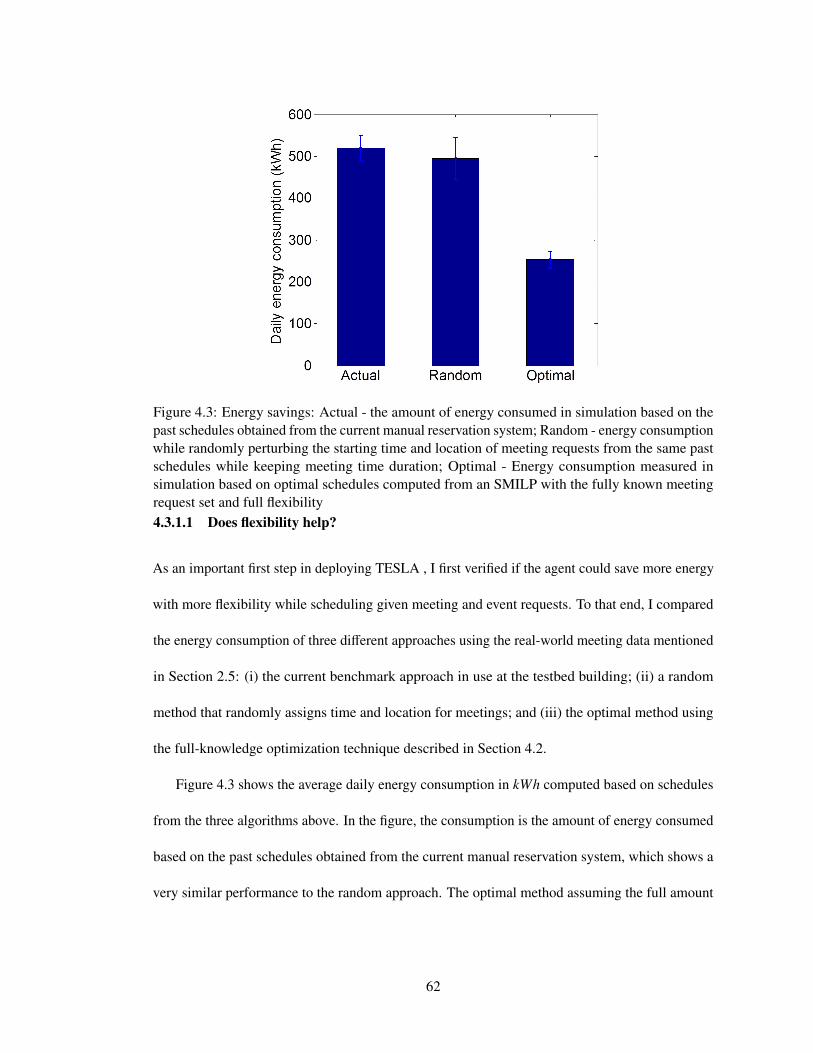
Figure 4.3: Energy savings: Actual - the amount of energy consumed in simulation based on thepast schedules obtained from the current manual reservation system; Random - energy consumptionwhile randomly perturbing the starting time and location of meeting requests from the same pastschedules while keeping meeting time duration; Optimal - Energy consumption measured insimulation based on optimal schedules computed from an SMILP with the fully known meetingrequest set and full flexibility4.3.1.1 Does flexibility help?

As an important first step in deploying TESLA , I first verified if the agent could save more energy

with more flexibility while scheduling given meeting and event requests. To that end, I compared

the energy consumption of three different approaches using the real-world meeting data mentioned

in Section 2.5: (i) the current benchmark approach in use at the testbed building; (ii) a random

method that randomly assigns time and location for meetings; and (iii) the optimal method using

the full-knowledge optimization technique described in Section 4.2.

Figure 4.3 shows the average daily energy consumption in kWh computed based on schedules

from the three algorithms above. In the figure, the consumption is the amount of energy consumed

based on the past schedules obtained from the current manual reservation system, which shows a

very similar performance to the random approach. The optimal method assuming the full amount

62

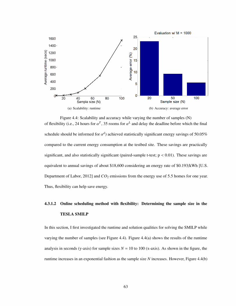
(a) Scalability: runtime (b) Accuracy: average error

Figure 4.4: Scalability and accuracy while varying the number of samples (N)of flexibility (i.e., 24 hours for αT , 35 rooms for αL and delay the deadline before which the final

schedule should be informed for αd) achieved statistically significant energy savings of 50.05%

compared to the current energy consumption at the testbed site. These savings are practically

significant, and also statistically significant (paired-sample t-test; p < 0.01). These savings are

equivalent to annual savings of about $18,600 considering an energy rate of $0.193/kWh [U.S.

Department of Labor, 2012] and CO2 emissions from the energy use of 5.5 homes for one year.

Thus, flexibility can help save energy.

4.3.1.2 Online scheduling method with flexibility: Determining the sample size in the

TESLA SMILP

In this section, I first investigated the runtime and solution qualities for solving the SMILP while

varying the number of samples (see Figure 4.4). Figure 4.4(a) shows the results of the runtime

analysis in seconds (y-axis) for sample sizes N = 10 to 100 (x-axis). As shown in the figure, the

runtime increases in an exponential fashion as the sample size N increases. However, Figure 4.4(b)

63

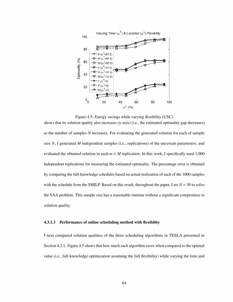
Figure 4.5: Energy savings while varying flexibility (USC)shows that its solution quality also increases (y-axis) (i.e., the estimated optimality gap decreases)

as the number of samples N increases. For evaluating the generated solution for each of sample

size N, I generated M independent samples (i.e., replications) of the uncertain parameters, and

evaluated the obtained solution in each m ∈ M replication. In this work, I specifically used 1,000

independent replications for measuring the estimated optimality. The percentage error is obtained

by comparing the full-knowledge schedules based on actual realization of each of the 1000 samples

with the schedule from the SMILP. Based on this result, throughout the paper, I set N = 50 to solve

the SAA problem. This sample size has a reasonable runtime without a significant compromise in

solution quality.

4.3.1.3 Performance of online scheduling method with flexibility

I next compared solution qualities of the three scheduling algorithms in TESLA presented in

Section 4.2.1. Figure 4.5 shows that how much each algorithm saves when compared to the optimal

value (i.e., full-knowledge optimization assuming the full flexibility) while varying the time and

64

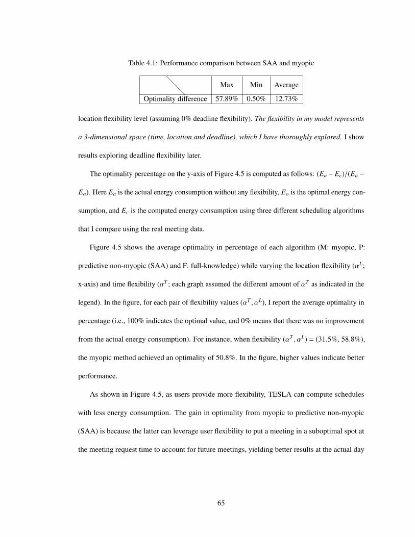
Table 4.1: Performance comparison between SAA and myopic

@@@

Max Min Average

Optimality difference 57.89% 0.50% 12.73%

location flexibility level (assuming 0% deadline flexibility). The flexibility in my model represents

a 3-dimensional space (time, location and deadline), which I have thoroughly explored. I show

results exploring deadline flexibility later.

The optimality percentage on the y-axis of Figure 4.5 is computed as follows: (Ea − Ec)/(Ea −

Eo). Here Ea is the actual energy consumption without any flexibility, Eo is the optimal energy con-

sumption, and Ec is the computed energy consumption using three different scheduling algorithms

that I compare using the real meeting data.

Figure 4.5 shows the average optimality in percentage of each algorithm (M: myopic, P:

predictive non-myopic (SAA) and F: full-knowledge) while varying the location flexibility (αL;

x-axis) and time flexibility (αT ; each graph assumed the different amount of αT as indicated in the

legend). In the figure, for each pair of flexibility values (αT , αL), I report the average optimality in

percentage (i.e., 100% indicates the optimal value, and 0% means that there was no improvement

from the actual energy consumption). For instance, when flexibility (αT , αL) = (31.5%, 58.8%),

the myopic method achieved an optimality of 50.8%. In the figure, higher values indicate better

performance.

As shown in Figure 4.5, as users provide more flexibility, TESLA can compute schedules

with less energy consumption. The gain in optimality from myopic to predictive non-myopic

(SAA) is because the latter can leverage user flexibility to put a meeting in a suboptimal spot at

the meeting request time to account for future meetings, yielding better results at the actual day

65

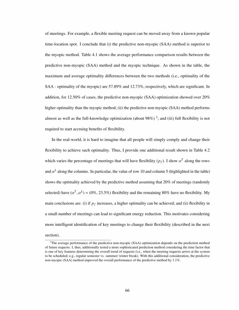
of meetings. For example, a flexible meeting request can be moved away from a known popular

time-location spot. I conclude that (i) the predictive non-myopic (SAA) method is superior to

the myopic method. Table 4.1 shows the average performance comparison results between the

predictive non-myopic (SAA) method and the myopic technique. As shown in the table, the

maximum and average optimality differences between the two methods (i.e., optimality of the

SAA - optimality of the myopic) are 57.89% and 12.73%, respectively, which are significant. In

addition, for 12.50% of cases, the predictive non-myopic (SAA) optimization showed over 20%

higher optimality than the myopic method; (ii) the predictive non-myopic (SAA) method performs

almost as well as the full-knowledge optimization (about 98%) 3; and (iii) full flexibility is not

required to start accruing benefits of flexibility.

In the real-world, it is hard to imagine that all people will simply comply and change their

flexibility to achieve such optimality. Thus, I provide one additional result shown in Table 4.2

which varies the percentage of meetings that will have flexibility (p f ). I show αT along the rows

and αL along the columns. In particular, the value of row 10 and column 5 (highlighted in the table)

shows the optimality achieved by the predictive method assuming that 20% of meetings (randomly

selected) have (αT , αL) = (0%, 23.5%) flexibility and the remaining 80% have no flexibility. My

main conclusions are: (i) if p f increases, a higher optimality can be achieved; and (ii) flexibility in

a small number of meetings can lead to significant energy reduction. This motivates considering

more intelligent identification of key meetings to change their flexibility (described in the next

section).3The average performance of the predictive non-myopic (SAA) optimization depends on the prediction method

of future requests. I, thus, additionally tested a more sophisticated prediction method considering the time factor thatis one of key features determining the overall trend of requests (i.e., when the meeting requests arrive at the systemto be scheduled; e.g., regular semester vs. summer/ winter break). With this additional consideration, the predictivenon-myopic (SAA) method improved the overall performance of the predictive method by 1.1%.

66

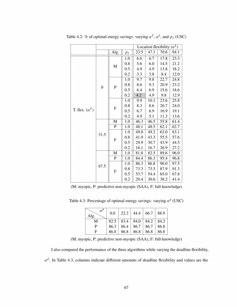
Table 4.2: % of optimal energy savings: varying αT , αL, and p f (USC)

T. flex. (αT )

Location flexibility (αL)Alg. p f 23.5 47.1 70.6 94.1

0

M

1.0 6.6 6.7 17.8 23.30.8 5.6 6.0 14.5 21.20.5 4.9 4.9 13.8 18.20.2 3.3 3.8 8.4 12.0

P

1.0 9.7 9.8 22.7 24.80.8 8.6 9.3 20.9 23.20.5 6.4 6.9 15.6 18.60.2 4.2 4.9 9.8 12.9

F

1.0 9.9 10.1 23.6 25.80.8 8.3 8.6 20.7 24.00.5 6.7 6.9 16.9 19.10.2 4.9 5.1 11.3 13.6

31.5

M 1.0 46.3 46.5 55.8 61.4P 1.0 48.1 48.5 62.1 62.7

F

1.0 49.0 49.2 63.0 63.10.8 41.9 43.3 55.5 57.60.5 29.9 30.7 43.9 44.50.2 16.1 16.7 26.9 27.2

67.5

M 1.0 81.8 82.5 89.6 96.0P 1.0 84.4 86.3 95.4 96.8

F

1.0 86.3 86.8 96.0 97.50.8 73.3 73.5 87.9 91.30.5 53.7 54.4 65.0 67.80.2 29.4 30.6 38.2 41.4

(M: myopic, P: predictive non-myopic (SAA), F: full-knowledge)

Table 4.3: Percentage of optimal energy savings: varying αd (USC)

HHHHHHAlg.αd

0.0 22.2 44.4 66.7 88.9

M 82.5 83.4 84.0 84.2 84.2P 86.3 86.4 86.7 86.7 86.8F 86.8 86.8 86.8 86.8 86.8

(M: myopic, P: predictive non-myopic (SAA), F: full-knowledge)

I also compared the performance of the three algorithms while varying the deadline flexibility,

αd. In Table 4.3, columns indicate different amounts of deadline flexibility and values are the

67

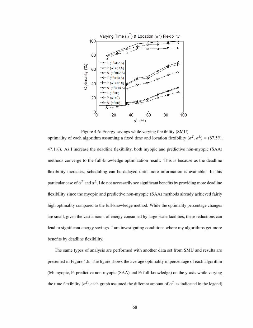
Figure 4.6: Energy savings while varying flexibility (SMU)optimality of each algorithm assuming a fixed time and location flexibility (αT , αL) = (67.5%,

47.1%). As I increase the deadline flexibility, both myopic and predictive non-myopic (SAA)

methods converge to the full-knowledge optimization result. This is because as the deadline

flexibility increases, scheduling can be delayed until more information is available. In this

particular case of αT and αL, I do not necessarily see significant benefits by providing more deadline

flexibility since the myopic and predictive non-myopic (SAA) methods already achieved fairly

high optimality compared to the full-knowledge method. While the optimality percentage changes

are small, given the vast amount of energy consumed by large-scale facilities, these reductions can

lead to significant energy savings. I am investigating conditions where my algorithms get more

benefits by deadline flexibility.

The same types of analysis are performed with another data set from SMU and results are

presented in Figure 4.6. The figure shows the average optimality in percentage of each algorithm

(M: myopic, P: predictive non-myopic (SAA) and F: full-knowledge) on the y-axis while varying

the time flexibility (αT ; each graph assumed the different amount of αT as indicated in the legend)

68

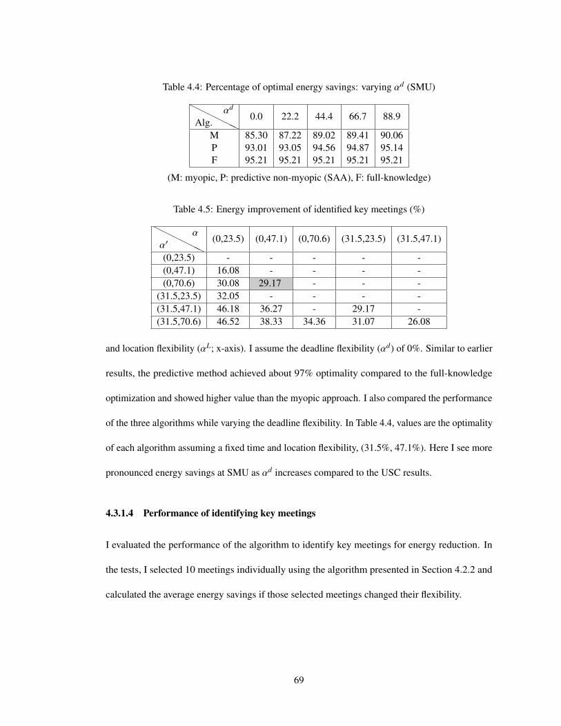
Table 4.4: Percentage of optimal energy savings: varying αd (SMU)

HHHHHHAlg.

αd0.0 22.2 44.4 66.7 88.9

M 85.30 87.22 89.02 89.41 90.06P 93.01 93.05 94.56 94.87 95.14F 95.21 95.21 95.21 95.21 95.21

(M: myopic, P: predictive non-myopic (SAA), F: full-knowledge)

Table 4.5: Energy improvement of identified key meetings (%)

HHHH

HHα′α

(0,23.5) (0,47.1) (0,70.6) (31.5,23.5) (31.5,47.1)

(0,23.5) - - - - -(0,47.1) 16.08 - - - -(0,70.6) 30.08 29.17 - - -

(31.5,23.5) 32.05 - - - -(31.5,47.1) 46.18 36.27 - 29.17 -(31.5,70.6) 46.52 38.33 34.36 31.07 26.08

and location flexibility (αL; x-axis). I assume the deadline flexibility (αd) of 0%. Similar to earlier

results, the predictive method achieved about 97% optimality compared to the full-knowledge

optimization and showed higher value than the myopic approach. I also compared the performance

of the three algorithms while varying the deadline flexibility. In Table 4.4, values are the optimality

of each algorithm assuming a fixed time and location flexibility, (31.5%, 47.1%). Here I see more

pronounced energy savings at SMU as αd increases compared to the USC results.

4.3.1.4 Performance of identifying key meetings

I evaluated the performance of the algorithm to identify key meetings for energy reduction. In

the tests, I selected 10 meetings individually using the algorithm presented in Section 4.2.2 and

calculated the average energy savings if those selected meetings changed their flexibility.

69

Table 4.5 shows the average energy savings as described for various flexibility transitions.

Columns indicate the initial level of flexibility (α = (αT , αL)) and rows show the requested level

of flexibility (α′ = (α′T , α′L)). For instance, the value in row 4 and column 3 (highlighted in the

table) indicates a 29.17% average energy savings improvement if flexibility of 10 key meetings

are changed from (0%, 47.1%) to (0%, 70.6%). An important interpretation of that results is

that changing the flexibility of key meetings, when those ones are from an appropriately chosen

set, contributed to significant energy savings. I also tested how much energy can be saved if key

meetings are chosen simultaneously rather than independently. Assuming the current flexibility

is (0%, 23.5%) (column 2 in Table 4.5), if I choose 10 key meetings at the same time using the

same algorithm presented in Section 4.2.2, the average energy savings were improved by 10.3%

(i.e., 44.48% of energy saving improvements on average). In the future, I will investigate another

heuristic to set a feasible threshold value based on a learned profile of user likelihood of changing

meeting flexibility.

4.3.1.5 Considering the cancellation rate

According to the real meeting data collected for eight months (January through August in 2012)

at USC, about 10.12% (3,245 out of 32,065) of the total meeting requests were canceled, which

gives me another insight to achieve further energy savings by utilizing this feature. To incorporate

this feature into my SMILP formulation 4, I change constraint (7) as follows:

Pr(∑

i′∈R\RU\{i}∑t+δi−1

t′=t xi′,l,t′ ≤ M(1 − xi,l,t)) ≥ 1 − αc

The constraint above is given in the form of the chance constrained programming that relaxes

the allocation restrictions (i.e., with a probability of αc, the given allocation restrictions can be

4Note that canceled meetings were not considered while scheduling meetings in the earlier results.

70

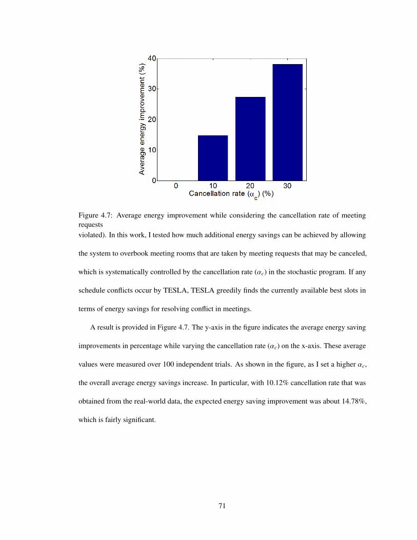
Figure 4.7: Average energy improvement while considering the cancellation rate of meetingrequestsviolated). In this work, I tested how much additional energy savings can be achieved by allowing

the system to overbook meeting rooms that are taken by meeting requests that may be canceled,

which is systematically controlled by the cancellation rate (αc) in the stochastic program. If any

schedule conflicts occur by TESLA, TESLA greedily finds the currently available best slots in

terms of energy savings for resolving conflict in meetings.

A result is provided in Figure 4.7. The y-axis in the figure indicates the average energy saving

improvements in percentage while varying the cancellation rate (αc) on the x-axis. These average

values were measured over 100 independent trials. As shown in the figure, as I set a higher αc,

the overall average energy savings increase. In particular, with 10.12% cancellation rate that was

obtained from the real-world data, the expected energy saving improvement was about 14.78%,

which is fairly significant.

71

Figure 4.8: Energy savings by TESLA: the percentage of energy savings per each energy consumerand factor4.4 Analysis: Savings due to TESLA

There are three major components that affect energy consumption in commercial buildings: HVACs

(accounting for 35% of the entire energy consumption in commercial buildings), lighting (27%),

and electronic devices (about 10%) [U.S. Department of Energy, 2010]. TESLA focuses on

these three energy consumers to save energy by computing energy-efficient schedules that exploit

key factors that affect energy consumption of each building component. Figure 4.8 shows the

percentage of energy savings per each energy consumer and factor in TESLA assuming an actually

measured time and location flexibility (αT , αL) = (25.34%, 16.05%) from surveys of real users.

For instance, as shown in the figure, 47.4% of energy savings by TESLA is achieved through

more energy-efficient operations of HVACs. More specifically, TESLA shifts meetings to suitable

smaller offices or non-peak time and packs meetings together, and those strategies result in a

significant energy reduction for HVACs.

4.4.1 HVACs

Key assumptions The following assumptions are made in TESLA :

72

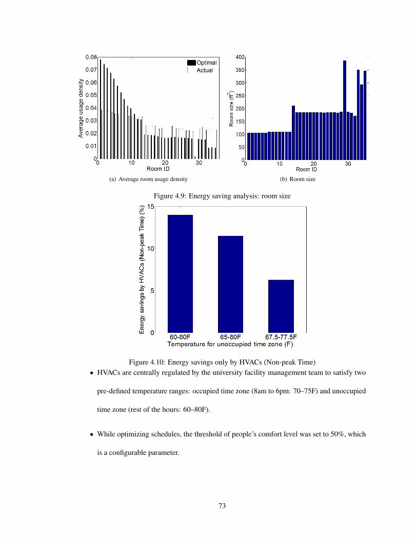
(a) Average room usage density (b) Room size

Figure 4.9: Energy saving analysis: room size

Figure 4.10: Energy savings only by HVACs (Non-peak Time)• HVACs are centrally regulated by the university facility management team to satisfy two

pre-defined temperature ranges: occupied time zone (8am to 6pm: 70–75F) and unoccupied

time zone (rest of the hours: 60–80F).

• While optimizing schedules, the threshold of people’s comfort level was set to 50%, which

is a configurable parameter.

73

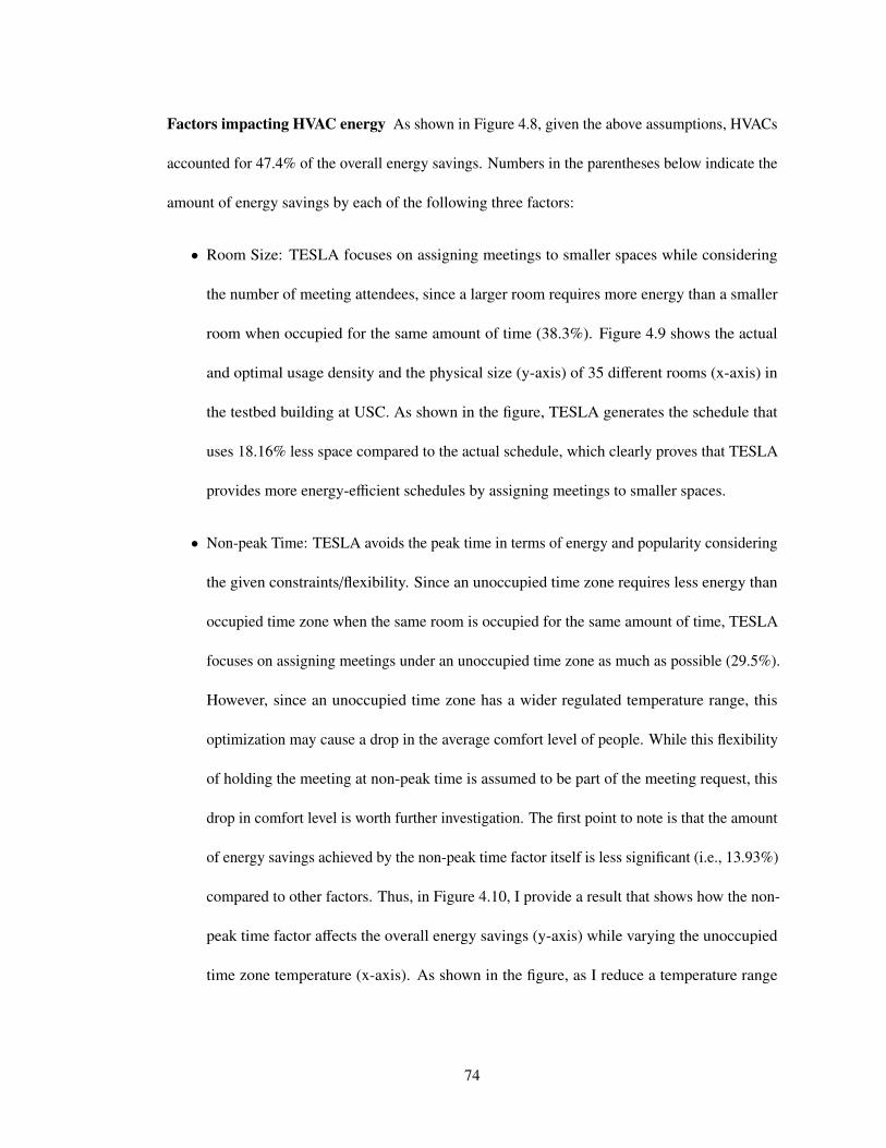
Factors impacting HVAC energy As shown in Figure 4.8, given the above assumptions, HVACs

accounted for 47.4% of the overall energy savings. Numbers in the parentheses below indicate the

amount of energy savings by each of the following three factors:

• Room Size: TESLA focuses on assigning meetings to smaller spaces while considering

the number of meeting attendees, since a larger room requires more energy than a smaller

room when occupied for the same amount of time (38.3%). Figure 4.9 shows the actual

and optimal usage density and the physical size (y-axis) of 35 different rooms (x-axis) in

the testbed building at USC. As shown in the figure, TESLA generates the schedule that

uses 18.16% less space compared to the actual schedule, which clearly proves that TESLA

provides more energy-efficient schedules by assigning meetings to smaller spaces.

• Non-peak Time: TESLA avoids the peak time in terms of energy and popularity considering

the given constraints/flexibility. Since an unoccupied time zone requires less energy than

occupied time zone when the same room is occupied for the same amount of time, TESLA

focuses on assigning meetings under an unoccupied time zone as much as possible (29.5%).

However, since an unoccupied time zone has a wider regulated temperature range, this

optimization may cause a drop in the average comfort level of people. While this flexibility

of holding the meeting at non-peak time is assumed to be part of the meeting request, this

drop in comfort level is worth further investigation. The first point to note is that the amount

of energy savings achieved by the non-peak time factor itself is less significant (i.e., 13.93%)

compared to other factors. Thus, in Figure 4.10, I provide a result that shows how the non-

peak time factor affects the overall energy savings (y-axis) while varying the unoccupied

time zone temperature (x-axis). As shown in the figure, as I reduce a temperature range

74

for the unoccupied time zone, the amount of energy savings by the non-peak time factor

decreases, but TESLA can still achieve meaningful energy savings while satisfying the given

comfort level constraint. Furthermore, TESLA provides a flexible architecture that allows

people to configure the temperature value accordingly under different situations.

• Packing Meetings: TESLA focused on packing meetings together in terms of the time

interval between meetings in the same room. When a meeting ends, the room is conditioned

to a pre-defined environment. This built-up thermal momentum can benefit later meetings

scheduled in the same room in close proximity by reducing the number of changes of HVAC

operations, which saves much more energy (32.2%).

4.4.2 Lighting

Key assumptions The following assumptions are made in TESLA :

• The standard nominal values were used for the lighting configuration in spaces.

• When the room was occupied, the full (100%) lighting level was considered.

• When the room was unoccupied, 0% lighting level was considered.

Factors impacting lighting energy As shown in Figure 4.8, given the above assumptions, the

lighting sources accounted for 37.5% of the overall energy savings. The entire energy savings

are caused by different room size; specifically, TESLA focuses on assigning meetings to smaller

spaces while considering the number of meeting attendees, since a larger room requires more

energy than a smaller room when occupied for the same amount of time (see Figure 4.9).

75

4.4.3 Electronics

Key assumptions The following assumptions are made in TESLA :

• Assumed average number of devices in each room was considered to calculate the correct

energy consumption. 5

• When the room was occupied, 80% of the devices were used.

• When the room was unoccupied, 0% of the devices were used.

Factors impacting electronics energy As shown in Figure 4.8, given the above assumptions,

the electronics accounted for 15.1% of the overall energy savings. The entire energy savings

are caused by different room size; specifically, TESLA focuses on assigning meetings to smaller

spaces while considering the number of meeting attendees, since a larger room has more devices

in the testbed building, and thus it requires more energy than a smaller room when occupied for

the same amount of time (see Figure 4.9).

4.5 Human Subject Experiments

The goal of human subject experiments is to support the results provided in the previous section

by answering several questions: (i) are people flexible in real situations?; (ii) how flexible are

people in modifying their requests?; (iii) will people in the identified key meetings actually agree

to change their flexibility to contribute energy savings?; and (iv) what would be an effective way

for an agent to persuade people? To answer these, I measure the amount of reported flexibility

change while varying feedback about the energy usage.

5While evaluating TESLA, I considered the assumed average number of electronic devices including the actualnumber of devices existing in each room as well as the average number of devices that people bring with them.

76

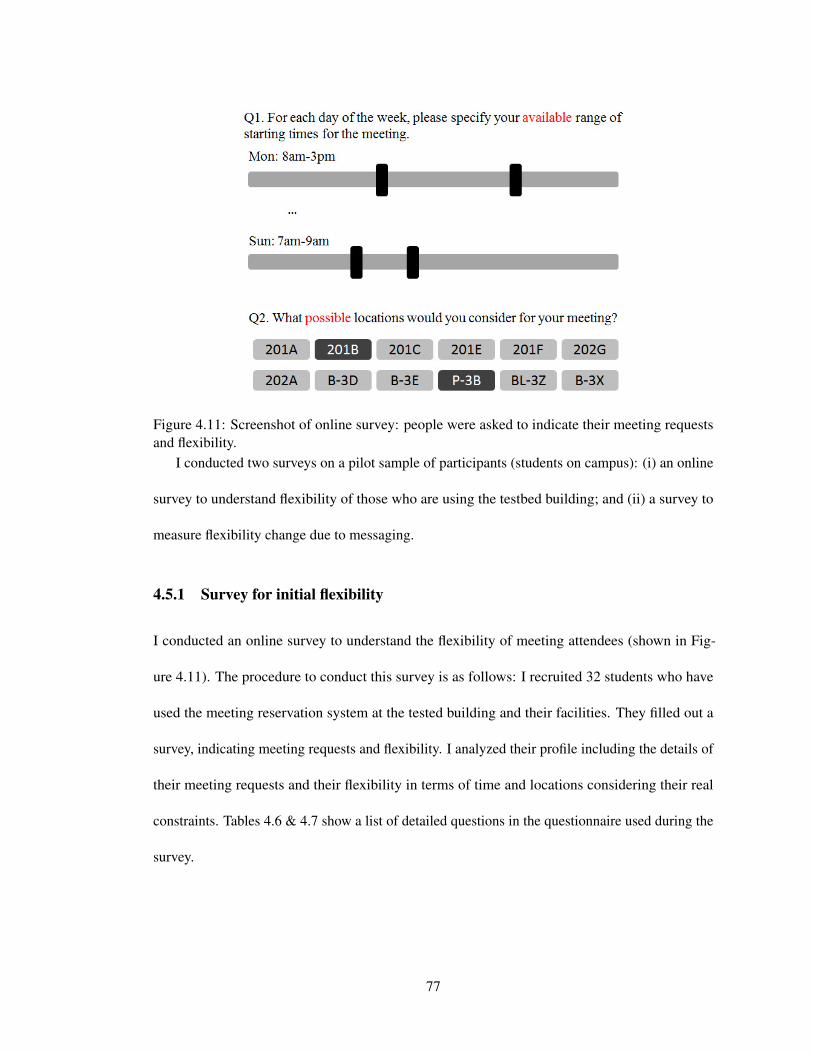
Figure 4.11: Screenshot of online survey: people were asked to indicate their meeting requestsand flexibility.

I conducted two surveys on a pilot sample of participants (students on campus): (i) an online

survey to understand flexibility of those who are using the testbed building; and (ii) a survey to

measure flexibility change due to messaging.

4.5.1 Survey for initial flexibility

I conducted an online survey to understand the flexibility of meeting attendees (shown in Fig-

ure 4.11). The procedure to conduct this survey is as follows: I recruited 32 students who have

used the meeting reservation system at the tested building and their facilities. They filled out a

survey, indicating meeting requests and flexibility. I analyzed their profile including the details of

their meeting requests and their flexibility in terms of time and locations considering their real

constraints. Tables 4.6 & 4.7 show a list of detailed questions in the questionnaire used during the

survey.

77

Table 4.6: Basic Profile Questionnaire

Question Answer (Scale)Q1. Gender? Male / FemaleQ2. Position at USC? Undergraduate / Graduate / Staff / Faculty

Q3. Age?20 or under / 21–25 / 26–30 / 31–35 /

36–40 / 41 or aboveQ4. How many times, on average, do you use

0 – 10 or moreUSC Leavey collaborative workrooms per week?Q5. How many meeting attendees, on average,

1 – 10 or moredo you have?Q6. What is your average meeting time duration?

1 – 5 or more(in hour)Q7. How much do you consider energy savings

1 (Do not consider at all) – 7 (Extremely consider)while requesting scheduling meetings?Q8. I consider myself an environmentalist. 1 (Disagree) – 7 (Agree)

Table 4.7: Survey I: Questionnaire

Assumption (A)Let us assume that you would like to schedule a meeting next week using the centralmeeting reservation system, which is currently used at USC Leavey library.

Question (Q)

Q1. What is your preferred time range to start the meeting on each day of the week?(Note: Consider your actual class and other meeting constraints while answering this.)Q2. What locations do you prefer for your meeting among the rooms that you chosen?For your information, the number in the parentheses indicates the maximumcapacity of each room.(Note: Please try to answer this based on your past experience at USC Leavey library.)

Figure 5.8 shows the distribution of the time and location flexibility. The x-axis shows the

discretized flexibility level and their corresponding frequency in percentage is provided on the

y-axis. People reported varied levels of time and location flexibility. The average time flexibility

(αT ) was 25.34% and the measured minimum and maximum time flexibility were 9.86% and

42.86%, respectively. The average location flexibility (αL) was 16.05% and its range was 0 to

38.24%. This survey result clearly shows that people have fairly diverse flexibility levels and

78

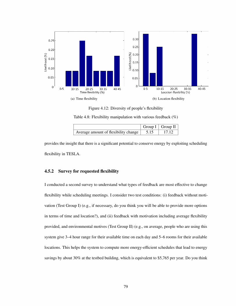
(a) Time flexibility (b) Location flexibility

Figure 4.12: Diversity of people’s flexibility

Table 4.8: Flexibility manipulation with various feedback (%)

Group I Group IIAverage amount of flexibility change 5.15 17.12

provides the insight that there is a significant potential to conserve energy by exploiting scheduling

flexibility in TESLA.

4.5.2 Survey for requested flexibility

I conducted a second survey to understand what types of feedback are most effective to change

flexibility while scheduling meetings. I consider two test conditions: (i) feedback without moti-

vation (Test Group I) (e.g., if necessary, do you think you will be able to provide more options

in terms of time and location?), and (ii) feedback with motivation including average flexibility

provided, and environmental motives (Test Group II) (e.g., on average, people who are using this

system give 3–4 hour range for their available time on each day and 5–6 rooms for their available

locations. This helps the system to compute more energy-efficient schedules that lead to energy

savings by about 30% at the testbed building, which is equivalent to $5,765 per year. Do you think

79

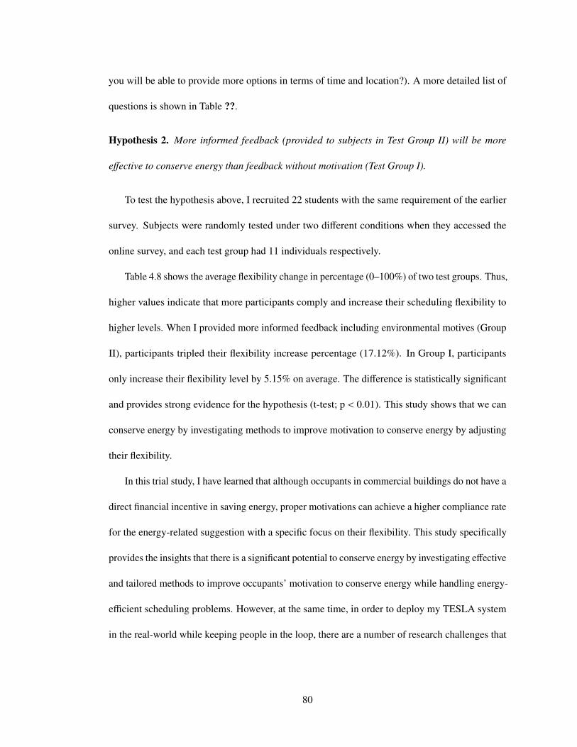
you will be able to provide more options in terms of time and location?). A more detailed list of

questions is shown in Table ??.

Hypothesis 2. More informed feedback (provided to subjects in Test Group II) will be more

effective to conserve energy than feedback without motivation (Test Group I).

To test the hypothesis above, I recruited 22 students with the same requirement of the earlier

survey. Subjects were randomly tested under two different conditions when they accessed the

online survey, and each test group had 11 individuals respectively.

Table 4.8 shows the average flexibility change in percentage (0–100%) of two test groups. Thus,

higher values indicate that more participants comply and increase their scheduling flexibility to

higher levels. When I provided more informed feedback including environmental motives (Group

II), participants tripled their flexibility increase percentage (17.12%). In Group I, participants

only increase their flexibility level by 5.15% on average. The difference is statistically significant

and provides strong evidence for the hypothesis (t-test; p < 0.01). This study shows that we can

conserve energy by investigating methods to improve motivation to conserve energy by adjusting

their flexibility.

In this trial study, I have learned that although occupants in commercial buildings do not have a

direct financial incentive in saving energy, proper motivations can achieve a higher compliance rate

for the energy-related suggestion with a specific focus on their flexibility. This study specifically

provides the insights that there is a significant potential to conserve energy by investigating effective

and tailored methods to improve occupants’ motivation to conserve energy while handling energy-

efficient scheduling problems. However, at the same time, in order to deploy my TESLA system

in the real-world while keeping people in the loop, there are a number of research challenges that

80

have to be addressed. Most notably, in a commercial setup where people do not have a direct

financial incentive to save energy, a different incentive mechanism to effectively motivate them

and keep them as active participants in energy saving activities might potentially be required;

determining the importance of such mechanisms or if they are needed in the first place is a topic

for future work [Abrahmase et al., 2005; Anderson et al., 2012; Carrico and Riemer, 2011; Faruqui

et al., 2010; Wood and Neal, 2009]. Over time, people will be able to observe the impact of their

input (e.g., flexibility) while scheduling meetings and whether or not people engaged with TESLA

on a day-to-day basis will provide flexibility to the extent they could remains to be determined.

Thus, while this paper has provided a critical first step in flexibility-based energy savings, and

provided algorithms to accomplish such savings, a future implementation will need to take the

next step to investigate topics such as motivation and incentives.

81

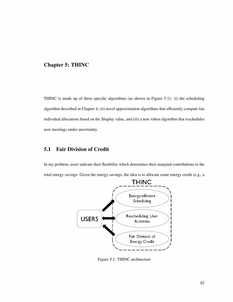
Chapter 5: THINC

THINC is made up of three specific algorithms (as shown in Figure 5.1): (i) the scheduling

algorithm described in Chapter 4, (ii) novel approximation algorithms that efficiently compute fair

individual allocations based on the Shapley value, and (iii) a new robust algorithm that reschedules

user meetings under uncertainty.

5.1 Fair Division of Credit

In my problem, users indicate their flexibility which determines their marginal contributions to the

total energy savings. Given the energy savings, the idea is to allocate some energy credit (e.g., a

Figure 5.1: THINC architecture

82

significant portion of the savings) to individual users. In allocating credit, equal allocation may not

be perceived as fair as shown in [Abrahmase et al., 2005; Hassett and Metcalf, 1995] and my survey

results (Section 5.3.1). Furthermore, proportional allocation based on flexibility fails in practice

because the amount of flexibility does not necessarily reflect users’ true contributions to energy

savings. For example, out of two users A and B, let A offer 80% flexibility late at night, while

B offers 40% flexibility during peak hours. Since B requests a meeting at a peak time/location

(where given individual flexibility can be jointly exploited with others for more energy savings,

e.g., back-to-back effect described in Section 4.2) and A at an off-peak time/location, flexibility of

B may lead to more energy savings as compared to A due to the exploitation of joint flexibility.

Therefore, flexibility of B has a greater effect in this case and hence B’s compensation should be

higher. If we used proportional allocation, A would get higher compensation which will not be

perceived as fair.

My energy-cost minimizing scheduling problem can be framed as a coalitional game, (N, v),

where:

• N is a finite set of players, indexed by i. In my case, N indicates the set of meeting requests.

• S is a coalition ⊆ N. In my case, it is a subset of meeting requests that provide flexibility.1

So a coalition is formed from meetings that provide flexibility.

• v : 2N 7→ R is a characteristic function. In my case, v(S ) is the total energy-savings

obtained when requests in S are flexible and requests in N \ S are not flexible. Formally:

v(S ) = e(S ) − e(S ), where e(S ) is the energy consumption when meeting requests in S

provide flexibility and e(S ) is the energy consumption when requests in S do not provide

1This definition can be easily extended to the case where each separate coalition is defined based on a discretizedlevel of flexibility.

83

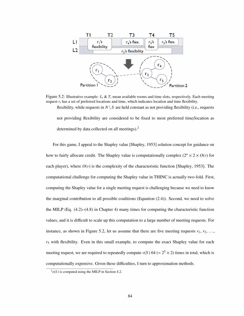
Figure 5.2: Illustrative example: Li & Ti mean available rooms and time slots, respectively. Each meetingrequest ri has a set of preferred locations and time, which indicates location and time flexibility.

flexibility, while requests in N \ S are held constant as not providing flexibility (i.e., requests

not providing flexibility are considered to be fixed to most preferred time/location as

determined by data collected on all meetings).2

For this game, I appeal to the Shapley value [Shapley, 1953] solution concept for guidance on

how to fairly allocate credit. The Shapley value is computationally complex (2n × 2 × O(v) for

each player), where O(v) is the complexity of the characteristic function [Shapley, 1953]. The

computational challenge for computing the Shapley value in THINC is actually two-fold. First,

computing the Shapley value for a single meeting request is challenging because we need to know

the marginal contribution to all possible coalitions (Equation (2.4)). Second, we need to solve

the MILP (Eq. (4.2)–(4.8) in Chapter 4) many times for computing the characteristic function

values, and it is difficult to scale up this computation to a large number of meeting requests. For

instance, as shown in Figure 5.2, let us assume that there are five meeting requests r1, r2, . . .,

r5 with flexibility. Even in this small example, to compute the exact Shapley value for each

meeting request, we are required to repeatedly compute v(S ) 64 (= 25 × 2) times in total, which is

computationally expensive. Given these difficulties, I turn to approximation methods.

2e(S ) is computed using the MILP in Section 4.2.

84

5.1.1 Approximate Shapley computation

I efficiently approximate the Shapley value using: (i) sampling and (ii) graph partitioning.

Sampling: Random sampling can be used to approximate the Shapley value [Castro et al., 2009;

Fatima et al., 2008; Mann and Llyod, 1960; Owen, 1972]. In particular, Castro et al. [Castro

et al., 2009] presented the ApproShapley algorithm, a sampling mechanism for polynomial-

time approximation of the Shapley value. In ApproShapley, the characteristic function value is

repeatedly computed (m × 2) times per each player, where m is the number of samples. In the

above example, for each meeting request, we now only need to compute v(S ) 20 (= 10 × 2) times

with 10 samples, which is smaller than the exact Shapley value computation.

Graph Partitioning: In addition to using ApproShapley, we can partition the entire meeting

request set into multiple independent subsets, which reduces the overall computational burden.

This idea is justified by the inessential axiom defined below. The entire meeting request set R can

be represented as an unweighted undirected graph denoted G = (V, E). As shown in Figure 5.2,

each vertex in V represents a meeting request in R. If the flexibility ranges of any two meeting

requests overlap, then those meeting requests are connected as an unordered pair in the graph

defining the edge set E (with edge weight defined by the amount of overlap). For example,

in Figure 5.2, r2 and r3 overlap, defining an edge between them. We can define a notion of

independence between two meeting request subsets Rm and Rn, where Rm,Rn ⊆ R, as follows. Two

important technical lemmas then follow:

Definition 2. Independence: Rm and Rn are independent if e(Rm ∪ Rn) = e(Rm) + e(Rn), where

e(R) is the energy consumption of the given meeting request set R.3

3Please note that we need to run the MILP to test for independence.

85

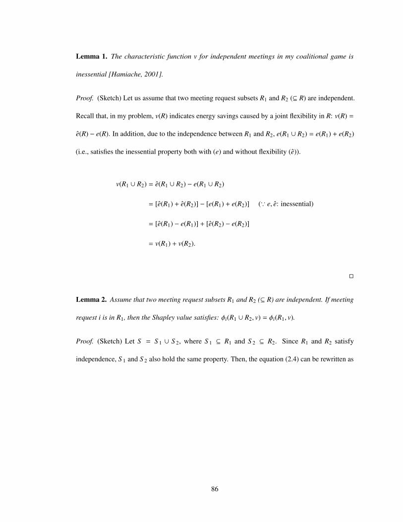
Lemma 1. The characteristic function v for independent meetings in my coalitional game is

inessential [Hamiache, 2001].

Proof. (Sketch) Let us assume that two meeting request subsets R1 and R2 (⊆ R) are independent.

Recall that, in my problem, v(R) indicates energy savings caused by a joint flexibility in R: v(R) =

e(R) − e(R). In addition, due to the independence between R1 and R2, e(R1 ∪ R2) = e(R1) + e(R2)

(i.e., satisfies the inessential property both with (e) and without flexibility (e)).

v(R1 ∪ R2) = e(R1 ∪ R2) − e(R1 ∪ R2)

= [e(R1) + e(R2)] − [e(R1) + e(R2)] (∵ e, e: inessential)

= [e(R1) − e(R1)] + [e(R2) − e(R2)]

= v(R1) + v(R2).

�

Lemma 2. Assume that two meeting request subsets R1 and R2 (⊆ R) are independent. If meeting

request i is in R1, then the Shapley value satisfies: φi(R1 ∪ R2, v) = φi(R1, v).

Proof. (Sketch) Let S = S 1 ∪ S 2, where S 1 ⊆ R1 and S 2 ⊆ R2. Since R1 and R2 satisfy

independence, S 1 and S 2 also hold the same property. Then, the equation (2.4) can be rewritten as

86

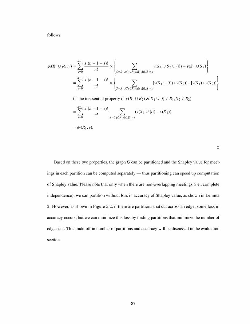
follows:

φi(R1 ∪ R2, v) =

n−1∑s=0

s!(n − 1 − s)!n!

×

∑S =S 1∪S 2⊆R1∪R2\{i},|S |=s

v(S 1 ∪ S 2 ∪ {i}) − v(S 1 ∪ S 2)

=

n−1∑s=0

s!(n − 1 − s)!n!

×

∑S =S 1∪S 2⊆R1∪R2\{i},|S |=s

[v(S 1 ∪ {i})+v(S 2)]−[v(S 1)+v(S 2)]

(∵ the inessential property of v(R1 ∪ R2) & S 1 ∪ {i} ∈ R1, S 2 ∈ R2)

=

n−1∑s=0

s!(n − 1 − s)!n!

∑S =S 1⊆R1\{i},|S |=s

(v(S 1 ∪ {i}) − v(S 1))

= φi(R1, v).

�

Based on these two properties, the graph G can be partitioned and the Shapley value for meet-

ings in each partition can be computed separately — thus partitioning can speed up computation

of Shapley value. Please note that only when there are non-overlapping meetings (i.e., complete

independence), we can partition without loss in accuracy of Shapley value, as shown in Lemma

2. However, as shown in Figure 5.2, if there are partitions that cut across an edge, some loss in

accuracy occurs; but we can minimize this loss by finding partitions that minimize the number of

edges cut. This trade-off in number of partitions and accuracy will be discussed in the evaluation

section.

87

5.1.2 Approximate characteristic value computation

In my work, the characteristic function, v(S ), itself is computationally intensive because it is an

MILP. To compute the Shapley value, we need to solve multiple instances of these MILPs. Thus, I

introduce efficient methods to approximate the characteristic value computation by relying on (i)

caching and (ii) LP relaxation.

Caching: This technique exploits the following property:

Definition 3. Exchangeability: v is exchangeable if, for every permutation π of S ⊆ N, v(S ) =

v(π(S )) [Aldous, 1985].

v(S ) in my problem is exchangeable. Thus, we can further speed up the Shapley value

computation by storing evaluations of v(S ). In this way, the characteristic function value of each

coalition and all its permutations is computed only once.

LP Relaxation: It is natural then to use MILP relaxation to approximately compute v(S ). I

specifically relax the integrality constraint (4.8) in (MILP) to 0 ≤ xi,l,t ≤ 1 for getting a linear

program (LP). The optimal solution of (LP) is a lower bound on the optimal value of (MILP). I

empirically show the strength of the LP relaxation for my specific MILP in the evaluation section.

5.2 THINC Rescheduling Algorithm

While THINC performs energy-efficient scheduling, it may perceive that shifting some carefully

selected meetings can lead to significant energy savings. THINC then makes suggestions to

involved users on how to best reschedule their meetings while ensuring a balance between energy

savings and user comfort (hence, multi-objective MDP). We cannot know the exact likelihood

that users will comply with suggestions, and we may also be uncertain about the reward from

88

energy-savings and user comfort (hence the model uncertainty). I provide new algorithms for

BM-MDPs in THINC in addressing these challenges.

As a concrete example of how THINC can reschedule meetings, suppose two meeting requests

(r1 and r2), which are originally scheduled in (10am, Room A) and (10am, Room B) respectively,

are identified for rescheduling. THINC’s policy may suggest r1 and r2 to be rescheduled to

different times but the same location as r3 (12pm, Room B). This way, the agent can consolidate

all three meetings (r1 – r3) together in a smaller room B which is less expensive to heat/cool.

Now, assuming that r1 can only be scheduled either at 10am or 12pm, the best scenario is to

reschedule r1 to (10am, Room B) and r2 to (11am, Room B) so that all three meetings only use

Room B from 10am to 12pm, sequentially. Let us also assume that the r2 is less likely to agree to

reschedule, and the likelihood of r1 and r3 is high. In this situation, if r2 does not comply (given

low likelihood) then THINC’s computed policy needs to provide an alternative action given r2’s

refusal, while considering the likelihood of acceptance for this alternative. In particular, THINC

instead suggests rescheduling r3 to (11am, Room B) and r1 to (12pm, Room B), which is highly

likely to be accepted by users. In addition, if an unexpected new meeting request (r4) arrives and

is identified as an energy-consuming meeting to be rescheduled, then the rescheduling policy may

need to change.

I thus provide two novel algorithms in this work: (i) a robust multi-objective MDP algorithm

for solving BM-MDPs which allows for stochasticity in user response at planning time and (ii)

replanning methods to handle execution-time uncertainty (e.g., due to the arrival of r4). I first

discuss my robust multi-objective MDP algorithm. Earlier work [Kwak et al., 2012a] provides

“optimistic” or “pessimistic” heuristics to solve BM-MDPs, but without any performance guarantee.

Instead, my present robust BM-MDP can be solved exactly by finite horizon value iteration. First,

89

the robust optimal expected value is computed using the robust value iteration [Bagnell et al.,

2001] for each objective. Next, given an optimal robust value for each objective, the regret across

all objectives is computed. Lastly, a robust policy that minimizes the regret is chosen.

STEP I: Computing the robust optimal value for each objective: I denote the (finite) state

space (set of meeting requests) by S and the (finite) space of actions by A (i.e., the set of energy-

efficient meeting rescheduling suggestions by THINC). I fix a finite time horizon T = {0, 1, . . . ,T },

i.e., my work always uses a T period lookahead policy when (re)planning. Let I index a set

of reward functions ri : S × A → R to allow for multiple objectives. These include energy

efficiency and comfort of different users. We let τ ( j|s, a) denote the transition probabilities, the

probability of transitioning to state j ∈ S given (s, a). For each state and action, we let Ri (s, a)

denote the uncertainty set for reward ri, and we let τ (s, a) denote the uncertainty set for τ. The

uncertainty set defines possible realizations of the uncertain parameters, e.g., uncertainty set of

reward for comfort may be the interval say 1–5. For emphasis, both of these uncertainty sets

depend on the current state-action pair. We let τ = {τ (s, a)}s, a and Ri ={Ri (s, a)

}s, a

be the

collections of these uncertainty sets. For fixed i ∈ I, I want to maximize the worst-case reward,

i.e., maxa∈A minτ∈τ, ri∈Ri Eπτ[∑T

t=0 γtri (st)

], where Eπτ [·] explicitly indicates the dependence on the

transition probabilities and the policy, and st is the state at time t. Because the uncertainty sets

only depend on the current state-action pair, the Bellman equation for the above robust MDP can

be written as follows:

V it (s) = max

a∈Amin

τ∈τ(s,a), ri∈Ri(s,a)

ri (s)+γ∑j∈S

τ ( j|s, a) V it+1 ( j)

90

where V it is the time t value function. The values

{V i

t (s)}

s∈S , t∈Tcan be computed through maximin

value iteration since we have a finite time horizon [Bagnell et al., 2001].

STEP II: Computing the regret across all objectives: Because my problem is multi-objective,

I want a policy that accounts for all objectives i ∈ I. So, I introduce a notion of regret that

accounts for all objectives. I will use a vector-valued value function {Wt}t∈T ⊂ R|I| where Wt (s) =(

W it (s)

)i∈I,∀t ∈ T. For a given policy π (which is different from the policy that computed V i

t in

Step I), the quantity

maxi∈I

minτ∈τ(s,a), ri∈Ri(s,a)

ri (s)+γ∑j∈S

τ ( j|s, a) W it+1 ( j)−V i

t (s)

is the regret at time t in state s ∈ S for action a, where V i

t for each objective i is given as a constant

from Step I. Notice that this definition takes the minimum over all reward functions. The quantity

ri (s) + γ∑

j∈S τ ( j|s, a) W it+1 ( j) is the value for objective i, and V i

t (s) is the optimal value for

objective i.

STEP III: Choosing the robust policy that minimizes the regret: In state s at time t I choose

a regret minimizing action

π∗t (s) ∈ arg mina∈A

maxi∈I

minτ∈τ(s,a), ri∈Ri(s,a)

ri (s) + γ∑j∈S

τ ( j|s, a) W it+1 ( j) − V i

t (s)

and then I set

W it (s) = min

τ∈τ(s,π∗t (s)), r∈Ri(s,π∗t (s))

ri (s) + γ∑j∈S

τ(j|s, π∗t (s)

)W i

t+1 ( j)

, (∀s ∈ S , ∀i ∈ I).

91

The optimal action is chosen in consideration of all objectives i ∈ I, and then each component of

Wt is updated separately assuming the same optimal action is taken in each update. The resulting

policy π∗ =(π∗t

)t∈T is the optimal regret minimizing policy.

During the execution of such a policy, THINC sometimes encounters unexpected situations,

e.g., in the example above r4 arrived when it was not part of the initial BM-MDP state-space and

was an energy-consuming meeting in need of rescheduling. THINC’s key insight is to continue

to use the current BM-MDP policy to the extent possible, replanning only when new meetings

are seen to potentially interfere with that policy. One alternative approach is to avoid BM-MDP

planning altogether and only react to the current state. Another alternative is to stay completely

committed to the original policy until completion while ignoring the new meetings. THINC rejects

both of these extreme approaches and occupies a middle ground: it does use a BM-MDP policy,

but when new meetings arrive, it checks if they interfere with the current policy. Specifically, the

majority of incoming meeting requests propose locations and times that do not affect the current

policy, allowing THINC to accrue the benefits of its optimal planning (carried out to completion)

in majority of cases; but THINC will occasionally compute a new policy if the new meetings are

seen to potentially interfere. Using real meeting arrival data in a large university building, THINC

demonstrates that this “middle-ground” approach outperforms the two extreme approaches in my

domain (Section 5.3.2).

5.3 Empirical Validation

I evaluate THINC in this section. For the evaluation, I built upon the simulation testbed developed

in [Kwak et al., 2012a] by using a large data set of real meeting requests and building statistics

92

collected from the testbed building. For experiments with meetings, I selected data from the library,

where 100 meetings may arrive per day. The experiments were run on Intel Core2 Duo 2.53GHz

CPU with 8GB memory. I solved MILPs using CPLEX version 12.1. I ran all algorithms for 100

independent trials and report average values.

5.3.1 Shapley Value Evaluation

5.3.1.1 Fair Division: Why Shapley Value?

The Shapley value gives a theoretically fair allocation and has been previously applied in energy

domains [Alam et al., 2013; Stein et al., 2012]. However, I wished to check user reactions in my

own domain, i.e., whether people believe that the Shapley value produces fair allocations of energy

credits. So, I launched a survey on Amazon Mechanical Turk (AMT) and collected data for 53

unique samples. I showed survey participants two different allocations: one based on Shapley

value and the other based on equal division. I then asked survey participants to rate fairness of

each allocation scheme on a scale of 1 to 7 while varying information, where 7 indicates high

fairness. I found that people perceive Shapley value based allocations to be more fair than those

based on equal division. The average fairness rating over all users for Shapley based allocation is

5.2, as compared to 3.6 for equal division and this result is statistically significant (paired t-test; p

≤ 0.04).

5.3.1.2 Approximation

We already know that the Shapley value is computationally expensive for the setting used in my

work. As shown in Figure 5.3 for the illustration purpose, as the number of meetings (x-axis)

increases from 5 to 100, the average runtime (y-axis) of the Shapley value computation increases

93

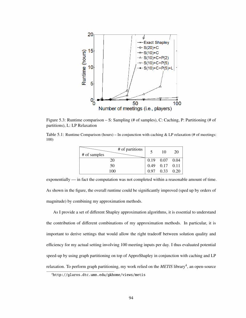
Figure 5.3: Runtime comparison – S: Sampling (# of samples), C: Caching, P: Partitioning (# ofpartitions), L: LP Relaxation

Table 5.1: Runtime Comparison (hours) – In conjunction with caching & LP relaxation (# of meetings:100)

hhhhhhhhhhhhhhhhh# of samples# of partitions

5 10 20

20 0.19 0.07 0.0450 0.49 0.17 0.11100 0.97 0.33 0.20

exponentially — in fact the computation was not completed within a reasonable amount of time.

As shown in the figure, the overall runtime could be significantly improved (sped up by orders of

magnitude) by combining my approximation methods.

As I provide a set of different Shapley approximation algorithms, it is essential to understand

the contribution of different combinations of my approximation methods. In particular, it is

important to derive settings that would allow the right tradeoff between solution quality and

efficiency for my actual setting involving 100 meeting inputs per day. I thus evaluated potential

speed-up by using graph partitioning on top of ApproShapley in conjunction with caching and LP

relaxation. To perform graph partitioning, my work relied on the METIS library4, an open-source

4http://glaros.dtc.umn.edu/gkhome/views/metis

94

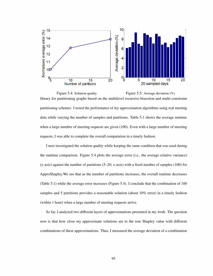
Figure 5.4: Solution quality Figure 5.5: Average deviation (%)

library for partitioning graphs based on the multilevel recursive-bisection and multi-constraint

partitioning schemes. I tested the performance of my approximation algorithms using real meeting

data while varying the number of samples and partitions. Table 5.1 shows the average runtime

when a large number of meeting requests are given (100). Even with a large number of meeting

requests, I was able to complete the overall computation in a timely fashion.

I next investigated the solution quality while keeping the same condition that was used during

the runtime comparison. Figure 5.4 plots the average error (i.e., the average relative variance)

(y-axis) against the number of partitions (5–20; x-axis) with a fixed number of samples (100) for

ApproShapley.We see that as the number of partitions increases, the overall runtime decreases

(Table 5.1) while the average error increases (Figure 5.4). I conclude that the combination of 100

samples and 5 partitions provides a reasonable solution (about 10% error) in a timely fashion

(within 1 hour) when a large number of meeting requests arrive.

So far, I analyzed two different layers of approximations presented in my work. The question

now is that how close my approximate solutions are to the true Shapley value with different

combinations of these approximations. Thus, I measured the average deviation of a combination

95

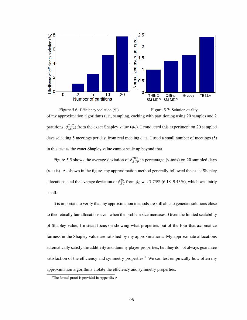
Figure 5.6: Efficiency violation (%) Figure 5.7: Solution quality

of my approximation algorithms (i.e., sampling, caching with partitioning using 20 samples and 2

partitions; φ20,2S CP) from the exact Shapley value (φS ). I conducted this experiment on 20 sampled

days selecting 5 meetings per day, from real meeting data. I used a small number of meetings (5)

in this test as the exact Shapley value cannot scale up beyond that.

Figure 5.5 shows the average deviation of φ20,2S CP in percentage (y-axis) on 20 sampled days

(x-axis). As shown in the figure, my approximation method generally followed the exact Shapley

allocations, and the average deviation of φ20S C from φS was 7.73% (6.18–9.43%), which was fairly

small.

It is important to verify that my approximation methods are still able to generate solutions close

to theoretically fair allocations even when the problem size increases. Given the limited scalability

of Shapley value, I instead focus on showing what properties out of the four that axiomatize

fairness in the Shapley value are satisfied by my approximations. My approximate allocations

automatically satisfy the additivity and dummy player properties, but they do not always guarantee

satisfaction of the efficiency and symmetry properties.5 We can test empirically how often my

approximation algorithms violate the efficiency and symmetry properties.

5The formal proof is provided in Appendix A.

96

Figure 5.6 shows the likelihood that allocations computed from a graph partitions violate

efficiency (in percentage) on the y-axis while varying the number of partitions on the x-axis.

Intuitively, as the number of partitions increases, the likelihood that the efficiency property is

violated also increases. However, the overall likelihood was still less than 8%. In particular, when

5 partitions are used, the likelihood was less than 3%. With respect to the symmetry, the maximum

violation rate was less than 9.2% when the number of partitions varied from 0 to 20. These results

show that my allocations approximately satisfy the properties that axiomatize fairness.

5.3.2 Performance of replanning BM-MDP

In this section, I fist tested if my robust multi-objective MDP algorithm that solves BM-MDPs

could generate robust well-balanced solutions (i.e., lower average regret) as compared to the

standard MDP with a unified reward based on the weighted sum method and the average model

from uncertainty sets, and the pessimistic heuristic for solving BM-MDPs [Kwak et al., 2012a].

The uniform weight distribution was applied to the weighted sum method. 50 different instances

were used.6 Each problem is based on real meeting data. On average, the MDP showed the

worst result among three (2.13 times higher regret than my method) and the pessimistic heuristic

achieved 1.19 times higher regret than mine, which clearly shows that my method is even more

robust than the best known algorithm for solving BM-MDPs.

I then evaluated the performance of the replanning BM-MDP against three approaches while

rescheduling meetings under uncertainty at both planning and execution time: (i) full-online

replanning: it chooses the local best action at every time point (i.e., greedy approach), (ii)

full-offline BM-MDP: it commits to the original policy until completion while ignoring the

6I generate different problem instances while varying the level of uncertainty (0–100%).

97

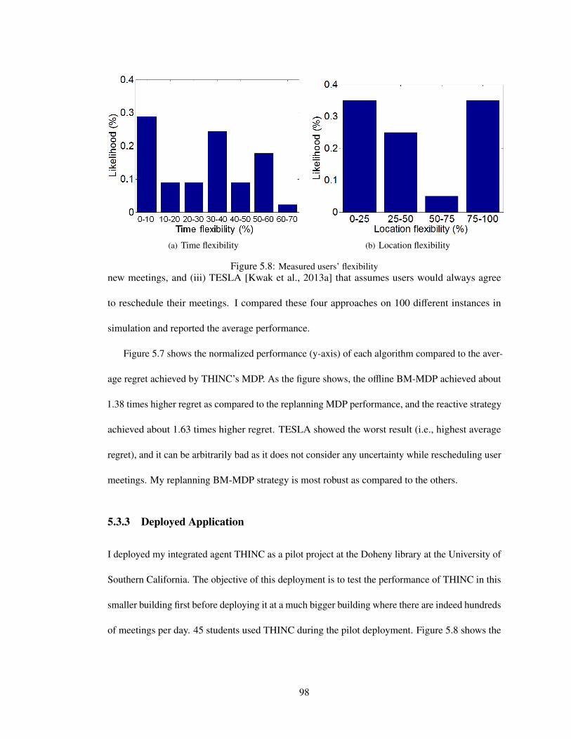
(a) Time flexibility (b) Location flexibility

Figure 5.8: Measured users’ flexibilitynew meetings, and (iii) TESLA [Kwak et al., 2013a] that assumes users would always agree

to reschedule their meetings. I compared these four approaches on 100 different instances in

simulation and reported the average performance.

Figure 5.7 shows the normalized performance (y-axis) of each algorithm compared to the aver-

age regret achieved by THINC’s MDP. As the figure shows, the offline BM-MDP achieved about

1.38 times higher regret as compared to the replanning MDP performance, and the reactive strategy

achieved about 1.63 times higher regret. TESLA showed the worst result (i.e., highest average

regret), and it can be arbitrarily bad as it does not consider any uncertainty while rescheduling user

meetings. My replanning BM-MDP strategy is most robust as compared to the others.

5.3.3 Deployed Application

I deployed my integrated agent THINC as a pilot project at the Doheny library at the University of

Southern California. The objective of this deployment is to test the performance of THINC in this

smaller building first before deploying it at a much bigger building where there are indeed hundreds

of meetings per day. 45 students used THINC during the pilot deployment. Figure 5.8 shows the

98

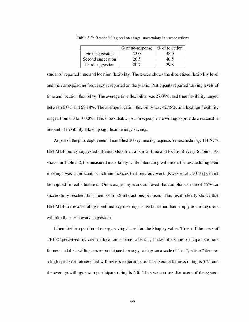
Table 5.2: Rescheduling real meetings: uncertainty in user reactions

% of no-response % of rejectionFirst suggestion 35.0 48.0

Second suggestion 26.5 40.5Third suggestion 20.7 39.8

students’ reported time and location flexibility. The x-axis shows the discretized flexibility level

and the corresponding frequency is reported on the y-axis. Participants reported varying levels of

time and location flexibility. The average time flexibility was 27.05%, and time flexibility ranged

between 0.0% and 68.18%. The average location flexibility was 42.48%, and location flexibility

ranged from 0.0 to 100.0%. This shows that, in practice, people are willing to provide a reasonable

amount of flexibility allowing significant energy savings.

As part of the pilot deployment, I identified 20 key meeting requests for rescheduling. THINC’s

BM-MDP policy suggested different slots (i.e., a pair of time and location) every 6 hours. As

shown in Table 5.2, the measured uncertainty while interacting with users for rescheduling their

meetings was significant, which emphasizes that previous work [Kwak et al., 2013a] cannot

be applied in real situations. On average, my work achieved the compliance rate of 45% for

successfully rescheduling them with 3.6 interactions per user. This result clearly shows that

BM-MDP for rescheduling identified key meetings is useful rather than simply assuming users

will blindly accept every suggestion.

I then divide a portion of energy savings based on the Shapley value. To test if the users of

THINC perceived my credit allocation scheme to be fair, I asked the same participants to rate

fairness and their willingness to participate in energy savings on a scale of 1 to 7, where 7 denotes

a high rating for fairness and willingness to participate. The average fairness rating is 5.24 and

the average willingness to participate rating is 6.0. Thus we can see that users of the system

99

perceive the Shapley based allocation scheme to be highly fair. This average fairness rating is also

consistent with the result from the AMT survey, which further supports the use of Shapley value

as a fair allocation method.

100

Chapter 6: Related Work

Recent years have seen a rise of interest in the development of multiagent systems in energy

domains that inherently have uncertain and dynamic environments with limited resources. In

discussing related work, a key point I wish to emphasize is the uniqueness of my work [Kwak

et al., 2012a,b, 2013a,b] in combining research on multiagent systems, specifically (i) fair division

of credit for energy savings in the context of cooperative game theory; (ii) robust MDP algorithms

that handle multi-objective optimization under uncertainty; and (iii) comfort-based energy-efficient

incremental scheduling in an innovative application for energy savings. It is this specific combi-

nation of attributes that sets my work apart from previous research. Furthermore, a key novelty

as an agent-based system for energy savings is that, my work is evaluated on real building and

meeting/event data that have been collected from more than 500 rooms in ten educational buildings

at USC and SMU.

In this chapter, I will describe research related to my thesis in the following categories: (i)

agent-based systems in energy, (ii) robust MDP and multi-objective techniques, (iii) resource

allocation and scheduling, (iv) fair division in cooperative game theory, and (v) social influence in

human subject studies.

101

6.1 Agent-based Systems in Energy

Agent-based systems have been considered to provide sustainable energy for smart grid manage-

ment. Chalkiadakis et al. [Chalkiadakis et al., 2011] suggested Cooperative Virtual Power Plants

(CVPPs) for achieving the cost-efficient integration of the many distributed energy resources by

relying on a game-theoretic approach. Voice et al. [Voice et al., 2011] provided a game-theoretic

framework for modeling storage devices in large-scale systems where each storage device is owned

by a self-interested agent that aims to maximize its monetary profit. In addition, [Kamboj et al.,

2011] addressed research challenges to integrate plug-in Electric Vehicles (EVs) into the smart

grid. Stein et al. [Stein et al., 2012] also introduced a novel online mechanism that schedules the

allocation of an expiring and continuously-produced resource to self-interested agents with private

preferences while focusing on the fairness using pre-commitment in smart grid domain, which

is not directly applicable in commercial buildings. Miller et al. [Miller et al., 2012] investigated

how the optimal dispatch problem in the smart grid can be framed as a decentralized agent-based

coordination problem and presented a novel decentralized message passing algorithm. Their work

was empirically evaluated in large networks using real distribution network data.

The rise in energy consumption in buildings can be attributed to several factors such as

enhancement of building services and comfort levels [Gao et al., 2010; Perez-Lombard et al.,

2008; Santamouris et al., 1994; Sun and Lee, 2006]. To model and optimize building energy

consumption, Ramchurn et al. [Ramchurn et al., 2011] considered more complex deferrable loads

and managing comfort in the residential buildings. Rogers et al. [Rogers et al., 2011] addressed the

challenge of adaptively controlling a home heating system in order to minimize cost and carbon

emissions within a smart grid using Gaussian processes to predict the environmental parameters.

102

Abras et al. [Abras et al., 2006], Conte et al. [Conte and Scaradozzi, 2003] and Roy et al. [Roy

et al., 2006] have employed multiagent systems to model home automation systems (or smart

homes) and simulating control algorithms to evaluate performance. More recently, Mamidi et

al. [Mamidi et al., 2012b] conducted research on smart sensing and adaptive energy management

system in commercial buildings. They implemented a multi-model sensor agent using various

types of sensors to estimate the number of occupants in each room and predict future occupancy

using machine learning techniques. This prediction can be potentially used for efficient HAVC

operations in the building. Jazizadeh et al. [Jazizadeh et al., 2013a,b] recently focused on building

a human-building interaction framework for understanding personalized thermal comfort models

in office buildings. Research by Li et al. [Li et al., 2012a,b] focused on understanding building

occupancy with RFID on hand-held devices and demand-driven HAVC operations based on the

measured occupancy. My work is different in focusing on energy savings in commercial buildings

by relying on different representation and approaches from previous work, which allows consumers

(i.e., occupants) to play a part in optimizing the operation in the building instead of managing the

optimal demand on buildings.

6.2 Robust MDP and Multi-objective Optimization Techniques

There has been a significant amount of work done on multi-objective optimization. Stadler and

Dauer [Stadler, 1987, 1988; Stadler and Dauer, 1992] provide extensive discussions on the funda-

mental concepts and ideas in this field. In contrast to single-objective optimization, there is no

single global solution while optimizing the multiple criteria, and the most predominant concept in

defining optimal solutions is Pareto Optimality [Pareto, 1906]. Vincent and Grantham [Vincent

103

and Grantham, 1981] and Miettinen [Miettinen, 1999] have been discussing theoretical necessary

and sufficient conditions to formally qualify Pareto Optimality. As alternative to the idea, Saluk-

vadze [Salukvadze, 1971a,b] also proposed a compromised solution concept, which generates a

single solution.

In terms of solution methods, The most common approaches to multi-objective optimization are

to find Pareto optimal solutions by using the weighted sum method to aggregate multiple objectives

using a prior preference [Yoon and Hwang, 1995] or by considering the weighted min-max (or

Tchebycheff ) formulation that provides a nice theoretical property in terms of sufficient/necessary

conditions for Pareto optimality [Koski and Silvennoinen, 1987; Messac et al., 2000a,b; Miettinen,

1999]. It has been proven that if all weight values are positive, this method gives Pareto optimal

solutions [Zadeh, 1963]. However, previous research [Athan and Papalambros, 1996; Das and

Dennis, 1997; Koski, 1985; Messac et al., 2000a,b; Stadler, 1995] discuss about weaknesses of this

method. Despite all these limitations, I use this method as a benchmark method for comparison

purposes since it is still widely used in this field.

Chatterjee et al. [Chatterjee et al., 2006] considered MDPs with multiple discounted reward

objectives. They theoretically analyzed the complexity of the proposed approach and showed that

the Pareto curve can be approximated in polynomial time. Wiering and Jong [Wiering and De Jong,

2007] described a novel algorithm to compute Pareto optimal policies for deterministic multi-

objective sequential decision problems. Authors proved that the algorithm converges to the Pareto

optimal set of value functions and policies for deterministic infinite horizon discounted multi-

objective Markov decision problems. Ogryczak et al. [Ogryczak et al., 2011] focused on finding a

compromise solution in multi-objective MDPs for a well-balanced solution. They compared their

approach relying on the Tchebycheff scalarizing function to the weighted sum method. On the

104

other hand, there has been some significant advances to handle model uncertainty on standard

MDPs including [Delgado et al., 2009; Givan et al., 2000]. Recently, Soh and Demiris [Soh and

Demiris, 2011] extended the previous work and considered the multiple-reward POMDPs. They

presented two hybrid multi-objective evolutionary algorithms that generate non-dominated sets

of policies. My work is different from them as I assume model uncertainty while simultaneously

optimizing multiple criteria in MDPs.

6.3 Resource Allocation and Scheduling

There has been some work focusing on scheduling of home appliances considering user pref-

erences [Bapat et al., 2011; Sou et al., 2011; Xiong et al., 2011]. In particular, they consider

inferred user’s preferred usage profile while scheduling home appliances in residential buildings,

which is considered as a fixed constraint. My work is different as it does not only maximize

energy savings while considering users’ preferences, but also effectively interacts with users to

change their flexibility to achieve further energy savings. More recently, there has been some

work focusing on energy-aware scheduling in commercial buildings [Majumdar et al., 2012]. The

authors only consider the HVAC systems and ignore other significant energy consumers such as

lighting and electronics in commercial buildings while optimizing schedules based on the given

fixed constraints. My thesis work is different by focusing on an energy-oriented scheduling while

considering major energy consumers (HVACs, lighting and electronics) together in commercial

buildings. I also identify key meetings for flexibility change, an aspect that is missing in this

previous work.

105

In a multiagent community, there has been a significant amount of work that has focused

on meeting/event scheduling based on the distributed constraint optimization (DCOP) formu-

lation [Maheswaran et al., 2004; Sultanik et al., 2007]. They provide distributed scheduling

frameworks that are limited to dynamic scheduling problems. In addition, they focused on schedul-

ing meetings without energy considerations. My work differs from their work as it explicitly

aims to conserve energy while scheduling incrementally/dynamically arriving requests. Wainer et

al. [Wainer et al., 2007] also presented a set of protocols for scheduling a meeting among agents

that represent their respective user’s interests and evaluated the suggested protocols while handling

meeting scheduling problems. The objective in their work is to find the optimal protocol to reach

agreement among agents, which does not explicitly account for energy.

Online scheduling techniques have been investigated to handle incremental requests consid-

ering temporal flexibility [Gallagher et al., 2006; Policella et al., 2004]. My work is different by

focusing on energy-oriented scheduling in commercial buildings while allowing people to play a

part in optimizing the operation in the building.

6.4 Fair Division in Cooperative Game Theory

6.4.1 Cooperative Game Theory in Energy Systems

Alam et al. [Alam et al., 2013] investigated the exchange of energy between homes in a community

to reduce the overall battery usage, and showed that agents (acting on the behalf of households)

can coordinate and regulate the exchange of energy between homes which leads to two surpluses:

reduction in the overall battery usage and reduction in the energy losses. To ensure a fair distri-

bution of these surpluses among agents, each agent’s contribution to both surpluses is computed

106

using the Shapley value and an approximation method is used to speed up this computation. Khan

et al. [Khan and Ahmad, 2009] applied the concept of Nash Bargaining Solution (NBS) from co-

operative game theory to minimize energy consumption and response time in computational grids

and showed that the solution is guaranteed to be Pareto-optimal. Zima et al. [Zima-Bockarjova

et al., 2010b] apply cooperative game theoretic concepts to the problem of energy supply system

planning to maximize profit earned by market participants. They find the Shapley value for each

agent to divide additional gains among the coalition participants. Sereno [Sereno, 2012] used

cooperative game theory to develop a framework for energy-aware policies in cellular networks.

[Sereno, 2012] also discusses fair division of benefits derived from cooperating agents based

on the Shapley value solution concept. [Kattuman et al., 2001; Hsieh, 2006; Zima-Bockarjova

et al., 2010a] also discuss the application of Shapley value to solve the loss allocation problem in

electricity markets and for sharing of profit obtained from coordinated operation in hydro and wind

power production domains. My work is different in that it provides an integrated agent that focuses

on fair credit allocations, based on novel efficient Shapley value computation while exploiting the

domain properties. This is for incentivizing users to participate in this energy saving process in

commercial buildings.

6.4.2 Shapley Value and Approximation Techniques

[Bachrach et al., 2013] focuses on showing how various cooperative game-theoretic solution

concepts can be used in a network connectivity scenario (particularly network communication

reliability domain). In particular, they investigated Shapley value, Banzhaf power indices, the

core and the epsilon core. This paper includes a good amount of literature review and polynomial

algorithms for the restricted domain where the graph has a tree structure. Although I construct a

107

flexibility-based influence graph, which is similar to a connectivity graph used in this work, I use a

given general graph mainly for speeding up the computation by considering partitions.

Various methods of approximating the Shapley value can be found in literature. Mann et

al. [Mann and Llyod, 1960] proposed a Monte-Carlo simulation technique for approximating the

Shapley value and applied it to analyze the US electoral-voting system. Owen’s [Owen, 1972]

multilinear extension method for approximating the Shapley value in weighted voting games is

linear in the number of players. Fatima et al. [Fatima et al., 2008] also provided an approximation

method for the Shapley value which is linear in the number of players for k-majority games.

However, the approximation error for their method was relatively low as compared to Owen’s.

They also empirically evaluated the approximation error and analyzed how various parameters of

a voting game, like the number of players and the quota, affect the error. Aadithya et al. [Aadithya

et al., 2010] explored efficient ways of calculating the Shapley value for network centralities.

Besides deriving closed-form expressions for the Shapley values based on the underlying network

structure and the game defined over the network, they also provide exact and polynomial time

Shapley value approximation algorithms based on them. Bachrach et al. [Bachrach et al., 2010]

includes a thorough literature survey of methods to approximate power indices such as the Banzhaf

and Shapley-Shubik power indices. They also suggest and analyze approximation algorithms for

these power indices and provide lower bounds for both deterministic and randomized algorithms

to calculate these indices. They also noted that the Shapley-Shubik power index approximation

method suggested in [Bachrach et al., 2010] can be adapted to efficiently compute the Shapley

value by using proper bounds for the Hoeffding inequality and thus use it to compute an individual’s

relative contribution to the IQ of a group in [Bachrach et al., 2012]. My approximation technique is

different from previous work as I exploit domain properties to integrate a novel graph partitioning

108

algorithm, caching technique, and an LP relaxation method to approximate the Shapley value and

simultaneously speed up its computation. In addition, my work integrates this technique within an

agent that (re)schedules meetings.

6.5 Social Influence in Human Subject Studies

I leverage lessons and insights from social psychology in understanding and designing reliable

and accurate human behavior models to compute robust strategies in the real-world. Wood and

Neal [Wood and Neal, 2007, 2009] have studied the potential of interventions to reduce energy

consumption and they have shown that it is not only to change workplace energy consumption

but also to establish energy use habits that maintain over time. Abrahmase et al. [Abrahmase

et al., 2005] reviewed 38 interventions aimed to reduce household energy consumption, and

they showed that information campaigns often improve knowledge but have limited influence

on behavior or energy savings in residential buildings. According to their study, when monetary

rewards were given for energy savings, energy consumption decreased in the short-run but not in

the longer-term after the rewards were terminated, and they concluded that normative feedback

about energy use is the most promising strategy for reducing and maintaining low consumption.

However, it focused on residential environments, which is different from my work. In a recent

study, Carrico and Riemer [Carrico and Riemer, 2011] provided monthly normative feedback via

email to occupants of a commercial building about their own buildings’ energy use in comparison

with and other, similar buildings. Unfortunately, the study only relied on self-reporting to assess

the behaviors. Instead, my work relies on both real sensors to observe their energy behavior in

real-time and self-reporting. Faruqui et al. [Faruqui et al., 2010] reviewed past experiments and

109

pilot projects to evaluate the effect of in-home displays (IHDs) on energy consumption. My work

is different because I simultaneously consider multiple criteria including energy consumption and

occupant comfort level. Research by Fahrioglu et al. [Fahrioglu and Alvardo, 2000], Mohsenian-

Rad et al. [Mohsenian-Rad et al., 2010] and Caron et al. [Caron and Kesidis, 2010] provide

incentive compatible mechanisms for distribution of energy among interested parties. This thread

of research is complementary, especially in designing incentives for humans to reveal their true

energy preferences. However, these approaches assume a centralized controller with whom all the

members interact, which is not present in my domain. Instead, there are peer-to-peer negotiations

between humans regarding their energy consumption and comfort level.

In social psychology, there has been a significant deal of work to figure out the correlation

between irritation/distraction factors and persuasion. McCullough and Ostrom [McCullough and

Ostrom, 1974], Cacioppo and Petty [Cacioppo and Petty, 1989] and Nordhielm [Nordhielm, 2002]

discussed that message repetition would increase positive attitudes in a situation where highly

similar communications are used and showed that there is a positive relationship between the

number of presentations and attitude from general social psychology perspectives. Focusing on a

commercial advertisement, Pechmann and Stewart [Pechmann and Stewart, 1988], Schumann et

al. [Schumann et al., 1990] and Calder and Sternthal [Calder and Sternthal, 1980] predicted the

effectiveness of different strategies on advertising and examined the effects of message repetition

on attitude changes. In addition, Baron et al. [Baron et al., 1973], Bither [Bither, 1972] and Regan

and Cheng [Regan and Cheng, 1973] discussed that distractions affect behavior decisions, but

they are more or less effective in increasing persuasion depending upon whether people can easily

ignore the distraction.

110

Chapter 7: Conclusions

The rapid growth in energy usage has made the need for systems that aid in reducing energy

consumption a top priority. To that end, researchers in multiagent community have been developing

multiagent systems to conserve energy for deployment in the smart grid and buildings [Kamboj

et al., 2011; Mamidi et al., 2012a; Miller et al., 2012; Ramchurn et al., 2011; Rogers et al., 2011;

Gerding et al., 2011; Chalkiadakis et al., 2011; Voice et al., 2011]. Despite the recent success to

forge a new area of agent-based systems for energy conservation, their work has been done with a

particular focus on residential buildings, and does not directly apply to commercial buildings. For

successfully developing real-world energy systems to conserve energy in commercial buildings,

three unique research challenges should be simultaneously addressed. First, algorithms should

be able to handle massive meetings/events schedules while focusing on conserving energy and

considering the given human models. Second, there are different types of energy-related behaviors

in commercial buildings from residential ones. They require agents to negotiate with groups of

people for guiding their behaviors to conserve energy while ensuring a balance of energy savings

and comfort under uncertainty over people’s behavior preferences. Third, the systems should

also ensure that proper credit is given based on people’s true contribution in energy savings for

effectively motivating people.

111

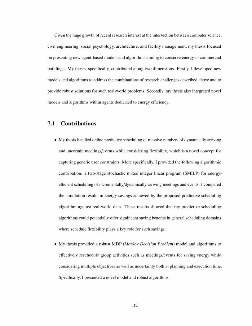
Given the huge growth of recent research interest at the intersection between computer science,

civil engineering, social psychology, architecture, and facility management, my thesis focused

on presenting new agent-based models and algorithms aiming to conserve energy in commercial

buildings. My thesis, specifically, contributed along two dimensions. Firstly, I developed new

models and algorithms to address the combinations of research challenges described above and to

provide robust solutions for such real-world problems. Secondly, my thesis also integrated novel

models and algorithms within agents dedicated to energy efficiency.

7.1 Contributions

• My thesis handled online predictive scheduling of massive numbers of dynamically arriving

and uncertain meetings/events while considering flexibility, which is a novel concept for

capturing generic user constraints. More specifically, I provided the following algorithmic

contribution: a two-stage stochastic mixed integer linear program (SMILP) for energy-

efficient scheduling of incrementally/dynamically arriving meetings and events. I compared

the simulation results in energy savings achieved by the proposed predictive scheduling

algorithm against real-world data. These results showed that my predictive scheduling

algorithms could potentially offer significant saving benefits in general scheduling domains

where schedule flexibility plays a key role for such savings.

• My thesis provided a robust MDP (Markov Decision Problem) model and algorithms to

effectively reschedule group activities such as meetings/events for saving energy while

considering multiple objectives as well as uncertainty both at planning and execution time.

Specifically, I presented a novel model and robust algorithms:

112

– BM-MDP (Bounded-parameter Multi-objective MDP) that explicitly models multiple

criteria as well as uncertainty over people’s preferences

– robust algorithms to solve BM-MDPs and dynamic replanning methods for handling

uncertainty at execution time

I showed that BM-MDPs with replanning generated robust solutions while considering

multiple criteria and model uncertainty at both planning and execution time.

• My thesis addressed fair division of credit using concepts of cooperative game theory. In

particular, I appealed to cooperative game theory and specifically to the concept of Shapley

value for this fair division. Unfortunately, scaling up this Shapley value computation is a

major hindrance in practice. Therefore, I presented a novel algorithmic contribution for

scaling up the overall computations:

– approximation algorithms to efficiently compute the Shapley value based on sampling

and partitions

– an LP (linear program) relaxation method to speed up the characteristic function

computation

These approximations allowed efficient computations of fair individual allocations in a

large-scale saving game in the real-world. I also showed that different combinations of these

approximations can be chosen under particular circumstances while considering the tradeoff

between solution quality and runtime.

• My algorithmic contributions have been successfully integrated within agents dedicated to

energy efficiency: SAVES, TESLA and THINC. SAVES provided several key novelties:

113

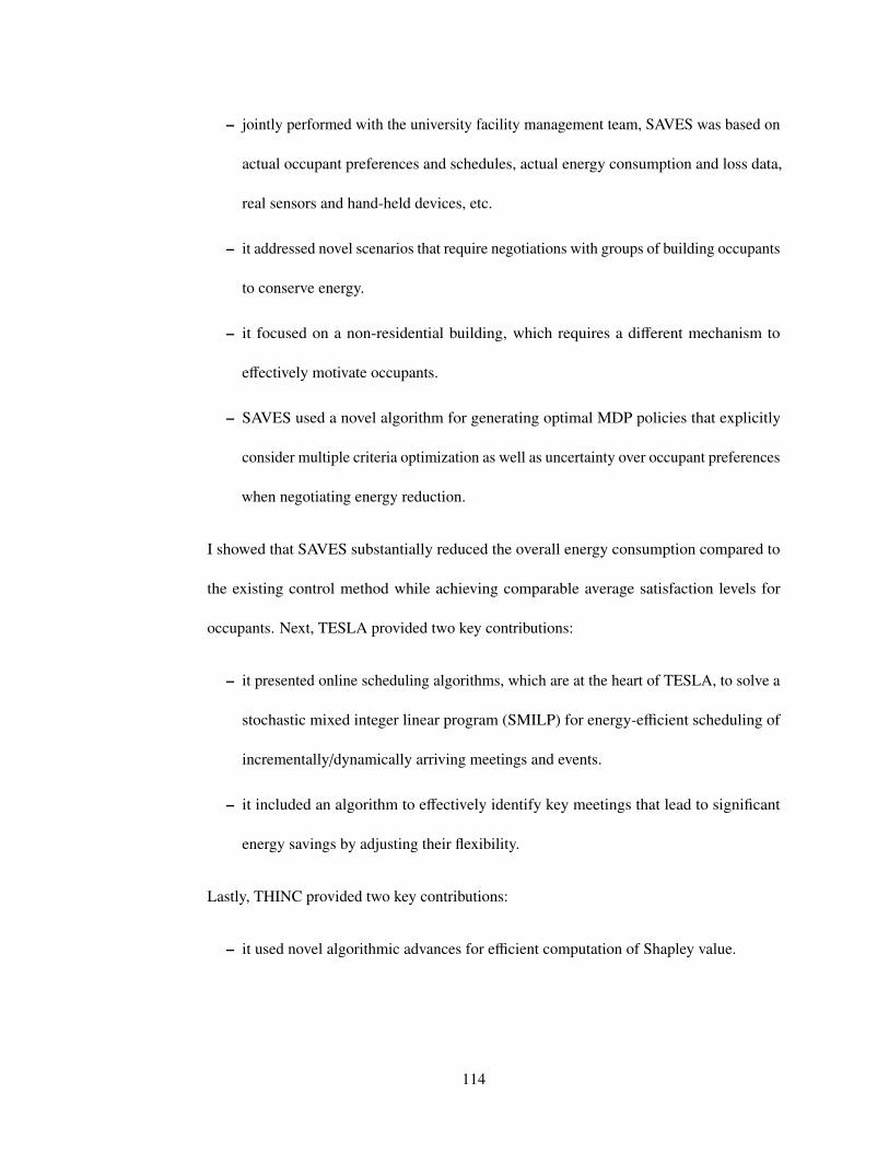
– jointly performed with the university facility management team, SAVES was based on

actual occupant preferences and schedules, actual energy consumption and loss data,

real sensors and hand-held devices, etc.

– it addressed novel scenarios that require negotiations with groups of building occupants

to conserve energy.

– it focused on a non-residential building, which requires a different mechanism to

effectively motivate occupants.

– SAVES used a novel algorithm for generating optimal MDP policies that explicitly

consider multiple criteria optimization as well as uncertainty over occupant preferences

when negotiating energy reduction.

I showed that SAVES substantially reduced the overall energy consumption compared to

the existing control method while achieving comparable average satisfaction levels for

occupants. Next, TESLA provided two key contributions:

– it presented online scheduling algorithms, which are at the heart of TESLA, to solve a

stochastic mixed integer linear program (SMILP) for energy-efficient scheduling of

incrementally/dynamically arriving meetings and events.

– it included an algorithm to effectively identify key meetings that lead to significant

energy savings by adjusting their flexibility.

Lastly, THINC provided two key contributions:

– it used novel algorithmic advances for efficient computation of Shapley value.

114

– it included a novel robust algorithm to optimally reschedule identified key meetings

addressing user interaction uncertainty.

TESLA and THINC were evaluated on data gathered from over 110,000 meetings held at

nine campus buildings during an eight month period in 2011–2012 at USC and SMU. These

results and analysis showed that, compared to the current systems, they could substantially

reduce overall energy consumption. In addition, Finally, THINC was deployed in the real-

world as a pilot project at the Doheny library at USC and presented results illustrating the

benefits in saving energy.

7.2 Future Work

As described in the earlier section, my work provided three key algorithmic contributions in-

cluding (i) energy-efficient scheduling of user meeting requests while considering flexibility, (ii)

rescheduling of key energy-consuming meetings for more energy savings, and (iii) efficient fair

credit allocations based on Shapley value to incentivize users for their energy saving activities.

These new models and methods have not only advanced the state of the art in multiagent algo-

rithms, but have actually been successfully integrated within agents dedicated to energy efficiency,

clearly demonstrating the potential of agent technology to assist human users in saving energy in

commercial buildings.

However, there exist some remaining open challenges which can be explored for building

real-world energy applications going forward:

• My present dynamic replanning MDP methods provide a reasonable way to handle uncer-

tainty both at planning and execution time; however, the further investigation regarding the

115

trigger points deciding when to keep the existing policy or when to regenerate the policy

from the scratch.

• Scalability could be further investigated to further speed up the characteristic function

computation by adopting the decomposition methods such as a Lagrangian decomposition.

• Although real building data of the Leavey library including the actual floor flan, lighting

specifications, etc., were used, the energy consumption validation on the library building

has not been thoroughly conducted in the simulation environment.1

• In practice, it is challenging to know the exact human behavior models while interacting

with users to reschedule their activities under different circumstances. So far, in this work, I

relied on sparse samples from surveys (conducted in RGL and Amazon Mechanical Turk

(AMT)) to construct the behavior models and applied the same models to different buildings

(e.g., Leavey and Doheny libraries), which results in potential noises on results.

• Human subject experiments were conducted in a limited fashion:

– AMT, which I have used for conducting human subject experiments, is limited to

provide participants with the exact context in detail as it often assumes hypothetical

situations which might not be realized in practice.

– The human subject experiments conducted at USC with staff and students relied upon

self-reports which may not reflect actual circumstances, and long-term effects were

not observed.1The energy consumption validation has been thoroughly performed on the RGL building while ignoring the heat

transfer effect between spaces for HVACs.

116

– Human subject experiments were conducted under a specifically controlled environ-

ment, which may result in biased results from human participants.

• Although the Shapley value has been widely adopted for mathematically computing fair

individual allocations, human conceptions of its fairness to actual users in my domain have

not yet been explored.

• The proposed algorithms were mainly evaluated in simulation, and the integrated agent has

been only deployed at the Doheny library as a pilot project in a limited fashion. Although the

simulation results clearly support the argument that the proposed methods have significant

potential in saving energy, the full-scale deployment will be eventually required to verify

the end-to-end operations of my agent in real commercial buildings.

• So far, the effects of social norm-based feedback and monetary-based feedback on changing

people’s (habitual) behaviors have not been investigated thoroughly in this energy domain.

• The social norm-based feedback on groups of human users has not been explored in my

work.

117

Bibliography

Karthik V. Aadithya, Balaraman Ravindran, Tomasz P. Michalak, and Nicholas R. Jennings.Efficient computation of the shapley value for centrality in networks. In Proceedings of the 6thinternational conference on Internet and network economics, WINE’10, pages 1–13, Berlin,Heidelberg, 2010. Springer-Verlag.

W. Abrahmase, L. Steg, C. Vlek, and T. Rothengatter. A review of intervention studies aimed athousehold energy conservation. J Environ. Psychol., 25:273–291, 2005.

S. Abras, S. Ploix, S. Pesty, and M. Jacomino. A multi–agent home automation system for powermanagement. In ICINCO, 2006.

S. Abras, S. Ploix, S. Pesty, and M. Jacomino. A multi-agent home automation system for powermanagement. Informatics in Control Automation and Robotics, 15:59–68, 2008.

Shabbir Ahmed, Alexander Shapiro, and Er Shapiro. The sample average approximation methodfor stochastic programs with integer recourse. SIAM Journal of Optimization, 12:479–502,2002.

Muddasser Alam, Sarvapali D Ramchurn, and Alex Rogers. Cooperative energy exchange forthe efficient use of energy and resources in remote communities. In Proceedings of the 2013international conference on Autonomous agents and multi-agent systems, pages 731–738.International Foundation for Autonomous Agents and Multiagent Systems, 2013.

David Aldous. Exchangeability and related topics. Ecole d’Ete de Probabilites de Saint-FlourXIII?1983, pages 1–198, 1985.

K. Anderson, S. Lee, and C. Menassa. Effect of social network type on building occupant energyuse. In Buildsys, pages 17–24. ACM, 2012.

T.W. Athan and P.Y. Papalambros. A note on weighted criteria methods for compromise solutionsin multi-objective optimization. Eng. Optim., 27:155–176, 1996.

Yoram Bachrach, Evangelos Markakis, Ezra Resnick, Ariel D. Procaccia, Jeffrey S. Rosenschein,and Amin Saberi. Approximating power indices: theoretical and empirical analysis. AutonomousAgents and Multi-Agent Systems, 20(2):105–122, March 2010. ISSN 1387-2532.

Yoram Bachrach, Thore Graepel, Gjergji Kasneci, Michal Kosinski, and Jurgen Van Gael. Crowdiq: aggregating opinions to boost performance. In Proceedings of the 11th InternationalConference on Autonomous Agents and Multiagent Systems - Volume 1, AAMAS ’12, pages535–542, Richland, SC, 2012. International Foundation for Autonomous Agents and MultiagentSystems. ISBN 0-9817381-1-7, 978-0-9817381-1-6.

118

Yoram Bachrach, Ely Porat, and Jeffrey S Rosenschein. Sharing rewards in cooperative connectivitygames. Journal of Artificial Intelligence Research, 47:281–311, 2013.

James Bagnell, Andrew Y Ng, and Jeff Schneider. Solving uncertain markov decision problems.Robotics Institute, Carnegie Mellon University, Pittsburgh, PA, Tech. Rep. CMU-RI-TR-01-25,2001.

Tanuja Bapat, Neha Sengupta, Sunil K. Ghai, Vijay Arya, Yedendra B. Shrinivasan, and DevaSeetharam. User-sensitive scheduling of home appliances. In SIGCOMM, 2011.

R.S. Baron, P.H. Baron, and N. Miller. The relation between distraction and persuasion. Psycho-logical Bulletin, 80(4):310, 1973.

EML Beale. On minimizing a convex function subject to linear inequalities. Journal of the RoyalStatistical Society. Series B (Methodological), pages 173–184, 1955.

S.W. Bither. Effects of distraction and commitment on the persuasiveness of television advertising.Journal of Marketing Research, pages 1–5, 1972.

J.T. Cacioppo and R.E. Petty. Effects of message repetition on argument processing, recall, andpersuasion. Basic and Applied Social Psychology, 10(1):3–12, 1989.

B.J. Calder and B. Sternthal. Television commercial wearout: An information processing view.Journal of Marketing Research, pages 173–186, 1980.

S. Caron and G. Kesidis. Incentive-based energy consumption scheduling algorithms for the smartgrid. In SmartGridComm, 2010.

A.R. Carrico and M. Riemer. Motivating energy conservation in the workplace: An evaluation ofthe use of group-level feedback and peer education. J Environ. Psychol., 31, 2011.

Javier Castro, Daniel Gomez, and Juan Tejada. Polynomial calculation of the shapley value basedon sampling. Computers & Operations Research, 36(5):1726–1730, 2009.

Georgios Chalkiadakis, Valentin Robu, Ramachandra Kota, Alex Rogers, and Nick Jennings.Cooperatives of distributed energy resources for efficient virtual power plants. In AAMAS, 2011.URL http://eprints.ecs.soton.ac.uk/21950/.

Krishnendu Chatterjee, Rupak Majumdar, and Thomas A. Henzinger. Markov decision processeswith multiple objectives. In STACS, 2006.

G. Conte and D. Scaradozzi. Viewing home automation systems as multiple agents systems. InMulti-agent system for industrial and service robotics applications, RoboCUP, 2003.

George B Dantzig. Linear programming under uncertainty. Management Science, 1(3-4):197–206,1955.

I. Das and J.E. Dennis. A closer look at drawbacks of minimizing weighted sums of objectives forpareto set generation in multicriteria optimization problems. Struct. Optim., 14:63–69, 1997.

119

Karina Valdivia Delgado, Scott Sanner, Leliane Nunes de Barros, and Fabio G. Cozman. Efficientsolutions to factored MDPs with imprecise transition probabilities. In AAAI, 2009.

M. Fahrioglu and F. L. Alvardo. Designing incentive compatible contracts for effective demandmanagements. IEEE Trans. Power Systems, 15:1255–1260, 2000.

Ahmad Faruqui, Sanem Sergici, and Ahmed Sharif. The impact of informational feedback onenergy consumption - a survey of the experimental evidence. Energy, 35, 2010.

Shaheen S. Fatima, Michael Wooldridge, and Nicholas R. Jennings. A linear approximationmethod for the shapley value. Artif. Intell., 172(14):1673–1699, September 2008. ISSN0004-3702.

A. Gallagher, T. Zimmerman, and S. Smith. Incremental scheduling to maximize quality in adynamic environment. In ICAPS, 2006.

Y. Gao, E. Tumwesigye, B. Cahill, and K. Menzel. Using data mining in optimization of buildingenergy consumption and thermal comfort management. In SEDM, 2010.

Enrico Gerding, Valentin Robu, Sebastian Stein, David Parkes, Alex Rogers, and Nick Jennings.Online mechanism design for electric vehicle charging. In AAMAS, 2011. URL http://eprints.ecs.soton.ac.uk/21907/.

Donald B Gillies. Solutions to general non-zero-sum games. Contributions to the Theory ofGames, 4:47–85, 1959.

Robert Givan, Sonia Leach, and Thomas Dean. Bounded-parameter Markov decision processes.Artificial Intelligence, 2000.

Gerard Hamiache. Associated consistency and shapley value. International Journal of GameTheory, 30(2):279–289, 2001.

Kevin A Hassett and Gilbert E Metcalf. Energy tax credits and residential conservation investment:Evidence from panel data. Journal of Public Economics, 57(2):201–217, 1995.

Shih-Chieh Hsieh. Fair transmission loss allocation based on equivalent current injection andshapley value. In IEEE Power Engineering Society General Meeting, pages 6 pp.–, 2006.

F. Jazizadeh, A. Ghahramani, B. Becerik-Gerber, T. Kichkaylo, and M. Orosz. A human-building interaction framework for personalized thermal comfort driven systems in officebuildings. Journal of Computing in Civil Engineering, 2013a. doi: 10.1061/(ASCE)CP.1943-5487.0000300. URL http://ascelibrary.org/doi/abs/10.1061/%28ASCE%29CP.1943-5487.0000300.

Farrokh Jazizadeh, Geoffrey Kavulya, Laura Klein, and Burcin Becerik-Gerber. Continuoussensing of occupant perception of indoor ambient factors. In ASCE International Workshop onComputing in Civil Engineering, 2011.

Farrokh Jazizadeh, Franco Moiso Marin, and Burcin Becerik-Gerber. A thermal preferencescale for personalized comfort profile identification via participatory sensing. Building andEnvironment, 2013b.

120

Peter Kall and Stein W Wallace. Stochastic programming. John Wiley and Sons Ltd, 1994.

S. Kamboj, W. Kempton, and K. S. Decker. Deploying power grid-integrated electric vehicles as amulti-agent system. In AAMAS, 2011.

P.A. Kattuman, R.J. Green, and J.W. Bialek. A tracing method for pricing inter-area electric-ity trades. Cambridge working papers in economics, Faculty of Economics, University ofCambridge, June 2001.

H. Ezzat Khalifa, Can Isik, and John F. III Dannenhoffer. Energy efficiency of distributedenvironmental control systems. Technical Report DOE-ER63694-1, Syracuse Univ., 2006.

Samee U. Khan and Ishfaq Ahmad. A cooperative game theoretical technique for joint optimizationof energy consumption and response time in computational grids. IEEE Trans. Parallel Distrib.Syst., 20(3):346–360, March 2009. ISSN 1045-9219.

J. Koski. Defectiveness of weighting method in multi-criterion optimization of structures. Commun.Appl. Numer. Methods, 1:333–337, 1985.

J. Koski and R. Silvennoinen. Norm methods and partial weighting in multicriterion optimizationof structures. Int. J. Numer. Methods Eng., 24:1101–1121, 1987.

Jun-young Kwak, Pradeep Varakantham, Rajiv Maheswaran, Milind Tambe, Farrokh Jazizadeh,Geoffrey Kavulya, Laura Klein, Burcin Becerik-Gerber, Timothy Hayes, and Wendy Wood.SAVES: A sustainable multiagent application to conserve building energy considering occupants.In AAMAS, 2012a.

Jun-young Kwak, Pradeep Varakantham, Rajiv Maheswaran, Milind Tambe, Farrokh Jazizadeh,Geoffrey Kavulya, Laura Klein, Burcin Becerik-Gerber, Timothy Hayes, and Wendy Wood. Sus-tainable multiagent application to conserve energy. In International Conference on AutonomousAgents and Multiagent Systems (AAMAS) Demonstration Track, 2012b.

Jun-young Kwak, Pradeep Varakantham, Rajiv Maheswaran, Yu-Han Chang, Milind Tambe,Burcin Becerik-Gerber, and Wendy Wood. TESLA: An extended study of an energy-savingagent that leverages schedule flexibility. Journal of Autonomous Agents and Multiagent Systems(JAAMAS), 2013a.

Jun-young Kwak, Pradeep Varakantham, Rajiv Maheswaran, Yu-Han Chang, Milind Tambe,Burcin Becerik-Gerber, and Wendy Wood. Tesla: An energy-saving agent that leveragesschedule flexibility. In International Conference on Autonomous Agents and Multiagent Systems(AAMAS), 2013b.

Kevin Leyton-Brown and Yoav Shoham. Essentials of game theory: A concise multidisciplinaryintroduction. Synthesis Lectures on Artificial Intelligence and Machine Learning, 2(1):1–88,2008.

N. Li, G. Calis, and B. Becerik-Gerber. Measuring and monitoring occupancy with an RFID basedsystem for demand-driven HVAC operations. Journal of Automation in Construction, 24:89–99,2012a.

121

N. Li, S. Li, B. Becerik-Gerber, and G. Calis. Deployment strategies and performance evaluationof a virtual-tag-enabled indoor localization approach. ASCE Journal of Computing in CivilEngineering, 26(5):574–583, 2012b.

Rajiv T Maheswaran, Milind Tambe, Emma Bowring, Jonathan P Pearce, and Pradeep Varakan-tham. Taking dcop to the real world: Efficient complete solutions for distributed multi-eventscheduling. In Proceedings of the Third International Joint Conference on Autonomous Agentsand Multiagent Systems-Volume 1, pages 310–317. IEEE Computer Society, 2004.

A. Majumdar, D. H. Albonesi, and P. Bose. Energy-aware meeting scheduling algorithms forsmart buildings. In Buildsys, pages 161–168. ACM, 2012.

Sunil Mamidi, Yu-Han Chang, and Rajiv Maheswaran. Improving building energy efficiency witha network of sensing, learning and prediction agents. In AAMAS, 2012a.

Sunil Mamidi, Yu-Han Chang, and Rajiv Maheswaran. Improving building energy efficiencywith a network of sensing, learning and prediction agents. In AAMAS, 2012b. URL http://cbg.isi.edu/wp-content/uploads/publications/3.pdf.

Irwin Mann and Shapley S. Llyod. Values of large games, iv: Evaluating the electoral college bymonte-carlo techniques. Technical report, The Rand Corporation, Santa Monica, CA, USA,1960.

J.L. McCullough and T.M. Ostrom. Repetition of highly similar messages and attitude change.Journal of Applied Psychology, 59(3):395, 1974.

A. Messac, C.P. Sukam, and E. Melachrinoudis. Aggregate objective functions and Pareto frontiers:required relationships and practical implications. Optim. Eng., 1:171–188, 2000a.

A. Messac, G.J. Sundararaj, R.V. Tappeta, and J.E. Renaud. Ability of objective functions togenerate points on nonconvex pareto frontiers. AIAA Journal, 38:1084–1091, 2000b.

K. Miettinen. Nonlinear Multiobjective Optimization. Kluwer Academic Publishers, 1999.

Sam Miller, Sarvapali D. Ramchurn, and Alex Rogers. Optimal decentralised dispatch of embeddedgeneration in the smart grid. In AAMAS, 2012.

ZhengChun Mo and Ardeshir Mahdavi. An agent-based simulation-assisted approach to bi-lateralbuilding systems control. In IBPSA, 2003.

A.-H. Mohsenian-Rad and A. Leon-Garcia. Optimal residential load control with price predictionin real-time electricity pricing environments. Smart Grid, IEEE Transaction on, 1(2):120–133,2010.

A.-H. Mohsenian-Rad, V.W.S. Wong, J. Jatskevich, and R. Schober. Optimal and autonomousincentivebased energy consumption scheduling algorithm for smart grid. In ISGT, 2010.

Mahesh Nagarajan, Greys Sosic, and Hao Zhang. Stable group purchasing organizations. MarshallSchool of Business Working Paper No. FBE, pages 20–10, 2010.

Noam Nisan. Algorithmic game theory. Cambridge University Press, 2007.

122

C.L. Nordhielm. The influence of level of processing on advertising repetition effects. Journal ofconsumer research, 29(3):371–382, 2002.

Wlodzimierz Ogryczak, Patrice Perny, and Paul Weng. A compromise programming approach tomultiobjective Markov decision processes. In MCDM, 2011.

A. Osyczka. An approach to multicriterion optimization problems for engineering design. Comput.Methods Appl. Mech. Eng., 15:309–333, 1978.

Guillermo Owen. Multilinear extensions of games. Management Science, 18(5):64–79, January1972. ISSN 0004-3702.

BK Pagnoncelli, S Ahmed, and A Shapiro. Sample average approximation method for chance con-strained programming: theory and applications. Journal of optimization theory and applications,142(2):399–416, 2009.

V. Pareto. Manuale di Economica Politica. Societa Editrice Libraria, 1906.

C. Pechmann and D.W. Stewart. Advertising repetition: A critical review of wearin and wearout.Current issues and research in advertising, 1988.

L. Perez-Lombard, J. Ortiz, and C. Pout. A review on buildings energy consumption information.Energy and Buildings, 40:394–398, 2008.

N. Policella, S. F. Smith, A. Cesta, and A. Oddi. Incremental scheduling to maximize quality in adynamic environment. In ICAPS, 2004.

Martin L Puterman. Markov decision processes: discrete stochastic dynamic programming, volume414. Wiley. com, 2009.

S. D. Ramchurn, P. Vytelingum, A. Rogers, and N. R. Jennings. Agent-based control for decen-tralised demand side management in the smart grid. In AAMAS, 2011.

D.T. Regan and J.B. Cheng. Distraction and attitude change: A resolution. Journal of ExperimentalSocial Psychology, 9(2):138–147, 1973.

Alex Rogers, Sasan Maleki, Siddhartha Ghosh, and Nicholas Jennings. Adaptive home heatingcontrol through Gaussian process prediction and mathematical programming. In InternationalWorkshop on Agent Technology for Energy Systems (ATES), 2011. URL http://eprints.ecs.soton.ac.uk/22235/.

Nirmalya Roy, Abhishek Roy, and Sajal K. Das. Context-aware resource management in multi-inhabitant smart homes: A nash h-learning based approach. In PerCom, 2006. ISBN 0-7695-2518-0. doi: 10.1109/PERCOM.2006.18. URL http://portal.acm.org/citation.cfm?id=1128015.1128338.

M.E. Salukvadze. Optimization of vector functionals, I, programming of optimal trajectories.Avtomatika i Telemekhanika, 8:5–15, 1971a.

M.E. Salukvadze. Optimization of vector functionals, II, the analytic construction of optimalcontrols. Avtomatika i Telemekhanika, 9:5–15, 1971b.

123

M. Santamouris, A. Argiriou, E. Dascalaki, C. Balaras, and A. Gaglia. Energy characteristics andsavings potential in office buildings. Solar Energy, 52:59–66, 1994.

Paul Scerri, David V. Pynadath, and Milind Tambe. Towards adjustable autonomy for the realworld. JAIR, 17:171–228, 2002.

David Schmeidler. The nucleolus of a characteristic function game. SIAM Journal on appliedmathematics, 17(6):1163–1170, 1969.

D.W. Schumann, R.E. Petty, and D.S. Clemons. Predicting the effectiveness of different strategiesof advertising variation: A test of the repetition-variation hypotheses. Journal of ConsumerResearch, pages 192–202, 1990.

Nathan Schurr, Janusz Marecki, and Milind Tambe. Improving adjustable autonomy strategies fortime-critical domains. In AAMAS, 2009.

Matteo Sereno. Cooperative game theory framework for energy efficient policies in wirelessnetworks. In Proceedings of the 3rd International Conference on Future Energy Systems: WhereEnergy, Computing and Communication Meet, e-Energy ’12, pages 17:1–17:9, New York, NY,USA, 2012. ACM.

Alexander Shapiro, Darinka Dentcheva, and Andrzej Ruszczynski. Lectures on stochastic pro-gramming: modeling and theory, volume 9. Society for Industrial Mathematics, 2009.

Lloyd S. Shapley. A value for n-person games. Kuhn HW, Tucker AW, editors. Contributions to thetheory of games II, Annals of mathematics studies, 28:307–317, 1953.

H. Soh and Y. Demiris. Evolving policies for multi-reward partially observable markov deci-sion processes (mr-pomdps). In Proceedings of the 13th annual conference on Genetic andevolutionary computation, pages 713–720. ACM, 2011.

Kin Cheong Sou, James Weimer, Henrik Sandberg, and Karl Henrik Johansson. Scheduling smarthome appliances using mixed integer linear programming. In CDC-ECC, 2011.

W. Stadler. Initiators of multicriteria optimization. Recent Advances and Historical Developmentof Vector Optimization, 294:3–25, 1987.

W. Stadler. Fundamentals of multicriteria optimization. Multicriteria Optimization in Engineeringand in the Sciences, pages 1–25, 1988.

W. Stadler. Caveats and boons of multicriteria optimization. Microcomput. Civ. Eng., 10:291–299,1995.

W. Stadler and J.P. Dauer. Multicriteria optimization in engineering: a tutorial and survey.Structural Optimization: Status and Promise, pages 211–249, 1992.

ASHRAE Standard. Standard 62-2001, ventilation for acceptable indoor air quality. AmericanSociety of Heating, Refrigerating, and Air-Conditioning Engineers, Atlanta, www. ASHRAE.org, 2001.

124

Sebastian Stein, Enrico Gerding, Valentin Robu, and Nick Jennings. A model-based onlinemechanism with pre-commitment and its application to electric vehicle charging. In AAMAS,2012. URL http://eprints.soton.ac.uk/273082/.

Evan Sultanik, Pragnesh Jay Modi, and William C Regli. On modeling multiagent task schedulingas a distributed constraint optimization problem. In Proceedings of the 20th International JointConference on Artificial Intelligence, pages 1531–1536, 2007.

H. S. Sun and S. E. Lee. Case study of data centers’ energy performance. Energy and Buildings,38:522–533, 2006.

U.S. Department of Energy. Buildings energy data book. http://buildingsdatabook.eren.doe.gov/, 2010.

U.S. Department of Labor. Average energy prices in the Los Angeles area. http://www.bls.gov/ro9/cpilosa_energy.htm, 2012.

Stijn Vandael, Klaas De Craemer, Nelis Boucke, Tom Holvoet, and Geert Deconinck. Decentralizedbalancing of a commercial portfolio with plug-in hybrid vehicles in a smart grid. In AAMAS,2011.

T.L. Vincent and W.J. Grantham. Optimality in Parametric Systems. John Wiley & Sons, 1981.

Thomas Voice, Perukrishnen Vytelingum, Sarvapali Ramchurn, Alex Rogers, and Nick Jennings.Decentralised control of micro-storage in the smart grid. In AAAI, 2011. URL http://eprints.ecs.soton.ac.uk/22262/.

P. Vytelingum, T. D. Voice, S. D. Ramchurn, A. Rogers, and N. R. Jennings. Agent-basedmicro-storage management for the smart grid. In AAMAS, 2010.

Jacques Wainer, Paulo Roberto Ferreira Jr., and Everton Rufino Constantino. Scheduling meetingsthrough multi-agent negotiations. Decision Support Systems, 44(1), 2007.

Chen Wang, M. de Groot, and P. Marendy. A service-oriented system for optimizing residentialenergy use. In Web Services, IEEE International Conference on, 2009.

M.A. Wiering and E.D. De Jong. Computing optimal stationary policies for multi-objective markovdecision processes. In Approximate Dynamic Programming and Reinforcement Learning, 2007.ADPRL 2007. IEEE International Symposium on, pages 158–165. IEEE, 2007.

W. Wood and D.T. Neal. A new look at habits and the habit? goal interface. Psychological Review,114:843–863, 2007.

W. Wood and D.T. Neal. The habitual consumer. Journal of Consumer Psychology, 19:579–592,2009.

Gang Xiong, Chen Chen, Shalinee Kishore, and Aylin Yener. Smart (in-home) power schedulingfor demand response on the smart grid. In ISGT, 2011.

K.P Yoon and C.-L. Hwang. Multiple Attribute Decision Making, An Introduction. Sage Publica-tions, 1995.

125

L.A. Zadeh. Optimality and non-scalar-valued performance criteria. IEEE Trans. Autom. Control,8:59–60, 1963.

M. Zima-Bockarjova, J. Matevosyan, M. Zima, and L. Soder. Sharing of profit from coordinatedoperation planning and bidding of hydro and wind power. Power Systems, IEEE Transactionson, 25(3):1663–1673, 2010a.

M. Zima-Bockarjova, A. Sauhats, G. Vempers, and I. Tereskina. On application of the cooperativegame theory to energy supply system planning. In Energy Market (EEM), 2010 7th InternationalConference on the European, pages 1–6, 2010b.

126

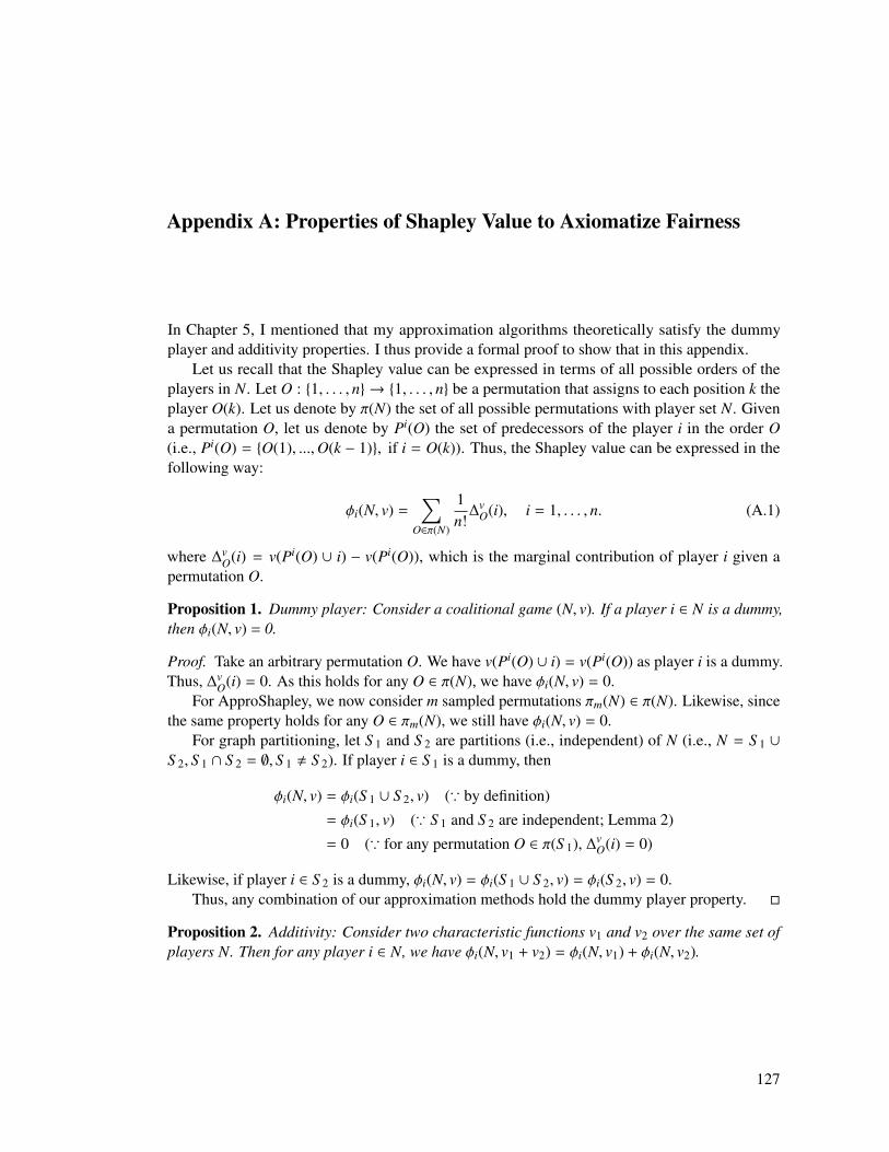
Appendix A: Properties of Shapley Value to Axiomatize Fairness

In Chapter 5, I mentioned that my approximation algorithms theoretically satisfy the dummyplayer and additivity properties. I thus provide a formal proof to show that in this appendix.

Let us recall that the Shapley value can be expressed in terms of all possible orders of theplayers in N. Let O : {1, . . . , n} → {1, . . . , n} be a permutation that assigns to each position k theplayer O(k). Let us denote by π(N) the set of all possible permutations with player set N. Givena permutation O, let us denote by Pi(O) the set of predecessors of the player i in the order O(i.e., Pi(O) = {O(1), ...,O(k − 1)}, if i = O(k)). Thus, the Shapley value can be expressed in thefollowing way:

φi(N, v) =∑

O∈π(N)

1n!

∆vO(i), i = 1, . . . , n. (A.1)

where ∆vO(i) = v(Pi(O) ∪ i) − v(Pi(O)), which is the marginal contribution of player i given a

permutation O.

Proposition 1. Dummy player: Consider a coalitional game (N, v). If a player i ∈ N is a dummy,then φi(N, v) = 0.

Proof. Take an arbitrary permutation O. We have v(Pi(O) ∪ i) = v(Pi(O)) as player i is a dummy.Thus, ∆v

O(i) = 0. As this holds for any O ∈ π(N), we have φi(N, v) = 0.For ApproShapley, we now consider m sampled permutations πm(N) ∈ π(N). Likewise, since

the same property holds for any O ∈ πm(N), we still have φi(N, v) = 0.For graph partitioning, let S 1 and S 2 are partitions (i.e., independent) of N (i.e., N = S 1 ∪

S 2, S 1 ∩ S 2 = ∅, S 1 , S 2). If player i ∈ S 1 is a dummy, then

φi(N, v) = φi(S 1 ∪ S 2, v) (∵ by definition)

= φi(S 1, v) (∵ S 1 and S 2 are independent; Lemma 2)

= 0 (∵ for any permutation O ∈ π(S 1), ∆vO(i) = 0)

Likewise, if player i ∈ S 2 is a dummy, φi(N, v) = φi(S 1 ∪ S 2, v) = φi(S 2, v) = 0.Thus, any combination of our approximation methods hold the dummy player property. �

Proposition 2. Additivity: Consider two characteristic functions v1 and v2 over the same set ofplayers N. Then for any player i ∈ N, we have φi(N, v1 + v2) = φi(N, v1) + φi(N, v2).

127

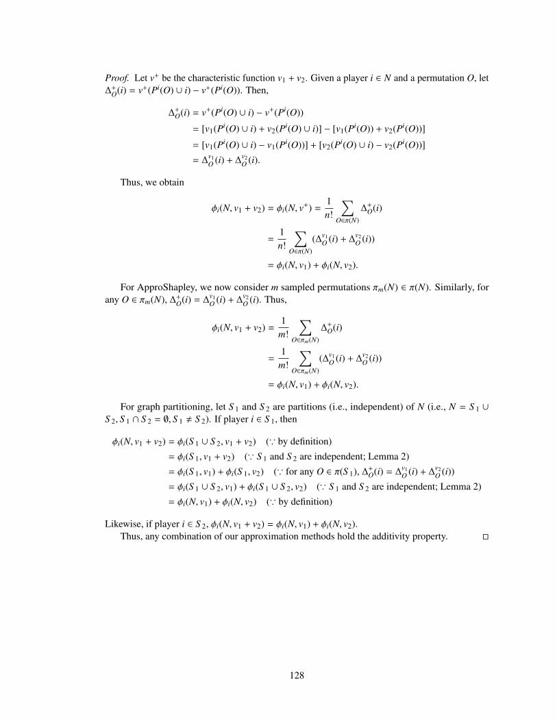
Proof. Let v+ be the characteristic function v1 + v2. Given a player i ∈ N and a permutation O, let∆+

O(i) = v+(Pi(O) ∪ i) − v+(Pi(O)). Then,

∆+O(i) = v+(Pi(O) ∪ i) − v+(Pi(O))

= [v1(Pi(O) ∪ i) + v2(Pi(O) ∪ i)] − [v1(Pi(O)) + v2(Pi(O))]

= [v1(Pi(O) ∪ i) − v1(Pi(O))] + [v2(Pi(O) ∪ i) − v2(Pi(O))]

= ∆v1O (i) + ∆

v2O (i).

Thus, we obtain

φi(N, v1 + v2) = φi(N, v+) =1n!

∑O∈π(N)

∆+O(i)

=1n!

∑O∈π(N)

(∆v1O (i) + ∆

v2O (i))

= φi(N, v1) + φi(N, v2).

For ApproShapley, we now consider m sampled permutations πm(N) ∈ π(N). Similarly, forany O ∈ πm(N), ∆+

O(i) = ∆v1O (i) + ∆

v2O (i). Thus,

φi(N, v1 + v2) =1

m!

∑O∈πm(N)

∆+O(i)

=1

m!

∑O∈πm(N)

(∆v1O (i) + ∆

v2O (i))

= φi(N, v1) + φi(N, v2).

For graph partitioning, let S 1 and S 2 are partitions (i.e., independent) of N (i.e., N = S 1 ∪

S 2, S 1 ∩ S 2 = ∅, S 1 , S 2). If player i ∈ S 1, then

φi(N, v1 + v2) = φi(S 1 ∪ S 2, v1 + v2) (∵ by definition)

= φi(S 1, v1 + v2) (∵ S 1 and S 2 are independent; Lemma 2)

= φi(S 1, v1) + φi(S 1, v2) (∵ for any O ∈ π(S 1), ∆+O(i) = ∆

v1O (i) + ∆

v2O (i))

= φi(S 1 ∪ S 2, v1) + φi(S 1 ∪ S 2, v2) (∵ S 1 and S 2 are independent; Lemma 2)

= φi(N, v1) + φi(N, v2) (∵ by definition)

Likewise, if player i ∈ S 2, φi(N, v1 + v2) = φi(N, v1) + φi(N, v2).Thus, any combination of our approximation methods hold the additivity property. �

128