Embed Size (px)
Citation preview

THE POSSIBILITY INDEX: AN INVESTMENT CRITERION
by
Toshio Suzuki
1998


CONTENTS
………………………………………………………………………………………PREFACE v
Section
………………………………………………………………………………I. INTRODUCTION 1……………………………………………………………II. THEORETICAL FRAMEWORK 3
…………………………………………………1 Some Theories on Investment Decision 3…………………………………………………………………………2 Possibility Index 5………………………………………………………………………3 Method of Analysis 6
……………………………………………III. MANUFACTURING INDUSTRIES IN INDIA 7……………………………………………………………………1 Cement Industry (3) 11
………………………………………………………………2 Electric Motor Industry (6) 12…………………………………………3 Ceramic Insulator (Low Tension) Industry (7) 12
………………………………………………………………………4 Lead Industry (8) 13…………………………………………IV. MANUFACTURING INDUSTRIES IN JAPAN 15
…………………………………V. FORMULATION OF THE INVESTMENT CRITERION 17……………………………………………1 The Way to Calculate the Possibility Index 17
……………………………………………………2 Calculation of the Desired Capacity 18……………………………………………………3 Calculation of the Possibility Index 18……………………………………………………4 Formulation of the Possibility Index 19
……………………………………………………………………………VI. CONCLUSION 23……………………………………………………………………………………APPENDICES 27
…………………………………………………………1 Source and Note of the Figures 27……………………………………………………………………………………2 Figures 32…………………………………………………………………………………3 TABLES 46
…………………………………………………………………SELECTED BIBLIOGRAPHY 53…………………………………………………………………1 Bibliography in English 53………………………………………………………………2 Bibliography in Japanese 55
iii


PREFACE
The topic of this paper is, as the title shows, to formulate an investment criterion. The re-search was focused on the Indian economy. But it is also useful for the economy of developedcountries.
v

I. INTRODUCTION
The topic of this paper is, as the title shows, to formulate an investment criterion. Authorhas devised an investment criterion and named it the Possibility Index (hereafter called the PI).This is the index which shows the possibility of growth of each sector. Here, the industry isclassified into each sector such as the Diesel Engine Industry, the Cement Industry, the Lead In-dustry, etc. The basic theory is to allocate the limited resources preferentially into the sector ofwhich the PI is relatively high or the possibility of growth is relatively high. The research is fo-cused on the Indian economy. But the PI is applicable to other economies also. The contents ofeach section are as follows.
In section II, the theoretical framework of PI is shown. Here, the exact way to calculate thePI is not specified. It is specified after examining the Indian and the Japanese economy. And, themethod of analysis of each sector of the Indian and the Japanese economy is shown.
In section III, the manufacturing industry in India is analyzed according to the method pre-scribed above.
In section IV, the manufacturing industry in Japan is analyzed. From the comparison be-tween these two countries, some serious problems in Indian economy were found.
In section V, the method to work out the PI is specified taking account of the results of sur-vey of both economies and the PI is worked out with regard to each sector.
In section VI, the final conclusions are drawn.In the appendix, all the figures and the tables are collected.
1

Quarterly1 J. J. Polak, "Balance of Payments Problems of Countries Reconstructing with the Help of Foreign Loans,"Journal of Economics International Investment and Domestic Welfare57 (February 1943): 208-40; and Norman S. Buchanan,(New York: Henry Colt, 1945), quoted in Subrata Ghatak, , 2nd ed. (London: AllenAn Introduction to Development Economics& Unwin, 1986), p. 85.
Alfred E. Kahn, "Investment Criteria in Development Programs," 65 (February 1951):2 Quarterly Journal of Economics38-61.
Hollis B. Chenery, "The Application of Investment Criteria," 67 (February 1953):3 Quarterly Journal of Economics76-96.
Quarterly4 Walter Galenson and Harvey Leibenstein, "Investment Criteria, Productivity, and Economic Development,"69 (August 1955): 343-70.Journal of Economics
Quarterly Journal of5Amartya K. Sen, "Some Notes on the Choice of Capital-Intensity in Development Planning,"
71 (November 1957): 561-84.Economics
Krishna K. Singh, (Delhi: Amar Prakashan, 1985), pp. 22-5.6 Investment Project in A Planned Economy
II. THEORETICAL FRAMEWORK
1 Some Theories on Investment Decision
In this section, some theories on investment decision in the development economics and themacroeconomics are briefly surveyed. Especially, they were surveyed with regard to the factorstaken into account and the determinant factors of in vestment decision.
J. J. Polak and N. S. Buchanan developed the Capital-Turnover Criterion. Polak concluded1
that resources must be allocated to the project where the rate of turnover is the highest.Alfred E. Kahn criticized Polak and Buchanan and developed the Social Marginal Productiv-
ity (SMP) Criterion. This criterion aims to maximize the national product by allocating the re-2
sources in the manner that makes the SMP of investment equal among all the projects.Hollis B. Chenery advanced this theory by taking account of the effect of investment on the
3balance of payment.Walter Galenson and Harvey Leibenstein criticized the SMP criterion and developed the re-
investment criterion. This criterion aims to make the investment into the project from which the4
largest amount of saving per unit of capital invested can be derived.Amartya K. Sen reviewed the capital-turnover criterion, the SMP criterion, and the reinvest-
ment criterion and put forward a fourth criterion which he called the time series criterion. This5
criterion aims to maximize the output within a certain period of time.Krishna K. Singh mentions, although this is not his original theory, the ratio of labor to in-
vestment criterion. This criterion aims to maximize the employment per unit of additional6
3
Ragnar Nurkse, (Oxford: Basil Blackwell Publisher Ltd.,1 Problems of Capital Formation in Under Developed Countries
1953; reprint ed., Delhi: Oxford University Press, 1973).
Paul N. Rosenstein-Rodan, "Problems of Industrialization of Eastern and South-Eastern Europe," 532 Economic Journal
(June- September 1943): 202-11; and Nurkse.
Albert O. Hirschman, "The Strategy of Economic Development," Precis of a lecture delivered at the Institute on ICA3
Accelerating Investment in Developing EconomiesDevelopment Programming; reprinted in A. N. Agarwala and S. P. Singh, ed.,(London: Oxford University Press, 1969), pp. 3-11; Charles P. Kindleberger, (NewThe Terms of Trade: A European Case Study
Oxford Economic Pa-York: Technology Press/Wiley, 1956), quoted in Ghatak, p. 98; and Paul Streeten, "Unbalanced Growth,"11 (June 1959): 167-90.pers
Tibor Scitovsky, "Two Concepts of External Economies," 62 (April 1954): 143-51.4 Journal of Political Economy
The5Hollis. B. Chenery, "The Interdependence of Investment Decisions: Essays in Honor of Bernard Francis Haley," in
, ed. Moses Abramovitz et al (Stanford: Stanford University Press, 1959), pp. 82-120.Allocation of Economic Resources
Larry E. Westphal, "Planning with Economies of Scale," in , ed.6 Economy Wide Models and Development PlanningCharles R. Blitzer, Peter B. Clark, and Lance Taylor (Oxford: Oxford University Press, 1975), pp. 257-306.
Structural Change and7 Hollis B. Chenery and Larry E. Westphal, "Economies of Scale and Investment over Time," in, A World Bank Research Publication, ed. Hollis B. Chenery (n.p.: Oxford University Press, 1979), pp. 217-Development Policy
67.
Economic Struc-8Larry E. Westphal and Jacques Cremer, "'The Interdependence of Investment Decisions' Revisited," in
, ed. Moshe Syrquin, Lance Taylor, and Larry E. Westphal (Orlando: Academic Press, Inc., 1984), pp.ture and Performance543-72.
John M. Keynes, (London: Macmillan & Co., Ltd., 1936; re-9 The General Theory of Employment, Interest and Moneyprint 4th ed., Tokyo: Maruzen Co., Ltd., 1973), p. 135.
4
1capital. Ragnar Nurkse supports this idea.Economists like Rosenstein-Rodan, Nurkse, etc. supported the balanced growth. On the2
other hand, economists like Albert O. Hirschman, Charles P. Kindleberger, Paul Streeten, etc.3supported the unbalanced growth.
The Cost-Benefit Analysis takes account of the cost-benefit ratio.In theories on external economies and economies of scale, Tibor Scitovsky distinguished two
types of external economies. One is discussed in the equilibrium theory and another is discussed4
in the theory of industrialization in underdeveloped countries.Chenery cited this Scitovsky's example of external economies and calculated the effect of it
5following this example.Larry E. Westphal showed some ways of calculating the effect of economies of scale using
the method of MIP (Mixed Integer Programing). Furthermore, Chenery and Westphal calculated6
the effect of economies of scale and timing of investment using a model with realistic assumptionabout the nature of horizontal and vertical interdependence. On the other hand, Westphal and7
Jacques Cremer extended the aforementioned Chenery's analysis on the interdependence of invest-ment decisions by analyzing the effect of interdependence on make-buy decisions under the as-
8sumption of existence of economies of scale.On the other hand, in the field of macroeconomics, John M. Keynes developed the theory of
9marginal efficiency of capital.In the theory of acceleration principle, the investment is dependent on the change in output
or GNP. But, Chenery introduced factors such as the flexible accelerator, the lag between the
Hollis B. Chenery, "Overcapacity and the Acceleration Principle," 20 (January 1952): 1-28.1 Econometrica
Dale W. Jorgenson, "Capital Theory and Investment Behavior," 53 (May 1963): 247-59.2 American Economic Review
James Tobin, "A General Equilibrium Approach to Monetary Theory," 1 (Feb-3 Journal of Money, Credit and Banking
ruary 1969): 15-29.
5
changes in demand and the new investment to meet new demand, and the optimum degree of1overcapacity.
D. W. Jorgenson developed a new theory called the neoclassical theory of investment. In2
the final result namely in the investment function, the investment depends on the desired capitalstock, and so it depends on the user cost of capital.
Tobin's q theory forms the main stream of recent investment theories. In this theory, the3
adjustment cost is taken into account. He mathematically got the following results.(1) q > 1 Net Investment > 0→
(2) q = 1 Net Investment = 0→
(3) q < 1 Net Investment < 0.→
2 Possibility Index
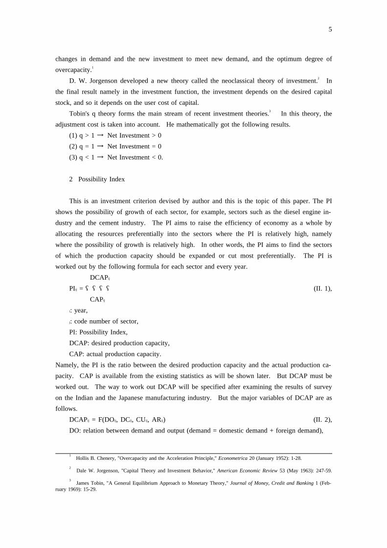
This is an investment criterion devised by author and this is the topic of this paper. The PIshows the possibility of growth of each sector, for example, sectors such as the diesel engine in-dustry and the cement industry. The PI aims to raise the efficiency of economy as a whole byallocating the resources preferentially into the sectors where the PI is relatively high, namelywhere the possibility of growth is relatively high. In other words, the PI aims to find the sectorsof which the production capacity should be expanded or cut most preferentially. The PI isworked out by the following formula for each sector and every year.
ijDCAPPI = (II. 1),ij ――――
ijCAP: year,i
: code number of sector,j
PI: Possibility Index,DCAP: desired production capacity,CAP: actual production capacity.
Namely, the PI is the ratio between the desired production capacity and the actual production ca-pacity. CAP is available from the existing statistics as will be shown later. But DCAP must beworked out. The way to work out DCAP will be specified after examining the results of surveyon the Indian and the Japanese manufacturing industry. But the major variables of DCAP are asfollows.
DCAP = F(DO , DC , CU , AR ) (II. 2),ij ij ij ij ij
DO: relation between demand and output (demand = domestic demand + foreign demand),
6
DC: relation between demand and production capacity,CU: capacity utilization,AR: availability of raw materials.The factors taken into account and the determinant factors of investment in the investment
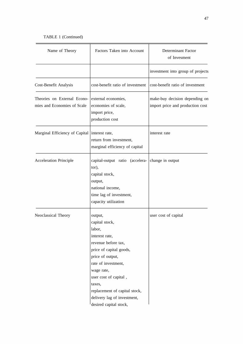
theories surveyed and the PI are shown in the TABLE 1. The differences between the PI andother investment theories will be examined in the conclusion.
3 Method of Analysis
The Indian and the Japanese manufacturing industries were surveyed with regard to the vari-ables of DCAP in order to analyze how these variables reflect the possibility of growth. Thesurvey was carried out, as we will see later, by drawing the data into the graphs and by compar-ing both of Indian and Japanese manufacturing industries. By analyzing all the data available andcomparing both Indian and Japanese manufacturing industries, some serious problems of Indianmanufacturing industries were found.
Statistical Ab-1 Government of India, Ministry of Planning, Department of Statistics, Central Statistical Organization,(New Delhi: Central Statistical Organization, Relevant Issues), (hereafter cited as GOI, ).stract Abstract
III. MANUFACTURING INDUSTRIES IN INDIA
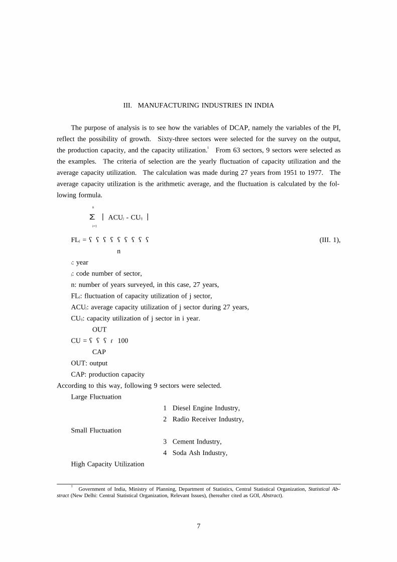
The purpose of analysis is to see how the variables of DCAP, namely the variables of the PI,reflect the possibility of growth. Sixty-three sectors were selected for the survey on the output,the production capacity, and the capacity utilization. From 63 sectors, 9 sectors were selected as1
the examples. The criteria of selection are the yearly fluctuation of capacity utilization and theaverage capacity utilization. The calculation was made during 27 years from 1951 to 1977. Theaverage capacity utilization is the arithmetic average, and the fluctuation is calculated by the fol-lowing formula.
n
∑ | |ACU - CUj ij
i=1
FL = (III. 1),j ―――――――――
n: yeari
: code number of sector,j
n: number of years surveyed, in this case, 27 years,FL : fluctuation of capacity utilization of j sector,j
ACU : average capacity utilization of j sector during 27 years,j
CU : capacity utilization of j sector in i year.ij
OUTCU = 100―――・
CAPOUT: outputCAP: production capacity
According to this way, following 9 sectors were selected.Large Fluctuation
1 Diesel Engine Industry,2 Radio Receiver Industry,
Small Fluctuation3 Cement Industry,4 Soda Ash Industry,
High Capacity Utilization
7

Raghunath K. Koti, , Gokhale Institute Mimeograph Series No. 91 Utilization of Industrial Capacity in India, 1967-68
(Poona: Gokhale Institute of Politics and Economics, n.d.), pp. 91-9.
8
5 Power Transformer Industry,6 Electric Motor Industry,
Low Capacity Utilization7 Ceramic Insulator Industry (low tension),8 Lead Industry,
Others9 Soap Industry.
The reason for selecting the Soap Industry is that the shape of graph was interesting to author.The production capacity is calculated according to the number of shift of operation. If the
shift number is 1, the production capacity is the output produced in 8 hours operation. If theshift number is 3, the production capacity is the output produced in 24 hours operation. The shift
1number of Cement Industry and Soda Ash Industry is 3 and that of other 7 sectors is 1.In this paper, the results of only the Cement Industry, the Electric Motor Industry, the Ce-
ramic Insulator Industry, and the Lead Industry are shown due to the restriction on pages. Theresults are drawn into graphs. For example, the graphs of the Cement Industry are shown in theFig. 1-5 (from Fig. 1 to Fig. 5). The sources and notes of data are shown in the section 1 of theAppendices.
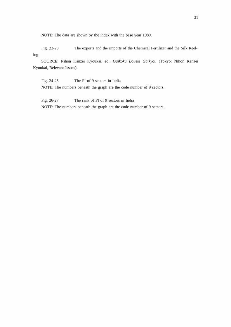
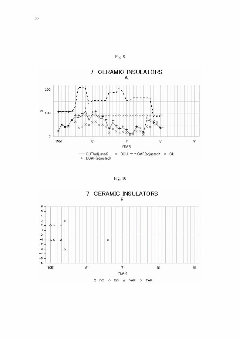
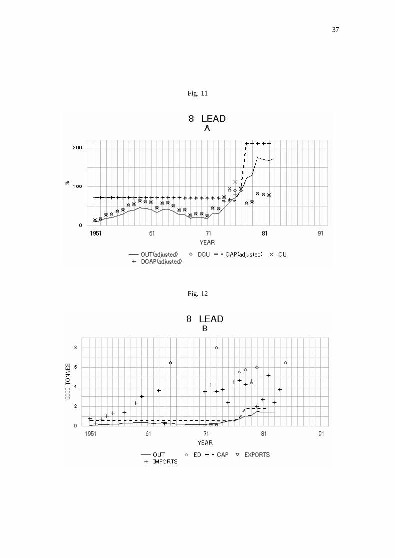
In the graph A, the output (OUT), the production capacity (CAP), the capacity utilization(CU), the desired capacity (DCAP), and the desired capacity utilization (DCU) are shown. Theunit of Y axis is percent (%). Therefore, CU and DCU can be read directly from the value of Yaxis. But, OUT, CAP, and DCAP are adjusted to the scale of Y axis. So the value of themcannot be read from the Y axis. The unit of them is shown in the note. In case of the CementIndustry, the unit of OUT, CAP, and DCAP is "tonnes." The original data are OUT and CAPonly. CU was calculated by author. DCAP and DCU, which will be mentioned in the section V,were also calculated by author.
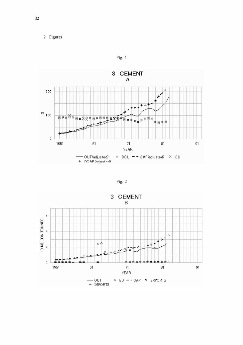
In the graph B, the output (OUT), the production capacity (CAP), the exports and imports(EXPORTS and IMPORTS), and the estimated demand (ED) are shown in real terms. The unitof each item is common, so each line can be compared directly.
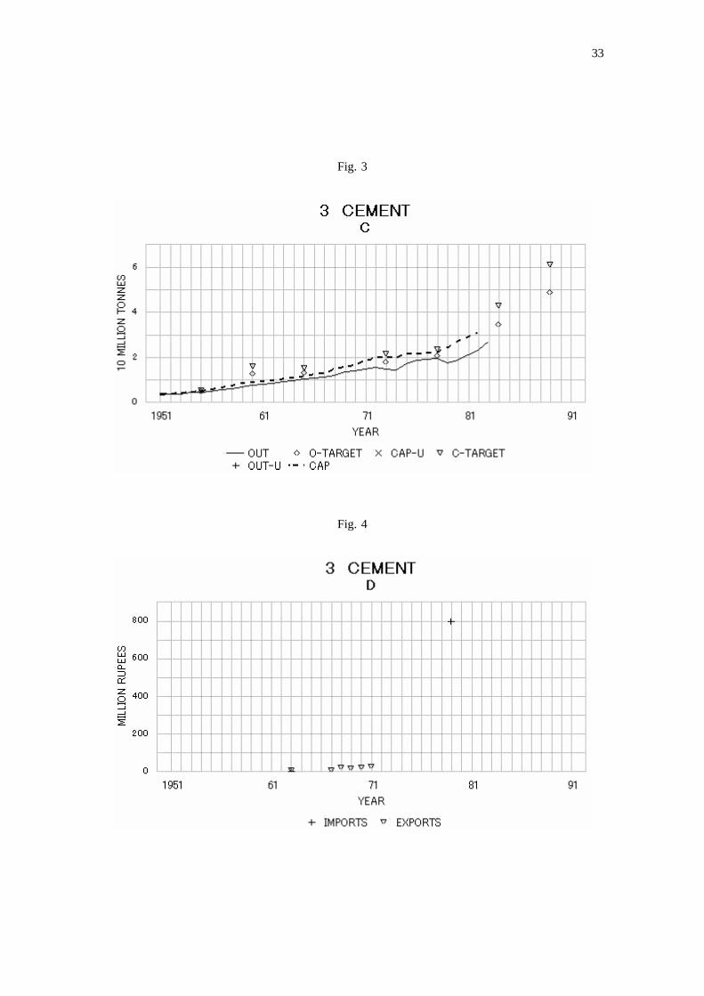
In the graph C, the output (OUT), the production capacity (CAP), the output in the unorgan-ized sector (OUT-U), the production capacity in the unorganized sector (CAP-U), the target ofoutput (O-TARGET), and the target of production capacity (C- TARGET) are shown. The unitis common among all items.
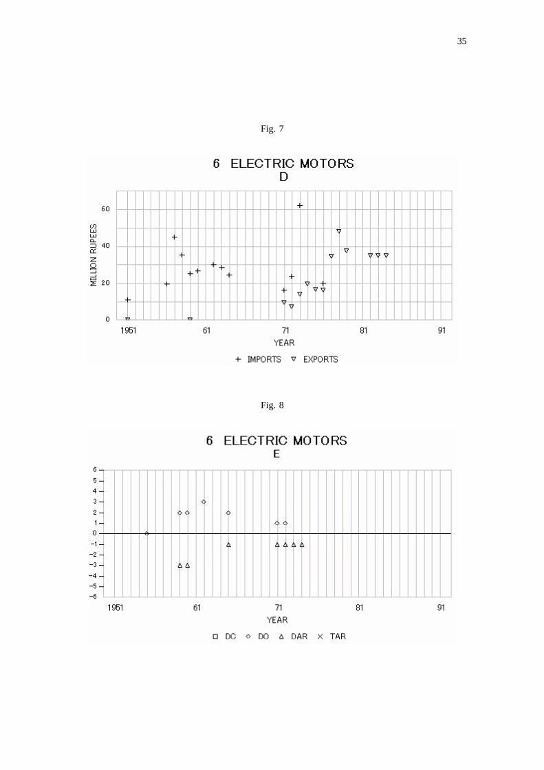
In the graph D, the exports (EXPORTS) and imports (IMPORTS) in money term are shown.This is also to see the situation of demand and supply. The exports and imports in real term areshown in the graph B. But the unit of them is not necessarily appropriate. For example, the unitof real term of the Electric Motor Industry is "horsepower." But there are some types of electricmotors. Namely, they are different in the horsepower and structure. So, the figures in terms ofmoney is also useful. And the data of each term are not available sufficiently, so two types of

Annual Survey of1 Government of India, Ministry of Planning, Department of Statistics, Central Statistical Organization,(Calcutta: Central Statistical Organization, Relevant Issues) (hereafter cited as GOI, ASI).Industries: Census Sector
9
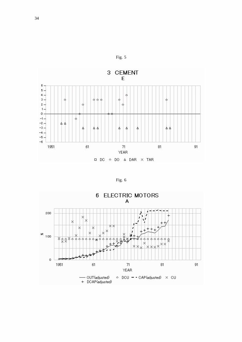
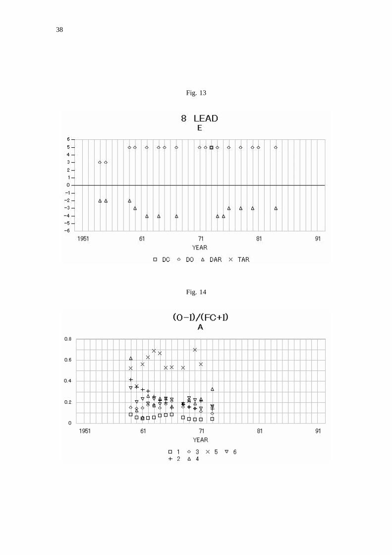
data can compliment with each other.In the graph E, the relation between the demand and the output (DO), the relation between
the demand and the production capacity (DC), the availability of raw materials within the country(DAR, Domestic Availability of Raw Materials), and the availability of raw materials includingthe imports (TAR, Total Availability of Raw Materials) are shown. The meaning of each item isas follows.
The relation between the demand and the output (DO) is divided into 11 classes.5: The demand exceeds the output to the maximum extent,4: Intermediate situation between 5 and 3,3: The supply is very inadequate,2: The shortage of supply is clearly reported,1: The shortage of supply is suggested,0: The demand and the supply are equal,
-1: The excess production is suggested,-2: The excess production is clearly reported,-3: The production is very excessive,-4: Intermediate situation between -3 and -5,-5: The production is excessive to the maximum extent.The relation between the demand and the production capacity (DC) is also divided into 11
classes.The domestic availability of raw materials (DAR) is divided into 6 classes.0: The raw materials are available sufficiently,
-1: The shortage is suggested,-2: The shortage is clearly reported,-3: The raw materials are very inadequate,-4: Intermediate situation between -3 and -5,-5: The raw materials are inadequate to the maximum extent.The availability of raw material including the imports (TAR) is also divided into 6 classes.The above four items are determined subjectively, not determined according to the objective
data. For example, if there is a report that the demand and the output is equal, DO is 0. And ifthere is a report that the output is very inadequate as compared with the demand, DO is 3. Here,the availability of raw material includes the availability of electric power, transport facility, etc.
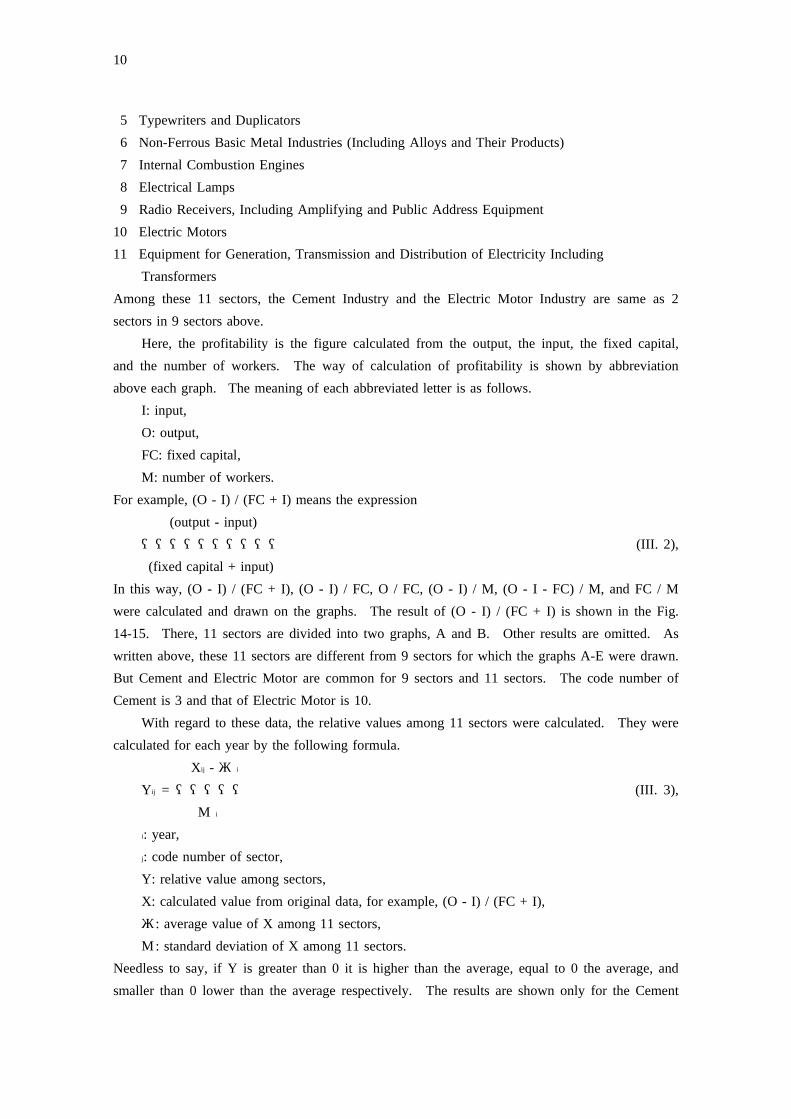
1The profitability was analyzed with regard to following 11 sectors.1 Flour Mills2 Soaps and Glycerine3 Cement (Hydraulic)4 Insulators
10
5 Typewriters and Duplicators6 Non-Ferrous Basic Metal Industries (Including Alloys and Their Products)7 Internal Combustion Engines8 Electrical Lamps9 Radio Receivers, Including Amplifying and Public Address Equipment
10 Electric Motors11 Equipment for Generation, Transmission and Distribution of Electricity Including
TransformersAmong these 11 sectors, the Cement Industry and the Electric Motor Industry are same as 2sectors in 9 sectors above.
Here, the profitability is the figure calculated from the output, the input, the fixed capital,and the number of workers. The way of calculation of profitability is shown by abbreviationabove each graph. The meaning of each abbreviated letter is as follows.
I: input,O: output,FC: fixed capital,M: number of workers.
For example, (O - I) / (FC + I) means the expression(output - input)
(III. 2),――――――――――
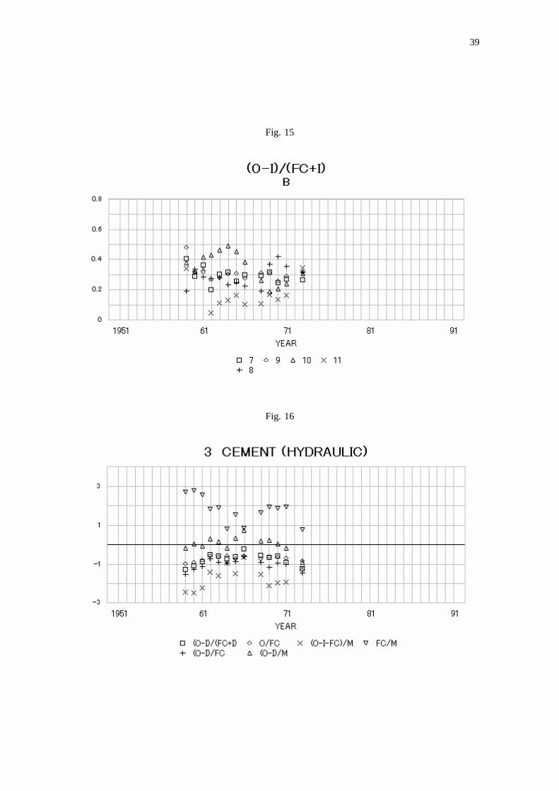
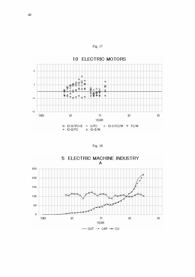
(fixed capital + input)In this way, (O - I) / (FC + I), (O - I) / FC, O / FC, (O - I) / M, (O - I - FC) / M, and FC / Mwere calculated and drawn on the graphs. The result of (O - I) / (FC + I) is shown in the Fig.14-15. There, 11 sectors are divided into two graphs, A and B. Other results are omitted. Aswritten above, these 11 sectors are different from 9 sectors for which the graphs A-E were drawn.But Cement and Electric Motor are common for 9 sectors and 11 sectors. The code number ofCement is 3 and that of Electric Motor is 10.
With regard to these data, the relative values among 11 sectors were calculated. They werecalculated for each year by the following formula.
ij iX - μY = (III. 3),ij ―――――
iσ
: year,i
: code number of sector,j
Y: relative value among sectors,X: calculated value from original data, for example, (O - I) / (FC + I),
: average value of X among 11 sectors,μ
: standard deviation of X among 11 sectors.σ
Needless to say, if Y is greater than 0 it is higher than the average, equal to 0 the average, andsmaller than 0 lower than the average respectively. The results are shown only for the Cement
The number in the parenthesis is the number of 9 sectors selected.1
Kothari & Sons, (Madras: Kothari & Sons, n.d.), p. 4 (Ce-2 Kothari's Economic and Industrial Guide of India, 1978-79
ment) (hereafter cited as K&S, ).Economic & Industrial Guide
For example, K&S, , p. 2-3 (Cement).3 Economic & Industrial Guide, 1973-1974
K&S, , p. 2 (Cement); and K&S, , p. 1 (Ce-4 Economic & Industrial Guide, 1973-74 Economic & Industrial Guide, 1976
ment).
K&S, , p. 4 (Cement).5 Economic & Industrial Guide, 1976
Kazuo Osugi ed., (Tokyo: Institute of Developing Economies, 1968), pp. 306-7.6 Indo: Keizai to Toushikankyou
_
11
Industry and the Electric Motor Industry in the Fig. 16-17.
11 Cement Industry (3)
As written above, the code number is 3 both among 9 sectors and 11 sectors. This sectorwas selected as an example of the small fluctuation of capacity utilization. The fluctuation of ca-pacity utilization is the smallest among 63 sectors. The average capacity utilization is 86.4%.But, as mentioned earlier, the production capacity of the Cement Industry and the Soda Ash In-dustry was calculated on the 3 shift basis. So, the 86.4% is close to the upper limit of capacityutilization. The graph A to E are shown in the Fig. 1-5. In case of the Cement Industry and theElectric Motor Industry, as mentioned above, the data of profitability are available. The profita-bility was analyzed about 11 sectors including the Cement Industry and the Electric Motor Indus-try. The profitability, (O - I) / (FC + I), of 11 sectors selected are shown in the Fig. 14-15. Therelative value was worked out by the formula (III. 3) and the results of the Cement Industry areshown in the Fig. 16.
It can be seen in the Fig. 1 or the TABLE 2 that the output has been growing steadily andthe production capacity has been expanded very smoothly following the output, and so the capaci-ty utilization has been stabilized very well. This forms a strong contrast to the Diesel Engine In-dustry and the Radio Receiver Industry although they were omitted. The situation of the CementIndustry looks very well. But, some serious problems were found in the survey.
The price and the distribution of cement has been under control for mostly all the period sur-→ → → →veyed. The relation that price control low price small profit inadequate investment2
shortage of cement was often reported. And the power cut, the voltage fluctuation, the inade-3
quate and irregular coal supply, the shortage of wagons for the transport of raw materials as well4as cement, and the labor troubles were the principal causes of the low capacity utilization.
5Sometimes the black market, where the price was three times the official price, emerged.The control of price and distribution was removed in order to stimulate the expansion of in-
dustry in January 1966. So, the price rose and, stimulated by this, the producers ventured on theexpansion of undertakings one after another. But, thereafter, the control was imposed again and6

Kothari & Sons, , (Madras: Kothari & Sons,1 Kothari's Economic Guide and Investors' Handbook of India, 1969-1970n.d.), p. 111 (hereafter cited as K&S, ).Economic Guide & Investors' Handbook
12
1the price was fixed.These situation can be observed in the graphs. In the Fig. 2, the estimated demand some-
times exceeds the output. In the Fig. 5, the demand-output relation (DO) often shows the supplyshortage. The domestic availability of raw materials (DAR) are often -3, meaning that the rawmaterials were often very inadequate.
On the other hand, the profitability is seen in the Fig. 14 where the code number of Cementis 3. The profitability did not fluctuate largely. The relative value of profitability among 11 sec-tors are seen in the Fig. 16. There, the fixed capital per labor (FC/M) is high but the labor pro-ductivity ((O - I) / M, (O - I - FC) / M) is low because the profitability of capital ((O - I) / (FC +I), (O - I) / FC, O / FC) is low.
Thus, the administered price and distribution are the serious problems in the Cement Indus-try.
2 Electric Motor Industry (6)
As written above, the code number is 6 among 9 sectors and 10 among 11 sectors. Thissector was selected because of its high capacity utilization. The average capacity utilization is106.1%, 3rd among 63 sectors and the fluctuation of capacity utilization is 7th.
In the Fig. 6-8, in the years the supply was inadequate, the capacity utilization was high andthe imports was much greater than the exports.
On the other hand, in the Fig. 15 where the code number of Electric Motor is 10, the profita-bility is high in the period 1959-66 while they are not so far from the average in the period1968-71. In the Fig. 17, the profitability of capital [(O - I) / (FC + I), (O - I) / FC, O / FC] isrelatively high in the period 1959-1966 as compared to the period 1968-1971. In the former pe-riod, larger shortage of supply was reported as compared with latter period (Fig. 8). The fixedcapital per worker (FC / M) is relatively low but the profitability of capital is high and the pro-ductivity of labor [(O - I) / M, (O - I - FC) / M] is mostly average or higher.
3 Ceramic Insulator (Low Tension) Industry (7)
This sector was selected as an example of the sectors of low capacity utilization. The aver-age capacity utilization was 36.5%, the lowest among 63 sectors and the fluctuation of capacityutilization was 35th.
In the Fig. 9 and the TABLE 2, the highest capacity utilization was 70.4% recorded in 1955and the lowest one was 7.7% recorded in 1972.
In the Fig. 10, from 1951 to 1955, inadequate supply of insulators and low availability ofraw materials were reported. But in the later period, the capacity utilization declined. The liter-
Guide-1 Government of India, Ministry of Industry, Department of Industrial Development, Indian Investment Centre,(New Delhi: Indian Investment Centre, 1973), p. 202 (hereafter cited as GOI, ).lines for Industries, 1973-74 Guidelines
Kothari & Sons, (Madras: Kothari & Sons, n.d.), p. 16 (Mining & Chemicals) (here-2 Investors' Encyclopaedia, 1955-56
after cited as K&S, ).Encyclopaedia
Koti, summarized from p. 29 and 45.3
13
ature concerned are not abound, so the cause is not known exactly. But it seems that the short-age of demand made the capacity utilization decline. The production capacity was not cut despitethe low capacity utilization. The reason seems to be that this industry was protected as a
1small-scale industry.
4 Lead Industry (8)
Also this sector was selected as an example of low capacity utilization. The average capaci-ty utilization is 49.2%, 59th among 63 sectors and the fluctuation of capacity utilization is 27th.
In the Fig. 11, the production capacity had not shown a large change until around 1976.The capacity utilization had stayed at low level for mostly all the period surveyed. From 1947 to1950, for which the data is not drawn into the graph, the capacity utilization had been between3.2% and 10.5%. Therefore, for 27 years ranging from 1947 to 1973, the capacity utilization2
was between 3.2% in 1947 and 64.9% in 1959.In the Fig. 12, the estimated demand shows the much higher value than the output, and in
many years the amount of import is several times or more than ten times the domestic production.In the Fig. 13, the shortage of raw materials and the lead are often reported. The extent of
shortage is, for the raw materials from 2 to 5, and for the supply of lead from 3 to 5 respectively.This means that the shortages are extremely serious for both the raw materials and the supply oflead. Thus, the capacity utilization was very low due to the inadequate supply of lead ore andthe supply of lead was inadequate. And so the lead has been imported by the amount severaltimes or more than ten times the domestic production.
We have seen that the capacity utilization was low due to the lack of demand in the CeramicInsulator Industry and due to the shortage of raw materials in the Lead Industry respectively. Asrepresented by these examples, in India, the major causes of low capacity utilization are two.One is the lack of demand and the other is the shortage of raw materials. Koti had conducted asurvey on 517 items. According to him, in the sectors of low capacity utilization, 42% of them isdue to the lack of demand, 21% to the shortage of raw materials, 4% to both causes, 17% to thelack of demand, the shortage of raw materials, the shortage of power, the labor trouble, and the
3lack of fund. Namely, 82% is related to the lack of demand or the shortage of raw materials.

Tsushousangyou Daijin Kanbou Chousa Toukeibu, ed. (Tokyo: Okurashou Insatsukyoku,1 Koukougyou Shisu Souran_ _ _
Souran KoukougyouRelevant Issues) (hereafter cited as MITI (Ministry of International Trade and Industry), ); and ----------,(Tokyo: Okurashou Insatsukyoku, 1981), pp. 64-74, and pp. 164-7 (hereafter cited as MITI, ).Shisu Nenpou, 1981 Nenpou
_
Okurashou, , Houjin Kigyou Toukei Nenpou Tokushu, (Tokyo: Okurashou Insatsukyoku,2 Zaisei Kin'yu Toukei Geppou
_ _ _ _
Zaisei Geppou Houjin Kigyou Toukei Nenpou,Relevant Issues) (hereafter cited as Okurashou, ); Okurashou Rizaikyoku Keizaika,_ _
(Tokyo: Okurashou Insatsukyoku, 1960), Relevant Pages (hereafter cited as Okurashou, ).1960 Kigyou Toukei_ _
IV. MANUFACTURING INDUSTRIES IN JAPAN
Regarding Japan also, same type of analysis was carried out as far as possible. Thirty sec-tors were selected for the survey of the output, the production capacity, and the capacity utiliza-tion. They were selected considering the continuity of data. Regarding the profitability, the1
2data are available for 12 sectors.In case of Japan, the output and the capacity utilization are shown by the index. And the
production capacity was calculated from above two variables by author. So the output and theproduction capacity cannot be compared directly on the graph like the Indian manufacturing in-dustries. And the capacity utilization of different sectors cannot be compared directly. But, aswe will see it, relative trend of progress can be seen from the graphs. Also the output and thecapacity utilization are available for the above 12 sectors of which the data of profitability areavailable.
Regarding the above 12 sectors, analyzed data on the profitability are, for example, as fol-lows.
Current ProfitPR = ,―――――――
Total CapitalPR: Profit Rate (current profit rate of total capital),Current Profit: sales amount + non-operating income - cost of sales - selling cost -general administrative cost - non-operating expenses,Total Capital: current assets + fixed assets + deferred assets.
Relative value of each data was calculated according to the expression (III. 3).Like the case of India, some sectors were selected for the further survey. But the capacity
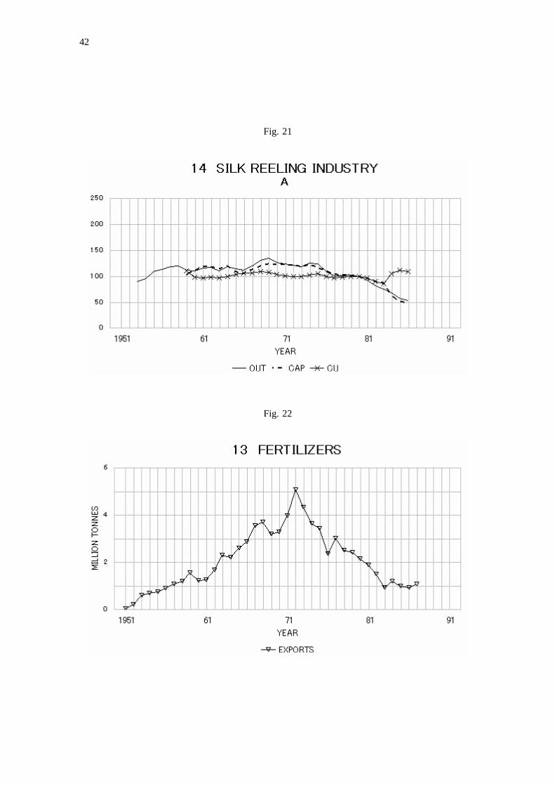
utilization is shown by the index and the fluctuation of capacity utilization is not so differentamong sectors. So the criterion of selection is different from that of India. Here, with regard tothe adjustment of production capacity, only the Electric Machine Industry, the Precision MachineIndustry, the Chemical Fertilizer Industry, and the Silk Reeling Industry are examined (Fig.18-21). Former two sectors are the examples of increasing rate of growth, and latter two sectorsare the examples of decreasing output. In case of the Electric Machine Industry and the Precision
15
Nihon Keizai Shinbunsha, ed., (Tokyo: Nihon Keizai Shinbunsha, 1987), p. 31.1 Zeminaru Nihon Keizai Nyumon
_ _
Hisao Kanamori, (Tokyo: Chuoukeizaisha, 1982), p. 11.2 Kouza Nihon Keizai - Jou: Keizai Shakai no Shikumi
16
Machine Industry, the output has been increasing with progressively increasing rate of growth.The production capacity has been expanded according to the increase in the output.
On the other hand, in case of the Chemical Fertilizer Industry and the Silk Reeling Industry,the output has been decreasing and the production capacity has been cut according to the decreasein the output. In case of the Chemical Fertilizer Industry, major causes of the decrease in outputwere two oil shocks. Also the decrease in the demand, the overcompetition, and the loss of in-ternational competitive power had made this industry a structural slump ridden industry. In the1
Fig. 22, the export of chemical fertilizer had been increasing until 1972 and thereafter began todecrease. It is observed that the production capacity has been cut according to the decrease in theexports (Fig. 20).
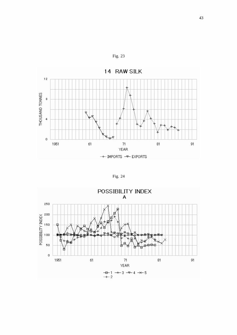
In case of the Silk Reeling Industry, the output had been gradually increasing until 1969 andthereafter turned to the decreasing trend. The silk had been the most important goods for exportuntil 1920's. But thereafter the exports decreased drastically due to the depression and the devel-opment of synthetic fiber in the USA. Since 1966, Japan has been importing the silk. We can2
see that the maximum point of production is very close to the point where the export of raw silkended and the import began (Fig. 23). Thus the production of the Silk Reeling Industry has de-creased due to the decrease in demand and so the production capacity has been adjusted accordingto the situation.
Regarding the profitability, the positive relation between the growth rate of output and thecurrent profit rate of total capital was observed although their graphs are omitted here.
V. FORMULATION OF THE INVESTMENT CRITERION
1 The Way to Calculate the Possibility Index
As mentioned in section II, the Possibility Index (PI), is the ratio between the desired capaci-ty and the actual capacity. It is written again. It is calculated by the following formula.
DCAPPI = 100 (V. 1),―――― ・
CAPDCAP: desired capacity,CAP: actual capacity.CAP is available from the existing statistics, so the surveys on the Indian and the Japanese
manufacturing industries have been conducted in order to find the way to calculate DCAP. Ex-amining the data and information available, the possible and best way to calculate the PI seems tobe as follows. DCAP is worked out on the basis of Optimal Capacity Utilization (OCU). TheOptimal Capacity Utilization is the rate at which the profit rate is the maximum or the productionis the most profitable. So, it is different from a company to a company, or from a sector to asector. Here, OCU is set at 90.0%. But, even if it is set at 80.0%, it does not affect the resultsconsiderably as will be shown later. The method of calculation is different according to thesituation of capacity utilization, demand and supply, availability of raw materials, etc. The meth-od is specified as follows according to the situation.
A. CU 90.0%≧
B. CU 90.0% due to the lack of demand<
C. CU 90.0% due to the shortage of raw materials, but the supply is inadequate<
CU: capacity utilizationIn case of A, the Electric Motor Industry can be cited as an example. In that industry, there
are many years in which the capacity utilization was above 90.0% and the demand was excessiveas compared with the production capacity. So the production capacity must be expanded in orderto lower the capacity utilization to 90.0%. So DCAP is worked out by the following formula,
OUTDCAP = (V. 2),――――
0.900OUT: actual output.
Namely, DCAP is the production capacity which yields OCU.In case of B, the Ceramic Insulator Industry can be cited as an example. In this case, the
capacity utilization was low due to the lack of demand so the production capacity should be cut
17
18
according to the demand. So in this case also, DCAP is worked out by the formula (V. 2).In case of C, the Lead Industry can be cited. In case of the Lead Industry, the demand was
much larger than the production capacity but the capacity utilization was very low due to theshortage of raw materials. So it is fruitless to expand the production capacity because the com-pany cannot increase the out put with the increased capacity due to the shortage of raw materials.And also, it is fruitless to cut the production capacity to raise the capacity utilization becausethere exists a sufficient demand as compared with the production capacity. Therefore, it is desir-able to maintain the present production capacity and to supply sufficient raw materialsimmediately. Therefore, DCAP is worked out by the following formula,
DCAP = CAP (V. 3).If we got DCAP by the above way, we can calculate the desired capacity utilization (DCU).
DCU is worked out by the following formula.OUT
DCU = (V. 4).――――
DCAPDCU is the rate at which the sector operates with actual output OUT and DCAP. So OCU is90.0% but DCU can be below 90.0% as we will see it later.
DCAP, DCU, and the PI were worked out with regard to the Indian 9 sectors selected ac-cording to the way above.
2 Calculation of the Desired Capacity
For example, the situation of the Cement Industry are shown in the Fig. 1-5. In 1951, thecapacity utilization was 89.8% and there is no report that the supply was inadequate. But, takingaccount of the situation around this period, it seems that the supply was inadequate (Fig. 5). SoDCAP was worked out by the formula (V. 3). From 1952 to 1955, in 1960, and from 1963 to1965, the capacity utilization was at or above 90.0%, so DCAP was worked out by the formula(V. 2). DCAP of remaining years, except for 1958, 1959, 1967, and 1968, were worked out bythe formula (V. 3), because the capacity utilization was below 90.0% but the supply seemed to beinadequate. In 1958, 1959, 1967, and 1968, the capacity utilization was below 90.0% and thesupply was adequate or excessive (Fig. 5). So DCAP was worked out by the formula (V. 2).
The results are shown in the Fig. 1. With regard to DCU, it is sometimes equal to anddifferent from actual capacity utilization. This depends on the situation of market as writtenabove. DCAP of other 9 sectors were worked out by the similar way.
3 Calculation of the Possibility Index
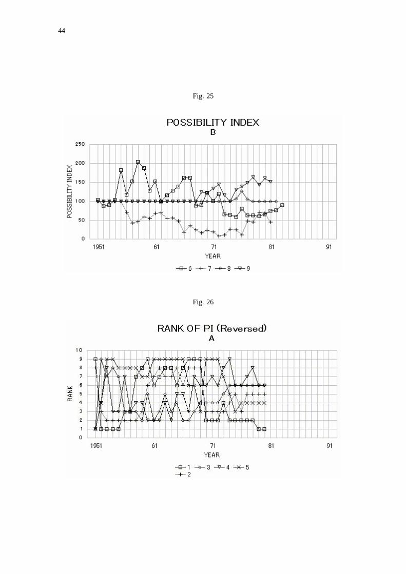
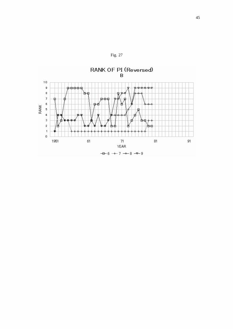
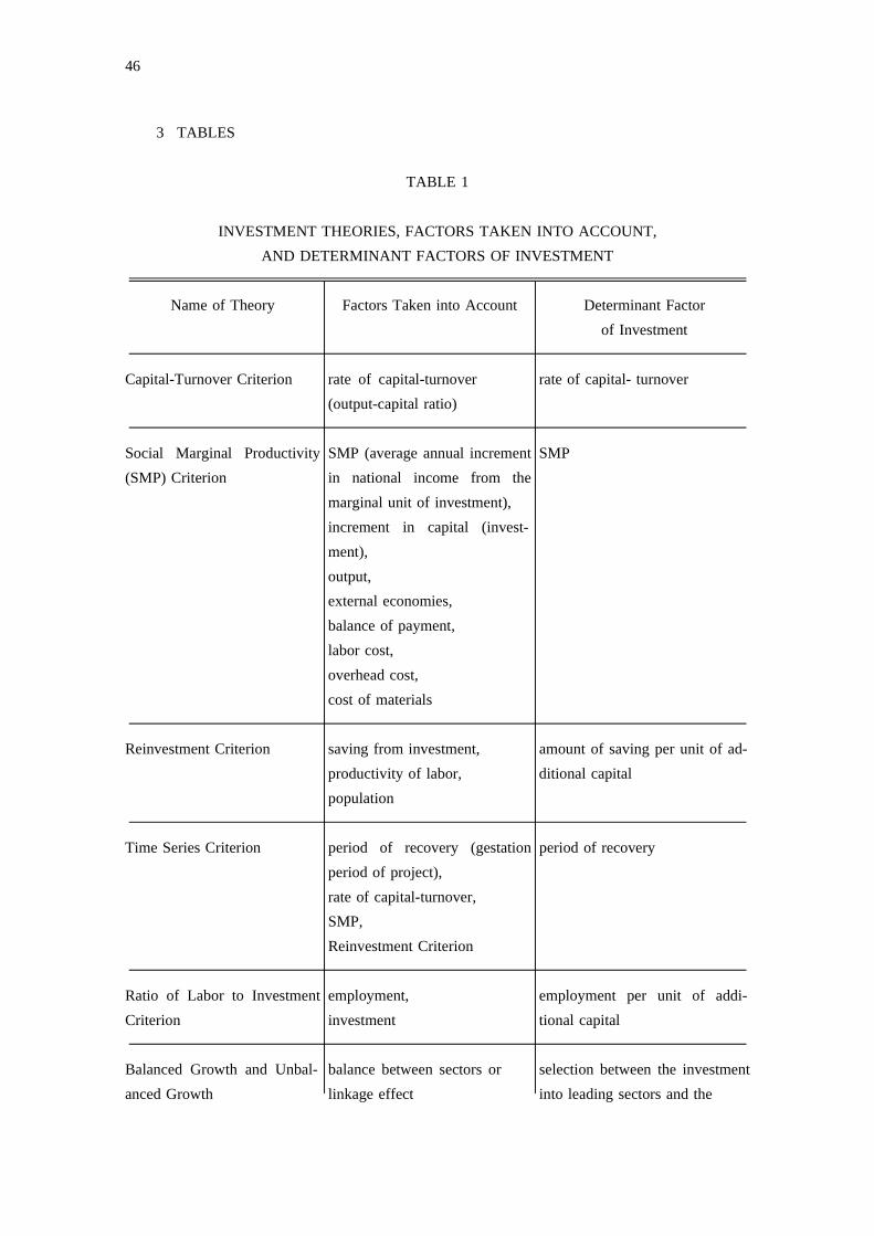
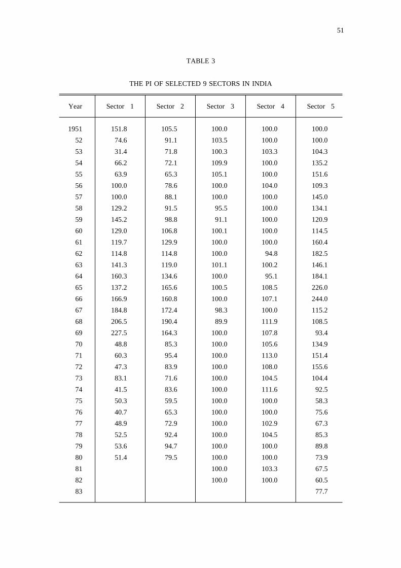
We have worked out DCAP, so now we can work out the PI by the formula (V. 1). The re-sults are shown in the Fig. 24-25 and the TABLE 3. Nine sectors are divided into two graphs.The rank of PI is shown in the Fig. 26-27. There, the rank is reversed so that we can optically
19
compare the graphs of the PI and the rank. Namely, if the PI is highest the rank is 9, and if thePI is lowest the rank is 1.
For example, in case of the Cement Industry (code number of sector is 3), the PI is near orequal to 100.0. But the rank ranges from 9th to 1st. For example, the PI is 100.0 in 1951 and1956. But the rank is 1st in 1951 and 3rd in 1956. This is because the rank is the relative valueamong 9 sectors.
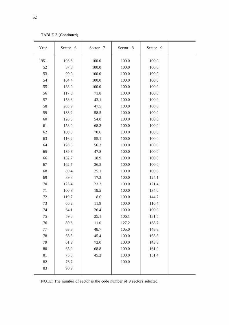
Thus we can see the PI and the rank of it. Observing all the 9 sectors, we can see followingsituation. In the first decade namely from 1951 to 1960, the PI of the Electric Motor Industry (6)shows high value, and the Ceramic Insulator Industry (7) shows low value. Their ranks are at thetop or the bottom in some years respectively. From 1961 to 1970, the Diesel Engine Industry (1)and the Power Transformer Industry (5) show high value, and the Ceramic Insulator Industry (7)shows low value. The ranks of Diesel Engine Industry (1) and the Power Transformer Industry(5) are at the top in some years, and the rank of the Ceramic Insulator Industry (7) is always atthe bottom. From 1971 to 1980, the Power Transformer Industry (5) and the Soap Industry (9)show high value, the Diesel Engine Industry (1) and the Electric Motor Industry (6) declined tolow level, and the Ceramic Insulator Industry (7) turned to the rising trend after showing the ex-tremely low level. The Power Transformer Industry (5) and the Soap Industry (9) are at the toprank in some years respectively. The Diesel Engine Industry (1) declined to the bottom rank, andthe Electric Motor Industry (6) declined to the 2nd rank. The Ceramic Insulator Industry (7) roseup to the 3rd rank after staying at the bottom for 23 years. As for the Lead Industry (8), al-though the capacity utilization was very low in many years, the PI is 100.0 in most years due tothe reasons mentioned above.
4 Formulation of the Possibility Index
So far, we have examined the data available and have worked out the PI from them. So, wemust specify the necessary and technically possible data for the PI and the way to work out the PIwith them.
The calculation of the PI is carried out according to the formula (V. 1). The basis of calcu-lation is OCU (optimal capacity utilization). OCU is the rate at which the profit rate is the maxi-mum. In the calculation above, OCU was set at 90.0%. But even if it was set at 80.0% or atother values, the results does not affect seriously at least with regard to the sectors near the toprank or the bottom rank. We have seen it above. So far, we have adopted 90.0% as OCU forall the sectors concerned. But we should specify OCU for each sector. For example, in the ironand steel industry, the blast furnace cannot be turned off so easily, so the operation must be con-tinued throughout the day. Therefore, OCU must be necessarily close to 300.0% on the one shiftbasis. But, in many industries, OCU can be far below 300.0%. In case of cement industry, thecapacity utilization was shown on three sift basis but in other industries the capacity utilizationwas shown on one sift basis. Also this problem must be solved. OCU must be worked out foreach sector taking account of the features of each sector. The way to specify OCU cannot be
20
specified here. Author must leave this problem for the later research.Here, OCU was defined as the most profitable capacity utilization. But, the capacity utiliza-
tion at which the profit rate is zero may be more appropriate. Let us call this the minimum re-quired capacity utilization (MRCU). The profit is positive above MRCU, the profit is zero atMRCU , and the profit is negative below MRCU. MRCU may be more easily worked out thanOCU.
From the above analysis, we can specify the statistics necessary for the calculation of DCAPand OCU or MRCU.
1 Output and Production Capacity,2 Estimated Demand (including the information on demand and supply situation of the
products in the market),3 Availability of Raw Materials (including the electric power, transport facility, labor force,
etc.),4 Profitability,5 Exports and Imports.The specification of these statistics must follow the criteria below.1. The classification of sector must be common among the statistics. For example, the
classifications of sector for the profitability and for the output and production capacity are notcommon. This is the serious obstacle to the analysis. Secondly, the unit of output and produc-tion capacity must be coordinated. For example, in the Electric Motor Industry, the unit is horse-power. But there are so many types of electric motors. Some motors have small horsepowerand some have big horsepower, and the structure of electric motor is not same. We can solvethis problem by setting a standard product. For example, we can set the electric motor of onehorsepower and of popular structure as a standard product. Other types of electric motors can beconverted into this standard product in terms of the cost of production. Namely, if the cost ofelectric motor of other type is three times the standard electric motor, one unit of this motor isconverted into three units of the standard motor. Thus, every type of electric motor can be con-verted into the standard electric motor.
2. The classification of sector must be modified. Namely, if some types of electric motorscan be manufactured by the same production facility, they should be classified as in the same sec-tor. But, if they cannot, they should be classified as in the different sectors. But, for example,even if the electric motor and the power transformers can be manufactured by the same produc-tion facility, they cannot be classified as in the same sector because the purposes are different.
So far, we have worked out the PI from the existing data. Now, we can specify the way towork out the PI with the data specified above. The capacity utilization adopted as the base ofcalculation is OCU or MRCU. Here, the capacity utilization is shown on one shift basis and thecapacity utilization adopted as the basis is OCU set at 90.0%. The way to work out DCAP isshown according to each case bellow. Basically, the ways of calculation are composed of threecases.
A. 90.0% CU 300.0%, if CU is 300%, the production capacity is fully utilized.≦ ≧
21
B. CU 90.0%, due to the lack of demand.<
C. CU 90.0%, but the supply is inadequate due to the shortage of raw materials or other<
reasons.CU: capacity utilizationIn case of A, basically, DCAP is worked out by the following formula.
OUTDCAP = (V. 2),―――
0.900OUT: output.
This is because 90.0% CU and so production capacity should be increased according to the≦
output. But, the case A is further divided into four cases according to the relation between thesupply of and the demand for product, and to the situation of availability of raw materials.
In case A-1, CU = 300%, the supply is inadequate, and further raw materials are availablesufficiently.
In case A-2, CU = 300%, the supply is inadequate, and further raw materials are notavailable.
In case A-3, CU = 300%, the supply is adequate.In case A-4, 90% CU 300%.≦ >
In case A-1, the production capacity is fully utilized but the supply is inadequate. In thiscase, actual demand is greater than the output. So, DCAP is worked out by the formula
EDDCAP = (V. 5),―――
0.900ED: estimated demandIn case A-2, further raw materials are not available, so it is impossible to increase the output.
So, DCAP should be worked out by the formula (V. 2).In case A-3, the supply is adequate, so the output needs not be increased. So, DCAP is
worked out by the formula (V. 2).The case A-4 is divided into two cases. In case A-4-1, the supply is adequate. In this case,
DCAP is worked out by the formula (V. 2) because the output needs not be increased. In caseA-4-2, the supply is inadequate and the raw materials are inadequate. If the raw materials areavailable sufficiently, the output will increase. In this case, the output needs to be increased inorder to meet the demand. But it is impossible to increase the output because the raw materialsare inadequate. So, DCAP is worked out by the formula (V. 2), not by the formula (V. 5).Thus in case A as a whole, only in case A-1, DCAP is worked out by the formula (V. 5). Inother cases, DCAP is worked out by the formula (V. 2).
In case B, DCAP is worked out by the formula (V. 2). Because CU 90.0% due to the<
lack of demand.In case C, this case is divided into two cases. In case C-1,

22
ED(V. 6).――― ≧ 0.900
CAPED: estimated demand
This means CAP is optimal or less as compared with ED. So if the raw materials are suppliedsufficiently, CU will be 90.0%. But it is fruitless to increase the production capacity because≧
of shortage of raw materials. So DCAP is worked out by the formulaDCAP = CAP (V. 3).
In case C-2,ED
(V. 7).――― < 0.900
CAPThis means CAP is excessive as compared with ED. So DCAP is worked out by the formula (V.5).
As a whole, the formula (V. 2) is used in case, A-2, A-3, A-4, and B. The formula (V. 3) isused in case C-1. The formula (V. 5) is used in case A-1 and C-2.
Thus, we can work out DCAP more precisely with the modified statistical system specifiedabove. And, the PI is worked out by the formula
DCAPPI = 100 (V. 1).―――― ・
CAP
VI. CONCLUSION
As mentioned earlier, the purpose of research is to formulate a practical investment criterion,not an abstract one. In this regard, it seems that the PI is superior to other theories in the recog-nition of reality. For each theory surveyed, the factors taken into account and the determinantfactor of investment are listed in the TABLE 1.
As a whole, the theories surveyed take account of the profitability of firms or projects con-cerned but do not take account of the present market situation. But, as we have seen in the anal-ysis of the Indian manufacturing industries, the supply of products and the demand for it do notnecessarily coincide, and the raw materials are not always available sufficiently. On the otherhand, the PI can incorporate these factors into its system. This difference is quite crucial whenwe need the practical investment criterion.
However, the linkage effect, which was taken into account in the theories of the balancedgrowth and the unbalanced growth and in the theory on external economies and economies ofscale, cannot be incorporated. This is the weak point of the PI. But, it is very difficult to meas-ure the linkage effect covering the economy as a whole because the Input-Output Table is neces-sary to calculate the linkage effect over the economy as a whole. In this case, if the industry isclassified into the sector like the data for capacity utilization, the number of sectors will amountto several hundreds. Furthermore, the I-O table is necessary for every year. But, at the presentsituation of statistical system, it is impossible to work out such an I-O table every year. Further-more, in case of India, the data are available from the organized sector only, not available fromthe unorganized sector. So, it is mostly impossible to work out the linkage effect accurately. Sothe best way was to give up calculating the linkage effect and to work out the PI which does nottake account of the linkage effect.
As the conclusion, we must evaluate the reliability of the PI as an investment criterion. ThePI, like other investment criteria, cannot be the perfect criterion. But what we can expect fromthe PI is the more efficient investment, not the perfect investment. If, for example, 500 sectorsare selected for the analysis and the PI of each sector is calculated, we cannot say that the PI isreliable with regard to two sectors of which the ranks are 250th and 251st. But, with regard totwo sectors of which the ranks are 1st and 250th, the PI can be highly reliable. We can find thesectors at or near the top rank and the sectors at or near the bottom rank respectively. Namely,we can find the sectors of which the production capacity should be increased or cut most prefer-entially. The immediate adjustment of the production capacity according to the situation is cru-cial for the Indian economy to grow faster, as we have seen in the comparable analysis on the In-dian and the Japanese economy.
However, prompt adjustment of production capacity according to the PI is not always
23
Touyou Keizai, , First Series in 1990 (Tokyo: Touyou Keizai, December 1989), pp. 179-81.1 Kaisha Shikihou
Touyou Keizai, pp. 350-2.2
Touyou Keizai, pp. 612-4.3
Nihon Keizai Shinbunsha, p. 29.4
24
appropriate. For example, the military forces, educational system, health and welfare organiza-tions, some social infrastructures such as railway or road, etc. should not be adjusted according tothe possibility of growth. But, most manufacturing industries operating in the market economyshould be. Cutting the production capacity according to the PI may cause unemployment. Butfor this concern, we should examine the case of the Textile Industry. As we have seen in thesurvey of the Japanese manufacturing industries, the production in the Textile Industry has beenstagnated. Especially, the production in the Silk Reeling Industry has been decreasing. Manytextile companies cut the production capacity and reduced the production. But some textile com-panies had diversified their management and their current profit hit the highest record in their his-tory. For example in case of Teijin, one of the biggest textile companies in Japan, its composi-tion of sales is Tetron (synthetic fiber) 52, Nylon 9, Other Textile 3, Chemical Synthetic Products23, Medicine 12, Technical Plan and Others 1 in September 1989. The company has achieved thehighest record of current profit in its history in March 1989 (the end of fiscal year) and is goingto break the record at the end of next fiscal year. Other companies such as Toray Industries and
1Asahi Chemical Industries are also in the similar situation.The examples of diversification can be seen in other industries also. In case of the Iron and
Steel Industry, it is said that "The iron is the state." Thus, this industry is one of the most im-portant industries in Japan. But its status in the world is declining due to the competition fromabroad. So some companies are also diversifying the management into the field such as the in-formation, communication, electronic products, real property, etc. In the Shipbuilding Industry2
3also, some companies are diversifying the management.It is said the life cycle of one industry is 30 years. One industry is born, grows, gets ma-
tured, and gets old. This period is said to be 30 years. Therefore, most industry must always4
adjust its management according to the changes in the situation.Finally, we should examine the future perspective of the possible contribution of the PI.
Author has specified the necessary statistics for the PI. These statistics needs radical modifica-tion of the existing statistical system. But if they become available, we can work out the morereliable PI. If some countries in the world adopt the new statistic system for PI, the internationalcomparison will be possible. The PI will be useful not only for the developing countries but alsofor the industrialized countries because there is no country where there is no control of the econo-my by the government. On of the most remarkable international specifications of statistics is theI-O table. The Institute of Developing Economies in Japan sent the experts to the ASEAN coun-tries to instruct the local staffs. So today, the international I-O table, which works as an I-O table
Institute of Developing Economies (I.D.E), , I.D.E. Statis-1 International Input-Output Table for ASEAN Countries, 1975
tical Series, no. 39 (Tokyo: Institute of Developing Economies, 1982).
25
including multiple countries, is available. In the table, Indonesia, Peninsular Malaysia, Philip-1
pines, Singapore, Thailand, Japan, Korea, and U.S.A. are linked in one I-O table. If the statisticsystem for PI is introduced into each country like the international I-O table, it will become avery important data to observe the situation of world economy.

APPENDICES
1 Source and Note of the Figures
Fig. 1-13 (From the Fig. 1 to the Fig. 13)
The graphs from A to E of 4 sectors selected
In the graph A, the relation between the data and the line is as follows.OUT (output, adjusted to the scale of CU)DCAP (desired production capacity, adjusted to the scale of CU)++++++
DCU (desired capacity utilization)◇◇◇◇◇◇
----------------- CAP (production capacity, adjusted to the scale of CU)CU (capacity utilization)××××××
In the graph B, the relation between the data and the line is as follows.OUT (output)
IMPORTS (imports)++++++
ED (estimated demand)◇◇◇◇◇◇
------------------ CAP (production capacity)EXPORTS (exports)▽▽▽▽▽▽
In the graph C, the relation between the data and the line is as follows.OUT (output)OUT-U (output in the unorganized sector)++++++
O-TARGET (output target)◇◇◇◇◇◇
------------------ CAP (production capacity)CAP-U (production capacity in the unorganized sector)××××××
C-TARGET (capacity target)▽▽▽▽▽▽
In the graph D, the relation between the data and the line is as follows.IMPORTS (imports)++++++
EXPORTS (exports)▽▽▽▽▽▽
In the graph E, the relation between the data and the line is as follows.DC (demand-capacity ratio, relation between the demand and the production□□□□□□
27
28
capacity)DO (demand-output ratio, relation between the demand and the output)◇◇◇◇◇◇
DAR (domestic availability of raw materials, availability of raw materials in the△△△△△△
domestic market)TAR (total availability of raw materials, total availability of raw materials includ-××××××
ing the imports)
The unit and source of data of the Fig. 1-13 are as follows.
Fig. 1 3 CEMENT ASOURCE
OUT and CAP: GOI, , Relevant Issues. Other data were calculated by author.AbstractNOTE: Unit of OUT and CAP is tonnes.
Fig. 2 3 CEMENT BSOURCE
OUT and CAP: Same as the Fig. 1. EXPORTS: Government of India, Directorate of Public Re-Handbook of Industriallations and Publications, Directorate General of Technical Development,
(New Delhi: Directorate General of Technical Development, 1975), Relevant Issues (hereaf-Datater cited as GOI, ); K&S, , p. 67; andHandbook Economic Guide and Investors' Handbook, 1961Kothari Enterprises, (Madras: Kothari Enterprises,Kothari's Industrial Directory of India, 1986n.d.), p. 7 (Cement) (hereafter cited as Kothari, ). IMPORTS: GOI, , p.Directory Handbook, 1966141; K&S, , p. 67; and Kothari, ,Economic Guide and Investors' Handbook, 1961 Directory, 1986p. 3 and 7 (Cement). ED: GOI, , p. 142; GOI, , Relevant Issues;Guidelines, 1978/79 HandbookGovernment of India, Planning Commission, (New Delhi: PlanningSixth Five Year Plan, 1980/85
Sixth Plan Economic & IndustrialCommission, n.d.), p. 48 (hereafter cited as GOI, ); K&S,, p. 3 and 5 (Cement); K&S, , RelevantGuide, 1973/74 Economic Guide and Investors' Handbook
Issues; K&S, , Relevant Issues; and Kothari, , p. 2 (Cement).Encyclopaedia Directory, 1986
Fig. 3 3 CEMENT CSOURCE
Hand-OUT and CAP: Same as the Fig. 1. O-TARGET: Confederation of Engineering Industry,, 19th ed. (Delhi: Confederation of Engineering Industry, December 1986),book of Statistics, 1986
Handbook Guidelines, 1986/87 Handbook,p. 116 (hereafter cited as CEI, ); GOI, , p. 113; GOI,1973 Economic Guide and Investors' Handbook, 1969/70 Di-, p. 255; K&S, , p. 110; and Kothari,rectory, 1986 Handbook, 1986 Guidelines,, p. 3 (Cement). C-TARGET: CEI, , p. 116; GOI,1986/87 K&S, Economic & Industrial Guide, 1973/74 Economic, p. 113; , p. 1 (Cement); K&S,
, p. 110; K&S, , p. 2 (Cement); andGuide and Investors' Handbook, 1969/70 Encyclopaedia, 1954Kothari, , p. 3.Directory, 1986
29
Fig. 4 3 CEMENT DSOURCE
EXPORTS: GOI, , Relevant Issues. IMPORTS: GOI, , p. 141; andHandbook Handbook, 1966GOI, , p. 75.Sixth Plan
Fig. 5 3 CEMENT ESOURCE
Guidelines, 1973/74 Handbook, 1966 Economic & Indus-DO: GOI, , p. 203; GOI, , p. 141; K&S,, Relevant Issues; K&S, , Relevant Issues;trial Guide Economic Guide and Investors' Handbook
Encyclopaedia Directory, 1986 Guide-K&S, , Relevant Issues; and Kothari, , p. 8. DAR: GOI,lines, 1986 Economic & Industrial Guide Economic Guide, p. 113; K&S, , Relevant Issues; K&S,
, Relevant Issues; K&S, , Relevant Issues; and Kothari,and Investors' Handbook Encyclopaedia, p. 6.Directory, 1986
Fig. 6 6 ELECTRIC MOTORS ASOURCE
OUT and CAP: Same as the Fig. 1. Other data were calculated by author.NOTE: Unit of OUT and CAP is horsepower.
Fig. 7 6 ELECTRIC MOTORS DSOURCE
Guidelines Handbook, 1975 Economic &EXPORTS: GOI, , Relevant Issues; GOI, , p. 87; K&S,Industrial Guide, 1978/79 Economic Guide and Investors' Handbook,, p. 28 (Engineering); K&S,
, p. 117; and K&S, , p. 542. IMPORTS: GOI, ,1961 Encyclopaedia, 1956/57 Guidelines, 1979/80p. 14; GOI, , p. 87; K&S, , RelevantHandbook, 1975 Economic Guide and Investors' HandbookIssues; and K&S, , p. 541.Encyclopaedia, 1956/57
Fig. 8 6 ELECTRIC MOTORS ESOURCE
Guidelines Handbook, 1966 K&S, Economic Guide andDO: GOI, , Relevant Issues; GOI, , p. 41;, Relevant Issues; and K&S, , Relevant Issues. DAR: GOI,Investors' Handbook Encyclopaedia
Guidelines Handbook Economic Guide and Inves-, Relevant Issues; GOI, , Relevant Issues; K&S,, p. 116; and K&S, , pp. 170-1.tors' Handbook, 1961 Encyclopaedia, 1960
Fig. 9 7 CERAMIC INSULATORS ASOURCE
OUT and CAP: Same as the Fig. 1. Other data were calculated by author.NOTE: Unit of OUT and CAP is numbers from 1951 to 1956 and thereafter tonnes.
Fig. 10 7 CERAMIC INSULATORS E
30
SOURCEDO: Government of India, Ministry of Commerce and Industry, Development Commissioner(Small Scale Industries), [The title in English is notTeiatsu You Zetsuen Touki, (Toubu Chihou)known], Hon'yaku Shiryou no. 27, Indo Chushoukougyou Shir izu, no. 27, trans. Osaka Ajia
_ _ _
Chushoukigyou Kaihatsu Senta (n. p. : Osaka Ajia Chushoukigyou Kaihatsu Senta, 1965), Rele-_ _ _ _ _
vant Pages (hereafter cited as GOI, ); and K&S, , Relevant Issues.Zetsuen Touki EncyclopaediaDAR: GOI, , Relevant Pages; and K&S, , Relevant Issues.Zetsuen Touki Encyclopaedia
Fig. 11 8 LEAD ASOURCE
OUT and CAP: Same as the Fig. 1. Other data were calculated by author.NOTE: Unit of OUT and CAP is tonnes.
Fig. 12 8 LEAD BSOURCE
OUT and CAP: Same as the Fig. 1. EXPORTS: GOI, , p. 59. IMPORTS: GOI,Handbook, 1975Guidelines Handbook Economic & Industrial, Relevant Issues; GOI, , Relevant Issues; K&S,Guide, 1978/79 Economic Guide and Investors' Handbook,, p. 28 (Minerals & Metals); K&S,1961 Guidelines Handbook,, p. 245 (Mining & Chemicals). ED: GOI, , Relevant Issues; GOI,
, p. 149; GOI, , p. 49; and K&S, , Rele-1973 Sixth Plan Economic Guide and Investors' Handbookvant Issues.
Fig. 13 8 LEAD ESOURCE
Handbook, 1973 Guidelines Handbook,DC: GOI, , p. 149. DO: GOI, , Relevant Issues; GOI,1966 Economic & Industrial Guide Economic Guide and In-, p. 59; K&S, , Relevant Issues; K&S,
, Relevant Issues; and K&S, , Relevant Issues. DAR: GOI,vestors' Handbook Encyclopaedia, Relevant Issues; K&S, , Relevant Issues;Guidelines Economic Guide and Investors' Handbook
K&S, , Relevant Issues; and Koti, pp. 74-5.Encyclopaedia
Fig. 14-15 Profitability of 11 sectors selectedSOURCE: GOI, ASI, Relevant Issues.
Fig. 16-17 Relative value of profitability of the cement and the electric motorsamong 11 sectors
SOURCE: same as the Fig. 14-15.
Fig. 18-21 The out put, the production capacity, and the capacity utilization of 4sectors in Japan
SOURCE: MITI, , pp. 70-8; and ----------, , Relevant Issues.Nenpou, 1987 Souran
31
NOTE: The data are shown by the index with the base year 1980.
Fig. 22-23 The exports and the imports of the Chemical Fertilizer and the Silk Reel-ing
SOURCE: Nihon Kanzei Kyoukai, ed., (Tokyo: Nihon KanzeiGaikoku Boueki GaikyouKyoukai, Relevant Issues).
Fig. 24-25 The PI of 9 sectors in IndiaNOTE: The numbers beneath the graph are the code number of 9 sectors.
Fig. 26-27 The rank of PI of 9 sectors in IndiaNOTE: The numbers beneath the graph are the code number of 9 sectors.
32
2 Figures
Fig. 1
Fig. 2
33
Fig. 3
Fig. 4
34
Fig. 5
Fig. 6
35
Fig. 7
Fig. 8
36
Fig. 9
Fig. 10
37
Fig. 11
Fig. 12
38
Fig. 13
Fig. 14
39
Fig. 15
Fig. 16
40
Fig. 17
Fig. 18

41
Fig. 19
Fig. 20
42
Fig. 21
Fig. 22
43
Fig. 23
Fig. 24
44
Fig. 25
Fig. 26
45
Fig. 27
46
3 TABLES
TABLE 1
INVESTMENT THEORIES, FACTORS TAKEN INTO ACCOUNT,AND DETERMINANT FACTORS OF INVESTMENT
Name of Theory Factors Taken into Account Determinant Factorof Investment
Capital-Turnover Criterion rate of capital-turnover rate of capital- turnover(output-capital ratio)
Social Marginal Productivity SMP (average annual increment SMP(SMP) Criterion in national income from the
marginal unit of investment),increment in capital (invest-ment),output,external economies,balance of payment,labor cost,overhead cost,cost of materials
Reinvestment Criterion saving from investment, amount of saving per unit of ad-productivity of labor, ditional capitalpopulation
Time Series Criterion period of recovery (gestation period of recoveryperiod of project),rate of capital-turnover,SMP,Reinvestment Criterion
Ratio of Labor to Investment employment, employment per unit of addi-Criterion investment tional capital
Balanced Growth and Unbal- balance between sectors or selection between the investmentanced Growth linkage effect into leading sectors and the
47
TABLE 1 (Continued)
Name of Theory Factors Taken into Account Determinant Factorof Invesment
investment into group of projects
Cost-Benefit Analysis cost-benefit ratio of investment cost-benefit ratio of investment
Theories on External Econo- external economies, make-buy decision depending onmies and Economies of Scale economies of scale, import price and production cost
import price,production cost
Marginal Efficiency of Capital interest rate, interest ratereturn from investment,marginal efficiency of capital
Acceleration Principle capital-output ratio (accelera- change in outputtor),capital stock,output,national income,time lag of investment,capacity utilization
Neoclassical Theory output, user cost of capitalcapital stock,labor,interest rate,revenue before tax,price of capital goods,price of output,rate of investment,wage rate,user cost of capital ,taxes,replacement of capital stock,delivery lag of investment,desired capital stock,

48
TABLE 1 ( )Continued
Name of Theory Factors Taken into Account Determinant Factorof Invesment
net worth
Tobin's q Theory market value of firm, q (ratio between market value ofreplacement cost of capital, firm and replacement cost ofadjustment cost, capital)capital stock,labor,output,price of output,wage rate,capital cost
Possibility Index (PI) output, PI (ratio between the desired ca-production capacity, pacity and the actual capacity)capacity utilization,profitability,availability of raw materials,imports and exports,ratio between the demand andsupply in the market,estimated demand
SOURCE: Summarized from section II.
49
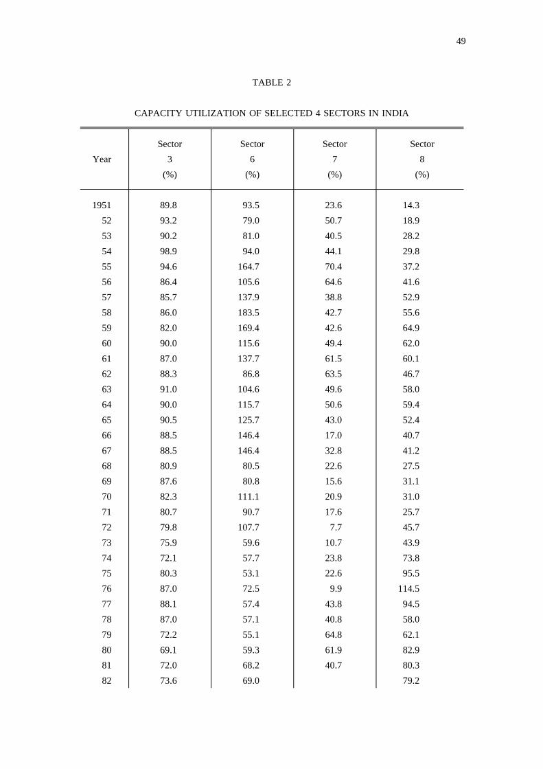
TABLE 2
CAPACITY UTILIZATION OF SELECTED 4 SECTORS IN INDIA
Sector Sector Sector SectorYear 3 6 7 8
(%) (%) (%) (%)
1951 89.8 93.5 23.6 14.352 93.2 79.0 50.7 18.953 90.2 81.0 40.5 28.254 98.9 94.0 44.1 29.855 94.6 164.7 70.4 37.256 86.4 105.6 64.6 41.657 85.7 137.9 38.8 52.958 86.0 183.5 42.7 55.659 82.0 169.4 42.6 64.960 90.0 115.6 49.4 62.061 87.0 137.7 61.5 60.162 88.3 86.8 63.5 46.763 91.0 104.6 49.6 58.064 90.0 115.7 50.6 59.465 90.5 125.7 43.0 52.466 88.5 146.4 17.0 40.767 88.5 146.4 32.8 41.268 80.9 80.5 22.6 27.569 87.6 80.8 15.6 31.170 82.3 111.1 20.9 31.071 80.7 90.7 17.6 25.772 79.8 107.7 7.7 45.773 75.9 59.6 10.7 43.974 72.1 57.7 23.8 73.875 80.3 53.1 22.6 95.576 87.0 72.5 9.9 114.577 88.1 57.4 43.8 94.578 87.0 57.1 40.8 58.079 72.2 55.1 64.8 62.180 69.1 59.3 61.9 82.981 72.0 68.2 40.7 80.382 73.6 69.0 79.2

50
TABLE 2 ( )Continued
Sector Sector Sector SectorYear 3 6 7 8
(%) (%) (%) (%)
1983 81.8
NOTE: The number of sector is the number of 9 sectors selected.
51
TABLE 3
THE PI OF SELECTED 9 SECTORS IN INDIA
Year Sector 1 Sector 2 Sector 3 Sector 4 Sector 5
1951 151.8 105.5 100.0 100.0 100.052 74.6 91.1 103.5 100.0 100.053 31.4 71.8 100.3 103.3 104.354 66.2 72.1 109.9 100.0 135.255 63.9 65.3 105.1 100.0 151.656 100.0 78.6 100.0 104.0 109.357 100.0 88.1 100.0 100.0 145.058 129.2 91.5 95.5 100.0 134.159 145.2 98.8 91.1 100.0 120.960 129.0 106.8 100.1 100.0 114.561 119.7 129.9 100.0 100.0 160.462 114.8 114.8 100.0 94.8 182.563 141.3 119.0 101.1 100.2 146.164 160.3 134.6 100.0 95.1 184.165 137.2 165.6 100.5 108.5 226.066 166.9 160.8 100.0 107.1 244.067 184.8 172.4 98.3 100.0 115.268 206.5 190.4 89.9 111.9 108.569 227.5 164.3 100.0 107.8 93.470 48.8 85.3 100.0 105.6 134.971 60.3 95.4 100.0 113.0 151.472 47.3 83.9 100.0 108.0 155.673 83.1 71.6 100.0 104.5 104.474 41.5 83.6 100.0 111.6 92.575 50.3 59.5 100.0 100.0 58.376 40.7 65.3 100.0 100.0 75.677 48.9 72.9 100.0 102.9 67.378 52.5 92.4 100.0 104.5 85.379 53.6 94.7 100.0 100.0 89.880 51.4 79.5 100.0 100.0 73.981 100.0 103.3 67.582 100.0 100.0 60.583 77.7
52
TABLE 3 (Continued)
Year Sector 6 Sector 7 Sector 8 Sector 9
1951 103.8 100.0 100.0 100.052 87.8 100.0 100.0 100.053 90.0 100.0 100.0 100.054 104.4 100.0 100.0 100.055 183.0 100.0 100.0 100.056 117.3 71.8 100.0 100.057 153.3 43.1 100.0 100.058 203.9 47.5 100.0 100.059 188.2 58.5 100.0 100.060 128.5 54.8 100.0 100.061 153.0 68.3 100.0 100.062 100.0 70.6 100.0 100.063 116.2 55.1 100.0 100.064 128.5 56.2 100.0 100.065 139.6 47.8 100.0 100.066 162.7 18.9 100.0 100.067 162.7 36.5 100.0 100.068 89.4 25.1 100.0 100.069 89.8 17.3 100.0 124.170 123.4 23.2 100.0 121.471 100.8 19.5 100.0 134.072 119.7 8.6 100.0 144.773 66.2 11.9 100.0 116.474 64.1 26.4 100.0 100.075 59.0 25.1 106.1 131.576 80.6 11.0 127.2 138.777 63.8 48.7 105.0 148.878 63.5 45.4 100.0 163.679 61.3 72.0 100.0 143.880 65.9 68.8 100.0 161.081 75.8 45.2 100.0 151.482 76.7 100.083 90.9
NOTE: The number of sector is the code number of 9 sectors selected.
53
SELECTED BIBLIOGRAPHY
1 Bibliography in English
Agarwala, A. N., and Singh S. P., ed. . Lon-Accelerating Investment in Developing Economiesdon: Oxford University Press, 1969.
Buchanan, Norman S. . New York: Henry Colt,International Investment and Domestic Welfare1945. Quoted in Subrata Ghatak, , 2nd ed., p .An Introduction to Development Economics85. London: Allen & Unwin, 1986.
Chenery, Hollis B. "Overcapacity and the Acceleration Principle." 20 (JanuaryEconometrica1952): 1-28.
----------. "The Application of Investment Criteria." 67 (Febru-Quarterly Journal of Economicsary 1953): 76-96.
The Allocation of Economic Re-----------. "The Interdependence of Investment Decisions." In, pp. 82-120. Edited by Mosessources: Essays in Honor of Bernard Francis Haley
Abramovitz et al. Stanford: Stanford University Press, 1959.Structur-----------, and Westphal, Larry E. "Economies of Scale and Investment over Time." In
, A World Bank Research Publication, pp. 217-67. Edit-al Change and Development Policyed by Hollis B. Chenery. n.p.: Oxford University Press, 1979.
Confederation of Engineering Industry. . 19th ed. Delhi: Confed-Handbook of Statistics, 1986eration of Engineering Industry, December 1986.
Galenson, Walter, and Leibenstein, Harvey. "Investment Criteria, Productivity, and EconomicDevelopment." 69 (August 1955): 343-70.Quarterly Journal of Economics
Ghatak, Subrata. . 2nd ed. London: Allen & Unwin,An Introduction to Development Economics1986.
Hirschman, Albert O. "The Strategy of Economic Development." Precis of a lecture deliveredat the Institute on ICA Development Programming; reprinted in Agarwala and S. P. Singh,pp. 3-11.
India, Government of, Directorate of Public Relations and Publications, Directorate General ofTechnical Development. . New Delhi: Directorate General ofHandbook of Industrial DataTechnical Development, Relevant Issues.
----------, Ministry of Industry, Department of Industrial Development, Indian Investment Centre.. New Delhi: Indian Investment Centre, Relevant Issues.Guidelines for Industries
Annual----------, Ministry of Planning, Department of Statistics, Central Statistical Organization.. Calcutta: Central Statistical Organization, RelevantSurvey of Industries: Census Sector
Issues.
54
----------, ----------, ----------. . New Delhi: Central Statistical Organization,Statistical AbstractRelevant Issues.
----------, Planning Commission. . New Delhi: Planning Commis-Sixth Five Year Plan, 1980/85sion, n.d.
International Input-Output Table for ASEAN Coun-Institute of Developing Economies (I.D.E).. I.D.E. Statistical Series, no. 39. Tokyo: Institute of Developing Economies,tries, 1975
1982.Jorgenson, Dale W. "Capital Theory and Investment Behavior," 53American Economic Review
(May 1963): 247-59.Quarterly Journal of Eco-Kahn, Alfred E. "Investment Criteria in Development Programs."
65 (February 1951): 38-61.nomicsKeynes, John M. . London: MacmillanThe General Theory of Employment, Interest and Money
& Co., Ltd., 1936; reprint 4th ed., Tokyo: Maruzen Co., Ltd., 1973.Kindleberger, Charles P. . New York: TechnologyThe Terms of Trade: A European Case Study
Press/Wiley, 1956. Quoted in Ghatak, p. 98.Kothari & Sons. . Madras: Kothari & Sons, Relevant Issues.Investors' Encyclopaedia----------. . Madras: Kothari & Sons, RelevantKothari's Economic and Industrial Guide of India
Issues.----------. . Madras: Kothari &Kothari's Economic Guide and Investors' Handbook of India
Sons, Relevant Issues.Kothari Enterprises. . Madras: Kothari Enterprises,Kothari's Industrial Directory of India, 1986
n.d.Koti, Raghunath K. . Gokhale InstituteUtilization of Industrial Capacity in India, 1967-68
Mimeograph Series, No. 9. Poona: Gokhale Institute of Politics and Economics, n.d.Nurkse, Ragnar. . Oxford: BasilProblems of Capital Formation in Underdeveloped Countries
Blackwell Publisher Ltd., 1953; reprint ed., Delhi: Oxford University Press, 1973.Polak, J. J. "Balance of Payment Problems of Countries Reconstructing with the Help of Foreign
Loans." 57 (February 1943): 208-40.Quarterly Journal of EconomicsRosenstein-Rodan, Paul N. "Problems of Industrialization in Eastern and South-Eastern Europe."
53 (June-September 1943): 202-11.Economic JournalScitovsky, Tibor. "Two Concepts of External Economies." 62Journal of Political Economy
(April 1954): 143-51.Sen, Amartya K. "Some Note on the Choice of Capital-Intensity in Development Planning."
71 (November 1957): 561-84.Quarterly Journal of EconomicsSingh, Krishna K. . Delhi: Amar Prakashan, 1985.Investment Project in A Planned EconomyStreeten, Paul. "Unbalanced Growth." 11 (June 1959): 167-90.Oxford Economic Papers
Journal of Money,Tobin, James. "A General Equilibrium Approach to Monetary Theory."1 (February 1969): 15-29.Credit and Banking
Economy Wide Models and Devel-Westphal, Larry E. "Planning with Economies of Scale," In, pp. 257-306. Edited by Charles R. Blitzer, Peter B. Clark, and Lanceopment Planning
55
Taylor. Oxford: Oxford University Press, 1975.----------, and Cremer, Jacques. "'The Interdependence of Investment Decisions' Revisited," In
, pp. 543-72. Edited by Moshe Syrquin, Lance Taylor,Economic Structure and Performanceand Larry E. Westphal. Orlando: Academic Press, Inc., 1984.
2 Bibliography in Japanese
India, Government of, Ministry of Commerce and Industry, Development Commissioner (SmallScale Industries). [The title in English is notTeiatsu You Zetsuen Touki, (Toubu Chihou)known.]. Hon'yaku Shiryou no. 27. Indo Chushoukougyou Shir izu, no. 27. Translated by
_ _
Osaka Ajia Chushoukigyou Kaihatsu Senta. n.p.: Osaka Ajia Chu-shoukigyou Kaihatsu_ _ _ _ _
Senta, 1965._
Kanamori, Hisao. . Tokyo: Chuoukeizaisha,Kouza Nihon Keizai - Ge: Keizai Shakai no Shikumi_
1982.----------. . Tokyo: Chuoukeizaisha, 1982.Kouza Nihon Keizai - Jou: Keizai Shakai no Shikumi
_
Nihon Kanzei Kyoukai, ed. . Tokyo: Nihon Kanzei Kyoukai, RelevantGaikoku Boueki GaikyouIssues.
Nihon Keizai Shinbunsha, ed. . Tokyo: Nihon KeizaiZeminaru Nihon Keizai Nyumon_ _
Shinbunsha, 1987.Okurashou. . Houjin Kigyou Toukei Nenpou Tokushu. Tokyo:Zaisei Kin'yu Toukei Geppou_ _ _
Okurashou Insatsukyoku, Relevant Issues._
----------, Rizaikyoku Keizaika. , 1960. Tokyo: OkurashouHoujin Kigyou Toukei Nenpou_
Insatsukyoku, 1960.Touyou Keizai. . First Series in 1990. Tokyo: Touyou Keizai, December 1989.Kaisha ShikihouTsushousangyou Daijin Kanbou Chousa Toukeibu, ed. . Tokyo:Koukougyou Shisu Nenpou_
Okurashou Insatsukyoku, Relevant Issues._
----------. . Tokyo: Okurashou Insatsukyoku, Relevant Issues.Koukougyou Shisu Souran_ _