The Political Economy of Exchange Rate

Regime Duration:

A Survival Analysis

by Ralph Setzer1

Abstract

This paper examines the role that political, institutional and economic factors played in

exchange rate regime duration in 49 developing countries within the time period 1974-2000.

Set in the framework of survival analysis, I characterize and model the times to exit for a

fixed exchange rate regime using a Cox model. The empirical analysis shows that exchange

rate regime choice is not a purely theoretical issue, but strongly depends on partisan and

institutional incentives such as the political colour of the government in power, the number of

veto players and the degree of central bank independence.

JEL classification: E61, F31, F33

Keywords: political economy, exchange rate regime, survival analysis, Cox model

I thank Ansgar Belke, Felix Hammermann, Hans Pitlik and Lars Wang for helpful comments

and Gian-Maria Milesi-Ferretti and Jakob de Haan for delivering valuable data. I also profited

very much from comments by participants at the IMAD and R.O.S.E.S. conference

"Institutions and Policies for the New Europe", in Portoroz (Slovenia), 16-19th June 2004.

1 University of Hohenheim, Department of Economics, Museumsflügel, 70599 Stuttgart, Germany, rasetzer@uni-hohenheim.de

2

1. Introduction

There is an extensive theoretical and empirical literature on the optimal exchange rate

arrangement for developing countries. Economists focused for most of the time on the

possible influence of optimal currency area (OCA) criteria such as trade openness or factor

mobility. These factors indeed have turned out to be crucial. However, structural variables of

the OCA approach cannot explain why among economies with similar economic structure,

large differences in exchange rate policy have been observed. More recent studies on the

determinants of exchange rate regime choice have therefore directed their attention to the

impact of domestic and institutional factors. Activated by a growing body of scholarship that

describes economic outcomes as influenced by government institutions, a number of

economists have claimed that electoral, partisan and institutional incentives have a significant

impact on exchange rate policy (see, e.g., Bernhard and Leblang 1999, Frieden, Ghezzi, and

Stein 2001). These authors argue that exchange rate policy is the outcome of a political

process with strong distributional and welfare implications. In this view, differences in

exchange rate policy can be explained by factors such as different parties having different

macroeconomic preferences, incumbents’ efforts to increase their reelection prospects, or by

interest groups that lobby for strong or weak currencies. The aim of this paper is to expand the

present literature on the political economy of exchange rate regimes in developing countries.

The central claim is that political and institutional factors have an important, predictable

impact on the duration of fixed exchange rate regimes. I use a survival analysis approach to

study the countries’ probability to exit from an existing pegged exchange rate arrangement.

Most previous studies on exchange rate regime choice have employed binomial or ordered

multinomial discrete choice models (see, e.g., Collins 1996, Edwards 1996, Klein and Marion

1997, Rizzo 1998, Poirson 2001, Frieden, Ghezzi and Stein 2001). A major shortcoming of

these studies is the assumption that the probability of a regime shift in any year is the same as

in any other year. By this, these studies fail to consider the high time-dependence and

considerable inertia of exchange rate regimes. For example, it seems not appropriate to

assume that the probability that a country abandons an exchange rate peg is the same for a peg

that has persisted for one year than for a peg which has been maintained for ten years. Studies

of survival analysis account for these time effects and test for duration dependence, i.e. if

exchange rate regime duration is a function of time. The strength of this approach lies in the

explicit modelling of time-dependence and the inclusion of explanatory variables that change

over time. As the choice of an exchange rate regime is not a once-and-for-all decision but is

3

likely to change over time, it seems particularly useful to think of regime choice in terms of

the likelihood of the abandonment of the prevailing exchange rate regime (Masson 2001).

Until now, few economists have used time as a variable to explain exchange rate regime

duration. Notable exceptions are Masson (2001) as well as Calderón and Schmidt-Hebbel

(2003). These studies measure the probability of regime transitions by Markov chains

examining transition matrices for different time periods. However, this methodology, though

appropriate for their special case of examining regime transitions, fails to take into account

time-varying covariates. Blomberg, Frieden, and Stein (2001) use a duration model similar to

the approach presented in this paper. These authors find that political factors have a strong

impact on the duration of a fixed exchange rate regime. In particular, their analysis suggests

that countries with larger manufacturing sectors are less likely to maintain a peg. However,

these authors do not take a global view on developing countries as this paper but limit their

analysis to Latin American countries. Moreover, the Weibull-model which is used in their

empirical analysis makes very restrictive assumptions about the duration of exchange rate

regime pegs. This paper uses a more flexible, semi-parametric technique invented by Cox

(1972).

The remainder of this paper proceeds as follows: Chapter 2 reviews the literature on the

political economy of exchange rate regimes in developing countries and derives testable

hypotheses. The data, the variables, and the coding of the variables are described in Chapter 3.

Chapter 4 introduces the Cox model in the context of exchange rate regime shifts. The

empirical section is split into two parts. Chapter 5.1 gives a purely non-parametric analysis,

while Chapter 5.2 presents estimation results based on the semi-parametric approach by Cox

(1972). Finally, Chapter 6 contains concluding remarks.

2. The Normative and the Positive View on Exchange Rate Regime Choice

The theory of optimal currency areas offers a first important reference point when analyzing

the question of whether to have a fixed or a floating exchange rate. In this view, the benefits

of an exchange rate peg increase with growing economic integration, since with strong

external linkages the elimination of exchange rate volatility leads to a high reduction in

transaction costs (McKinnon 1963). The costs of an exchange rate peg are based on the loss of

the exchange rate as an adjustment mechanism in case of asymmetric shocks. If the danger of

asymmetric shocks is low (Kenen 1969) or if there are alternative adjustment mechanisms,

such as a high labor or capital mobility (Mundell 1961), these costs will be low and the

economy can relinquish of the exchange rate adjustment mechanism.

4

Although some econometric work has found empirical regularities (see, e.g., Poirson 2001,

Juhn and Mauro 2002), most analysts nowadays consider the OCA theory inadequate for

explaining exchange rate regime choice (Krugman 1995). More recent work on exchange rate

regime choice has emphasized the gains in anti-inflationary credibility by fixing to a low

inflation country. In this view, countries with a low reputation for price stability (e.g., due to

poor inflation records) fix their currency to that of a larger trading partner as a commitment to

monetary stability.

The most fashionable current view on exchange rate regime choice claims that in a world of

increasing financial instability, only “corner solutions”, i.e., either hard pegs (dollarization or

currency unions) or free floats, are feasible. The deep currency crises in Europe, Latin

America and Southeast Asia in the last decade prompted many economists to argue that

intermediate solutions, such as crawling pegs or bands, are no longer sustainable (Frankel

1999, Begg et al. 2001). The argument is based on the inherent trade-offs imposed by the

unholy trinity. Accordingly, a country cannot fulfil all of its three policy goals monetary

policy autonomy, exchange rate stability, and free capital flows. Given the high degree of

international financial integration that has resulted from the elimination of capital controls

since the early 1980s, basically two options remain for economic policy: the country can

either irrevocably fix (and constrain monetary policy) or float (at the possible cost of high

exchange rate volatility). If it wants to control both the exchange rate and interest rate, cross-

border flows of capital will either render monetary policy ineffective, or result in an

abandonment of the exchange rate peg.

However, the bipolar view has been challenged both theoretically and empirically.

Theoretically, the framework of the unholy trinity does not imply that complete dominance

need to be given to either domestic monetary policy or a fixed exchange rate. Instead,

monetary and exchange rate policy can be wisely combined. However, experience shows that

it is very difficult to consistency constraint. Moreover, the regimes at the extremes may be

subject to pressures from the financial markets. As demonstrated by the collapse of

Argentina’s currency board at the end of 2001, even a currency board system can fail if the

government does not follow a sound fiscal policy and if structural issues are neglected (Setzer

2003). Thus, in the long-term credibility cannot be borrowed by simply adopting a hard peg to

a stable currency but must be earned by a sound macroeconomic policy and the building up of

effective domestic institutions (Diehl and Schweickert 1997, p. 23). Similarly, free floats can

come under attack from financial markets, as happened among others in South Africa (1998

and 2001) or Italy (1995). Further, there has been no solid empirical evidence to support the

5

view that intermediate regimes would eventually vanish (Masson 2001, Levy Yeyati and

Sturzenegger 2001). Only a few countries have moved to irrevocably fixed regimes. These

examples include Ecuador, El Salvador and a number of CEECs. Noting that no single regime

would be right for all countries and at all times (Frankel 1999), a growing number of

observers argues that intermediate regimes remain a viable and attractive option for many

countries (see, e.g., Bofinger and Wollmershäuser 2001).

Which of the two alternatives, monetary policy autonomy or stable exchange rates, the

government chooses to sacrifice (more) may also depend on political and institutional factors.

However, what are the political factors that increase or lower the probability of the “survival”

a fixed exchange rate regime? This question is crucial because it helps to understand why

countries often deviate in terms of exchange rate policy from recommendation from a purely

normative view. The remainder of this chapter identifies five political and institutional factors

which are supposed to provide explanatory power with respect to exchange rate regime

duration: partisan motives, the timing of elections, the number of veto players, the degree of

central bank independence and the type of political system.

Partisan Motives: A first political argument is based on the Partisan theory, initiated by Hibbs

(1977). This theory of macroeconomic policy builds on the stylized fact that parties represent

different core constituencies. Parties from the ideological right traditionally have strong ties to

the business and financial sector. Since these social groups hold more wealth and are more

secured from unemployment, right-wing parties attach a high priority to maintain price

stability while they are willing to accept a certain level of unemployment. Parties from the

ideological left, on the other hand, have closer links to workers and trade unions whose

income strongly depends on employment opportunities. Therefore, left wing parties give

priority to employment and distributional aspects, thereby accepting a certain degree of

inflation. Consequently, they are more inclined to use expansionary macroeconomic policy to

manage the domestic economy.

These distributional differences have important implications for the choice of the exchange

rate system. The political attractiveness of different exchange rate arrangements varies

according to the macroeconomic preferences of a policymaker. Since Left governments are

generally more inclined to use expansionary macroeconomic policy to manage the domestic

economy, the real exchange rate is likely to increase and the danger of a devaluation grows.

As a consequence, left-wing parties will have a lower propensity to fix. By contrast, right-

6

wing governments, being more concerned about stabilizing the economy and securing the real

value of investment and creditor savings, have a greater incentive to maintain a currency peg.

Even if governments initially do not act according to their partisanship, market adjustment to

inflationary expectations can create a self-fulfilling prophecy (Alesina 1989). Since a lax

economic policy which is incompatible with the proclaimed level of a fixed exchange rate, is

more likely to occur under a left- than under a right-wing government, left-wing governments

are generally seen as less credible with respect to commitments to avoid inflation. When

individuals realize this inconsistency, they will seek to convert large amounts of their

holdings in domestic currency into foreign-denominated securities. As a result, the domestic

currency experiences downward pressure. In the end, the authorities will no longer be able to

sustain the exchange rate peg. By contrast, rightist governments do not have to change their

monetary policy to maintain a fixed exchange rate. A promise to secure price stability is more

credible and, all things equal, pressure for devaluation is less likely to occur.

Hypothesis 1 summarizes the prediction regarding the impact of partisanship on the duration

of currency pegs.

Hypothesis 1: Countries with a left-wing government have a higher probability of exiting

from a currency peg than countries with a right-wing government.

Elections: In contrast to the partisan models where cycles are generated by heterogenous

preferences of different parties, political budget cycles in opportunistic models are a

consequence of opportunistic incumbents that are driven by the motive to maximize their

chances of reelection (Nordhaus 1975). A number of studies has shown that electoral

outcomes are strongly influenced by economic conditions (Lewis-Beck and Stegmaier 2000).

The probability of reelection is higher when the economy prospers than when economic

conditions are bad. Voters are taken to express a general dissatisfaction when the economy is

in recession and hold the government responsible. Inasmuch exchange rates influence the

economic key indicators price level, employment and real income, the exchange rate regime

may be of strategic value for the incumbent to maximize its reelection prospects.

Early opportunistic models were based on adaptive expectation models assuming naïve,

myopic voters. Under the assumption of an exploitable Phillips-curve trade off between

inflation and unemployment, governments have an incentive to manipulate the economy by an

expansive monetary policy immediately prior the election. As nominal wages are rigid, the

inflationary effects of this policy lead to lower real labor costs, increasing labor demand and

higher output and create by this the appearance of a strong economy. Voters are expected to

7

reward this policy by reelecting the incumbent government not realizing that this policy drives

the economy into a recession once the election is over and the price level responds to the

increase in the money supply.

While this pattern would expect governments to choose a flexible exchange rate in the run up

to elections in order to fully exploit the Phillips-curve trade off (see, e.g. Gärtner and

Ursprung 1989, Bernhard and Leblang 1999), other authors argue that the exchange rate

regime itself can be a source of strength. A modified version of this cycle for an open

economy is presented by Schamis and Way (2001). They model the situation of a developing

country with a long inflationary history. Basically, the government faces two alternatives to

combat inflation - exchange rate based stabilization and money based stabilization. Both anti-

inflationary tools differ in terms of the timing of the recessionary effects. Schamis and Way

(2001) show that in countries with high inflation persistence the adoption of a fixed exchange

rate is particularly attractive in the run up to elections. As the implementation of a new

exchange rate stabilization program is usually accompanied by a short-run consumption boom

and falling inflation, a government maximizes its reelection prospects by fixing the exchange

rate. By contrast, the restrictive short-run effects of money based stabilization programs with

low growth and higher unemployment are prohibitive for governments asking for voters’

support. This is true even though after the election the remaining inflation differential in

exchange rate based stabilization programs usually leads to a real appreciation with severe

negative consequences for output and employment.2 However, as pre-election economic

policy has a short-time horizon, the government is willing to accept the higher long-term risk

of exchange rate based stabilization programs as long as these effects occur after the polling

day. Thus, the different time paths generated by money based and exchange rate based

stabilization programs cause the incumbent to prefer exchange rate based stabilization in the

run up to election.

More recent work has shown that electoral cycles do not have to be based on naïve,

backward-looking voters: even with fully rational, forward-looking voters, similar cycles can

arise due to informational asymmetries about the incumbent’s competence to run the

government. In these models electoral cycles occur as a result of a signaling game between

the government and voters. Stein und Streb (1998) develop a model where a devaluation has

(through its effect on the nominal interest rate) the same effects as an inflation tax. The

authors follow the approach by Rogoff and Sibert (1988) and Rogoff (1990), assuming that

governments differ with respect to their competency. Competency equals here the 2 Calvo and Végh (1999, p. 17) call this the “recession-now-versus-recession-later-hypothesis”.

8

incumbent’s ability to provide a constant amount of public goods at low taxes. Under the

assumption of incomplete information, an opportunistic government has an incentive to

implement an exchange rate based stabilization program in the year preceding an election to

signal high competence to the voter. The resulting lower inflation expectation and the

temporary consumption boom increase the prospects for reelection. After the election, the

probability of the abondonment of the stabilization program is high as the political costs of a

devaluation decrease.

One might also suggest that politicians have an incentive to engineer pre-election booms by

devaluing. Expressed in a textbook fashion, an undervalued exchange rate leads to increased

international competitiveness, improves the current account, and fosters economic growth. As

the inflationary effects emerge only with a slight lag, the negative consequences of this policy

in terms of lower real income and/or higher prices would only be realized after the polling day

and the incumbent could increase its probability of reelection. While this might be a realistic

scenario for industrial countries, devaluation cannot be expected to improve the

competitiveness of most developing countries. This is due to several reasons: A first reason

relates to the usually higher openness of these countries. When imports make up a large share

of the domestic consumption basket, the pass-through from exchange rate swings to inflation

is much higher (Calvo and Reinhart 2000, p. 18).

Secondly, incumbent governments with a low monetary credibility will try to avoid a

devaluation before the election. Frieden, Ghezzi and Stein (2001, 52) argue that the decision

to abandon a fixed exchange rate regime and devalue is often interpreted in a way that other

complementary parts of the stabilization program (such as a sound fiscal policy) will not be

maintained either. As a consequence, risk premia and public debt increase. Thus, in

developing countries, the argument by Cooper (1971) that devaluations impose high political

costs on the government, should outweigh any gains from devaluing. Most developing

countries will therefore delay devaluation and the abandonment of an exchange rate peg until

after the election. Empirical evidence supports this view. Frieden, Ghezzi and Stein (2001, 51)

analyze the pattern of the exchange rate around 242 elections in Latin American countries and

find strong support for the hypothesis that devaluations are more likely after the election than

before. The pattern is especially strong if elections led to a change in government, a behaviour

which Edwards (1996) characterized as “Devalue immediately and blame it on your

predecessor”. Additionally, further empirical support with respect to opportunistic cycles is

provided by a number of recent case studies (Aboal and Calvo 1999, Assael and Larrain 1994,

Bonomo and Terra 1999.

9

This leads to Hypothesis 2:

Hypothesis 2: Pre-election (post-election) years are more (less) likely to see a change from

floating to fixing than from fixing to floating.

Central Bank Independence: Exchange rate policy may also differ among countries because

their policymaking is governed by different institutions. The degree of central bank

independence is a case in point. A lot has been written explaining why politicians willingly

relinquish a sizeable part of their power and delegate policy tasks to an independent agency.

Most of them see the inflation bias time inconsistency problem as the rationale for delegation

(see, e.g., Drazen 2000, Rogoff 1985). This problem, originally formulated by Kydland and

Prescott (1977) and later applied to monetary policy by Barro and Gordon (1983), exists

because ex post politicians have a strong incentive to deviate from a preannounced monetary

policy and surprise the voters with inefficiently high inflation. Such a policy generates higher

growth and employment, and thereby improves the incumbent’s reelection prospects. Rational

forward-looking agents, however, will anticipate the loose monetary policy and adjust their

inflation expectations. The result of this behaviour is higher inflation but no higher growth.

Granting independence to central banks or pegging the exchange rate to a low-inflation

country provides a solution to this dilemma. Both forms of monetary commitment ensure a

predictable and stable monetary policy that keeps inflation down and signals to economic

agents that monetary policy will be insulated from short-term electoral manipulation (see

Rogoff (1985) for central banks and Giavazzi and Pagano (1988) for exchange rate pegs). In

the case of independent central banks, monetary policy is delegated to a conservative central

banker that has a longer time-horizon and is more inflation-averse than the government, in the

case of pegged regimes, monetary policy is pursued by a foreign central bank with a high

reputation of price stability. The implication is that independent central banks could be

considered as an substitute for a fixed regime to provide credibility. If the elimination of the

inflation bias is already achieved by an independent central bank, there is no need for

countries with independent central banks to give up exchange rate flexibility and to fix. Thus,

one would suggest that countries with independent central banks have a lower propensity to

peg than their more dependent counterparts (Broz 2000, Bernhard, Broz and Clark 2002,

Simmons 1994).

A competing line of argument holds that central bank independence and fixing should go

hand in hand. Bernhard, Broz, and Clark (2002) demonstrate that exchange rate pegs and

central bank independence are not perfect substitutes. A currency peg has the advantage of

10

simplicity. Exchange rates are watched closely by the markets and make fixed regimes a

highly visible and transparent way to demonstrate the governments’ commitment to price

stability. The abandonment of a peg therefore bears considerable political costs. On the other

hand, violation of central bank independence cannot be easily observed. Deviations of de

facto independence from de jure independence will hardly be realized by economic agents.3

Particularly for developing countries where central banks often have a poor record in

economic management, a currency peg might therefore provide a better solution to the

credibility problem than the rather opaque commitment to purely separate monetary policy

from the political system by granting independence to the central bank. However, the fact that

the numerous financial crises in the 1990s were all characterized by collapsing pegged

regimes shows that fixing provides inappropriate insurance against currency risk.

Furthermore, there is some evidence that though pegged regimes have led to lower inflation,

this has come at the cost of lower growth (Ghosh, Gulde and Wolf 2002). By contrast, central

bank independence is not correlated with lower growth rates (Alesina and Summers 1993).

Broz, Bernhard and Clark (2002) report a second point against a substitutive relationship

between central bank independence and pegged regimes. In this view, the country’s readiness

to adopt fixed regimes and to implement an independent central bank is both driven by

domestic institutions and the country’s disposition towards price stability. For instance, Hayo

(2003) shows that the creation of an independent central bank is more likely in countries with

strong anti-inflationary social interests. Similarly, Freytag (2002) argues that the institutional

setting (including the degree of economic freedom) determines the policymakers’ incentives

to pursue an overexpansionary monetary policy to meet other objectives than price stability.

Thus, one could expect countries that are more attached to price stability and that have a

strong inflation aversion to make their central bank independent and to peg the exchange rate.

Given these contradicting lines of argument, it is not surprising that empirical findings could

not detect a clear relationship between central bank independence and fixed regimes.

Bernhard, Broz and Clark (2002) show that in reality, all combinations of monetary regimes

have existed for long periods and for a large number of countries in their sample of 76

countries. Empirical research has only found some regional features: Frieden, Ghezzi and

Stein (2001) found that in Latin American countries more independent central banks are

correlated with floating, though the coefficient is not significant.

3 Though many central banks now issue more information regarding their tasks, objectives and decisions than a decade ago.

11

To sum up, out of the political-economic literature on monetary policy emerge competing

propositions about how central bank independence should affect exchange rate regime choice.

It is therefore difficult to find a straightforward hypothesis with respect to the combination of

both forms of monetary commitment.

Hypothesis 3: The impact of central bank independence on exchange rate regime duration is

inconclusive.

The number of veto players: A related case in point is the impact of the number of veto

players on the exchange rate regime decision. Veto playes refer to the number of institutional

or partisan actors whose agreement is necessary for a change of policy (Tsebelis, 1995, p. 88).

Keefer and Stavasage (2002) argue that the credibility of an independent central bank

increases with the number of veto players in government. The reason is that a high number of

veto players make it more difficult for the government to renege on the delegation of

monetary policy. On the other hand, if the number of veto players is low, it is less costly for

politicians to revoke the policy commitment. In such a context, the time-inconsistency

problem of monetary policy is not solved since the benefits for political actors to deviating

from the policy ones announced might be higher than the costs associated with the revocation

of the commitment.

The question is whether these considerations can also be applied to the exchange rate regime

choice: Does the underlying veto structure influences the sustainability of a fixed exchange

rate regime? A possible explanation parallels the idea with respect to central bank

independence: A system of checks and balances should make it more difficult to override the

commitment of exchange rate stability. However, Keefer and Stasavage (2002) assume that

multiple veto players do not enhance the credibility of fixed regimes. Given that a high-

inflation country usually pegs to a low-inflation country, their first argument is that inflation

outcome under a pegged regime is lower than the preferred inflation outcome for even the

most inflation-averse domestic policy-maker. Therefore, there would always be an incentive

to renege on the commitment unconditional on the number of veto players. More important,

however, these authors argue that decisions about exchange rate policy are typically made by

the executive branch and are therefore not subject to (legislative) veto power.

Asadurian and Clark (2003) extend the argument by Keefer and Stavasage (2002) and identify

an indirect link between the number of veto players and the sustainability of fixed regimes.

Under the assumption that independent central banks and pegged regimes are substitutes,

Asadurian and Clark (2003) argue that as central banks are only credible when there are

12

multiple veto players, the inflation-fighting effect of pegs should increase when the number of

veto players is low. With respect to the exchange rate regime choice, the authors conclude that

as the gains from pegging are particularly high in the absence of veto players, the propensity

of pegging should increase with a lower number of veto players.

The importance of the institutional framework is also emphasized by Bernhard and Leblang

(1999). According to these authors, the need for the incumbent to control monetary policy is

particularly pronounced in political systems which create high incentives for opportunistic

policy. More precisely, a) in majoritarian systems where small swings in the votes can have a

large effect on the distribution of legislative seats and b) in systems where opposition parties

have only weak influence, governments are more likely to keep control of monetary policy

and opt to float. In these systems, stakes in the election are high and the use to manipulate

monetary policy for electoral purpose is of special relevance. By contrast, proportional

representation and systems where the opposition is not completely kept away from power,

create less incentive for floating.

Note that the latter results contradict the findings of Asadurian and Clark (2003). For

illustration, take the example of a political system with “majoritarian-low opposition

influence”. As this system can be thought of as a system with a low number of veto players,

Asadurian and Clark (2003) predict for this state a higher propensity to peg, Bernhard and

Leblang (1999), on the contrary, expect this country to float. In the same way, an institutional

framework with proportional representation and a high influence of the opposition equals a

situation with many veto players. While Bernhard and Leblang (1999) predict in such a

context fixing, Asadurian and Clark (2003) see this country to float.

Most empirical findings4 and recent research are more in line with the results of Asadurian

and Clark (2003). With respect to the results by Bernhard and Leblang (1999), Clark (2002)

claims that while it is true that pegging the exchange rate reduces the scope of autonomous

monetary policy, policymakers get fiscal policy as a countermove to engineer a pre-election

boom. Consequently, the incentive for countries with a low number of veto player to float is

lower than expected by Bernhard and Leblang (1999).

A last line of work is based on the finding of game theorists that cooperation becomes more

difficult as the number of parties involved in the game increases. Eichengreen and Leblang

(2003) apply the argument by Roubini and Sachs (1989) that unstable governing coalitions

lead to higher budget deficits to exchange rate regime choice. The authors argue that

4 Frieden, Ghezzi, and Stein (2001), e.g., find that strong governments tend to fix.

13

incumbents in political systems with a high number of parties in the coalition (i.e. many veto

players), are more suited to target special constituencies and, thus, have a higher reliance on

the inflation tax. The implication is that more fragmented party systems are expected to be

unable to implement the necessary macroeconomic policy adjustments consistent with the

maintenance of a currency peg and will therefore choose to float.

Given these considerations, the expectation with respect to the impact of veto players on the

exchange rate regime can be summarized as follows:

Hypothesis 4: All else equal, countries with more veto players have a higher probability of

floating and therefore a higher probability of exiting from a currency peg.

Political regime type: The attractiveness of pegging may also depend on the political regime

type. Theoretic reasoning by Broz (2000) and Bernhard and Leblang (1999) suggests that

autocratic countries should rely more heavily on pegged regimes than democratic ones. For

both studies the point of departure is that countries are interested in a stable economic

development, regardless of the political regime type. Even if the political system is non-

democratic, the view of the citizens still matters. The public sets at least informal limits on

what governments can do. Thus, even authoritarian regimes crave consent and are interested

in low economic volatility. However, the misuse of state power create problems in terms of

credibility. Moreover, political decision-making in autocracies is generally less transparent

than in democracies. Goodell (1985) argues that autocratic regimes generate unpredictable

economic conditions, because there is no check on the autocracy’s ability to change the “rules

of the game” at any time. With regard to monetary policy, autocracies will therefore find it

particularly difficult to convince economic actors that its monetary authorities will ex post not

deviate from the announced policy and generate higher than expected inflation. In such a

context, central bank independence is a too opaque commitment to solve the time-

inconsistency problem. Instead, in countries where popular participation and institutions are

weak, a stronger commitment technology that better ties the hands of policymakers is needed.

Thus, an external constraint in form of a fixed exchange rate is a superior commitment

mechanism than an independent central bank. By contrast, political decision-making in

democracies has a higher transparency. The system of checks and balances in the structure of

the government promotes accountability. Thus, transparency on the part of the government

makes even an opaque commitment such as central bank independence credible and

effectively solves the time-inconsistency problem. Manipulation of the commitment will be

14

detected and punished by media and political opposition. Consequently, democratic societies

have a lower need to fix the exchange rate.

Broz (2000) put forward an additional argument why autocratic countries might be more

likely to peg their currency than democratic societies. He suggests that pegged regimes should

be more sustainable in more authoritarian regimes. The reason is that fixing the exchange rate

requires a bundle of complementary reinforcing strategies such as financial stability,

developed banking system or responsible wage-setting policy. Since authoritarian political

regimes give the incumbent autonomy from distributional pressure, they increase the

government’s ability to impose the short-term costs associated with these necessary policy

changes. On the other side, democracies are vulnerable to pressure from interest groups and

find it difficult to impose unpopular measures.

The above mentioned theoretical propositions have found empirical confirmation. Broz

(2000) finds that central bank independence improves inflation performance only in countries

with high levels of political system transparency. By contrast, an exchange rate peg as a more

transparent commitment mechanism constrains inflation even in the absence of democratic

institutions. Accordingly, Frieden, Ghezzi, and Stein (2001) find that in Latin America

dictatorship seems to increase the likelihood of adopting a fixed regime.

Thus, the findings about the political regime type and the exchange rate regime can be

summarized in the following hypothesis:

Hypothesis 5: The more autocratic a government, the more likely it is to adopt and to

maintain exchange rate pegs.

All these hypotheses will guide the empirical investigation in Chapter 5. First, however, let us

look at the variables and the coding of our dataset.

3. The Dataset

In order to test empirically for the conjectured impact of economic and political factors on

exchange rate regime duration, I employ a sample of 49 developing countries.5 The main

criteria for choosing the countries was that sufficient data for the exchange rate regime

classification and a number of covariates could be found. Country characteristics are coded

annually beginning in 1974 and ending in 2000. The data are organized in country-years; so

5 The countries are: Algeria, Argentina, Belarus, Bolivia, Brazil, Bulgaria, Chile, Colombia, Costa Rica, Cote d` Ivoire, Croatia, Cyprus, Czech Republic, Dominican Republic, Ecuador, El Salvador, Estonia, Guatemala, Guyana, Haiti, Honduras, Jamaica, Latvia, Lebanon, Lithuania, Malaysia, Mexico, Moldova, Morocco, Nicaragua, Nigeria, Panama, Paraguay, Peru, Philippines, Poland, Rep. of Korea, Romania, Russia, South Africa, Slovakia, Slovenia, Sta. Lucia, Suriname, Thailand, Turkey, Ukraine, Uruguay, and Venezuela.

15

that each observation represents the value of the variables in one year in one of the 49

countries under consideration.

The main focus of the analysis is on the variable “DURATION” as it characterizes the “life”

of a fixed exchange rate regime (in years). An exchange rate regime transition is defined

simply as a move down or up in the exchange rate classification. A first challenge in this

context is to classify exchange rate regimes. Traditionally, most studies (see, e.g., Collins

1996 or Edwards 1996) have relied on the IMF classification published every year in the IMF

Annual Report on Exchange Rate Arrangement and Exchange Rate Restrictions (AREAER).

The IMF classification is “de iure”, i.e. it basically builds on official statements of the

monetary authorities in the member states. Though this classification provides long and

comprehensive time series, a major drawback of the IMF evaluation is that the stated

commitments of the authorities do not always correspond to actual behaviour. Particularly in

developing countries, observed exchange rate data do validate the announced regime.

Countries that claim they float often do not, there seems to be “fear of floating” (Calvo and

Reinhart 2000). As a consequence, even countries are classified as floaters where the

monetary authorities have frequently and extensively intervened on the foreign exchange

market. Recent research into exchange rate regimes therefore moves beyond pure “de iure”

classifications. The new measure by Levy Yeyati and Sturzenegger (LYS thereafter) (2001),

e.g., avoids the shortcomings of the formally declared IMF classification providing a “de

facto” classification for the period 1974-2000. LYS (2001) explicitly look at the actual

behaviour of exchange rates and completely ignore the official classification. The authors use

three variables representing the observed behaviour of exchange rates: the monthly percentage

change in the nominal exchange rate, the standard deviation of monthly percentage changes in

the exchange rate, and the volatility of reserves. Although the classification by LYS (2001)

has also been subject to considerable criticism,6 the following empirical part relies on their

three-way classification (fixed, intermediate, and floating) since the interest is on the actual

policies of the countries under consideration. Flexible regimes are both managed floats and

free floats, those coded as “intermediate” are basically crawling pegs or bands, while fixed

exchange rate regimes are defined as pegged to a particular currency or basket.

6 The most important shortcoming is that data about foreign reserves are difficult to interpret. A higher amount of foreign reserves, e.g., does not necessarily be caused by foreign intervention but can also be due to a simple revaluation of the reserves in the course of exchange rate movements. Furthermore, it is difficult to differentiate changes in the nominal exchange rate due to intervention from changes due to asymmetric shocks.

16

The theoretical considerations in Chapter 2 have identified various potential political and

institutional determinants of the choice of exchange rate regimes. The following paragraphs

describe the coding of the political and institutional variables.

The solution to the data problem with respect to the ideological position of a government is to

use information from the Database of Political Institutions (DPI), a project conducted by the

World Bank (Beck et al. 2001). The advantage of these data are that they provide a consistent

measure of whether the executive is dominated by a party from the Right (RIGHT), the

Center (CENTER) or the Left (LEFT).

Measuring central bank independence is not as straightforward. In principle, indices of central

bank independence can be classified into two groups depending on whether their focus on

actual or formal dependence. Given the large discrepancy between the (often relatively high)

legal independence of central banks in developing countries and their actual independence, it

seems more reasonable to use an indicator which serves as a proxy for actual independence

(Cukierman 1992). The most common index here is the turnover rate of central bank

presidents, a continuous variable that ranges from zero to one. The basic idea behind this ratio

is that, at least over some threshold, a higher turnover ratio indicates a higher influence of the

executive branch on monetary policy (Eijfinger and de Haan 1996, Sierman 1998, p. 77). In

developing countries a new political leadership is often followed by a replacement of the

central bank governor. A limitation of this type of measure, however, is that it treats every

change of the central bank governor as an indication of political dependence, without

inquiring the reasons for the replacement. However, this study uses the turnover ratio as

today’s most widely used index for research on central bank independence in developing

countries.7 Data for the turnover of central bank presidents are collected from De Haan and

Kooi (1998), the IMF International Financial Statistics and national central banks. The

number of central bank governor shifts are then divided by the number of years under

consideration. The ratio is summarized in the variable CBI.

The variable for the number of veto players, VETO, is based on data from the Worldbank

DPI. In any given year, this variable records the number of veto players in a polity. The

variable takes a value of one if there is multi-party system and the largest party received less

than 75 percent of the votes. The value of VETO is then incremented depending on the

competitiveness of the election, the influence of the opposition, the number and composition

of chambers in the legislature (in presidential systems), the parties in the government coalition 7 For industrial countries, most scholars use the Cukierman-index (see Cukierman 1992) or variations of it (Grilli, Masciandaro and Tabellini 1991).

17

(in parliamentary systems) and the number of parties in the government coalition that have a

position on economic issues closer to the largest opposition party than to the party of the

executive.8 A higher value of VETO therefore reflects a higher number of veto players. The

variable is logged to take into account that an additional veto player has a lower impact at

higher levels.

As argued by Frieden, Ghezzi and Stein (2001, p. 55), the timing of shifts in exchange rate

policy may also depend on the electoral calendar. In order to test whether the period

surrounding the election increases or decreases regime duration; a dummy variable, ELECT;

is introduced and coded one for years in which an election takes place and zero otherwise. As

the incentive for the monetary authorities to manipulate the exchange rate system might differ

depending on the political system, in countries with presidential systems only presidential

elections are considered, while for countries with parliamentarian systems only

parliamentarian elections are coded.

The summary measure to proxy for a country’s political regime type, DEMOCRACY, is a

country-year’s “political score” from the Polity IV dataset (Marshall and Jaggers 2003). These

scores are used extensively in international relations and comparative politics. The aggregated

score is computed as the difference of two sub-indices, ‘‘Democracy’’ and ‘‘Autocracy’’.

Both sub-indices range between zero and ten.

Political and institutional factors alone cannot account for changes in exchange rate policy. I

therefore include a number of economic variables in order to control for conditions that might

lead governments to change policy regardless of political and institutional factors. Excluding

these variables may lead to bias and violate the assumption of the empirical model. The aim

of the following paragraphs is to explain the coding of the relevant economic variables. Data

for these variables are from the International Financial Statistics (IFS), the World

Development Indicators (WDI 2003), Marshall and Jaggers (2003) and the International

Monetary Fund’s AREAER.

Pegging the exchange rate requires prudent macroeconomic policy. Quite obviously,

overexpansionary monetary policy will lead to a real overvaluation that makes a currency peg

unsustainable. Similarly, a country which relies on the inflation tax and sales government

bonds to the central bank will not be able to keep its exchange rate fixed for long. Many

developing countries that have used the exchange rate as nominal anchor initially experienced

a sharp decline in inflation. However, in later periods the country’s willingness to pursue

8 A detailed definition of VETO can be found in Beck et al. (2001).

18

appropriate macroeconomic policy often declined (Diehl and Schweickert 1997). The

deterioration in policy discipline was accompanied by higher inflation rates. The implication

for the duration of a fixed exchange rate regime is that macroeconomic policy which keeps

inflation running at high rates clearly increases the probability of the abandonment of a

currency peg. It is therefore expected that high inflation reduces the sustainability of pegged

regimes. By contrast, low inflation-countries are better able to maintain a fixed exchange rate

regime. In the empirical section, the logarithm of inflation is used as effects are not expected

to be linear. Additionally, the variable INFLATION is lagged one period to avoid reverse

causality problems.

It is a well established proposition that a country’s ability to cope with external shock

variability is an important factor with respect to the exchange rate regime decision. Theory

predicts that countries with flexible exchange rate regimes are better able to cope with terms

of trade volatility than countries with fixed regimes. In a country with a flexible exchange

rate, the negative effects of large and frequent sudden shifts in the demand for the country’s

exports will be offset by movements in the exchange rate, eliminating much of the impact on

economic activity. This possibility is ruled out for a country under a fixed exchange rate

regime. Countries with a pegged regime will therefore experience a higher output response for

a given terms of trade shock. An extensive empirical research has confirmed this view (see,

e.g., Broda and Tilli 2003). Edwards and Levy Yeyati (2003) use a sample of annual

observations for 183 countries over the 1974-2000 period and find that under flexible

exchange rates the effects of terms of trade shocks on growth are approximately one half that

under pegged regimes.

To measure the extent of external shock variability, SDEXPORTS measures the logarithm of

the standard deviation of the real export growth. It is expected that SDEXPORTS is positively

related to a higher propensity to float.

Turning to trade openness, countries with a high degree of economic integration are generally

considered more likely to fix their exchange rate since large and unpredictable changes in the

nominal exchange rate might hamper international trade (McKinnon 1963). Moreover, in

open economies exchange rate fluctuations strongly affect the inflation rate as changes in the

exchange rate are passed-through to prices. Exposure to international trade is proxied in the

standard manner as exports plus imports as a proportion of gross domestic product. Again,

this variable (OPEN) is lagged one period.

19

Following the insight of the Mundell-Fleming macroeconomic model that with restricted

capital flows countries can, at least theoretically, maintain both exchange rate stability and

monetary autonomy, it is expected that decisions about capital controls and exchange rate

policy are related. Even more important in our context is the recognition that capital controls

should enhance the sustainability of a fixed exchange rate regime, since it is less likely that a

lax fiscal policy or an expansive monetary policy which are both incompatible with the

proclaimed level of a fixed rate trigger capital outflows, forcing the monetary authorities’ to

give up its defense of the original parity (Edwards 1996, Berger, Sturm and de Haan 2000).

A common problem with respect to capital controls and the exchange rate regime decision is

the issue of causality. Does countries with capital controls are better able to maintain a pegged

exchange rate regime? Or is it merely that pegging the exchange rate increases the likelihood

of imposing capital restrictions? Causality might run both ways and Eichengreen (2001)

argues that the question of causality is still unresolved, since existing studies cannot

decisively separate out cause and effect. Again, there is a wide range of possible codings for

this variable, ranging from indirect measures such as calculating the differences across states

in the rate of return to capital to Kraay’s (1998) and Swank’s (1998) indicators which use

actual capital inflows and outflows as a percentage of gross domestic product as a measure of

the freedom of capital movements. More direct measures are usually based on raw data

provided by the International Monetary Fund’s AREAER. Until 1996, the IMF compiled four

simple dummy variables to indicate whether a country imposed capital controls or not: The

most relevant capital control indicators are CAPOP2 and CAPOP3. They indicate restrictions

on current account and capital account transactions, respectively. Additionally, CAPOP1 is an

indicator variable for the existence of multiple exchange rates, CAPOP4 is a variable

indicating the surrender of export proceeds. Since the last two variables are often used to

avoid invading restriction on the capital account, the IMF classification therefore contains

(limited) information on the intensity of controls. The information in the variables CAPOP1

to CAPOP4 is summarized in a variable CAPOP which takes values from 1 to 4. In order to

address the issue of reverse causality, the variable is lagged one period.

From 1997 on and in order to provide a more sophisticated measure for capital controls, the

IMF identifies ten categories of capital transactions that may be subject to controls.9

Unfortunately, the two classifications cannot be easily merged. Following Glick and

9 The ten categories are: (1) capital market securities, (2) money market instruments, (3) collective investment securities, (4) derivatives and other investments, (5) commercial credits, (6) financial credits, (7) guarantees, sureties, and financial backup facilities, (8) direct investment, (9) liquidation of direct investments, and (10) real estate transactions.

20

Hutchinson (2000) I define the capital account to be restricted for the 1974-2000 period if

controls were in place in 5 or more of the EAER sub-categories of capital account restrictions

and financial credit was one of the categories restricted.10

The early work on currency crises, initiated by Krugman (1979), argued that the sustainability

of pegged regimes decreases if a) the stock of foreign reserves run low or if b) the money

supply grows in a way which is incompatible with the proclaimed level of the fixed exchange

rate. Individuals realize this inconsistency and seek to convert large amounts of their holdings

in domestic currency into foreign-denominated securities. As a result, the domestic currency

experiences downward pressure. In order to defense its exchange rate commitment, the central

bank is then forced to purchase the excessive supply of domestic currency on international

financial markets, thereby reducing its foreign exchange reserves. Finally, if the central

bank’s foreign reserves run low, the monetary authorities’ are forced to give up its defense of

the original parity. A lower ratio of reserves should therefore lead to a lower sustainability of

pegged regimes. To assess this mechanism, a variable RESERVES, is constructed which

measures the ratio of reserves over money supply (M2). Since this effect is not expected to be

linear, an additional dummy variable RESLOW is used with a value of one if the reserve ratio

falls under a critical threshold and zero otherwise. Both variables are lagged one period.

All in all, I therefore have a total of 17 explicative variables although many of these data are

pure dummy variables. The full statistical model is detailed in Chapter 4.

4. Modelling Exchange Rate Regime Duration

As briefly discussed in the introduction, the statistical analysis relies on survival analysis. The

nature of survival analysis is to measure the time to the occurrence of an event, which is

referred to as “failure” or “exit”. Modelling the duration between transitions to different states

has been a common objective in many different areas of applied sciences such as medical

sciences or engineering. Within economics, the techniques of survival- or event-history

analysis have been mainly used on empirical studies of labor markets. For example, survival

analysis is a common tool to analyze the duration between spells of employment or the time

until an unemployed person gets a job.

The flexibility of the survival analysis approach has two main advantages for our analysis:

First, it can be used to analyze the influence of various covariates on the duration of exchange

rate regimes while taking into account previous period’s regime. Second, it allows us to test

10 In merging the old and the new capital control restriction data, data discrepancies emerged in a small number of cases. The discrepancies were reconciled by giving the new classification priority.

21

the underlying hazard of an exchange rate regime shift. There are good reasons to believe that

time plays an important role in the persistence of exchange rate regimes. For example, one

might hypothesize that short time after introducing a new regime, the conditional probability

of exit is high. However, over time, the likelihood of leaving the regime (exit in the survival

jargon) could decrease.

Before looking at these two points more deeply, the aim of the following section is to

illustrate the general methodology of the concepts which have been developed to analyse

duration. In principle, four functions can be used to characterize the distribution of the

survival time: the cumulative failure distribution function, the density function, the survivor

function and the hazard function.

The cumulative failure distribution is characterized by

(1) )Pr()( tTtF <= ,

where T is a continuous random variable which takes values t that measure the time spent in a

particular state. The corresponding density function f(t) can be obtained by differentiating the

failure distribution and describes the likelihood that an event takes place exactly at time t.

Complement of the cumulative distribution function, the survivor function is defined as the

probability that the event of interest has not occurred by duration t, i.e. the random variable T

exceeds the specified time t.

(2) ).Pr()(1)( tTtFtS >=−=

S(t) is a non-increasing function with a value one at the time origin and a value zero as t goes

to infinity. The relationship between the failure (or exit) rate and the time already spent in that

state is determined by the hazard function. The hazard function emphasizes the conditional

probability: It describes the probability of a spell ending at some time point, given that the

spell has lasted to that time point.11 It is defined as

(3) ),,()|Pr()( βλ XftTtTt =>==

a function of a set of covariates X and a coefficient vector β. The covariates are expected to

influence the hazard of events.

11 For example, it expresses the probability of an exchange rate regime to change within the next year given that it has existed for five years. By contrast, specification in terms of a probability distribution emphasize unconditional probabilities (e.g., the probability of an exchange rate regime to persist exactly 6 years).

22

After some simple transformations, λ(t) (also known as the instantaneous rate of failure) can

be expressed as the ratio of the duration density to the complement of the survivor function at

time t:

(4) )(/)()( tStft =λ .

Note that the hazard rate varies depending on the potential pattern of duration dependence. As

time flows, the hazard rate can increase (positive duration dependence), decrease (negative

duration dependence), remain constant or take on non-monotonic shapes. Possible values for

the hazard function range from zero (if the risk of failure is zero) to infinity (if failure is

certain at that instant).

In principle, there are three approaches to fitting survival models: Parametric, semi-

parametric, non-parametric. The three strategies differ in the form of the survivor function and

in the way the survival rate is affected by covariates.

The characteristic feature of the non-parametric approach is that no assumptions about the

course of the hazard rate are made. The most common non-parametric approach is the Kaplan

and Meier (1958) estimate of the survivor function. This estimator employs conditional

probabilities and can graphically be illustrated by a step function which steps down at each

time interval. The estimator at any point in time is obtained by multiplying out the survival

probabilities across the time interval (Kalbfleisch and Prentice 1980, p. 15):

(5) ∏<

−=

ttj j

jj

jn

dntS

|

^)( ,

where tj is the survival time, nj is the number of countries “at risk” of failing at tj and dj is the

number of regime shifts at tj. Each conditional probability estimator is obtained from the

observed number at risk and the observed number of exits and is equal to “n-d/n”. The

Kaplan-Meier estimator is robust to censoring and uses information from both censored and

uncensored observations.

In contrast to non-parametric estimates, parametric approaches require a very detailed idea

about the course of the hazard rate. Since I cannot be totally sure about the correct

specification of the parametric model and since wrong specification may lead to important

bias in the sample, I detect with the possibility to include parametric regression in the

analysis. Semi-parametric approaches have much weaker assumption and are therefore widely

used in political sciences. The characteristic feature of these models is that the baseline hazard

λ0(t) is left completely unspecified. The hazards are made dependent on a vector of

23

explanatory variables x with coefficients ß which are to be estimated and λ0. The setting is

then as follows:

(6) )(),(),,,( txxt 00 λβφλβλ = ,

whereφ is a positive function of x and ß and λ0(t) is the baseline hazard which characterizes

how the hazard function changes as a function of time. As can be seen, the baseline hazard

depends on t but not on x. That means that it captures individual heterogeneity that is not

explained by the covariates. In other words, the baseline hazard can be interpreted as the

probability of an exchange rate regime to change conditional on all the covariates of 0. The

most common used semi-parametric procedure has been developed by Cox (1972). He

proposed to specify the hazard function in the following way:

(7) )()´exp(),,,( 00 txxt λβλβλ = .

The advantage of this specification is that nonnegativity of φ does not impose restrictions on

β .12 Furthermore, the proportional hazard assumption is useful because the unspecified

baseline hazard drops out of the partial likelihood. Thus the partial likelihood can be

maximized using standard methods (Kalbfleisch, Prentice 1980, p. 71).

The resulting likelihood function is then

(8) ∏∑1 0

0

),,,(

),,,()(

n

iij j

i

xt

xtL

=>

=λβλ

λβλβ

under the specification for the hazard rate derived from equation (6), this converts to:

(9) ∑∑ n

1>i 1

1n

1>i i1

11

β)φ(x

β)φ(x=

β),x,λ(t

β),x,λ(t.

The likelihood function now depends only on the unknown coefficient vector ß. The

functional form of the hazard rate does not need to be specified. The Cox log likelihood

function is then as follows:

(10) ∑1

),(ln),(ln)n

i

n

ijji ßxx=L(β

= >

− ∑φβφ

where )´,exp(),( ββφ xxi = .

12 φ must take on non-negative values as there is no negative risk of failure.

24

Translating the more general situation into the language of our survival framework, the

regime persistence, i.e., the time from the beginning of a pegged exchange rate regime until

its abandonment, is interpreted as the survival time for this regime. Consequently, the

phenomenon that an exchange rate peg is abandoned is an event in our model.

Essentially, the methods of survival analysis address the same questions as many other

procedures; however, all methods in survival analysis are able to handle the problems of

multiple events and censoring. Both problems are distinguishing features of duration data and

cannot be easily handled in other empirical models (Kiefer 1988). The problem of multiple

events arises because most countries change their exchange rate regime more than once

during the survey period. In these cases, a country should not leave the sample, but re-enter

with its new regime. Thus each country can experience multiple regime shifts. To estimate the

model with multiple failures, it is assumed that, once a regime shift occurs, the hazard

function restarted since last failure.

The problem of censoring is due to the possibility that some regimes may not be observed for

the full time to failure. For example, right-censoring refers to the fact that the sample ends in

2000 and bias may be introduced because an exit from a currency peg on January 1st 2001 is

not taken into account at all in the regression even if the instability that led to it was

presumably present in the time frame under study. Similarly, data is left-censored when we do

not know the beginning of a specific regime. For example, since our sample starts in 1974, we

know that certain regimes started not later than in 1974 but do not know the exact date. A

third form of censoring, random censoring, is also relevant to our study. Random censoring is

due to the fact that not all countries in the sample are under observation for the whole time.

For example, given the poor data quality before 1990, most transition economies were not

included in the dataset before 1990. Other countries (e.g. the Baltic states) simply did not

exist for the whole sample period. Thus, observation ends at the same time for all countries

but begins at different times. In the standard OLS model, for example, one cannot distinguish

the Latin American countries that were at risk for the whole period from the transition

economies that were only under observation for the 1990s and could not have had exits of a

currency peg for the whole survey period. One of the advantages of the survival analysis is

that the maximum likelihood framework easily handles the problem of censoring. One can

calculate the likelihood of observing a duration, as long as (or longer) than the censored

duration, and enters that probability in the likelihood function (Kalbfleisch and Prentice 1980,

39).

25

5. Estimation Results

5.1 Results for the Kaplan-Meier estimate

This chapter starts with a non-parametric analysis of the 49 countries in the dataset.

Estimation results for the Cox model are given in the second part of this chapter.

Figure 1 plots the proportion of all countries in each exchange rate regime in each year of the

sample.

- Figure 1 about here-

As is evident from the figure, the popularity of different exchange rate regimes has varied

since the breakdown of the Bretton Woods-fixed exchange rate system in 1973. Many of the

countries have been moving towards more flexible arrangements. The number of de facto

floaters increased from 1974 to 2000 from 15 percent to 39 percent, while at the same time

the proportion of countries under de facto fixed regimes decreased from 70 percent to 39

percent. In 1974, 15 percent of the countries had an intermediate regime and that share

increased to 48 percent in 1994. However, this trend has been reversed since then. In 2000 the

number of de facto intermediate regimes had decreased to 22 percent again.

The main focus of this paper is, however, less on the overall share of different exchange rate

regimes at a specific point of time but on the persistence of different regimes. Thus, an

interesting question to ask is whether there exist differences in regime persistence across

different exchange rate arrangements. Following the recommendation by Kalbfleisch and

Prentice (1980, p. 17) a Wilcoxon test is performed to test for the equality of survivor

functions across different de facto exchange rate regimes.13

-Table 1 about here -

As displayed in Table 1, the test statistics strongly rejects the null hypothesis of no differences

in persistence across exchange rate regimes.

Which exchange rate regime is the most persistent? In the following, non-parametric

estimates are presented in order to derive meaningful statements about regime persistence.

Figure 2 shows the Kaplan-Meier survival estimate for the full sample and the complete

period under observation (1974-2000) conditional on the type of de facto exchange rate

regime.

13 There are a variety of appropriate tests for testing the equality of survivor functions across different groups. The Wilcoxon-test is the optimum rank test if one wishes to put additional weights to early failure times when the number of subjects at risk is higher and if there are no reasons to assume that the censoring pattern differs over the test groups (Kalbfleisch and Prentice 1980, 17). Nevertheless, a Log-rank test and a Tarone-Ware test were also conducted and brought identical results.

26

- Figure 2 about here -

As expressed by the figure, there is clear evidence of a longer duration of exchange rate

regime pegs in comparison to intermediate and flexible arrangements. By contrast, the hazard

for intermediate regimes decreases much faster indicating a lower persistence of these

arrangements. Only half of the intermediate arrangements “survive” the first year; after four

years no more than 6 percent continue to exist. Surprisingly enough, flexible exchange rates

have an even lower persistence. Less than two fifths of the arrangements exist for more than

one year, roughly one out of twenty flexible regimes keeps existing longer than four years.

Figure 2 is thus only partially supportive for the two-corner hypothesis. According to this

view, we would have expected both polar regimes to have a higher persistence. However,

though it is evident that intermediate regimes, such as crawling pegs and bands, are not

sustainable, the short persistence of flexible exchange rates contradicts the hypothesis.

One might argue that the short persistence of flexible regimes contradicts with the increasing

popularity of flexible arrangements presented in Figure 1. However, this apparent puzzle is

solved if one considers the fact that although developing countries are reluctant to let their

currency float over a long period of time, in calm periods the “fear of floating” (Calvo and

Reinhart 2000) is not as strong, and thus the country may benefit from some flexibility in its

exchange rate.

It is also of interest to compare different time spans. In a second step the analysis is therefore

limited to the 1990s. Given the recent process of financial liberalization, the 1990s are

expected to be the most relevant time period for the validity of the two-corner hypothesis.

- Figure 3 about here -

As can be observed, the divergence between different regimes decreases when reducing the

sample to the 1990s. The pattern of results changes insofar as flexible exchange rate now have

a higher survivor rate (i.e., regime persistence) than before. While over the whole sample

period, only 11 percent of flexible regimes exist for more than two years, this number

increases to 30 percent in the 1990s. However, fixed regimes still have the highest persistence

with nearly a quarter of the regimes surviving four years or longer. Again, the figure confirms

the vulnerability of intermediate regimes which have the lowest survivor rate at every point in

time.

Seen on the whole, the Kaplan-Meier estimator cannot provide full support for the two-corner

hypothesis. Though a Wilcoxon test rejects the null hypothesis of equality in regime

persistence between different exchange rate arrangements at a very high significance level,

27

the graphical analysis shows that differences between various regimes are too small to

unambiguously confirm the thesis from the “vanishing middle” (Frenkel, 1999). Rather, a

characterizing feature is the low regime persistence across all regimes. This is further

evidence that the de facto behaviour of exchange rates does not always correspond with

official announcements (which rarely change).

5.2 Results for the Cox-Estimate

The main drawback of the non-parametric analysis is that it cannot reveal great insight in

terms of an explorative analysis on the influence of certain variables on the duration of

exchange rate regime pegs since it makes no assumption about the fundamental form of the

survivor function and the effects of covariates are not modelled either. In the following, the

semi-parametric approach by Cox (1972) is used to derive conclusions about the impact of the

various variables defined in Chapter 3. To try to avoid obvious multicollinearity problems,

four main Cox models were fitted. Some explanatory variables are alternately dropped from

regression equations. In Model A I estimate exchange rate regime duration including only

political variables, whereas in Model B only economic variables are included. Model C

includes the full set of covariates. Finally, Model D includes only those variables which have

been found to be statistically significant in previous specifications. The statistical calculations

were performed using Stata 8.0’s “stcox” procedure.

The application of the Cox partial likelihood method requires that time spans of exchange rate

regimes can be measured exactly, i.e. no tied failures occur. In the present case, however, tied

failures exist, since only the time interval in which the abandonment of a currency peg occurs

is given. To handle this problem, all estimates use the method of Efron (1977) as an

approximation. This method is especially attractive if the number of failures in a specific time

intervals is large (Cleves et al. 2002, 132) .

When using a Cox model, it is also important to check the proportional hazard assumption.

Accordingly, a Schoenfeld residual test is conducted after each estimate to verify the basic

assumption of the Cox model. A violation of the proportional hazards assumption occurs

when regression coefficients are dependent on time, i.e. when time interacts with one or more

covariates except in ways parametrized by the model. Under the null hypothesis of

proportional hazards, a rejection of the null hypothesis indicates a violation of the

proportional hazard assumption.

Finally, and as recommended by the literature on survival analysis (see, e.g. Cleves et al.

2002, 168), I use martingale residuals to check the functional form of each covariate. Each

28

variable was plotted against the martingale residuals. The resulting linear (or nearly linear)

smooth indicated in all cases a correct specification of the model.14

Let us now begin with the results for the maximum-likelihood estimate of the political model

(Model A) presented in column 2 of Table 2.

-Table 2 about here-

The null hypothesis of 0:0 =xßH respectively 1)exp(:0 =xßH can be tested against the

alternative by means of a Likelihood Ratio test (LR test). This is basically a joint test of the

restriction that the (exponentiated) coefficients on LEFT, RIGHT, ELECT, CBI, VETO and

DEMOCRACY are all zero (one). As can be seen from the Table, the test statistic is 16.91.

Under the null hypothesis this test statistic is distributed chi-square with 6 degrees of freedom.

Since the statistic is above the critical 1 percent level, the hypothesis can be rejected. Hence,

variables implied by the literature on the political economy of exchange rate regimes are

helpful in explaining de facto exchange rate regime duration.

As expressed by the Table, patterns hypothesized in Chapter 2 are mostly born out by the

data. Note that the hazard ratios are exponentiated coefficients (i.e., ieβ ) rather than the

coefficients themselves. Thus, a hazard ratio for any ßi parameter significantly above one

implies that an increase in the corresponding variable leads to a significantly faster regime

shift. For example, the (statistically significant) ratio of 1.25 for VETO means that a

additional veto player increases the time-to-exit for a fixed exchange rate regime by 25

percent, a results that is consistent with Hypothesis 4. For dummy variables, the

exponentiated coefficients have an easy interpretation as time-ratios. In line with our

hypothesis, LEFT has a significantly higher probability of abandoning a currency peg than

CENTER. More exactly, the hazard at the same time for left parties is 124 percent higher than

for parties from the ideological center. Surprisingly, the results also report that right parties

have a higher probability of exiting from a fixed regime than center parties, though this result

is not significant. Note that the exponentiated time ratios can be directly set against each

other, which gives relative time ratios. Thus, the relative time ratio for a regime shift of left

parties with respect to right parties is equal to 32 / ββ ee , i.e., 1.35. The hazard ratio for CBI, as

a proxy for the degree of central bank independence, is also highly significant. The ratio of

under one indicates that independent central banks have a higher probability of abandoning a

peg, thus suggesting a substitutive relationships between an independent central bank and a

14 The plots of the running mean smoother are not displayed but are available from the author.

29

fixed regime. With respect to the electoral cycle theory, the hazard ratio of ELECT, which is

well above one, supports the prior that in election years there is a higher probability of exiting

from a peg. However, the result is not significant at standard levels of significance (p-value:

0.119).15 Finally, with respect to DEMOCRACY, both the hazard ratio close to one and the

high p-value indicate that the degree of more authoritarian regimes does not matter for

explaining the duration of pegs. Quite importantly, as displayed in the bottom portion of the

Table, the Schoenfeld residual test cannot reject the null hypothesis of proportional hazards.

Thus, our specification seems to fit the data quite well.

As a second estimate only the variables suggested by the traditional OCA literature are

included in the model. Column 3 in Table 2 explores the role of these criteria in determining

exchange rate regime duration. The application of the LR-test for this model yields a statistic

LR=20.83. Comparing the statistic with the 1 percent critical value of a chi-square

distribution with six degrees of freedom indicates that the null hypothesis that no variable has

any influence on fixed rate regime duration is strongly rejected by the data. As expected,

INFLATION is significant indicating that countries with higher inflation have difficulties in

maintaining a fixed exchange rate. Of the remaining economic variables only SDEXPORTS

(as a proxy for asymmetric shocks) is significant. However, the hazard ratio of SDEXPORTS

reports a puzzling value of 0.28 which contradicts the priors. This result, which has also been

found by previous studies,16 can be best explained by the measurement problem with respect

to asymmetric shocks. Firstly, the standard deviation of export growth may be a poor proxy

for the actual vulnerability to asymmetric shocks, since changes in export growth can also be

caused by domestic factors, such as increased technological competitiveness. Secondly, there

are some concerns about the measurement of the variable itself. Since no monthly data for

export growth were available for all countries, the measure is not conformed every year but

takes on the same value for the whole period. Thus, this specification ignores the fact that in

some countries the vulnerability to asymmetric shocks might have changed significantly over

the period. Another surprising result is the outcome of CAPOP which enters with a hazard

ratio well above one, suggesting that countries with capital controls have a higher probability

to abandon a currency peg. Again, previous empirical work found similar results (Bernhard

and Leblang 1999, Blomberg, Frieden, and Stein 2001). A possible explanation for this

outcome is provided by Drazen (1997) and Glick and Hutchinson (2000). In Drazen’s model,

15 Pre-election and post-election specifications are not displayed. The variables were not significant, showed, however, the expected sign, i.e. there was a tendency for a lower likelihood of exiting from a currency peg prior to elections and a higher likelihood of exit afterwards. 16 See Frieden, Ghezzi and Stein (2001) who use the terms of trade volatility as a proxy for asymmetric shocks.

30

countries introduce capital controls when they are confronted with large capital outflows. This

may send a negative signal to currency and financial markets and further undermines

confidence and increases the likelihood of the abandonment of a currency peg. The remaining

variables trade openness and foreign reserve do not seem to have any effect on fixed regime

duration. Again, test statistics for the Schoenfeld residuals are displayed indicating no

departure from proportional hazards.

As a third specification, the model is estimated with all explanatory variables included as

covariates. The pattern of results (column 4 in Table 2) shows many similarities with the

results obtained in the first two rounds. In terms of the political variables, LEFT remains

significant. Left parties now have a 103 percent higher probability to exit a fixed regime at

any point in time than parties from the center. The hazard ratio for RIGHT is still not

significant at standard levels while the coefficient for central bank independence remains

highly significant. The latter is in line with the idea of a substitutive relationship between

central bank independence and exchange rate regime duration. More independent central

banks are more likely to change from fixed to more flexible arrangements. Again, the hazard

ratio for VETO is significant. This result provides further support for the notion that

fragmented party systems are unable to make credible commitments. Finally, the hazards for

DEMOCRACY and ELECT are not significant showing the same sign as in the first

specification. Regarding the economic variables, the results are very similar to those

presented in the pure economic model. The most important change to the previous

specification is that CAPOP turns out to be significant. Note that the impact of capital

controls on exchange rate regime duration is even stronger in this specification. All

coefficients (except the marginal shift of OPEN) have the same sign, though only

INFLATION and SDEXPORTS are significant. I therefore found no support for the

hypothesis on shorter regime duration for more closed economies and for countries with a low

reserve ratio. As in the previous specifications, the Schoenfeld residual test was computed for

testing the null hypothesis of proportional hazards against the alternative hypothesis of non-

proportional hazards. As can be seen, the null hypothesis of proportional hazards cannot be

rejected.

The final estimate (see fifth column in Table 2) limits the analysis to those six variables which

have been significant in the third specification. Again, the hazard ratios are close to those

31

given above. With the exception of CAOP, all variables remain significant. The Schoenfeld

residual test conforms the lack of evidence against the assumption of proportional hazards.17

Given the different specifications, a reasonable question to ask is which specifications fits the

model best. When models are not nested, a common approach to discriminate between models

is to use the Akaike Information Criterion (AIC). The AIC is given by

(11) AIC = -2(log likelihood) + 2(q+c)

where q is the number of model covariates (explanatory regressors) and c is the number of

model-specific distributional parameters (Cleves et al. 2002, p. 231). If more regressors are

added to the model, then the model fit improves, but the number of covariates goes up. Thus,

the AIC involves a trade-off between minimizing the sum of squared errors and the number of

explanatory variables. The above relationship can then be used to declare optimal that model

with the lowest AIC. Table 3 presents the AIC for the four specification of the Cox model

given above.

-Table 3 about here-

The Table identifies Model C as the preferred model. This specification did not only obtain

the largest log likelihood but also the lowest AIC value. However, one problem with the AIC

is that if several models have similar AIC values, as presently is the case, the difference is

probably not of any consequence. I therefore use an additional method to assess the model fit

by calculating Cox-Snell (1968) residuals. If the fitted model is correct, the Cox-Snell

residuals should have a standard censored exponential distribution with hazard ratio equal to

one for all t. Therefore, a plot of the cumulative hazard function (based on the Nelson and

Aalen estimator) for these data should lie on a straight line from the origin with slope equal to

one. Figures 4a to 4d plot the Cox-Snell residuals for the different specifications of the Cox

model.

-Figures 4a, 4b, 4c, 4d about here-

The graphical analysis shows that the first two specifications provide only a poor fit of the

model. In both cases, the jagged line departs clearly from the 45º benchmark line. The plots

for Model C and Model D satisfy the exponential requirement for most of the time, especially

the last specification does not fit the data too badly. Note that some deviation of the 45º line is

17 Additionally, in all three cases, a corresponding linktest was conducted. The linktest interacts analysis time with the covariates and verifies that the effects of these interacted variables are not different from zero (Cleves at al. 2000, 157). These tests also confirmed the assumption of proportional hazards at very high significance level. Results from the linktests are not displayed but are available upon request.

32

expected due to the reduced effective sample caused by censoring (Cleves et al. 2002, p. 175).

The deviation is higher in the right-hand tail of the plot where the sparseness of data reduce

the adequacy of the model while the hundreds of smaller residuals in the left-hand tail of the

figure cluster more closely around the straight line with slope equal to 1.

6. Conclusions Despite a large body of work, little consensus has emerged about the determinants of

exchange rate regime choice. While there are some well-established propositions about the

impact of traditional OCA variables, theoretic reasoning about political and institutional

determinants suggests a less systematic impact. This paper has examined political,

institutional and economic determinants of exchange rate regime choice in the framework of

survival analysis. The main advantage of this kind of modelling is that it allows analyzing the

influence of various time-varying covariates on the duration of exchange rate regimes while

taking into account previous period’s regime.

The statistical analysis delivers results that can be summarized as follows: First, it has been

shown that regime persistence differs considerably depending on the regime in place. Fixed

exchange rates have a lower hazard than floating or intermediate regimes. However,

differences between the three regimes do not seem to be large enough to unequivocally

support the two-corner hypothesis. Second, evidence was presented that political and

institutional factors have a non-negligible impact on the duration of pegged exchange rate

regimes. The results for the partisan dummy variables are particularly impressive as left

parties have a significantly higher probability of leaving a peg than parties from the

ideological center. Thus, statistical analysis provided strong support for the notion that

different parties have different preferences in terms of the exchange rate regime. Additionally,

the number of veto players and the degree of central bank independence was significant in

both specifications indicating that more veto players make it more difficult to credibly commit

to an exchange rate peg and that more independent central banks are more likely to exit from

a currency peg. These political and institutional differences may help to explain why some

countries have maintained fixed exchange rates and others not. In particular, the analysis

might provide an explanation why economically comparable countries choose different

exchange rate regimes.

33

References

Aboal, D., D. Calvo, and N. Noya (1999), El Ciclo Político Económico en el Uruguay de las

últimas Ocho Décadas, Paper presented at the XIV Jornadas Anuales de Economía del

Banco Central de Uruguay.

Alesina, A. (1987), Macroeconomic Policy in a Two-Party System as a Repeated Game,

Quarterly Journal of Economics, Vol. 102 (August), pp. 651-678.

Alesina, A. and L.H. Summers (1983), Central Bank Independence and Macroeconomic

Performance: Some Comparative Evidence, Journal of Money Credit and Banking, 25,

pp. 157-162.

Asadurian, T., and W.R. Clark (2003), The Substitutability of Monetary Commitments and

The Role of Veto Players, Paper presented at the 61st Annual Meeting of the Midwest

Political Science Association, April 3-6.

Assael, P., and F. Larrain (1994), El Ciclo Político-Económico: Teoría, Evidencia y Extensión

para una Economía Abierta, Cuadernos de Economía, 31: 87-113.

Barro, R., and D. Gordon (1983), A Positive Theory of Monetary Policy in a Natural Rate

Model, Journal of Political Economy, No. 91, pp. 589-610.

Beck, T., G. Clarke, A. Groff, P. Keefer, and P. Walsh (2001), New Tools in Comparative

Political Economy: The Database of Political Institutions, 15:1, pp. 165-176

(September), World Bank Economic Review, version 3.

Begg, D., B. Eichengreen, L. Halpern., J. v. Hagen, and C. Wyplosz (2001), Sustainable

Regimes of Capital Movements in Accession Countries, Centre for Economic Policy

Research, Policy Report, No. 10.

Berger, H., J.-E. Sturm, and J. de Haan (2000), An Empirical Investigation into Exchange

Rate Regime Choice and Exchange Rate Volatility, CESifo Working Paper No. 263,

CESifo Institute, Munich.

Bernhard, W., J.L. Broz, and W.R. Clark (2002), The Political Economy of Monetary

Institutions, International Organization, 56(4), pp. 693-723.

Bernhard, W., and D. Leblang (1999), Democratic Institutions and Exchange Rate

Commitments, International Organization, 53(1), pp. 71-97.

Bienen, H., and N. van de Walle (1991), Of Time and Power: Leadership Duration in the

Modern World, Stanford, CA: Stanford University Press:

34

Blomberg, S. B., J. Frieden, and E. Stein (2001), Sustaining Fixed Rates: The Political

Economy of Currency Pegs in Latin America, Economic Departments Working Paper,

No. 06/01, Wellesley College, Welesley, MA.

Bofinger, P., and T. Wollmershäuser (2001), “Options for the Exchange Rate Policies of the

EU Accesion Countries (and other Emerging Market Economies)”, CEPR Discussion

Paper Nr. 2379, London.

Bonomo, M., and C. Terra (2001), Elections and Exchange Rate Policy Cycles, Getulio

Vargas Foundation, October.

Broda, C., and C. Tille (2003), Coping with Terms-of-Trade Shocks in Developing Countries,

Current Issues in Economics and Finance, 9(11), Federal Reserve Bank of New York.

Broz, J.L. (2002), Political System Transparency and Monetary Commitment Regimes,

International Organization, 56(4), pp.863-889.

Broz, J.L., and J. Frieden. (2001), The Political Economy of International Monetary

Relations, Annual Review Political Science, pp. 317-43.

Calderón, C., and K. Schmidt-Hebbel (2003), Macroeconomic Policy and Performance in

Latin America, Paper presented at the workshop on “Monetary Policy and

Macroeconomic Stabilization in Latin America “, Kiel Institute for World Economics,

11-12 September, Kiel.

Calvo, G.A., and C.M. Reinhart (2000): Fixing for Your Life, NBER Working Paper, No.

8006, National Bureau of Economic Research, Cambridge/MA.

Calvo, G.A., and C. Végh (1999), Inflation Stabilization and BOP Crises in Developing

Countries, NBER Working Paper, No. 6925, National Bureau of Economic Research,

Cambridge, MA..

Clark, W.R. (2002), Checks and Balances, Private Information, and the Credibility of

Monetary Commitments, International Organization, 56(4), pp. 725-749.

Cleves, M., W.W. Gould, and R.G. Gutierrez (2002), An Introduction to Survival Analysis

Using Stata, Stata Press Publications, College Station, Texas.

Collins, S.M. (1996), On Becoming More Flexible: Exchange Rate Regimes in Latin America

and the Caribbean, Journal of Development Economics, 51, pp. 117-138.

Cooper, R. (1971), Currency Devaluations in Developing Countries, Essays on International

Finance, No. 86, Princeton University, Princeton, NJ.

35

Cox, D.R. (1972), Regression Models and Life-Tables, Journal of Royal Statistical Society.

Series B, No. 34, pp.187-220.

Cox, D.R., and E.J. Snell (1968), A General Definition of Residuals (with Discussion),

Journal of Royal Statistical Society, Series B, No. 30, pp. 248-275.

Cukierman, A. (1992), Central Banking Strategy, Credibility, and Independence: Theory and

Evidence, Cambridge/London: The MIT Press.

De Haan, J., and W.J. Kooi (1998), Does CBI Really Matter? New Evidence for Developing

Countries Using a New Indicator, University of Groningen , mimeo.

Diehl, M., and R. Schweickert (1997), Wechselkurspolitik im Aufholprozess – Erfahrungen

lateinamerikanischer, europäischer und asiatischer Länder, Kieler Studien No. 286,

Tübingen: Mohr Siebeck.

Drazen, A. (1997), Policy Signalling in a Open Economy, NBER Working Paper No. 5892,

National Bureau of Economic Research, Cambridge, MA.

Drazen, A. (2000), Political Economy in Macroeconomics, Princeton University Press,

Princeton.

Edwards, S. (1996), The Determinants of the Choice between Fixed and Flexible Exchange

Rate Regimes, NBER Working Paper No. 5756, National Bureau of Economic

Research, Cambridge, MA.

Edwards, S., and E. Levy Yeyati (2003), Exchange Rates as Shock Absorbers, NBER

Working Paper, No. 9867, Cambridge, MA.

Efron, B. (1977), The Efficiency of Cox’s Likelihood for Censored Data, Journal of the

American Statistical Association, No. 72, pp. 557-565.

Eichengreen, B. (2001), Capital Account Liberalization: What Do the Cross-Country Studies

Tell Us?, The World Bank Economic Review, No. 15(3), pp. 341-365.

Eichengreen, B., and D. Leblang (2003), Exchange Rates and Cohesion: Historical

Perspectives and Political-Economy Considerations, Journal of Common Market

Studies, Special Issue, No. 41(5), pp.797-813.

Eijffinger, S.C.W., and J. de Haan (1996), The Political Economy of Central Bank

Independence, Special Papers in International Economics No. 19 (May), International

Finance Section, Department of Economics, Princeton University.

36

Frankel, J. (1999), No single currency regime is right for all countries or at all times, Essays

in International Finance No.215, Princeton University, Princeton, NJ

Freytag, A. (2002), Choice of an Exchange Rate Arrangement, Institutional Setting and

Inflation: Empirical Evidence for Latin America, OECD Development Centre Technical

Paper No. 198.

Frieden, J.A., P. Ghezzi, and E. Stein (2001), Politics and Exchange Rates: A Cross-Country

Approach, in: J.A. Frieden, E. Stein (eds.): The Currency Game – Exchange Rate

Politics in Latin America, Inter-American Development Bank, Washington, DC, pp. 21-

64.

Gärtner, M., and H. Ursprung (1989), Politische und Ökonomische Gesetze flexibler

Wechselkurse, Jahrbuch für Neue Politische Ökonomie 8, pp.. 109-125.

Ghosh, A., A.M. Gulde, and H. Wolf (2002), Exchange Rate Regimes: Classification and

Consequences, MIT Press.

Giavazzi, F., and M. Pagano (1988),The Advantage of Tying One`s Hands: EMS Discipline

and Central Bank Credibility, European Economic Review, 32, pp. 1055-1075.

Glick, R., and M. Hutchinson (2000), Stopping Hot Money or Signalling Bad Policy? Capital

Controls and the Onset of Currency Crises; Federal Reserve Bank of San Francisco and

University of California, Santa Cruz.

Goodell, G. (1985), The Importance of Political Participation for Sustained Capitalist

Development, Archives Européennes de Sociologie, 26(1),pp. 93-127.

Grilli, V., D. Masciandaro, and G. Tabellini (1991), Institutions and Politics, Economic

Policy, 6, pp. 341-391.

Hayo, B. (1998), Inflation culture, central bank independence and price stability.

European Journal of Political Economy, 14, pp. 241-263.

Hefeker, C. (1996), The Political Choice and Collapse of Fixed Exchange Rates, Journal of

Institutional and Theoretical Economics, 152, pp. 360-79.

Hefeker, C. (2000), Sense and Nonsense of Fixed Exchange Rates: On Theories and Crises,

Cato Journal, Vol. 20, No. 2 (Fall 2000).

Hibbs, D.A. (1977), Political Parties and Macroeconomic Policy, American Political Review,

71, pp. 1467-1487.

37

IMF (1997), Exchange Rates and Economic Performance in Developing Countries, World

Economic Outlook, Chapter IV, pp. 78-97. October, International Monetary Fund,

Washington, DC.

IMF, International Financial Statistics, various issues, International Monetary Fund,

Washington, DC.

IMF, International Monetary Fund, Annual Report on Exchange Rate Arrangements and

Exchange Restrictions, various issues, Washington, DC.

Juhn, G., and P. Mauro (2002), Long Run Determinants of Exchange Rate Regimes: A Simple

Sensitivity Analysis, IMF Working Paper No. 104, International Monetary Fund,

Washington, DC.

Kalbfleisch, J.D., and R.L. Prentice (1980), The Statistical Analysis of Failure Time Data,

Wiley.

Kaplan, E., and P. Meier (1958), Nonparametric Estimation from Incomplete Observations.

Journal of the American Statistical Association 53, pp. 457–481.

Keefer, P., and D. Stavasage (2002), Checks and Balances, Private Information, and the

Credibility of Monetary Commitments, International Organization, Vol. 56, No. 4, pp.

751-774.

Kenen, P.B. (1969), The Theory of Optimal currency areas: An Eclectic View, in: Mundell/

Swoboda (Hrsg.), Monetary Problems of the International Economy, Chicago, pp. 41-

60.

Kiefer, N. (1988), Economic Duration Data and Hazard Functions, Journal of Economic

Literature, 16, pp.646-679.

Klein, M., and N. Marion (1997), Explaining the Duration of Exchange Rate Pegs, Journal of

Development Economics, Vol. 54 (December), pp. 387-404.

Kraay, A. (1998), In Search of the Macroeconomic Effects of Capital Account Liberalization,

unpublished manuscript, The World Bank (October).

Krugman, P. (1995), What Do We Need to Know About the International Monetary System?,

in: P.B. Kenen (ed.), Understanding Interdependence, Princeton: Princeton University

Press, pp. 509-30.

Krugman, P. (1979), A Model of Balance of Payments Crises, Journal of Money, Credit and

Banking, No. 11, pp. 311-25.

38

Kydland, F., and E. Prescott (1977), Rules Rather than Discretion: The Inconsistency of

Optimal Plans, Journal of Political Economy, No. 85, pp. 473-492.

Levy Yeyati, E., and F. Sturzenegger (2002), Classifying Exchange Rate Regimes: Deeds vs.

Words, unpublished, Buenos Aires, Universidad Torcuato Di Tella.

Lewis-Beck, S.M., and M. Stegmaier (2000), Economic Determinants of Electoral Outcomes,

Annual Review of Political Science, No. 3, pp.183-219.

Marshall, M.G: and K. Jaggers (2003), Polity IV Project, Political Regime Characteristics and

Transitions, 1880-2002, Dataset Users Manual, Integrated Network for Societal Conflict

Research (INSCR), University of Maryland, Maryland.

Masson, P.R. (2001), Exchange Rate Transitions, Journal of Development Economics, 64

(April), pp. 571-586.

McKinnon, R. (1963), Optimum Currency Areas, in: American Economic Review, No. 53,

pp. 717-725.

Mundell, R. (1961), A Theory of Optimum Currency Area, in: American Economic Review,

No. 51(4),pp. 657-665.

Nordhaus, W. (1975), The Political Business Cycle, Review of Economic Studies, 42 (5), pp.

169-190.

Poirson, H. (2001), How Do Countries Choose their Exchange Rate Regime?, IMF Working

Paper 01/46, International Monetary Fund, Washington, DC.

Rizzo, J.-M. (1998), The Economic Determinants of the Choice of an Exchange Rate Regime:

A Probit Analysis, Economic Letters, 59, pp. 283-287.

Rogoff, K. (1985), The Optimal Degree of Commitment to an Intermediate Monetary Target,

Quarterly Journal of Economics, 110, pp. 1169-1189.

Rogoff, K. (1990), Equilibrium Political Business Cycles, American Economic Review, 80,

pp. 21-36.

Rogoff, K., and A. Sibert (1988), Elections and Macroeconomic Cycles, Review of Economic

Studies, 55, pp. 1-16.

Roubini, N., and J. Sachs (1989), Political and Economic Determinants of the Budget Deficits

in Developing Countries, European Economic Review 33, pp. 903-938.

39

Schamis, H.E., and C.R. Way (2001), The Politics of Exchange Rate –Based Stabilization,

Paper presented at the 97th Annual Meeting of the American Political Science

Association, August 29- September2.

Setzer, Ralph (2003), Chancen und Risiken einer Dollarisierung in Argentinien, Zeitschrift für

Wirtschaftspolitik, 52(1), pp. 56-83.

Siermann, C. (1998); Politics, Institutions and the Economic Performance of Nations, Edward

Elgar, Cheltenham, UK.

Simmons, B.A. (1997), Who adjusts? Domestic sources of foreign economic policy during the

interwar years 1924-1939, Princeton, Princeton University Press.

Stein, E.H., and J.M. Streb (1998), Political Stabilization Cycles in High Inflation Economies,

Journal of Development Economics 56(1), pp. 159-180.

Swank, Duane (1998), Funding the Welfare State: Globalization and the Taxation of Business

in Advanced Market Economies, Political Studies XLVI, pp. 671-692.

Tsebelis, G. (1995), Veto Players and Law Production in Parliamentary Democracies, in H.

Döring (ed.), Parliaments and Majority Rules in Western Europe, St. Martin’s Press.

Tudela, M.M. (2001), Explaining Currency Crises: A Duration Model Approach, Centre for

Economic Performance, CEP Discussion Paper, No. 487, Centre for Economic

Performance.

40

Appendix

Figure 1: De Facto Exchange Rate Regimes 1974-2000

0.2

.4.6

.8sh

are

1975 1980 1985 1990 1995 2000year

float intermediatefix

Source: Data by LYS (2001)

Table 1: Wilcoxon Test for equality of survivor functions across exchange rate regimes

Exchange Rate Regime Events observed Events expected Sum of ranks

Float 92 88.26 287

Intermediate 144 104.56 1496

Fix 89 132.18 -1783

Total 325 324.00 0

Chi(2) 55.44

Pr>chi2 0.000

41

Figure 2: Kaplan-Meier survival estimates, 1974-2000

0.

000.

250.

500.

751.

00su

rviv

or ra

te

0 10 20 30regime duration (in years)

float intermediatefix

Figure 3: Kaplan-Meier survival estimates, 1991-2000

0.00

0.25

0.50

0.75

1.00

surv

ivor

rate

0 5 10regime duration (in years)

float intermediatefix

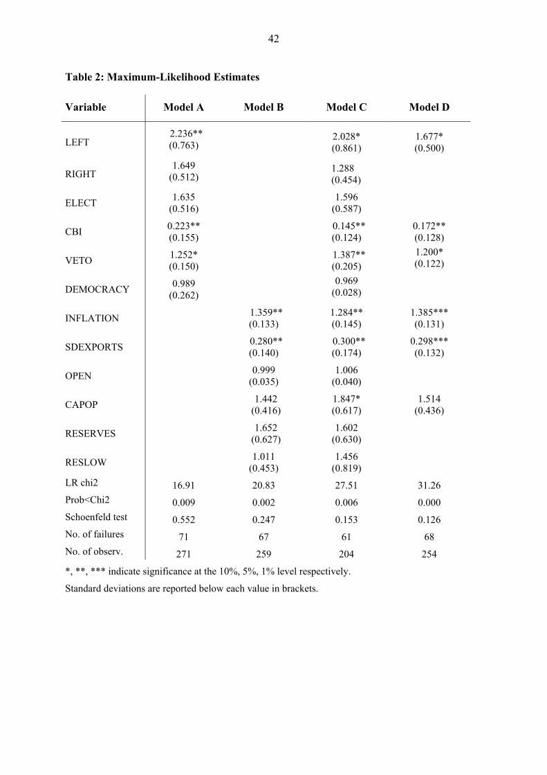
42

Table 2: Maximum-Likelihood Estimates

Variable Model A Model B Model C Model D

LEFT 2.236** (0.763) 2.028*

(0.861) 1.677* (0.500)

RIGHT 1.649

(0.512) 1.288 (0.454)

ELECT 1.635 (0.516)

1.596 (0.587)

CBI 0.223** (0.155)

0.145** (0.124)

0.172** (0.128)

VETO 1.252* (0.150)

1.387** (0.205)

1.200* (0.122)

DEMOCRACY 0.989 (0.262)

0.969 (0.028)

INFLATION 1.359** (0.133)

1.284** (0.145)

1.385*** (0.131)

SDEXPORTS 0.280** (0.140)

0.300** (0.174)

0.298*** (0.132)

OPEN 0.999 (0.035)

1.006 (0.040)

CAPOP 1.442 (0.416)

1.847* (0.617)

1.514 (0.436)

RESERVES 1.652 (0.627)

1.602 (0.630)

RESLOW 1.011 (0.453)

1.456 (0.819)

LR chi2 16.91 20.83 27.51 31.26 Prob<Chi2 0.009 0.002 0.006 0.000 Schoenfeld test 0.552 0.247 0.153 0.126 No. of failures 71 67 61 68 No. of observ. 271 259 204 254

*, **, *** indicate significance at the 10%, 5%, 1% level respectively.

Standard deviations are reported below each value in brackets.

43

Table 3: Calculation of Akaike Information Criterion (AIC)

Log likelihood q c AIC

Model A -142.202 6 1 298.404

Model B -134.639 6 1 283.278

Model C -101.178 12 1 228.356

Model D -129.689 6 1 273.378

Figure 4: Cumulative hazard functions of Cox-Snell residuals

a) Model A

0.5

11.

52

2.5

Nel

son-

Aal

en c

umul

ativ

e ha

zard

0 .5 1 1.5partial Cox-Snell residual

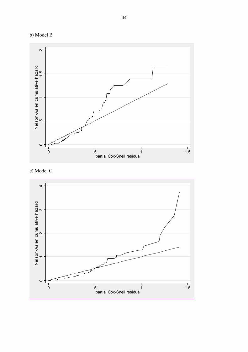
44

b) Model B 0

.51

1.5

2N

elso

n-A

alen

cum

ulat

ive

haza

rd

0 .5 1 1.5partial Cox-Snell residual

c) Model C

01

23

4N

elso

n-A

alen

cum

ulat

ive

haza

rd

0 .5 1 1.5partial Cox-Snell residual

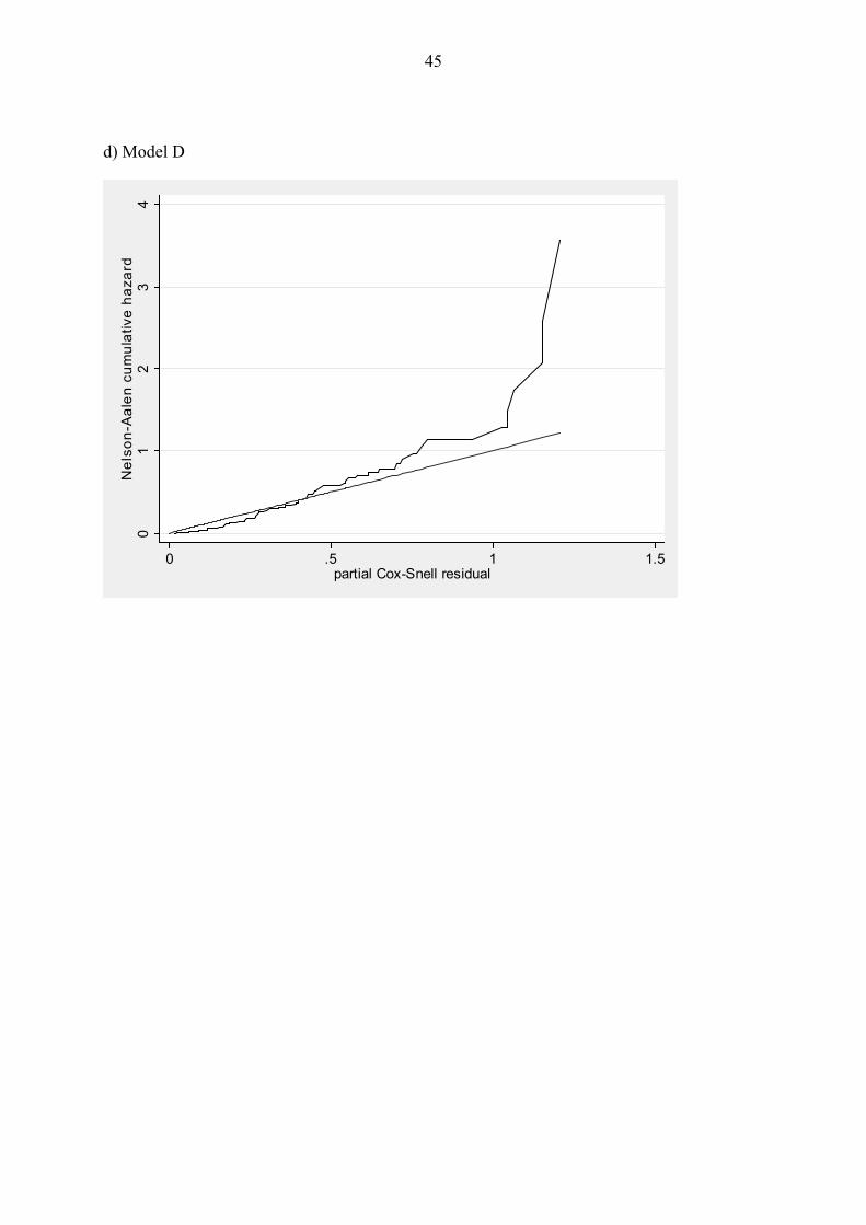
45

d) Model D 0

12

34

Nel

son-

Aal

en c

umul

ativ

e ha

zard

0 .5 1 1.5partial Cox-Snell residual