The Polar Coordinate System - University of Nebraskaâ€“Lincoln

University of Nebraska - LincolnDigitalCommons@University of Nebraska - Lincoln

MAT Exam Expository Papers Math in the Middle Institute Partnership

7-2008

The Polar Coordinate SystemAlisa FavingerUniversity of Nebraska-Lincoln

Follow this and additional works at: http://digitalcommons.unl.edu/mathmidexppap

Part of the Science and Mathematics Education Commons

This Article is brought to you for free and open access by the Math in the Middle Institute Partnership at DigitalCommons@University of Nebraska -Lincoln. It has been accepted for inclusion in MAT Exam Expository Papers by an authorized administrator of DigitalCommons@University ofNebraska - Lincoln.

Favinger, Alisa, "The Polar Coordinate System" (2008). MAT Exam Expository Papers. 12.http://digitalcommons.unl.edu/mathmidexppap/12

http://digitalcommons.unl.edu?utm_source=digitalcommons.unl.edu%2Fmathmidexppap%2F12&utm_medium=PDF&utm_campaign=PDFCoverPages

http://digitalcommons.unl.edu/mathmidexppap?utm_source=digitalcommons.unl.edu%2Fmathmidexppap%2F12&utm_medium=PDF&utm_campaign=PDFCoverPages

http://digitalcommons.unl.edu/mathmiddle?utm_source=digitalcommons.unl.edu%2Fmathmidexppap%2F12&utm_medium=PDF&utm_campaign=PDFCoverPages

http://digitalcommons.unl.edu/mathmidexppap?utm_source=digitalcommons.unl.edu%2Fmathmidexppap%2F12&utm_medium=PDF&utm_campaign=PDFCoverPages

http://network.bepress.com/hgg/discipline/800?utm_source=digitalcommons.unl.edu%2Fmathmidexppap%2F12&utm_medium=PDF&utm_campaign=PDFCoverPages

http://digitalcommons.unl.edu/mathmidexppap/12?utm_source=digitalcommons.unl.edu%2Fmathmidexppap%2F12&utm_medium=PDF&utm_campaign=PDFCoverPages

The Polar Coordinate System

Alisa Favinger Cozad, Nebraska

In partial fulfillment of the requirements for the Master of Arts in Teaching with a Specialization in the Teaching of Middle Level Mathematics in the Department of Mathematics.

Jim Lewis, Advisor

July 2008

Polar Coordinate System ~ 1

Representing a position in a two-dimensional plane can be done several ways. It

is taught early in Algebra how to represent a point in the Cartesian (or rectangular) plane.

In this plane a point is represented by the coordinates (x, y), where x tells the horizontal

distance from the origin and y the vertical distance. The polar coordinate system is an

alternative to this rectangular system. In this system, instead of a point being represented

by (x, y) coordinates, a point is represented by (r, θ) where r represents the length of a

straight line from the point to the origin and θ represents the angle that straight line

makes with the horizontal axis. The r component is commonly referred to as the radial

coordinate and θ as the angular coordinate. Just as in the Cartesian plane, the polar plane

has a horizontal axis and an origin. In the polar system the origin is called the pole and

the horizontal axis, which is a ray that extends horizontally from the pole to the right, is

called the polar axis. An illustration of this can be seen in the figure below:

r


In the figure, the pole is labeled (0, θ) because the 0 indicates a distance of 0 from the

pole, so (0,θ ) will be exactly at the pole regardless of the angle θ . The units of θ can be

given in radians or degrees, but generally is given in radians. In this paper we will use

both radians and degrees. To translate between radians and degrees, we recall the

conversion rules:

To convert from radians to degrees, multiply by π

180

To convert from degrees to radians, multiply by 180π

Plotting points on the polar plane and multiple representations

For any given point in the polar coordinate plane, there are multiple ways to

represent that point (as opposed to Cartesian coordinates, where point representations are

unique). To begin understanding this idea, one must consider the process of plotting

points in the polar coordinate plane. To do this in the rectangular plane one thinks about

moving horizontally and then vertically. However, in the polar coordinate plane, one

uses the given distance and angle measure instead. Although the distance is given first, it

is easier to use the angle measure before using the given distance.


The figure above is a picture of a polar coordinate system with degrees in black and

radians in green. This is just one example of what a polar coordinate plane may look

like; other examples may have additional or fewer angle measures marked. From this

figure it is easy to see why it may be called the polar system; it resembles what one might

see looking down on the north (or south) pole with visible longitudinal and latitude lines.

To plot the polar point (2, 60°), first the positive, or counter-clockwise, angle of 60˚ from

the polar axis is located, then a distance of 2 units along that angle is determined. The

location of this point is shown in green below:

2пп

п/6

п/32п/3

5п/6

7п/6

4п/33п/2

5п/3

11п/6

п/2


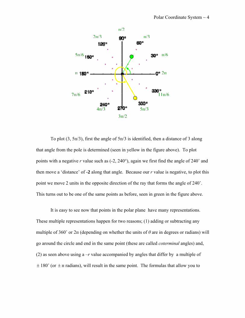
To plot (3, 5п/3), first the angle of 5п/3 is identified, then a distance of 3 along

that angle from the pole is determined (seen in yellow in the figure above). To plot

points with a negative r value such as (-2, 240°), again we first find the angle of 240˚ and

then move a ‘distance’ of -2 along that angle. Because our r value is negative, to plot this

point we move 2 units in the opposite direction of the ray that forms the angle of 240˚.

This turns out to be one of the same points as before, seen in green in the figure above.

It is easy to see now that points in the polar plane have many representations.

These multiple representations happen for two reasons; (1) adding or subtracting any

multiple of 360˚ or 2п (depending on whether the units of θ are in degrees or radians) will

go around the circle and end in the same point (these are called coterminal angles) and,

(2) as seen above using a –r value accompanied by angles that differ by a multiple of

± 180˚ (or ± п radians), will result in the same point. The formulas that allow you to

2пп

п/6

п/32п/3

5п/6

7п/6

4п/33п/2

5п/3

11п/6

п/2


create multiple representations of a single point in a polar plane are organized in the table

below:

Original representation New representation in degrees New representation in radians

(r, θ) (r, θ ± 360n); n = 1, 2, 3… (r, θ ± 2nп); n = 1, 2, 3…

(r, θ) (-r, θ± (2n+1)180); n = 1, 2, 3… (-r, (2n+1)п); n = 1, 2, 3…

In these formulas n can represent any integer, thus there are infinitely many

representations for any point in the polar coordinate system. Because mathematicians do

not want to worry about multiple representations, it is not unusual to impose the

following limits on r and θ to create unique representations: r ≥ 0 and θ is in the interval

[0, 360°) or (−180°, 180°] or, in radian measure, [0, 2π) or (−π, π].

Converting between rectangular and polar coordinates

Because both the rectangular and the polar coordinate systems exist, it is

important to be able to convert both points and equations from one system to the other .

These conversions are important because often times certain equations are best fit or

better represented in only one of these systems. If the plane of these two systems were

superimposed on one another, such that the pole coincides with the origin and the polar

axis coincides with the positive x-axis, any point P in this new plane can be assigned

either the polar coordinates (r, θ) or the rectangular coordinates (x, y). The following

four equations show the relationships between the polar coordinates (r, θ) and the

rectangular coordinates (x, y) of any point P when the two planes are superimposed:


i) x = r cos θ

ii) y = r sin θ

iii) r2 =x2 +y2

iv) xy

=θtan , x ≠ 0

Note: If x = 0 and y ≠ 0, that would mean that θ=90˚ or -90˚, where tangent is undefined.

Understanding how the first and second equations were established requires a

recollection of prior experiences with trigonometry. It is important to note here that

although the following examples deal with points found in the first quadrant, these four

equations can be used to convert a point found in any quadrant.

θ

θ

sin

sin

ryry

=

= and

θ

θ

cos

cos

rxrx

=

=

The formula to convert from a polar coordinate to a rectangular coordinate is:

P(x, y) = ( θcosrx = , θsinry = )

r

θ

P

x

y

P


Another way to think about this conversion is to recall the unit circle. On the unit circle,

any point can be represented by (cos θ, sin θ). Since the r value, or radial distance, on the

unit circle is 1, this is a special case of the general representation (r cos θ, r sin θ), which

is true for any value of r.

The following is an example of going through the process of converting a polar

coordinate pair to a rectangular coordinate pair. Using the above conversion formula the

polar coordinates (8, 30˚) are converted to rectangular coordinates as follows:

34

238

30cos8cos

=

⎟⎟⎠

⎞⎜⎜⎝

⎛=

==

x

x

xrx θ

4218

30sin8sin

=

⎟⎠⎞

⎜⎝⎛=

==

y

y

yry θ

Thus the rectangular coordinates that correspond with the polar coordinates of (8, 30˚) are

(4 3 , 4).

The following example will help to explain the conversion process from

rectangular coordinates to polar coordinates. If the (x, y) coordinates of the point P in the

figure below are (3,4) what are the polar coordinates, (r, θ), of this point? The use of the

Pythagorean Theorem will help to calculate r:

525

432

222

±==

+=

rrr

While the equation r2 = 25 has two solutions, we choose r = 5 so that r ≥ 0.

r

θ

P(3,4)→(r,θ)

3

4


To help find θ, we rely on trigonometric ratios. Information regarding the sides

opposite and adjacent to θ is given, so the tangent ratio can be used to help calculate θ:

°≈

=

=

=

−

5334tan

34tan

tan

1

θ

θ

θ

θxy

Thus, for this problem, θ is approximately 53˚.

With the calculations above it was found that the point (3, 4), represented as a

horizontal distance of 3 and vertical distance of 4, can be represented as (5, 53˚), a

straight line distance of 5 units from the pole, with that straight line forming an angle of

53˚ with the polar axis. To change any point (x, y) in the first or fourth quadrant from

rectangular coordinates to polar coordinates use the following formulas:

),( θr = )tan,( 122

xyyx −+

Note: The range of the inverse tangent function is -90˚< θ <90˚. Thus, when converting

from rectangular form to polar form, one must pay careful attention because using the

inverse tangent function confines the converted angle measures to only the first or fourth

quadrant. However, we can still use the formula identified above by adding or

subtracting 180o to the result. This is demonstrated in the following example in which we

convert the point (-3, 5) to polar coordinates:


),( θr =

( )°−

⎟⎠⎞

⎜⎝⎛

−+−

+

−

−

59,34

35tan,5)3(

)tan,(

122

122

xyyx

Observe that the point (-3, 5) is in the 2nd quadrant and -59˚ is in the fourth quadrant.

Points in the second and fourth quadrant are separated by 180˚, so to find the correct θ we

need to add (or subtract) 180 to -59 (-59+180 = 121). The polar coordinates that

correspond with the rectangular coordinates of (-3, 5) are ( °121,34 ).

Converting equations between rectangular and polar systems

Now, let us extend the idea of converting points between systems to converting

equations between systems. Equation conversion between systems is done because the

equations for some graphs are easier to represent in the rectangular system while the

equations of other graphs are represented more simply in the polar system. To do this,

we will begin by discussing some very simple rectangular equations and their

corresponding polar equations:

Rectangular equation Conversion process Polar equation

x = 3 r cos θ = 3 → θcos

3=r

y = 3 r sin θ = 3 → θsin

3=r


It is easy to see from the table, that a constant function in rectangular coordinates is a

more complicated function in polar coordinates. The opposite is true if we start with a

constant function in polar coordinates.

Polar equation Conversion process Rectangular equation

r = 3 r2 = 32 → x2 + y2 = 9

θ = 6π

x=r cos θ and y=r sin θ

x=r cos ⎟⎠⎞

⎜⎝⎛

6π y=r sin ⎟

⎠⎞

⎜⎝⎛

6π

32

23

23

xr

xr

rx

=

⎟⎟⎠

⎞⎜⎜⎝

⎛=

⎟⎟⎠

⎞⎜⎜⎝

⎛=

yr

yr

ry

221

21

=

⎟⎠⎞

⎜⎝⎛

=

⎟⎠⎞

⎜⎝⎛=

322 xy =

3xy =

From this table, it is easy to see that polar equations involving only constants aremore

simply represented as polar equations than as rectangular equations.

Converting rectangular equations to polar equations is quite simple. Recall that x

= r cos θ and y = r sin θ. By using this information, the polar equation that corresponds

with the rectangular equation of 3x – y + 2 = 0 can be found. First, begin by substituting


the polar values for x and y. Second, solve for r because polar equations are often

written in function format, with r as a function of θ:

θθ

θθθθ

sincos32

2)sincos3(02)sin()cos(3

023

−−

=

−=−=+−

=+−

r

rrr

yx

A simpler rectangular function is y = x. Converting this rectangular function to a polar

function and then plotting it on a polar plane is shown below:

°==

=

==

451tan

1cossin

cossin

θθθθ

θθ rrxy

Since the polar function is tan θ = 1, and we know that the tangent of 45˚ equals 1 (or

tan-1 1=45°),for any radial value r, the point (r, 45˚) will satisfy this polar function. A

graph of this equation in the polar plane is below:

2пп

п/6

п/32п/3

5п/6

7п/6

4п/33п/2

5п/3

11п/6

п/2tanθ =1


Another example of converting the common, but slightly more complex,

rectangular function y = x2 to a polar equation is shown below:

r

rrrrrr

xy

=

=

•=

=

=

θθθθ

θθ

θθ

2

22

22

2

2

cossin

cossin

cossin)cos(sin

Thus the rectangular equation y = x2 coincides with the polar equation θθ

2cossin

=r .

Now that we have a polar function, we can use a table to help us plot points:

θ in radians θ in degrees sin θ/cos2 θ (or r) (r, θ) θ in degrees

0 0 0 (0, 0)

п/6 30 0.6667 (.6667, 30)

п/4 45 1.4142 (1.4142, 45)

п/3 60 3.4641 (3.4641, 60)

п/2 90 undefined undefined

2п/3 120 3.4641 (3.4641, 120)

3п/4 135 1.4142 (1.4142, 135)

5п/6 150 0.6667 (0.6667, 150)

П 180 0 (0, 0)

7п/6 210 -0.6667 (-0.6667, 210)

5п/4 225 -1.4142 (-1.4142, 225)

4п/3 240 -3.4641 (-3.4641, 240)


3п/2 270 undefined undefined

5п/3 300 -3.4641 (-3.4641, 300)

7п/4 315 -1.4142 (-1.4142, 315)

11п/6 330 -0.6667 (-0.6667, 330)

2п 360 0 (0, 0)

*Those highlighted in red are multiple representations of points in the top part of the table.

*As shown in the table, when θ = 90˚ or θ = 270˚, this function is undefined. Thus the

domain for this equation excludes those values of θ for which cos θ = 0.

The points from the table are plotted in polar plane below. They are plotted using

the methods previously described. The coordinate plane with the function y = x2 overlays

the polar plane and it is apparent that this function connects the points from the table.

The function looks the same (a parabola) on both the rectangular and polar planes:


Converting from rectangular equations to polar equations, as mentioned above, is quite

simple because substitutions for the polar values of x and y can be used where they are

found in the rectangular equation. To graph those polar equations, a calculator or

graphing program can be used, or just as in algebra, we can create a table of values to

obtain the points that will be plotted.

Converting from a polar equation to a rectangular equation can be more difficult.

This is because in this situation limited substitutions are available to be made (in

particular, there is no explicit formula for θ in terms of x and y). Remember that

xy

=θtan and 222 yxr += . In the polar equation an r2 must be present to be able to

replace it with an x2 + y2 and a tan θ must be present in the polar equation to be able to

substitute it with xy . The substitutions used before in converting can also be used; r cos

θ in a polar equation can be substituted with x and r sin θ can be substituted with y.

As a first example of this process we begin with the polar equation r = 2. This

means that for any angle, the radial measure is 2. Intuitively, it is known that this will

create a circle on the polar plane with a radius of 2, but how can we change the polar

equation r = 2 into a rectangular equation? Remember the limited substitutions above;

there is not a simple substitute for r, so some manipulation should be done first to obtain

a value that can be substituted:

44

2

22

2

=+

=

=

yxrr


Now it can be seen that it is indeed an equation of a circle in the rectangular plane with a

radius of 2 and center at the origin.

For a second example of this conversion process we again begin with a fairly

simple polar equation: θ = 76˚. Intuitively it is known that this would be a straight line

in the polar plane at the angle 76˚, but what is the rectangular equation for that line?

Again some manipulation will need to be done in order to find that equation:

θ = 76˚

tan θ = tan 76˚.

tan θ = 4


xyxy

4

4

=

=

From the rectangular equation we can see that it is indeed the line that passes through the

origin with a slope of 4.

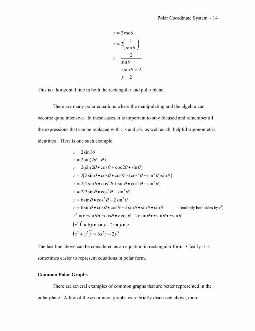
Now an example of conversion that is not quite as simple: r= 2 csc θ. Here the

manipulations are a little more complex because not only do we need to remember the

substitutions we can make, but we also must remember the relationship between

cosecant and sine:


22sin

sin2

sin12

csc2

==

=

⎟⎠⎞

⎜⎝⎛=

=

yr

r

r

r

θθ

θ

θ

This is a horizontal line in both the rectangular and polar plane.

There are many polar equations where the manipulating and the algebra can

become quite intensive. In these cases, it is important to stay focused and remember all

the expressions that can be replaced with x’s and y’s, as well as all helpful trigonometric

identities . Here is one such example:

( )( ) 32222

22

4

32

32

322

22

26

26

sinsinsin2coscossin6sinsinsin2coscossin6

sin2cossin6)sincossin3(2

)sincossincossin2(2]sin)sin(coscoscossin2[2

)sin2coscos2(sin2)2sin(2

3sin2

yyxyx

yyyxxyr

rrrrrrrrrrrrrrr

−=+

••−••=

••−••=

••−••=−•=

−•=

−•+•=

−+••=

•+•=+=

=

θθθθθθ

θθθθθθθθθ

θθθ

θθθθθ

θθθθθθ

θθθθθθ

θ

The last line above can be considered as an equation in rectangular form. Clearly it is

sometimes easier to represent equations in polar form.

Common Polar Graphs

There are several examples of common graphs that are better represented in the

polar plane. A few of these common graphs were briefly discussed above, more

(multiply both sides by r3)


examples in greater detail will follow. The table that follows displays some of these

examples in a very basic manner.

Basic Equation Name of Graph Basic shape of Graph

θsin1=r

Circle

θar =

Archimedean spiral

)cos1(1 θ±=r

Cardioid “heart”

θcos21±=r

Limaçon

θ5sin3=r

Rose

θcos422 =r

Lemniscate


Circles

I. ar = . This equation indicates that no matter the angle, the distance from the origin

must be a. To sketch the graph, one can take )360,0[ °∈θ as the domain. Recall r = 2

(discussed previously) was an example of a circle in this form.

II. θcos2ar = . This is a circle of radius |a| with center at (a, 0), on the x-axis. Note

that a might be negative and so the absolute value bars are required on the radius. They

should not be used, however, on the center. To sketch the graph, one can use the

domain of )180,0[ °∈θ . The equation r = -8 cos θ has an a value of -4 because 2(-4)=-8,

and therefore this circle would have a radius of 4 and a center at (-4,0).

III. θsin2br = . This is similar to the previous example. It is a circle of radius |b| and

center (0,b) on the y-axis.

r=2(2) cos θ r=2(3) sin θ


Spirals

I. Archimedean spiral, r = aθ. As |a| increases the spiral spreads out and as |a| decreases

the spiral compresses. The graph of the spiral turns about the origin, crossing the y-axis

as the expression aθ changes signs.

The graph is sketched for domain ),0[ ∞∈θ . If negative values of θ are included

in the domain, the reflection of this graph about the y-axis is also obtained.

II. Equiangular spiral, r = eaθ. Again as |a| increases or decreases the spiral expands or

compresses respectively. The spiral crosses the x-axis as the sign of a changes.


Cardioids

The domain needed to sketch these graphs is (0, 360] or (0, 2π].

The equation )sin1( θ±= ar or )cos1( θ±= ar will produce what is referred to as a

cardioid. These graphs have a shape that is similar to a heart and always contain the

origin. As |a| increases or decreases the “heart” shape expands or compresses. A way to

look at the role of cos and sin in the polar world is to think about symmetry. There are

ways to test for symmetry, but those are not necessary if the following fact is known. If

cos is used the axis of symmetry is the x-axis and if sin is used the axis of symmetry is

the y-axis. Changes in the sign of the expression will reflect the cardioid over the axis of

symmetry.

r=2(1-sin θ)

r=2.5(1+cos θ)


Limaçons

The domains needed to sketch these graphs is (0, 360] or (0, 2π].

I. Limaçons with an inner loop: θcosbar ±= and θsinbar ±= . If |a/b|<1 (|b |is

greater than |a|) , these graphs will look similar to cardioids with an inner loop and will

always contain the origin. Similar to cardioids, the rules of symmetry using cos or sin

apply here. As b changes signs the limaçon is reflected of the x or y axis. As |b| gets

larger while |a| stays fixed, the size of the body expands, whereas as |a| gets smaller and

|b| stays fixed, the size of the inner loop increases.

II. Limaçons with a dimple: θcosbar ±= and θsinbar ±= . If 1<|a/b|<2 , these

graphs do not have an inner loop and do not contain the origin. The constant b plays the

same role as before, expanding the body as |b| increases as well as reflecting the graph

over the axis of symmetry if the sign of b is changed. The constant a in this case

determines the size of the “dimple” rather than the inner loop as before. Again cos and

r=1+2 cos θ

r=1-4sin θ


sin determine how the limaçon lays (which axis is the axis of symmetry). These graphs

look similar to cardioids.

III. Convex limaçons: θcosbar ±= and θsinbar ±= . If |a/b|≥ 2, the dimple disappears

completely and a convex limaçon appears and where there would have been a dimple,

there is a vertical or horizontal line, as |a/b| gets larger and larger this vertical or

horizontal line becomes smaller and smaller. The same rules for b (expanding or

compressing and opposite signs reflecting) and cos/sin (axis of symmetry) apply here as

well.

r=3+2 sin θ

r=1.5-1.25 cos θ

r=3-1.5 cos θ

r=10+3 sin θ


Roses

My favorite polar graphs are the rose graphs. The same rules for symmetry apply to

these graphs as well. The general equation form for a rose graph is: )sin( θnar = or

)cos( θnar = , when n≥ 2 and an integer. If n is odd, there are n petals and the domain is

(0, π]. If n is even, there are 2n petals and the domain is (0, 2π]. The length of each petal

is |a|. If n=1, a circle is created with the center at the origin. If n is not an integer, the

graph is similar to a rose but the petals overlap.

3 cos (5.5t)

r=3sin(5θ) r=5cos(4θ)


Lemniscate

The equation θ2sin22 ar ±= or θ2cos22 ar ±= will produce the graph of a lemniscate, a

shape similar to a figure eight. The length of each “oval” (the top and bottom part of the

figure eight) is determined by |a|. Again, cos and sin determine how the lemniscates lays

on the plane.

Why use the polar system?

Obviously, from what is stated above, polar coordinates are most appropriate in

any context where what is being studied is tied to direction and length from a center

point. There are several real-life applications that fall into this kind of context. One of

the first references to polar coordinates is that of the astronomer Hipparchus who used

them to establish stellar positions. This idea leads us to the use of polar coordinates and

equations to help us understand the circular or orbital motion of many things in our

universe.

Polar coordinates are used often in navigation as well. The destination or

direction of travel can be given as an angle and a distance from the starting point. For

instance, aircrafts use a slightly modified version of the polar coordinates for navigation.

In this system, the one generally used for any sort of navigation, the polar axis is


generally called heading 360, and the angles continue in a clockwise direction, rather

than counterclockwise, as in the mathematical system. Heading 360 corresponds to

magnetic north, while headings 90, 180, and 270 correspond to magnetic east, south, and

west, respectively. Thus, an aircraft traveling 5 nautical miles due east will be traveling 5

units at heading 90. It is easy to see how this system corresponds with the polar

coordinate system.

Systems with radial or point forces are also good candidates for the use of the

polar coordinate system. These systems include gravitational fields and radio antennas.

Radially asymmetric systems may also be modeled with polar coordinates. For example,

a microphone's pickup pattern illustrates its proportional response to an incoming sound

from a given direction, and these patterns can be represented as polar curves. Three

dimensional polar modeling of loudspeaker output patterns can be used to predict their

performance.

In all of these situations where the polar system is applicable, it is easier to think

about these situations in polar terms rather than with a rectangular system. This is

because they lend themselves to using a distance and a direction much better than using

just vertical and horizontal directions.

Other coordinate systems

During my research over the polar coordinate system, I found examples of other

coordinate systems, some that I had heard of before and some that were new to me. I was

very surprised to learn that NASA uses a three dimensional coordinate system for each


space shuttle. But after thinking about it, it does make sense to have such a system in

place so that when astronauts are repairing the shuttle while in space, specific directions

can be given from here on Earth that enable the astronaut to find whatever needs to be

repaired quickly.

A more common such system is the geographic coordinate system. Generally,

one learns a simplified version of this system in geography classes. A geographic

coordinate system enables every location on the earth to be specified. There are three

coordinates: latitude, longitude and geodesic height. Most people are familiar with both

the ideas of latitude and longitude, but many are not familiar with geodesic height.

Latitude and longitude enable us to specify a location on a perfect sphere. Because the

Earth is not a perfect sphere, a third number is need to represent how far above or below

a point is located from the given latitude and longitude. The geodesic height does just

that. Generally, it represents the distance from sea-level at a given latitude and longitude.

In recent years, it seems that this geographic coordinate system has become very

useful. GPS (global positioning systems) devices use ideas behind the geographic

coordinate system. GPS systems are becoming more popular by the day. Many people

have them in their cars to help get from place to place, and I even have a watch with a

GPS that tells me how fast and far I am running.


References

Hungerford, Thomas W. (2004). Precalculus: A graphing approach. Austin, TX: Holt, Rinehart and

Winston.

Kim, Jiho (2007). GCalc, java mathematical graphing system. Retrieved June 24, 2008, from GCal 3 Web

site: http://gcalc.net/

Larson, Ron (2004). Precalculus. Boston, MA: Houghton Mifflin Company.

Larson, Ron (2002). Calculus I: With precalculus. Boston, MA: Houghton Mifflin Company.

Roberts, Lila F. Mathdemos project. Retrieved June 24, 2008, from Polar Gallery Web site:

http://mathdemos.gcsu.edu/mathdemos/family_of_functions/polar_gallery.html

Swokowski, Earl W. Calculus with analytic geometry. Boston, MA: PWS Kent Publishing Company.

Documents

The Polar Coordinate System - University of Nebraskaâ€“Lincoln