The POISSON and SUPERFIS H Suite H Suite - …pbpl.physics.ucla.edu/Education/Schools/USPAS_2004/SFISH...The POISSON and SUPERFISThe POISSON and SUPERFIS H Suite H Suite J.B. Rosenzweig

The POISSON and SUPERFISH SuiteThe POISSON and SUPERFISH Suite

J.B. Rosenzweig

UCLA Department of Physics and Astronomy

USPAS, 7/1/04

POISSON/SUPERFISH CapabilitiesPOISSON/SUPERFISH Capabilities

• SUPERFISH: axisymmetric rf cavitiesTM-mode frequency-domain analysis

Field profile

Frequency tuning

Power dissipation in walls

• POISSON: 2-D (axisymmetric and Cartesian)magnetostatics

Permeable materials

Magnetic multipole analysis

Permanent magnets (Amperian currents or PANDIRA)

Electrostatics!

• Shared input mesh, output format

• Input maps for UCLA PARMELA and HOMDYN

Mesh Setup for POISSON/SUPERFISHMesh Setup for POISSON/SUPERFISH

• Electromagnetic boundary problem described bydiscretized Maxwell (in Poisson or Helmoltz form)equations

• Solved by successive over-relaxation method

• Program AUTOMESH creates computational meshfrom geometric description

• Program LATTICE setups up difference equationsfor AUTOMESH grid points

Simple Example: Gun Half CellSimple Example: Gun Half Cell

• Half-cell geometry for old UCLA rf gun

• Can be seen as part of a periodic system (basis ofFourier description of linac structures)

• Illustrates boundary conditions

• Obtain 0- mode splitting

• Post-processing for graphical output

• Can calculate power dissipation profile, frequencytuning (for tuning cuts in gun)

AUTOMESH input for 0.6 cellAUTOMESH input for 0.6 cell

~/fish4> more halfcell.dat

X UCLA 2856MHz RF HALF CELL

$REG NREG=1,XMAX=3.0,YMAX=4.16,DX=0.03,NPOINT=8,YREG1=2.5$

$PO X=0.00,Y=0.000$

$PO X=0.00,Y=4.155$

$PO X=1.630,Y=4.155$

$PO X=1.630,Y=1.953$

$PO NT=2,X0=2.583,Y0=1.953,R=0.953,THETA=270.0$

$PO X=2.625,Y=1.000$

$PO X=2.625,Y=0.000$

$PO X=0.000,Y=0.000$

Title

• One region, defined by 8 points

• X and Y limits defined in first region

• DX is mesh spacing (DY defaults to DX)

• Points are joined by lines, circles, hyperbolae

• Region always ends back at initial point

All distances in cm

Run automesh and type in input file (halfcell.dat in ex.)

AUTOMESH Screen OutputAUTOMESH Screen Output

REGION NO. 1

LOGICAL BOUNDARY SEGMENT END POINTS

ISEG KB LB KD LD KE LE

1 1 1 0 1 1 161

2 1 161 1 0 55 161

3 55 161 1 -1 56 76

4 56 76 -1 -1 87 39

5 87 39 1 0 88 39

6 88 39 1 -1 88 1

7 88 1 -1 0 1 1

--- WARNING --- USER PROVIDED DRIVE POINT

COULD BE BETTER

THAN THE DEFAULT BEST GUESS DRIVE

POINT.

K is “x” index

L is “y” index

Drive point (center of SOR calc.)

May be important

AUTOMESH and meshing errorsAUTOMESH and meshing errors

• If the mesh is too coarse, and features of the

geometry are too fine, then AUTOMESH will

fail to generate a mesh and give an error —

you will then need to make the mesh finer

• Even though this feature enforces adequate

meshing, it is wise to check the convergence

of the problem (e.g. frequency in SUPERFISH)

to see if the mesh spacing affects the answer.

AUTOMESH graphical outputAUTOMESH graphical output

• Run psfplot (plotting

package)

• In psfplot, type “s” to all

prompts (“-1 s” to end)

• Outputs only the

geometry

• Simple check on work

after AUTOMESH

Running LATTICERunning LATTICE

• Inputs in blue

• Tape73 is default output fromAUTOMESH, input to LATTICE

• PROBLEM CON(stant)s dealingwith boundary conditions beginwith “*”, end with “s” (see p. 403for full listing

• The boundary conditions are, 21:upper, 22: lower, 23: right, 24: left(22-24 are in order)

• In SUPERFISH, 1 is anconducting boundary, 0 is amagnetic (symmetry) boundary.

• Tapes 35 and 36 are input forSUPERFISH

?type input file name (s for default)

tape73

BEGINNING OF LATTICE EXECUTION

DUMP 0 WILL BE SET UP FOR SUPERFIS

X UCLA 2856MHz RF HALF CELL

?TYPE INPUT VALUES FOR CON(?)

*21 1 0 0 1 S

ELAPSED TIME = 0.1 SEC.

GENERATION COMPLETED

DUMP NUMBER 0 HAS BEEN WRITTEN ON TAPE35.

DUMP NUMBER 0 HAS BEEN WRITTEN ON TAPE36.

LATTICE graphical outputLATTICE graphical output

• Check meshing…

• In sfo1, type “0 1 s” to firstprompt, “s”, “go”, and “-1 s”

• Outputs only the mesh

• Note that outside ofYREG1 (2.5 cm), the meshspacing has doubled

• Can also stretch x-spacing

Running SUPERFISHRunning SUPERFISH

• Run superfish

• tty is terminal input

• CON(65) is a guessfrequency in MHz - you willfind a different mode (ifpossible) when chosendifferently (only one in thisproblem)

• Convergence and finalfrequency are given inscreen output

?type "tty" or input file name

tty

?TYPE INPUT VALUE FOR DUMP NUM

0

BEGINNING OF SUPERFISH EXECUTION FROM

DUMP NUMBER 0

PROB. NAME = UCLA 2856MHz RF HALF CELL


*65 2856. s


CYCLE DEL(k**2) FREQ[MHz]

--------------------------------------

2856.00000

1 -4.2046E-04 2854.32373

2 -1.4901E-06 2854.31787

SOLUTION CONVERGED IN 2 ITERATIONS


DUMP NUMBER 1 HAS BEEN WRITTEN.


-1 s

PI-Mode Boundary ConditionsPI-Mode Boundary Conditions

• The CONs that are input to LATTICE

include a boundary condition card for

each boundary• For the -mode, CON(23) is 0

• To view graphically:

?TYPE INPUT DATA- NUM, ITRI, NPHI, INAP, NSWXY,

1 0 50 s

INPUT DATA

NUM= 1 ITRI= 0 NPHI= 50 INAP= 0 NSWXY= 0

PLOTTING PROB. NAME = UCLA 2856MHz RF HALF CELL CYCLE = 2

?TYPE INPUT DATA- XMIN, XMAX, YMIN, YMAX,

s

INPUT DATA

XMIN= 0.000 XMAX= 2.625 YMIN= 0.000 YMAX= 4.155

ARROW PLOT?: ENTER Y FOR YES OR N FOR NO

no

?TYPE GO OR NO

go


-1 s

(number of flux lines is 50)

Arrow plotsArrow plots

• Standard plot is not

E-field line, it is constant

enclosed flux surface (rH).

This can be confusing.

• Use arrow plot… ARROW PLOT?: ENTER Y FOR YES OR N FOR NO

y

ENTER NSKIP

10 (controls density, larger is less dense)

ENTER SCALING FACTOR

10 (controls arrow size)

?TYPE GO OR NO

go


-1 s Note high field near axis!

Output filesOutput files

• Each code in suite produces output filesoutaut

outlat

outpoi

• outaut and outlat contain problem setup info

• outfis contains solution information

• Post-processing of detailed solution information(dump 1) possible with sfo1

• More important in POISSON (outpoi gives usefulfield info directly)

Boundary analysis with SFO1Boundary analysis with SFO1

• Running sfo1 you can find:

Power dissipation (normalized

to peak accelerating field of 1

MeV/m)

Export to ANSYS for thermal

simulation?

Frequency tuning (cut

coefficients

Each segment listed

separately

?type "tty" or input file name

tty


1

BEGINNING OF SFO1 EXECUTION FROM DUMP NUMBER 1

PROB. NAME = UCLA 2856MHz RF HALF CELL


1

*50 7 *106 0.9999 S (106 is particle beta)

?TYPE INPUT VALUES FOR ISEG'S

1 2 3 4 5 6 7 S (all seven segments are listed (not necessary, 6 and 7 are

not valid)

---WARNING --- FREQUENCY PERTURBATION CALCULATION

CORRECT ON A CONDUCTOR ONLY

SFO1 OutputSFO1 Output

?TYPE GO FOR OUTPUT SUMMARY AT TERMINAL

go

1SUPERFISH General summary Tue Oct 1 08:52:33 2002

Total number of points = 11921 NCELL = 1 ZCTR = 0.0000 cm

LINT = 1 Average r = 0.0261 cm ZBEG = 0.0000 cm ZEND = 2.6250 cm

Integral [Ez(z,r= 0.03 cm)sin(Kz)dz] = 13394.55 V

Integral [Ez(z,r= 0.03 cm)cos(Kz)dz] = 20423.91 V

1SUPERFISH DTL summary Tue Oct 1 08:52:33 2002

Problem name = UCLA 2856MHz RF HALF CELL

SUPERFISH calculates the frequency [f] to at most six place accuracy

depending on the input mesh spacing.

Full cavity length [2L] = 5.2500 cm Diameter = 8.3100 cm

Mesh problem length [L] = 2.6250 cm

Full drift-tube gap [2g] = 3.2600 cm

Beta = 0.9999000 Proton energy = 65400.941 MeV

Frequency [f] (starting value =2856.000) = 2854.317871 MHz

Eo normalization factor (CON(74)=ASCALE) for 1.000 MV/m = 9124.7

Stored energy [U] for mesh problem only = 0.30303 mJ

Power dissipation [P] for mesh problem only = 572.75 W

Q (2.0*pi*f(Hz)*U(J)/P(W)) = 9488

Transit time factor [T] = 0.77805

Quality factor

Transit time factor

SFO1 Output (continued)SFO1 Output (continued)

Shunt impedance [Z] mesh problem only, ((Eo*L)**2/P) = 1.20307 Mohm

Shunt impedance per unit length [Z/L] = 45.831 Mohm/m

Effective shunt impedance per unit length [Z/L*T*T] = 27.745 Mohm/m

Magnetic field on outer wall = 2395 A/m

Hmax for wall and stem segments at z= 0.00,r= 3.28 cm = 2665 A/m

Emax for wall and stem segments at z= 1.66,r= 1.72 cm = 1.624 MV/m

Beta T Tp S Sp g/L Z/L

0.99989998 0.77805 0.12917 0.51027 0.11833 0.620952 45.831303

ISEG zbeg rbeg zend rend Emax*epsrel Power df/dz df/dr

(cm) (cm) (cm) (cm) (MV/m) (W) (MHz/mm)

Wall-----------------------------------------------------------------------Wall

1 0.0000 0.0000 0.0000 2.5000 1.4955 48.1330 43.9345 0.0000

2 0.0000 2.5000 0.0000 4.1550 0.9270 159.8759 -49.4446 0.0000

3 0.0000 4.1550 1.6300 4.1550 0.0020 169.1528 0.0000 -72.3290

4 1.6300 4.1550 1.6300 2.5000 0.9756 158.3179 -47.5337 0.0000

5 1.6300 2.5000 1.6300 1.9530 1.4212 26.1670 11.0253 0.0000

6 1.6300 1.9530 2.5830 1.0000 1.6237 11.1060 31.5280 15.0800

7 2.5830 1.0000 2.6250 1.0000 0.2704 0.0001 0.0000 0.0402

Wall----------------------------------- Total = 572.7526 --------------Wall


-1 s

Tuning cuts

(can break segments

up into smaller lengths)

Shunt impedance

(low for half-cell, it is

too wall-dominated)

To obtain power for actual case, multiply this by

where is the peak on-axis field in MV/m.

EmaxT( )2

Emax

Automating the problemAutomating the problem

• After you have set up theproblem in AUTOMESH andLATTICE, it is helpful to runthe entire problem with aLinux script

• Must chmod file to “x” to getit to run

• I use stout executables in~anderson/bin. We aremoving to standardize allexecutables on PBPLmachines

~/fish4> more halffish

automesh << MESHEND

halfcell.dat

MESHEND

lattice << LATTICEND

tape73

*21 1 0 0 1 S

LATTICEND

superfish << FISHEND

TTY

0

*65 2856. S

-1 S

FISHEND

sfo1 << SFOEND

tty

1

*50 7 *106 0.9999 S

1 2 3 4 5 6 7 S

GO

-1 S

SFOEND

psfplot << PLOTEND

A “real” problem: the 1.6 cell gunA “real” problem: the 1.6 cell gun

• Include beam tube

• High precision

• Can obtain zeromode…

• Detune for 0.6 and fullcell frequencies

• Need to includeperturbations due totuner/laser/vacuumports

stout:~/Newfish> more newgun

1superfish brookhaven gun

&reg xmin=00.,ymin=0.,xmax=15.0,ymax=4.21153,dx=0.05,npoint=17 &

&PO X=0.000,Y=0.000 &

&PO X=0.000,Y=4.1581 &

&PO X=2.27584,Y=4.1581 &

&PO X=2.27584,Y=2.20218 &

&PO NT=2,X0=3.22834,Y0=2.20218,R=0.9525,THETA=270.0 &

&PO X=3.2766,Y=1.24968 &

&PO X=3.3782,Y=1.24968 &

&PO X=3.4798,Y=1.24968 &

&PO X=3.52806,Y=1.24968 &

&PO NT=2,X0=3.52806,Y0=2.20218,R=0.9525,THETA=0.0 &

&PO X=4.48056,Y=4.2084 &

&PO X=7.73000,Y=4.2084 &

&PO X=7.73000,Y=2.20218 &

&PO NT=2,X0=8.68250,Y0=2.20218,R=0.9525,THETA=270.0 &

&PO X=10.68250,Y=1.24968 &

&PO X=10.68250,Y=0.000 &

&PO X=0.000,Y=0.000 &

1.6 cell gun output1.6 cell gun output

• Fields nearly balanced

• Need beam tube twice aperture in length

Traveling waves and boundary conditionsTraveling waves and boundary conditions

• Traveling wave mode characteristics are obtained by doingstanding wave problem, obtaining Fourier description(separate code)

• Use minimum symmetry (see /2 mode example) forproblem

Embedded region: PWT 0.5+0.5 cellEmbedded region: PWT 0.5+0.5 cell

• Minimal symmetryneeded to obtain 0and modes

• Embed the PWTdisks. Ignorecooling rods

1superfish pwt fullcell

$reg nreg=2, dx=0.025, npoint=5, xmax=5.248, ymax=5.5 $

$po x=0.0, y=0.0 $

$po x=0.0, y=5.5 $

$po x=5.248, y=5.5 $

$po x=5.248, y=0.0 $

$po x=0.0, y=0.0 $

$reg npoint=10, mat=0, ibound=1 $

$po x=2.624, y=4.2525 $

$po x=2.221, y=4.2525 $

$po nt=2, x0=2.221, y0=4.0525, r=0.2, theta=180.0 $

$po x=2.021, y=1.3 $

$po nt=2, x0=2.521, y0=1.3, r=0.5, theta=270.0 $

$po x=2.727, y=0.8 $

$po nt=2, x0=2.727, y0=1.3, r=0.5, theta=360.0 $

$po x=3.227, y=4.0525 $

$po nt=2, x0=3.027, y0=4.0525, r=0.2, theta=90.0 $

$po x=2.624, y=4.2525 $

PWT outputsPWT outputs

CON(23)=0, CON(24)=1 CON(23)=1, CON(24)=1Note mode separation!

Original guess was 1900 MHz

Hybrid TW/SW gunHybrid TW/SW gun

Standing wave gun section

Coupling cell

TW section (first half period)

Rendered cartoon of device

(opposite direction)

POISSONPOISSON

• Static “potential” problems

• Shares input setup

• CONs are more important in latticeCylindrical v. cartesian symmetry

Output fields

Harmonic field analysis

• Permanent magnets with Amperian currentsUndulators

Permanent magnet hybrid quads

• Electrostatic problems

Example: Standard PBPL quadExample: Standard PBPL quad

• Input deck has

magnetic material

$reg nreg=4, dx=0.1, xmax=15.0, ymax=15.0, xreg1=8.0, yreg1=8.0., npoint=5$

$po y= 0.00, x= 0.00$

$po y=15.00, x= 0.00$

$po y=15.00, x=15.00$

$po y= 0.00, x=15.00$

$po y= 0.00, x= 0.00$

$reg mat=2, npoint=19$

$po x=0.000, y=10.795$

$po x=0.000, y=12.70$

$po x=3.393, y=12.70$

$po x=12.70, y=3.393$

$po x=12.70, y=0.00$

$po x=10.795, y=0.00$

$po x=10.795, y=2.604$

$po x=7.710, y=5.689$

$po x=4.567, y=2.546$

$po x=6.026, y=1.087$

$po x=5.397, y=0.458$

$po x=.118, y=.588, x0=4.901, y0=.121, nt=2$

$po y=5.019, x=.709, r=2.668 nt=3$

$po x=0.337, y=.496, x0=0.121, y0=4.901, nt=2$

$po x=1.087, y=6.026$

$po x=2.546, y=4.567$

$po x=5.689, y=7.710$

$po x=2.604, y=10.795$

$po x=0.000, y=10.795$

$reg mat=1, cur=-1835., npoint=5$

$po x=4.521, y=8.877$

$po x=5.689, y=7.710$

$po x=2.547, y=4.568$

$po x=1.379, y=5.734$

$po x=4.521, y=8.877$

$reg mat=1, cur=1835., npoint=5$

$po x=7.710, y=5.689$

$po x=8.877, y=4.521$

$po x=5.734, y=1.379$

$po x=4.568, y=2.547$

$po x=7.710, y=5.689$

(continued)

mat=2 means internal

permeability curve

mat=1 means conductor (cur is current in amps)

nt=2 is arc,

nt=3 hyperbola

Complex representation of fieldComplex representation of field

• Standard analysis in cylindrical coordinates

• Allows harmonic analysis of POISSON output

Bx iBy = inr

rnorm

n 1

n=1

cnrnorm

exp i n 1( )[ ]

Bx iBy = Bm

n= 0

exp im( )or

Bm =m + 1

rnorm

r

rnorm

m

bm+1 iam+1( )with

Standard quad scriptStandard quad script

automesh << MESHEND

quad.2

MESHEND


tape73

*21 0 1 0 1 *81 1 s

LATTICEND

poisson << POISEND

tty

0 s

*19 0 *6 0 *46 4 *38 0.0 *110 5 50 1.0 90. 1. *85 1e-5 1e-5 s

-1

POISEND

psfplot << PLOTEND

1 0 20 s

s

go

-1 s

PLOTEND

As usual, CON(21)-(24) gives symmetry. For quad

you need lower and left to have field normal to

bdry (CON is 1).

CON(6) is permeability option. Value of 0 indicatesthat permeability is finite (w/mat=2 derives µ from

standard table).

These symmetries are also declared in CON(46),

which governs harmonic analysis of fields (4 means

symmetrical quad)

CON(110) is the number of harmonic terms, (111)

is points on the analysis circle,

(112) is the radius of circle, (113) is the angle in

degrees of analysis (114) is normalization radius.

CON(19) is coordinate system (0 is Cartesian)

Standard quad outputStandard quad output

• No saturation

• Pole piece flaring

• Good field quality? Look atoutpoi

Harmonic analysis

OUTPOI fileOUTPOI file

• At end of outpoi, findharmonic analysis

• Only harmonics allowedby symmetry arecalculated

Quadrupole

Dodecapole

• Field maps alsooutput…

1TABLE FOR VECTOR POTENTIAL COEFFICIENTS

0NORMALIZATION RADIUS = 1.00000

0 A(X,Y) = RE( SUM (AN + I BN) * (Z/R)**N )

0 N AN BN ABS(CN)

0 2 3.1634E+02 0.0000E+00 3.1634E+02

0 6 7.1072E-03 0.0000E+00 7.1072E-03

0 10 6.9814E-03 0.0000E+00 6.9814E-03

0 14 5.4019E-03 0.0000E+00 5.4019E-03

0 18 4.7405E-03 0.0000E+00 4.7405E-03

1TABLE FOR FIELD COEFFICIENTS

0NORMALIZATION RADIUS = 1.00000

0 (BX - I BY) = I * SUM N*(AN + I BN)/R * (Z/R)**(N-1)

0 N N(AN)/R N(BN)/R ABS(N(CN)/R)

0 2 6.3269E+02 0.0000E+00 6.3269E+02

0 6 4.2643E-02 0.0000E+00 4.2643E-02

0 10 6.9814E-02 0.0000E+00 6.9814E-02

0 14 7.5627E-02 0.0000E+00 7.5627E-02

0 18 8.5329E-02 0.0000E+00 8.5329E-02

Example: Neptune solenoidExample: Neptune solenoid

• Double coil solenoid

• Cylindrical symmetry

• Note here x -> r, y -> z.

• Need to obtain field

maps for PARMELA

and HOMDYN

double solenoid

$reg nreg=5,xmax=20.00,ymax=60.00,ktop=5,ltop=50,dx=0.25,dy=0.25,npoint=5$

$po x=0.000,y=0.000$

$po x=20.000,y=0.000$

$po x=20.000,y=60.000$

$po x=0.000,y=60.000$

$po x=0.000,y=0.000$

$reg mat=1, cur=20000, npoint=5$

$po x=5.1,y=21.35$

$po x=10.2,y=21.35$

$po x=10.2,y=29.8$

$po x=5.1,y=29.8$

$po x=5.1,y=21.35$

$reg mat=2,npoint=9$

$po x=3.6,y=21.35$

$po x=10.2,y=21.35$

$po x=10.2,y=29.8$

$po x=4.4,y=29.8$

$po x=4.4,y=32.34$

$po x=12.74,y=32.34$

$po x=12.74,y=18.81$

$po x=3.6,y=18.81$

$po x=3.6,y=21.35$


$po x=5.1,y=32.34$

$po x=10.2,y=32.34$

$po x=10.2,y=40.79$

$po x=5.1,y=40.79$

$po x=5.1,y=32.34$


$po x=12.74,y=32.34$

$po x=12.74,y=43.33$

$po x=4.4,y=43.33$

$po x=4.4,y=40.79$

$po x=10.2,y=40.79$

$po x=10.2,y=32.34$

$po x=12.74,y=32.34$

Solenoid scriptSolenoid script

• Note boundaries

• No bucking coil - can

translate field map in

PARMELA/HOMDYN

• CON(42-45) gives K

min/max, L min/max for

field map (lineout for on-

axis field)

automesh << MESHEND

doublesol

MESHEND


s

*6 0 *19 1 *21 0 0 0 0 s

LATTICEND

poisson << POISSONEND

tty

0

*42 1 1 1 241 s

-1 s

POISSONEND

psfplot << PLOTEND

1 0 20 s

s

go

-1 s

PLOTEND

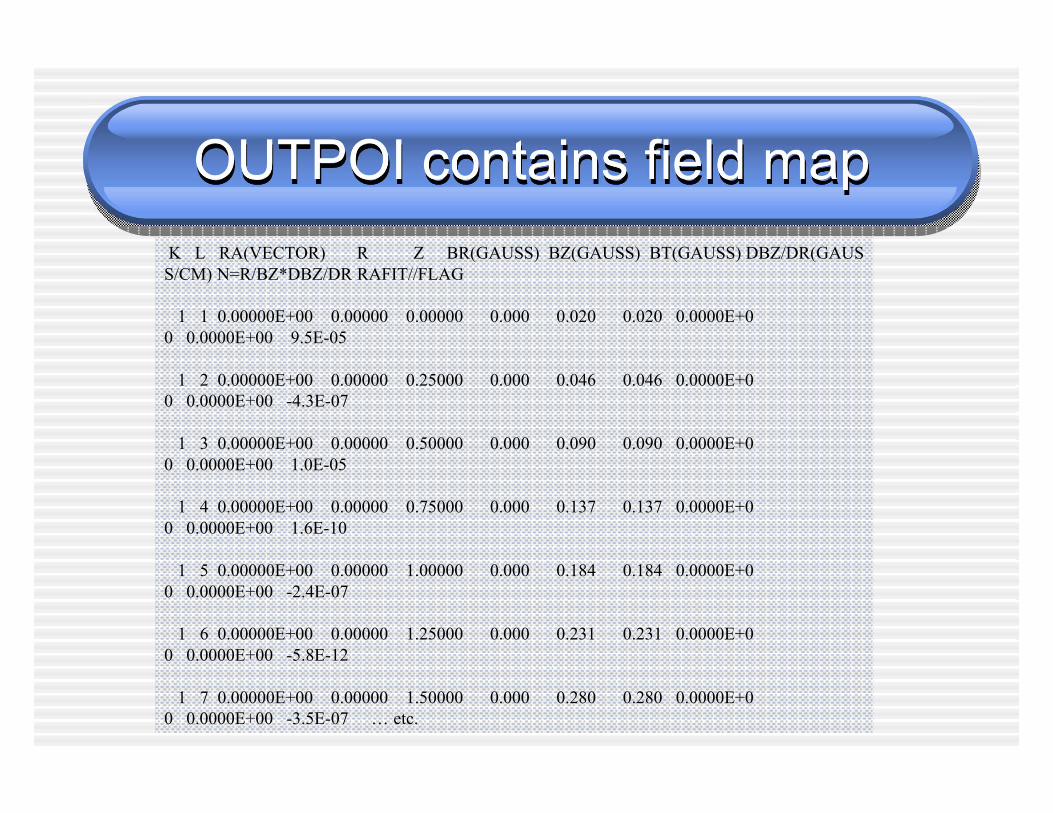
OUTPOI contains field mapOUTPOI contains field map

K L RA(VECTOR) R Z BR(GAUSS) BZ(GAUSS) BT(GAUSS) DBZ/DR(GAUS

S/CM) N=R/BZ*DBZ/DR RAFIT//FLAG

1 1 0.00000E+00 0.00000 0.00000 0.000 0.020 0.020 0.0000E+0

0 0.0000E+00 9.5E-05

1 2 0.00000E+00 0.00000 0.25000 0.000 0.046 0.046 0.0000E+0

0 0.0000E+00 -4.3E-07

1 3 0.00000E+00 0.00000 0.50000 0.000 0.090 0.090 0.0000E+0

0 0.0000E+00 1.0E-05

1 4 0.00000E+00 0.00000 0.75000 0.000 0.137 0.137 0.0000E+0

0 0.0000E+00 1.6E-10

1 5 0.00000E+00 0.00000 1.00000 0.000 0.184 0.184 0.0000E+0

0 0.0000E+00 -2.4E-07

1 6 0.00000E+00 0.00000 1.25000 0.000 0.231 0.231 0.0000E+0

0 0.0000E+00 -5.8E-12

1 7 0.00000E+00 0.00000 1.50000 0.000 0.280 0.280 0.0000E+0

0 0.0000E+00 -3.5E-07 … etc.

Reference:SPARC solenoidReference:SPARC solenoid

adjustable solenoid

$reg nreg=6,xmax=20.00,ymax=60.00,dx=0.25,dy=0.25,npoint=5$

$po x=0.000,y=0.000$

$po x=20.000,y=0.000$

$po x=20.000,y=60.000$

$po x=0.000,y=60.000$

$po x=0.000,y=0.000$


$po x=5.1,y=21.0$

$po x=16.8,y=21.0$

$po x=16.8,y=24.0$

$po x=5.1,y=24.0$

$po x=5.1,y=21.0$


$po x=5.1,y=25.0$

$po x=16.8,y=25.0$

$po x=16.8,y=28.0$

$po x=5.1,y=28.0$

$po x=5.1,y=25.0$


$po x=5.1,y=29.0$

$po x=16.8,y=29.0$

$po x=16.8,y=32.0$

$po x=5.1,y=32.0$

$po x=5.1,y=29.0$


$po x=5.1,y=33.0$

$po x=16.8,y=33.0$

$po x=16.8,y=36.0$

$po x=5.1,y=36.0$

$po x=5.1,y=33.0$


$po x=3.8,y=18.5$

$po x=19.3,y=18.5$

$po x=19.3,y=38.5$

$po x=3.8,y=38.5$

$po x=3.8,y=36.0$

$po x=16.8,y=36.0$

$po x=16.8,y=33.0$

$po x=4.5,y=33.0$

$po x=4.5,y=32.0$

$po x=16.8,y=32.0$

$po x=16.8,y=29.0$

$po x=4.5,y=29.0$

$po x=4.5,y=28.0$

$po x=16.8,y=28.0$

$po x=16.8,y=25.0$

$po x=4.5,y=25.0$

$po x=4.5,y=24.0$

$po x=16.8,y=24.0$

$po x=16.8,y=21.0$

$po x=3.8,y=21.0$

$po x=3.8,y=18.5$

Note four

current regions

Solenoid visual outputSolenoid visual output

• Translated relative to cathode

• Very little fringe field in gun region (to the right)…

Hybrid quad: Amperian currentsHybrid quad: Amperian currents

hybrid quad

$reg nreg=5, dx=0.1, xmax=15.0, ymax=15.0, xreg1=8.0, yreg1=8.0.,

npoint=5$

$po y= 0.00, x= 0.00$

$po y=15.00, x= 0.00$

$po y=15.00, x=15.00$

$po y= 0.00, x=15.00$

$po y= 0.00, x= 0.00$


$po x=0.000, y=10.795$

$po x=0.000, y=12.70$

$po x=3.393, y=12.70$

$po x=12.70, y=3.393$

$po x=12.70, y=0.00$

$po x=10.795, y=0.00$

$po x=10.795, y=2.604$

$po x=2.604, y=10.795$

$po x=0.000, y=10.795$


$po x=1.087, y=6.026$

$po x=6.026, y=1.087$

$po x=5.397, y=0.458$

$po x=.118, y=.588, x0=4.901, y0=.121, nt=2$

$po y=5.019, x=.709, r=2.668 nt=3$

$po x=0.337, y=.496, x0=0.121, y0=4.901, nt=2$

$po x=1.087, y=6.026$

$reg mat=1, cur=-28300., npoint=5$

$po x=4.521, y=8.877$

$po x=4.621, y=8.777$

$po x=1.479, y=5.634$

$po x=1.379, y=5.734$

$po x=4.521, y=8.877$

$reg mat=1, cur=28300., npoint=5$

$po y=4.521, x=8.877$

$po y=4.621, x=8.777$

$po y=1.479, x=5.634$

$po y=1.379, x=5.734$

$po y=4.521, x=8.877$

Very narrow

Current regions

(sheets)

Not always stable

K = M /µ0

Hybrid quad outputHybrid quad output

• Finite width Amperian current“sheets”

• Not much fringing!

• Need 3D (RADIA)

• Can you scale this to smallsize?

Example: Halbach undulatorExample: Halbach undulator

• Done entirely with Amperian

currents (see input deck)

• Current sheets are zero

width (vert/horiz sheets

better…)

• Can you put iron around the

LCLS undulator?

Yes. Flux circulates entirely in

PM pieces and gap

• Also has serious 3D aspects

iron

One period of undulator

Documents

The POISSON and SUPERFIS H Suite H Suite - …pbpl.physics.ucla.edu/Education/Schools/USPAS_2004/SFISH...The POISSON and SUPERFISThe POISSON and SUPERFIS H Suite H Suite J.B. Rosenzweig