The point processes at turning points of large lozengetilings

Sevak Mkrtchyan

University of Rochester

Representation Theory, Mathematical Physics and Integrable SystemsJune 8, 2018

(parts joint with L. Petrov)

Lozenge tilings

Consider the triangular lattice.

Lozenge tilings

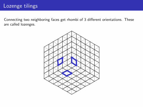
Connecting two neighboring faces get rhombi of 3 different orientations. Theseare called lozenges.

Lozenge tilings

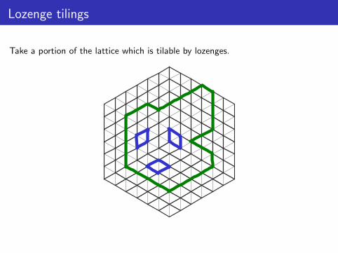
Take a portion of the lattice which is tilable by lozenges.

Lozenge tilings

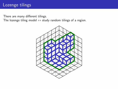
There are many different tilings.The lozenge tiling model ↔ study random tilings of a region.

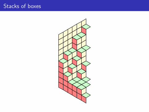
Stacks of boxes

Lattice paths

Limit shapes

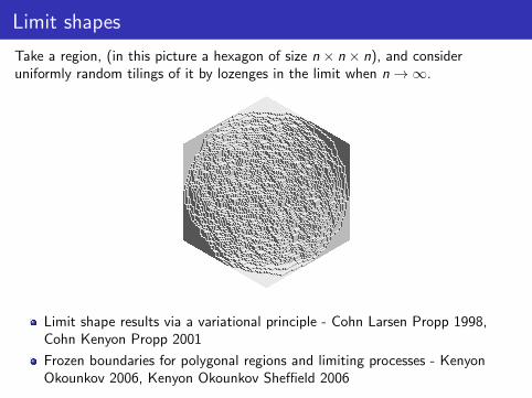
Take a region, (in this picture a hexagon of size n × n × n), and consideruniformly random tilings of it by lozenges in the limit when n→∞.

Limit shape results via a variational principle - Cohn Larsen Propp 1998,Cohn Kenyon Propp 2001

Frozen boundaries for polygonal regions and limiting processes - KenyonOkounkov 2006, Kenyon Okounkov Sheffield 2006

Infinite regions - volume measure

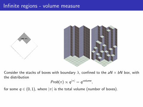
Consider the stacks of boxes with boundary λ, confined to the aN × bN box, withthe distribution

Prob(π) ∝ q|π| = qvolume ,

for some q ∈ (0, 1), where |π| is the total volume (number of boxes).

Limit shapes - infinite regions

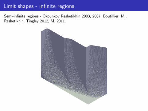
Semi-infinite regions - Okounkov Reshetikhin 2003, 2007, Boutillier, M.,Reshetikhin, Tingley 2012, M. 2011.

Scaling limit - limit shape

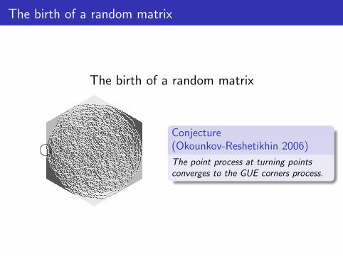
The birth of a random matrix

The birth of a random matrix

Conjecture(Okounkov-Reshetikhin 2006)

The point process at turning pointsconverges to the GUE corners process.

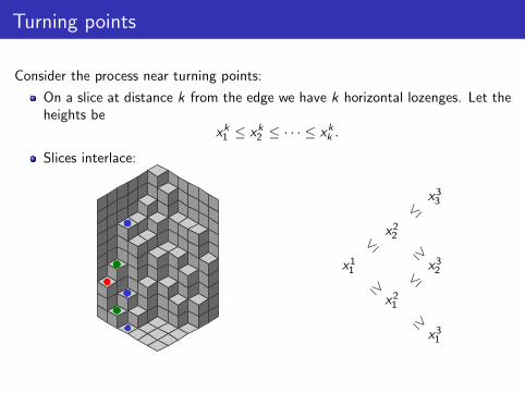
Turning points

Consider the process near turning points:

On a slice at distance k from the edge we have k horizontal lozenges. Let theheights be

xk1 ≤ xk2 ≤ · · · ≤ xkk .

Slices interlace:

x33

≤x2

2

≤ ≥x1

1 x32

≥ ≤x2

1

≥x3

1

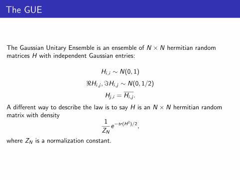
The GUE

The Gaussian Unitary Ensemble is an ensemble of N × N hermitian randommatrices H with independent Gaussian entries:

Hi,i ∼ N(0, 1)

<Hi,j ,=Hi,j ∼ N(0, 1/2)

Hj,i = Hi,j .

A different way to describe the law is to say H is an N × N hermitian randommatrix with density

1

ZNe−tr(H2)/2,

where ZN is a normalization constant.

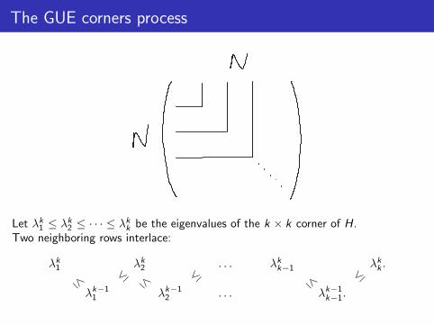
The GUE corners process

Let λk1 ≤ λk2 ≤ · · · ≤ λkk be the eigenvalues of the k × k corner of H.Two neighboring rows interlace:

λk1 λk2 . . . λkk−1 λkk .≤ ≤ ≤ ≤ ≤ ≤λk−1

1 λk−12 . . . λk−1

k−1.

The GUE corners process

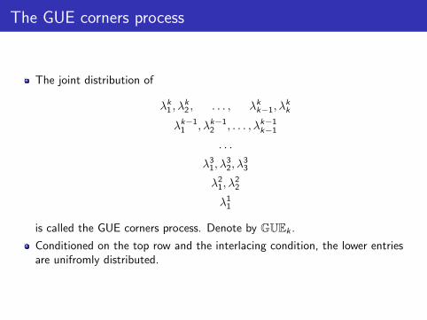
The joint distribution of

λk1 , λk2 , . . . , λkk−1, λ

kk

λk−11 , λk−1

2 , . . . , λk−1k−1

. . .

λ31, λ

32, λ

33

λ21, λ

22

λ11

is called the GUE corners process. Denote by GUEk .

Conditioned on the top row and the interlacing condition, the lower entriesare unifromly distributed.

The Okounkov-Reshetikhin conjecture

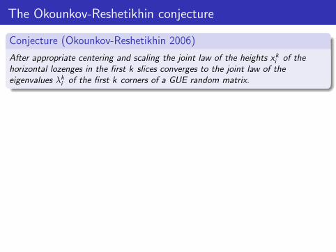
Conjecture (Okounkov-Reshetikhin 2006)

After appropriate centering and scaling the joint law of the heights xki of thehorizontal lozenges in the first k slices converges to the joint law of theeigenvalues λki of the first k corners of a GUE random matrix.

Prob(π) ∝ q|π| = qvolume

q ∈ (0, 1)

Let xki , i ≤ k be the heights ofthe first k slices as defined

above.

Theorem (Okounkov-Reshetikhin 2006)

Let q = e−1/N . There exist constants C0 and C1 such that in the limit q → 1 we

havexki −NC0√NC1

→ GUEk in distribution.

The Okounkov-Reshetikhin conjecture

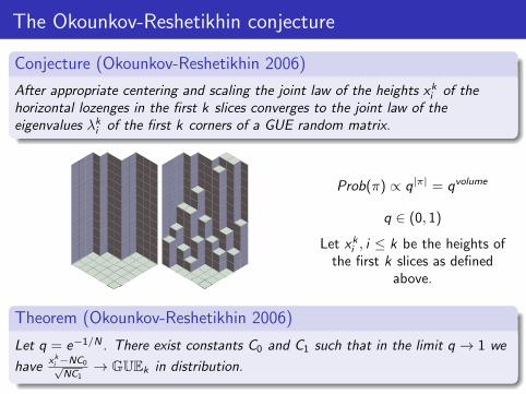
Conjecture (Okounkov-Reshetikhin 2006)

After appropriate centering and scaling the joint law of the heights xki of thehorizontal lozenges in the first k slices converges to the joint law of theeigenvalues λki of the first k corners of a GUE random matrix.

Prob(π) ∝ q|π| = qvolume

q ∈ (0, 1)

Let xki , i ≤ k be the heights ofthe first k slices as defined

above.

Theorem (Okounkov-Reshetikhin 2006)

Let q = e−1/N . There exist constants C0 and C1 such that in the limit q → 1 we

havexki −NC0√NC1

→ GUEk in distribution.

CLT for the turning point

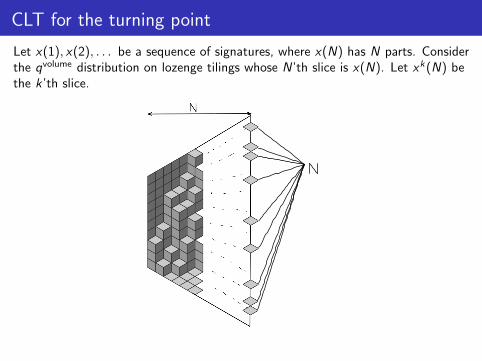
Let x(1), x(2), . . . be a sequence of signatures, where x(N) has N parts. Considerthe qvolume distribution on lozenge tilings whose N’th slice is x(N). Let xk(N) bethe k’th slice.

CLT for the turning point

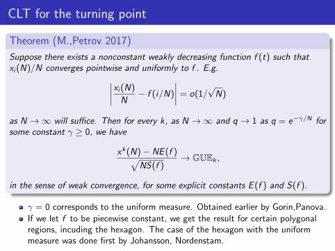
Theorem (M.,Petrov 2017)

Suppose there exists a nonconstant weakly decreasing function f (t) such thatxi (N)/N converges pointwise and uniformly to f . E.g.∣∣∣∣xi (N)

N− f (i/N)

∣∣∣∣ = o(1/√N)

as N →∞ will suffice. Then for every k , as N →∞ and q → 1 as q = e−γ/N forsome constant γ ≥ 0, we have

xk(N)− NE (f )√NS(f )

→ GUEk ,

in the sense of weak convergence, for some explicit constants E (f ) and S(f ).

γ = 0 corresponds to the uniform measure. Obtained earlier by Gorin,Panova.If we let f to be piecewise constant, we get the result for certain polygonalregions, incuding the hexagon. The case of the hexagon with the uniformmeasure was done first by Johansson, Nordenstam.

Breaking away from the GUE corners process

Given {qi}i∈Z, qi > 0, consider plane partitions with the distribution

Prob(π) ∝∏i∈Z

q|πi |i ,

where |πi | is the total volume of the i-th slice of π.

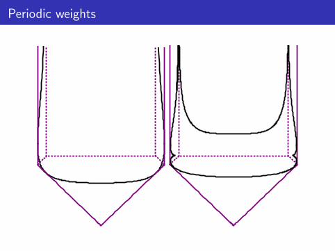
Periodic weights

Consider weights with

q0 = q±k = q±2k = . . .

q1 = q±k+1 = q±2k+1 = . . .

q2 = q±k+2 = q±2k+2 = . . .

. . .

qk−1 = q±2k−1 = q±3k−1 = . . .

What scaling limit should we study?

For simplicity, set k = 2 for now.

Nothing new, if you take q0 → 1− and q1 → 1−.

More interesting: α ≥ 1, q0 = αq, q1 = α−1q and q → 1−.

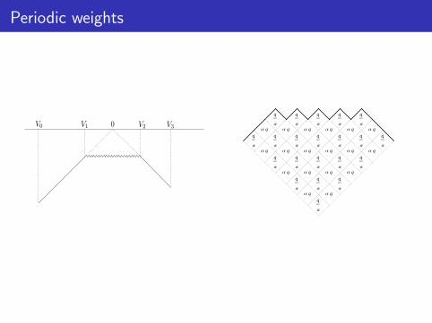
Periodic weights

q

Α

Α q

q

Α

Α q

q

Α

Α q

q

Α

Α q

q

Α

Α q

q

Α

Α q

q

Α

Α q

q

Α

Α q

q

Α

Α q

q

Α

Α q

q

Α

Α q

q

Α

Α q

q

Α

Α q

q

Α

q

Α

Α q

q

Α

Α q

q

Α

Α q

q

Α

Α q

q

Α

q

Α

Α q

q

Α

Periodic weights

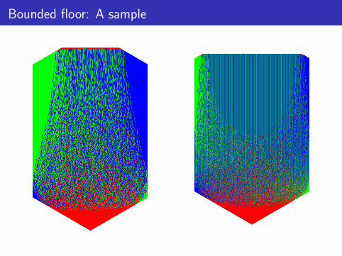
Bounded floor: A sample

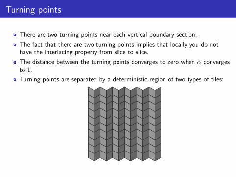
Turning points

There are two turning points near each vertical boundary section.

The fact that there are two turning points implies that locally you do nothave the interlacing property from slice to slice.

The distance between the turning points converges to zero when α convergesto 1.

Turning points are separated by a deterministic region of two types of tiles:

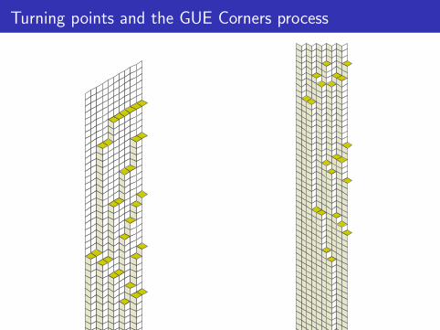
Turning points and the GUE Corners process

Turning point correlations

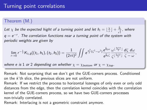
Theorem (M.)

Let χ be the expected hight of a turning point and let hi = bχr c+ h̃i

r12

, where

q = e−r . The correlation functions near a turning point of the system withperiodic weights are given by

limr→0

r−12 Kλ,q̄((t1, h1), (t2, h2)) =

1

(2πi)2

∫∫eσ2

2 (ζ2−ω2) eh̃2ω

e h̃1ζ

ωbt2+e

2 c

ζbt1+e

2 c

dζ dω

ζ − ω,

where e is 1 or 2 depending on whether χ = χbottom or χ = χtop.

Remark: Not surprising that we don’t get the GUE-corners process. Conditionedon the k’th slice, the previous slices are not uniform.Remark: If we restrict the process to horizontal lozenges of only even or only odddistances from the edge, then the correlation kernel coincides with the correlationkernel of the GUE-corners process, so we have two GUE-corners processesnon-trivially correlated.Remark: Interlacing is not a geometric constraint anymore.

General k

What happens for arbitrary finite period k for the weights?

Consider weightsqi = αiq,

i = 1, . . . , k , with qj = qj+k ,∀j . Let

k∏i=1

αi = 1

and consider the limit q → 1−.

If we have αi > 1 for some i , we run into the same issues with the measurebeing infinite as before.

Modifying the boundary as in the case k = 2 does not work anymore.

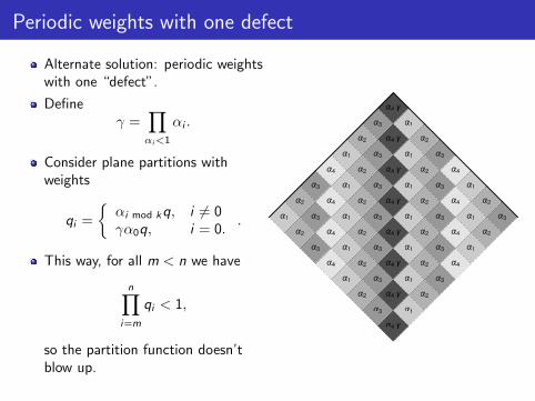
Periodic weights with one defect

Alternate solution: periodic weightswith one “defect”.

Defineγ =

∏αi<1

αi .

Consider plane partitions withweights

qi =

{αi mod kq, i 6= 0γα0q, i = 0.

.

This way, for all m < n we have

n∏i=m

qi < 1,

so the partition function doesn’tblow up.

α4 γ

α3

α2

α1

α4

α3

α2

α1

α1

α4 γ

α3

α2

α1

α4

α3

α2

α2

α1

α4 γ

α3

α2

α1

α4

α3

α3

α2

α1

α4 γ

α3

α2

α1

α4

α4

α3

α2

α1

α4 γ

α3

α2

α1

α1

α4

α3

α2

α1

α4 γ

α3

α2

α2

α1

α4

α3

α2

α1

α4 γ

α3

α3

α2

α1

α4

α3

α2

α1

α4 γ

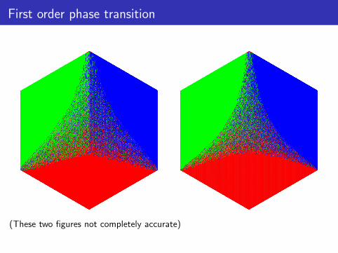
First order phase transition

(These two figures not completely accurate)

Turning points with k-periodic weights

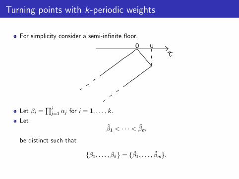
For simplicity consider a semi-infinite floor.

0 u

Let βi =∏i

j=1 αj for i = 1, . . . , k .

Letβ̃1 < · · · < β̃m

be distinct such that

{β1, . . . , βk} = {β̃1, . . . , β̃m}.

Turning points for k-periodic weights

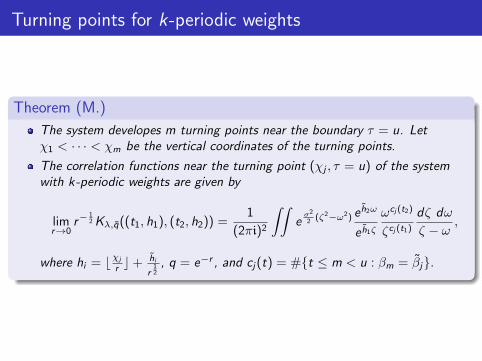
Theorem (M.)

The system developes m turning points near the boundary τ = u. Letχ1 < · · · < χm be the vertical coordinates of the turning points.

The correlation functions near the turning point (χj , τ = u) of the systemwith k-periodic weights are given by

limr→0

r−12 Kλ,q̄((t1, h1), (t2, h2)) =

1

(2πi)2

∫∫eσ2

2 (ζ2−ω2) eh̃2ω

e h̃1ζ

ωcj (t2)

ζcj (t1)

dζ dω

ζ − ω,

where hi = bχj

r c+ h̃i

r12

, q = e−r , and cj(t) = #{t ≤ m < u : βm = β̃j}.

GUE corners, Semi-frozen regions

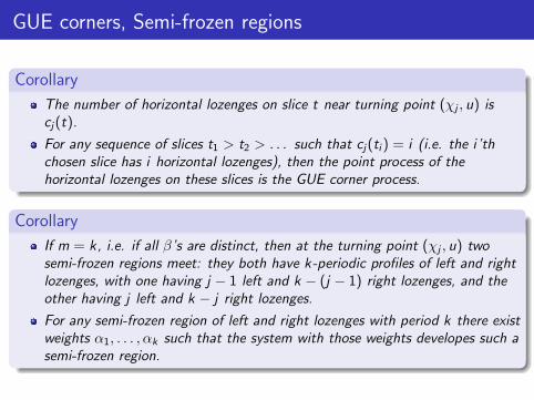
Corollary

The number of horizontal lozenges on slice t near turning point (χj , u) iscj(t).

For any sequence of slices t1 > t2 > . . . such that cj(ti ) = i (i.e. the i ’thchosen slice has i horizontal lozenges), then the point process of thehorizontal lozenges on these slices is the GUE corner process.

Corollary

If m = k, i.e. if all β’s are distinct, then at the turning point (χj , u) twosemi-frozen regions meet: they both have k-periodic profiles of left and rightlozenges, with one having j − 1 left and k − (j − 1) right lozenges, and theother having j left and k − j right lozenges.

For any semi-frozen region of left and right lozenges with period k there existweights α1, . . . , αk such that the system with those weights developes such asemi-frozen region.

Intermediate regime

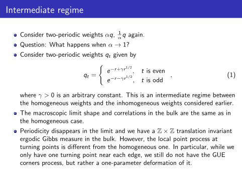
Consider two-periodic weights αq, 1αq again.

Question: What happens when α→ 1?

Consider two-periodic weights qt given by

qt =

{e−r+γr1/2

, t is even

e−r−γr1/2

, t is odd, (1)

where γ > 0 is an arbitrary constant. This is an intermediate regime betweenthe homogeneous weights and the inhomogeneous weights considered earlier.

The macroscopic limit shape and correlations in the bulk are the same as inthe homogeneous case.

Periodicity disappears in the limit and we have a Z× Z translation invariantergodic Gibbs measure in the bulk. However, the local point process atturning points is different from the homogeneous one. In particular, while weonly have one turning point near each edge, we still do not have the GUEcorners process, but rather a one-parameter deformation of it.

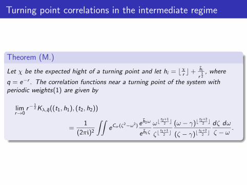
Turning point correlations in the intermediate regime

Theorem (M.)

Let χ be the expected hight of a turning point and let hi = bχr c+ h̃i

r12

, where

q = e−r . The correlation functions near a turning point of the system withperiodic weights(1) are given by

limr→0

r−12 Kλ,q̄((t1, h1), (t2, h2))

=1

(2πi)2

∫∫eCcr (ζ2−ω2) e

h̃2ω

e h̃1ζ

ωbt2+1

2 c

ζbt1+1

2 c

(ω − γ)bt2+2

2 c

(ζ − γ)bt1+2

2 c

dζ dω

ζ − ω.

Happy Birthday