The Phase-Space Approach to LFVThe Phase-Space Approach to LFV: Particles and Waves, Model Hierarchies and Data Sets

The Phase-Space Approach to LFVThe Phase-Space Approach to LFV: Particles and Waves, Model Hierarchies and Data Sets

Michael GhilEcole Normale Supérieure, Paris, and University of California, Los Angeles

Joint work with many people, most recently:

R. Berk, U. Penn.; F. D’Andrea, LMD/ENS, Paris; A. Deloncle, Ecole Polytechnique, Paris; B. Deremble, ENS, Paris; D. Kondrashov, UCLA

Pls. see this site for further details: http://www.atmos.ucla.edu/tcd/,

MotivationMotivation• The atmosphere is an open system subject to multiple

instabilities that interact nonlinearly and are limited in energy.• Bounded energy and prevalence of dissipation suggest the existence of

lower-dimensional attractors; instabilities and observations suggest that these are strange or worse.

• Boundedness in phase space and observations also suggest recurrence of large-scale features on time scales of interest.

• Two types of recurrent, but unstable features — fixed points (“particles”) and limit cycles (“waves”) — seem to dominatelow-frequency variability (LFV).

• They lie at the basis of two approaches to long-range forecasting (LRF): Markov chains and spectral methods.

• Simple, “toy” models can provide useful ideas, while thehierarchical modeling approach allows one to goback-and-forth between toy (“conceptual”) and detailed (“realistic”) models, and between models and data.

• The atmosphere is an open system subject to multipleinstabilities that interact nonlinearly and are limited in energy.

• Bounded energy and prevalence of dissipation suggest the existence of lower-dimensional attractors; instabilities and observations suggest that these are strange or worse.

• Boundedness in phase space and observations also suggest recurrence of large-scale features on time scales of interest.

• Two types of recurrent, but unstable features — fixed points (“particles”) and limit cycles (“waves”) — seem to dominatelow-frequency variability (LFV).

• They lie at the basis of two approaches to long-range forecasting (LRF): Markov chains and spectral methods.

• Simple, “toy” models can provide useful ideas, while thehierarchical modeling approach allows one to goback-and-forth between toy (“conceptual”) and detailed (“realistic”) models, and between models and data.

LFV* Observations:LFV* Observations:Multiple space and time scalesMultiple space and time scales

LFV* Observations:LFV* Observations:Multiple space and time scalesMultiple space and time scales

A high-variability

ridge lies close to the diagonal of the plot

(cf. also Fraedrich &

Böttger, 1978, JAS)

* LFVLFV 10–100 days (intraseasonal)

A high-variability

ridge lies close to the diagonal of the plot

(cf. also Fraedrich &

Böttger, 1978, JAS)

* LFVLFV 10–100 days (intraseasonal)

Blocking: a paradigm of persistent anomalyBlocking: a paradigm of persistent anomalyBlocking: a paradigm of persistent anomalyBlocking: a paradigm of persistent anomaly

Bauer, Namias, Rex and

many others noticed the

recurrence and

persistence of blocking.

J. Charney decided to go

beyond “talking about it,”

and actually “do

something about it.”

Bauer, Namias, Rex and

many others noticed the

recurrence and

persistence of blocking.

J. Charney decided to go

beyond “talking about it,”

and actually “do

something about it.”

QuickTime™ et undécompresseur TIFF (non compressé)

sont requis pour visionner cette image.

Monthly mean 500-hPa map

for January 1963 (from

Ghil & Childress, 1987)

Transitions Between Blocked and Zonal Flows

in a Rotating Annulus with Topography

Transitions Between Blocked and Zonal Flows

in a Rotating Annulus with Topography

Zonal Flow Blocked Flow 13–22 Dec. 1978 10–19 Jan. 1963

E.R. Weeks, Y. Tian, J. S. Urbach, K. Ide, H. L. Swinney, & M. Ghil, 1997: Science, 278, 1598–1601.

A toy model for blocking vs. zonal flow

A toy model for blocking vs. zonal flow Quasi-geostrophic flow in a

mid-latitude -channel,

with 3-mode truncation

(zonal + 1 wave). Topographic resonance

leads to multiple

equilibria: zonal + blocked. Much criticized as

“unrealistic.”

Quasi-geostrophic flow in a

mid-latitude -channel,

with 3-mode truncation

(zonal + 1 wave). Topographic resonance

leads to multiple

equilibria: zonal + blocked. Much criticized as

“unrealistic.”

Charney & DeVore, 1979:

J. Atmos. Sci., 36, 1205–1216.

From RegimesFrom Regimes to Markov ChainsFrom RegimesFrom Regimes to Markov Chains

Each regime R has an expected duration R.

Expected transition probability from regime

A to B is pAB. Transitions do NOT occur

via the mean state, which is a statistical “accident” or, maybe, the root of the “bifurcation tree.”

Each regime R has an expected duration R.

Expected transition probability from regime

A to B is pAB. Transitions do NOT occur

via the mean state, which is a statistical “accident” or, maybe, the root of the “bifurcation tree.”

From Ghil (1987), in

Nicolis & Nicolis (eds.).

How to get from a regime How to get from a regime to another? – Ito another? – I

How to get from a regime How to get from a regime to another? – Ito another? – I

Stochastic perturbations

Heteroclinic and

homoclinic orbits Chaotic itinerancy All of the above

Stochastic perturbations

Heteroclinic and

homoclinic orbits Chaotic itinerancy All of the above

Ghil & Childress, 1987: Ch. 6

Multiple Flow RegimesMultiple Flow RegimesMultiple Flow RegimesMultiple Flow RegimesA. Classification schemes1) By position (i) Cluster analysis– categorical – NH, Mo & Ghil (1988, JGR) – fuzzy

– NH + sectorial, Michelangeli et al. (1995, JAS) – hard (K–means) – hierarchical – NH + sectorial, Cheng & Wallace (1993, JAS)

(ii) PDF estimation – univariate: – NH, Benzi et al. (1986, QJRMS); Hansen & Sutera (1995, JAS)– multivariate:– NH, Molteni et al. (1990, QJRMS); Kimoto & Ghil (1993a, JAS– sectorial, Kimoto & Ghil (1993b, JAS); Smyth et al. (1999, JAS)

2) By persistence (iii) Pattern correlations

– NH, Horel (1985, MWR); SH, Mo & Ghil (1987, JAS) (iv) Minima of tendencies

– Models: Legras & Ghil (1985, JAS); Mukougawa (1988, JAS); Vautard & Legras (1988, JAS)

– Atl.- Eur. sector : Vautard (1990, MWR)B. Transition probabilities

(v) Model & NH – counts (Mo & Ghil, 1988, JGR)(vi) NH & SH – Monte Carlo (Vautard et al., 1990, JAS)

A. Classification schemes1) By position (i) Cluster analysis– categorical – NH, Mo & Ghil (1988, JGR) – fuzzy

– NH + sectorial, Michelangeli et al. (1995, JAS) – hard (K–means) – hierarchical – NH + sectorial, Cheng & Wallace (1993, JAS)

(ii) PDF estimation – univariate: – NH, Benzi et al. (1986, QJRMS); Hansen & Sutera (1995, JAS)– multivariate:– NH, Molteni et al. (1990, QJRMS); Kimoto & Ghil (1993a, JAS– sectorial, Kimoto & Ghil (1993b, JAS); Smyth et al. (1999, JAS)

2) By persistence (iii) Pattern correlations

– NH, Horel (1985, MWR); SH, Mo & Ghil (1987, JAS) (iv) Minima of tendencies

– Models: Legras & Ghil (1985, JAS); Mukougawa (1988, JAS); Vautard & Legras (1988, JAS)

– Atl.- Eur. sector : Vautard (1990, MWR)B. Transition probabilities

(v) Model & NH – counts (Mo & Ghil, 1988, JGR)(vi) NH & SH – Monte Carlo (Vautard et al., 1990, JAS)

How to get from a regime How to get from a regime to another? – IIto another? – II

How to get from a regime How to get from a regime to another? – IIto another? – II

Even something as simple as a periodically forced damped pendulum can have complex behavior.

Here are 4 attractor basins, each with a different type of

behavior. Time to get there is shown by

brightness of color.

Even something as simple as a periodically forced damped pendulum can have complex behavior.

Here are 4 attractor basins, each with a different type of

behavior. Time to get there is shown by

brightness of color.

QuickTime™ et undécompresseur TIFF (non compressé)

sont requis pour visionner cette image.

http://www-chaos.umd.edu/gallery/basinpics.html

Preferred Transition PathsPreferred Transition PathsPreferred Transition PathsPreferred Transition Paths Conjectured by Legras & Ghil (JAS, 1985) in toy model (25 Yn

m). Captured by Kondrashov et al. (JAS, 2004) in intermediate QG3 (Marshall & Molteni,

1993) model. Exit angles used as predictors in statistical, random-forests algorithm:

Conjectured by Legras & Ghil (JAS, 1985) in toy model (25 Ynm).

Captured by Kondrashov et al. (JAS, 2004) in intermediate QG3 (Marshall & Molteni, 1993) model.

Exit angles used as predictors in statistical, random-forests algorithm:

- for QG3 model by

Deloncle et al. (JAS, 2006);

- for NH reanalysis data by

Kondrashov et al.

(Clim. Dyn., 2007).

NWP Model Performance on BlockingNWP Model Performance on BlockingNWP Model Performance on BlockingNWP Model Performance on Blocking

Leading numerical

weather prediction (NWP)

models still underestimate

badly blocking occurrence

and persistence:ECMWF - European Centre

Met Office - United Kingdom

CNRM - Météo-France

Leading numerical

weather prediction (NWP)

models still underestimate

badly blocking occurrence

and persistence:ECMWF - European Centre

Met Office - United Kingdom

CNRM - Météo-France

ECMWF

CNRM

Met Office

Era40

model

T. N. Palmer et al., 2007:

Bull. Amer. Met. Soc.,

sub judice (pers. commun.)

A few questionsleft:A few questionsleft: Are the regimes but slow phases

of the oscillations? Are the oscillations but

instabilities of particularfixed points?

How about both?– chaotic itinerancy

How about neither?– just interference of linear waves;– just red noise.

Are the regimes but slow phases of the oscillations?

Are the oscillations but instabilities of particularfixed points?

How about both?– chaotic itinerancy

How about neither?– just interference of linear waves;– just red noise.

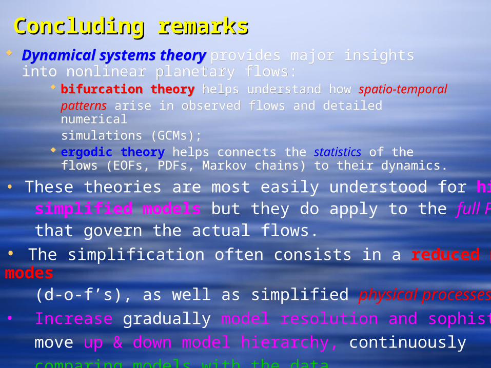
Concluding remarksConcluding remarksConcluding remarksConcluding remarks Dynamical systems theory provides major insights into

nonlinear planetary flows: bifurcation theory helps understand how spatio-temporal

patterns arise in observed flows and detailed numerical simulations (GCMs);

ergodic theory helps connects the statistics of the flows (EOFs, PDFs, Markov chains) to their dynamics.

Dynamical systems theory provides major insights into nonlinear planetary flows:

bifurcation theory helps understand how spatio-temporal patterns arise in observed flows and detailed numerical simulations (GCMs);

ergodic theory helps connects the statistics of the flows (EOFs, PDFs, Markov chains) to their dynamics.

• These theories are most easily understood for highly simplified models but they do apply to the full PDE systems that govern the actual flows.

• The simplification often consists in a reduced number of modes (d-o-f’s), as well as simplified physical processes.

• Increase gradually model resolution and sophistication:

move up & down model hierarchy, continuously

comparing models with the data.

Some general referencesSome general referencesLorenz, E. N., 1963b: The mechanics of vacillation. J. Atmos. Sci., 20, 448–464.Charney, J.G., and J. DeVore, 1979: Multiple flow equilibria in the atmosphere and

blocking. J. Atmos. Sci., 36, 1205–1216. Charney, J. G., J. Shukla, and K. C. Mo, 1981: Comparison of a barotropic blocking

theory with observation. J. Atmos. Sci., 38, 762–779. Charney, J. G. and D. M. Straus, 1981: Form-drag instability, multiple equilibria and

propagating planetary waves in baroclinic, orographically forced planetary wave systems. J. Atmos. Sci., 38, 1157–1176.

Ghil, M., R. Benzi, and G. Parisi (Eds.), 1985: Turbulence and Predictability in Geophysical Fluid Dynamics and Climate Dynamics, North-Holland, 449 pp.

Ghil, M., and S. Childress, 1987: Topics in Geophysical Fluid Dynamics: Atmospheric Dynamics, Dynamo Theory and Climate Dynamics, Springer-Verlag, 485 pp.

Corti, S., F. Molteni, and T. N. Palmer, 1999 "Signature of recent climate change in frequencies of natural atmospheric circulation regimes". Nature, 398, 799–802.

Ghil, M., and A. W. Robertson, 2002: "Waves" vs. "particles" in the atmosphere's phase space: A pathway to long-range forecasting? Proc. Natl. Acad. Sci. USA, 99(Suppl. 1), 2493–2500.

Kalnay, E., 2003. Atmospheric Modeling, Data Assimilation and Predictability.Cambridge Univ. Press, Cambridge/London, 341 pp.

Ghil, M., and E. Simonnet, 2007: Nonlinear Climate Theory, Cambridge Univ. Press, Cambridge, UK/London/New York, in preparation (approx. 450 pp.).

Lorenz, E. N., 1963b: The mechanics of vacillation. J. Atmos. Sci., 20, 448–464.Charney, J.G., and J. DeVore, 1979: Multiple flow equilibria in the atmosphere and

blocking. J. Atmos. Sci., 36, 1205–1216. Charney, J. G., J. Shukla, and K. C. Mo, 1981: Comparison of a barotropic blocking

theory with observation. J. Atmos. Sci., 38, 762–779. Charney, J. G. and D. M. Straus, 1981: Form-drag instability, multiple equilibria and

propagating planetary waves in baroclinic, orographically forced planetary wave systems. J. Atmos. Sci., 38, 1157–1176.

Ghil, M., R. Benzi, and G. Parisi (Eds.), 1985: Turbulence and Predictability in Geophysical Fluid Dynamics and Climate Dynamics, North-Holland, 449 pp.

Ghil, M., and S. Childress, 1987: Topics in Geophysical Fluid Dynamics: Atmospheric Dynamics, Dynamo Theory and Climate Dynamics, Springer-Verlag, 485 pp.

Corti, S., F. Molteni, and T. N. Palmer, 1999 "Signature of recent climate change in frequencies of natural atmospheric circulation regimes". Nature, 398, 799–802.

Ghil, M., and A. W. Robertson, 2002: "Waves" vs. "particles" in the atmosphere's phase space: A pathway to long-range forecasting? Proc. Natl. Acad. Sci. USA, 99(Suppl. 1), 2493–2500.

Kalnay, E., 2003. Atmospheric Modeling, Data Assimilation and Predictability.Cambridge Univ. Press, Cambridge/London, 341 pp.

Ghil, M., and E. Simonnet, 2007: Nonlinear Climate Theory, Cambridge Univ. Press, Cambridge, UK/London/New York, in preparation (approx. 450 pp.).