1

The Performance Persistence of Equity Long/Short Hedge Funds

Markus M. Schmida,# and Samuel Manserb

a Swiss Institute of Banking and Finance, University of St. Gallen, CH-9000 St. Gallen, Switzerland

b Credit Suisse Asset Management, CH-8000 Zurich, Switzerland

This version: 20 July 2008

Abstract

This paper examines persistence of raw and risk-adjusted returns for long/short equity hedge funds using the portfolio approach of Hendricks, Patel and Zeckhauser (1993). Only limited evidence of persistence is found for raw returns. Funds with the highest raw returns last year continue to outperform over the subsequent year, although not significantly while there is no persistence in returns beyond one year. In contrast, we find performance persis-tence based on risk-adjusted return measures such as the Sharpe Ratio and in particular an alpha from a multifactor model. Funds with the highest risk-adjusted performance continue to significantly outperform in the following year. The persistence does not last longer than one year except for the worst performers. Funds with significant risk-adjusted returns show less exposure to the market, have high raw returns and low volatility. These results are ro-bust to adjustments for stale prices and subperiod analysis.

Keywords: Performance persistence; Hedge funds; Equity long/short; Multifactor models JEL Classification: G11, G12 _______________________ # Contact address: Tel.: +41-71-224-70-31; fax: +41-71-224-70-88. E-mail: markus.schmid@unisg.ch. Address: Swiss Institute of Banking and Finance, University of St. Gallen, Rosenbergstrasse 52, CH-9000 St. Gallen, Switzerland.

2

Introduction

Studies examining the persistence of hedge fund performance vary a lot in their conclu-

sions due to different methodologies, databases, investigation periods, and performance

measures (e.g., Eling, 2007). This paper does not consider various approaches to clarify the

picture, but instead, focuses on a particularly flexible one. Every period, hedge funds are

sorted into portfolios according to characteristics in the last period and then the portfolios are

tracked for the next period. After the tracking period, the sorting is repeated. This approach

has been used in the mutual fund literature by Hendricks, Patel, and Zeckhauser (1993) and

Carhart (1997) among others and has several advantages. First, portfolio betas may be more

stable than betas of individual funds because time-varying betas can offset each other on the

portfolio level. This is particularly relevant for hedge funds: As they have fewer restrictions

on borrowing, shorting, the use of derivatives etc., they typically follow highly opportunistic

strategies that lead to time-varying risk exposures. Moreover, beta measurement is more pre-

cise due to diversification of idiosyncratic risk and long time series for the portfolio returns.

Finally, suppose there is only a very small autocorrelation in fund returns. Given the high re-

turn variance, it is difficult to detect this correlation by looking at individual funds. As in the

case of momentum strategies, we have to buy a portfolio of last period’s winners, not just one

fund, to see persistence.

This paper extends the current literature in several directions. First, by restricting the sam-

ple to long/short equity hedge funds, the number of (risk) factors can be greatly reduced while

the explanatory power of the factor models is maximized. In fact, the widely used factor mod-

els generally exhibit a very high explanatory power for the equity long/short strategy – in ab-

solute terms as well as relative to other strategies (e.g., Fung and Hsieh, 2002; Agarwal and

Naik, 2004; Fung and Hsieh, 2006). Given only monthly observations of hedge fund returns, a

low number of parameters is desirable as it renders inference more robust due to conservation

of degrees of freedom and mitigation of multicollinearity problems. Secondly and related,

3

prior studies generally pool different hedge fund strategies and analyze them jointly (e.g.,

Boyson and Cooper, 2004; Capocci, 2007). This can be susceptible to the problem of model

misspecification: Alpha portfolios may contain funds of the same strategy because neglected

risk factors for this strategy show up as alpha. Hence, results focusing on one particular strat-

egy may be more robust. Thirdly, possible nonlinear market exposure is accounted for by in-

cluding option returns as risk factors. Agarwal and Naik (2000, 2004) find that the systematic

risk exposure of hedge funds can include option-based strategies. However, no such exposure

has been found for long/short equity hedge funds on the aggregate level (Fung and Hsieh,

2006; Agarwal and Naik, 2004). Individual funds, on the other hand, may well show nonlin-

ear market exposure and it may be important to account for nonlinearities when evaluating

performance. Finally, we consider sorts based on regression coefficients. In order to examine

the nature of return persistence, it is important to know whether the momentum loading of

funds persists and whether these funds outperform.

The analysis in this paper is interesting for several reasons. First, repeatedly forming a

portfolio based on observable information and tracking it for the next period represents a trad-

ing strategy which is conceptually easily implementable. Practically, however, the typical

investor faces lockup periods prohibiting him from exploiting these strategies. Still, they may

be interesting for funds of funds that are able to waive lockup periods (Boyson and Cooper,

2004). Secondly, performance persistence may be more important for hedge funds than for

mutual funds due to their higher attrition rates (Capocci, Corhay, and Huebner, 2005). By

looking at funds’ transition probabilities of moving from one portfolio to another and by

tracking a portfolio not only one year but several years, one gets a clearer picture of the per-

sistence.

After a short overview of the literature, the factor model is introduced and applied on the

index level. Next, we present the dataset and sample selection procedures. The discussion of

the results is the main part and focuses on the persistence of raw returns as well as risk-

4

adjusted performance measures. In order to mitigate spurious results, various robustness tests

are performed before a conclusion is reached.

Literature overview

While the performance of mutual funds has been extensively studied in the academic lit-

erature, there is a growing body of literature on hedge fund performance persistence. Even

more than in the mutual fund literature, there is a large variance in the conclusions drawn by

the studies examining persistence of hedge fund performance. A recent overview of the litera-

ture on persistence of hedge fund performance is provided by Eling (2007). He shows that

these studies differ widely in methodology, database, investigation period, performance

measures and conclusions. To obtain a clearer picture, at a minimum, persistence of raw re-

turns and risk-adjusted returns have to be distinguished.

Harri and Brorsen (2004) report short-term persistence of three to four months with the

biggest effect in the first month based on simple regressions of returns on lagged returns.

Over the quarterly horizon (portfolios are reformed quarterly), Boyson and Cooper (2004)

obtain a monthly return spread of more than 1.14% using a pool of all hedge fund strategies.

For the annual horizon, Baquero, Jenke, and Verbeek (2004) find an insignificant spread of an

annual 4.9% and an annual spread of 11.5% at the quarterly horizon. Clearly, the smaller the

horizon the stronger the persistence in performance as measured by raw returns. Overall, the

literature is in favor of short-term persistence over horizons of up to six months but is mixed

with respect to annual persistence (Eling, 2007).

The evidence on the persistence of risk-adjusted performance is particularly mixed as

there are various methods and performance measures. Amenc, Curtis, and Martellini (2003)

show that different models strongly disagree on the risk-adjusted performance of hedge funds

because there is a large dispersion of alphas across models. Still, they generally tend to rank

the funds in a similar way. Common factor choices for hedge fund (risk) factors are the three

5

Fama-French factors, Carhart’s (1997) momentum factor, commodity, bond, and volatility

factors, factors representing returns to technical trading strategies such as the Fung and Hsieh

(2001) primitive trend-following factors1 or the Agarwal and Naik (2004) option-factors2.

Persistence can be examined using simple autoregressions, Spearman’s rank correlation, and

contingency tables as the most prominent methods. The evidence is mixed, however. For ex-

ample, while Agarwal and Naik (2000) find no persistence beyond the quarterly horizon,

Kosowski, Naik, and Teo (2005) and Edwards and Caglayan (2001) report annual persistence.

One prominent method introduced by Hendricks, Patel, and Zeckhauser (1993) and used

in the mutual fund literature (e.g., Carhart, 1997; Davis, 2001) consists of repeatedly forming

portfolios of funds based on lagged characteristics and tracking them for the next period. Boy-

son and Cooper (2004) sort on characteristics other than returns or alpha for hedge funds.

While they find no persistence when sorting on past performance alone, considering manager

tenure in addition leads to the finding of quarterly persistence. The persistence is mainly con-

centrated in the poor performers. However, considering all hedge fund strategies jointly, they

use up to 20 factors to end up with an R² of around 0.75. Capocci (2007) sorts portfolios

based on additional properties of the return distribution. He finds that portfolios of funds with

the highest lagged Sharpe Ratio deliver positive alpha. The same holds for funds with the

lowest volatility and, to a lesser extent, funds with low market beta. Sorting portfolios based

on higher moments of the return distribution or lagged alpha, however, does not detect a sig-

nificant alpha spread between top and bottom portfolios.

1 The factors are returns to primitive trend-following strategies of rolling over lookback-straddles on commodity, foreign exchange and bond futures. The owner of a lookback call (put) option has the right to buy (sell) the un-derlying at the lowest (highest) price over the life of the option. The combination of these is a lookback-straddle. 2 These factors are returns from rolling over call and puts of different moneyness with a broad market index as the underlying.

6

Model

Portfolio formation

The methodology to form portfolios is based on Hendricks, Patel, and Zeckhauser (1993).

On January 1st of each year, portfolios of hedge funds are formed based on specific character-

istics during the formation period and tracked for the subsequent year. Then, the portfolios are

reformed. The portfolios are numbered from 1 to 10, whereas portfolio 1 contains the 10% of

funds with, for example, the highest lagged returns and portfolio 10 contains the 10% of funds

with the lowest lagged returns. The weights of the funds in the portfolios are equal and read-

justed whenever a fund disappears during the tracking year. To provide additional informa-

tion, the deciles 1 and 10 are further subdivided into terciles, indicated by capital letters A, B

and C. Also, a portfolio which is long in portfolio 1 and short in portfolio 10 (long 1A and

short 10C) is analyzed.

In this paper, the tracking horizon is one year for two reasons. First, quarterly or even

monthly reforming of a portfolio would be difficult to implement as a trading strategy due to

lock-in periods. Secondly, because of illiquidity or managed prices, hedge fund managers

have leeway in marking their positions for month-end reporting. This flexibility can be used

to artificially reduce return volatility or market beta. The resulting returns spuriously show

short-term autocorrelation known as ‘stale prices’ (Asness, Krail, and Liew, 2001; Get-

mansky, Lo, and Marakov, 2004) which shows up as short-term persistence in returns. Fre-

quent portfolio reforming may therefore just take up this autocorrelation. Focusing on the

one-year horizon alleviates this problem. In the robustness section, we also explicitly control

for ‘stale prices’.

Factor benchmark and alpha

The first hedge fund was founded by Albert Winslow Jones in 1949 and involved simulta-

neous investments in long and short stock positions. Today, this strategy is being referred to

7

as 'long/short equity' as one particular style among others like global macro or merger arbi-

trage. Despite being a relatively old strategy, interest has remained strong. About 40% of all

funds provided by the CISDM database follow this strategy. A similar fraction holds for other

databases, e.g. TASS (Fung and Hsieh, 2004).

Long/short equity is a directional strategy which invests on both the long and short side of

the market. A long/short equity manager typically shorts stocks that he believes are overval-

ued and invests in more attractive stocks. Shorting stocks serves at least three purposes: It can

generate excess returns above a benchmark, hedge market (and other) risk and managers can

either use the proceeds of the short sale to finance the long positions or earn interest on them

(Fung and Hsieh, 2006). Equity long/short hedge funds generally exhibit a long-bias. How-

ever, the funds are by no means a homogenous group. Some managers attempt market neu-

trality while others choose a short bias. Moreover, they can vary their exposure over time.

Long/short equity funds shift from small to large caps, from growth to value, from momentum

to contrarian, and from long to short positions in stocks. Additionally, managers can use de-

rivatives and debt financing for leveraging. The focus can be regional, such as long/short U.S.

and European equity, or sector specific, such as long/short utilities and technology. According

to Asness, Krail, and Liew (2001), the holdings of these funds tend to be substantially more

concentrated than those of traditional stock funds. Summarizing, contrary to the buy-and-hold

approach of most mutual funds, hedge funds employ dynamic strategies in a wide range of

asset classes, use derivatives, and can be highly leveraged.

There are various reasons why hedge funds may show nonlinear market exposure: Hedge

funds are allowed to trade in derivatives and can employ option-like trading strategies. Agar-

wal and Naik (2004) find significant exposure of most hedge fund strategies to the return of

repeatedly buying and selling index options. Many strategies seem to behave like writing out-

of-the-money put options on the market index. As an example, suppose writing put options is

a profitable strategy over the time period considered. Then, the portfolio of past winners may

contain more put writers. As Glosten and Jagannathan (1994) show, such nonlinear payoffs

can outperform a linear benchmark. Hence, not including option factors could spuriously in-

dicate outperformance and neglect systematic (tail) risk.

The investment flexibility of hedge funds makes performance assessment more difficult.

Style-drift and exposure to a wide range of asset classes, possibly even nonlinear, must be

accounted for. Given the limited amount of data, this task can only be dealt with on a rudi-

mentary level. Possible nonlinearities are accounted for by including option-based strategies,

using a rolling-window approach, and performing an analysis of subperiods which may miti-

gate the effects of style-drift.

As hedge funds typically employ dynamic strategies, the static CAPM is an inappropriate

benchmark. For long/short equity funds, Fung and Hsieh (2006) show that the overall market

and the spread between large and small cap stocks account for over 80% of return variation on

the index level. Combined with a momentum factor, they find it unlikely to have omitted an

important risk factor. Hence, long/short equity returns can be well captured using the Fama-

French factors, a momentum factor and option factors to account for possible nonlinearities.

This can be represented with the following model that extends Carhart’s (1997) four-factor

model.

8

t, , , , , , ,

, i t f t i i RMRF t i SMB t i HML t i MOM t i OTMC

i OTMP t

R R RMRF SMB HML MOM OTMC

OTMP

α β β β β β

β

− = + + + + +

+

The left-hand side is the excess return of portfolio i in month t. RMRF is the excess return on

the market portfolio, proxied by the value-weighted return on all NYSE, AMEX, and

NASDAQ stocks minus the one-month Treasury bill rate. SMB is the excess return of the fac-

tor-mimicking portfolio for size, HML is the excess return of the factor-mimicking portfolio

for book-to-market equity, and MOM is the excess return of the factor-mimicking portfolio

for one-year momentum.3

Agarwal and Naik (2004) and Fung and Hsieh (2001) show that hedge funds can have ex-

posure to option returns on standard asset classes. Agarwal and Naik (2004) use returns of

rolling-over put and call options on the S&P 500. Here, a procedure very similar to Agarwal

and Naik (2004) is employed to obtain out-of-the-money (OTM) call and put option factors

on the S&P 500 index: On the first trading day in January, an OTM option on the S&P 500 is

bought that expires on the first trading day in February. On the first trading day in February

either the option is exercised or not. For a call option, for example, the return is calculated

using ⎟⎟⎠

⎞⎜⎜⎝

⎛−−

−= 1,1max

Jan

JanFebCall C

KSR where S is the value of the S&P 500 index, K the strike

price and C the call price in the respective months. Then, the same type of option maturing on

the first trading day in March is bought. For the OTM call (put) options, the strike price is 101

(99) percent of the S&P 500 at the time of purchase.4 Here, option prices are calculated using

the Black-Scholes formula for pricing European style options. Using historic volatility of the

underlying, it is known that Black-Scholes does not price options well that are deep in- or out-

of-the-money. As a compromise only OTM call and put factors are used with strike price of

101 (99) percent of the S&P 500 index value. This happens to be the ratio Agarwal and Naik

(2004) used for their out-of-the-money factors.5 By subtracting the riskfree rate from returns

of the rolling-over option strategy, one obtains the out-of-the-money call (OTMC) and out-of-

the-money put (OTMP) factors.

3 These factors are provided by Kenneth French on http://mba.tuck.dartmouth.edu/pages/faculty/ken.french. 4 Agarwal and Naik (2004) use market prices but their data is currently only available until January 2005.

9

5 Agarwal and Naik (2004) also use at-the-money option factors. Due to the high correlation of option factors of similar moneyness, these are left out. Besides, especially the OTM put factor has been significant in Agarwal and Naik (2004). The correlation of their series and the one used here is around 0.85 for both OTM put and call options. The volatility of the underlying is estimated using the realized standard deviation of the S&P 500 index during the preceding month. Data on the S&P 500 and the dividend yield was obtained from Datastream and the risk free rate from Kenneth French’s Data Library.

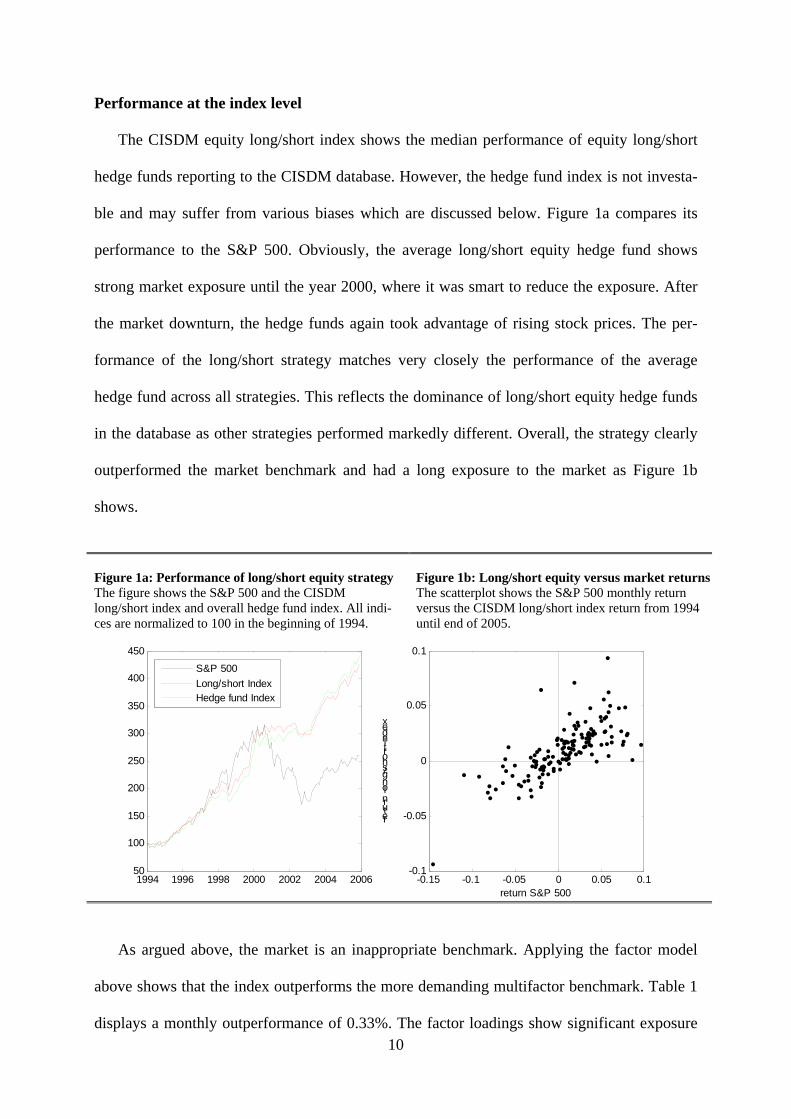
Performance at the index level

The CISDM equity long/short index shows the median performance of equity long/short

hedge funds reporting to the CISDM database. However, the hedge fund index is not investa-

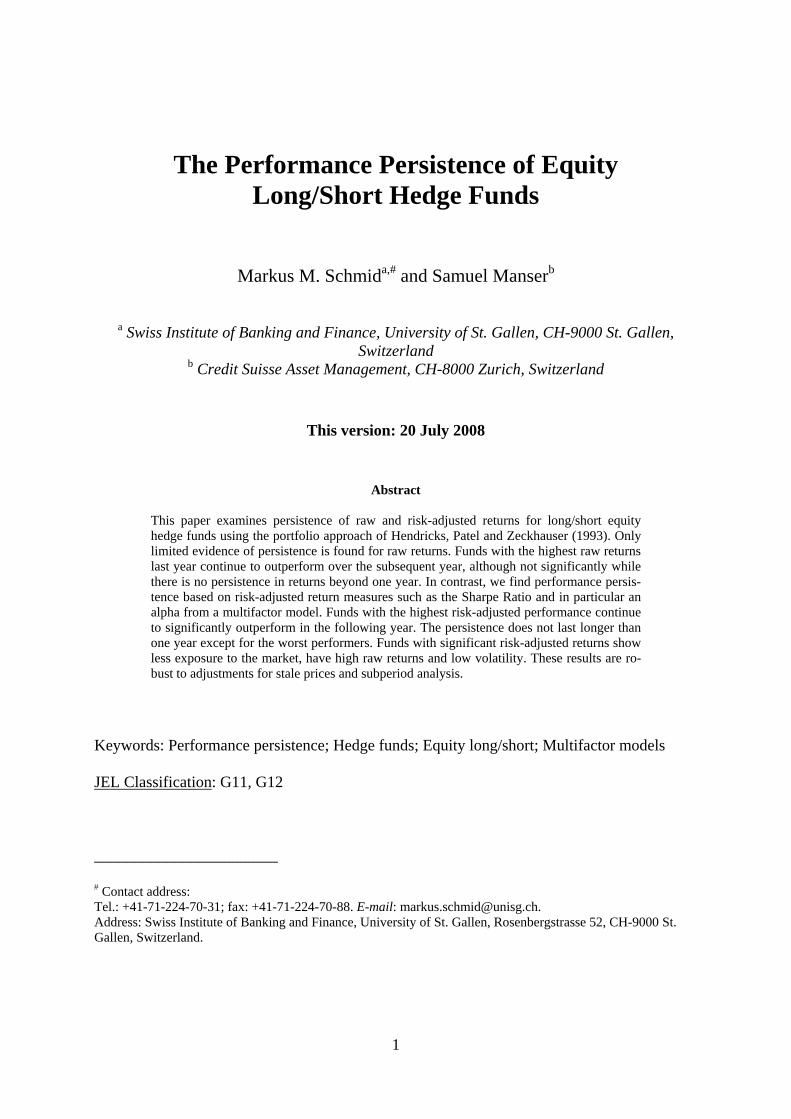
ble and may suffer from various biases which are discussed below. Figure 1a compares its

performance to the S&P 500. Obviously, the average long/short equity hedge fund shows

strong market exposure until the year 2000, where it was smart to reduce the exposure. After

the market downturn, the hedge funds again took advantage of rising stock prices. The per-

formance of the long/short strategy matches very closely the performance of the average

hedge fund across all strategies. This reflects the dominance of long/short equity hedge funds

in the database as other strategies performed markedly different. Overall, the strategy clearly

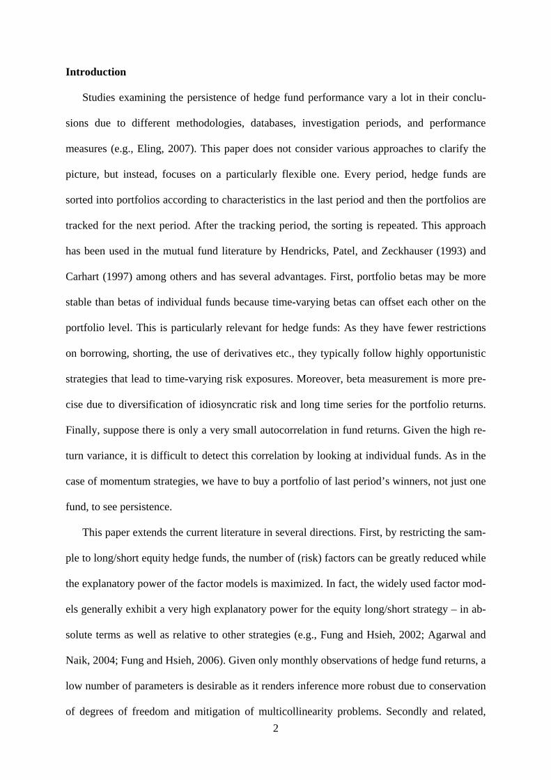
outperformed the market benchmark and had a long exposure to the market as Figure 1b

shows.

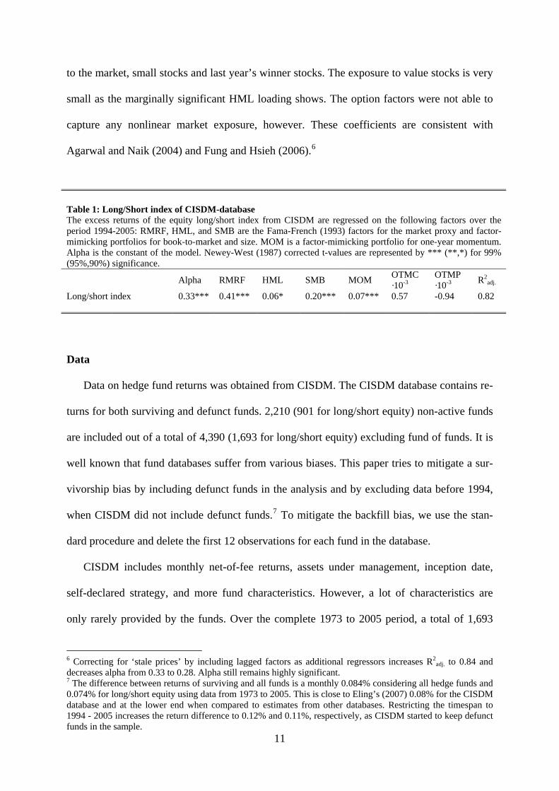
Figure 1a: Performance of long/short equity strategy The figure shows the S&P 500 and the CISDM long/short index and overall hedge fund index. All indi-ces are normalized to 100 in the beginning of 1994.

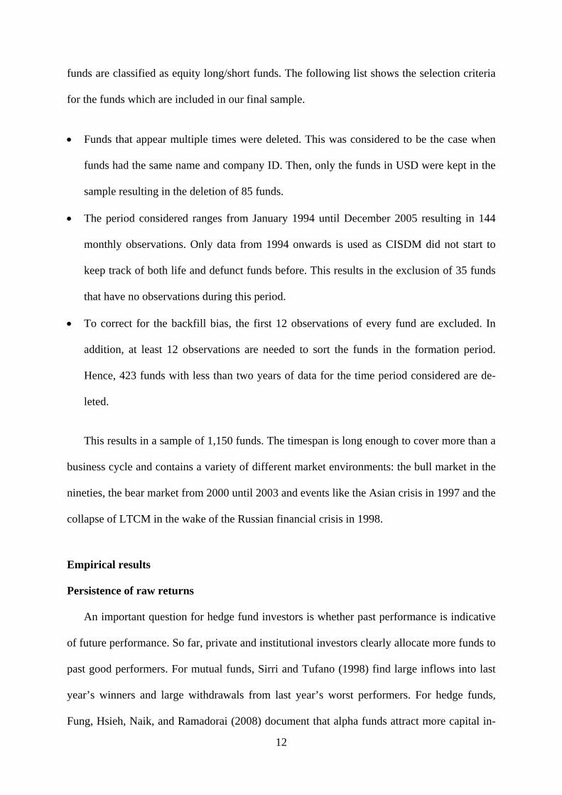
Figure 1b: Long/short equity versus market returnsThe scatterplot shows the S&P 500 monthly return versus the CISDM long/short index return from 1994 until end of 2005.

1994 1996 1998 2000 2002 2004 200650

100

150

200

250

300

350

400

450

-0.15 -0.1 -0.05 0 0.05 0.1-0.1

-0.05

0

0.05

0.1

return S&P 500

return long/short Index

S&P 500Long/short IndexHedge fund Index

As argued above, the market is an inappropriate benchmark. Applying the factor model

above shows that the index outperforms the more demanding multifactor benchmark. Table 1

displays a monthly outperformance of 0.33%. The factor loadings show significant exposure 10

11

to the market, small stocks and last year’s winner stocks. The exposure to value stocks is very

small as the marginally significant HML loading shows. The option factors were not able to

capture any nonlinear market exposure, however. These coefficients are consistent with

Agarwal and Naik (2004) and Fung and Hsieh (2006).6

Table 1: Long/Short index of CISDM-database The excess returns of the equity long/short index from CISDM are regressed on the following factors over the period 1994-2005: RMRF, HML, and SMB are the Fama-French (1993) factors for the market proxy and factor-mimicking portfolios for book-to-market and size. MOM is a factor-mimicking portfolio for one-year momentum. Alpha is the constant of the model. Newey-West (1987) corrected t-values are represented by *** (**,*) for 99% (95%,90%) significance. Alpha RMRF HML SMB MOM OTMC

·10-3OTMP ·10-3 R2

adj.

Long/short index 0.33*** 0.41*** 0.06* 0.20*** 0.07*** 0.57 -0.94 0.82

Data

Data on hedge fund returns was obtained from CISDM. The CISDM database contains re-

turns for both surviving and defunct funds. 2,210 (901 for long/short equity) non-active funds

are included out of a total of 4,390 (1,693 for long/short equity) excluding fund of funds. It is

well known that fund databases suffer from various biases. This paper tries to mitigate a sur-

vivorship bias by including defunct funds in the analysis and by excluding data before 1994,

when CISDM did not include defunct funds.7 To mitigate the backfill bias, we use the stan-

dard procedure and delete the first 12 observations for each fund in the database.

CISDM includes monthly net-of-fee returns, assets under management, inception date,

self-declared strategy, and more fund characteristics. However, a lot of characteristics are

only rarely provided by the funds. Over the complete 1973 to 2005 period, a total of 1,693

6 Correcting for ‘stale prices’ by including lagged factors as additional regressors increases R2

adj. to 0.84 and decreases alpha from 0.33 to 0.28. Alpha still remains highly significant. 7 The difference between returns of surviving and all funds is a monthly 0.084% considering all hedge funds and 0.074% for long/short equity using data from 1973 to 2005. This is close to Eling’s (2007) 0.08% for the CISDM database and at the lower end when compared to estimates from other databases. Restricting the timespan to 1994 - 2005 increases the return difference to 0.12% and 0.11%, respectively, as CISDM started to keep defunct funds in the sample.

12

funds are classified as equity long/short funds. The following list shows the selection criteria

for the funds which are included in our final sample.

• Funds that appear multiple times were deleted. This was considered to be the case when

funds had the same name and company ID. Then, only the funds in USD were kept in the

sample resulting in the deletion of 85 funds.

• The period considered ranges from January 1994 until December 2005 resulting in 144

monthly observations. Only data from 1994 onwards is used as CISDM did not start to

keep track of both life and defunct funds before. This results in the exclusion of 35 funds

that have no observations during this period.

• To correct for the backfill bias, the first 12 observations of every fund are excluded. In

addition, at least 12 observations are needed to sort the funds in the formation period.

Hence, 423 funds with less than two years of data for the time period considered are de-

leted.

This results in a sample of 1,150 funds. The timespan is long enough to cover more than a

business cycle and contains a variety of different market environments: the bull market in the

nineties, the bear market from 2000 until 2003 and events like the Asian crisis in 1997 and the

collapse of LTCM in the wake of the Russian financial crisis in 1998.

Empirical results

Persistence of raw returns

An important question for hedge fund investors is whether past performance is indicative

of future performance. So far, private and institutional investors clearly allocate more funds to

past good performers. For mutual funds, Sirri and Tufano (1998) find large inflows into last

year’s winners and large withdrawals from last year’s worst performers. For hedge funds,

Fung, Hsieh, Naik, and Ramadorai (2008) document that alpha funds attract more capital in-

13

flows than beta-only funds and Agarwal, Daniel, and Naik (2004) find that: "...funds with

persistently good (bad) performance attract larger (smaller) inflows compared to those that

show no persistence" (p. 2). Hence, in the presence of performance persistence, an investor

may be able to realize superior performance.

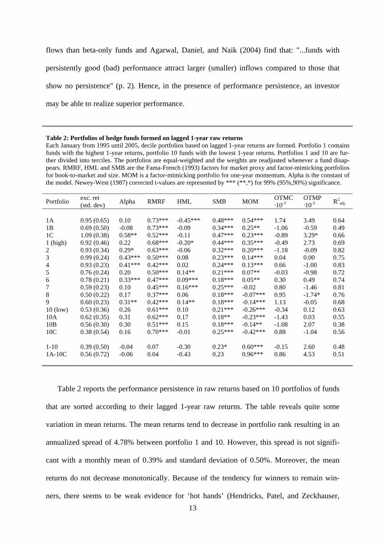
Table 2: Portfolios of hedge funds formed on lagged 1-year raw returns Each January from 1995 until 2005, decile portfolios based on lagged 1-year returns are formed. Portfolio 1 contains funds with the highest 1-year returns, portfolio 10 funds with the lowest 1-year returns. Portfolios 1 and 10 are fur-ther divided into terciles. The portfolios are equal-weighted and the weights are readjusted whenever a fund disap-pears. RMRF, HML and SMB are the Fama-French (1993) factors for market proxy and factor-mimicking portfolios for book-to-market and size. MOM is a factor-mimicking portfolio for one-year momentum. Alpha is the constant of the model. Newey-West (1987) corrected t-values are represented by *** (**,*) for 99% (95%,90%) significance.

Portfolio exc. ret (std. dev) Alpha RMRF HML SMB MOM OTMC

·10-3OTMP ·10-3 R2

adj.

1A 0.95 (0.65) 0.10 0.73*** -0.45*** 0.48*** 0.54*** 1.74 3.49 0.64 1B 0.69 (0.50) -0.08 0.73*** -0.09 0.34*** 0.25** -1.06 -0.59 0.49 1C 1.09 (0.38) 0.58** 0.52*** -0.11 0.47*** 0.23*** -0.89 3.29* 0.66 1 (high) 0.92 (0.46) 0.22 0.68*** -0.20* 0.44*** 0.35*** -0.49 2.73 0.69 2 0.93 (0.34) 0.29* 0.63*** -0.06 0.32*** 0.20*** -1.18 -0.09 0.82 3 0.99 (0.24) 0.43*** 0.50*** 0.08 0.23*** 0.14*** 0.04 0.00 0.75 4 0.93 (0.23) 0.41*** 0.42*** 0.02 0.24*** 0.13*** 0.66 -1.00 0.83 5 0.76 (0.24) 0.20 0.50*** 0.14** 0.21*** 0.07** -0.03 -0.98 0.72 6 0.78 (0.21) 0.33*** 0.47*** 0.09*** 0.18*** 0.05** 0.30 0.49 0.74 7 0.59 (0.23) 0.10 0.45*** 0.16*** 0.25*** -0.02 0.80 -1.46 0.81 8 0.50 (0.22) 0.17 0.37*** 0.06 0.18*** -0.07*** 0.95 -1.74* 0.76 9 0.60 (0.23) 0.31** 0.42*** 0.14** 0.18*** -0.14*** 1.13 -0.05 0.68 10 (low) 0.53 (0.36) 0.26 0.61*** 0.10 0.21*** -0.26*** -0.34 0.12 0.63 10A 0.62 (0.35) 0.31 0.62*** 0.17 0.18** -0.23*** -1.43 0.03 0.55 10B 0.56 (0.30) 0.30 0.51*** 0.15 0.18*** -0.14** -1.08 2.07 0.38 10C 0.38 (0.54) 0.16 0.70*** -0.01 0.25*** -0.42*** 0.88 -1.04 0.56 1-10 0.39 (0.50) -0.04 0.07 -0.30 0.23* 0.60*** -0.15 2.60 0.48 1A-10C 0.56 (0.72) -0.06 0.04 -0.43 0.23 0.96*** 0.86 4.53 0.51

Table 2 reports the performance persistence in raw returns based on 10 portfolios of funds

that are sorted according to their lagged 1-year raw returns. The table reveals quite some

variation in mean returns. The mean returns tend to decrease in portfolio rank resulting in an

annualized spread of 4.78% between portfolio 1 and 10. However, this spread is not signifi-

cant with a monthly mean of 0.39% and standard deviation of 0.50%. Moreover, the mean

returns do not decrease monotonically. Because of the tendency for winners to remain win-

ners, there seems to be weak evidence for ‘hot hands’ (Hendricks, Patel, and Zeckhauser,

1993) in equity long/short hedge funds for the 1-year horizon. This value is smaller than

Carhart’s (1997) annual 8% spread for mutual funds and Capocci, Corhay, and Huebner’s

(2005) 7.6% obtained by pooling all hedge fund strategies.

Our results indicate that, assuming normality for simplicity, the probability that last year’s

winners exhibit a positive return over the next month is 57.046.0

92.001)0( =⎟⎠

⎞⎜⎝

⎛ −−=>

TXP φ ,

where T is equal to 132. Moreover, the extreme portfolios have a higher return variance than

portfolios in the inner deciles, possibly due to higher leverage or generally riskier strategies.

This is consistent with Herzberg and Mozes (2003) who find that the funds with the highest

past returns have the highest volatility.

When we alternatively adjust the raw returns for risk by using an alpha from a Carhart

(1997) four factor model, the spread in performance disappears. In fact, portfolio 10 has a

(insignificantly) higher alpha than portfolio 1. It is interesting to see that the significant alphas

are located in the inner deciles (portfolios 3, 4, 6, and 9) while the portfolio of last year’s win-

ners does not outperform against the benchmark model. Instead, they show more return varia-

tion that eventually places them in more extreme deciles. The alpha portfolios, however, show

relatively little return variance. This indicates that, on average, alpha funds are characterized

not only by high returns but also low volatility.8 In fact, portfolios 3, 4, and 6 have the three

highest Sharpe Ratios and portfolio 9 the sixth highest Sharpe Ratio (not reported).

Looking at the factor loadings, the coefficient on RMRF is around 0.5 and shows no spe-

cific pattern. With respect to HML, there seems to be a tendency of last year’s winners to be

more growth-oriented while other deciles have more of a value focus, though coefficients are

generally small and insignificant. More revealing is the pattern of the SMB coefficients. All

portfolios have positive exposure, which confirms earlier findings that long/short funds are

8 Strictly speaking, we cannot infer anything about the volatility of the underlying funds by looking at portfolio volatility because it is influenced by the covariance terms.

14

15

small cap oriented (Agarwal and Naik, 2004; Fung and Hsieh, 2006). Last year’s winners are

strongly exposed to small cap stocks. This exposure decreases in the decile numbering but

remains positive. The spread between portfolio 1 and 10 is marginally significant and explains

some of the spread in raw returns: Some funds continue to earn higher returns because they

are more exposed to small stocks and capture their premium. The largest spread, however, is

in the momentum loadings. There is a monotonous decrease from 0.35 for portfolio 1 to -0.26

for portfolio 10 with the extreme portfolios 1A and 10C showing the strongest exposure. Giv-

en the monthly return spread of 0.39% and the mean of the momentum factor of 0.84%, the

spread in the loading of 0.6 more than accounts for the difference in returns. The momentum

factor explains the return spread by identifying last year’s winners as the holders of last year’s

winning stocks. The identified patterns for SMB and MOM are very similar to mutual funds,

where Carhart (1997) reports a spread of 0.30 for SMB and 0.38 for MOM between portfolio

1 and 10. The option strategies add very few explanatory power, are rarely significant, and

show no specific pattern across the deciles. This confirms the evidence on the index level and

shows that better performing long/short equity hedge funds on average do not differ in

nonlinear market exposure compared to worse performing funds.

Overall, the model does a good job at explaining the returns of portfolios based on lagged

fund returns. The R² ranges from 0.63 to 0.83 for the decile portfolios. This is lower than Car-

hart’s four factor model for mutual funds, where the R²s are above 0.9. However, this is not

surprising given the diversity of individual hedge fund strategies for this particular style.

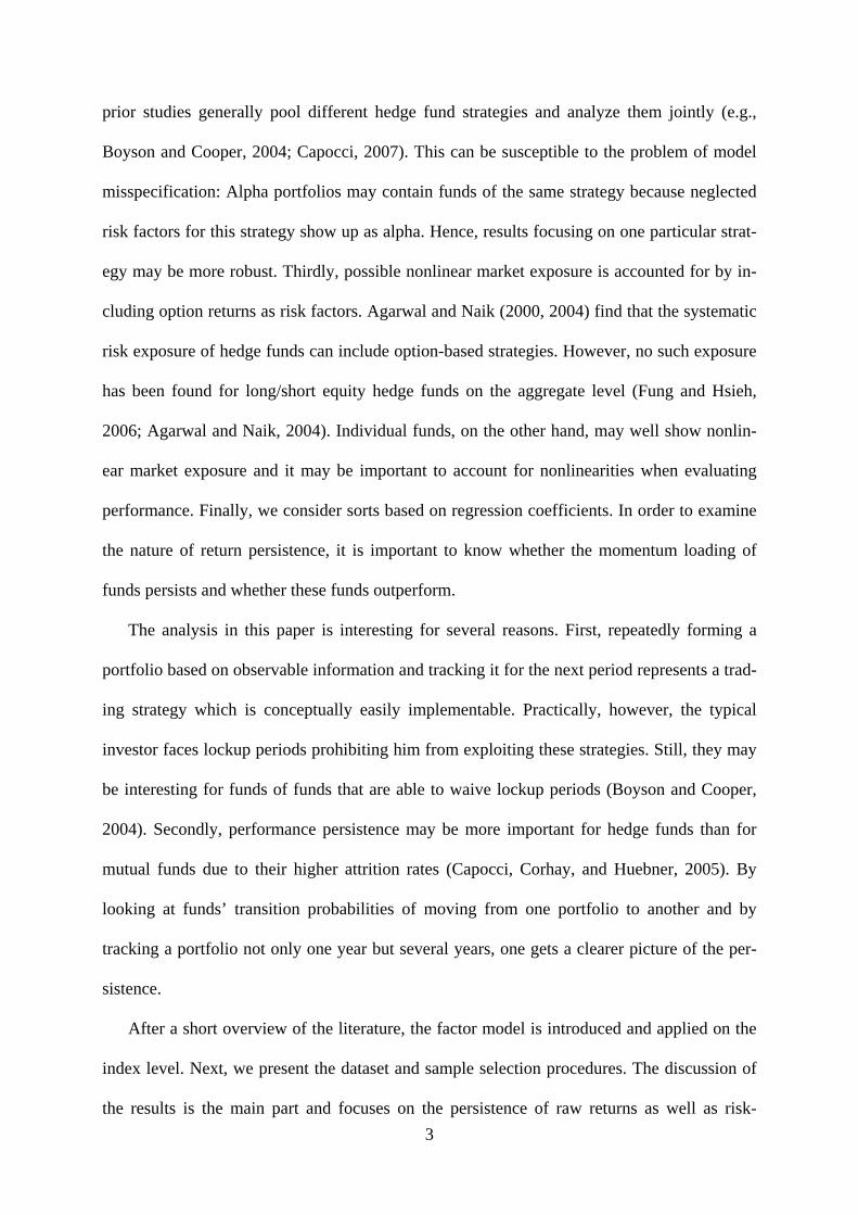
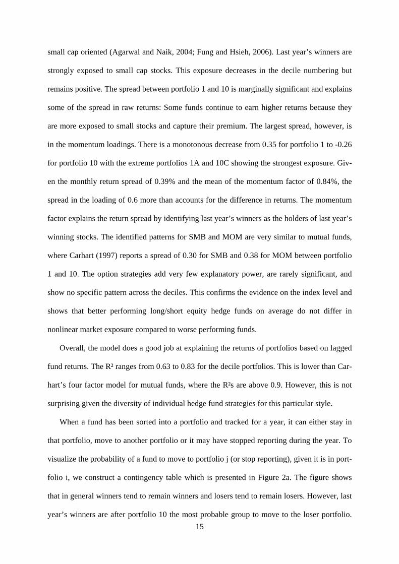
When a fund has been sorted into a portfolio and tracked for a year, it can either stay in

that portfolio, move to another portfolio or it may have stopped reporting during the year. To

visualize the probability of a fund to move to portfolio j (or stop reporting), given it is in port-

folio i, we construct a contingency table which is presented in Figure 2a. The figure shows

that in general winners tend to remain winners and losers tend to remain losers. However, last

year’s winners are after portfolio 10 the most probable group to move to the loser portfolio.

The same is true for last year’s losers: They are after portfolio 1 the most probable group to

end up as this year’s winners. This is in accordance with the high return variance of the ex-

treme portfolios. There is also the tendency of the inner decile funds to remain in the inner

deciles, which is consistent with their low return variance. The probability of stopping to re-

port shows an increasing pattern with respect to last year’s ranking and is highest for last

year’s losers. This is in line with Liang (2000), Brown, Goetzmann, and Park (2001), and Ba-

quero, Jenke, and Verbeek (2004) who find that hedge funds with low past performance are

likely candidates for liquidation. Overall, however, hedge funds move a lot between portfolio

deciles and the detected patterns are not very strong.

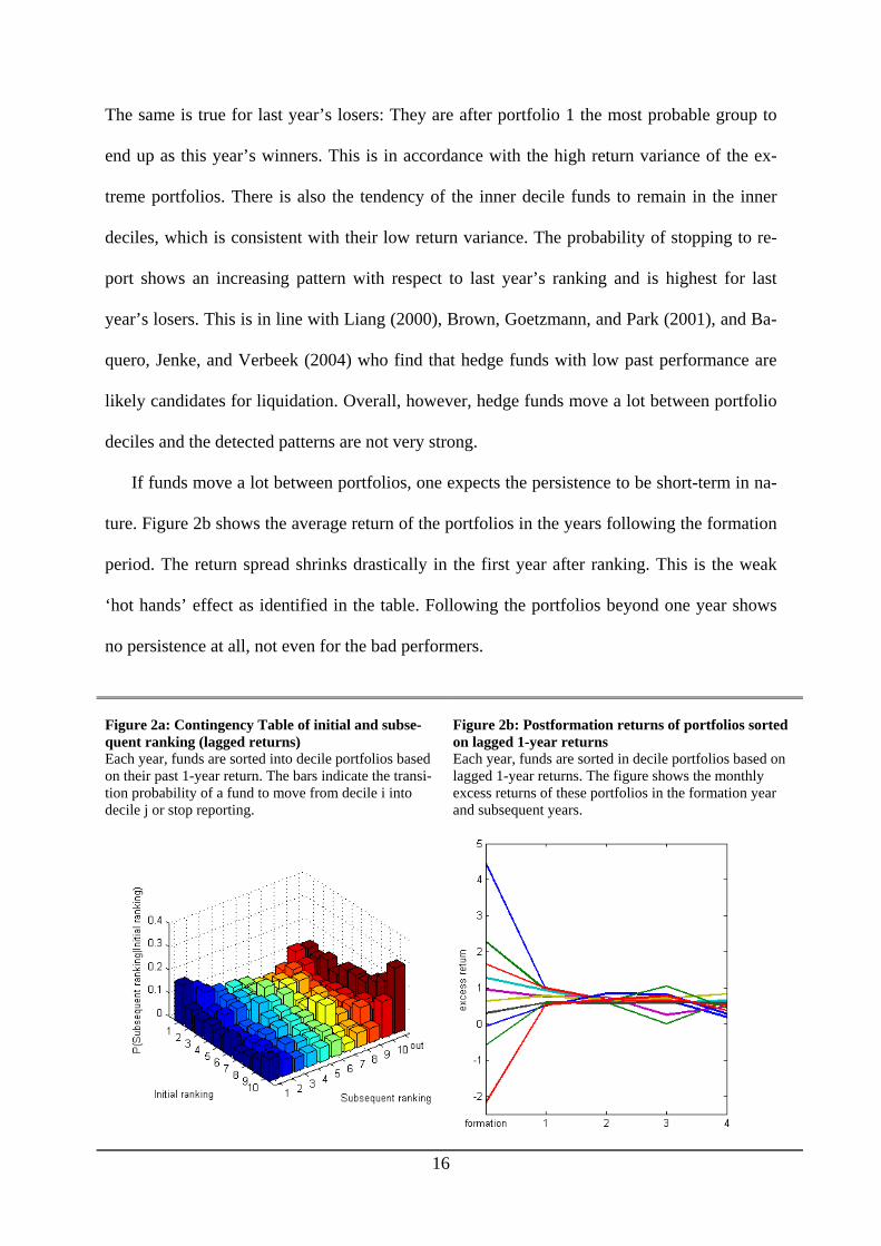
If funds move a lot between portfolios, one expects the persistence to be short-term in na-

ture. Figure 2b shows the average return of the portfolios in the years following the formation

period. The return spread shrinks drastically in the first year after ranking. This is the weak

‘hot hands’ effect as identified in the table. Following the portfolios beyond one year shows

no persistence at all, not even for the bad performers.

16

Figure 2a: Contingency Table of initial and subse-quent ranking (lagged returns) Each year, funds are sorted into decile portfolios based on their past 1-year return. The bars indicate the transi-tion probability of a fund to move from decile i into decile j or stop reporting.

Figure 2b: Postformation returns of portfolios sorted on lagged 1-year returns Each year, funds are sorted in decile portfolios based on lagged 1-year returns. The figure shows the monthly excess returns of these portfolios in the formation year and subsequent years.

17

Detection and persistence of alpha

Forming portfolios based on lagged returns does not seem to be a useful way to detect al-

pha portfolios. Instead, one would like a characteristic that provides a monotonous change of

alpha across the deciles. Hence, we alternatively sort funds into portfolios based on lagged

alphas.9 To provide reasonable estimates, alpha is calculated using the past 24 months of data.

Table 3 provides the regression results for the decile portfolios with portfolio 1 containing the

funds with the highest lagged alpha and portfolio 10 containing the funds with the lowest

lagged alpha.

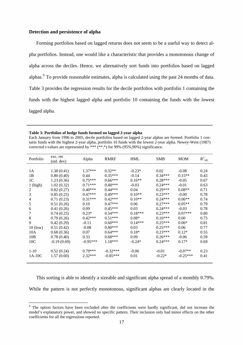
Table 3: Portfolios of hedge funds formed on lagged 2-year alpha Each January from 1996 to 2005, decile portfolios based on lagged 2-year alphas are formed. Portfolio 1 con-tains funds with the highest 2-year alpha, portfolio 10 funds with the lowest 2-year alpha. Newey-West (1987) corrected t-values are represented by *** (**,*) for 99% (95%,90%) significance.

Portfolio exc. ret (std. dev) Alpha RMRF HML SMB MOM R2

adj.

1A 1.38 (0.41) 1.37*** 0.32** -0.23* 0.02 -0.08 0.24 1B 0.80 (0.40) 0.44 0.35*** -0.14 0.34*** 0.15** 0.43 1C 1.23 (0.36) 0.75*** 0.66*** 0.16** 0.28*** -0.05 0.67 1 (high) 1.02 (0.32) 0.71*** 0.48*** -0.03 0.24*** -0.01 0.63 2 0.82 (0.27) 0.40*** 0.44*** 0.04 0.29*** 0.08** 0.71 3 0.85 (0.25) 0.47*** 0.49*** 0.10** 0.23*** -0.00 0.78 4 0.71 (0.23) 0.31*** 0.42*** 0.10** 0.24*** 0.06** 0.74 5 0.51 (0.26) 0.10 0.47*** 0.06 0.27*** 0.05** 0.79 6 0.41 (0.26) 0.09 0.45*** 0.03 0.24*** -0.03 0.78 7 0.74 (0.25) 0.23* 0.54*** 0.18*** 0.23*** 0.07*** 0.80 8 0.79 (0.26) 0.42*** 0.51*** 0.08* 0.16*** 0.00 0.75 9 0.42 (0.29) -0.11 0.60*** 0.14*** 0.25*** 0.06* 0.81 10 (low) 0.51 (0.42) -0.08 0.80*** 0.03 0.25*** 0.06 0.77 10A 0.68 (0.36) 0.07 0.64*** 0.18* 0.23*** 0.12* 0.55 10B 0.78 (0.40) 0.33 0.68*** 0.09 0.26*** -0.06 0.59 10C -0.19 (0.69) -0.95*** 1.18*** -0.24* 0.24*** 0.17* 0.69 1-10 0.52 (0.24) 0.79*** -0.32*** -0.06 -0.01 -0.07** 0.23 1A-10C 1.57 (0.60) 2.32*** -0.85*** 0.01 -0.22* -0.25*** 0.41

This sorting is able to identify a sizeable and significant alpha spread of a monthly 0.79%.

While the pattern is not perfectly monotonous, significant alphas are clearly located in the

9 The option factors have been excluded after the coefficients were hardly significant, did not increase the model’s explanatory power, and showed no specific pattern. Their inclusion only had minor effects on the other coefficients for all the regressions reported.

18

portfolios containing the funds with high lagged alpha. Persistence in alpha is especially pro-

nounced for the extreme portfolios 1A and 10C. However, portfolio 1A seems to be poorly

explained by the factors.

The table also shows that the portfolios with significant alphas have the highest returns. In

fact, sorting based on lagged alpha produces a larger return spread than a sorting based on

lagged returns. The spread is a significant monthly 0.52% compared to an insignificant 0.39%

for the portfolios based on lagged returns. Hence, lagged alpha seems to provide more infor-

mation about both future alpha and future raw returns. With respect to factor exposure, alpha

portfolios are generally less exposed to the market. This is also shown by the 1 minus 10 port-

folio at the bottom of Table 3 where the difference in the RMRF-coefficient is reported to be

negative and significant at the 1% level.

Alternatively, we sort the funds based on lagged 3-year alphas. However, the alpha spread

between portfolio 1 and 10 decreases to an insignificant 0.44%. There are at least two poten-

tial explanations for this decrease. First, by requiring funds to have at least three years of data

to estimate 3-year alphas, the portfolios contain less funds and the estimates become less pre-

cise. In fact, the R² for portfolio 1 gets as low as 0.44. Secondly, a fund’s alpha three years

ago may provide few information about today’s alpha. Sorting on lagged 1-year alpha, on the

other hand, gives a significant 0.67% spread in alpha between portfolio 1 and 10. However,

the funds’ alphas are estimated very imprecisely and the portfolio alphas show no monoto-

nous pattern. This suggests that alpha persistence is only a short-run phenomenon. The fol-

lowing passage takes a closer look at this.

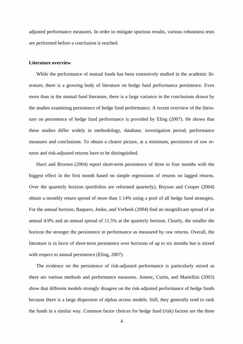
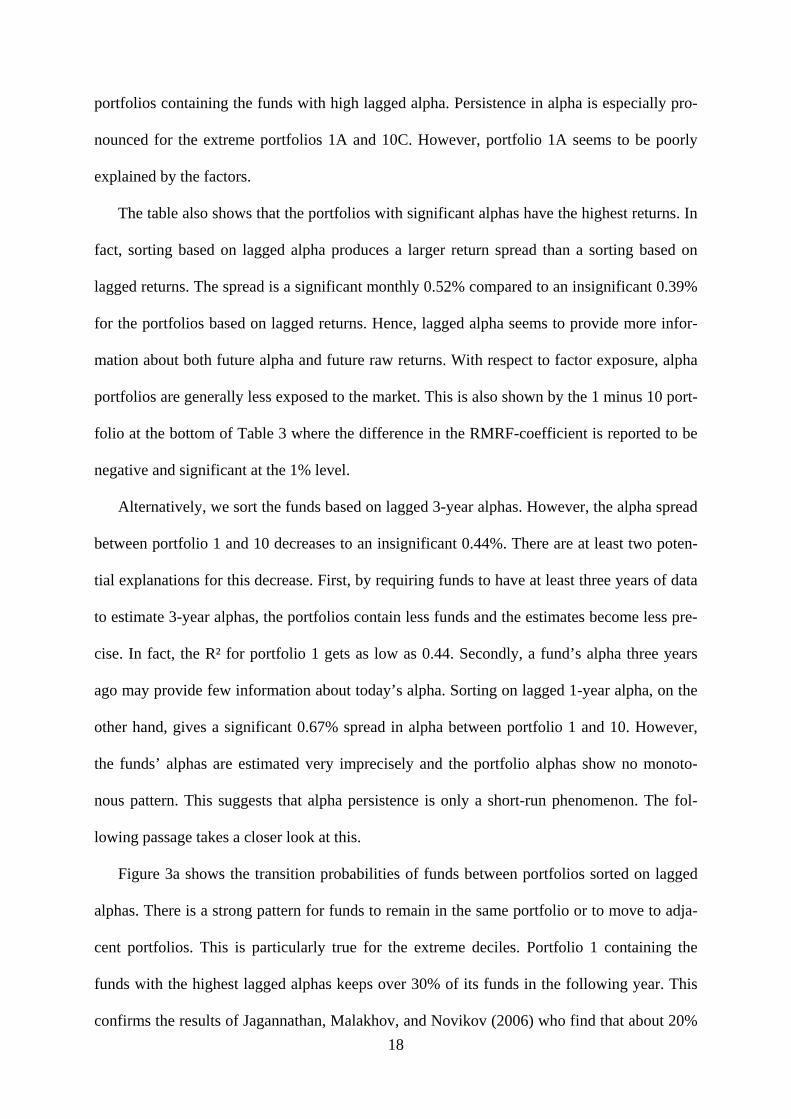
Figure 3a shows the transition probabilities of funds between portfolios sorted on lagged

alphas. There is a strong pattern for funds to remain in the same portfolio or to move to adja-

cent portfolios. This is particularly true for the extreme deciles. Portfolio 1 containing the

funds with the highest lagged alphas keeps over 30% of its funds in the following year. This

confirms the results of Jagannathan, Malakhov, and Novikov (2006) who find that about 20%

of abnormal performance relative to the style benchmark over a three-year period spills over

to the next three-year period. This persistence is stronger among top funds than among bottom

funds. Moreover, the figure shows that it is very unlikely for a high-alpha fund to become a

low-alpha fund in the subsequent year or vice versa. This stands in sharp contrast to high-

return funds as shown above. The probability that a fund stops reporting is decreasing in

lagged alpha. This confirms the findings of Fung, Hsieh, and Naik (2007) who show that al-

pha-funds exhibit substantially lower liquidation rates than beta-only funds.

Figure 3a: Contingency table of initial and subse-quent ranking (lagged alpha)

Figure 3b: Postformation alpha of portfolios sorted on lagged 2-year alpha

Figure 3b shows the alphas of the portfolios over several years. Similar to sorting portfo-

lios based on lagged returns, the spread decreases after the formation period though not as

strongly. There is clearly more persistence in alpha than in raw returns for the first year. As in

Kosowski, Naik, and Teo (2005) abnormal performance is significant and persists over one

year. While much of the persistence in alpha is gone after one year, the worst performers con-

tinue to underperform for two years. The alpha spread even widens to 0.97%. But both the

winner and loser portfolios have alphas insignificantly different from zero after the tracking

year and the alpha spread is only significant at the 5%-level. Hence, portfolios based on

19

20

lagged alphas should be reformed annually as there is no outperformance two, three, and four

years after picking the high alpha funds.

The results are similar when we alternatively sort the funds based on the t-value of lagged

alphas which is the same as sorting based on the appraisal ratio. This sorting procedure identi-

fies a highly significant alpha spread of 0.84% and a return spread of 0.58%. Carhart (1997),

however, argues that using the same model for sorting and performance evaluation can pick

up a model bias. For example, if the factor exposures are estimated too low or too high for a

fund, this shows up as persistent over- or underperformance relative to the factor model. The

problem is similar to an omitted factor. Hence, it is important to keep in mind this potential

shortcoming when interpreting the results reported in this section.

Finally, we sort the funds into portfolios based on lagged Sharpe Ratios. This does a better

job at detecting alpha portfolios than sorting based on raw returns or return variance and gen-

erates a decreasing pattern in alphas across deciles. In contrast, the reported results based on

alpha sorting are stronger. For space reasons, we do not report the results from the Sharpe

Ratio sorting.10

Robustness Checks

Subperiod analysis

In order to assess the robustness of these results, we conduct the analyses for subperiods.

Prior research examines the relation between hedge fund performance and market conditions.

Using a conditional benchmark, Kat and Miffre (2002) conclude that abnormal performance is

counter-cyclical. Capocci, Corhay, and Huebner (2005), however, find that hedge funds show

stronger outperformance in bullish times. Here, March 2000 is set as the cut-off point that

divides the sample into a bull market period from January 1994 to March 2000 and a period

with bear market from April 2000 to December 2005. This also allows the factor loadings to

10 These results are available from the authors upon request.

21

vary between these two samples. In fact, Kosowski, Naik, and Teo (2005) find a breakpoint in

the year 2000 for most hedge fund return indices.

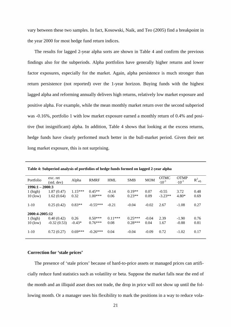
The results for lagged 2-year alpha sorts are shown in Table 4 and confirm the previous

findings also for the subperiods. Alpha portfolios have generally higher returns and lower

factor exposures, especially for the market. Again, alpha persistence is much stronger than

return persistence (not reported) over the 1-year horizon. Buying funds with the highest

lagged alpha and reforming annually delivers high returns, relatively low market exposure and

positive alpha. For example, while the mean monthly market return over the second subperiod

was -0.16%, portfolio 1 with low market exposure earned a monthly return of 0.4% and posi-

tive (but insignificant) alpha. In addition, Table 4 shows that looking at the excess returns,

hedge funds have clearly performed much better in the bull-market period. Given their net

long market exposure, this is not surprising.

Table 4: Subperiod analysis of portfolios of hedge funds formed on lagged 2-year alpha

Portfolio exc. ret (std. dev) Alpha RMRF HML SMB MOM OTMC

·10-3OTMP ·10-3 R2

adj.

1996:1 – 2000:3 1 (high) 1.87 (0.47) 1.15*** 0.45** -0.14 0.19** 0.07 -0.55 3.72 0.48 10 (low) 1.62 (0.64) 0.32 1.00*** 0.06 0.23** 0.09 -3.23** 4.80* 0.69 1-10 0.25 (0.42) 0.83** -0.55*** -0.21 -0.04 -0.02 2.67 -1.08 0.27 2000:4-2005:12 1 (high) 0.40 (0.42) 0.26 0.50*** 0.11*** 0.25*** -0.04 2.39 -1.90 0.76 10 (low) -0.32 (0.53) -0.43* 0.76*** 0.08 0.28*** 0.04 1.67 -0.88 0.81 1-10 0.72 (0.27) 0.69*** -0.26*** 0.04 -0.04 -0.09 0.72 -1.02 0.17 Correction for ‘stale prices’

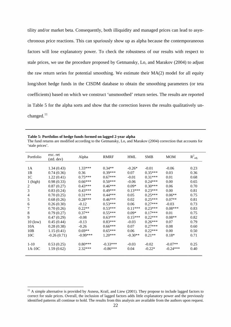
The presence of ‘stale prices’ because of hard-to-price assets or managed prices can artifi-

cially reduce fund statistics such as volatility or beta. Suppose the market falls near the end of

the month and an illiquid asset does not trade, the drop in price will not show up until the fol-

lowing month. Or a manager uses his flexibility to mark the positions in a way to reduce vola-

22

tility and/or market beta. Consequently, both illiquidity and managed prices can lead to asyn-

chronous price reactions. This can spuriously show up as alpha because the contemporaneous

factors will lose explanatory power. To check the robustness of our results with respect to

stale prices, we use the procedure proposed by Getmansky, Lo, and Marakov (2004) to adjust

the raw return series for potential smoothing. We estimate their MA(2) model for all equity

long/short hedge funds in the CISDM database to obtain the smoothing parameters (or teta

coefficients) based on which we construct ‘unsmoothed’ return series. The results are reported

in Table 5 for the alpha sorts and show that the correction leaves the results qualitatively un-

changed.11

Table 5: Portfolios of hedge funds formed on lagged 2-year alpha The fund returns are modified according to the Getmansky, Lo, and Marakov (2004) correction that accounts for ‘stale prices’.

Portfolio exc. ret (std. dev) Alpha RMRF HML SMB MOM R2

adj.

1A 1.34 (0.43) 1.33*** 0.34** -0.26* -0.01 -0.06 0.23 1B 0.74 (0.36) 0.36 0.39*** 0.07 0.35*** 0.03 0.36 1C 1.22 (0.41) 0.75*** 0.67*** -0.01 0.31*** 0.01 0.68 1 (high) 0.98 (0.33) 0.66*** 0.50*** -0.06 0.24*** 0.00 0.65 2 0.87 (0.27) 0.43*** 0.46*** 0.09* 0.30*** 0.06 0.70 3 0.83 (0.24) 0.43*** 0.49*** 0.13*** 0.23*** 0.00 0.81 4 0.70 (0.25) 0.31*** 0.44*** 0.05 0.25*** 0.06** 0.75 5 0.68 (0.26) 0.28*** 0.46*** 0.02 0.25*** 0.07** 0.81 6 0.26 (0.30) -0.12 0.53*** 0.06 0.27*** -0.03 0.73 7 0.70 (0.26) 0.22** 0.53*** 0.11*** 0.23*** 0.08*** 0.83 8 0.79 (0.27) 0.37** 0.55*** 0.09* 0.17*** 0.01 0.75 9 0.47 (0.29) -0.08 0.63*** 0.15*** 0.22*** 0.08** 0.82 10 (low) 0.45 (0.44) -0.13 0.83*** -0.03 0.26*** 0.07 0.79 10A 0.28 (0.38) -0.26 0.66*** 0.07 0.27*** 0.08 0.60 10B 1.15 (0.41) 0.69** 0.65*** 0.06 0.22*** 0.00 0.50 10C -0.26 (0.71) -0.99*** 1.20*** -0.30** 0.21** 0.18* 0.71 1-10 0.53 (0.25) 0.80*** -0.33*** -0.03 -0.02 -0.07** 0.25 1A-10C 1.59 (0.62) 2.32*** -0.86*** 0.04 -0.22* -0.24*** 0.40

11 A simple alternative is provided by Asness, Krail, and Liew (2001). They propose to include lagged factors to correct for stale prices. Overall, the inclusion of lagged factors adds little explanatory power and the previously identified patterns all continue to hold. The results from this analysis are available from the authors upon request.

23

Conclusion

This paper investigates the performance persistence of equity long/short hedge funds. We

find returns to show very little persistence at the annual horizon irrespective of the length of

the formation period. In addition, the observed persistence can be fully explained by factor

exposures. In fact, it is mainly driven by holdings of last year’s winner stocks. Hence, funds

with the highest return last period are generally no alpha-funds. Moreover, best and worst

performing funds tend to switch their places often as they are very volatile.

However, there are more promising criteria to select outperforming funds. Sharpe Ratio,

market beta and in particular alpha are more useful characteristics to sort funds because they

are more persistent than raw returns. Although not reported in the paper, we find that sorting

on lagged Sharpe Ratio identifies portfolios with the highest Sharpe Ratio which are also

more likely to have alpha. Sorting on lagged market beta or alpha identifies the largest and

most significant alpha spread over the subsequent period. Past alpha also provides the most

information about future returns by discovering the most significant spread in raw returns.

These selection strategies are associated with less risk than selection based on raw returns.

Funds with high alpha are very unlikely to have a low alpha in the next period, instead, they

will likely stay in the same or adjacent portfolio. Also, there is more persistence in alpha at

the annual horizon. However, no persistence in alpha has been detected for longer horizons

except that funds with the lowest alpha continue to have the lowest alpha for two years.

However, there are at least three reasons that render such trading strategies impractical.

First, the option of going short a portfolio of hedge funds to get the alpha spread is not avail-

able. Secondly, the transaction and administrative costs of implementing such a strategy may

outweigh its benefits. Thirdly, lockup or redemption periods imposed by funds can make fre-

quent disinvestment impossible. However, selecting funds with the highest lagged alpha al-

ready produces a significant monthly alpha of 0.71% while the spread between portfolio 1 and

24

10 is 0.78%. Going short portfolio 10 is therefore not necessary to get most of the benefit.12

Secondly, the annual frequency of reforming the portfolios is relatively low. This makes the

strategies more feasible with respect to transaction costs and lockup periods, especially for

funds of funds facing more favorable conditions than individual investors.

References

Agarwal, V., Daniel, N. and Naik, N. (2004) ‘Flows, performance, and managerial incentives

in hedge funds’, Working Paper, Georgia State University.

Agarwal, V. and Naik, N. (2000) ‘Multi-period performance persistence analysis of hedge

funds’, Journal of Financial and Quantitative Analysis, 35(3), 327-342.

Agarwal, V. and Naik, N. (2004) ‘Risks and portfolio decisions involving hedge funds,’ Re-

view of Financial Studies, 17(1), 63-98.

Amenc, N., Curtis, S. and Martellini, L. (2003) ‘The alpha and omega of hedge fund perform-

ance measurement’, Working Paper, EDHEC Business School.

Asness, C., Krail, R. and Liew, J. (2001) ‘Do hedge funds hedge?’ Journal of Portfolio Man-

agement, 28(Fall), 6-19.

Baquero, G., Jenke R. and Verbeek, M. (2004) ‘Survival, look-ahead bias and the persistence

in hedge fund performance’, Working Paper, ESMT European School of Management

and Technology.

Boyson, N. and Cooper, M. (2004) ‘Do hedge funds exhibit performance persistence? A new

approach’, Working Paper, Northeastern University.

Brown, S., Goetzmann, W. and Park, J. (2001) ‘Careers and survival: Competition and risk in

the hedge fund and CTA industry’, Journal of Finance, 56(5), 1869-1886.

Capocci, D. (2007) ‘The sustainability in hedge fund performance: New insights’, Working

Paper, HEC Université de Liège.

Capocci, D., Corhay, A. and Huebner, G. (2005) ‘Hedge fund performance and persistence in

bull and bear markets’, European Journal of Finance, 11(5), 361-392.

Carhart, M. (1997) ‘On persistence in mutual fund performance’, Journal of Finance, 52(1),

57-82.

Davis, J. (2001) ‘Mutual fund performance and manager style’, Financial Analysts Journal,

57(1), 19-27.

12 However, using the more recent subsample (2000-2005), the largest part of the alpha spread comes from the negative alpha of portfolio 10.

25

Edwards F. and Caglayan, M. (2001) ‘Hedge fund performance and manager skill’, Journal of

Futures Markets, 21(11), 1003-1028.

Eling, M. (2007) ‘Does hedge fund performance persist? Overview and new empirical evi-

dence’, Working Paper, University of St. Gallen.

Fama, E. and French, K. (1993) ‘Common risk factors in the returns on bonds and stocks’,

Journal of Financial Economics, 33(1), 3-53.

Fung, W. and Hsieh, D. (2001) ‘The risk in hedge fund strategies: Theory and evidence from

trend followers’, Review of Financial Studies, 14(2), 313-341.

Fung, W. and Hsieh, D. (2004) ‘Hedge fund benchmarks: A risk based approach’, Financial

Analyst Journal, 60(5), 65-80.

Fung, W. and Hsieh, D. (2006) ‘The risk in hedge fund strategies: Theory and evidence from

long/short equity hedge funds’, Working Paper, Duke University.

Fung, W., Hsieh, D., Naik, N. and Ramadorai, T. (2008) ‘Hedge Funds: Performance, Risk

and Capital Formation’, Journal of Finance, forthcoming.

Getmansky, M., Lo, A. and Makarov, I. (2004) ‘An Econometric Model of Serial Correlation

and Illiquidity in Hedge Fund Returns’, Journal of Financial Economics, 74(3), 529-

610.

Glosten, L. and Jagannathan, R. (1994) ‘A contingent claim approach to performance evalua-

tion’, Journal of Empirical Finance, 1(2), 133-160.

Harri, A. and Brorsen, B. (2004) ‘Performance persistence and the source of returns for hedge

funds’, Applied Financial Economics, 14(2), 131-141.

Hendricks, D., Patel, P. and Zeckhauser, R. (1993) ‘Hot hands in mutual funds: Short-run

persistence of relative performance, 1974-1988’, Journal of Finance, 48(1), 93-130.

Herzberg, M. and Mozes, H. (2003) ‘The Persistence of hedge fund risk: Evidence and impli-

cations for investors’, Journal of Alternative Investments, 6(Fall), 22-42.

Jagannathan, R., Malakhov, A. and Novikov, D. (2006) ‘Do Hot Hands exist among hedge

fund managers? An Empirical Evaluation’, Working Paper, Northwestern University.

Jegadeesh, N. and Titman, S. (1993) ‘Returns to buying winners and selling losers: Implica-

tions for stock market efficiency’, Journal of Finance, 48(1), 65-91.

Kat, H. and Miffre, J. (2002) ‘Performance evaluation and conditioning information: The case

of hedge funds’, Working Paper, University of Reading.

Kosowski, R., Naik, N. and Teo, M. (2005) ‘Do hedge funds deliver alpha? A bayesian and

bootstrap analysis’, Working Paper, London Business School.

26

Kosowski, R., Timmermann, A., Wermers, R. and White, H. (2006) ‘Can mutual fund “stars”

really pick stocks? New evidence from a bootstrap analysis’, Journal of Finance, 61(6),

2551-2595.

Liang, B. (2000) ‘Hedge funds: The living and the dead’, Journal of Financial and Quantita-

tive Analysis, 35(3), 309-326.

Naik, N., Ramadorai, T. and Strömqvist, M. (2007) ‘Capacity constraints and hedge fund

strategy returns’, European Financial Management, 13(2), 239-256.

Newey, W. and West, K. (1987) ‘A simple, positive semi-definite, heteroskedasticity and au-

tocorrelation consistent covariance matrix’, Econometrica, 55(3), 703-08.

Sirri, E. and Tufano, P. (1998) ‘Costly search and mutual fund flows’, Journal of Finance,

53(5), 1589-1622.