Embed Size (px)
Citation preview

The Pennsylvania State University
The Graduate School
Department of Mechanical and Nuclear Engineering
HELICOPTER GEARBOX ISOLATION USING PERIODICALLY
LAYERED FLUIDIC ISOLATORS
A Thesis in
Mechanical Engineering
by
Joseph Thomas Szefi
2003 Joseph Thomas Szefi
Submitted in Partial Fulfillmentof the Requirements
for the Degree of
Doctor of Philosophy
August 2003
The Pennsylvania State University

We approve the thesis of Joseph Thomas Szefi.
Date of Signature
Edward C. SmithAssociate Professor of Aerospace EngineeringThesis Co-AdvisorCo-chair of Committee
George A. LesieutreProfessor of Aerospace EngineeringThesis Co-AdvisorCo-chair of Committee
Kon-Well WangWilliam E. Diefenderfer Chaired Professor in
Mechanical EngineeringCo-chair of Committee
Gary H. KoopmannDistinguished Professor of Mechanical
Engineering
Richard C. BensonProfessor of Mechanical EngineeringHead of the Department of Mechanical
Engineering

iii
ABSTRACT
In rotorcraft transmissions, vibration generation by meshing gear pairs is a
significant source of vibration and cabin noise. This high-frequency gearbox noise is
primarily transmitted to the fuselage through rigid connections, which do not appreciably
attenuate vibratory energy. The high-frequency vibrations typically include discrete
gear-meshing frequencies in the range of 500 – 2000 Hz, and are often considered
irritating and can reduce pilot effectiveness and passenger comfort.
Periodically-layered isolators were identified as potential passive attenuators of
these high frequency vibrations. Layered isolators exhibit transmissibility “stop bands,”
or frequency ranges in which there is very low transmissibility. An axisymmetric model
was developed to accurately predict the location of these stop bands for isolators in
compression. A Ritz approximation method was used to model the axisymmetric elastic
behavior of layered cylindrical isolators. This model of layered isolators was validated
with experiments.
The physical design constraints of the proposed helicopter gearbox isolators were
then estimated. Namely, constraints associated with isolator mass, axial stiffness,
geometry, and elastomeric fatigue were determined. The passive performance limits of
layered isolators were then determined using a design optimization methodology
employing a simulated annealing algorithm. The results suggest that layered isolators
cannot always meet frequency targets given a certain set of design constraints.

iv
Many passive and active design enhancements were considered to address this
problem, and the use of embedded inertial amplifiers was found to exhibit a combination
of advantageous effects. The first benefit was a lowering of the beginning stop band
frequency, and thus a widening of the original stop band. The second was a tuned
absorber effect, where the elastomer layer stiffness and the amplified tuned mass
combined to act as a vibration absorber within the stop band. The use of embedded fluid
elements was identified as an efficient means of implementing inertial amplification.
When elastomer layers are compressed quasi-statically, the actual measured axial
stiffness is quite higher the than one-dimensional stiffness predicted on the basis of a
Young’s modulus. Because of this effect, layered isolators can be designed to
accommodate the high axial stiffnesses required for helicopter gearbox supports, while
also providing broadband high frequency attenuation.

TABLE OF CONTENTS
LIST OF FIGURES..................................................................................................viii
LIST OF TABLES ...................................................................................................xiii
ACKNOWLEDGMENTS ........................................................................................xv
Chapter 1 INTRODUCTION..................................................................................1
1.1 Background and Motivation.........................................................................11.2 Literature Review ........................................................................................5
1.2.1 Sources of High Frequency Noise Inside Helicopter Cabins...............51.2.2 Rotorcraft Interior Noise Control .......................................................9
1.2.2.1 Passive Treatments...................................................................91.2.2.2 Active Noise Cancellation........................................................111.2.2.3 Active Structural Vibration Control..........................................121.2.2.4 Minimum Noise Transmission from Gearbox...........................13
1.2.3 Periodically Layered Media for High Frequency Isolation..................161.3 Research Objectives.....................................................................................17
Chapter 2 PERIODICALLY LAYERED ISOLATORS FOR HIGHFREQUENCY ISOLATION .............................................................................21
2.1 One Dimensional Finite Elements Analysis .................................................212.2 Three Dimensional Finite Element Analysis ................................................23
2.2.1 One Dimensional Stiffness Correction Factors ...................................262.2.1.1 Shape Factor Influence on Higher Modes.................................30
2.2.2 Table Look-up Methodology..............................................................332.3 Axisymmetric Approximation Method.........................................................34
2.3.1 Natural Frequency of 3-D Cylinders of Finite Length.........................342.3.2 Numerical Results for a Single Cell....................................................382.3.3 Analysis of Layered Isolators Using Component Mode Method.........42
2.4 Experimental Validation ..............................................................................48
Chapter 3 PASSIVE HIGH FREQUENCY GEARBOX ISOLATION....................59
3.1 Design Constraints.......................................................................................59

vi
3.1.1 Mass Constraints................................................................................603.1.2 Axial Stiffness Constraints.................................................................603.1.3 Elastomeric Bearing Stress Constraints ..............................................63
3.2 Design Optimization....................................................................................653.3 Passive Performance Limits.........................................................................68
Chapter 4 DESIGN ENHANCEMENTS FOR IMPROVED ISOLATORPERFORMANCE .............................................................................................74
4.1 Summary of Active, Semi-Active Concepts to Improve IsolatorPerformance ...............................................................................................744.1.1 Emdedded Terfenol-D Actuators in Layered Isolators........................76
4.2 Embedded Vibration Absorbers to Improve Isolator Performance................81
Chapter 5 PERIODICALLY LAYERED ISOLATORS WITH EMBEDDEDINERTIAL AMPLIFIERS.................................................................................84
5.1 Embedded Inertial Amplifiers......................................................................845.2 Effect of Embedded Inertial Amplifiers on Layered Isolator Frequency
Response ....................................................................................................875.3 Vibration Absorber Effect............................................................................895.4 Typical Frequency Response Shapes of Isolator with Embedded
Amplifiers ..................................................................................................925.5 Effect of Shape Factor and Passive Stop Band Location on Response
Behavior.....................................................................................................945.5.1 High Shape Factor Behavior ..............................................................945.5.2 Low Shape Factor Behavior ...............................................................97
5.6 Structural Periodicity of Embedded Amplifier Design..................................1025.7 Passive Stop Band Limitations on Embedded Amplifier Design...................1035.8 Fluid Elements as Efficient Implementation of Inertial Amplification..........105
Chapter 6 ANALYSIS OF LAYERED ISOLATOR EFFECTIVENESS FORGEARBOX ISOLATION..................................................................................108
6.1 The Vibration Isolation Problem..................................................................1086.2 Effectiveness of Layered Isolators with Embedded Fluid Elements..............110
6.2.1 Isolator Effectiveness with Non-Negligible Isolator Mass ..................1106.2.2 Source and Receiver Mobility Approximations ..................................1116.2.3 Layered Isolator Effectiveness Prediction...........................................112
Chapter 7 EXPERIMENTAL VALIDATION OF FLUID-FILLED ISOLATORCONCEPT ........................................................................................................115
7.1 Single-Celled Fluidic Specimen Testing ......................................................1157.2 Three-Celled Fluidic Specimen Testing .......................................................119

vii
Chapter 8 CONCLUSIONS AND RECOMMENDATIONS FOR FUTUREWORK..............................................................................................................133
8.1 Conclusions .................................................................................................1338.2 Recommendations for Future Work .............................................................138
8.2.1 Light, Compact Isolator Design..........................................................1398.2.2 Expansion of Design Optimization Routine........................................1408.2.3 Stiffness and Fatigue Testing. ............................................................1418.2.4 Conceptual Strut/Isolator Configuration.............................................1418.2.5 Construction of a Demonstration Layered Helicopter Gearbox
Isolator ................................................................................................1448.2.6 Semi-active Tuning of Fluid Isolator Inner Diameter .........................144
BIBLIOGRAPHY ....................................................................................................147
Appendix A DERIVATION OF THE EQUATIONS OF MOTION FOR AVIBRATING CYLINDER AS PRESENTED BY HEYLIGER [51]..................160
Appendix B EXPLICIT FORMS OF [M] AND [K] MATRICES ASREPORTED BY HEYLIGER [51] ....................................................................164
Appendix C MATLAB® CODE: DESIGN OPTIMIZATION FOR LAYEREDISOLATORS IN COMPRESSION....................................................................166
Appendix D MATLAB CODE: TRANSMISSIBILITY OF LAYEREDISOLATORS WITH EMBEDDED FLUID ELEMENTS..................................182
Appendix E ANNOTATED DRAWINGS OF LAYERED SPECIMEN WITHEMBEDDED FLUID ELEMENTS...................................................................192
Appendix F CAUSES OF VARIATION IN THE DYNAMIC MATERIALPROPERTIES OF ELASTOMERS ...................................................................208
Dynamic Amplitude Dependence ......................................................................208Temperature Dependence ..................................................................................211Preload Dependence ..........................................................................................213Frequency Dependence......................................................................................214

LIST OF FIGURES
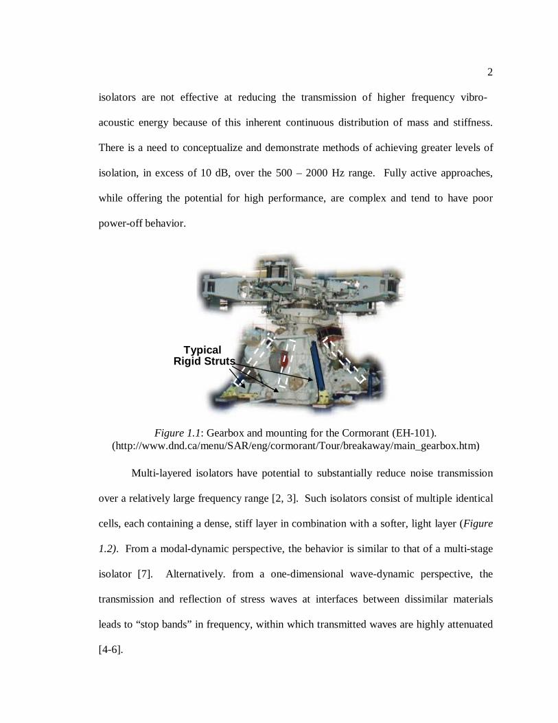
Figure 1.1: Gearbox and mounting for the Cormorant (EH-101).(http://www.dnd.ca/menu/SAR/eng/cormorant/Tour/breakaway/main_gearbox.htm)................................................................................................................2
Figure 1.2: Periodically Layered Isolator in Compression. .......................................3
Figure 1.3: Illustration of Wave Dynamics for frequencies Within and Outside ofStop Band. (http://www.seasalum.ucla.edu/pdf/UEfall02.pdf) ..........................4
Figure 1.4: Lynx Gearbox Noise Identification [12]. ................................................7
Figure 1.5: Growth in Combined Gearbox and Soundproofing Weight at ConstantPower, Constant Design Noise Level [25]. ........................................................10
Figure 1.6: Schematic of ANC Architecture [30]......................................................13
Figure 1.7: Proposed Implementation of Layered Isolators in Gearbox SupportStruts.(http://www.dnd.ca/menu/SAR/eng/cormorant/Tour/breakaway/main_gearbox.htm)................................................................................................................18
Figure 2.1: Comparison of One-Dimensional Transmissibility Predictions forFEM and Floquet Theory for a 3-celled Isolator. ...............................................23
Figure 2.2: First Four Mode Shapes of a Three-celled Isolator in Compression. .......24
Figure 2.3: First Thickness Modes Associated with the Stop Band End FrequencyUsing 1-D and Axisymmetric Models................................................................26
Figure 2.4: Simple Isolator / Mass System in One Dimension. .................................29
Figure 2.5: Simple Isolator / Mass System Modeled with Axisymmetric Elements...29
Figure 2.6: (rS)E vs. Shape Factor. ............................................................................32
Figure 2.7: 1-D /3-D Design Space for (rF)B and (rF)E...............................................33

ix
Figure 2.8: Illustration of Fixed-Free Boundary Condition for a Single Cell. ............37
Figure 2.9: Higher and Lower Approximations for Modes 1 and 2 of a SingleCell. ..................................................................................................................42
Figure 2.10: Experimental Set-up.............................................................................48
Figure 2.11: Experimental and Analytical Transmissibilities for Specimen 1 with4 Cells. ..............................................................................................................50
Figure 2.12: Experimental and Analytical Transmissibilities for Specimen 1 with3 Cells. ..............................................................................................................50
Figure 2.13: Experimental and Analytical Transmissibilities for Specimen 1 with2 Cells. ..............................................................................................................51
Figure 2.14: Experimental and Analytical Transmissibilities for Specimen 1 with1 Cell.................................................................................................................51
Figure 2.15: Experimental and Analytical Transmissibilities for Specimen 2 with4 Cells. ..............................................................................................................52
Figure 2.16: Experimental and Analytical Transmissibilities for Specimen 2 with3 Cells. ..............................................................................................................53
Figure 2.17: Experimental and Analytical Transmissibilities for Specimen 2 with2 Cells. ..............................................................................................................53
Figure 2.18: Experimental and Analytical Transmissibilities for Specimen 2 with1 Cell.................................................................................................................54
Figure 2.19: Comparison of Experimental Transmissibilities for Varying Numberof Cells for Specimen 1. ....................................................................................56
Figure 2.20: Comparison of Experimental Transmissibilities for Varying Numberof Cells for Specimen 2. ....................................................................................57
Figure 2.21: Experimental and Analytical 4-Celled Transmissibilities ofSpecimen 1........................................................................................................58
Figure 2.22: Experimental and Analytical 4-Celled Transmissibilities ofSpecimen 3........................................................................................................58
Figure 3.1: Schematic of Helicopter Transmission Mountings. .................................62
Figure 3.2: 20 year-old layered elastomeric bearing supporting bridge deck inEngland [64]......................................................................................................63

x
Figure 3.3: Schematic of Design Variables...............................................................66
Figure 4.1: Model Schematic of Layered Isolator with Embedded Terfenol-DActuator. ...........................................................................................................77
Figure 4.2: Transmissibility of Three-Layered Isolator with Embedded Terfenol-D Actuator.........................................................................................................80
Figure 4.3: Transmissibility of Isolator with and without Embedded Terfenol-DActuator. ...........................................................................................................81
Figure 4.4: Schematic of Layered Isolator with Embedded Vibration Absorbers. .....82
Figure 4.5: Transmissibility of Example Layered Isolator. .......................................83
Figure 5.1: Schematic of Isolator Configuration with Embedded InertialAmplifiers. ........................................................................................................86
Figure 5.2: Schematic of one inertial amplifier. ........................................................87
Figure 5.3: Mode Shapes at Beginning and End Stop Band Frequencies ofLayered Isolator with Embedded Inertial Amplifiers..........................................89
Figure 5.4: Schematic of Subsystem of Layered Isolator with Embedded InertialAmplifier [54]. ..................................................................................................90
Figure 5.5: Transmissibility of Example Isolator with and without InertialAmplifiers. ........................................................................................................92
Figure 5.6: Axisymmetric Frequency Response Shapes of Example Isolator withEmbedded Amplifiers at Tuned Absorber Frequencies. .....................................93
Figure 5.7: Example Isolator Response Shapes (High Shape Factor, S = 2.6). ..........96
Figure 5.8: Transmissibility and Response Shapes for Layered Isolator withShape Factor = 0.2.............................................................................................98
Figure 5.9: Transmissibility of Low Shape Factor Isolator with and withoutEmbedded Inertial Amplifiers............................................................................99
Figure 5.10: Response Shapes of a Single Layer of the Low Shape FactorExample Isolator with Embedded Inertial Amplifiers: (a) m = 10.6 g, (b) m =5.6 g, (c) m = 3.3 g.............................................................................................101
Figure 5.11: Transmissibility of Example Isolator with and without InertialAmplifiers which Maintain Isolator Periodicity. ................................................103

xi
Figure 5.12: Transmissibility of Stiffened Layered Isolator Example with andwithout Inertial Amplifiers. ...............................................................................105
Figure 5.13: Cut-Away View of a Fluidlastic® Mount [54]......................................106
Figure 6.1: Schematic and Mobility Diagram of Source, Isolator, and Receiver[77]. ..................................................................................................................109
Figure 6.2: Experimental Source and Receiver Mobilities: (a) … Experimental, zdir., - - - Approximation, z dir. (b) …. Experimental, z dir., - - -Approximation, z dir. [23]. ................................................................................112
Figure 6.3: Mobilities of Layered Isolator with Embedded Fluid Elements...............113
Figure 6.4: Analytical Effectiveness of Layered Isolator with Embedded FluidElements. ..........................................................................................................114
Figure 7.1: Transmissibility and Schematic of Single-Celled Specimen toCharacterize Elastomer. .....................................................................................116
Figure 7.2: Single-Layered Specimen with Embedded Fluid Element: (a)Illustration, (b) Cross-section.............................................................................117
Figure 7.3: Analytical and Experimental Transmissibilities of Single-LayeredSpecimen with Embedded Fluid Element...........................................................118
Figure 7.4: Cross-sectional View of Three-celled Specimen with Embedded FluidElements. ..........................................................................................................121
Figure 7.5: Analytical and Experimental Transmissibilities of Three-celledSpecimen to Characterize Elastomer..................................................................123
Figure 7.6: Experimental and Analytical Transmissibility Comparison of OriginalThree-celled Configuration................................................................................124
Figure 7.7: Analytical and Experimental Transmissibilities of Single-celledSpecimen with Embedded Fluid Element...........................................................126
Figure 7.8: Analytical and Experimental Transmissibilities of Two-celledSpecimen with Embedded Fluid Elements. ........................................................128
Figure 7.9: Analytical and Experimental Transmissibilities of Three-celledSpecimen with Embedded Fluid Elements. ........................................................129
Figure 7.10: Experimental Transmissibility Comparison of One, Two, and Three-celled Specimens with Embedded Fluid Elements. ............................................130

xii
Figure 7.11: Transmissibility Comparison of Three-celled Specimen with andwithout Embedded Fluid Elements. ...................................................................131
Figure 7.12: Transmissibilities of Three-Celled Specimen in OriginalConfiguration and Rebuilt Configuration. ..........................................................132
Figure 8.1: Conceptual Configuration for Lower Fluidic Isolator Height. .................140
Figure 8.2: Conceptual Strut Configuration to Ensure Compressive Loads onEmbedded Layered Isolator. ..............................................................................143
Figure 8.3: Conceptual Contractable Inner Diameter Using SMA Wires for Semi-actively Tuning Fluidic Isolators. ......................................................................146
Figure A.1: Geometry of Cylinder ............................................................................162
Figure F.1: Example of Payne Effect for Typical Filled Elastomer [79]. ..................209
Figure F.2: Effect of Dynamic Strain at Room Temperature for Gum and CarbonBlack-Filled Rubber for ε = 0.17, 0.35 0.5, 0.8, 0.88 [80]. .................................210
Figure F.3: Predicted Shear Modulus vs. Frequency at Different Temperatures forTypical Unfilled Elastomer [82]. .......................................................................212
Figure F.4: Modeled Driving Point Stiffness Magnitude and Phase versusFrequency of Sample Isolator for 0% (----), 10% (- - - ), and 20% (- . - .)Precompression at (a) –50 oC, (b)-25 oC, (c) 0 oC, (d) 25 oC, and (e) 50 oC[82]. ..................................................................................................................213
Figure F.5: Unfilled Material Shear Modulus vs. Frequency [79]. ............................215
Figure F.6: Young’s Modulus versus Reduced Frequency for Rubber IsolatorMaterial [83]. ....................................................................................................215
Figure F.7: Stiffness vs. Dynamic Amplitude for Single Frequency andSuperimposed Frequencies for Carbon Black-Filled Isolator [79]. .....................216

LIST OF TABLES
Table 2.1: Shape Factor for Rectangular and Circular Isolators.................................28
Table 2.2: (3-D/1-D) Stiffness Ratios for Different Modes of a 3-celled LayeredIsolator. .............................................................................................................31
Table 2.3: (3-D/1-D) Stiffness Ratios for End Frequency of 3-celled Isolators..........32
Table 2.4: Single Cell Natural Frequencies Using Assumed Modes MethodCompared to 3-D FEM Results..........................................................................40
Table 2.5: Rate of Convergence Comparison for a Single Cell..................................40
Table 2.6: Reduced Powers of ‘r’ and ‘z’ for Ur and Uz to ApproximateBeginning and End Stop Band Frequencies to within 5% Error..........................41
Table 2.7: Summary of Specimen Properties ............................................................49
Table 3.1: Combination of Design Variable and Constraint Values for PassivePerformance Limits of Layered Isolators. ..........................................................69
Table 3.2: Passive Performance Design Runs, Isolator Mass = 2 kg..........................72
Table 3.3: Passive Performance Design Runs, Isolator Mass = 4 kg..........................73
Table 4.1: Optimized Properties of Layered Isolator of Example. .............................82
Table 5.1: Summary of Isolator Eigenvalues with and without Embedded InertialAmplifiers. ........................................................................................................88
Table 5.2: Summary of Example Inertial Amplifier Properties..................................88
Table 5.3: Summary of Inertial Amplifier Properties in Low Shape FactorExample. ...........................................................................................................99
Table 5.4: : Summary of Inertial Amplifier Properties to Maintain IsolatorPeriodicity. ........................................................................................................102
Table 5.5: Summary of Inertial Amplifier Properties in Figure 5.12. ........................105

xiv
Table 7.1: Dimensions of Fluid Elements in Three-layered Specimen.......................122

xv
ACKNOWLEDGMENTS
Foremost, I would like to thank my advisors, Dr. Edward C. Smith and Dr.
George A. Lesieutre, for their encouragement and guidance during my graduate studies at
Penn State. They are both fine educators and superb advisors. In addition, I would like
my committee members, Dr. Kon-Well Wang and Dr. Gary H. Koopmann for their
helpful participation. I would also like to thank all the organizations responsible for
funding this research, including the National Rotorcraft Technology Center, United
Technologies Research Center, and the Lord Corporation, as well as the Vertical Flight
Foundation for their generous scholarship. I especially would like to thank the
individuals at Lord for their indispensable efforts and helpful advice, including Donald
Russell, Scott Redinger, Tejbans Kohli, and Oon Hock Yeoh.

xvi
LIST OF SYMBOLS
[A] Total Constraint matrix
[A1] Dependent constraint matrix
[A2] Independent constraint matrix
a Shorter length of amplified mass lever arm
b Longer length of amplified mass lever arm
bk Coefficients of radial displacement functions
[c] Damping matrix of a single cell
ce Wave propagation speed in elastomer
cw Speed of sound in water
C11, C22, C33, C55,C12, C13, C23 Constitutive material constants
CpT Capacitance of material measured under constant stress
d Isolator diameter
dcell Cell diameter
dk Coefficients of axial displacement functions
dmax Maximum isolator diameter
dmin Minimum isolator diameter
E Isolator effectiveness
Ee Elastomer young’s modulus

xvii
Em Metal young’s modulus
f1 First standing wave frequency of column of water
f1-D General one dimensional isolator natural frequency
f3-D General three dimensional isolator natural frequency
fi Frequency of isolation of fluid-filled isolator
fn1 First natural frequency of single cell
fn2 Second natural frequency of single cell
fB Beginning stop band frequency
fE End stop band frequency
fT Elastomer layer thickness mode natural frequency
fTB Target beginning stop band frequency
fTE Target end stop band frequency
F Force on isolator end
Fa Actuator point force
Fb Base force
Fi Applied input force on isolator
Fy Material yield strength
FO Force on isolator from source side
FR Force on isolator from receiver side
G* Complex shear modulus
Gemax Maximum elastomer shear modulus
Gemin Minimum elastomer shear modulus

xviii
Ge Elastomer shear modulus
Gm Metal shear modulus
Gmmax Maximum metal shear modulus
Gmmin Minimum metal shear modulus
Go Shear modulus at reference temperature
GT Shear modulus at Temperature, T
[G] 3-DOF to 2-DOF transformation matrix
h Layered isolator height
J Quadratic objective function
[k] Stiffness matrix of single cell
k Spring stiffness
k* Effective stiffness of piezoelectric element
kE Effective short circuit material stiffness
k1-D One dimensional isolator stiffness
k3-D Three dimensional isolator stiffness
kA Axial stiffness
kAmax Maximum axial stiffness
kAmin Minimum axial stiffness
keff Effective three dimensional isolator stiffness
kL Lateral stiffness
kLmax Maximum lateral stiffness
kLmin Minimum lateral stiffness
xix
kP Material planar electromechanical coupling coefficient
[K] Stiffness matrix for single cell
[K11], [K22],[K12], [K21] Portions of global stiffness matrix
l Length of general, rectangular isolator
L Length of bound column of water
Lr Cylinder radius
Lz Cylinder half-height
[m] Mass matrix of single cell
m Isolator mass
m1 Mass attached to base pivot of lever arm
m2 Mass attached to top pivot of lever arm
mt Tuned mass at end lever arm
[M] Mass matrix for single cell
M Mobility
M1b Mobility of source-side, with receiver side fixed
M2b Mobility of receiver side, with source side fixed
M1f Mobility of source side, with receiver side free
MI Isolator mobility
MR Receiver mobility
MS Source mobility
[M11], [M22],[M12], [M21] Portions of global stiffness matrix

xx
n Number of cells in layered isolator
{p} Generalized coordinates vector
{P} Total generalized forces vector
{q} Independent coordinates vector
{Q} Transformed independent coordinates vector
r Displacement in radial direction
rF 3-D to 1-D frequency ratio
rS 3-D to 1-D stiffness ratio
R Non-dimensional cylinder radius
R Amplification ratio
S Elastomer shape factor
t General isolator thickness
t11, t12, t21, t22 Components of system transfer matrix
te Elastomer layer thickness
temax Maximum elastomer layer thickness
temin Minimum elastomer layer thickness
tm Metal layer thickness
T Isolator transmissibility
[T] System transfer matrix
u Isolator radial direction
u1 Axial displacement of base pivot of lever arm
u2 Axial displacement of top pivot of lever arm

xxi
ru Evaluated displacement constraint in rth cell
su Evaluated displacement constraint in sth cell
Ur Radial displacement component
Uz Axial displacement component
V Velocity of isolator end
V Volume of cylinder
VO Velocity of source side of isolator
VR Velocity of receiver side of isolator
VRO Velocity of source with massless, rigid connection to receiver
w Width of general, rectangular isolator
w Isolator axial direction
[W1] Penalty weighting matrix for displacement
[W2] Penalty weighting matrix for actuator force
x Displacement of the top metal layer in layered isolator
xb Displacement input at isolator base
xo Baseline displacement of metal layer
xt Transmitted displacement amplitude of isolator
z Displacement in axial direction
Z Non-dimensional cylinder height
α Beginning stop band frequency weighting factor
α Intermediate variable in mobility definitions
α(s) Non-dim. ratio of electrical impedance to electrical impedance

xxii
[β] Constraint transformation matrix
β End stop band frequency weighting factor
χT Empirical shift function
ε1, ε2, ε3, ε5 Strain components in cylindrical coordinates
εrr, εθθ, εzz, εrz Strain components in cylindrical coordinates
φ Empirically derived material property for elastomer
φuj Raidal polynominal displacement functions
φwj Axial polynominal displacement functions
η Complex viscosity
νe Elastomer Poisson’s ratio
νm Metal Poisson’s ratio
θ Angular direction in cylindrical coordinates
λ1 Wavelength of first standing wave in column of water
ρe Elastomer density
ρemax Maximum elastomer density
ρemin Minimum elastomer density
ρm Metal density
ρmmax Maximum metal density
ρmmin Minimum metal density
σι ith stress component in cylindrical coordinates
σc Quasi-static compressive stress

xxiii
σ CDYN Dynamic compressive stress
σrr, σzz, σrz Stress components in cylindrical coordinates
ω Frequency
ωn Natural frequency
( )d Contribution from dependent variables
( )f Contribution from independent variables
( )r Contribution from the rth cell
( )s Contribution from the sth cell
( )c Cosine component
( )s Cosine component

Chapter 1
INTRODUCTION
1.1 Background and Motivation
Dynamic excitations generated by meshing gear pairs is a significant source of
vibration and cabin noise in helicopter transmissions. This high-frequency gearbox noise
is primarily transmitted to the fuselage through rigid connections, which do not
appreciably attenuate vibratory energy (Figure 1.1). The close proximity of the
transmission and cabin in rotorcraft causes interior noise levels that are significantly
higher than those in fixed wing aircraft. The high-frequency vibrations typically include
discrete gear-meshing frequencies in the range of 500 – 4000 Hz, and are often
considered irritating. This high frequency noise can reduce pilot effectiveness and
passenger comfort.
Although elastomeric isolators are frequently used for passive isolation of
mechanical components, these typically operate at relatively low frequencies ( < 100 Hz).
Wave effects occur in conventional isolators at high frequencies when the elasticity and
the distributed mass of the mount interact to create sharp transmissibility peaks [1]. Such
2
isolators are not effective at reducing the transmission of higher frequency vibro-
acoustic energy because of this inherent continuous distribution of mass and stiffness.
There is a need to conceptualize and demonstrate methods of achieving greater levels of
isolation, in excess of 10 dB, over the 500 – 2000 Hz range. Fully active approaches,
while offering the potential for high performance, are complex and tend to have poor
power-off behavior.
Multi-layered isolators have potential to substantially reduce noise transmission
over a relatively large frequency range [2, 3]. Such isolators consist of multiple identical
cells, each containing a dense, stiff layer in combination with a softer, light layer (Figure
1.2). From a modal-dynamic perspective, the behavior is similar to that of a multi-stage
isolator [7]. Alternatively. from a one-dimensional wave-dynamic perspective, the
transmission and reflection of stress waves at interfaces between dissimilar materials
leads to “stop bands” in frequency, within which transmitted waves are highly attenuated
[4-6].
Figure 1.1: Gearbox and mounting for the Cormorant (EH-101).(http://www.dnd.ca/menu/SAR/eng/cormorant/Tour/breakaway/main_gearbox.htm)
TypicalRigid Struts

3
In Figure 1.3, the simple schematic illustrates of the one-dimensional wave
dynamics for frequencies within and outside of the stop band. At frequencies within the
stop band, the waves reflected from the denser material are in phase and act to cancel the
incident wave. As a result, the total transmitted wave is significantly attenuated. At
frequencies outside of the stop band, the reflected waves are out of phase. The total
transmitted wave is therefore not appreciably attenuated.
Another performance benefit of layered isolators is their inherent high axial
stiffness. When the elastomer layers of a layered isolator are compressed quasi-statically,
the actual measured axial stiffness is significantly higher the than one-dimensional
stiffness predicted on the basis of a Young’s modulus. A well-documented method to
account for the difference between the effective three-dimensional stiffness and the
predicted one-dimensional stiffness is the use of a one-dimensional stiffness correction
factor [8 ,9]. Essentially, the shape factor accounts for the discrepancy between the
predicted one-dimensional stiffness and the measured effective one-dimensional stiffness
of an elastomer isolator. Because of this effect, layered isolators can be designed with
Figure 1.2: Periodically Layered Isolator in Compression.
High-FrequencyForce Excitation
Attenuated ForceTransmission
MetalElastomer

4
the high axial stiffness required for helicopter gearbox supports, while also providing
broadband high frequency attenuation. Layered isolators may therefore provide an
elegant solution to the high frequency gearbox noise problem in helicopter cabins.
Figure 1.3: Illustration of Wave Dynamics for frequencies Within and Outside of StopBand. (http://www.seasalum.ucla.edu/pdf/UEfall02.pdf)
Frequencies Within Stop Band
Frequencies Outside of Stop Band
AmplitudeAttenuated
AmplitudeUnattenuated

5
1.2 Literature Review
1.2.1 Sources of High Frequency Noise Inside Helicopter Cabins
Through numerous experimental and analytical studies, the gearbox has been
widely established as the primary source of high frequency noise in rotorcraft cabins.
Pollard has reviewed gearbox noise generation and its transmission via the gearbox and
other airframe structures of the Westland Lynx helicopter [10]. The noise is reported to
be a result of force-fluctuations from the elastic deformation of the gear teeth under load
and tooth manufacturing errors. The fluctuations result in non-uniform gear rotation and
dynamic forces are generated at gear meshing frequencies and harmonics. The forces in
turn excite the gear shafts in torsional, axial, and lateral modes, which cause the bearings
to displace and thus the gearbox casing vibrates and radiates noise. As a result, the
harmonic content of noise radiated to interior microphones is markedly similar to that of
vibrations measured via accelerometers placed on the gearbox casing. Gear meshing
vibrations are directly transmitted to the fuselage because the gearbox is essentially
rigidly mounted to the airframe. Vibration levels of up to 31.6 g at gear meshing
frequencies were measured on the Lynx during flight. Shake tests of the airframe, where
the excitations were applied to the gearbox feet locations, show that the vibration levels
on the airframe were of the same order as the input levels at the gearbox feet. The
vibratory energy is reported to be transmitted to the cabin with little reduction causing

6
individual interior panels to vibrate at large amplitudes and hence radiate noise in the
cabin.
A similar study of the of the Army’s OH-58 helicopter was reported by Coy, et al.
[11]. Flight test data suggest that the planetary gear train is the major source of high
frequency cabin noise. The authors note that it is particularly difficult to block the
structure borne path of interior noise, because the gearbox case and its mounts are an
integral part of the lift-load bearing path. The transmission mounts must be strong
enough to support the entire helicopter by transferring the lift-load from the rotor blades
to the airframe and rigid enough to ensure stable control of the helicopter. Because the
stiff mounts transmit noise exceedingly well, the sound is transmitted to the cabin
directly. Experimental data indicate that the most troublesome noise occurs at the
planetary gear mesh frequency, and thus efforts should be made to attenuate the lowest
frequency gear noise, or 400 – 1000 Hz.
A joint research effort between Aerospatiale and Westland was presented by
D’Ambra and his associates [12]. The authors report that helicopter noise in the audio
range is quite high and exposure time for operations without a protective helmet is
extremely limited. Furthermore, in military helicopters, where available weight for
soundproofing is limited, sound levels obtained after treatment remain in excess of those
desired for reasonable communication. The dominant frequencies composing the cabin
noise resulting from the SA330 Puma gearbox and Lynx gearbox were examined. They
were found to range from 500 – 5000 Hz (Figure 1.4). The researchers note, however,
that the important, acoustically subjective frequencies range from 500 – 2000 Hz.

7
A number of research efforts have focused on predicting helicopter interior noise
levels using Statistical Energy Analysis (SEA) [13-20]. The SEA approach evaluates the
power flow between mechanical structures and/or acoustical spaces. These efforts were
motivated by a need for comprehensive analytic models of the entire aircraft to evaluate
potential noise control measures. One important conclusion should be noted in particular.
Yoerkie, et al., and Morgan, et al., report that using the SEA model, the most efficient
means of reducing noise can be achieved with high frequency vibration isolation between
the gearbox and fuselage [13, 18].
Figure 1.4: Lynx Gearbox Noise Identification [12].

8
Many helicopter transmissions are connected to the fuselage via cylindrical
struts, as in Figure 1.1. Consequently, much research has been devoted to studying the
mechanisms of noise transmission through these support struts. Brennan et al., have
conducted a one-dimensional analysis using the mechanical impedance method, which
allows for the strut to be characterized by two parameters at each end: complex force and
velocity [21]. Both the lateral and longitudinal vibrations through the strut were
examined separately. The longitudinal vibrations are reported to be dominant at low
frequencies, but lateral vibrations become increasingly important at higher frequencies.
Throughout the whole frequency range examined (0 – 10 kHz), however, longitudinal
vibrations appear to have a larger influence on transmitted force than lateral vibrations.
The effectiveness of a 1 mm thick layer of elastomer for vibration isolation was also
examined. The shear stiffness of the elastomeric layer is much lower than the axial
stiffness because of the shape factor stiffness effect. Although it may be possible to
attenuate high frequency flexural vibrations, the authors conclude that a 1 mm thick layer
of elastomer is not an effective isolation treatment for longitudinal vibrations.
Brennan et al. continued this research with an experimental study of the noise
propagation through helicopter support struts [22]. Two simple analytical models of an
EH101 helicopter gearbox strut were first developed. Simulations from the analytical
models were then compared to experimental data, and the main features of the dynamic
behavior of the strut were described with these models. The contributions of
longitudinal, lateral, and torsional vibrations through the strut were ranked based on the
amount of kinetic energy transferred to a receiving structure. The strut was excited so

9
that each of the motions was excited with an equal source strength. The dominant
motion was found to be longitudinal, although lateral and torsional motions were found to
be important at certain flexural resonance frequencies of the strut.
Another analytical and experimental study was performed by Ohlrich using a ¾
scale model of a medium sized helicopter, the BK 117 [23]. In this research effort, the
goal was to determine a suitable source descriptor defined by a set of terminal source
powers which described the strength of the vibrations transmitted from the gearbox to the
fuselage. The source descriptor method is based on the concept of equivalent sources,
which assumes that a vibrating source can be adequately represented by the complex
vibratory power produced by a set of uncorrelated, equivalent point forces. An important
conclusion of this work is that the power transmitted to the fuselage is dominated by axial
vibrations through the struts.
1.2.2 Rotorcraft Interior Noise Control
1.2.2.1 Passive Treatments
A general methodology of helicopter soundproofing was presented by Marze, et
al., which can be applied to aircraft in general [24]. The methodology consists of three
rational steps: diagnosis, design of soundproofing treatments to cabin to obtain desired
noise reductions, and validation and optimization.

10
In general, nearly all helicopter manufacturers have employed this
methodology to apply soundproofing treatments to their aircraft. These approaches,
however, do not attempt to eliminate the noise at its source (gear meshing), nor do they
attempt to acoustically isolate the fuselage from the source of the vibration. Rather,
additional researchers describe add-on soundproofing methods which inherently carry a
considerable weight penalty [16, 24-26]. Marze et al., note that VIP versions of the
Aerospatiale Dauphin helicopter include soundproofing treatments which are 2-3% gross
weight [24]. Owen et al., propose the construction of an inner cabin composed of foam
and lead walls which can impose a weight penalty of 1-3% gross weight of the Westland
Lynx helicopter [26].
Levine notes that as gearbox technology has advanced, the noise generated at a
given horsepower has increased [25]. The result has been that increase in soundproofing
weight has more than offset savings in gearbox weight (see Figure 1.5).
Figure 1.5: Growth in Combined Gearbox and Soundproofing Weight at Constant Power,Constant Design Noise Level [25].
0
500
1000
1500
2000
1960 1970 1980 1990Design Calendar Year
Wei
ght (
lbs)
Gearbox PlusSoundproofing
Gearbox Only

11
Directly quoting Levine: “Main gearbox isolation from the airframe at acoustic
frequencies provides the most weight efficient means of source noise control… This
eliminates the need for heavy soundproofing treatment over large radiating areas. The
added complexity of rotor controls and engine mounting has limited the incorporation of
this approach into helicopter designs to date, but the economics of large-scale helicopter
market penetration will soon force the issue.”
As installed horsepower grows and structural materials become lighter, the
problem of noise increases. To avoid a high weight penalty involved with passive
treatments, many active approaches have been considered and some implemented to
reduce acoustic vibrations / noise.
1.2.2.2 Active Noise Cancellation
An active noise control approach which has received a notable amount of
attention is the use of loudspeakers to cancel sound waves in an enclosure, or active noise
control (ANC) [27-29]. Efforts are made to control cabin noise using a number of
microphones and speakers placed throughout the aircraft cabin. ANC requires no
knowledge of the noise transmission path, but does require in some approaches that the
number of speakers be at least equal to the number of acoustic modes. At higher
frequencies (> 200 Hz), several hundred modes exist at a given frequency [30]. This type

12
of noise control approach is therefore best suited for lower frequencies and becomes
impractical at higher frequencies.
1.2.2.3 Active Structural Vibration Control
Considerable research has focused on developing the active structural acoustic
control (ASAC) approach for interior noise control at frequencies below 500 Hz [31-34,
38]. This approach uses structural actuators and sensors optimally placed on the fuselage
to minimize overall interior noise. As with other active noise control techniques, ASAC
requires a large number of control sources to provide sufficient global sound reduction
over a wide frequency range.
O’Connell, et al., developed two ASAC systems using several small piezoelectric
patches bonded directly to the structure to cancel interior noise of a MD 900 Explorer
helicopter [36]. The authors report tonal noise reductions of 3 to 5 dB in the passenger
cabin with both systems at frequencies up to approximately 1 kHz. A total of 16
actuators and 16 microphones were employed. Fuller, et al., and Sun, et al., investigated
the use of piezoelectric patches to control interior noise in uniform cylindrical shells [37,
38]. A global noise reduction of 10 dB is reported by Fuller, and 20 dB by Sun.

13
1.2.2.4 Minimum Noise Transmission from Gearbox
Much research has been devoted to canceling high frequency vibrations before
they enter the cabin. At Sikorsky, Active Noise Control (ANC, distinct from Active
Noise Cancellation) has proven to be an effective method of actively controlling gearbox
noise [30]. ANC involves a choke-point methodology, where actuators are placed at the
gearbox connection points to the fuselage (Figure 1.6).
When flight tested in a S-76 helicopter, the ANC system reduced the primary
mesh tone (~800 Hz) by 10-20 dB in a variety of flight conditions. The authors also
report that passive choke-point isolation techniques were also investigated at Sikorsky,
such as elastomeric isolators and vibration isolators. Though the elastomeric isolators
showed promise, they raised certification issues since they were placed directly in the
primary load path. Additionally, they would have a significant impact on many aircraft
system design considerations. The tuned dynamic absorbers were ineffective because of
their narrow operating frequency range and limited effectiveness.
Figure 1.6: Schematic of ANC Architecture [30].

14
Many research efforts are focused on actively canceling high frequency
vibrations as they are transmitted through rigid support struts, as in Figure 1.1. The wide
array of active control concepts to control noise through support struts reflects the
importance placed on reducing high frequency vibrations.
In Germany, Eurocopter Deutschland and the EADS research and technology
group have developed the ‘smart strut’ [39, 40]. The smart strut consists of a
conventional BK117 transmission support strut with piezoelectric patches axially bonded
to the exterior. By actively applying shear forces to the strut surface, the control
algorithm attempts to cancel transmitted high frequency noise. The authors report that an
11 dB reduction at gear-meshing frequency of 1900 Hz was achieved for forward flight
of 60 kt. Other gear meshing frequencies, however, were unattenuated. The high noise
reduction is not attainable for all flight conditions, however. As forward flight speed
increases, the active system becomes less effective. This performance degradation is
reported to be caused by limited actuator performance with increasing vibration levels.
Current work is focused on improving actuator performance via optimized actuator
design.
In England, researchers at the Institute of Sound and Vibration Research at the
university of Southhampton, and researchers at Westland Helicopters, have characterized
the strut transmission problem and have attempted to develop active control strategies
[41]. An EH101 support strut was set up in the laboratory under realistic loading
conditions and three magnetostrictive actuators were clamped around its circumference at
a certain length along the strut. The purpose of the actuators was to introduce secondary

15
vibration in the frequency range of 250 – 1250 Hz to minimize the kinetic energy of
vibration of the receiving structure. This attenuation was calculated with knowledge of
measured frequency response data of the strut and actuators. A calculated attenuation of
around 40 dB in the kinetic energy was experimentally observed at some discrete
frequencies, which did not necessarily correspond to gear meshing frequencies. The
control system was found to be practical at frequencies up to at least 1250 Hz. The
authors concede, however, that two endplate masses supporting the strut strongly affected
the dynamic response of the complete experimental assembly, and that boundary
conditions experienced by a strut under flight conditions would be completely different.
At the University of Maryland, Balachandran, Pelinescu, et al., have investigated
both longitudinal and flexural wave transmission through support struts and active
control strategies, as well [42-48]. The control configuration consists of either a
magnetostrictive actuator or piezoelectric stack attached to the end of a support strut, or
in some cases, clamped at an angle along the length of the strut. Reaction mass is
included in both actuator configurations. For harmonic longitudinal disturbances, an
experimental reduction of up to 30 dB of the transmitted disturbance through the strut
was achieved using two different piezoelectric configurations, whereas only up to 16 dB
reduction was achieved using one magnetostrictive actuator. Current and future work is
focusing on digital implementation of a closed loop control algorithm. The authors note,
however, that in a practical situation, availability of required electrical power, actuator
and sensor bandwidths, and actuator heating effects are major constraints.

16
1.2.3 Periodically Layered Media for High Frequency Isolation
In 1986, Sackman and his associates reported that periodically-layered metallic
and elastomeric shear mountings are potential attenuators of dynamic stresses at high
frequencies [5, 6]. The impedance difference between layers is the attenuation
mechanism, in which an incident wave is scattered and essentially split into a reflected
and refracted wave. The device becomes increasingly effective with a larger impedance
mismatch between the isolator materials.
A one-dimensional analysis of periodically-layered isolators in compression
(Figure 1.1) was presented by Ghosh in 1985 [4]. Motivation for the research effort was
isolation of reactor components and structures from seismic, impact, or other accident-
induced loads. A time-domain solution was obtained for plane stress excitation through
layered composites, which makes use of continuity of stress and displacement at the layer
interfaces. Plane longitudinal stress waves are attenuated in periodically-layered elastic
mounts, whereas no attenuation is exhibited by an undamped homogeneous elastic
medium.
A one-dimensional analysis of layered isolators, based on the theory of shear
waves in infinite, periodically layered media is presented by Sackman, et al. [4, 5].
Floquet theory was used to solve the equations for the propagation of plane waves
through a laminated system of parallel plates. The direction of propagation is normal to
the plates, which are composed of one of two materials. The theory predicts high
frequency “stop bands” within which vibratory energy is attenuated. The analysis
includes a method for predicting the beginning and end frequencies of stop bands. Thus,

17
the layered isolator behaves in some sense as a mechanical notch filter. The existence
of the predicted stop bands was corroborated by testing of layered specimens in shear.
The test specimens were of finite length, and therefore edge effects and reflections from
the top and bottom layers were observed in the experiment. These effects, however, did
not obscure the basic physical phenomenon of stop bands.
The phenomenon of transmissibility stop bands occurring in periodic structures
has been known for over a century. Around the turn of the century, Lord Kelvin
proposed a “mechanical filter” to filter out vibrations at certain frequencies, which was
later experimentally validated by Vincent [49]. The filter consisted of discrete masses
connected by springs. The research efforts of Sackman, et al., and Ghosh are highlighted
because of their focus on elastomer and metal composites.
1.3 Research Objectives
The overall objective of the subject research effort was to develop new concepts
and design methods for periodically layered metal and elastomer isolators in
compression. To accomplish this objective, the three-dimensional elastic behavior of
layered isolators was investigated using both analytical simulation and experimental
testing. The next goal was to evaluate the feasibility of using layered isolators to reduce
noise and vibration transmitted into helicopter cabins by meshing transmission gears. A
major supposition of the research effort is that a choke-point vibration control
methodology can be employed, wherein all flight loads are transmitted through layered

18
elastomeric and metal isolators before they enter the cabin, as pictured in Figure 1.7.
The approach taken to reach these objectives was as follows:
1) An analytical method was developed to accurately predict isolator stop band
beginning and end frequencies. The method accurately captures the axisymmetric elastic
behavior of vibrating cylinders and accommodates varying geometry, elastomer shape
factor, and number of cells. In addition, the method calculates transmissibility as a
function of frequency.
2) Extensive experimental testing of layered specimens was performed to validate
the analysis method. Experimental and analytical transmissibilities of layered test
specimens having the identical elastomer, but different shape factors and different
numbers of cells were compared. The experimental and analytical transmissibilities of
geometrically-similar test specimens with differing elastomeric damping were also
compared.
Figure 1.7: Proposed Implementation of Layered Isolators in Gearbox Support Struts.(http://www.dnd.ca/menu/SAR/eng/cormorant/Tour/breakaway/main_gearbox.htm)
LayeredIsolators
Embedded inSupport Struts

19
3) The design constraints associated with the proposed gearbox high-frequency
isolator were determined. Important issues investigated included isolator mass, stiffness,
fatigue and geometry.
4) A design optimization methodology was developed to evaluate the passive
performance limits of periodically layered isolators to isolate helicopter gearboxes. The
design optimization methodology was evaluated using different combinations of design
constraints, such as restricted mass, axial stiffnesses and geometries.
5) As a result of passive performance limitations of layered isolators, design
enhancements were considered to improve isolator performance to meet isolation
objectives of the gearbox noise problem. Active, semi-active, and passive design
enhancements were all investigated to improve performance and tunability. A passive
enhancement in the form of embedded inertial amplifers was pursued and experimentally
validated.
6) A final step was the development of guidelines and computational tools for
gearbox isolator design to accommodate a variety of helicopter sizes and transmission
configurations. If layered composites prove feasible and attractive as gearbox isolators,
designers will need tools to begin practical evaluations.

20
The use of layered isolators as high frequency gearbox isolators would be a
new and novel approach. Although layered isolators in shear have been investigated in
the literature, layered elastomeric and metal isolators in compression have not been
modeled in any great detail. An axisymmetric approximation method allows for accurate
prediction of layered isolator stop band frequencies in compression. The design of
layered isolators in compression would allow for relatively high isolator quasi-static
stiffness, while ensuring low isolator stiffness over certain predicted stop band frequency
ranges. To provide tunability and improve performance, active, semi-active, and passive
enhancements to layered isolators were investigated. These efforts will yield new
insights into the state-of-the-art of high frequency isolation.

Chapter 2
PERIODICALLY LAYERED ISOLATORS FOR HIGH FREQUENCY
ISOLATION
Periodically layered elastomer and metal composites in shear are known to exhibit
high frequency stop bands in which transmitted vibrations are significantly attenuated [4,
5]. The utility of employing these isolators in compression was investigated, and an
analysis method was developed to predict their high frequency behavior. Finally, a series
of experiments were conducted to validate the analysis.
2.1 One Dimensional Finite Elements Analysis
A one-dimensional finite element analysis of layered isolators was developed for
comparison with the analytical method presented by Sackman, et al. [4, 5], who used
Floquet theory to predict high frequency stop bands. The beginning and end stop band
frequencies are referred to as fB and fE, respectively. Each layer of the layered isolators
was modeled using two-noded axial finite elements. Using the discretized equations of

22
motion, a frequency domain analysis was performed to determine transmissibility of the
multi-layered isolator.
As an example, consider an isolator with 3 steel and elastomer cells, and a cross-
sectional area of 5 cm2, in which both the steel and elastomer layers had a thickness of 1
cm. The material properties were Ee=5MPa, Em = 200 GPa, ρe = 1,000 kg/m3 and
ρm=7,800 kg/m3. The solution converged when each elastomer layer was modeled with
10 elements, and each steel layer with 3 elements. The transmissibility predictions from
both finite element analysis and Floquet theory are presented in Figure 2.1. Both
transmissibility results are identical within the stop band frequency range. Isolator
transmissibility is defined as the transmitted displacement amplitude, xt, divided by the
base input amplitude, xb, and can be written as
( )
( )t
b
xT
x
ωω
= ( 2.1 )
Three discrete isolator resonance peaks are evident from the finite element analysis,
which are not predicted in the analyses in [4] and [5].
This one-dimensional finite element analysis provided a clearer understanding of
layered isolator behavior in shear, but a more detailed finite element analysis needed to
be performed to better understand the three-dimensional behavior of layered isolators in
compression.

23
2.2 Three Dimensional Finite Element Analysis
A detailed finite element analysis of periodically layered isolators was conducted
to gain an improved understanding of three-dimensional effects on isolator performance
[1]. Mode shapes and isolator transmissibility were examined. Parabolic quadrilateral
axisymmetric elements were used to model each layer of the circular isolator [50]. Each
element had eight nodes and forty-eight degrees of freedom. All deflections and rotations
were constrained at the base of the isolator. Transmissibility was calculated in the
frequency domain by dividing the total axial reaction force (obtained using equilibrium
equations), Fb, by the total applied input force at the top of the unconstrained isolator
surface, Fi, and can be written as
Figure 2.1: Comparison of One-Dimensional Transmissibility Predictions for FEM andFloquet Theory for a 3-celled Isolator.
1.E-04
1.E-03
1.E-02
1.E-01
1.E+00
1.E+01
1.E+02
1.E+03
0 1000 2000 3000 4000Frequency (Hz)
Tra
nsm
issi
bili
ty
1D FEM
FloquetTheory
Stop Band
fB fE
IsolatorResonance

24
b
i
FT
F= ( 2.2 )
For a typical three-celled isolator, the first four mode shapes are illustrated in Figure 2.2.
For the first n modes, each elastomer layer associated with these frequencies
undergoes approximately uniform axial strain. In fact, the metal layers behave essentially
like discrete masses supported by n axial springs. Invariably, the first mode shows that in
each elastomer layer the strain is either all compression or all tension. In the next (n-1)
modes, the mode shapes of the individual layers are observed to contain different
combinations of layerwise compression and tension. The (n+1)th mode (mode 4 in
Figure 2.2) is the first mode in which each elastomer layer exhibits a ‘thickness’ mode.
Figure 2.2: First Four Mode Shapes of a Three-celled Isolator in Compression.
Mode 1 Mode 2 Mode 3 Mode 4
nth Mode (n+1)th Mode
Stop Band

25
Physically, this mode involves both tension and compression within the elastomer layer
and minimal net axial motion of the constraining metal layers. This mode is associated
with the end of the stop band frequency range.
The mode associated with the end frequency warrants closer examination.
Referencing Sackman’s analysis, z is the ratio of the input frequency to the natural
frequency of the first thickness mode. The thickness mode can be closely approximated
as the first mode under the condition that both ends of a single elastomer layer are
constrained. In the one-dimensional analysis, the natural frequency associated with the
first thickness mode of an elastomer layer, fT, also marks the end of the stop band, fE, and
is expressed as
2e
T Ee
cf f
t= = ( 2.3 )
where ce is the axial wave speed through the elastomer layer, and te is the elastomer layer
thickness. For a given isolator, the end frequency is then associated with the first
thickness mode of a single elastomer layer.
The one-dimensional and axisymmetric thickness modes for a single elastomer
layer are illustrated in Figure 2.3. Note, the one-dimensional model allows only axial
motion, whereas the axisymmetric model captures pronounced lateral motion, as well as
axial motion. Therefore, a discrepancy is expected between the natural frequency
predictions of the two models.

26
A design analysis for layered isolators requires accurate prediction of the highest
isolator natural frequency in which all layers exhibit uniform axial strain. Additionally,
the natural frequency associated with the first thickness mode of a single elastomer layer
must also be accurately predicted.
2.2.1 One Dimensional Stiffness Correction Factors
The first three modes in Figure 2.2 show the significant lateral motion of the
middle of each elastomer layer. This is due to fact that the upper and lower surfaces of
each layer are constrained and that elastomers are nearly incompressible. Consequently,
the effective three-dimensional stiffness of each layer is expected to differ from the
predicted one-dimensional stiffness, which only addresses axial motion.
A well-documented method to account for the difference between the effective
three-dimensional stiffness and the predicted one-dimensional stiffness is the use of a
one-dimensional stiffness correction factor, or shape factor. Essentially, the shape factor
accounts for the discrepancy between the predicted one-dimensional stiffness and the
Figure 2.3: First Thickness Modes Associated with the Stop Band End Frequency Using1-D and Axisymmetric Models.
One Dimension Axisymmetric
d/2 d/2
Tension
Compression
zz

27
measured effective one-dimensional stiffness of an elastomer isolator. Shape factor is
defined as the ratio of one bonded area to the force-free area of an elastomer isolator.
Expressions for shape factor for different geometries have been formulated both
empirically, and analytically [7, 8]. The total displacement of a bonded isolator can be
considered to arise from a superposition of two displacements [7]: (a) those caused by the
same deformation of an unbonded isolator (between frictionless rigid surfaces), and (b)
the shear displacements necessary to restore points in the bonded planes to their original
position. Gent and his co-authors provide a comprehensive discussion [7].
The one-dimensional quasi-static stiffness of a single elastomer layer, without
including bonding shear effects, is given as
1e e
De
E Ak
t− = ( 2.4 )
where Ee is the Young’s modulus, Ae is cross-sectional area, and te is the elastomer
thickness. To simplify the design of isolators, the one-dimensional stiffness is multiplied
by an empirically determined function of the shape factor to approximate the effective
isolator stiffness. This is illustrated in table 1 for rectangular and circular isolators.

28
The effective stiffness is then given as
21 (1 2 )eff Dk k Sφ−= + ( 2.5 )
where S is the shape factor, and φ is an empirically derived factor to account for
experimental deviations in the behavior of different elastomers [8]. To simplify the
discussion, it is assumed φ = 1.
The shape factor is used for the design of elastomeric mounts for low frequency
isolation. For a simple one-dimensional isolator / mass system shown in Figure 2.4,
where d is isolator diameter, the first natural frequency can be predicted with
eff
n
k
Mω = ( 2.6 )
Table 2.1: Shape Factor for Rectangular and Circular Isolators
d
t
w
l
t 2 2 2 ( )
lw lwS
tw tl t l w= =
+ +
2
44
dd
Sdt t
π
π= =

29
For the same system, Figure 2.5 shows the axisymmetric mode shape associated
with this natural frequency. This mode shape was determined using axisymmetric
elements [50].
Recalling Figure 2.2, this mode shape is similar to the shapes exhibited by the
individual elastomer layers for the first n isolator natural frequencies of an n-celled
isolator. The nth natural frequency is the beginning frequency. For the one dimensional
analysis, it would therefore appear that applying the shape factor to each layer of the
isolator is appropriate for predicting the first n natural frequencies in three-dimensions.
Figure 2.4: Simple Isolator / Mass System in One Dimension.
Figure 2.5: Simple Isolator / Mass System Modeled with Axisymmetric Elements.
keff
Mωn
d
M
z
ωn
d/2

30
2.2.1.1 Shape Factor Influence on Higher Modes
To investigate the validity of this assumption, a typical three-celled layered
isolator with a shape factor equal to 1 was modeled using axisymmetric elements [50].
The isolator had the following properties: n=3, d = 10 cm, Ee = 15 MPa, Em = 200 GPa,
ρe=1,000 kg/m3, ρm = 7,800 kg/m3, te=2.5 cm, and tm=1.0 cm.
The elastomer layers were each modeled with five parabolic quadrilateral
elements across te, and five elements across d/2. The steel layers were modeled with 1
element across tm, and five elements across d/2.
The first 5 natural frequencies were then compared to the natural frequencies
resulting from a one-dimensional analysis. A 3-D to 1-D stiffness ratio, rS, was then
calculated using the formula
223 3
2
1 1
D DF
D D
S
k fr r
k f− −
− −
= = = ( 2.7 )
where rF is the 3-D to 1-D frequency ratio. Table 2.2 shows the isolator properties and
results. As expected, the ratio for the first mode is approximately equal to 3. The ratios
for subsequent natural frequencies show a decreasing trend. The third mode, associated
with the beginning frequency, shows a ratio of 1.93. The decreasing ratio values suggest
that the quasi-static shape factor cannot be directly utilized for accurate prediction of the
nth isolator natural frequency, or the beginning frequency.

31
A similar investigation was also performed for the stiffness ratio of the (n+1)th
isolator natural frequency, or the end frequency. This natural frequency was calculated
using both axisymmetric FEM and the one-dimensional prediction method for different
elastomer layer geometries, or different shape factors. The isolator had the same
properties as the previous investigation, except for te, which varied to account for
different shape factors.
Table 2.3 shows the stiffness ratios for the different cases. As expected, the
smaller the shape factor, the closer the stiffness ratio comes to unity. As shape factor
increases, however, the stiffness ratio decreases. These trends are illustrated in Figure
2.6.
Table 2.2: (3-D/1-D) Stiffness Ratios for Different Modes of a 3-celled Layered Isolator.
1 177 306 2.992 506 786 2.41
1 3 3 747 1037 1.934 2493 2409 0.935 2596 2412 0.866 2713 2415 0.79
ShapeFactor
(1+2S2) Mode 3-D fn.1-D fn rS

32
Table 2.3: (3-D/1-D) Stiffness Ratios for End Frequency of 3-celled Isolators.
Figure 2.6: (rS)E vs. Shape Factor.
0.5 1224 1320.7 1.16 0.75 1839 2002 1.19 1 2449 2652 1.17 2 4899 5180 1.12 3 7351 7334 1.00 4 9798 9407 0.92 5 12247 11329 0.86 6 14685 13235 0.81 7 17153 15169 0.78 8 19596 17092 0.76
(rS)EShapeFactor 1-D 3-D(Hz) (Hz)
0.6
0.7
0.8
0.9
1.0
1.1
1.2
1.3
0 1 2 3 4 5 6 7 8 9Shape Factor
rE(rS)E

33
2.2.2 Table Look-up Methodology
A preliminary method was developed to accurately predict beginning and end
frequencies in three dimensions. This was accomplished by mapping out a design space
with the following discrete design variables: shape factor, S, number of layers, n, and
isolator diameter, d. This forms a three-dimensional design space that is illustrated
graphically in Figure 2.7. A look-up method approach was used so that computationally
expensive axisymmetric finite element modeling could be avoided in future design
optimization routines.
For given isolator properties, each ‘node’ in this space contains the 3-D to 1-D
frequency ratios for both the beginning and end frequencies, expressed as
( ) 3
1
D
F B
D B
fr
f
−
−
=� �� �� �
, ( ) 3
1
D
F E
D E
fr
f
−
−
=� �� �� �
( 2.8 )
Figure 2.7: 1-D /3-D Design Space for (rF)B and (rF)E.
12
34 2 4 6 8
5 cm
10 cm
20 cm
34
56
78
Dia
met
erLay
ers
Shape Factor

34
The 1-D frequencies are calculated using the method described in [5] and [6], and
the 3-D frequencies were calculated using axisymmetric elements [50]. Based on 1-D
calculations, the 3-D modal behavior is then linearly interpolated.
To accurately capture axisymmetric behavior, however, this approach requires
numerous axisymmetric FEM solutions for the entire design space of possible isolator
geometries. A more elegant method to predict isolator behavior was therefore pursued.
2.3 Axisymmetric Approximation Method
A more accurate and general method was developed for predicting the
axisymmetric behavior of layered isolators and is summarized here [2]. The method
combines a Ritz approximation method with a component mode synthesis technique. For
given isolator geometry, material properties, and number of cells, the axisymmetric stop
band frequencies and the frequency-dependent transmissibility are calculated.
2.3.1 Natural Frequency of 3-D Cylinders of Finite Length
A closed-form solution for natural modes of a vibrating cylinder is
mathematically very difficult to obtain. Thus, several approximation methods have been
pursued. Heyliger presents a technique for calculating the natural frequencies of the
axisymmetric vibrations of anisotropic and isotropic cylinders of finite length [51]. This

35
method is general and can be applied to cylinders having a variety of boundary conditions
and material properties.
The displacement components that describe the axisymmetric motion of an elastic
cylinder can be expressed as
( , )ru U r z= , ( , )zw U r z= ( 2.9 )
where u and w are independent displacements in the radial and axial directions,
respectively. The strain components for axisymmetric motion can be written in
cylindrical coordinates as
,1 r
urr ∂
∂== εε 2 ,u
rθθε ε= = ,3 z
wzz ∂
∂== εε z
u
r
wrz ∂
∂+∂∂== εε5 ( 2.10 )
The reader is referred to Heyliger’s analysis for a detailed derivation of the
equations of motion and possible boundary conditions [51]. A summary of the derivation
is presented in Appendix A for completeness. Analytical solutions to the equations of
motion are difficult to obtain, and thus approximate solutions for the governing equations
of motion are constructed by using the assumed modes method, in which u and w are
approximated by finite linear combinations of the form
1
( , ) ( , )N
uk k
k
u r z b r zφ=
=� , 1
( , ) ( , )M
wk k
k
w r z d r zφ=
=� ( 2.11 )
Here φuk and φw
k are known functions of position, n represents the number of terms for
the displacement components, and bk and dk are constants.
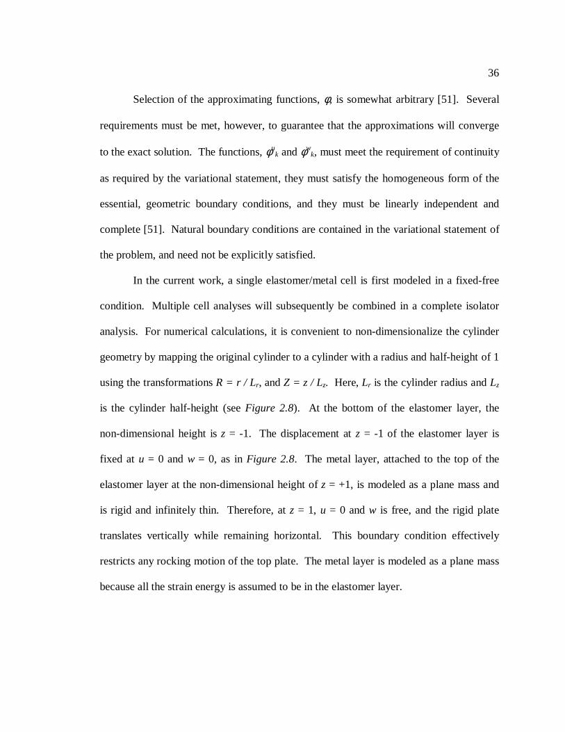
36
Selection of the approximating functions, φ, is somewhat arbitrary [51]. Several
requirements must be met, however, to guarantee that the approximations will converge
to the exact solution. The functions, φuk and φw
k, must meet the requirement of continuity
as required by the variational statement, they must satisfy the homogeneous form of the
essential, geometric boundary conditions, and they must be linearly independent and
complete [51]. Natural boundary conditions are contained in the variational statement of
the problem, and need not be explicitly satisfied.
In the current work, a single elastomer/metal cell is first modeled in a fixed-free
condition. Multiple cell analyses will subsequently be combined in a complete isolator
analysis. For numerical calculations, it is convenient to non-dimensionalize the cylinder
geometry by mapping the original cylinder to a cylinder with a radius and half-height of 1
using the transformations R = r / Lr, and Z = z / Lz. Here, Lr is the cylinder radius and Lz
is the cylinder half-height (see Figure 2.8). At the bottom of the elastomer layer, the
non-dimensional height is z = -1. The displacement at z = -1 of the elastomer layer is
fixed at u = 0 and w = 0, as in Figure 2.8. The metal layer, attached to the top of the
elastomer layer at the non-dimensional height of z = +1, is modeled as a plane mass and
is rigid and infinitely thin. Therefore, at z = 1, u = 0 and w is free, and the rigid plate
translates vertically while remaining horizontal. This boundary condition effectively
restricts any rocking motion of the top plate. The metal layer is modeled as a plane mass
because all the strain energy is assumed to be in the elastomer layer.

37
Several different sets of functions could be selected to obtain an approximate
solution. In this work, they must satisfy the boundary conditions u = 0, w = 0 at z = -1,
and imposed conditions u = 0, w unconstrained and uniform at z = 1. A series of
approximating functions were developed that consist of power series in the r and z
directions and satisfy the preceding conditions. The functions for the radial direction can
be summarized as
1 0
( , ) ( 1)( 1)n m
u i jk
i j
r z r z z zφ= =
= + −�� , 1..[ ( 1)]k n m= × + ( 2.12 )
where n and m are chosen to vary the maximum power of variables, ‘r’ and ‘z’. All
approximating functions in the u direction must include an ‘r’ term because they describe
an axisymmetric displacement. In the axial direction the functions are formed slightly
differently,
1 ( 1),w zφ = + 0 0
( , ) ( 1)( 1) ( 1)s t
w i jk
i j
r z r z z z zφ= =
� �= + − + +� ��� ,
2..[( 1) ( 1)]k s t= + × +
( 2.13 )
Figure 2.8: Illustration of Fixed-Free Boundary Condition for a Single Cell.
r
z
z = -1
z = +1
r = 1r = 0
z = 0
Rigid, Thin MetalLayer

38
where again, s and t are chosen to vary the maximum power of variables ‘r’ and ‘z’ . All
terms for the w direction need not include an ‘r’ term. However, any term multiplied by
‘r’ is forced to zero at z = +1 to satisfy the imposed boundary condition of uniform axial
displacement of the top plate. Alternatively, the displacement in the w direction can only
have a radial dependence from –1 < z < +1. Substitution of approximation functions in
Equation 2.11 into the weak form of the governing equations yields an eigenvalue
problem of the form
[ ] [ ]( )2 { } {0}K M pρω− = ( 2.14 )
The vector {p} contains the coefficients b and d from Equation 2.11 which correspond to
different cylinder mode shapes. The explicit forms of matrices [M] and [K] in terms of φu
and φw are reported by Heyliger [51], and can be found in Appendix B.
2.3.2 Numerical Results for a Single Cell
Numerical simulations were performed for a single cell to compare the natural
frequency predictions using the Ritz method to axisymmetric finite element results. The
first and second modes were examined, because these modes are the component mode
shapes important to the nth and (n+1)th isolator modes, respectively. An n-celled isolator
is illustrated in Figure 2.2. The boundary conditions were fixed-free, as illustrated in
Figure 2.8. The general material properties used were: Gm = 100 Pa, νm = 0.3, ρm = 10
39
kg/m2, Ge = 1 Pa, νe = 0.5, ρe = 1 kg/m3, te = 1 m, and dcell = 1 m. Note that the units for
ρmetal are mass per unit area, as appropriate for a vanishingly-thin metal layer.
The axisymmetric finite element model consisted of parabolic quadrilateral
axisymmetric elements, with 20 elements across the radius, and 20 elements through the
thickness of the elastomer layer. The strain in the metal layer is insignificant, and thus
only 5 elements are used across its thickness. This number of elements was found to be
sufficient for convergence over the frequency range of interest. The frequencies
calculated using the finite element analysis were
fn1 = 0.094 Hz
fn2 = 0.917 Hz
These values are used in subsequent comparisons to the Ritz predictions as baseline
cases. Note that the material properties and isolator dimensions are arbitrary for this
case, so that these frequencies do not have a physical significance related to layered
isolators. This case is only used to validate the mathematics of the linear approximation
method.
The first and second natural frequencies calculated with the Ritz method are
presented in Table 2.4. A percent error is also calculated with reference to the
axisymmetric finite element predictions. Combinations of the powers of the ‘r’ and ‘z’
polynomials are used in the approximating functions for both Ur and Uz. To simplify the
tabular results, the power of ‘r’ in both the Ur and Uz approximating functions is the same
for a given result. Similarly, the power of ‘z’ is the same in both the radial and vertical
approximating functions. As can be observed from Equation 2.12, the lowest possible

40
power of ‘z’ in the radial direction is 2. This is therefore the lowest power used for both
directions.
As seen in Table 2.4, as the powers of ‘r’ and ‘z’ increase, the Ritz predictions
appear to converge to the axisymmetric finite element results. Table 2.5 lists the rates of
convergence for both methods. The first and second natural frequencies of a single cell
are computed for different number degrees of freedom in the elastomer layer. The Ritz
method is observed to be significantly more accurate per degree of freedom.
Table 2.4: Single Cell Natural Frequencies Using Assumed Modes Method Compared to3-D FEM Results.
Table 2.5: Rate of Convergence Comparison for a Single Cell.
zp p 2 3 4 5
(Hz) % Error (Hz) % Error (Hz) % Error (Hz) % Errorrq q
fn1 0.4594 388 0.0983 4.5 0.0982 4.4 0.0959 2.01
fn2 11.2542 1128 5.6200 513 0.9745 6.3 0.9744 6.3
fn1 0.4594 388 0.0982 4.5 0.0981 4.4 0.0951 1.22
fn2 11.2542 1128 5.4220 491 0.9379 2.3 0.9377 2.3
fn1 0.4594 388 0.0982 4.5 0.0981 4.3 0.0950 1.13
fn2 11.2472 1127 5.4211 491 0.9338 1.9 0.9335 1.8
Ritz Method Axisymmetric FEMTotal DOF fn1 (Hz) fn2 (Hz) Total DOF fn1 (Hz) fn2 (Hz)
3 0.4594 11.254 10 0.4576 6.76110 0.0983 5.6200 32 0.1041 4.06821 0.0981 0.9379 66 0.1002 1.00536 0.0950 0.9335 170 0.0967 0.953655 0.0943 0.9179 640 0.0948 0.926978 0.0942 0.9177 2480 0.0940 0.9168
Approximation Method
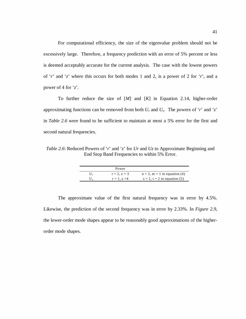
41
For computational efficiency, the size of the eigenvalue problem should not be
excessively large. Therefore, a frequency prediction with an error of 5% percent or less
is deemed acceptably accurate for the current analysis. The case with the lowest powers
of ‘r’ and ‘z’ where this occurs for both modes 1 and 2, is a power of 2 for ‘r’, and a
power of 4 for ‘z’.
To further reduce the size of [M] and [K] in Equation 2.14, higher-order
approximating functions can be removed from both Ur and Uz. The powers of ‘r’ and ‘z’
in Table 2.6 were found to be sufficient to maintain at most a 5% error for the first and
second natural frequencies.
The approximate value of the first natural frequency was in error by 4.5%.
Likewise, the prediction of the second frequency was in error by 2.33%. In Figure 2.9,
the lower-order mode shapes appear to be reasonably good approximations of the higher-
order mode shapes.
Table 2.6: Reduced Powers of ‘r’ and ‘z’ for Ur and Uz to Approximate Beginning andEnd Stop Band Frequencies to within 5% Error.
Power
Ur r = 2, z = 3 n = 2, m = 1 in equation (4)Uz r = 1, z =4 s = 1, t = 2 in equation (5)

42
2.3.3 Analysis of Layered Isolators Using Component Mode Method
A method was developed by Hurty for analyzing complex structures that can be
divided into interconnected components [52]. For this work, a single component is
considered to be a combination of an elastomer and metal layer, or a cell in a periodically
layered isolator. All strain is considered to be in the elastomer portion of the cell.
Displacements of each cell are expressed in terms of generalized coordinates, {p}, and
are defined by assumed displacement modes [51]. In this work, the assumed modes take
the form of Equations. 2.12 and 2.13 and include a rigid body mode in the z direction
with constant displacement. This mode allows for rigid body motion of cells when
interconnected.
When continuity conditions are imposed at cell boundaries, a set of constraint
equations results which expresses kinematic relationships among the coordinates
Figure 2.9: Higher and Lower Approximations for Modes 1 and 2 of a Single Cell.
Mode 1 Mode 2 Mode 1 Mode 2
Higher Order Lower Order
UrPower of ‘r’: 3Power of ‘z’: 5 Uz
Power of ‘r’: 3Power of ‘z’: 5 Ur
Power of ‘r’: 2Power of ‘z’: 3 Uz
Power of ‘r’: 1Power of ‘z’: 4

43
associated with different cells [52]. These constraint equations are used to determine a
set of overall system (isolator) generalized coordinates equal to the total number of cell
coordinates minus the number of constraint equations. The relationship between the sets
of cell generalized coordinates and the set of isolator generalized coordinates is expressed
in the transformation matrix, [β]. Isolator mass, stiffness, and damping matrices are
obtained through this transformation. Forces on component cells are also transformed
into total system forces in this way. A set of equations of motion for the entire isolator
results.
The procedure used to obtain isolator equations of motion, as presented by Hurty
[52], is summarized here. The equation of motion for the sth cell of the isolator can be
expressed as
[ ] { } [ ] { } [ ] { } { ( )}s s s s s s sm p c p k p P t+ + =�� � ( 2.15 )
where
{ } ,{ } ,{ }s s sp p p� �� = column vectors of cell generalized displacements, velocities, and
accelerations
[ ] ,[ ] ,[ ]s s sm c k = square matrices of cell generalized masses, damping, and stiffnesses.
{ ( )}sP t = column vector of generalized forces applied to the sth cell. These
include forces transmitted through constraints as well as externally
applied forces [52].

44
Using Equation 2.15, equations are written for all isolator cells. The sets of cell
equations of motion are grouped together in matrix form to create a total isolator set of
equations:
[ ]{ } [ ]{ } [ ]{ } { ( )}m p c p k p P t+ + =�� � ( 2.16 )
When forming [m], [c], and [k], it is desirable to group cell generalized coordinates
together, as in
1
2
{ }{ }
.
.{ }
{ }{ }
.
.
r
s
pp
ppp
� �� �� �� �� �= � �� �� �� �� �� �
,
1
2
{ }( ){ }( )
.
.{ ( )}
{ }( ){ }( )
.
.
r
s
P tP t
P tP tP t
� �� �� �� �� �= � �� �� �� �� �� �
( 2.17 )
Grouped in this way, the mass matrix takes the form
1
2
[ ] . . . . . . 0. [ ] .. .. . .
[ ]. [ ] .. [ ] .. . .0 . . . . . . .
r
s
mm
mm
m
� �� �� �� �� �=� �� �� �� �� �� �
( 2.18 )
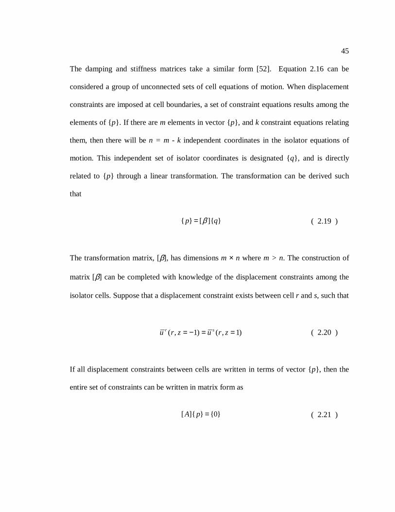
45
The damping and stiffness matrices take a similar form [52]. Equation 2.16 can be
considered a group of unconnected sets of cell equations of motion. When displacement
constraints are imposed at cell boundaries, a set of constraint equations results among the
elements of {p}. If there are m elements in vector {p}, and k constraint equations relating
them, then there will be n = m - k independent coordinates in the isolator equations of
motion. This independent set of isolator coordinates is designated {q}, and is directly
related to {p} through a linear transformation. The transformation can be derived such
that
{ } [ ]{ }p qβ= ( 2.19 )
The transformation matrix, [β], has dimensions m × n where m > n. The construction of
matrix [β] can be completed with knowledge of the displacement constraints among the
isolator cells. Suppose that a displacement constraint exists between cell r and s, such that
( , 1) ( , 1)r su r z u r z= − = = ( 2.20 )
If all displacement constraints between cells are written in terms of vector {p}, then the
entire set of constraints can be written in matrix form as
[ ]{ } {0}A p = ( 2.21 )

46
where [A] is a rectangular matrix with dimensions k × m. Because m > k, [A] may be
partitioned as
1 2[ ] [ ]A A A= ( 2.22 )
where [A1] is a square matrix with dimensions k × k. Equation 2.21 can then be
rewritten as
1 2[ ]{ } [ ]{ } {0}d fA p A p+ = ( 2.23 )
Here, {p}d and {p}f are subsets of {p} and are the dependent and independent variables,
respectively. The subsets must be chosen such that matrix [A1] is nonsingular, or
invertible [52]. The dependent variables can then be explicitly expressed in terms of the
independent variables as
11 2{ } [ ] [ ]{ }d fp A A p−= − ( 2.24 )
From this, the relationship between the entire set isolator variables, {p} and the
independent set, {p}f can be derived as
11 2
[ ]{ } { }
[ ] [ ]f
fd
p Ip p
p A A−
� � � �= =� � � �−� �
( 2.25 )
Equation 2.25 can be rewritten, and thus the transformation can be stated as

47
{ } [ ]{ } fp pβ= ( 2.26 )
Substituting Equation 2.26 into Equation 2.16 and premultiplying all terms by [β]T, the
isolator equations of motion can be stated:
[ ] [ ][ ]{ } [ ] [ ][ ]{ }T Tf fm p c pβ β β β+�� � [ ] [ ][ ]{ } [ ] { ( )}T T
fk p P tβ β β+ = ( 2.27 )
To perform this substitution, the vector {p} has been arranged so that all dependent
variables are below the independent variables. Therefore, the rows and columns of the
original matrices [m], [c], [k] and rows of vector {P(t)} must be rearranged accordingly.
The following identities can be defined [52]
[ ] [ ] [ ][ ]TM mβ β= ( 2.28 )
[ ] [ ] [ ][ ]TC cβ β= ( 2.29 )
[ ] [ ] [ ][ ]TK kβ β= ( 2.30 )
{ ( )} [ ] { ( )}TQ t P tβ= ( 2.31 )
An eigenvalue analysis can then be performed using the system matrices [M] and
[K] to obtain the nth and (n+1)th natural frequencies. These correspond to the beginning
and end stop band frequencies.

48
2.4 Experimental Validation
Experimental tests were performed for various layered test specimens to verify
the analytical prediction method. The experiments were performed by attaching a given
specimen to a rigid base, which in turn was attached to a mechanical shaker. The shaker
input was a series of chirp signals each spanning 400 Hz. To measure the transmissibility
of a test specimen, one accelerometer was placed on top of the specimen, and another
was placed on the rigid base. The signals were then fed into a Fourier analyzer. In this
way, the specimen transmissibilities were directly measured. The experimental set-up is
pictured in Figure 2.10 .
The first specimen initially consisted of 4 cells. The elastomer was a lightly
damped material and the metal layer was steel. The elastomer material properties were
Figure 2.10: Experimental Set-up.
SignalConditioner
HPAnalyzer
Shaker Amplifier
LayeredSpecimen

49
Ge = 0.6 MPa, and ρe = 1,000 kg/m3. The elastomer was assumed to be incompressible,
which corresponds to a Poisson’s ratio of ν = 0.5. To avoid mathematical singularities,
the Poisson’s ratio was approximated at ν = 0.499. The specimen geometry was te = 1
cm, tm = 1 cm, and d = 4 cm. This geometry corresponds to an elastomer shape factor of
1. The important specimen properties are summarized in Table 2.7.
In Figure 2.11, the experimental and analytical transmissibilities are plotted for
Specimen 1 with four layers. The elastomer had not been characterized at high
frequencies, and thus an initial estimate of the shear modulus for analytical predictions
was obtained from initial low frequency characterization. The shear modulus was then
adjusted so that the analytical plot matched the experimental results near the beginning of
the stop band. Similarly, the loss factor was estimated at 0.05 by matching resonance
peak height. To validate the analytical method, the resulting material property values
were to be used to predict transmissibilities of an additional specimen composed of the
same elastomer, but having a different geometry. Although the model accommodates
frequency-dependent material properties, using constant values for the test frequency
range was adequate to validate the analytical method.
Table 2.7: Summary of Specimen Properties
Specimen 1 Specimen 2 Specimen 3
d (cm) 4.0 2.54 4.0telas (cm) 1.0 1.0 1.0tsteel (cm) 1.0 0.64 1.0
Gelas (MPa) 0.6 0.6 3.06Loss Factor (η) 0.05 0.05 0.15

50
Figure 2.11: Experimental and Analytical Transmissibilities for Specimen 1 with 4 Cells.
.
Figure 2.12: Experimental and Analytical Transmissibilities for Specimen 1 with 3 Cells.
1.E-111.E-101.E-091.E-081.E-071.E-061.E-051.E-041.E-031.E-021.E-011.E+001.E+011.E+02
10 100 1000 10000Frequency (Hz)
Noise FloorT
rans
mis
sibi
lity
ExperimentalAnalytical
1.E-09
1.E-08
1.E-07
1.E-06
1.E-05
1.E-04
1.E-03
1.E-02
1.E-01
1.E+00
1.E+01
1.E+02
10 100 1000 10000Frequency (Hz)
Noise Floor
Tra
nsm
issi
bili
ty
ExperimentalAnalytical

51
Figure 2.13: Experimental and Analytical Transmissibilities for Specimen 1 with 2 Cells.
Figure 2.14: Experimental and Analytical Transmissibilities for Specimen 1 with 1 Cell.
1.E-06
1.E-05
1.E-04
1.E-03
1.E-02
1.E-01
1.E+00
1.E+01
1.E+02
10 100 1000 10000Frequency (Hz)
Noise FloorTra
nsm
issi
bil i
ty
ExperimentalAnalytical
1.E-03
1.E-02
1.E-01
1.E+00
1.E+01
1.E+02
10 100 1000 10000Frequency (Hz)
Tra
nsm
issi
bili
ty
ExperimentalAnalytical

52
In Figures 2.11-2.14 , experimental and analytical results are shown for Specimen
1 with 4, 3, 2, and 1 cells. For all cases, the first n resonance peaks are nearly coincident.
The stop band locations are also accurately predicted. For the 4, 3, and 2 cell cases, a
discrepancy exists between experiment and the analytical predictions for stop band depth.
This discrepancy may be because of the existence of an experimental noise floor, below
which transmissibilities cannot be accurately measured.
The second specimen tested consisted of 4 cells, as well. The elastomer used was
the same as in Specimen 1. The metal layer was again steel. The specimen geometry
was changed to te = 1 cm, tm = 0.64 cm, and d = 2.54 cm. This geometry corresponds to
an elastomer shape factor of 0.64. By changing the geometry of the second specimen, but
using the same elastomer as in Specimen 1, the analytical method was to be validated.
Figure 2.15: Experimental and Analytical Transmissibilities for Specimen 2 with 4 Cells.
1.E-07
1.E-06
1.E-05
1.E-04
1.E-03
1.E-02
1.E-01
1.E+00
1.E+01
1.E+02
10 100 1000 10000Frequency (Hz)
Noise FloorTra
nsm
issi
bil i
ty
ExperimentalAnalytical
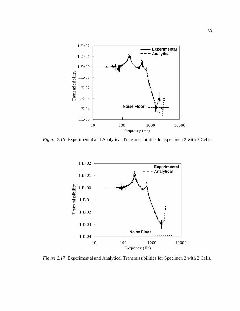
53
.
Figure 2.16: Experimental and Analytical Transmissibilities for Specimen 2 with 3 Cells.
.
Figure 2.17: Experimental and Analytical Transmissibilities for Specimen 2 with 2 Cells.
1.E-05
1.E-04
1.E-03
1.E-02
1.E-01
1.E+00
1.E+01
1.E+02
10 100 1000 10000Frequency (Hz)
Noise Floor
Tra
nsm
issi
bil i
ty
ExperimentalAnalytical
1.E-04
1.E-03
1.E-02
1.E-01
1.E+00
1.E+01
1.E+02
10 100 1000 10000Frequency (Hz)
Noise Floor
Tra
nsm
issi
bili
ty
ExperimentalAnalytical

54
In Figures 2.15-2.18 experimental and analytical transmissibilities are plotted for
Specimen 2, with varying numbers of cells. For the analytical predictions, the same
value of shear modulus was used as determined for Specimen 1. Similar to Specimen 1,
the results for Specimen 2 show a discrepancy between experimental and analytical
results for stop band depth in the 4 cell case. However, the predictions for the 3, 2, and 1
cell cases are nearly colinear with experimental results over the entire frequency range.
In the transmissibility plots, a noise floor of 1.4 x 10⁻⁴ is shown. The noise floor
is calculated using the following relation:
min
max max
( )
( ) ( )top res
bot bot
a aNF
a a= = ( 2.32 )
.
Figure 2.18: Experimental and Analytical Transmissibilities for Specimen 2 with 1 Cell.
1.E-03
1.E-02
1.E-01
1.E+00
1.E+01
1.E+02
10 100 1000 10000Frequency (Hz)
Tra
nsm
issi
bili
ty
ExperimentalAnalytical

55
where amin and amax are the accelerations of the specimen top and bottom, respectively,
and ares is the accelerometer resolution, quoted at 0.005 g. The maximum experimental
acceleration of the specimen base was measured to be 36 g at 1.5 kHz. The minimum
measured transmissibility for the 3 and 4 cell cases may have been obscured by the
presence of a noise floor.
The results in Figures 2.11-2.18 show that the analytical model can accurately
predict the locations of the beginning stop band frequencies, assuming that the correct
material properties are known. The experimental end frequencies are not well-defined
and, as a result, the accuracy of the end frequency prediction is difficult to assess. The
model accurately predicts stop band depths for both 1 cell cases, as well as the 3 and 2
cell cases for Specimen 2. The minimum measured stop band depth for both the 3 and 4
celled cases is a transmissibility of around 1 x 10⁻⁴, or nearly coincident with the noise
floor. Although the minimum measured transmissibility may have been affected by the
noise floor, this attenuation factor of 10,000 would be sufficient for most vibration
control applications.
In Figures 2.19 and 2.20, experimental transmissibilities are compared for
varying number of layers for both Specimens 1 and 2. Comparing the stop band depths
of both the 1 and 2 cell cases, a full order of magnitude of reduction is gained with an
increase of 1 to 2 cells for both specimens. Similarly, increasing from 2 to 3 cells
reduces the transmissibility by an additional order of magnitude for both specimens. The
effect of increasing the number of cells from 3 to 4, however, is not certain because of the
noise floor location. Although the change in stop band depth cannot be reliably measured

56
when going from 3 to 4 cells, the transmissibility roll-off rate following the beginning of
the stop band is significantly increased. A practical design could therefore limit the
minimum number of cells to three or four to ensure a pronounced stop band attenuation
effect.
The effect of increased elastomer damping was also investigated. An additional
layered specimen (3) was constructed that had the same geometry as Specimen 1. An
elastomer with approximately the same shear modulus as that used in Specimen 1, but
with a significantly higher loss factor, was desired. An elastomer having a modulus
nearly identical to that elastomer 1 at low frequencies was thus selected. Upon tuning the
modulus to align the experimental and analytical results, however, it was found to be
400% higher than the low frequency value. Nevertheless, a transmissibility comparison
between Specimens 1 and 3 is made in Figures 2.21 and 2.22. The loss factor of
Figure 2.19: Comparison of Experimental Transmissibilities for Varying Number ofCells for Specimen 1.
1.E-05
1.E-04
1.E-03
1.E-02
1.E-01
1.E+00
1.E+01
1.E+02
10 100 1000 10000
Frequency (Hz)
1 Cell
2 Cells
3 Cells
4 Cells
Noise Floor
Tra
nsm
issi
bil i
ty

57
elastomer 3 was approximately 0.15. The difference between the higher and lower
damping is most noticeable when comparing the first resonance peaks of Specimens 1
and 3. The first peak of Specimen 1 is about a factor of ten higher than that of Specimen
3. Both specimen transmissibilities, however, reach an approximately equal minimum
value between 1 x 10⁻³ and 1 x 10⁻⁴. Although the minimum measured transmissibilities
may coincide with the noise floor, only measurements within a relatively small frequency
range would have been obscured within the stop bands. Also, the transmissibility roll-off
does not change appreciably with higher damping. Therefore, the basic stop band
attenuation characteristics do not appear to be significantly affected by the addition of
modest damping. Modest elastomer damping, however, could help minimize vibration
transmission at frequencies below the stop band.
.
Figure 2.20: Comparison of Experimental Transmissibilities for Varying Number ofCells for Specimen 2.
1.E-05
1.E-04
1.E-03
1.E-02
1.E-01
1.E+00
1.E+01
1.E+02
10 100 1000 10000Frequency (Hz)
1 Cell
2 Cells
3 Cells
4 Cells
Noise Floor
Tra
nsm
issi
bili
ty
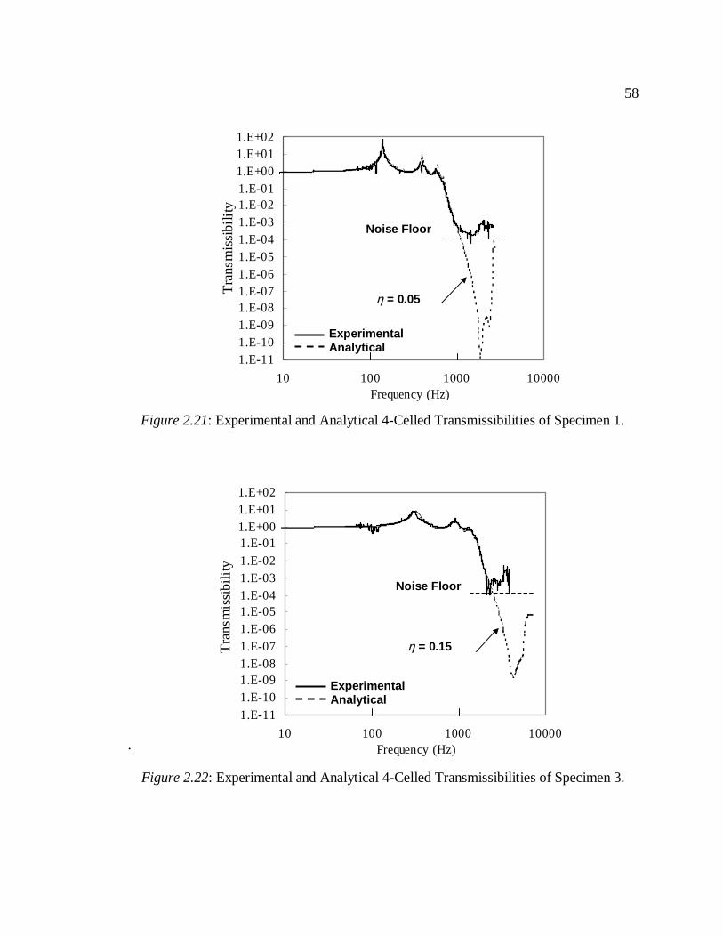
58
Figure 2.21: Experimental and Analytical 4-Celled Transmissibilities of Specimen 1.
.
Figure 2.22: Experimental and Analytical 4-Celled Transmissibilities of Specimen 3.
1.E-111.E-101.E-091.E-081.E-071.E-061.E-051.E-041.E-031.E-021.E-011.E+001.E+011.E+02
10 100 1000 10000Frequency (Hz)
η = 0.05
Noise FloorT
rans
mis
sibi
l ity
ExperimentalAnalytical
1.E-111.E-101.E-091.E-081.E-071.E-061.E-051.E-041.E-031.E-021.E-011.E+001.E+011.E+02
10 100 1000 10000Frequency (Hz)
η = 0.15
Noise Floor
Tra
nsm
issi
bili
ty
ExperimentalAnalytical
Chapter 3
PASSIVE HIGH FREQUENCY GEARBOX ISOLATION
Layered isolators in compression were experimentally validated to exhibit high
frequency transmissibility stop bands. An analytical investigation was then conducted to
determine the feasibility of using layered isolators as helicopter gearbox isolators. The
gearbox design problem was characterized, and the isolator approximation method was
then used in concert with a design optimization routine to determine passive performance
limits of layered isolators.
3.1 Design Constraints
Initial design considerations for helicopter gearbox isolation were investigated. In
particular, design constraints associated with isolator mass, axial stiffness, and
elastomeric fatigue were estimated.

60
3.1.1 Mass Constraints
Soundproofing materials have long been used in helicopter interiors to reduce
cabin noise. Depending on the helicopter’s use as either military or commercial, a certain
amount of added soundproofing mass is generally allowed.
Owen, et al., report that military standards limit the amount of soundproofing
mass to 40-50 lbs. (18-23 kg) [26]. For a helicopter weighting 12,000 lbs., the added
mass is approximately 0.4% of the gross weight. In contrast, it is reported by Marze et
al., that for the VIP versions of the SA 365N Dauphin with a gross weight of 4,000 lbs.,
soundproofing may comprise 2-3% gross weight [24]. This correlates to 80-120 lbs. (36-
54 kg) of added mass.
In correspondence with Sikorsky Corporation, realistic isolator mass constraints
were determined. For a helicopter with gross weight of 12,000 lbs., 50 lbs. of added
soundproofing mass would be acceptable, with 75 lbs. as a maximum. This correlates to
0.4 – 0.6 % gross weight. To ensure a conservative amount of mass added for isolation
purposes, the isolator mass design constraint was chosen to be less than 0.5 % gross
weight of the helicopter in question.
3.1.2 Axial Stiffness Constraints
Typical modern helicopters require gearbox mountings to be nearly rigid to
minimize the relative deflections of the high speed engine-tranmission shafts [53], and to

61
allow for maintenance-free drive shaft couplings [54]. As helicopter gross weight
increases, so do the transmission mount stiffness requirements. In [54], the Bell Model
427 is reported to have quasi-static mount stiffnesses of 13,000 lb/in at two fuselage
connection points, for a total axial stiffness of 26,000 lb/in (4.6 MN/m). The Model 427
has a gross weight of 6,000 lbs. Welsh and fellow researchers retrofitted a modified S-
76B with a ACSR system [53]. The original transmission mounting stiffness at one of
four connection points is reported to be 80,000 lb/in (14 MN/m). The S-76B has a gross
weight of 12,000 lbs. Both transmission mountings are illustrated in Figure 3.1.
The stiffnesses of the proposed layered isolators should be comparable to existing
gearbox support stiffnesses, because they are being considered as possible replacement
mountings in existing helicopter designs. Four different axial stiffness values were
therefore chosen for a series of design runs in the subsequent design optimization
analysis. They are axial stiffnesses of 1, 5, 10, and 15 MN/m (or 5,700 lb/in, 29,000
lb/in, 57,000 lb/in, and 86,000 lb/in).

62
Figure 3.1: Schematic of Helicopter Transmission Mountings.
GW = 12,000 lbs
Typical Stiffness atFour Feet
kaxial = 14 MN/m
Fluidlastic®
Isolatorskaxial = 1.2 MN/m
Bell Model 427 Pylon Isolation System
S-76B Main Gearbox Supports
GW = 6,000 lbs

63
3.1.3 Elastomeric Bearing Stress Constraints
The design of elastomeric bearings has been investigated in numerous references
as applied to helicopter hub bearings and structural engineering applications, particularly
bridge design [55-64]. Natural rubber bearings have been in documented service
supporting bridges for more than 30 years in the United Kingdom and the United States
with no serious reports of deterioration [64]. A typical bridge bearing designed to
account for axial, shearing, and rotational motions in shown in Figure 17.
In 1987, the National Cooperative Highway Research Program published a report
which was intended to develop better understanding of elastomeric bearing behavior, as
well as formulate more rational design specifications [60]. Experimental tests were
performed to assess bearing compression, rotation, shear, stability, fatigue, and low
temperature behavior.
Figure 3.2: 20 year-old layered elastomeric bearing supporting bridge deck in England[64].

64
For bearings fixed against translation (no rotation or shearing), the researchers
report that a conservative value for the maximum compressive stress to avoid bearing
delamination is
2.00( ) 12.00C eG S MPaσ ≤ ≤ ( 3.1 )
where Ge is elastomer shear modulus, and S is shape factor. Similarly, fatigue tests
suggest a maximum dynamic compressive stress of
1.00( )C eG Sσ ≤ ( 3.2 )
Additionally, the metal layers may experience high tensile loading as result of
high compressive stresses in the bearing. Theoretical predictions of the reinforcement
stress were thus determined for circular bearings. A conservative, minimum thickness of
the metal layer to ensure that maximum steel stress is ½ Fy, the yield strength, is
expressed as
1.5(2 )e Cm
y
tt
F
σ≥ ( 3.3 )
where tm is metal thickness, and te is elastomer thickness.
Gembler, et al., reported that BK 177 helicopter strut loads resulting from
momentary flight loads are quite high, and vary from –10 kN to 30 kN [39]. Loads
experienced by different transmission mountings would depend on gross weight and
mounting configuration of the given helicopter. The BK 117 is a medium sized

65
helicopter and for the purposes of determining passive performance limits, 30 kN is
considered the highest quasi-static loading condition to which the layered isolators would
be subjected. Thus, both the preceding stress and thickness constraints have been
implemented in the subsequent layered isolator design cases.
3.2 Design Optimization
An optimization problem that incorporates various isolator parameters and design
constraints is summarized here. The objective of the optimization is to arrive at a design
which minimizes the deviation of the beginning and end frequencies, fB and fE, from
target frequencies, fTB and fTE, while maintaining certain design criteria, such as limits on
axial stiffness, isolator mass, isolator stress, geometry, and material properties. A
schematic describing the design variables is illustrated in Figure 3.3.
A simulated annealing optimization algorithm was developed to solve this
problem. This particular algorithm was chosen because it could be adapted with relative
ease to accommodate the discrete design variable, n, or number of layered cells. The
algorithm finds a solution by repeatedly perturbing the current design variables.
Improved values of the objective function are always accepted and replace the current
design for the next iteration. A more detailed description of this algorithm can be found
in Ref. 65.

66
The optimization problem for the design of layered isolators can be formally
written as
Minimize
TB B TE E
TB TE
abs absf f f f
f fβα +
� � � �� � � �− −� � � �� � � �
� � � �( 3.4 )
Subject to
min 0A Ak k− + ≤ ( 3.5 )
max 0A Ak k− ≤ ( 3.6 )
min 0L Lk k− + ≤ ( 3.7 )
Figure 3.3: Schematic of Design Variables.
Ge, ρe
Gm, ρm
tm
te
hn = 3
d
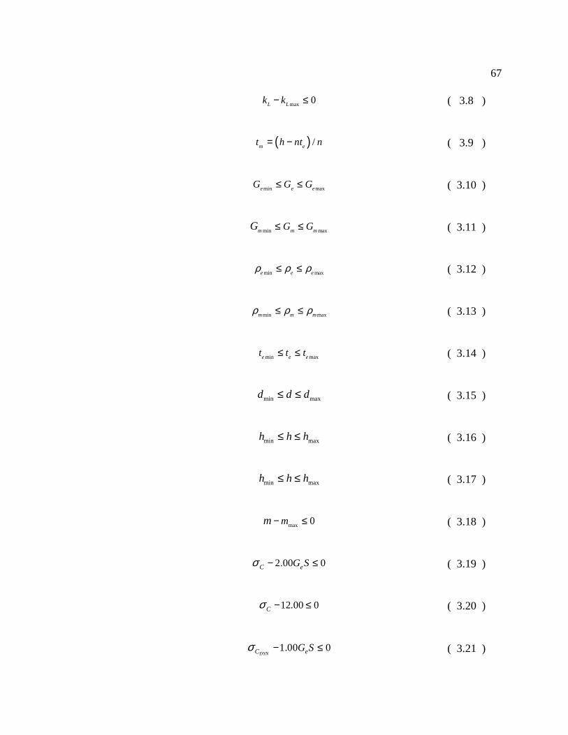
67
max 0L Lk k− ≤ ( 3.8 )
( ) /m et h nt n= − ( 3.9 )
min maxe e eG G G≤ ≤ ( 3.10 )
min maxm m mG GG ≤ ≤ ( 3.11 )
min maxe e eρ ρ ρ≤ ≤ ( 3.12 )
min maxm m mρ ρ ρ≤ ≤ ( 3.13 )
min maxe e et t t≤ ≤ ( 3.14 )
min maxd d d≤ ≤ ( 3.15 )
min maxh h h≤ ≤ ( 3.16 )
min maxh h h≤ ≤ ( 3.17 )
max 0mm − ≤ ( 3.18 )
2.00 0C eG Sσ − ≤ ( 3.19 )
12.00 0Cσ − ≤ ( 3.20 )
1.00 0DYNC eG Sσ − ≤ ( 3.21 )

68
where the design variables are
Ge = Shear modulus of elastomerGm = Shear modulus of metalρe = Density of elastomerρm = Density of metal
te = Thickness of elastomer layerd = Isolator diameterh = Isolator heightn = Number of cells
with constants
fTB = Target beginning frequencyfTE = Target end frequencymmax = Max. isolator massα, β = Weighting factorsGemin,Gemax = Min. and Max. Ge Gmmin, Gmmax = Min. and Max. Gm
ρemin, ρemax = Min. and Max. ρe
ρmmin, ρmmax = Min. and Max. ρm
temin, temax = Min. and Max. te
dmin, demax = Min. and Max. dhmin, hmax = Min. and Max. hnmin, nmax = Min. and Max. nkAmin, kAma x= Min. and Max. axial quasi-static stiffnesskLmin, kLmax = Min. and Max. lateral quasi-static stiffness
and with the intermediate variables
m = Isolator Masstm = Layer thickness of the metalkA = Isolator axial quasi-static stiffnesskL = Isolator lateral quasi-static stiffness
σC = Compressive stressσCDYN = Compressive dynamic stressS = Shape Factor
3.3 Passive Performance Limits
With knowledge of the overall design space for various helicopters, a broad
assessment of the passive performance limits of layered gearbox isolators can be
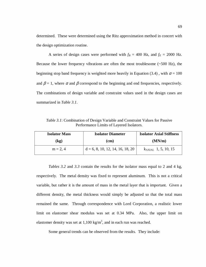
69
determined. These were determined using the Ritz approximation method in concert with
the design optimization routine.
A series of design cases were performed with fB = 400 Hz, and fE = 2000 Hz.
Because the lower frequency vibrations are often the most troublesome (~500 Hz), the
beginning stop band frequency is weighted more heavily in Equation (3.4) , with α = 100
and β = 1, where α and β correspond to the beginning and end frequencies, respectively.
The combinations of design variable and constraint values used in the design cases are
summarized in Table 3.1.
Tables 3.2 and 3.3 contain the results for the isolator mass equal to 2 and 4 kg,
respectively. The metal density was fixed to represent aluminum. This is not a critical
variable, but rather it is the amount of mass in the metal layer that is important. Given a
different density, the metal thickness would simply be adjusted so that the total mass
remained the same. Through correspondence with Lord Corporation, a realistic lower
limit on elastomer shear modulus was set at 0.34 MPa. Also, the upper limit on
elastomer density was set at 1,100 kg/m3, and in each run was reached.
Some general trends can be observed from the results. They include:
Table 3.1: Combination of Design Variable and Constraint Values for PassivePerformance Limits of Layered Isolators.
Isolator Mass
(kg)
Isolator Diameter
(cm)
Isolator Axial Stiffness
(MN/m)
m = 2, 4 d = 6, 8, 10, 12, 14, 16, 18, 20 kAXIAL 1, 5, 10, 15

70
1) For a given mass and stiffness, as diameter increases, the beginning stop band
frequency, fB, is lowered more readily. As diameter is increased, the minimum
axial stiffness constraint can be satisfied with a lower elastomer modulus because
of elastomer shape factor effect. A lower stop band beginning frequency can
therefore be realized more readily at larger diameters.
2) As fB is lowered in the above trend, however, the end frequency, fE, may also be
lowered below the target of 2000 Hz. This is because as the diameter is
increased, the frequency span of the stop band decreases. Because the beginning
frequency was more heavily weighted in the calculations, the stop band is located
closer the beginning target frequency.
3) For a given mass and diameter, as the stiffness constraint increases, the stop band
frequencies increase. This observation might be expected to be caused by the fact
that as the stiffness constraint increases, the elastomer modulus should increase,
and therefore the natural frequencies of the isolator should also increase.
Contrarily, the elastomer modulus actually tends to decrease with increasing axial
stiffness. The results suggest that for higher stiffness isolators, lower stop band
frequencies are possible with thinner elastomer layers having lower modulus
values. For lower stiffness isolators, lower stop band frequencies are possible
with higher modulus elastomers with a higher elastomer thickness.
An important general conclusion which is suggested by Tables 3.2 and 3.3 is that
there often occur cases where the beginning stop band frequencies are above 500 Hz.

71
This frequency is often cited as the beginning of the irritating frequency range emitting
by helicopter gearboxes, and therefore simple layered isolators may not perform
adequately for all design cases. Consequently, an investigation of possible layered
isolator design enhancements was executed to improve isolator performance in the
frequency range immediately below the beginning stop band frequency.

72
Table 3.2: Passive Performance Design Runs, Isolator Mass = 2 kg.
( ) indicates actual optimized value
Axial Stiffness (MN/m)
Stop Band Begin
Frequency (Hz)
Stop Band End
Frequency (Hz)
GELAS
(MPa)
ρ ELAS
(kg/m3)
ρ METAL
(kg/m3)
t ELAS
(cm)t METAL
(cm)
1 (1.17) 739 2369 16.52 1100 2643 4.847 6.6635 1300 5721 5.32 1100 2643 1.213 8.405
10 1753 7396 4.43 1100 2643 0.868 8.54515 (15.87) 2038 7452 1.94 1100 2643 0.548 8.69
1 (1.16) 691 1790 5.65 1100 2643 3.79 3.4335 1127 3465 1.82 1100 2643 1.197 4.517
10 1445 4113 1.21 1100 2643 0.805 4.66715 1895 5619 3.93 1100 2643 1.061 4.576
1 (1.05) 621 1255 3.1 1100 2643 4.06 1.5135 959 2372 1.15 1100 2643 1.373 2.639
10 1191 2916 0.78 1100 2643 0.934 2.81915 1398 3337 0.83 1100 2643 0.827 2.867
1 (1.1) 549 995 1.7 1100 2643 3.846 0.6245 774 1727 0.64 1100 2643 1.425 1.636
10 937 2098 0.44 1100 2643 0.976 1.81415 1052 2341 0.36 1100 2643 0.792 1.901
1 500 969 0.75 1100 2643 2.703 0.5115 628 1327 0.43 1100 2643 1.519 0.993
10 772 1643 0.35 1100 2643 1.113 1.1715 889 1893 0.35 1100 2643 0.97 1.224
1 (3.43) 470 942 0.37 1100 2643 1.975 0.4335 526 1071 0.35 1100 2643 1.688 0.539
10 731 1493 0.62 1100 2643 1.629 0.57415 795 1647 0.46 1100 2643 1.27 0.725
1 (3.66) 418 814 0.34 1100 2643 2.211 0.055 461 914 0.35 1100 2643 1.985 0.164
10 578 1171 0.35 1100 2643 1.558 0.33915 660 1348 0.35 1100 2643 1.353 0.426
1 (9.87) 506 1008 0.34 1100 2643 1.8 0.055 (9.87) 506 1008 0.34 1100 2643 1.8 0.05
10 508 1013 0.34 1100 2643 1.787 0.0515 587 1182 0.37 1100 2643 1.599 0.136
d = 14 cm
d = 16 cm
d = 18 cm
d = 20 cm
d = 6 cm
d = 8 cm
d = 10 cm
d = 12 cm

73
Table 3.3: Passive Performance Design Runs, Isolator Mass = 4 kg.
( ) indicates actual optimized value
Axial Stiffness (MN/m)
Stop Band Begin
Frequency (Hz)
Stop Band End
Frequency (Hz)
GELAS
(MPa)
ρ ELAS
(kg/m3)
ρ METAL
(kg/m3)
t ELAS
(cm)t METAL
(cm)
1 (1.06) 500 2000 25 1015 2643 7.413 14.4245 941 5646 4.51 1100 2643 1.136 17.365
10 1277 7218 3.31 1100 2643 0.78 17.51815 1565 7972 5.02 1100 2643 0.783 17.516
1 472 1608 6.87 1100 2643 4.603 8.1215 886 3570 2.57 1100 2643 1.363 9.465
10 1222 4822 3.41 1100 2643 1.168 9.53515 1481 5843 4.31 1100 2643 1.097 9.578
1 446 1225 3.25 1100 2643 4.255 4.6525 783 2390 1.15 1100 2643 1.371 5.848
10 1050 3020 1.25 1100 2643 1.102 5.95815 1211 3480 0.98 1100 2643 0.877 6.056
1 420 980 1.74 1100 2643 3.931 2.815 672 1701 0.64 1100 2643 1.424 3.865
10 847 2065 0.47 1100 2643 1.002 4.03315 1014 2457 0.59 1100 2643 0.939 4.068
1 (1.16) 400 809 1.26 1100 2643 4.096 1.4995 572 1329 0.44 1100 2643 1.534 2.632
10 738 1677 0.44 1100 2643 1.203 2.75615 1003 2342 1.44 1100 2643 1.582 2.616
1 (1.3) 400 698 1.06 1100 2643 4.363 0.2435 498 1089 0.38 1100 2643 1.74 1.754
10 632 1387 0.37 1100 2643 1.353 1.92915 725 1590 0.36 1100 2643 1.167 2.024
1 (3.31) 400 809 0.43 1100 2643 2.485 0.7235 441 920 0.37 1100 2643 2.023 1.12
10 558 1183 0.37 1100 2643 1.589 1.31115 634 1349 0.34 1100 2643 1.35 1.416
1 (4.75) 400 789 0.39 1100 2643 2.431 0.2495 400 799 0.35 1100 2643 2.291 0.369
10 493 1013 0.35 1100 2643 1.804 0.85215 573 1183 0.39 1100 2643 1.618 0.926
d = 14 cm
d = 16 cm
d = 18 cm
d = 20 cm
d = 6 cm
d = 8 cm
d = 10 cm
d = 12 cm
Chapter 4
DESIGN ENHANCEMENTS FOR IMPROVED ISOLATOR
PERFORMANCE
In the previous chapter, the passive performance of layered isolators was
determined to be inadequate for some design cases. The most apparent performance
limitation was an ability to place the stop band beginning frequency, fB, at low enough
frequencies (~500 Hz), given a set of design constraints. Many active, semi-active, and
passive design enhancements were therefore considered to improve isolator performance
and are briefly summarized here. More specifically, attempts were made to increase the
attenuation at frequencies below fB, and to lower fB to effectively widen the stop band.
4.1 Summary of Active, Semi-Active Concepts to Improve Isolator Performance
The benefits of replacing the conventional elastomer material with
magnetorheological (MR) elastomers were considered. MR elastomers are viscoelastic
solids whose mechanical properties are controllable by applied magnetic fields due to
small iron particles introduced before curing [65-70]. The Young’s modulus has been

75
experimentally observed to increase up to 50% relative to the zero-magnetic-field value.
The change in natural frequency of a given system can be estimated using the familiar
equation /k m . The stop band frequencies could therefore be increased as much as
22% from their zero-magnetic-field values. Because the most critical problem involves
lowering fB, this concept was not pursued.
The performance benefits of replacing the elastomer layers with electrically
shunted layers of either polyvinylidene fluoride (PVDF) or piezoceramic polymer
composites were also investigated. PVDF’s are polymers with modest piezoelectric
coupling effects. Ceramic polymer composites are materials which combine the desirable
properties of piezoelectric sensitivity and mechanical flexibility. This is accomplished by
creating a near-homogeneous solid composed of a piezoceramic and polymer.
Electrically shunting either of these changes their effective stiffness. An expression was
developed for the effective stiffness, k*, of a piezoelectric element undergoing dynamic
strains [71]:
��
�
�
��
�
�
+−+=
)(11
2
2
*
sk
kkk
p
pE
α( 4.1 )
where kE is the effective short circuit material stiffness, kp is the material planar
electromechanical coupling coefficient, α(s) is the nondimensional ratio of the electrical
impedance of the material (i.e. 1/sCpT, where Cp
T is the capacitance of the material
measured under constant stress) to the electrical impedance of the shunt circuit, and s is
the Laplace parameter [72]. Ceramic polymer composites typically have larger

76
electromechanical coupling coefficients than PVDFs, and can range from 0.6 - 0.7.
Using Equation 4.1, this would enable the material stiffness to increase by up to a factor
of 2. This stiffness increase would translate into a 41% increase in stop band frequencies.
Unfortunately, the lowest Young’s modulus possible for these materials is nearly an order
of magnitude higher than that of the elastomer. Therefore, the short circuit stop band
frequencies would be too high, and could only be tuned to higher frequencies. Although
this may be an attractive semi-active approach for other applications, it does not appear
appropriate for helicopter gearbox isolation.
The effectiveness of replacing the metal layers in layered isolators with active
piezoceramic layers was also investigated. The concept was modeled using a one
dimensional finite element model. An open loop control strategy was implemented to
minimize isolator transmissibility by actuating the piezoceramic layers. The small strains
induced in the piezoceramic layers, however, had no visible effect on transmissibility.
For this concept to be effective, the Young’s modulus of the compliant layers must be at
least two orders magnitude below that of the piezoceramic layers.
4.1.1 Emdedded Terfenol-D Actuators in Layered Isolators
The effectiveness of embedding reaction mass actuators in metal layers was
investigated. Terfenol-D actuators have a particularly high force to volume ratio, and an
accurate model of such actuators can be found in [73]. The actuator model was
incorporated into the layered isolator one-dimensional finite element model, and an open

77
loop control strategy was implemented to evaluate the control authority of embedded
actuators. The control strategy was adopted by Anusonti-Inthra [75] from an approach
previously used by Johnson for reduction of low frequency rotor vibrations [74].
In the following example, a single Terfenol-D actuator embedded in the top metal
layer of a three-layered isolator is modeled. A schematic of the model can be seen in
Figure 4.1. The actuator is modeled as a point force, Fa, and the disturbance force, Fb,
acts at the base of the isolator.
The control algorithm is based on the minimization of a quadratic objective
function, J, defined as:
1 2[ ] [ ]TTa aJ x W x F W F= + ( 4.2 )
Figure 4.1: Model Schematic of Layered Isolator with Embedded Terfenol-D Actuator.
Elastomer Layer
Embedded Terfenol-DReaction Mass Actuator
Metal Layer ofLayeredIsolator
x
Fb
Fa

78
where [W1] and [W2] represent penalty weightings on the displacement of the top metal
layer, x, and the actuator force, Fa, respectively. It is assumed that the displacement, x, is
related to the frequency-domain forces, Fa, by the relation
o ax x TF= + ( 4.3 )
where xo is the baseline displacement without actuator force, Fa, and T is the system
transfer matrix. By substituting Eq. 4.2 into Eq. 4.3, a gradient-based method can be
used to minimize J and determine the optimal forces, Fa. By setting / aJ F∂ ∂ = 0, the
optimal input is found to be:
[ ]a oF T x= ( 4.4 )
11 2 1[ ] ([ ] [ ][ ] [ ]) [ ] [ ]T TT T W T W T W−= − + ( 4.5 )
The system transfer matrix, [T], can be determined by perturbing the system with
individual components of actuator force, Fa. The components, Fac and Fa
s, are assumed
to be cosine and sine pairs in the frequency domain, where the superscripts ‘c’ and ‘s’
refer to cosine and sine, respectively. The first column of [T], which corresponds to the
actuator force component Fac, is determined by setting Fa
c to a nonzero value, and the
column is found to be:

79
11
12
cco
ca
sso
ca
x x
Ftt x x
F
� �−� �
� � � �=� � � �−� �� �� �� �
( 4.6 )
Similarly, when Fas has a nonzero value, the second column of [T] is found to be
21
22
cco
sa
sso
sa
x x
Ftt x x
F
� �−� �
� � � �=� � � �−� �� �� �� �
( 4.7 )
Once the cosine and sine components of the actuator force are determined, their
magnitudes are compared to the maximum attainable force predicted by the Terfenol-D
actuator model at that particular frequency to ensure realistic actuator performance. If
necessary, the force components are scaled down to reflect realizable forces.
In Figure 4.2, the transmissibility of a layered isolator is plotted for varying
values of base force, Fb, as well as the case when there is no actuation in the actuator. In
Figure 4.3, the same layered isolator is plotted with and without the embedded actuator
for a base force of 40 N. The relevant isolator properties are te = 1.1 cm, tm = 6.0 cm, Ge
= 1.25 MPa, ρe = 1,100 kg/m3, and the metal layers are aluminum.
In Figure 4.2, the actuator natural frequency is observed to be around 700 Hz and
as expected, the actuator is most effective around this frequency. Points 1 and 3
correspond to the two side resonance peaks associated with a tuned absorber, or the
actuator in this case. Point 2 is the antiresonance frequency caused when no power is
supplied to the actuator, and point 4 corresponds to the beginning of the passive stop

80
band. With increasing base force, the effective actuator bandwidth becomes narrower
around the resonance. The results indicate, however, that an embedded Terfenol-D
reaction mass actuator indeed has the authority to actively cancel vibrations before the
onset of the passive stop band.
Although this control strategy appeared effective, this approach would necessarily
include many of the complexities involved with active control. The search for a purely
passive vibration control solution was therefore continued.
Figure 4.2: Transmissibility of Three-Layered Isolator with Embedded Terfenol-DActuator.
102
103
104
10-8
10-6
10-4
10-2
100
102
Frequency (Hz)
Tra
nsm
issi
bili
ty
Layered
PassiveStop Band
Fb = 20 NFb = 40 NFb = 60 NFb = 80 N
NoActuation
1
2
34

81
4.2 Embedded Vibration Absorbers to Improve Isolator Performance
A passive solution which appeared effective was embedded vibration absorbers,
as illustrated in Figure 4.4. By embedding vibration absorbers in each metal layer of the
isolator, the vibrations occurring at frequencies below the stop band could be attenuated.
As an example, suppose there was a need for an isolator with a diameter of 6 cm, an axial
stiffness of 2.4 MN/m (2 times the stiffness at one gearbox connection on the Bell Model
Figure 4.3: Transmissibility of Isolator with and without Embedded Terfenol-D Actuator.
102
103
104
10-8
10-6
10-4
10-2
100
102
Frequency (Hz)
Tra
nsm
issi
bili
tyPassive
Stop Band
Fb = 40 N, withActuator
NoActuator

82
427), and with a mass less than or equal to 3 kg. The properties of the optimized isolator
are summarized in Table 4.1.
As can be observed in Table 4.1, the stop band beginning frequency, fB, is 684 Hz,
which is too high for the gearbox application. If three embedded absorbers are added to
the isolator, each having a absorber mass of 1 kg, then the isolator will sufficiently
Figure 4.4: Schematic of Layered Isolator with Embedded Vibration Absorbers.
Table 4.1: Optimized Properties of Layered Isolator of Example.
Elastomer LayerStiffness
Embedded VibrationAbsorber
Metal Layer ofLayeredIsolator
VibrationInput
Axial Stiffness (MN/m)
Stop Band Begin
Frequency (Hz)
Stop Band End
Frequency (Hz)
GELAS
(MPa)
ρ ELAS
(kg/m3)
ρ METAL
(kg/m3)
t ELAS
(cm)t METAL
(cm)
2.4 684 2916 0.36 1100 2643 0.587 13.12

83
attenuate over the frequency range of interest. This is illustrated in Figure 4.5. However,
the isolator mass has now been doubled to a value of 6 kg. In general, if conventional
vibration absorbers are used to attenuate frequencies below the stop band, the weight
penalty is prohibitive. Therefore, different means of effectively amplifying the absorber
mass were investigated.
Figure 4.5: Transmissibility of Example Layered Isolator.
101
102
103
104
10-10
10-8
10-6
10-4
10-2
100
102
104
Frequency (Hz)
AbsorberFrequencies
Minimum DesiredAttenuation Level
( < 0.01 )
Without AbsorbersWith Absorbers
Minimum DesiredAttenuation Level
(<0.01)
AbsorberFrequencies

Chapter 5
PERIODICALLY LAYERED ISOLATORS WITH EMBEDDED
INERTIAL AMPLIFIERS
In the previous chapter, a series of design enhancements were considered to
improve isolator performance. The use of embedded vibration absorbers appeared
effective, although they necessitated too much added isolator mass. Several
configurations were therefore considered to effectively amplify absorber mass. An
attractive configuration is illustrated in Figure 5.1. This configuration was found to
exhibit a combination of advantageous benefits, including inertial amplification and
vibration absorber effects. A detailed investigation into the performance effects of these
amplifiers was conducted. The use of embedded fluid elements was determined to be an
efficient method to realize inertial amplification in the isolators.
5.1 Embedded Inertial Amplifiers
The inertial amplification effect can be observed when relative motion occurs
between layers. As the schematic in Figure 5.1 suggests, relative motion necessarily

85
causes the lever arm to rotate, thus causing motion of the tuned mass. Because the tuned
mass is attached to the end of the lever arm, the inertia of the metals layer is effectively
increased when relative motion occurs.
The vibration absorber effect results from interaction between the elastomer layer
stiffness and the tuned mass. At certain tuned frequencies, the isolator will experience
antiresonance conditions independent of layer masses. These tuned frequencies are only
dependent on the amount of tuned mass, length of lever arms, and stiffness of the
elastomer layers.
Consider an inertial amplification element alone, as in Figure 5.2. Equations of
motion can be written for the mechanical system in Figure 5.2, and can be expressed as
2
1
0 0 0 00 0 0 00 0 0t t
uu
m u
� � � � � �� � � �� � =� � � �
� � � � � � � � � �
��
��
��
( 5.1 )
Assuming that R=b/a, a kinematic constraint equation exists that uses the length ratio, R,
to relate the motion of the tuning mass, ut, to the u2, and u1, [54]
1 2( ) ( 1)tu R u R u= − − ( 5.2 )
This constraint equation can be used to reduce the three degree of freedom system to two
degree of freedom system, by first creating a transformation matrix, G, as in
{ } [ ]{ }3 2DOF DOFu G u= ( 5.3 )

86
{ }22
11
1 00 1
1t
uu
uu
u R R
� � � �� � � �=� �
� �� � − � �
( 5.4 )
If the equations of motion in Equation 5.1 are pre and post-multiplied by [G], then the
reduced degree of freedom equations can be written as [54]
{ } { }22
21
( 1) ( 1) 00( 1)
t t
t t
R m R R m uuR R m R m
� �− − − =� �− −� �
��
��
( 5.5 )
In this inertial matrix, the tuned mass is effectively being amplified approximately
by the square of the lever arm ratio, R. An inertial amplifier can be attached to each
metal layer in the three dimensional model by providing appropriate constraint equations
for Equation 5.5.
Figure 5.1: Schematic of Isolator Configuration with Embedded Inertial Amplifiers.
Elastomer LayerStiffness
Embedded Inertial Amplifier
Rigid Link
Metal Layerof Layered
Isolator
Vibration Input
Tuned Mass on LeverArm
ba

87
5.2 Effect of Embedded Inertial Amplifiers on Layered Isolator Frequency Response
The first advantageous effect of these inserted elements is that the relative motion
between layers necessitates relative motion between the lever arm mass and the layers.
This serves to amplify the effective dynamic inertia of the metal layers when relative
motion occurs. This can readily be observed most by examining the first n eigenvalues of
an n-celled isolator with and without embedded inertial amplifiers. In Table 5.1, the first
three eigenvalues of the previous example isolator are listed with and without embedded
inertial amplifiers. The length of the lever arm portions, a and b, and tuned masses are
listed in Table 5.2.
Figure 5.2: Schematic of one inertial amplifier.
a
b
u1
u2
mt R = b / a

88
The beginning stop band frequency, fB, has been lowered to 473 Hz from 684 Hz
with the addition of inertial amplifiers. Because the end stop band mode shape involves
little relative motion between layers, the end frequency is not significantly affected. This
is evidenced by the stop band mode shapes pictured Figure 5.3. The stop band frequency
range has been expanded to include the target frequency range (500 - 2000 Hz). The
differences in tuned mass values can be explained by considering the tuned masses as
part of vibration absorbers. This concept will be explained in the next section.
Table 5.1: Summary of Isolator Eigenvalues with and without Embedded InertialAmplifiers.
Without InertialAmplifiers
Frequency (Hz)
With InertialAmplifiers
Frequency (Hz)
Mode 1 183 180Mode 2 494 383Mode 3 684 473
Table 5.2: Summary of Example Inertial Amplifier Properties.
Tuned Mass(g)
a(cm)
b(cm)
Layer 1 8.3 1 9Layer 2 5.6 1 9Layer 3 1.9 1 9

89
5.3 Vibration Absorber Effect
Consider a subsystem of a layered isolator with masses m1 and m2 and elastomer
spring stiffness, k, and, in addition, an embedded inertial amplifier as in Figure 5.4.
Figure 5.3: Mode Shapes at Beginning and End Stop Band Frequencies of LayeredIsolator with Embedded Inertial Amplifiers.
fb = 473 Hz
m = 8.3 g
m = 5.6 g
m = 1.9 g
fe = 2788 HzStop Band
Little RelativeMotion of MetalLayers at End of
Stop Band
Significant RelativeMotion of Metal
Layers at Beginningof Stop Band

90
The equations of motion for the system shown in Figure 5.4 can written as
{ } { } { }22 2 2
21 11
( 1) ( 1) 00( 1)
t t
t t
m R m R R m u uk ku uk kR R m m R m
� �+ − − − −� �+ =� � � �−− − + � �� �
��
��
( 5.6 )
In order to determine the isolation frequency for which m1 is completely isolated
from the motion of m2 and mt, the motion of m1 is set equal to zero, u1 = 0. Then the
lower homogeneous equation of the reduced set of equations of motion is solved to yield
1
2 ( 1)( )it
kf
R R mπ=
−( 5.7 )
Thus, the frequency for which m1 is isolated is independent of both masses m1 and
m2 [54]. This illustrates how the elastomer layer stiffness and the amplified tuned mass
combine to act as a vibration absorber.
In Figure 5.5, the transmissibility of the example isolator is shown with and
without the embedded inertial amplifiers from Table 5.2. The addition of the inertial
Figure 5.4: Schematic of Subsystem of Layered Isolator with Embedded InertialAmplifier [54].
a
b
u1
u2
mt R = b / a
m2
m1
k

91
amplifiers lowers the first three isolator eigenvalues, and thus increases the size of the
stop band. Three tuned absorber frequencies can also be identified at 509, 612, and 928
Hz.
When traditional, single-degree-of-freedom vibration absorbers are added to
vibrating mechanical systems to attenuate a response at a particular frequency, there are
typically two additional resonance peaks created in the frequency response curve. This
effect can be observed in Figure 4.5, where traditional absorbers were embedded in the
metal layers of the example isolator. This detrimental effect is sometimes mitigated with
the addition of absorber damping.
The configuration proposed in Figure 5.1, however, does not increase the number
of degrees of freedom of the isolator. No additional resonance peaks are created on either
side of the absorber frequencies as a result, and no internal damping is needed to control
the isolator response within the stop band.

92
5.4 Typical Frequency Response Shapes of Isolator with Embedded Amplifiers
In Figure 5.6, the axisymmetric response shapes of the example isolator are
shown for the identified tuned frequencies in Figure 5.5. The first response shape at 509
Hz shows the top embedded inertial amplifier and the top elastomer layer as the active
tuned absorber. As noted in the figure, the vibration absorber effect can be visualized as
the compressed elastomer force nearly canceling the inertial amplifier force on the second
Figure 5.5: Transmissibility of Example Isolator with and without Inertial Amplifiers.
101
102
103
104
10-10
10-8
10-6
10-4
10-2
100
102
Minimum DesiredAttenuation LevelAchieved in TargetFrequency Range
( < 0.01)
Tuned AbsorberFrequencies
1 23
Without InertialAmplifiers
With InertialAmplifiers
Frequency (Hz)
FrequencyRange ofInterest
Without InertialAmplifiers
With InertialAmplifiers
Minimum DesiredAttenuation Level
Achieved in TargetFrequency Range
(<0.01)
Tuned AbsorberFrequencies
FrequencyRange ofInterest
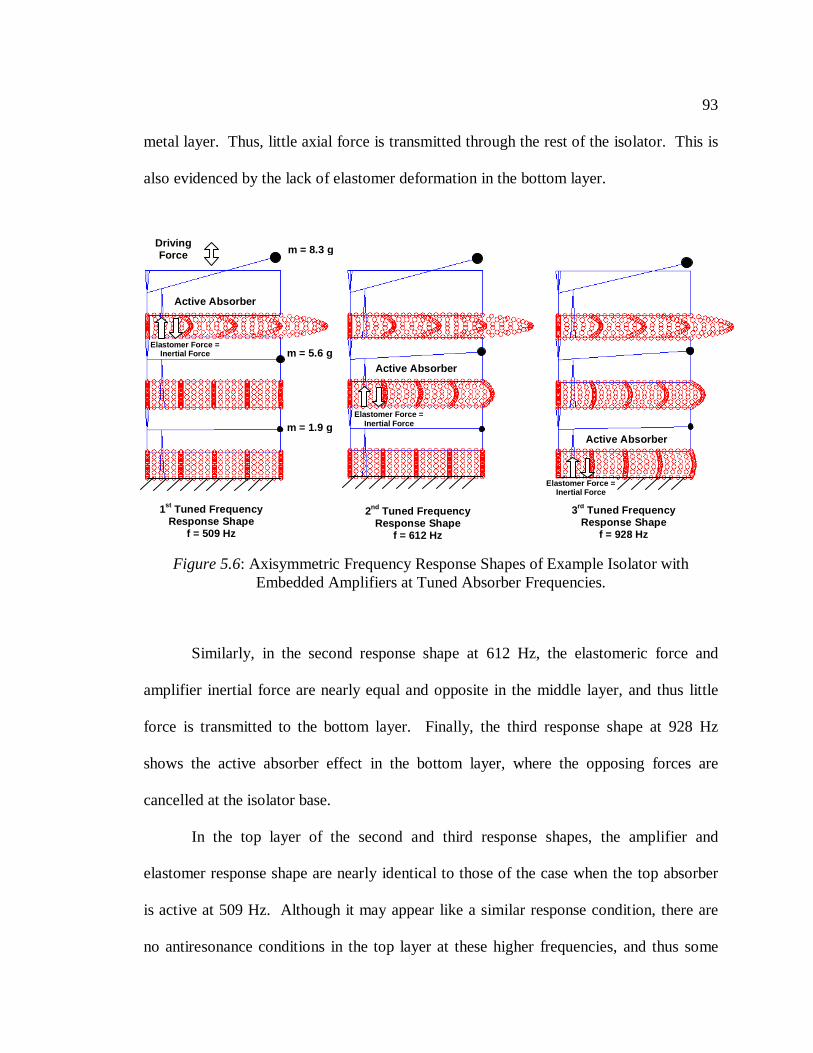
93
metal layer. Thus, little axial force is transmitted through the rest of the isolator. This is
also evidenced by the lack of elastomer deformation in the bottom layer.
Similarly, in the second response shape at 612 Hz, the elastomeric force and
amplifier inertial force are nearly equal and opposite in the middle layer, and thus little
force is transmitted to the bottom layer. Finally, the third response shape at 928 Hz
shows the active absorber effect in the bottom layer, where the opposing forces are
cancelled at the isolator base.
In the top layer of the second and third response shapes, the amplifier and
elastomer response shape are nearly identical to those of the case when the top absorber
is active at 509 Hz. Although it may appear like a similar response condition, there are
no antiresonance conditions in the top layer at these higher frequencies, and thus some
Figure 5.6: Axisymmetric Frequency Response Shapes of Example Isolator withEmbedded Amplifiers at Tuned Absorber Frequencies.
1st Tuned FrequencyResponse Shape
f = 509 Hz
2nd Tuned FrequencyResponse Shape
f = 612 Hz
3rd Tuned FrequencyResponse Shape
f = 928 Hz
DrivingForce
Active Absorber
Active Absorber
Active Absorber
m = 8.3 g
m = 5.6 g
m = 1.9 g
Elastomer Force =Inertial Force
Elastomer Force =Inertial Force
Elastomer Force =Inertial Force
94
force is transmitted to the middle layer. The same comment can be applied to the middle
layer response when the third and second response shapes are compared.
5.5 Effect of Shape Factor and Passive Stop Band Location on Response Behavior
Because of the high axial stiffness design constraint for gearbox isolation,
optimized layered isolator designs often require a relatively high elastomer shape factor
(> 1) for a single layer. For example, a single elastomer layer of the example isolator has
a shape factor of 2.6. Subsequently, the implications of employing a higher elastomer
shape factor for the embedded isolator design will be examined.
5.5.1 High Shape Factor Behavior
In Figure 5.7, response shapes of the example isolator without inertial amplifiers
are shown. Three different frequency locations were chosen to represent typical response
shapes at certain frequencies of interest. The first response shape represents the
frequency range starting at the beginning stop band frequency and ending at the isolator
antiresonance frequency, or point number two. In this region, the dominant mode in the
isolator response is the beginning stop band mode, illustrated in Figure 2.2. This mode
shape is characterized by either uniform axial tension or compression in the elastomer
layer.

95
The second point corresponds to the response shape where the isolator
experiences an antiresonance. The elastomer layers at this frequency exhibit shapes
where the imposed axial motion of the metal layers is translated into radial deformations
and overall isolator dynamic stiffness is at a minimum. This point also corresponds to a
transition in modal dominance, or the point at which the end stop band mode becomes
more dominant. This mode shape is also illustrated in Figure 2.2, and consists of
elastomer deformations that consist of both axial tension and compression within a single
layer.
The third response shape corresponds to this region where the end stop band
mode is most dominant. At higher shape factors, this mode shape is characterized by
little axial motion. Little relative motion between the layers would correspond to little
motion of an embedded amplifier. Consequently, it has been observed through numerous
analytical design cases that embedded inertial amplifiers can only function as vibration
absorbers below this antiresonance frequency, which corresponds to point two in Figure
5.7. It is important to note that this condition only applies to higher shape factor
elastomer layers (� 1). For lower shape factors, different response behavior can be
observed.

96
Figure 5.7: Example Isolator Response Shapes (High Shape Factor, S = 2.6).
Response Shapef = 1142 Hz
Response Shapef = 1652 Hz
Response Shapef = 2745 Hz
101
102
103
104
10-8
10-6
10-4
10-2
100
102
Frequency (Hz)
Tra
nsm
issi
bili
ty
13
2
1 2 3
Frequency Rangefor Possible
AntiresonanceConditions
Minimum ForceTransmitted
DrivingForce

97
5.5.2 Low Shape Factor Behavior
In Figure 5.8, response shapes of the layered isolator described in the first line of
Table 3.3 are illustrated. The elastomer layers in this isolator have a shape factor of 0.2,
which is quite low in comparison to those of other optimized cases. Low shape factors
correspond to thicker elastomer layers, and consequently such isolators exhibit slightly
different dynamics which warrant closer inspection.
Similar to Figure 5.7, the response shapes in Figure 5.8 represent typical response
shapes at certain frequencies of interest. The dominant mode in the first response shape
is the beginning stop band mode. At point two, the response shape corresponds to the
lowest transmissibility exhibited by the isolator. As expected, this response shape
consists of a combination of the beginning and end stop band mode shapes. Contrary to
the higher shape factor isolators, there is no defined antiresonance frequency. Instead,
there is a gradual modal shift toward the end stop band mode shape, as illustrated in the
third response shape. Because of the thicker elastomer layers in this lower shape factor
isolator, there will be more relative axial motion between layers in the vicinity of the end
stop band frequency than in higher shape factor isolators.

98
Figure 5.8: Transmissibility and Response Shapes for Layered Isolator with Shape Factor= 0.2.
101
102
103
104
10-4
10-3
10-2
10-1
100
101
102
103
104
Frequency (Hz)
Tra
nsm
issi
bili
ty
1
3
2
Response Shapef = 820 Hz
Response Shapef = 1425 Hz
Response Shapef = 1902 Hz
1 2 3
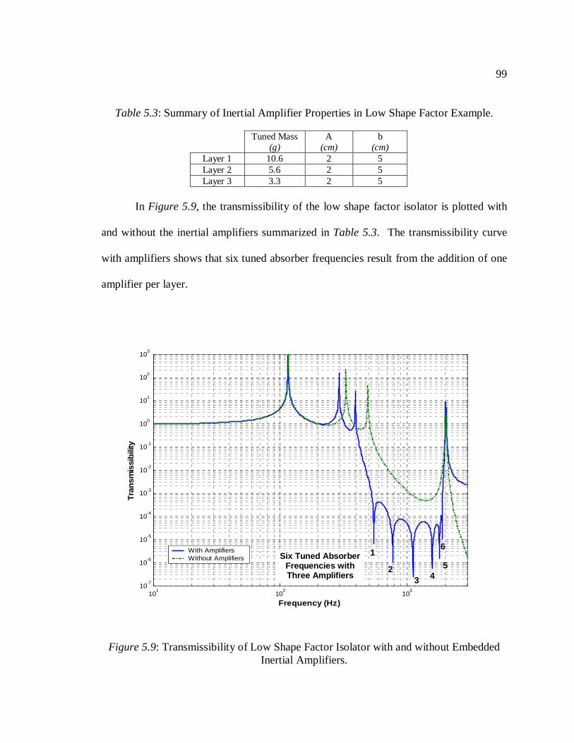
99
In Figure 5.9, the transmissibility of the low shape factor isolator is plotted with
and without the inertial amplifiers summarized in Table 5.3. The transmissibility curve
with amplifiers shows that six tuned absorber frequencies result from the addition of one
amplifier per layer.
Table 5.3: Summary of Inertial Amplifier Properties in Low Shape Factor Example.
Tuned Mass(g)
A(cm)
b(cm)
Layer 1 10.6 2 5Layer 2 5.6 2 5Layer 3 3.3 2 5
Figure 5.9: Transmissibility of Low Shape Factor Isolator with and without EmbeddedInertial Amplifiers.
101
102
103
10-7
10-6
10-5
10-4
10-3
10-2
10-1
100
101
102
103
Frequency (Hz)
Tra
nsm
issi
bili
ty
With AmplifiersWithout Amplifiers
1
23 4
5
6Six Tuned Absorber
Frequencies withThree Amplifiers
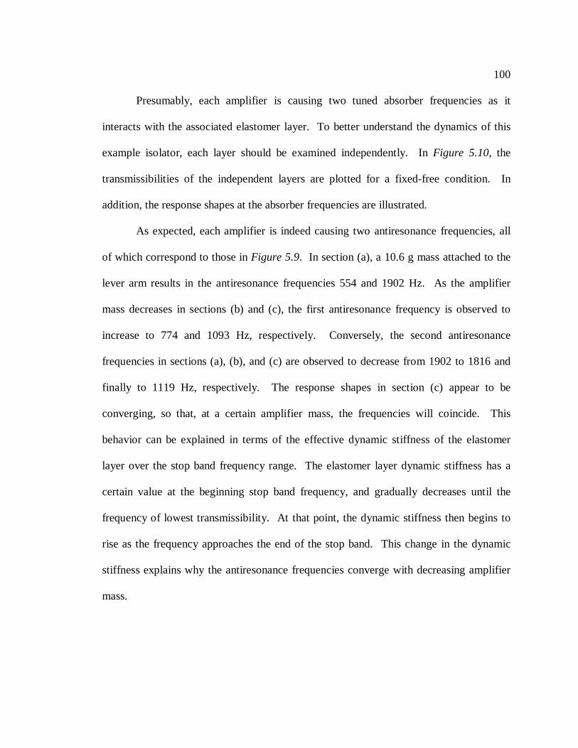
100
Presumably, each amplifier is causing two tuned absorber frequencies as it
interacts with the associated elastomer layer. To better understand the dynamics of this
example isolator, each layer should be examined independently. In Figure 5.10, the
transmissibilities of the independent layers are plotted for a fixed-free condition. In
addition, the response shapes at the absorber frequencies are illustrated.
As expected, each amplifier is indeed causing two antiresonance frequencies, all
of which correspond to those in Figure 5.9. In section (a), a 10.6 g mass attached to the
lever arm results in the antiresonance frequencies 554 and 1902 Hz. As the amplifier
mass decreases in sections (b) and (c), the first antiresonance frequency is observed to
increase to 774 and 1093 Hz, respectively. Conversely, the second antiresonance
frequencies in sections (a), (b), and (c) are observed to decrease from 1902 to 1816 and
finally to 1119 Hz, respectively. The response shapes in section (c) appear to be
converging, so that, at a certain amplifier mass, the frequencies will coincide. This
behavior can be explained in terms of the effective dynamic stiffness of the elastomer
layer over the stop band frequency range. The elastomer layer dynamic stiffness has a
certain value at the beginning stop band frequency, and gradually decreases until the
frequency of lowest transmissibility. At that point, the dynamic stiffness then begins to
rise as the frequency approaches the end of the stop band. This change in the dynamic
stiffness explains why the antiresonance frequencies converge with decreasing amplifier
mass.

101
Figure 5.10: Response Shapes of a Single Layer of the Low Shape Factor ExampleIsolator with Embedded Inertial Amplifiers: (a) m = 10.6 g, (b) m = 5.6 g, (c) m = 3.3 g.
101
102
103
104
10-4
10-3
10-2
10-1
100
101
102
103
Frequency (Hz
Tra
nsm
issi
bili
ty
Response Shapef = 554 Hz
1
Response Shapef = 1902 Hz
2
1 2
101
102
103
104
10-4
10-3
10-2
10-1
100
101
102
103
Frequency (Hz
Tra
nsm
issi
bili
ty
Response Shapef = 774 Hz
1
Response Shapef = 1816 Hz
21
2
101
102
103
104
10-4
10-3
10-2
10-1
100
101
102
103
Frequency (Hz
Tra
nsm
issi
bili
ty
Response Shapef = 1093 Hz
1
Response Shapef = 1119 Hz
21
2
(a)
(b)
(c)
m = 10.6 g
m = 5.6 g
m = 3.3 g
Top Layer
Middle Layer
Bottom Layer

102
5.6 Structural Periodicity of Embedded Amplifier Design
In the previous discussions about the use of embedded inertial amplifiers, the
tuned masses have different values which correspond to different tuned absorber
frequencies. Different values of tuned masses, however, technically result in a loss of
isolator periodicity. It would be useful, therefore, to examine a case where all the tuned
masses are similar.
In Figure 5.11, the transmissibility of the example isolator is plotted with inertial
amplifiers that maintain isolator periodicity, aperiodic inertial amplifiers as described in
Table 5.2, ands the case without inertial amplifiers. The periodic amplifier properties are
listed in Table 5.4. As expected, the periodic amplifiers resonate at the same resonance
frequency, and the attenuation at that frequency is pronounced. Adding aperiodicity to
the amplifiers has the effect of widening the tuned absorber frequency range, but also the
effect of decreasing the attenuation level at the original, center frequency. This behavior
is typical of the effects of adding slight aperiodicities to periodic systems. This figure
also clearly illustrates how the addition of relatively small amounts of periodic amplified
mass in the metal layers results in a dramatic shift in stop band location.
Table 5.4: : Summary of Inertial Amplifier Properties to Maintain Isolator Periodicity.
Tuned Mass(g)
A(cm)
B(cm)
Layer 1 5.6 1 9Layer 2 5.6 1 9Layer 3 5.6 1 9

103
5.7 Passive Stop Band Limitations on Embedded Amplifier Design
Another important observation can be stated regarding Figure 5.9. The isolator
transmissibility curve without embedded amplifiers shows that the passive stop band
frequency range is 500 – 2000 Hz. Although this is the frequency range of interest, the
addition of the amplifiers serves to increase the attenuation of the isolator by nearly two
Figure 5.11: Transmissibility of Example Isolator with and without Inertial Amplifierswhich Maintain Isolator Periodicity.
101
102
103
104
10-8
10-6
10-4
10-2
100
102
Frequency (Hz)
Tra
nsm
issi
bilit
y
Three Co-ResonantAbsorbers
Without InertialAmplifiers
With IdenticalInertial Amplifiers
With Non-identicalInertial Amplifiers

104
orders of magnitude over the entire range. Moreover, numerous analytical case studies
have shown that embedded amplifiers provide maximum attenuation benefits when the
original stop band frequencies span the frequency range of interest.
In Figure 5.5, the layered isolator alone has a stop band ranging from 684 Hz to
2916 Hz. Inertial amplifiers are added to lower the beginning stop band frequency to
below 500 Hz. Although the isolator attenuation is improved at frequencies from 500 to
1000 Hz, the attenuation is diminished from 1000 to 2000 Hz. Absorber performance is
therefore best when the original stop band is as close to the desired range as possible.
The following example will illustrate this point further.
Suppose that the example isolator from Figure 5.5 is now needed to be three
times stiffer, and so an elastomer with a stiffness modulus of three times the initial value
is used. The passive stop band will now range from 1140 Hz to 5011 Hz, as illustrated in
Figure 5.12. Table 5.5 summarizes the amplifier properties which lower the beginning
stop band frequency to 581 Hz.
The length of section b of the lever arm is set to be 6 cm. Because the amount of
amplifier mass should not be prohibitive, the extent to which the beginning stop band can
be lowered is limited. In Figure 5.12, the minimum desired attenuation level is not
achieved over the frequency range of interest. To be most effective, therefore, an isolator
with embedded amplifiers should have an original stop band which spans the desired
frequency range as closely as possible, given physical design constraints.

105
5.8 Fluid Elements as Efficient Implementation of Inertial Amplification
An efficient means of implementing an inertial amplification device, as in Figure
5.4, is in the form of a fluid element. Lord Corporation’s Fluidlastic® mounts, designed
Table 5.5: Summary of Inertial Amplifier Properties in Figure 5.12.
Tuned Mass(g)
a(cm)
b(cm)
Layer 1 19.5 2 6Layer 2 16.7 2 6Layer 3 8.9 2 6
Figure 5.12: Transmissibility of Stiffened Layered Isolator Example with and withoutInertial Amplifiers.
101
102
103
104
10-10
10-8
10-6
10-4
10-2
100
102
Tra
nsm
issi
bili
ty
Frequency (Hz)
With AmplifiersWithout Amplifiers
FrequencyRange ofInterest
MinimumDesired
AttenuationLevel

106
to isolate primary blade passage frequencies, incorporate a dense fluid acting as a tuned
mass of a vibration absorber. A cut-away view of a fluid-filled mount is shown in Figure
5.13 [54].
These fluid-filled mounts consist of an inner cylinder and an outer cylinder
concentrically bonded with elastomers to form two chambers. The chambers are joined
by a tuning port through the inner cylinder which, when filled with a dense, proprietary
fluid, serves as a tuned mass. As the inner cylinder moves up or down, the dense fluid is
forced through the tuning port. The inertial force of the accelerated fluid cancels the
elastomeric spring force at a discrete frequency, or the isolation frequency [54, 76].
Figure 5.13: Cut-Away View of a Fluidlastic® Mount [54].
PARTITIONLESSVOLUME
COMPENSATOR(PAT> PENDING)
UPPER FLUIDRESERVOIR
INNER CYLINDER
ELASTOMERICELEMENTS
TUNINGPORT
LOWER FLUIDRESERVOIR

107
A mechanical analogy, as in Figure 5.4, is helpful in understanding the dynamics
of these mounts. Here, R is the outer-to-inner chamber area ratio, mt is the mass of the
fluid in the tuning port, and k is the elastomeric spring rate in the mount.
In the current work, the main aspect of the fluid-filled mount of interest is the
inertial amplification effect. The elastomeric spring rate would be provided by the
elastomer layer already existing in layered isolators. Therefore, the fluid element would
serve as an inertial amplifier of the metal layers and also serve as part of a vibration
absorber. The isolation frequency would be determined by the stiffness of the elastomer
layer and the amount of mass in the inner chamber of the fluid element.
The diameter of the inner chamber could perhaps be semi-actively altered to
change the tuning frequency. Because transmission noise is tonal in nature, this would be
ideal to improve gearbox isolation performance. Another issue to consider is that fact
that elastomer material properties will change with changing operating conditions.
Causes for material property variation include temperature, frequency, and dynamic
strain. A brief discussion of this issue is provided in Appendix F. As the elastomer
material properties change, the inner cylinder could be tuned to track particularly
irritating disturbances.
Chapter 6
ANALYSIS OF LAYERED ISOLATOR EFFECTIVENESS FOR
GEARBOX ISOLATION
A number of performance benefits were suggested by transmissibility curves of
layered isolators with embedded fluid elements. These plots, however, did not include
the dynamic influence of the helicopter gearbox and fuselage. A more appropriate
isolator characteristic , isolator effectiveness, was therefore defined and calculated in the
case when a layered isolator is placed between a helicopter gearbox and fuselage.
6.1 The Vibration Isolation Problem
The general vibration isolation problem is often characterized by a source, an
isolator, and a receiver, as in Figure 6.1. The components are represented here in terms
of mobility, which is defined as
VM
F= ( 6.1 )
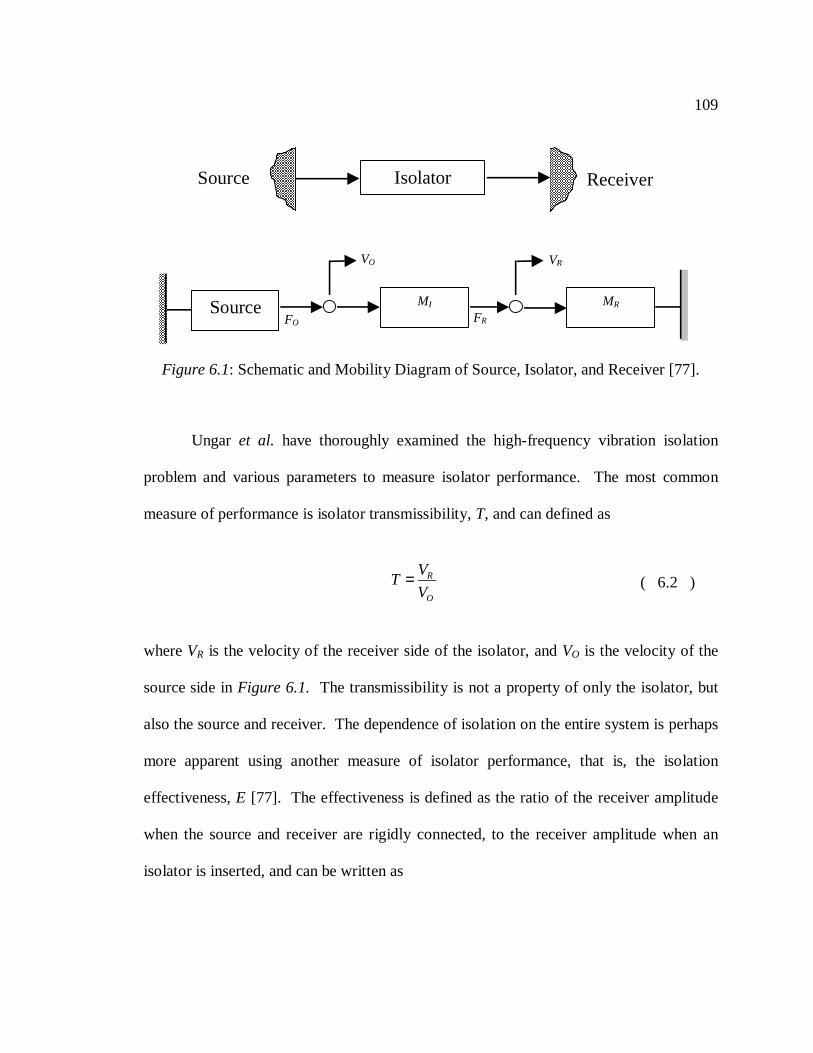
109
Ungar et al. have thoroughly examined the high-frequency vibration isolation
problem and various parameters to measure isolator performance. The most common
measure of performance is isolator transmissibility, T, and can defined as
R
O
VT
V= ( 6.2 )
where VR is the velocity of the receiver side of the isolator, and VO is the velocity of the
source side in Figure 6.1. The transmissibility is not a property of only the isolator, but
also the source and receiver. The dependence of isolation on the entire system is perhaps
more apparent using another measure of isolator performance, that is, the isolation
effectiveness, E [77]. The effectiveness is defined as the ratio of the receiver amplitude
when the source and receiver are rigidly connected, to the receiver amplitude when an
isolator is inserted, and can be written as
Figure 6.1: Schematic and Mobility Diagram of Source, Isolator, and Receiver [77].
IsolatorSource Receiver
MISource MR
VO VR
FO FR

110
RO
R
VE
V= ( 6.3 )
where the subscript O refers to a rigid and massless connection between source and
receiver, and where the absence of the subscript refers to when an isolator is in place.
The effectiveness is thus a measure of how well an isolator performs in a given situation,
with E > 1 corresponding to improved performance as compared to a rigid connection
[77]. If a massless isolator is considered, the isolator effectiveness can be expressed as
1 I
S R
ME
M M= +
+( 6.4 )
Thus, according to Equation 6.4, the isolator mobility, MI, must exceed the sum MS + MR
considerably if the isolator is to be effective.
6.2 Effectiveness of Layered Isolators with Embedded Fluid Elements
6.2.1 Isolator Effectiveness with Non-Negligible Isolator Mass
At high frequencies, the distribution of mass in layered isolators is critical in
defining stop band locations. An expression must be derived which accounts for isolator
mass to accurately predict layered isolator effectiveness, because Equation 6.4 does not
account for mass effects.
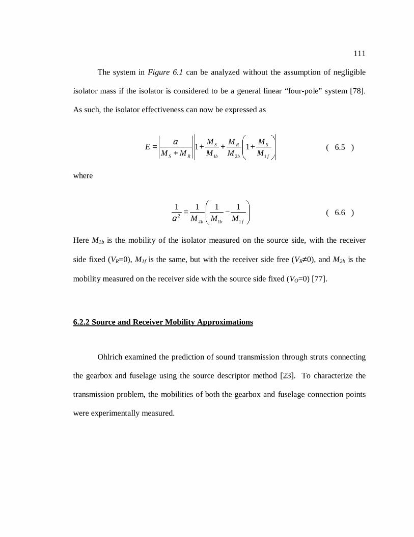
111
The system in Figure 6.1 can be analyzed without the assumption of negligible
isolator mass if the isolator is considered to be a general linear “four-pole” system [78].
As such, the isolator effectiveness can now be expressed as
1 2 1
1 1S SR
S R b b f
M MME
M M M M M
α � �= + + +� �� �+ � �
( 6.5 )
where
22 1 1
1 1 1 1
b b fM M Mα� �
= −� �� �� �
( 6.6 )
Here M1b is the mobility of the isolator measured on the source side, with the receiver
side fixed (VR=0), M1f is the same, but with the receiver side free (VR≠0), and M2b is the
mobility measured on the receiver side with the source side fixed (VO=0) [77].
6.2.2 Source and Receiver Mobility Approximations
Ohlrich examined the prediction of sound transmission through struts connecting
the gearbox and fuselage using the source descriptor method [23]. To characterize the
transmission problem, the mobilities of both the gearbox and fuselage connection points
were experimentally measured.

112
In Figure 6.2, the gearbox (source) and strut/fuselage (receiver) experimental
mobilities of a realistic ¾ -scale laboratory model of a medium sized BK117 helicopter
are plotted [23]. The experimental values were approximated linearly in log space.
These approximations were used to assess the potential effectiveness of a layered isolator
with embedded fluid elements placed in between the gearbox and fuselage.
6.2.3 Layered Isolator Effectiveness Prediction
The mobilities M1b, M1f , and M2b of the layered isolator with embedded fluid
elements described in the previous chapter can be calculated using the isolator model, and
are plotted in Figure 6.3.
Figure 6.2: Experimental Source and Receiver Mobilities: (a) … Experimental, z dir., - - -Approximation, z dir. (b) …. Experimental, z dir., - - - Approximation, z dir. [23].
Gearbox
ConnectionPoint Strut
ConnectionPoint
Fuselage
MS MR

113
The effectiveness of the isolator can then be calculated using Equations 6.5 and
6.6, and is plotted in Figure 6.4. For much of the frequency range of interest, namely 500
– 2000 Hz, the effectiveness has a value of at least 200. At tuned isolator frequencies, the
effectiveness can exceed 1000, and approach 10,000. Therefore, layered isolators with
embedded fluid elements could provide a passive or perhaps semi-active noise control
solution over a wide frequency band. Additionally, the fluid ports could be tuned to track
tonal gearbox disturbances and would enable high isolator effectiveness at discrete
frequencies.
Figure 6.3: Mobilities of Layered Isolator with Embedded Fluid Elements.
100
101
102
103
104
105
10-6
10-5
10-4
10-3
10-2
10-1
Mo
bilit
y, (
m/N
s)
Frequency (Hz)
M1bM1fM2b

114
Figure 6.4: Analytical Effectiveness of Layered Isolator with Embedded Fluid Elements.
102
103
104
100
101
102
103
104
Frequency (Hz)
Effe
ctiv
enes
s
TargetFrequency
Range

Chapter 7
EXPERIMENTAL VALIDATION OF FLUID-FILLED ISOLATOR
CONCEPT
Analytical predictions suggested that fluid elements could be employed as high
frequency inertial amplifiers. Experimental specimens were therefore designed,
fabricated, and tested to validate the analytical results. The experimental
transmissibilities of a set of fluidic layered specimens were obtained and compared to
their predicted transmissibilities.
7.1 Single-Celled Fluidic Specimen Testing
Before building a multi-layered isolator with embedded fluid elements, a single-
celled specimen was first designed and constructed to experimentally validate the
concept. In Figure 7.2 , a schematic and cross-sectional view of such a single-celled
specimen is shown. The specimen was constructed using aluminum and elastomer parts,
and water was used as the tuning fluid.

116
To produce accurate analytical predictions of the specimen’s behavior, the
elastomer material properties needed to be experimentally estimated. This was
accomplished using a simpler one-celled specimen with the same elastomer material,
illustrated in Figure 7.1. The elastomer density was measured to be 1,029 kg/m3, and the
Poisson’s ratio was assumed to be 0.499, or that of a nearly incompressible solid. The
analytical transmissibility curve, generated using the axisymmetric model, was then
positioned to match the experimental results by adjusting the shear modulus and
hysteretic loss factor. The shear modulus and loss factor which provided a reasonable fit
were 1.05 MPa and 0.12, respectively.
Figure 7.1: Transmissibility and Schematic of Single-Celled Specimen to CharacterizeElastomer.
1.E-03
1.E-02
1.E-01
1.E+00
1.E+01
100 1000 10000Frequency (Hz)
Tra
nsm
issi
bili
ty
Experimental
Analytical
To Shaker
Steel Layer
ElastomerLayer
Accelerometers1“

117
The experimental results for both specimens were obtained by attaching the
specimen to a rigid base, which in turn was attached to a mechanical shaker. The shaker
input was a series of chirp signals each spanning 200 Hz. To measure the transmissibility
of a test specimen, one accelerometer was placed on top of the metal layer, and another
was placed on the rigid base. The signals were then fed into a Fourier analyzer. In this
way, the specimen transmissibilities were directly measured.
Figure 7.2: Single-Layered Specimen with Embedded Fluid Element: (a) Illustration, (b)Cross-section.
InnerCylinder
OuterCylinder
VolumeCompensa
torFlexibleSeals
ElastomerLayer
RigidLinks
TuningPort
PressureValve
To Shaker
(a) (b)
11/4“
3/8“
1 3/4“
1 1/4“

118
Both the experimental and analytical transmissibilities for the specimen pictured
in Figure 7.2 are plotted in Figure 7.3. The curves are nearly coincident for frequencies
greater than 400 Hz, and both indicate a tuned resonance condition near 600 Hz. Two
distinct resonance peaks, however, can be observed in the experimental plot, whereas
only one is predicted analytically. This discrepancy may be due to the fact that the all
parts of the specimen are considered rigid in the model. In reality, the rigid links and
inner cylinder may not be stiff enough at high frequencies to be considered rigid, and
therefore their dynamics may not be captured in the model.
Figure 7.3: Analytical and Experimental Transmissibilities of Single-Layered Specimenwith Embedded Fluid Element.
1.E-02
1.E-01
1.E+00
1.E+01
10 100 1000Frequency (Hz)
Tra
nsm
issi
bili
ty
Experimental
Analytical
AbsorberFrequency

119
Problems with the flexible seals visible in the cross-sectional view in Figure 7.2
rendered more extensive experimental tests of this specimen difficult. Through
correspondence with Lord Corporation, a suggested internal pressure of 10 – 50 psi was
advised to ensure the desired fluid effect. The seals, however, would fail after being
exposed to a pressure of 10 psi for approximately ten minutes. The results in Figure 7.3,
however, indicate that embedded fluid elements are capable of functioning as mass
amplifying elements at high frequencies.
7.2 Three-Celled Fluidic Specimen Testing
As a result of the previous encouraging test, the design of a three-celled specimen
with fluid elements was initiated, the purpose of which would be to validate the predicted
performance benefits of fluid elements in a multi-layered specimen. Preliminary designs
were completed at Penn State in collaboration with Lord Corporation design engineers.
The final technical drawings for the specimen parts are illustrated in Appendix 5, and
were produced using Ironcad design software.
A cross section of the final design is illustrated in Figure 7.4. The design consists
of three cells, with a fluid element embedded in each metal layer. An individual cell
consists of an inner cylinder, which is rigidly connected to the layer below via two rigid
links on opposite sides. The inner diameter is gradually increased at either side of the
cylinder, to minimize fluid viscous effects. The inner cylinder is connected to the outer

120
cylinder by what is ideally a perfectly flexible seal. As a first attempt to satisfy this
design criterion, the original specimen configuration was designed using reinforced fabric
material. Reinforced fabric was presumed to be quite flexible in the configuration shown
in Figure 7.4, but also to resist any bulging that might be caused by fluid pressure
variations. This behavior is important to ensure that fluid is forced anuularly through the
inner cylinder. The design also includes a fluid reservoir which is separated from the
inner cylinder by a orifice plate, and allows for the fluid to be pressurized. The elastomer
was chosen to be similar to that used in previous specimens to help predict specimen
performance. The original design also specified Lord’s proprietary dense fluid to be
used, which has a density of 1,770 kg/m3. Although all the inner diameters in Figure 7.4
are illustrated as equal, Table 7.1 lists actual dimensions.

121
Figure 7.4: Cross-sectional View of Three-celled Specimen with Embedded FluidElements.
InnerCylinder
OuterCylinder
VolumeCompensator
Flexible Seals (k~0)
ElastomerLayer
RigidLinks
TuningPort
To Shaker
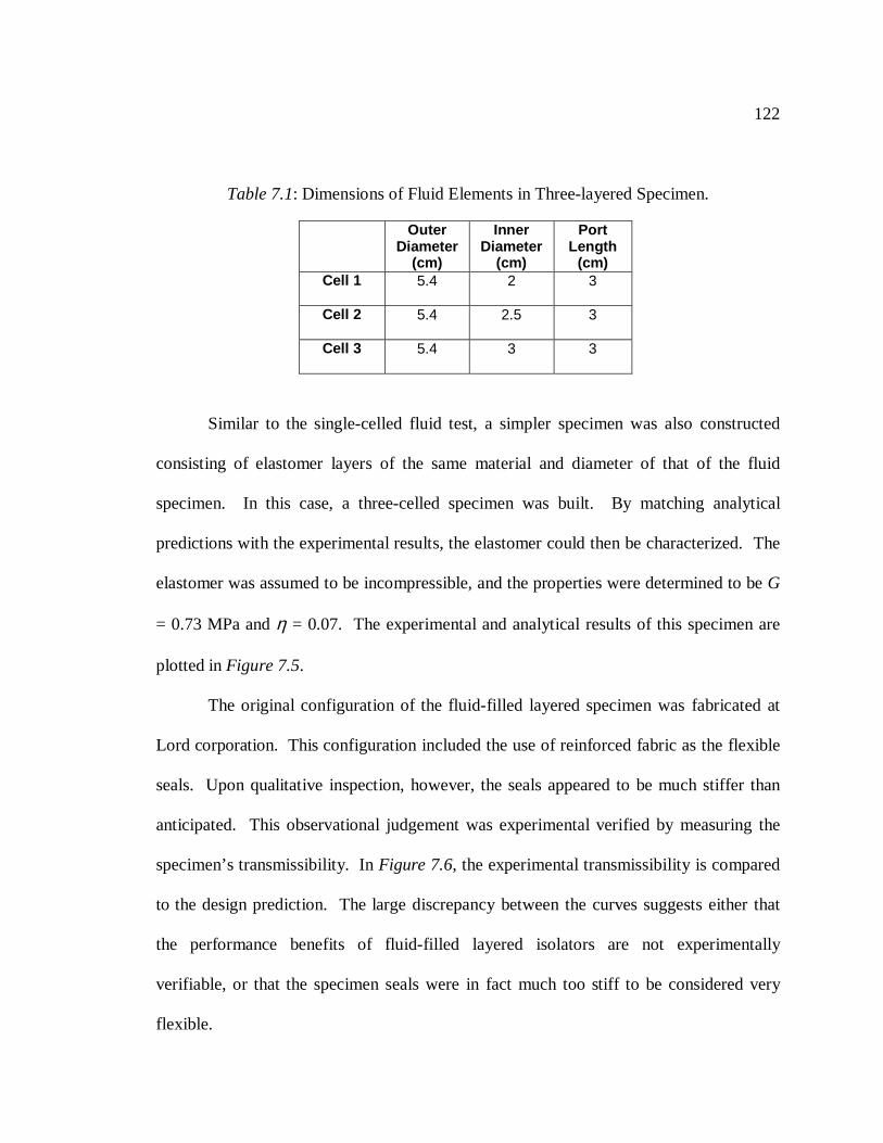
122
Similar to the single-celled fluid test, a simpler specimen was also constructed
consisting of elastomer layers of the same material and diameter of that of the fluid
specimen. In this case, a three-celled specimen was built. By matching analytical
predictions with the experimental results, the elastomer could then be characterized. The
elastomer was assumed to be incompressible, and the properties were determined to be G
= 0.73 MPa and η = 0.07. The experimental and analytical results of this specimen are
plotted in Figure 7.5.
The original configuration of the fluid-filled layered specimen was fabricated at
Lord corporation. This configuration included the use of reinforced fabric as the flexible
seals. Upon qualitative inspection, however, the seals appeared to be much stiffer than
anticipated. This observational judgement was experimental verified by measuring the
specimen’s transmissibility. In Figure 7.6, the experimental transmissibility is compared
to the design prediction. The large discrepancy between the curves suggests either that
the performance benefits of fluid-filled layered isolators are not experimentally
verifiable, or that the specimen seals were in fact much too stiff to be considered very
flexible.
Table 7.1: Dimensions of Fluid Elements in Three-layered Specimen.
OuterDiameter
(cm)
InnerDiameter
(cm)
PortLength
(cm)Cell 1 5.4 2 3
Cell 2 5.4 2.5 3
Cell 3 5.4 3 3
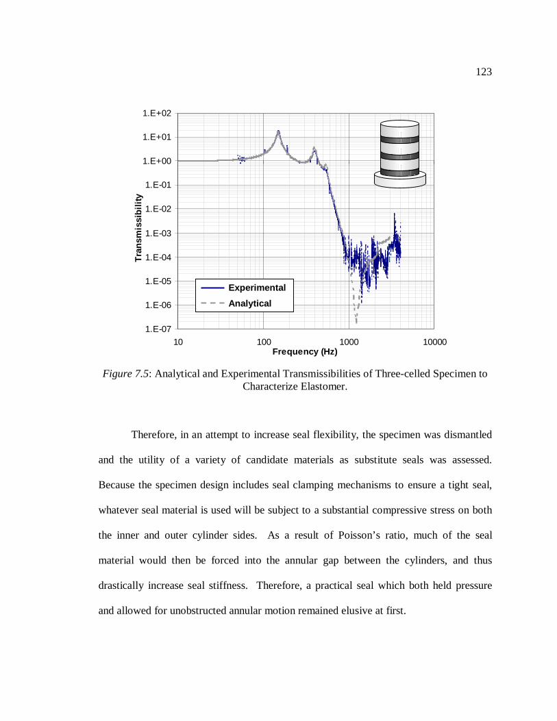
123
Therefore, in an attempt to increase seal flexibility, the specimen was dismantled
and the utility of a variety of candidate materials as substitute seals was assessed.
Because the specimen design includes seal clamping mechanisms to ensure a tight seal,
whatever seal material is used will be subject to a substantial compressive stress on both
the inner and outer cylinder sides. As a result of Poisson’s ratio, much of the seal
material would then be forced into the annular gap between the cylinders, and thus
drastically increase seal stiffness. Therefore, a practical seal which both held pressure
and allowed for unobstructed annular motion remained elusive at first.
Figure 7.5: Analytical and Experimental Transmissibilities of Three-celled Specimen toCharacterize Elastomer.
1.E-07
1.E-06
1.E-05
1.E-04
1.E-03
1.E-02
1.E-01
1.E+00
1.E+01
1.E+02
10 100 1000 10000Frequency (Hz)
Tra
nsm
issi
bil
ity
Experimental
Analytical

124
The first material tried was a very flexible elastomer with the same thickness as
the reinforced fabric. This material choice resulted in the identification of the Poisson’s
ratio bulging effect, and consequently a variety of other materials were tried. The next
material used was a bicycle inner tube rubber with a thickness of 1/32”, or about half of
the original reinforced fabric thickness. The bulging effect, however, remained a
problem with this material, as well. Next, a gasket material used to seal pipe joints with a
1/32” thickness was chosen. Because this material was more stiff than the inner tube
rubber, it was desired to minimize the bulging effect. Unfortunately, this material also
failed to provide the necessary flexibility. It was concluded that a much thinner seal
material would be needed.
Figure 7.6: Experimental and Analytical Transmissibility Comparison of Original Three-celled Configuration.
1.E-05
1.E-04
1.E-03
1.E-02
1.E-01
1.E+00
1.E+01
1.E+02
10 100 1000 10000Frequency (Hz)
Tra
nsm
issi
bil
ity
Experimental
Analytical
PredictedAbsorber
Frequencies
PerformanceDiscrepancy
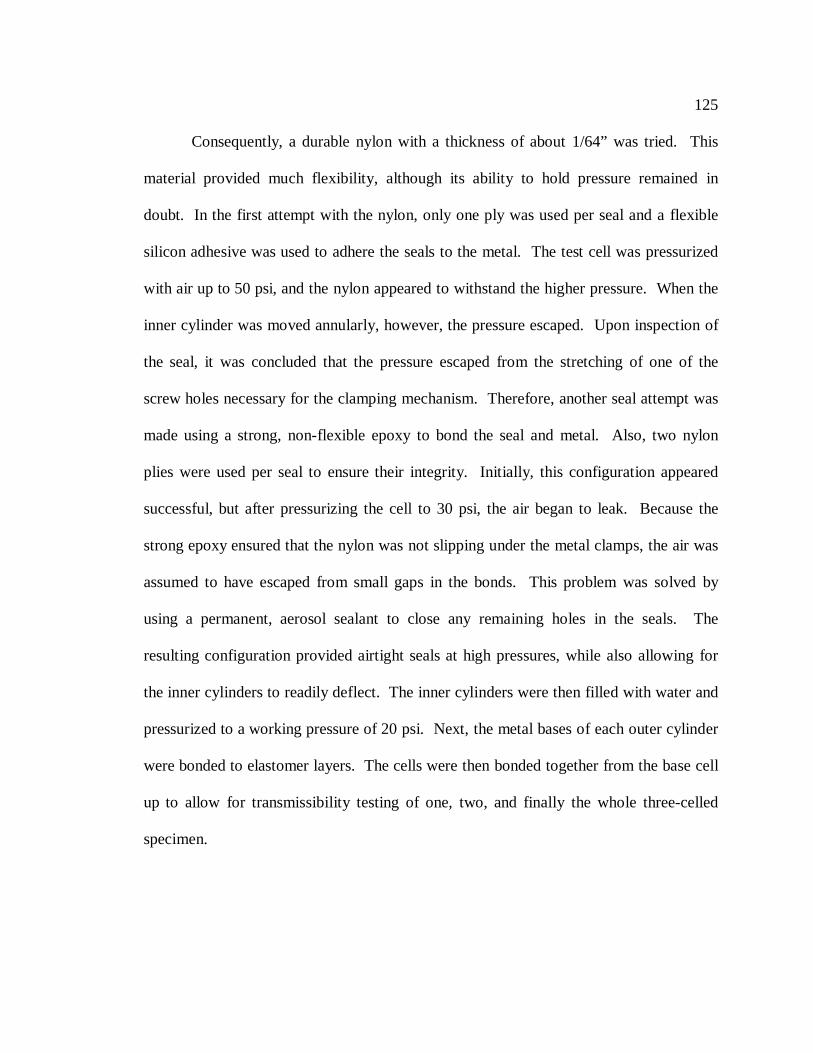
125
Consequently, a durable nylon with a thickness of about 1/64” was tried. This
material provided much flexibility, although its ability to hold pressure remained in
doubt. In the first attempt with the nylon, only one ply was used per seal and a flexible
silicon adhesive was used to adhere the seals to the metal. The test cell was pressurized
with air up to 50 psi, and the nylon appeared to withstand the higher pressure. When the
inner cylinder was moved annularly, however, the pressure escaped. Upon inspection of
the seal, it was concluded that the pressure escaped from the stretching of one of the
screw holes necessary for the clamping mechanism. Therefore, another seal attempt was
made using a strong, non-flexible epoxy to bond the seal and metal. Also, two nylon
plies were used per seal to ensure their integrity. Initially, this configuration appeared
successful, but after pressurizing the cell to 30 psi, the air began to leak. Because the
strong epoxy ensured that the nylon was not slipping under the metal clamps, the air was
assumed to have escaped from small gaps in the bonds. This problem was solved by
using a permanent, aerosol sealant to close any remaining holes in the seals. The
resulting configuration provided airtight seals at high pressures, while also allowing for
the inner cylinders to readily deflect. The inner cylinders were then filled with water and
pressurized to a working pressure of 20 psi. Next, the metal bases of each outer cylinder
were bonded to elastomer layers. The cells were then bonded together from the base cell
up to allow for transmissibility testing of one, two, and finally the whole three-celled
specimen.

126
In Figure 7.7, the analytical and experimental transmissibilities of the base cell
are plotted. The fluid element dimensions in the analytical model are again those listed in
Table 7.1, with the base cell denoted as Cell 3. The fluid density is now that of water, or
1,000 kg/m3. The mass of the outer cylinder and connected inner parts was measured to
be 1.4 kg. As can observed in the figure, both curves agree quite well for frequencies
below the tuned absorber frequency at around 700 Hz. After the absorber frequency,
however, the experimental plot rises at a steeper slope than the analytical. This
discrepancy may be a result of failing to accurately model the fluid dynamics after the
anitresonance point, such as not accounting for wave dynamics of the water.
Figure 7.7: Analytical and Experimental Transmissibilities of Single-celled Specimenwith Embedded Fluid Element.
1.E-02
1.E-01
1.E+00
1.E+01
1.E+02
10 100 1000 10000Frequency (Hz)
Tra
nsm
issi
bil
ity
Experimental
Analytical AbsorberFrequency

127
For instance, the tuning port of the inner cylinder is bound on both sides by flat
surfaces, and the fluid can be considered as a simple column of water bound on both
ends. In a simple column of fluid, standing waves develop at certain resonance
frequencies when excited. Standing waves occurring in the fluidic isolator could cause
an increase in the overall isolator transmissibility.
The lowest frequency in which a standing wave could occur is given by
11 2w wc c
fLλ
= = ( 7.1 )
where f1 is the first standing wave frequency, λ1 is the associated wavelength, cw is the
speed of sound in water at 20° C (1482 m/s), and L is the total length of the inner column
of water. For inner column length of L = 0.043 m, the first standing wave frequency is f1
= 17,300 Hz. The frequency range of interest for these isolators is 500 – 2000 Hz, and
therefore axial standing waves should not be the cause of the transmissibility
discrepancy. Coupling of the lateral and axial motion of the water, however, may be the
cause. A detailed computational analysis of the fluid dynamics may be necessary to
determine how the fluid motion may be affecting the measured isolator transmissibility.

128
In Figure 7.8, the analytical and experimental transmissibilities of two cells (Cells
2 and 3 in Table 7.1) are plotted. Again, good agreement can be observed between the
two curves before the absorber frequencies, which the analytical model predicts to be
around 600 and 700 Hz. At higher frequencies the transmissibilities once more diverge.
The roll-off rate of the two-celled specimen is significantly higher than the one-celled
case, as can be observed in Figure 7.10. It should be noted that the metal layer mass of
the base cell has now increased to 2.0 kg because of the addition of the rigid links and
also the inner cylinder of the second cell, which are both rigidly connected to the base
outer cylinder.
Figure 7.8: Analytical and Experimental Transmissibilities of Two-celled Specimen withEmbedded Fluid Elements.
1.E-04
1.E-03
1.E-02
1.E-01
1.E+00
1.E+01
1.E+02
10 100 1000 10000Frequency (Hz)
Tra
nsm
issi
bil
ity
Experimental
AnalyticalAbsorber
Frequencies

129
Finally, the analytical and experimental transmissibilities of the entire three-celled
specimen are plotted in Figure 7.9. As with the previous two figures, the two curves
indicate a close agreement between predicted and actual performance. Tuned absorber
frequencies are observed in the experimental plot at 500, 600, and 700 Hz, but are not
well defined due to elastomer hysteretic damping. Again, the experimental
transmissibility rises faster than the analytical after the absorber frequencies. A more
detailed model may be required to accurately capture the fluid dynamics at these higher
frequencies. However, the basic predicted performance benefits of embedded fluid
elements in layered isolators are clearly validated. Namely, they are the inertial
amplification effect to lower the first n isolator eigenvalues and the tuned absorber effect.
Figure 7.9: Analytical and Experimental Transmissibilities of Three-celled Specimenwith Embedded Fluid Elements.
1.E-05
1.E-04
1.E-03
1.E-02
1.E-01
1.E+00
1.E+01
1.E+02
10 100 1000 10000Frequency (Hz)
Tra
nsm
issi
bil
ity
Experimental
Analytical
AbsorberFrequencies

130
In Figure 7.10, the experimental transmissibilities of the one, two, and three-
celled fluid-filled specimens are compared. Similar to earlier tests of non-fluidic
specimens with differing number of cells, the addition of cells lowers the attenuation in
the stop band and increases the initial roll-off rate of the stop band. Also, the tuned
absorber frequencies do not change with the addition of more cells, but the attenuation at
those frequencies increases with increasing cells.
The effect of the fluid elements on specimen transmissibility can be observed in
Figure 7.11. If the fluid elements are removed in the analytical model, then the
beginning stop band frequency will be increased from 340 to 460 Hz. Additionally, there
will be no absorber effect at discrete frequencies.
Figure 7.10: Experimental Transmissibility Comparison of One, Two, and Three-celledSpecimens with Embedded Fluid Elements.
1.E-05
1.E-04
1.E-03
1.E-02
1.E-01
1.E+00
1.E+01
1.E+02
10 100 1000 10000
Frequency (Hz)
Tra
nsm
issi
bil
ity
1 Cell
2 Cells
3 Cells

131
In Figure 7.12, the specimen transmissibilities for the original Lord configuration
and the rebuilt configuration are plotted. Because the fluid in the original configuration
is nearly twice as dense as the water used the rebuilt version, the model predicts that the
original version should have a lower frequency stop band than the latter version. In the
figure, however, the original configuration is clearly much stiffer than the second
configuration, indicating that the reinforced fabric seals are not appropriate for this
application. This comparison serves to emphasize the importance of constructing such
isolators with seals that have very low stiffness relative to the elastomer layers.
Figure 7.11: Transmissibility Comparison of Three-celled Specimen with and withoutEmbedded Fluid Elements.
1.E-08
1.E-07
1.E-06
1.E-05
1.E-04
1.E-03
1.E-02
1.E-01
1.E+00
1.E+01
1.E+02
10 100 1000 10000Frequency (Hz)
Tra
nsm
issi
bil
ity
AbsorberFrequencies
Experimental (Fluid)
Analytical (Fluid)
Analytical (No Fluid Elements)

132
Figure 7.12: Transmissibilities of Three-Celled Specimen in Original Configuration andRebuilt Configuration.
1.E-05
1.E-04
1.E-03
1.E-02
1.E-01
1.E+00
1.E+01
1.E+02
10 100 1000 10000Frequency (Hz)
Tra
nsm
issi
bil
ity
Original Configuration
Rebuilt Configuration

133
Chapter 8
CONCLUSIONS AND RECOMMENDATIONS FOR FUTURE WORK
8.1 Conclusions
A Ritz approximation method was developed to model the axisymmetric dynamic
behavior of layered isolators. A single cell was modeled in a fixed-free condition, the
first two modes of which are subsequently used to provide estimates for the beginning
and end stop band frequencies. To accurately predict the first two natural frequencies of
a cell to within 5% error, a certain minimum power of the variables, ‘r’ and ‘z’, was
required for the both the radial and axial directions. For the radial direction, the powers
of ‘r’ and ‘z’ were two and three, respectively. For the axial direction, they were one and
four, respectively.
An n-celled isolator model was developed using the Ritz approximation method
combined with a modal synthesis method. The natural frequencies were found to agree
with 2-D axisymmetric finite element predictions. The model enabled the prediction the

134
nth and (n+1)th isolator modes, which correspond to the stop band beginning and end
frequencies.
The isolator model was validated with experiments. Experimental and analytical
transmissibilities were compared for two specimens with the same elastomer, but
different shape factors. The elastomer properties used for analytical predictions were
determined by matching analytical and experimental transmissibilities of the first
specimen. The properties were then used to predict the behavior of the second specimen.
In both cases, the transmissibilities before the start of the stop band show close
agreement. For the four and three cell cases, analytical transmissibilities lie below the
experimental results, although the experimental noise floor may affect these results. A
minimum experimental transmissibility of about 1 x 10⁻⁴ was observed for these three and
four cell cases.
Experimental and analytical transmissibilities were also compared for two
specimens fabricated with two different low modulus elastomers, one highly damped, and
one lowly damped. The experimental results show that stop band effectiveness is not
appreciably affected by addition of modest damping.
The physical design constraints of the proposed helicopter gearbox isolators were
estimated. Namely, constraints associated with isolator mass, axial stiffness, geometry,
and elastomeric fatigue were gathered from the literature and correspondence with
industry. The passive performance limits of layered isolators were then determined using
a design optimization methodology employing a simulated annealing algorithm. A series
of design runs were performed with target beginning and end stop band frequencies of

135
400 Hz and 2000 Hz, respectively. The results suggest that layered isolators cannot
always meet frequency targets given a certain set of design constraints. Most commonly,
the beginning stop band frequency cannot be lowered sufficiently to attenuate lower
frequencies effectively (~500 Hz).
Many active control schemes were considered to improve isolator performance at
frequencies below the beginning stop band frequency. Although effective, a purely
passive, or perhaps semi-active solution was desired to reduce complexity.
The use of embedded inertial amplifiers was found to exhibit a combination of
advantageous effects. The first benefit was a lowering of the beginning stop band
frequency, and thus a widening of the original stop band. The second was a tuned
absorber effect, where the elastomer layer stiffness and the amplified tuned mass
combined to act as a vibration absorber within the stop band. The use of embedded fluid
elements was identified as an efficient means of implementing inertial amplification.
The effectiveness of such passively enhanced isolators was analytically
determined in terms of source and receiver mobilities, where an effectiveness greater than
unity is desirable. In a realistic design case, the example isolator effectiveness was found
to have values of at least 200 over the frequency range of interest. At tuned isolator
frequencies, the effectiveness could exceed 1000. Thus, layered isolators with embedded
fluid elements appear to provide a passive noise control solution over a wide frequency
band, and, in addition, enable high isolator effectiveness at particularly troublesome
frequencies. In future isolators, the fluid ports could be semi-actively tuned to track tonal

136
disturbances and account for any changes in elastomeric stiffness properties caused by
varying flight conditions.
A series of experimental tests were performed to validate the analytical
predictions for fluid-filled isolators. A preliminary single-celled fluid specimen was
designed and constructed at Penn State to determine whether or not embedded fluid
elements could be used as inertial amplifers and mass elements of tuned absorbers at high
frequencies. The experimental and analytical transmissibility curves for this specimen
were nearly colinear for the entire frequency test range (10 – 800 Hz), although two
distinct resonance peaks were observed in the experimental plot, whereas only one was
predicted analytically. This behavior discrepancy was assumed to be caused by a lack of
rigidity in the specimen.
As a result of this test, the design of a three-layered fluid specimen was initiated,
the purpose of which was to validate the predicted performance benefits of fluid elements
in a multi-layered specimen. Preliminary designs were completed at Penn State in
collaboration with Lord Corporation design engineers. In the initial design, reinforced
fabric was assumed to be a suitable material for a flexible seal. Upon obtaining
experimental data, however, the fabric proved to be too stiff. The utility of a number of
candidate materials as seals was therefore assessed, and a thin, durable nylon material
was finally chosen. The specimen was then reconstructed and water was used as the
tuning fluid.
Experimental transmissibility of one, two, and three cells of the fluid specimen
was obtained and compared with analytical predictions. The curves for all cases show

137
good agreement, although there was some divergence after the tuned absorber
frequencies, which occur at around 500, 600, and 700 Hz. The results indicate that the
basic predicted performance benefits of embedded fluid elements in layered isolators
were validated.
When the curves for differing number of cells were compared, the curves reveal
that the addition of cells lowered the attenuation in the stop band and increased the initial
roll-off rate of the stop band. Also, the tuned absorber frequencies did not change with
the addition of more cells, but the attenuation at those frequencies increased with
increased number of cells.
A comparison plot between the original isolator configuration with stiffer fabric
seals and the later reconstructed version with more flexible nylon seals reveals that seal
stiffness is a crucial design aspect of high frequency fluid isolators. The onset of the stop
band differed by nearly 200 Hz between the two curves, and the location of the tuned
frequencies differed by nearly 600 Hz.
The development of an axisymmetric approximation method provides a new,
elegant, and efficient means to predict the high frequency, stop band behavior of layered
isolators in compression. Such isolators are ideally suited for a number of broadband
high frequency isolation design problems, particularly those that require high isolator
stiffness as is the case with the helicopter gearbox isolation problem. When partnered
with the simulated annealing design optimization routine, the new design method is

138
capable of determining optimized designs for a given array of design constraints. Thus,
the method could be used to design layered isolators for nearly any application.
The layered isolator design problem examined in this research effort involves a
unique set of constraints. The extremely high axial stiffness requirement for helicopter
gearbox supports results in layered isolators with beginning stop band frequencies that
are often too high (> 500 Hz). A novel solution to lower the stop band was therefore
pursued which combines mass amplification and the layered isolator concept, where the
mass amplification is provided by fluid elements. Fluid elements have been used in low
frequency isolators (< 50 Hz), but their use in higher frequency applications has not been
investigated previously. By utilizing the elastomer layers already present in layered
isolators as stiffness elements, the fluid elements not only provide mass amplification, but
also behave as high frequency vibration absorbers within the stop band. The predicted
performance of such modified layered isolators was validated experimentally. This work
has therefore yielded the development and validation of a design method for passive, high
frequency, broadband isolators suitable for helicopter gearbox isolation, as well as a
novel solution to a variety of other high frequency isolation problems.
8.2 Recommendations for Future Work
Several recommendations for future work of this research effort can be suggested
to expedite the realization of the use of layered isolators in helicopter gearbox mountings.

139
8.2.1 Light, Compact Isolator Design
In some applications, including in helicopters, a possible drawback to the use of
high-frequency fluidic isolators could be their weight and height. Because their design
necessitates rigid links between layers, initial proof-of-concept specimens were designed
with the links as outer concentric parts. This meant that not only was the overall isolator
diameter increased, but the need to attach the links to the middle of the inner cylinders
resulted in a minimum inner cylinder length. In the initial designs, it is this minimum
length which constrains the overall isolator length. The rigid outer links also add much
unwanted weight to the isolator, particularly when they are metal links, as in the case of
the experimental three-layered specimen.
In Figure 8.1, a conceptual alternative design is illustrated. In this design, the
rigid links are attached to the bottom of the inner cylinders and they pass through both the
metal and elastomer layers. The flexible seals would now be located between the bottom
metal layers and the rigid links. An isolator of this sort could have a much smaller
overall height than those with configurations similar to those of previous test specimens.
Also, because the rigid links would be linking the inner cylinders to the layer below in a
straight path, the links could be made significantly smaller and therefore, lighter.
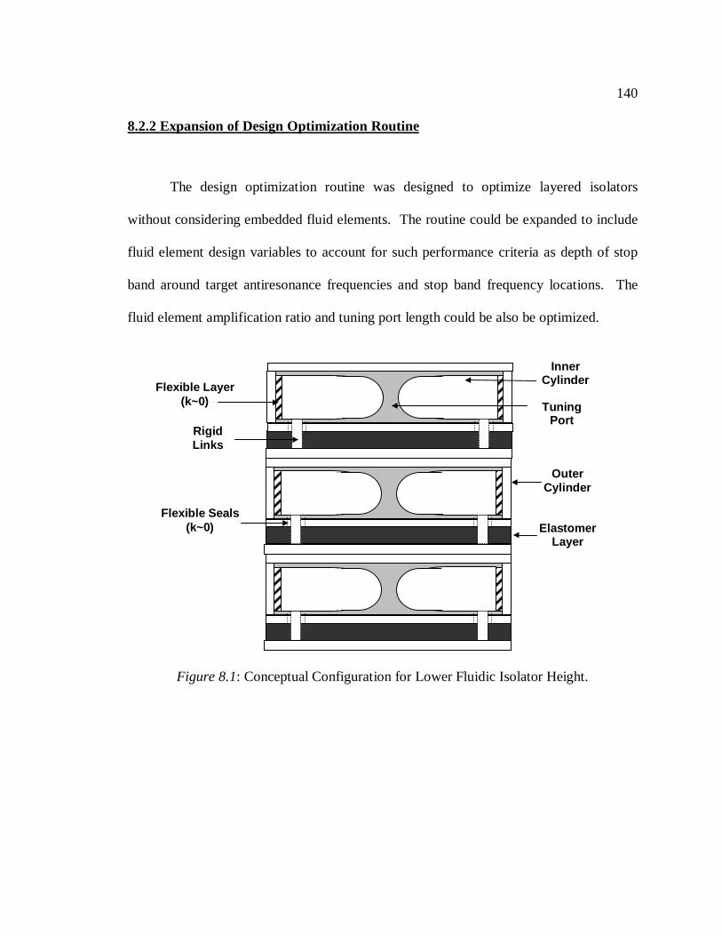
140
8.2.2 Expansion of Design Optimization Routine
The design optimization routine was designed to optimize layered isolators
without considering embedded fluid elements. The routine could be expanded to include
fluid element design variables to account for such performance criteria as depth of stop
band around target antiresonance frequencies and stop band frequency locations. The
fluid element amplification ratio and tuning port length could be also be optimized.
Figure 8.1: Conceptual Configuration for Lower Fluidic Isolator Height.
InnerCylinder
OuterCylinder
Flexible Seals(k~0) Elastomer
Layer
RigidLinks
TuningPort
Flexible Layer(k~0)

141
8.2.3 Stiffness and Fatigue Testing.
Two of the most important performance characteristics of layered helicopter
gearbox isolators would be their axial stiffness and fatigue limits. Stiffness testing of
layered specimens should be conducted to verify the actual quasi-static stiffness is as
predicted using elastomer shape factor. The effect of precompression on isolator
stiffness, briefly discussed in Appendix F, should be examined more thoroughly. Also, a
means to constrain or perhaps stiffen the isolators in the lateral direction should be
considered. A more rigorous investigation into fatigue limits should be pursued, as well.
Both of these tasks should probably be performed in coordination with the Lord
Corporation, because of its extensive knowledge of elastomer behavior.
8.2.4 Conceptual Strut/Isolator Configuration
As the only rigid connection between the fuselage and gearbox in many
helicopters, support struts carry the entire weight of the fuselage in addition to any forces
developed during transitional flight conditions. These forces would primarily result in a
tensile load in the strut. When not in flight, however, these struts support the entire
weight of the gearbox and rotor, and thus are subjected to compressive loads. Therefore,
this change in force must be considered if an isolator is to be placed in series between the
fuselage and gearbox.

142
In Figure 8.2.a, a conceptual gearbox support strut with an embedded layered
isolator is illustrated. The design consists of a set of outer and inner cylindrical sections,
with the isolator embedded in the inner cylinder. The design is such, that if either a
tensile or compressive load is applied to the strut, the entire magnitude of the force is
transferred through the isolator as a compressive force. Because failure of a layered
isolator in tension would rely on the integrity of an elastomer-metal bond alone, aircraft
safety design guidelines and certification would require that such an isolator remain in
compression.

143
In Figure 8.2.b , the load path for a compressive load is highlighted through the
strut. The schematic illustrates how the load would travel through the top portion of the
outer cylinder, then would be transferred through the isolator, and finally would pass
Figure 8.2: Conceptual Strut Configuration to Ensure Compressive Loads on EmbeddedLayered Isolator.
Load Path inCompression
Load Pathin Tension
ConceptualGearbox SupportStrut with Layered
Isolator
DisplacementStops
InnerCylinder
OuterCylinder Isolator in
Compression
(a) (b) (c)

144
through the lower portion of the inner cylinder. Figure 8.2.c illustrates the load path for
when tensile load is applied to the strut. The load will again be passed through the upper
portion of the outer cylinder. Next, the load will be transferred through bolts, which will
serve to compress the isolator, and are connected to the opposite end of the isolator.
Finally, the load will travel through the entire length of the inner cylinder. In this way,
regardless of the sign of the load on the strut, and compressive load will be applied to the
isolator.
8.2.5 Construction of a Demonstration Layered Helicopter Gearbox Isolator
Upon completion of the above recommendations, a proof-of-concept gearbox
isolator/mounting should be designed, fabricated, and tested to demonstrate the efficacy
using layered isolators for helicopter gearbox isolation. The design should satisfy all
mounting performance criteria of a specific helicopter model.
8.2.6 Semi-active Tuning of Fluid Isolator Inner Diameter
A long term research task should be the development of means to semi-actively
tune layered gearbox isolators. As reported in the first chapter of this thesis, irritating
high-frequency gearbox noise is tonal in nature. Because various troublesome tones may
become more or less prominent in changing flight conditions, providing a means to semi-
actively tune a fluidic isolator would allow for better overall interior noise control.

145
In Figure 8.3, a conceptual cell configuration is shown involving a SMA (shape
memory alloy) wire and a contractable inner cylinder. When current is passed through
the SMA wire, it would be heated and consequently would contract axially. By attaching
a coiled wire to the contractable inner cylinder, a given cell could be semi-actively tuned
so that the absorber frequencies would coincide with whichever tones are most prominent
in the gearbox noise signature. For example, if the wire is coiled 10 times at a diameter
of 6 cm, then the total wire length would be about 180 cm. Assuming a maximum strain
of 5%, heating of the wire would cause nearly a 10 cm decrease in the inner area
circumference. This significant change in inner diameter would translate into dramatic
changes in amplification ratio, R, and thus large changes in tuning frequency. Although
SMA wires would require little power and would provide a means to tune a fluidic
isolator, any suitable electroactive material incorporated appropriately could be
envisioned to semi-actively tune the inner cylinders.
146
Figure 8.3: Conceptual Contractable Inner Diameter Using SMA Wires for Semi-activelyTuning Fluidic Isolators.
ContinuousSMA wire
OuterCylinder
ContractableInner
CylinderFlexible
SealsFixed Wire
Ends
FlexibleOverlapping
Sleeve

BIBLIOGRAPHY
1. Snowden, J.C., Vibration Isolation: Use and Characterization, Applied Research
Laboratory, The Pennsylvania State University, Sponsored by the National
Bureau of Standards, pp. 25-37, May 1979.
2. Szefi, J.T., Smith, E.C., Lesieutre, G.A., “Analysis and Design of High Frequency
Periodically Layered Isolators in Compression,” ,” 41st Structures, Structural
Dynamics and Materials Conference, April 3-6, 2000, Atlanta, GA, 2000, pp. 306-
321, 2000.
3. Szefi, J.T., Smith, E.C. and Lesieutre, G.A., “Formulation and Validation of a
Ritz-Based Analytical Model for Design of Periodically-Layered Isolators in
Compression,” 42st Structures, Structural Dynamics and Materials Conference,
Seattle, WA, April 16-19, 2001, pp. 3690-3704, 2001.
4. Ghosh, A.K., “Periodically Layered Composites for Attenuation of Dynamic
Loads,” Nuclear Engineering and Design, Vol. 84, pp. 53-58, 1985.

148
5. Sackman, J.L., Kelly, J.M. and Javid, A.E., “Layered Notch Filter for High
Frequency Dynamic Isolation,” ASME, Pressure Vessels and Piping Conference
and Exhibition, Chicago, IL, Vol. 113, pp. 55-64, 1986.
6. Sackman, J.L., Kelly, J.M. and Javid, A.E., “A Layered Notch Filter for High-
Frequency Dynamic Isolation,” Journal of Pressure Vessel Technology, Vol. 111,
pp. 17-24, 1989.
7. Mead, D.J., Passive Vibration Control, Chichester, N.Y.: Wiley, 1999.
8. Gent, A.N., Meinecke, E.A. “Compression, Bending, and Shear of Bonded
Rubber Blocks,” Poly. Eng. and Science, Vol. 10, no. 1, pp. 48-53, 1970.
9. Sheridan, P.M., James, F.O., Miller, T.S., “Design of Components” in Gent, A.N.,
Ed., Engineering with Rubber: How to Design Rubber Components, Hanser
Publishers, Munich, pp. 214-215, 1992.
10. Pollard, J.S., “Helicopter Gear Noise and its Transmission to the Cabin,” 3rd
European Rotorcraft and Powered Lift Aircraft Forum, Aix-en-Provence, France,
pp. 52.1-52.10, 1977.
11. Coy, J.J., Handschuh, R.F., Lewicki, D.G., Huff, R.G., Krejsa, E.A., Karchmer,
A.M. “Identification and Proposed Control of Helicopter Transmission Noise at
the Source,” NASA/Army Rotorcraft Technology. v.1 Aerodynamics, and
Dynamics and Aeroelasticity, Moffett Field, CA, pp. 1045-1065, 1988.

149
12. D’Ambra, F., Leverton, J.W., “Design Implications of Recent Gearbox Noise and
Vibration Studies,” 4th European Rotorcraft and Powered Lift Aircraft Forum, pp.
56.1-56.22, 1978.
13. Yoerkie, C.A., Moore, J.A., “Statistical Energy Analysis Modeling of Helicopter
Cabin Noise,” 39th Annual Forum of the American Helicopter Society, pp. 458-
471, 1983.
14. Yoerkie, C.A, Moore, J.A., Manning, J.E., “Development of Rotorcraft Interior
Noise Control Concepts, Phase I: Definition Study,” NASA Contractor Report
166101, 1983.
15. Yoerkie, C.A., Gintoli, P.J., Moore, J.A., “Development of Rotorcraft Interior
Noise Control Concepts, Phase II: Full Scale Testing,” NASA Contractor Report
172594, 1986.
16. Yoerkie, C.A., Gintoli, P.J., Ingraham, S.T., Moore, J.A., “Development of
Rotorcraft Interior Noise Control Concepts, Phase III: Development of Noise
Control Concepts,” NASA Contractor Report 178172, 1987.
17. Yoerkie, C.A., Ingraham, S.T., Moore, J.A., “Treated Cabin Acoustic Prediction
using Statistical Energy Analysis,” 43rd Annual Forum and Technology Display of
the American Helicopter Society, St. Louis, Missouri, pp. 461-468, 1987.

150
18. Morgan, H.G., Pao, S.P., Powell, C.A., “Recent Langley Helicopter Acoustics
Contributions,” NASA/Army Rotorcraft Technology v.1 Aerodynamics, and
Dynamics and Aeroelasticity, Moffett Field, CA, pp. 1003-1044, 1988.
19. O’Connell, J., “Predicting Rotorcraft Transmission Noise,” 48th Forum of the
American Helicopter Society, pp. 919-929, 1992.
20. Mathur, G.P., Manning, J.E., “Analytical Prediction and Flight Test Evaluation of
Bell ACAP Helicopter Cabin Noise,” 44th Forum of the American Helicopter
Society, pp. 719-729, 1988.
21. Brennan, M.J., Pinnington, R.J., Elliott, S.J., “Mechanisms of Noise Transmission
through Helicopter Gearbox Support Struts,” Journal of Vibrations and Acoustics,
Vol. 116, pp. 548-554, 1994.
22. Brennan, M.J., Elliott, S.J., Heron, K.H., “Noise Propagation through Helicopter
Support Struts – An Experimental Study,” Journal of Vibration and Acoustics,
Vol. 120, pp. 695-704, 1998.
23. Ohlrich, M., “Terminal Source Power for Predicting Structureborne Sound
Transmission from a Main Gearbox to a Helicopter Fuselage,” Proceedings of
Internoise 1995, pp. 555-558, 1995.
24. Marze, H.J., D’Ambra, F.N., “Helicopter Internal Noise Treatment: Recent
Methodologies and Practical Applications,” 11th European Rotorcraft Forum:
Paper No. 10, London, England, pp. 10.1-10.13, 1985.
151
25. Levine, L.S., “Reducing the Cost Impact of Helicopter Internal Noise Control,”
36th Annual Forum of the American Helicopter Society, pp. 80.59.1-80.59.9,
1980.
26. Owen, S., Woodward, M.C.A., Pollard, J.S. “Demonstration of Potential
Acoustic Gains from Conventional Cabin Soundproofing Treatments,” 4th
European Rotorcraft and Powered Lift Aircraft Forum: Paper No. 60, Stresa,
Italy, 1978.
27. Dorling, C.M., Eatwell, G.P., Hutchins, S.M., Ross, C.F., Sutcliffe, S.G.C.,
“Demonstration of Active Noise Reduction in an Aircraft Cabin,” Journal of
Sound and Vibration, Vol. 128, no. 2, pp. 358-360, 1989.
28. Elliott, S.J., Nelson, P.A., Stothers, I.M., Boucher, C.C., “Preliminary Results of
In-flight Experiments on the Active Control of Propeller-Induced Cabin Noise,”
Journal of Sound and Vibration, Vol. 128, pp. 355-357, 1989.
29. Jolly, M.R., Norris, M.A., Rossetti, D.J., “Adaptive Control of Helicopter Cabin
Noise,” Proceedings of the ASME Dynamic Systems and Control Division, Vol.
57-2, pp. 837-848, 1995.
30. Millott, T.A., Welsh, W.A., Yoerkie, C.A., MacMartin, D.G., Davis, M.W.,
“Flight Test of Active Gear-Mesh Noise Control on the S-76 Aircraft,” 54th
Annual Forum of the American Helicopter Society, pp. 241-249, 1998.
152
31. Grewal, A., Pavel, L., Zimcik, D.G., Leigh, B. Xu, W., “Application of
Feedforward and Feedback Structural Control for Aircraft Cabin Noise
Reduction,” Proceedings of the 1998 39th AIAA/ASME/ASCE/AHS/ASC
Structures, Structural Dynamics, and Materials Conference and Exhibit and
AIAA/ASME/AHS Adaptive Structures Forum, pp. 2265-2275, 1998.
32. Grewal, A., Zimcik, D.G., Leigh, B., “Feedforward Piezoelectric Structural
Control: An Application to Aircraft Cabin Noise Reduction,” Journal of Aircraft,
Vol. 38, no. 1, pp.164-173, 2001.
33. Hirsch, S.M., Jayachandran, V., Sun, J.Q., “Structural-Acoustic Control for
Quieter Aircraft Interior-Smart Trim Technology,” Composite Structures, Vol. 42,
pp. 189-202, 1998.
34. Palumbo, D., Cabell, R., Sullivan, B., “Flight Test of Active Structural Acoustic
Noise Control System,” Journal of Aircraft, Vol. 38, no. 2, pp. 277-284, 2001.
35. Sun, J.Q., Hirsch, S.M., Proceedings of SPIE - The International Society for
Optical Engineering, Vol. 3041, pp. 839-845, 1997.
36. O’Connell, J., Mathur, G., JanakiRam, R. Johnson, M., Rosetti, D.J., “Helicopter
Cabin Noise Reduction Using Active Structural Acoustic Control,” 57th Annual
Forum of the American Helicopter Society, 2001.

153
37. Fuller, C.R., Snyder, S.D., Hansen, C.H., Silcox, R.J., “Active Control of Interior
Noise in Model Aircraft Fuselages Using Piezoceramic Actuators,” AIAA
Journal, Vol. 30, no. 11, pp. 2613-2617, 1992.
38. Sun, J.Q., Norris, M.A., Rossetti, D.J., Highfill, J.H., “Distributed Piezoelectric
Actuators for Shell Interior Noise Control,” Journal of Vibration and Acoustics,
Vol. 118, pp. 676-681, 1996.
39. Gembler, W., Schweitzer, H., “Helicopter Interior Noise Reduction by Active
Gearbox Struts,” 54th Annual Forum of the American Helicopter Society, pp. 216-
229, 1998.
40. Bebesel, M., Maier, R. Hoffmann, F., “Reduction of Interior Noise in Helicopters
by Using Active Gearbox Struts – Results of Flight Tests,” 27th European
Rotorcraft Forum, pp. 1.1-1.8, 2001.
41. Sutton, T.J., Elliott, S.J., Brennan, M.J., “Active Isolation of Multiple Structural
Waves on a Helicopter Gearbox Support Strut,” Journal of Sound and Vibration,
Vol. 205, no. 1, pp. 81-101, 1997.
42. Pelinescu, I., Balachandran, B., “Active Control of Vibration Transmission
through Struts,” Proceedings of SPIE, Vol. 3329, pp. 596-607, 1998.
43. Pelinescu, I., Balachandran, B., “Control of Wave Transmission through Struts,”
Proceedings of the SPIE Conference on Smart Structures and Integrated Systems,
Newport Beach, CA, 80-91, 1999.

154
44. Pelinescu, I., Balachandran, B., “Analytical and Experimental Investigations into
Active Control of Wave Transmission through Gearbox Struts,” Proceedings of
SPIE, Vol. 3985, pp. 76-85, 2000.
45. Pelinescu, I., Balachandran, B., “Analytical Study of Active Control of Wave
Transmission through Cylindrical Struts,” Smart Materials and Structures, 10,
121-136, 2001a.
46. Pelinescu, I., Balachandran, B., ”Experimental Study of Active Control of Wave
Transmission through Hollow Cylindrical Struts,” Proceedings of SPIE, Vol.
4327, pp. 1-12, 2001b.
47. Mahapatra, D.R., Gopalakrishnan, S., Balachandran, B., “Active Feedback
Control of Multiple Waves in Helicopter Gearbox Support Struts,” Smart
Materials and Structures, Vol. 10, pp. 1046-1058, 2001.
48. Ortel, D.J., Balachandran, B., “Control of Flexural Wave Transmission through
Struts,” Proceedings of the SPIE Conference on Smart Structures and Integrated
Systems, Newport Beach, CA, pp. 567-577, 1999.
49. Vincent, Phil. Mag.,Vol. 46, pp. 537, 1898.
50. Lawry, M.H., I-DEAS� Master Series, Student Guide, Structural Dynamics
Research Corporation, 1997.

155
51. Heyliger, P.R. “Axisymmetric Free Vibrations of Finite Anisotropic Cylinders,”
Journal of Sound and Vibration, Vol. 124, pp. 507-520, 1991.
52. Hurty, W.C., “Dynamic Analysis of Structural Systems Using Component
Modes,” AIAA Journal, Vol. 3, pp. 678-685, 1965.
53. Welsh, W.A., Von Hardenberg, P.C.;Von Hardenberg, P.W., Staple, A.E., “Test
and Evaluation of Fuselage Vibration Utilizing Active Control of Structural
Response,” 46th Annual Forum Proceedings of the American Helicopter Society.
Part 1 (of 2), May 21-23 1990, Washington, DC, USA, pp. 21-37, 1990.
54. Smith, M.R., Redinger, W.S., “The Model 427 Pylon Isolation System,” 55th
Annual Forum of the American Helicopter Society, Montreal, Quebec, Canada,
1999.
55. Donguy, P., “Development of a Helicopter Rotor Hub Elastomeric Bearing,”
Journal of Aircraft, Vol. 17, No. 5, pp. 346-350, 1980.
56. Long, J.E. , Bearings in Structural Engineering, NY, New York, Halsted Press,
1974.
57. Mertz, D.R., Kulicki, J.M., “Bridge design by the AASHTO LRFD Bridge Design
Specifications,” Structures Congress - Proceedings, v1, 1996, Building an
International Community of Structural Engineers, Proceedings of the 14th
Structures Congress. Part 1 (of 2), Chicago, IL, USA, pp. 1-8, 1996.

156
58. Roeder, C.W., Stanton, J.F., “Elastomeric Bearings: State-of-the-Art,” Journal of
Structural Engineering, Vol. 109, No. 12, pp. 2853-2871, 1982.
59. Roeder, C.W., Stanton, J.F., Taylor, A.W., “Fatigue of Steel-Reinforced
Elastomeric Bearings,” Journal of Structural Engineering, Vol. 116, No. 2, pp.
407-426, 1987a.
60. Roeder, C.W., Stanton, J.F., Taylor, A.W., “Performance of Elastomeric
Bearings,” National Cooperative Highway Research Program Report, Oct, 1987,
100p, 1987b.
61. Roeder, C.W., Stanton, J.F., Feller, T., “Low-Temperature Performance of
Elastomeric Bearings,” Journal of Cold Regions Engineering, Vol 4, No. 3, pp.
113-132, 1990.
62. Roeder, C.W., Stanton, J.F., “State-of-the-Art Elastomeric Bridge Bearing
Design,” ACI Structural Journal, Vol. 88, No. 1, pp. 31-41, 1991.
63. Stanton, J.F., Roeder, C.W., “Elastomeric Bearings: An Overview,” Concrete
International: Design and Construction, Vol. 14, No. 1, pp. 41-46, 1992.
64. Stevenson, A., Campion, R.P., “Durability” in Gent, A.N., Ed., Engineering with
Rubber: How to Design Rubber Components, Hanser Publishers, Munich, pp.
179-183, 1992.

157
65. Seeley, C.E., Chattopadhyay, A., “Development of a Hybrid Technique for
Continuous/Discrete Optimization,” Proc. 6th Annual AIAA/NASA/ISSMO Symp.
On Multidisciplinary Analysis and Optimization (Bellevue, WA), 1996, pp. 1430-
1440, 1996.
66. Carlson, J.D., Jolly, M.R., “MR Fluid, Foam, and Elastomer Devices,”
Mechatronics, Vol. 10, pp. 555-569, 2000.
67. Ginder, J.M., Nichols, M.E., Elie, L.D., Tardiff, J.L., “Magnetorheological
Elastomers: Properties and Applications,” Proceedings of SPIE, Vol. 3675, pp.
131-138, 1999.
68. Ginder, J.M., Nichols, M.E., Elie, L.D., Clark, S.M., “Controllable-Stiffness
Components Based on Magnetorheological Elastomers,” Proceedings of SPIE,
Vol. 3985, pp. 418-425, 2000.
69. Jolly, M.R., Carlson, J.D., Munoz, B.C., Bullions, T.A., “The
Magnetoviscoelastic Response of Elastomer Composites Consisting of Ferrous
Particles Embedded in a Polymer Matrix,” Journal of Intelligent Material Systems
and Structures, Vol.7, pp. 613-622, 1996a.
70. Jolly, M.R., Carlson, J.D., Munoz, B.C., “A Model of the Behaviour of
Magnetorheological Materials,” Smart Materials and Structures, Vol.5, No.5, pp.
607-614, 1996b.

158
71. Davis, C., "A Tunable Piezoceramic Vibration Absorber," Ph. D. Thesis, Dept. of
Aersp. Eng., The Pennsylvania State University, University Park, PA, 1997.
72. Davis, C. L., G.A. Lesieutre, "Actively tuned Solid-State Vibration Absorber
Using Capacitive Shunting of Piezoelectric Stiffness", Journal of Sound and
Vibration, Vol. 232, No. 3, pp. 601-617, 2000.
73. Dozor, D.M., Jagannathan, S., Gerver, M.J., Fenn, R.C., Logan, D.M., Berry, J.R.,
“High Force to Volume Terfenol-D Reaction Mass Actuator: Modeling and
Design,” Proceeding of SPIE, Vol. 2717, pp. 576-586, 1996.
74. Johnson, W., “Self-tuning Regulators for Multicyclic Control of Helicopter
Vibration,” NASA Technical Paper 1996, March 1982.
75. Anusonti-Inthra, Phuriwat, “Semi-Active Control of Helicopter Vibration Using
Controllable Stiffness and Damping Devices,” Ph. D. Thesis, Dept. of Aersp.
Eng., The Pennsylvania State University, University Park, PA, 2002.
76. McGuire, D.P., “Fluidlastic® Dampers and Isolators for Vibration Control in
Helicopters,” 50th Annual Forum of the American Helicopter Society, pp. 295-
303, 1994.
77. Ungar, E.E., Dietrich, C.W., “High Frequency Vibration Isolation,” Journal of
Sound and Vibration, Vol. 4, pp. 224-241, 1961.

159
78. Molloy, C.T., Mechanical Impedance Methods, “Section 4: Four Pole Parameters
in Vibration Analysis,” ed. by R. Plunkett, New York: ASME, 1958.
79. Sjoberg, Mattias, “On Dynamic Properties of Rubber Isolators,” Ph.D. Thesis,
Dept. of Vehicle Engineering, Royal Institute of Technology, Stockholm,
Sweden, 2002.
80. Scobbo, J.J., “Characterization of Filled Elastomers by Dynamic Strain
Amplification at High Frequencies,” Polymer Testing, Vol 9, No. 6, pp.405-420,
1990.
81. Kari, L., Sjoberg, M., “Temperature Dependent Stiffness of a Precompressed
Rubber Isolator in the Audible Frequency Range,” Manuscript submitted to
International Journal of Solids and Structures, 2002.
82. Kari, L., “Dynamic Transfer Stiffness Measurements of Vibration Isolators In
theAudible Frequency Range,” J. of Noise Control Engineering, Vol. 49, No. 2,
pp. 88-102, 2001.
83. DeJong, R.G., Ermer, G.E., Paydenkar, C.S., Remtema, T.M., “High Frequency
Dynamic Properties of Rubber Isolation Elements, Proceedings – National
Conference on Noise Control Engineering, Part 1 (of 3), Apr 5-9, 1998, Ypsilanti,
MI, USA.

Appendix A
DERIVATION OF THE EQUATIONS OF MOTION FOR A
VIBRATING CYLINDER AS PRESENTED BY HEYLIGER [51]
The following derivation accompanies the discussion in of the development of an
approximation method for layered isolators presented in Chapter 2. It is adapted from
Heyliger’s original derivation presented in Ref. 51.
The non-zero strain components for axisymmetric motion can be written (in
cylindrical coordinates) as
1 ,rr
u
rε ε ∂= =
∂ 2
u
rθθε ε= = , 3 ,zz
w
zε ε ∂= =
∂ 5 rz
w u
r zε ε ∂ ∂= = +
∂ ∂( A.1 )
Hamiltion’s principle is then used to obtain the equations of motion, which can be
expressed as
{ } 2 21 1 2 2 3 3 5 5
0 0
10 ( )
2
t t
V V
dVdt u w dVdtσ δε σ δε σ δε σ δε δ ρ= − + + + + +� � � � � � ( A.2 )

161
where V is the volume of the cylinder, /u u t= ∂ ∂� , t is time, ρ is the density of the
material, σι is the ith stress component, with the subscript notation matching that of the
strains in Eq. (A.1) , and δ is the variational operator.
In this derivation, there are no external forces and the cylinder is assumed to be
stress free. The constitutive relations are written in matrix form as
11 12 131
12 22 232
3 13 23 33
4 55
000
0 0 0
rr rr
zz zz
rz rz
C C CC C CC C C
C
θθ θθ
σ σ εσ σ εσ σ εσ σ γ
� �� � � � � �� �� � � � � �
= = � �� � � � � �� �� � � � � �� � � �
( A.3 )
For numerical calculations, it is convenient to non-dimensionalize the cylinder
geometry by mapping the original cylinder to a cylinder with a radius and half-height of 1
using the transformations
/R r L= , / (1/ ) /rr L R∂ ∂ = ∂ ∂
/ zZ z L= / (1/ ) /zz L Z∂ ∂ = ∂ ∂( A.4 )
Here Lr is the radius of the cylinder, Lz = h/2, and h is the total height of the cylinder, as
shown in Figure A.1.

162
The domain of integration is also transformed and can be rewritten as
2r zdV rdrd dz RL L dRd dZθ θ= = ( A.5 )
For convenience, it has been assumed that this transformation has been completed, but
the upper-case nomenclature is dropped for the transformed coordinates.
The variational form of the governing equations can be derived by substituting
Eqs. (A.1) and (A.3) into Eq. (A.2). The variational form of the equations of motion is
Figure A.1: Geometry of Cylinder
2Lr
2Lz
z
r

163
11 12 122 2 2
1 10
r r rV
C u u C u C uu u
L r r r L r r L r
δ δδ� ∂ ∂ ∂ ∂= + +� ∂ ∂ ∂ ∂�
�
13 13 231 1
r z r z r z
C C Cu w w wu u
r L L r z L L z r L L z
δ δδ∂ ∂ ∂ ∂+ + +∂ ∂ ∂ ∂
3322552 2 2
1 1 1
r z r z
CC w w w uu u C
r L L z z L r L z
δδ� �∂ ∂ ∂ ∂+ + +� �∂ ∂ ∂ ∂� �
1 1( )
r z
w uu u w w dV
L r L z
δ δ ρ δ δ�� �∂ ∂ �× + + + �� �∂ ∂ �� �
�� ��
( A.6 )
in V. Additionally, by integrating by parts the boundary conditions can be found to be
specify u or
11 12 13 r
u wC C u C n
r z
∂ ∂� �+ +� �∂ ∂� �55 z rr r rz z
w uC n n n
r zσ σ∂ ∂� �+ + = +� �∂ ∂� �
( A.7 )
specify v or
55 13 23 33
1r z
w u u wC n C C u C n
r z r r z
∂ ∂ ∂ ∂� � � �+ + + +� � � �∂ ∂ ∂ ∂� � � �rz r zz zn nσ σ= + ( A.8 )
on Γ. Here Γ represents the surface of the cylinder , and nr and nz are the components of
the outward unit normal vector to this surface in r and z directions. For this work, u and v
are both specified.

Appendix B
EXPLICIT FORMS OF [M] AND [K] MATRICES AS REPORTED BY
HEYLIGER [51]
The following matrix definitions accompany the discussion in of the development
of an approximation method for layered isolators presented in Chapter 2, and were
originally presented by Heyliger in Ref. 51. The axisymmetric matrices, [M] and [K], are
explicitly defined for a vibrating isotropic cylinder.
The matrices in the eigenvalue problem can be written as
{ }{ }
{ }{ }
{ }{ }
11 12 112
21 22 22
0000
b bK K Md dK K M
ρω� � � � � �� � � �− =� � � � � �� � � �
� � � � �( B.1 )
Here
11 u uij i j
V
M rdrd dzφ φ θ= � ( B.2 )

165
22 w wij i j
V
M rdrd dzφ φ θ= � ( B.3 )
11 11 122 2
1u uu uj ju ui i
ij j ir rV
C CK
L r r r L r r
φ φφ φ φ φ� � �∂ ∂∂ ∂= + +� � �� �∂ ∂ ∂ ∂� � ��
�
55222 2 2
1uuju u i
i jr z
CCrdrd dz
r L L z z
φφφ φ θ�∂∂+ + �∂ ∂ ��
( B.4 )
12 13 23 551w w wu uj j jui i
ij ir z r z r zV
C C CK
L L r z r L L z L L z r
φ φ φφ φφ� �∂ ∂ ∂∂ ∂= + +� �∂ ∂ ∂ ∂ ∂� �� �
�
21( ) jirdrd dz Kθ× =
( B.5 )
22 33 552 2
w ww wj ji i
ijz r
C CK rdrd dz
L z z L r r
φ φφ φ θ� �∂ ∂∂ ∂= +� �∂ ∂ ∂ ∂� �� �
( B.6 )

Appendix C
MATLAB® CODE: DESIGN OPTIMIZATION FOR LAYERED
ISOLATORS IN COMPRESSION
The following is the MATLAB® code for the design optimization of layered
isolators in compression. The code consists of a main program, and functions ‘initial’,
‘fcomp’, ‘calc3D’, ‘calcaxstiff2’, and ‘calclatstiff2’. Design constraints and objectives
are specified in the function ‘initial’.
Main Program
%%%%%%%%%%%%%%%%%%%%%%%%%%%%%%%%%%%%%%%%%%%%%%%%%%%%%%%%%%%%%%%%%%%%%%%%%%%%%%%%%%%%% "Design of periodically layered isolators in compression using simulated annealing"%% Rotorcraft Center of Excellence% Penn State University% Joseph T. Szefi% [email protected]% 9/1/2003%%%%%%%%%%%%%%%%%%%%%%%%%%%%%%%%%%%%%%%%%%%%%%%%%%%%%%%%%%%%%%%%%%%%%%%%%%%%%%%%%%%%
clear all;close all;
% Grub=x(1);% Gmet=x(2);% rhorub=x(3);% rhomet=x(4);% n=x(5)% trub=x(6);% tmet=(h-n*trub)/n;% d = x(7);% h = x(8);
% Get variable values from 'intial.m'[btarget, etarget, masstarg, alphab, alphae, beta, minaxstiff, maxaxstiff,... minlatstiff, maxlatstiff, maxatten, Grubmin, Grubmax, Gmetmin, Gmetmax, rhorubmin, rhorubmax,... tmetmin, trubmin, rhometmin, rhometmax, nmin, nmax, dmin, dmax, hmin, hmax, elastomer, maxmass,Fcompress] = initial;
% Open output filefid = fopen('compout.m','w');
% Define optimization parameter valuesnvar = 8;eps = 1E-4;epsr = 1E-3;step = 1;
%%%%%%%%%%%%%%%%%%%%%%%%%%%%%%%%%%%%%%%%%%%%%%%%%%%%%%%%%%%%%%%%%%%%%%%%%%%%%%%%%%%%%%%%%%%%%%%%%%%%%%%%%%%%%%%%%%%%%%%%%%%%%%%%%%%%%%%%%%%%%%%%%%%%%%%%%%%%%%%%%%%%%%% The following variables determine the amount of parameter% sampling during optimization.% ntp = overall iterations a given 'temperature'% ncyc = # of variable samplings at a given temperature%

167
% Increasing either will, in general, increase running time, but will also better% ensure that a minimum is found
ntp = 20;ncyc = 10;
%%%%%%%%%%%%%%%%%%%%%%%%%%%%%%%%%%%%%%%%%%%%%%%%%%%%%%%%%%%%%%%%%%%%%%%%%%%%%%%%%%%%%%%%%%%%%%%%%%%%%%%%%%%%%%%%%%%%%%%%%%%%%%%%%%%%%%%%%%%%%%%%%%%%%%%%%%%%%%%%%%%%%%
ntot = 1000000;Irepeat = 10;
% Read intial temperature, reduction parameter, step factorT = 200;rp = 0.6;sf = 2;rs = 0.8;
% Check for number of layer errorsif nmin < 2 fprintf('Error: Check minimum number of layers\n'); fprintf(fid,'Error: Check minimum number of layers\n'); fclose(fid); break;end
if (nmax > 15) fprintf('Error: Check maximum number of layers\n'); fprintf(fid,'Error: Check maximum number of layers\n'); fclose(fid); break;end
if (nmin > nmax) fprintf('Error: Minimum number of layers greater than maximum number of layers\n'); fprintf(fid,'Error: Minimum number of layers greater than maximum number of layers\n'); fclose(fid); break;end
nmin = nmin - .5;nmax = nmax + 0.4999;
% Define min and maxxmin(1,1) = Grubmin;xmin(1,2) = Gmetmin;xmin(1,3) = rhorubmin;xmin(1,4) = rhometmin;xmin(1,5) = nmin;xmin(1,6) = trubmin;xmin(1,7) = dmin;xmin(1,8) = hmin;
xmax(1,1) = Grubmax;xmax(1,2) = Gmetmax;xmax(1,3) = rhorubmax;xmax(1,4) = rhometmax;xmax(1,5) = nmax;xmax(1,7) = dmax;xmax(1,8) = hmax;
for count = 1:nvar if count==6 x(5) = round(x(5)); xmax(1,6)=(hmax-tmetmin*x(5))/x(5); end x(count) = xmin(count) + rand(1)*(xmax(count)-xmin(count));end
xopt = x;xs = x;for c = 1:nvar, st(c) = step*(xmax(c)-xmin(c)); ar(c) = 1;endnfv = 1;
n = xs(5);h = xs(8);
tmet = (h-xs(6)*xs(5))/xs(5);trub = xs(6);
if (tmet < tmetmin)|(tmet < 0) xs(6)=(h-tmetmin*n)/n;end
if (trub < trubmin) xs(6)=trubmin;end
F = fcomp(xs, btarget, etarget, masstarg, alphab, alphae, beta,... minaxstiff, maxaxstiff, minlatstiff, maxlatstiff, maxatten, maxmass,Fcompress);
Fmin = F;ict = 0;Fold = F;cr = 0;firsttry = 1;x=xs;while (1 > 0) d = x(7); h = x(8); axstiff = calcaxstiff2(x); latstiff = calclatstiff2(x); n=x(5); mass = n*d^2*pi/4*((h-n*x(6))/n*x(4) + x(6)*x(3)); atten = 0; SF = d/4/x(6); minSF = Fcompress/(d^2*pi/4)/2/x(1); [threedstart,threedend] = calc3D(x); fprintf('-------------------------------------------------------------------------------------------------------------------------\n'); fprintf(' Iteration'); fprintf(fid,'-------------------------------------------------------------------------------------------------------------------------\n'); fprintf(fid,' Iteration'); if firsttry == 1 fprintf(' 0 | %6.0f | %6.0f |\n', btarget, etarget); fprintf(fid,' 0 | %6.0f | %6.0f |\n', btarget, etarget); firsttry = 0; else if cr < 10 fprintf(' %0.0f | %6.0f | %6.0f |\n', cr, btarget, etarget);

168
fprintf(fid,' %0.0f | %6.0f | %6.0f |\n', cr, btarget, etarget); else fprintf(' %0.0f | %6.0f | %6.0f |\n', cr, btarget, etarget); fprintf(fid,' %0.0f | %6.0f | %6.0f |\n', cr, btarget, etarget); end end fprintf('-------------------------------------------------------------------------------------------------------------------------\n'); fprintf('| # of cells | Elas. thick. | Met. thick. | Beg. Freq. | End Freq. | Elas. rho | Met. rho | Isolator Mass \n'); fprintf('| | (cm) | (cm) | (Hz) | (Hz) | (kg/m^3) | (kg/m^3) | (kg)\n'); fprintf('-------------------------------------------------------------------------------------------------------------------------\n'); fprintf('%8.0f %15.3f %16.3f %14.0f %14.0f %13.0f %13.0f %14.2f\n',n, (x(6)*100),((h-x(5)*x(6))/x(5)*100), threedstart,threedend,x(3),x(4),mass); fprintf('=========================================================================================================================\n'); fprintf('| G Elas. | G Met. | Axial Stiff. | Lat. Stiff. | d | h | S.F. | min. S.F. \n'); fprintf('| (MPa) | (GPa) | (MN/m) | (MN/m) | (cm) | (cm) | | \n'); fprintf('-------------------------------------------------------------------------------------------------------------------------\n'); fprintf('%8.2f %16.2f %16.2f %14.2f %13.2f %14.2f %15.2f %14.2f\n',(x(1)/1e6),(x(2)/1e9),(axstiff/1e6),(latstiff/1e6),d*100,h*100,SF,minSF); fprintf('\n'); fprintf(fid,'-------------------------------------------------------------------------------------------------------------------------\n'); fprintf(fid,'| # of cells | Elas. thick. | Met. thick. | Beg. Freq. | End Freq. | Elas. rho | Met. rho | Isolator Mass \n'); fprintf(fid,'| | (cm) | (cm) | (Hz) | (Hz) | (kg/m^3) | (kg/m^3) | (kg)\n'); fprintf(fid,'-------------------------------------------------------------------------------------------------------------------------\n'); fprintf(fid,'%8.0f %15.3f %16.3f %14.0f %14.0f %13.0f %13.0f %14.2f\n',n, (x(6)*100),((h-x(5)*x(6))/x(5)*100), threedstart,threedend,x(3),x(4),mass); fprintf(fid,'=========================================================================================================================\n'); fprintf(fid,'| G Elas. | G Met. | Axial Stiff. | Lat. Stiff. | d | h | S.F. | min. S.F. \n'); fprintf(fid,'| (MPa) | (GPa) | (MN/m) | (MN/m) | (cm) | (cm) | | \n'); fprintf(fid,'-------------------------------------------------------------------------------------------------------------------------\n'); fprintf(fid,'%8.2f %16.2f %16.2f %14.2f %13.2f %14.2f %15.2f%14.2f\n',(x(1)/1e6),(x(2)/1e9),(axstiff/1e6),(latstiff/1e6),d*100,h*100,SF,minSF); fprintf(fid,'\n'); cr = cr + 1; track(cr,1:8) = x; track(cr,9) = (h-x(5)*x(6))/x(5); track(cr,10) = F; for itp = 1:ntp,
for icyc = 1:ncyc,
for ih = 1:nvar,
xs(ih) = x(ih) + (2*rand(1)-1) * st(ih);
if ih==5 xs(5) = round(xs(5)); end
if ih==6 xmax(1,6)=(h-tmetmin*xs(5))/xs(5); end
if (xs(ih) < xmin(ih)) | (xs(ih) > xmax(ih))
xs(ih) = xmin(ih) + rand(1) * (xmax(ih)-xmin(ih));
% Round n to nearest variable if ih==5 xs(5) = round(xs(5)); xmax(1,6) = (hmax-tmetmin*xs(5))/xs(5); oldnumofcells = xs(5); end end
n = xs(5); h = xs(8);
%xs(6) = .0062;
tmet = (h-xs(6)*xs(5))/xs(5); trub = xs(6);
%Make sure that thicknesses are positive
if (tmet < tmetmin) | (tmet < 0) xs(6)=(h-tmetmin*n)/n; end
if (trub < trubmin) xs(6)=trubmin; end
Fs = fcomp(xs, btarget, etarget, masstarg, alphab, alphae, beta,... minaxstiff, maxaxstiff, minlatstiff, maxlatstiff, maxatten, maxmass,Fcompress);
nfv = nfv + 1; if Fs <= F; %Point is accepted %fprintf('\nLower Point Accepted\n'); x(ih) = xs(ih); F = Fs; if Fs < Fmin %Set to minimum for c2 = 1:nvar, xopt(c2) = xs(c2); end Fmin = Fs; end else %Apply Metropolis criterion for acceptance P = exp((F-Fs)/T); if rand(1) < P x(ih) = xs(ih); F = Fs; else %Rejection of a point xs(ih) = x(ih); ar(ih) = ar(ih) - 1/ncyc; end end end end
%Adjust step size so half of points are accepted for c3 = 1:nvar, if ar(c3) > 0.6 st(c3) = st(c3)*(1+sf*(ar(c3)-0.6)/0.4); else if ar(c3) < 0.4 st(c3) = st(c3)/(1+sf*(0.4-ar(c3))/0.4); end end if st(c3) > (xmin(c3) - xmax(c3)) st(c3) = xmin(c3) - xmax(c3);

169
end ar(c3) = 1; end end
%Acceptance Criterion Ftol = eps + epsr*abs(Fmin); if (Fmin <= Fold) & (Fold-Fmin < Ftol) ict = ict+1; if ict >= Irepeat fprintf('\n\nExit Loop by Consectutive Minima\n\n'); fprintf(fid,'\n\nExit Loop by Consectutive Minima\n\n'); break; end else ict = 0; end if nfv > ntot fprintf('\n\nExit Loop by Too Many Function Evaluations\n\n'); fprintf(fid,'\n\nExit Loop by Too Many Function Evaluations\n\n'); break; end %Reduce the Temperature for the Next Iteration T = rp*T; st = rs*st; x = xopt; F = Fmin; Fold = F;endx = xopt;c = [1:1:size(track,1)];d = x(7);h = x(8);axstiff = calcaxstiff2(x);latstiff = calclatstiff2(x);n=x(5);mass = n*d^2*pi/4*((h-n*x(6))/n*x(4) + x(6)*x(3));atten = 0;SF = d/4/x(6);minSF = Fcompress/(d^2*pi/4)/2/x(1);[threedstart, threedend] = calc3D(x);fprintf('-------------------------------------------------------------------------------------------------------------------------\n');fprintf(' Optimizied Design');fprintf(fid,'-------------------------------------------------------------------------------------------------------------------------\n');fprintf(fid,' Optimized Design');fprintf(' | %6.0f | %6.0f |\n', btarget, etarget);fprintf(fid,' | %6.0f | %6.0f |\n', btarget, etarget);fprintf('-------------------------------------------------------------------------------------------------------------------------\n');fprintf('| # of cells | Elas. thick. | Met. thick. | Beg. Freq. | End Freq. | Elas. rho | Met. rho | Isolator Mass \n');fprintf('| | (cm) | (cm) | (Hz) | (Hz) | (kg/m^3) | (kg/m^3) | (kg)\n');fprintf('-------------------------------------------------------------------------------------------------------------------------\n');fprintf('%8.0f %15.3f %16.3f %14.0f %14.0f %13.0f %13.0f %14.2f\n',n, (x(6)*100),((h-x(5)*x(6))/x(5)*100), threedstart,threedend,x(3),x(4),mass);fprintf('=========================================================================================================================\n');fprintf('| G Elas. | G Met. | Axial Stiff. | Lat. Stiff. | d | h | S.F. | min. S.F. \n');fprintf('| (MPa) | (GPa) | (MN/m) | (MN/m) | (cm) | (cm) | | \n');fprintf('-------------------------------------------------------------------------------------------------------------------------\n');fprintf('%8.2f %16.2f %16.2f %14.2f %13.2f %14.2f %15.2f %14.2f\n',(x(1)/1e6),(x(2)/1e9),(axstiff/1e6),(latstiff/1e6),d*100,h*100,SF,minSF);fprintf('\n');fprintf(fid,'-------------------------------------------------------------------------------------------------------------------------\n');fprintf(fid,'| # of cells | Elas. thick. | Met. thick. | Beg. Freq. | End Freq. | Elas. rho | Met. rho | Isolator Mass \n');fprintf(fid,'| | (cm) | (cm) | (Hz) | (Hz) | (kg/m^3) | (kg/m^3) | (kg)\n');fprintf(fid,'-------------------------------------------------------------------------------------------------------------------------\n');fprintf(fid,'%8.0f %15.3f %16.3f %14.0f %14.0f %13.0f %13.0f %14.2f\n',n, (x(6)*100),((h-x(5)*x(6))/x(5)*100), threedstart,threedend,x(3),x(4),mass);fprintf(fid,'=========================================================================================================================\n');fprintf(fid,'| G Elas. | G Met. | Axial Stiff. | Lat. Stiff. | d | h | S.F. | min. S.F. \n');fprintf(fid,'| (MPa) | (GPa) | (MN/m) | (MN/m) | (cm) | (cm) | | \n');fprintf(fid,'-------------------------------------------------------------------------------------------------------------------------\n');fprintf(fid,'%8.2f %16.2f %16.2f %14.2f %13.2f %14.2f %15.2f %14.2f\n',(x(1)/1e6),(x(2)/1e9),(axstiff/1e6),(latstiff/1e6),d*100,h*100,SF,minSF);fprintf(fid,'\n');
st = fclose(fid);

170
Function - Initial
function [btarget, etarget, masstarg, alphab, alphae, beta, minaxstiff, maxaxstiff,... minlatstiff, maxlatstiff, maxatten, Grubmin, Grubmax, Gmetmin, Gmetmax, rhorubmin, rhorubmax,... tmetmin, trubmin, rhometmin, rhometmax, nmin, nmax, dmin, dmax, hmin, hmax,elastomer, maxmass, Fcompress] = initial()
%%%%%%%%%%%%%%%%%%%%%%%%%%%%%%%%%%%%%%%%%%%%%%%%%%%%%%%%%%%%%%%%%%%%%%%%%%%%%%%%%%%%% "Design of periodically layered isolators in shear using simulated annealing"%% Rotorcraft Center of Excellence% Penn State University% Joseph T. Szefi% [email protected]% 9/1/2003%%%%%%%%%%%%%%%%%%%%%%%%%%%%%%%%%%%%%%%%%%%%%%%%%%%%%%%%%%%%%%%%%%%%%%%%%%%%%%%%%%%%
% Lower limits on the thicknesses of the metal and elastomer layers.
tmetmin = .0005; % meterstrubmin = .01; % meters
% Isolator diameter limits
dmin = .2; % metersdmax = .2001; % meters
%----------------------------------------------------------------------
% Isolator height limits
hmin = (tmetmin+trubmin)*3; % metershmax = .5; % meters
%----------------------------------------------------------------------
% Possible number of cells in isolator.% The main program currently allows a minimum nmin = 2 and a maximum nmax = 15.
nmin = 3;nmax = 3;
%----------------------------------------------------------------------
% Target beginning frequency for the stop band
btarget = 400; % hertz
% Target end frequency for the stop band
etarget = 2000; % hertz
%----------------------------------------------------------------------
% A nominal target isolator mass
masstarg = 1; % kilograms
%----------------------------------------------------------------------
% Weighting factors for objective function terms
% Weighting factor for beginning frequency term in objective function.% Typically equal to 1.alphab = 500;
% Weighting factor for end frequency term in objective function.% Typically equal to 1.alphae = 1;
% Weighting factor for isolator mass term.% Should range from 0 for no mass dependence to% 500 for mass term dominancebeta = 1;
%----------------------------------------------------------------------
% Isolator axial stiffness limits.% Limits of 0 and 1e20 relax the constraint
minaxstiff = 1000000; % Newton / metermaxaxstiff = 1e30; % Newton / meter
%----------------------------------------------------------------------
% Isolator lateral stiffness limits.% Limits of 0 and 1e20 relax the constraint
minlatstiff = 0; % Newton / metermaxlatstiff = 1e20; % Newton / meter
%----------------------------------------------------------------------
% Maximum attenuation allowed in isolator design.
maxatten = .01; % Transmissibility
%----------------------------------------------------------------------%----------------------------------------------------------------------% Limits on elastomer shear modulus.% (Erubmin = 1378951/3 Pa is 200/3 psi, or lowest value physically possible for elastomers)
% Enable these values for non-specific elastomer
%Grubmin = 50*6894.757; % PascalsGrubmax = 10000*6894.757; % PascalsGrubmin = .34e6; % Pascals
elastomer = 0; %Disregard for compression optimization
%----------------------------------------------------------------------%----------------------------------------------------------------------
% Limits on metal Young's modulus.
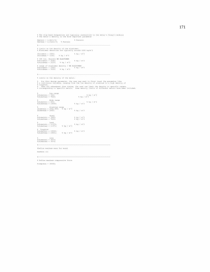
171
% The stop band frequencies are typically insensitive to the metal's Young's modulus% The metal's density is the more important parameter
Gmetmin = 2.0e11/3; % PascalsGmetmax = 2.01e11/3; % Pascals
%----------------------------------------------------------------------
% Limits on the density of the elastomer.% Elastomer densities are typically around 1000 kg/m^3
rhorubmin = 1000; % kg / m^3rhorubmax = 1100; % kg / m^3
% 30% vol. ferrite MR ELASTOMER%rhorubmin = 3330; % kg / m^3%rhorubmax = 3333; % kg / m^3
% range of elastomer density / MR ELASTOMER%rhorubmin = 1000; % kg / m^3%rhorubmax = 3333; % kg / m^3
%----------------------------------------------------------------------
% Limits on the density of the metal.
% For this design parameter, the user may want to first treat the parameter like% a continuous variable, ranging from the low density of aluminum to a high density of% tungsten.% Then for subsequent fine tuning, the user can limit the density to specific ranges,% corresponding to specific metals. Some density limits of different metals have been included.
% Low range%rhometmin = 700; % kg / m^3%rhometmax = 7820; % kg / m^3
% Wide range%rhometmin = 500; % kg / m^3%rhometmax = 19000; % kg / m^3
% Aluminum rangerhometmin = 2642.999; % kg / m^3rhometmax = 2643; % kg / m^3
% Steel%rhometmin = 7800; % kg / m^3%rhometmax = 7820; % kg / m^3
% Lead%rhometmin = 11370; % kg / m^3%rhometmax = 11371; % kg / m^3
% Tungsten%rhometmin = 19000; % kg / m^3%rhometmax = 19001; % kg / m^3
% iron%rhometmin = 7873;%rhometmax = 7874;
%----------------------------------------------------------------------
%Define maximum mass for mount
maxmass =2;
%----------------------------------------------------------------------
% Define maximum compressive force
Fcompress = 30000;
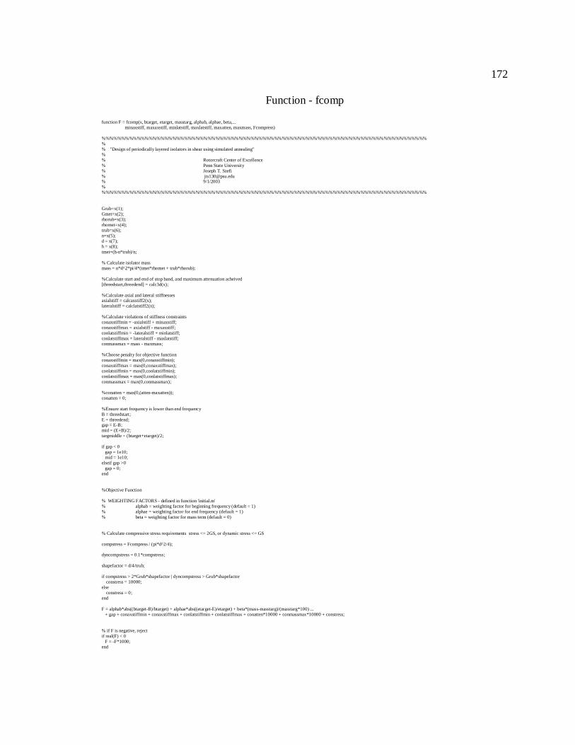
172
Function - fcomp
function F = fcomp(x, btarget, etarget, masstarg, alphab, alphae, beta,... minaxstiff, maxaxstiff, minlatstiff, maxlatstiff, maxatten, maxmass, Fcompress)
%%%%%%%%%%%%%%%%%%%%%%%%%%%%%%%%%%%%%%%%%%%%%%%%%%%%%%%%%%%%%%%%%%%%%%%%%%%%%%%%%%%%% "Design of periodically layered isolators in shear using simulated annealing"%% Rotorcraft Center of Excellence% Penn State University% Joseph T. Szefi% [email protected]% 9/1/2003%%%%%%%%%%%%%%%%%%%%%%%%%%%%%%%%%%%%%%%%%%%%%%%%%%%%%%%%%%%%%%%%%%%%%%%%%%%%%%%%%%%%
Grub=x(1);Gmet=x(2);rhorub=x(3);rhomet=x(4);trub=x(6);n=x(5);d = x(7);h = x(8);tmet=(h-n*trub)/n;
% Calculate isolator massmass = n*d^2*pi/4*(tmet*rhomet + trub*rhorub);
%Calculate start and end of stop band, and maximum attenuation acheived[threedstart,threedend] = calc3d(x);
%Calculate axial and lateral stiffnessesaxialstiff = calcaxstiff2(x);lateralstiff = calclatstiff2(x);
%Calculate violations of stiffness constraintsconaxstiffmin = -axialstiff + minaxstiff;conaxstiffmax = axialstiff - maxaxstiff;conlatstiffmin = -lateralstiff + minlatstiff;conlatstiffmax = lateralstiff - maxlatstiff;conmassmax = mass - maxmass;
%Choose penalty for objective functionconaxstiffmin = max(0,conaxstiffmin);conaxstiffmax = max(0,conaxstiffmax);conlatstiffmin = max(0,conlatstiffmin);conlatstiffmax = max(0,conlatstiffmax);conmassmax = max(0,conmassmax);
%conatten = max(0,(atten-maxatten));conatten = 0;
%Ensure start frequency is lower than end frequencyB = threedstart;E = threedend;gap = E-B;mid = (E+B)/2;targmiddle = (btarget+etarget)/2;
if gap < 0 gap = 1e10; mid = 1e10;elseif gap >0 gap = 0;end
%Objective Function
% WEIGHTING FACTORS - defined in function 'initial.m'% alphab = weighting factor for beginning frequency (default = 1)% alphae = weighting factor for end frequency (default = 1)% beta = weighting factor for mass term (default = 0)
% Calculate compressive stress requirements stress <= 2GS, or dynamic stress <= GS
compstress = Fcompress / (pi*d^2/4);
dyncompstress = 0.1*compstress;
shapefactor = d/4/trub;
if compstress > 2*Grub*shapefactor | dyncompstress > Grub*shapefactor constress = 10000;else constress = 0;end
F = alphab*abs((btarget-B)/btarget) + alphae*abs((etarget-E)/etarget) + beta*(mass-masstarg)/(masstarg*100) ... + gap + conaxstiffmin + conaxstiffmax + conlatstiffmin + conlatstiffmax + conatten*10000 + conmassmax*10000 + constress;
% if F is negative, rejectif real(F) < 0 F = -F*1000;end

173
Function – calc3D
function [threedstart,threedend] = calc3D(x)
%%%%%%%%%%%%%%%%%%%%%%%%%%%%%%%%%%%%%%%%%%%%%%%%%%%%%%%%%%%%%%%%%%%%%%%%%%%%%%%%%%%%% "Design of periodically layered isolators in compression using simulated annealing"%% Rotorcraft Center of Excellence% Penn State University% Joseph T. Szefi% [email protected]% 9/1/2003%%%%%%%%%%%%%%%%%%%%%%%%%%%%%%%%%%%%%%%%%%%%%%%%%%%%%%%%%%%%%%%%%%%%%%%%%%%%%%%%%%%%
Grub = x(1);Gmet = x(2);rhorub = x(3);rhomet = x(4);N = x(5);trub = x(6);d = x(7);height = x(8);tmetactual = (x(8)-N*trub)/N;
h = .00000000000001;
tmet = .00000000000001;n = 1;
h = h + trub;
metthick = tmet/h*2;Lz= h/2;Lr= d/2;
%Elastomer properties
rho1 = rhorub;nu1 = .499;G1 = Grub;
E1 = G1*2*(1+nu1);
Q1 = E1*(1-nu1)/(1+nu1)/(1-2*nu1);S1 = nu1/(1-nu1);
C111= Q1;C122= Q1;C133= Q1;C112= Q1*S1;C123= Q1*S1;C113= Q1*S1;C155= Q1*(1-2*nu1)/2/(1-nu1);
%Metal Properties%Metal layer is approximated with very thin layer with appropriate density
rho2 = rhomet;nu2 = .499;G2 = Gmet;
E2 = G2*2*(1+nu2);
Q2 = E2*(1-nu2)/(1+nu2)/(1-2*nu2);S2 = nu2/(1-nu2);
C211= Q2;C222= Q2;C233= Q2;C212= Q2*S2;C223= Q2*S2;C213= Q2*S2;C255= Q2*(1-2*nu2)/2/(1-nu2);
umax = 4;wmax = 8;
% Calculate components of global mass matrix
% The global matrices are in the following form
% |K11||K12|{a} - omega^2*|M11| |0|{a} = {0}% |K21||K22|{b} |0| |M22|{b} {0}%
clen = 2/n;
tbegin = -1;tend = -1 + clen;rho2 = rho2*tmetactual/tmet;
m = zeros((umax+wmax));k = zeros((umax+wmax));
%Loop through number of cells and calculate M and K matrices.for cell=1:n
% Calculation of M11 and M22 for elastomer and metalthickness = tend - metthick;
m(1,1)=2*pi*(1/30*(thickness)^5-1/30*tbegin^5-1/9*(thickness)^3+1/9*tbegin^3+1/6*tend-1/6*metthick-1/6*tbegin)*Lr^2*Lz*rho1... +2*pi*(1/30*tend^5-1/30*(thickness)^5-1/9*tend^3+1/9*(thickness)^3+1/6*metthick)*Lr^2*Lz*rho2;m(1,2)=2*pi*(1/25*(thickness)^5-1/25*tbegin^5-2/15*(thickness)^3+2/15*tbegin^3+1/5*tend-1/5*metthick-1/5*tbegin)*Lr^2*Lz*rho1... +2*pi*(1/25*tend^5-1/25*(thickness)^5-2/15*tend^3+2/15*(thickness)^3+1/5*metthick)*Lr^2*Lz*rho2;m(1,3)=2*pi*(1/36*(thickness)^6-1/36*tbegin^6-1/12*(thickness)^4+1/12*tbegin^4+1/12*(thickness)^2-1/12*tbegin^2)*Lr^2*Lz*rho1... +2*pi*(1/36*tend^6-1/36*(thickness)^6-1/12*tend^4+1/12*(thickness)^4+1/12*tend^2-1/12*(thickness)^2)*Lr^2*Lz*rho2;m(1,4)=2*pi*(1/30*(thickness)^6-1/30*tbegin^6-1/10*(thickness)^4+1/10*tbegin^4+1/10*(thickness)^2-1/10*tbegin^2)*Lr^2*Lz*rho1... +2*pi*(1/30*tend^6-1/30*(thickness)^6-1/10*tend^4+1/10*(thickness)^4+1/10*tend^2-1/10*(thickness)^2)*Lr^2*Lz*rho2;m(2,2)=2*pi*(1/20*(thickness)^5-1/20*tbegin^5-1/6*(thickness)^3+1/6*tbegin^3+1/4*tend-1/4*metthick-1/4*tbegin)*Lr^2*Lz*rho1... +2*pi*(1/20*tend^5-1/20*(thickness)^5-1/6*tend^3+1/6*(thickness)^3+1/4*metthick)*Lr^2*Lz*rho2;m(2,3)=2*pi*(1/30*(thickness)^6-1/30*tbegin^6-1/10*(thickness)^4+1/10*tbegin^4+1/10*(thickness)^2-1/10*tbegin^2)*Lr^2*Lz*rho1... +2*pi*(1/30*tend^6-1/30*(thickness)^6-1/10*tend^4+1/10*(thickness)^4+1/10*tend^2-1/10*(thickness)^2)*Lr^2*Lz*rho2;m(2,4)=2*pi*(1/24*(thickness)^6-1/24*tbegin^6-1/8*(thickness)^4+1/8*tbegin^4+1/8*(thickness)^2-1/8*tbegin^2)*Lr^2*Lz*rho1... +2*pi*(1/24*tend^6-1/24*(thickness)^6-1/8*tend^4+1/8*(thickness)^4+1/8*tend^2-1/8*(thickness)^2)*Lr^2*Lz*rho2;m(3,3)=2*pi*(1/42*(thickness)^7-1/42*tbegin^7-1/15*(thickness)^5+1/15*tbegin^5+1/18*(thickness)^3-1/18*tbegin^3)*Lr^2*Lz*rho1... +2*pi*(1/42*tend^7-1/42*(thickness)^7-1/15*tend^5+1/15*(thickness)^5+1/18*tend^3-1/18*(thickness)^3)*Lr^2*Lz*rho2;m(3,4)=2*pi*(1/35*(thickness)^7-1/35*tbegin^7-2/25*(thickness)^5+2/25*tbegin^5+1/15*(thickness)^3-1/15*tbegin^3)*Lr^2*Lz*rho1...

174
+2*pi*(1/35*tend^7-1/35*(thickness)^7-2/25*tend^5+2/25*(thickness)^5+1/15*tend^3-1/15*(thickness)^3)*Lr^2*Lz*rho2;m(4,4)=2*pi*(1/28*(thickness)^7-1/28*tbegin^7-1/10*(thickness)^5+1/10*tbegin^5+1/12*(thickness)^3-1/12*tbegin^3)*Lr^2*Lz*rho1... +2*pi*(1/28*tend^7-1/28*(thickness)^7-1/10*tend^5+1/10*(thickness)^5+1/12*tend^3-1/12*(thickness)^3)*Lr^2*Lz*rho2;m(5,5)=rho1*Lr^2*Lz*2*pi*(1/2*tend-1/2*metthick-1/2*tbegin) + rho2*Lr^2*Lz*pi*metthick;m(5,6)=rho1*Lr^2*Lz*2*pi*(1/4*(thickness)^2-1/4*tbegin^2+1/2*tend-1/2*metthick-1/2*tbegin)... + rho2*Lr^2*Lz*2*pi*(1/4*tend^2-1/4*(thickness)^2+1/2*metthick);m(5,7)=rho1*Lr^2*Lz*2*pi*(1/9*(thickness)^3-1/9*tbegin^3+1/6*tend-1/6*metthick-1/6*tbegin+1/4*(thickness)^2-1/4*tbegin^2)... + rho2*Lr^2*Lz*2*pi*(1/9*tend^3-1/9*(thickness)^3+1/6*metthick+1/4*tend^2-1/4*(thickness)^2);m(5,8)=rho1*Lr^2*Lz*2*pi*(1/6*(thickness)^3-1/6*tbegin^3+1/4*(thickness)^2-1/4*tbegin^2)... + rho2*Lr^2*Lz*2*pi*(1/6*tend^3-1/6*(thickness)^3+1/4*tend^2-1/4*(thickness)^2);m(5,9)=rho1*Lr^2*Lz*2*pi*(1/12*(thickness)^4-1/12*tbegin^4+1/12*(thickness)^2-1/12*tbegin^2+1/2*tend-1/2*metthick-1/2*tbegin)... + rho2*Lr^2*Lz*2*pi*(1/12*tend^4-1/12*(thickness)^4+1/12*tend^2-1/12*(thickness)^2+1/2*metthick);m(5,10)=rho1*Lr^2*Lz*2*pi*(1/8*(thickness)^4-1/8*tbegin^4+1/2*tend-1/2*metthick-1/2*tbegin)... + rho2*Lr^2*Lz*2*pi*(1/8*tend^4-1/8*(thickness)^4+1/2*metthick);m(5,11)=rho1*Lr^2*Lz*2*pi*(1/15*(thickness)^5-1/15*tbegin^5-1/9*(thickness)^3+1/9*tbegin^3+1/4*(thickness)^2-1/4*tbegin^2+... 1/2*tend-1/2*metthick-1/2*tbegin) + rho2*Lr^2*Lz*2*pi*(1/15*tend^5-1/15*(thickness)^5-1/9*tend^3+1/9*(thickness)^3+... 1/4*tend^2-1/4*(thickness)^2+1/2*metthick);m(5,12)=rho1*Lr^2*Lz*2*pi*(1/10*(thickness)^5-1/10*tbegin^5-1/6*(thickness)^3+1/6*tbegin^3+1/4*(thickness)^2-1/4*tbegin^2+... 1/2*tend-1/2*metthick-1/2*tbegin) + rho2*Lr^2*Lz*2*pi*(1/10*tend^5-1/10*(thickness)^5-1/6*tend^3+1/6*(thickness)^3+... 1/4*tend^2-1/4*(thickness)^2+1/2*metthick);m(6,6)=rho1*Lr^2*Lz*2*pi*(1/6*(thickness)^3-1/6*tbegin^3+1/2*(thickness)^2-1/2*tbegin^2+1/2*tend-1/2*metthick-1/2*tbegin)... + rho2*Lr^2*Lz*2*pi*(1/6*tend^3-1/6*(thickness)^3+1/2*tend^2-1/2*(thickness)^2+1/2*metthick);m(6,7)=rho1*Lr^2*Lz*2*pi*(1/12*(thickness)^4-1/12*tbegin^4+5/18*(thickness)^3-5/18*tbegin^3+1/3*(thickness)^2-1/3*tbegin^2+... 1/6*tend-1/6*metthick-1/6*tbegin) + rho2*Lr^2*Lz*2*pi*(1/12*tend^4-1/12*(thickness)^4+5/18*tend^3-5/18*(thickness)^3+... 1/3*tend^2-1/3*(thickness)^2+1/6*metthick);m(6,8)=rho1*Lr^2*Lz*2*pi*(1/8*(thickness)^4-1/8*tbegin^4+1/3*(thickness)^3-1/3*tbegin^3+1/4*(thickness)^2-1/4*tbegin^2)... + rho2*Lr^2*Lz*2*pi*(1/8*tend^4-1/8*(thickness)^4+1/3*tend^3-1/3*(thickness)^3+1/4*tend^2-1/4*(thickness)^2);m(6,9)=rho1*Lr^2*Lz*2*pi*(1/12*(thickness)^4-1/12*tbegin^4+1/18*(thickness)^3-1/18*tbegin^3+1/15*(thickness)^5-1/15*tbegin^5+... 1/3*(thickness)^2-1/3*tbegin^2+1/2*tend-1/2*metthick-1/2*tbegin) + rho2*Lr^2*Lz*2*pi*(1/12*tend^4-1/12*(thickness)^4+... 1/18*tend^3-1/18*(thickness)^3+1/15*tend^5-1/15*(thickness)^5+1/3*tend^2-1/3*(thickness)^2+1/2*metthick);m(6,10)=rho1*Lr^2*Lz*2*pi*(1/10*(thickness)^5-1/10*tbegin^5+1/8*(thickness)^4-1/8*tbegin^4+1/4*(thickness)^2-1/4*tbegin^2+... 1/2*tend-1/2*metthick-1/2*tbegin) + rho2*Lr^2*Lz*2*pi*(1/10*tend^5-1/10*(thickness)^5+1/8*tend^4-1/8*(thickness)^4+... 1/4*tend^2-1/4*(thickness)^2+1/2*metthick);m(6,11)=rho1*Lr^2*Lz*2*pi*(1/18*(thickness)^6-1/18*tbegin^6+1/18*(thickness)^3-1/18*tbegin^3+1/15*(thickness)^5-1/15*tbegin^5-... 1/12*(thickness)^4+1/12*tbegin^4+1/2*(thickness)^2-1/2*tbegin^2+1/2*tend-1/2*metthick-1/2*tbegin)... + rho2*Lr^2*Lz*2*pi*(1/18*tend^6-1/18*(thickness)^6+1/18*tend^3-1/18*(thickness)^3+1/15*tend^5-1/15*(thickness)^5-... 1/12*tend^4+1/12*(thickness)^4+1/2*tend^2-1/2*(thickness)^2+1/2*metthick);m(6,12)=rho1*Lr^2*Lz*2*pi*(1/12*(thickness)^6-1/12*tbegin^6+1/10*(thickness)^5-1/10*tbegin^5-1/8*(thickness)^4+1/8*tbegin^4+... 1/2*(thickness)^2-1/2*tbegin^2+1/2*tend-1/2*metthick-1/2*tbegin) + rho2*Lr^2*Lz*2*pi*(1/12*tend^6-1/12*(thickness)^6+... 1/10*tend^5-1/10*(thickness)^5-1/8*tend^4+1/8*(thickness)^4+1/2*tend^2-1/2*(thickness)^2+1/2*metthick);m(7,7)=rho1*Lr^2*Lz*2*pi*(1/20*(thickness)^5-1/20*tbegin^5+2/9*(thickness)^3-2/9*tbegin^3+1/12*tend-1/12*metthick-... 1/12*tbegin+1/6*(thickness)^4-1/6*tbegin^4+1/6*(thickness)^2-1/6*tbegin^2) + rho2*Lr^2*Lz*2*pi*(1/20*tend^5-... 1/20*(thickness)^5+2/9*tend^3-2/9*(thickness)^3+1/12*metthick+1/6*tend^4-1/6*(thickness)^4+1/6*tend^2-... 1/6*(thickness)^2);m(7,8)=rho1*Lr^2*Lz*2*pi*(5/24*(thickness)^4-5/24*tbegin^4+2/9*(thickness)^3-2/9*tbegin^3+1/15*(thickness)^5-... 1/15*tbegin^5+1/12*(thickness)^2-1/12*tbegin^2) + rho2*Lr^2*Lz*2*pi*(5/24*tend^4-5/24*(thickness)^4+2/9*tend^3-... 2/9*(thickness)^3+1/15*tend^5-1/15*(thickness)^5+1/12*tend^2-1/12*(thickness)^2);m(7,9)=rho1*Lr^2*Lz*2*pi*(1/24*(thickness)^4-1/24*tbegin^4+7/24*(thickness)^2-7/24*tbegin^2+1/24*(thickness)^6-... 1/24*tbegin^6+1/15*(thickness)^5-1/15*tbegin^5+1/6*tend-1/6*metthick-1/6*tbegin+1/6*(thickness)^3-1/6*tbegin^3)... + rho2*Lr^2*Lz*2*pi*(1/24*tend^4-1/24*(thickness)^4+7/24*tend^2-7/24*(thickness)^2+1/24*tend^6-1/24*... (thickness)^6+1/15*tend^5-1/15*(thickness)^5+1/6*metthick+1/6*tend^3-1/6*(thickness)^3);m(7,10)=rho1*Lr^2*Lz*2*pi*(1/18*(thickness)^6-1/18*tbegin^6+1/24*(thickness)^4-1/24*tbegin^4+1/9*(thickness)^3-1/9*tbegin^3+... 1/6*tend-1/6*metthick-1/6*tbegin+1/10*(thickness)^5-1/10*tbegin^5+1/4*(thickness)^2-1/4*tbegin^2) +... rho2*Lr^2*Lz*2*pi*(1/18*tend^6-1/18*(thickness)^6+1/24*tend^4-1/24*(thickness)^4+1/9*tend^3-1/9*(thickness)^3+... 1/6*metthick+1/10*tend^5-1/10*(thickness)^5+1/4*tend^2-1/4*(thickness)^2);m(7,11)=rho1*Lr^2*Lz*2*pi*(-1/30*(thickness)^5+1/30*tbegin^5+1/28*(thickness)^7-1/28*tbegin^7+1/4*(thickness)^3-... 1/4*tbegin^3+1/18*(thickness)^6-1/18*tbegin^6+1/3*(thickness)^2-1/3*tbegin^2+1/6*tend-1/6*metthick-1/6*tbegin)... + rho2*Lr^2*Lz*2*pi*(-1/30*tend^5+1/30*(thickness)^5+1/28*tend^7-1/28*(thickness)^7+1/4*tend^3-1/4*(thickness)^3+... 1/18*tend^6-1/18*(thickness)^6+1/3*tend^2-1/3*(thickness)^2+1/6*metthick);m(7,12)=rho1*Lr^2*Lz*2*pi*(1/21*(thickness)^7-1/21*tbegin^7+2/9*(thickness)^3-2/9*tbegin^3-1/30*(thickness)^5+... 1/30*tbegin^5+1/3*(thickness)^2-1/3*tbegin^2-1/24*(thickness)^4+1/24*tbegin^4+1/6*tend-1/6*metthick-1/6*tbegin+... 1/12*(thickness)^6-1/12*tbegin^6) + rho2*Lr^2*Lz*2*pi*(1/21*tend^7-1/21*(thickness)^7+2/9*tend^3-2/9*(thickness)^3-... 1/30*tend^5+1/30*(thickness)^5+1/3*tend^2-1/3*(thickness)^2-1/24*tend^4+1/24*(thickness)^4+1/6*metthick+1/12*tend^6-... 1/12*(thickness)^6);m(8,8)=rho1*Lr^2*Lz*2*pi*(1/10*(thickness)^5-1/10*tbegin^5+1/4*(thickness)^4-1/4*tbegin^4+1/6*(thickness)^3-1/6*tbegin^3)... + rho2*Lr^2*Lz*2*pi*(1/10*tend^5-1/10*(thickness)^5+1/4*tend^4-1/4*(thickness)^4+1/6*tend^3-1/6*(thickness)^3);m(8,9)=rho1*Lr^2*Lz*2*pi*(1/18*(thickness)^6-1/18*tbegin^6+2/9*(thickness)^3-2/9*tbegin^3+1/15*(thickness)^5-1/15*tbegin^5+... 1/24*(thickness)^4-1/24*tbegin^4+1/4*(thickness)^2-1/4*tbegin^2) + rho2*Lr^2*Lz*2*pi*(1/18*tend^6-1/18*(thickness)^6+... 2/9*tend^3-2/9*(thickness)^3+1/15*tend^5-1/15*(thickness)^5+1/24*tend^4-1/24*(thickness)^4+1/4*tend^2-1/4*(thickness)^2);m(8,10)=rho1*Lr^2*Lz*2*pi*(1/12*(thickness)^6-1/12*tbegin^6+1/10*(thickness)^5-1/10*tbegin^5+1/6*(thickness)^3-1/6*tbegin^3+... 1/4*(thickness)^2-1/4*tbegin^2) + rho2*Lr^2*Lz*2*pi*(1/12*tend^6-1/12*(thickness)^6+1/10*tend^5-1/10*(thickness)^5+... 1/6*tend^3-1/6*(thickness)^3+1/4*tend^2-1/4*(thickness)^2);m(8,11)=rho1*Lr^2*Lz*2*pi*(1/21*(thickness)^7-1/21*tbegin^7+1/24*(thickness)^4-1/24*tbegin^4+1/18*(thickness)^6-... 1/18*tbegin^6-1/15*(thickness)^5+1/15*tbegin^5+1/3*(thickness)^3-1/3*tbegin^3+1/4*(thickness)^2-1/4*tbegin^2)... + rho2*Lr^2*Lz*2*pi*(1/21*tend^7-1/21*(thickness)^7+1/24*tend^4-1/24*(thickness)^4+1/18*tend^6-1/18*... (thickness)^6-1/15*tend^5+1/15*(thickness)^5+1/3*tend^3-1/3*(thickness)^3+1/4*tend^2-1/4*(thickness)^2);m(8,12)=rho1*Lr^2*Lz*2*pi*(1/14*(thickness)^7-1/14*tbegin^7+1/12*(thickness)^6-1/12*tbegin^6-1/10*(thickness)^5+... 1/10*tbegin^5+1/3*(thickness)^3-1/3*tbegin^3+1/4*(thickness)^2-1/4*tbegin^2) + rho2*Lr^2*Lz*2*pi*(1/14*tend^7-... 1/14*(thickness)^7+1/12*tend^6-1/12*(thickness)^6-1/10*tend^5+1/10*(thickness)^5+1/3*tend^3-1/3*(thickness)^3+... 1/4*tend^2-1/4*(thickness)^2);m(9,9)=rho1*Lr^2*Lz*2*pi*(1/30*(thickness)^5-1/30*tbegin^5+1/28*(thickness)^7-1/28*tbegin^7+1/36*(thickness)^3-... 1/36*tbegin^3+1/6*(thickness)^2-1/6*tbegin^2+1/6*(thickness)^4-1/6*tbegin^4+1/2*tend-1/2*metthick-1/2*tbegin)... + rho2*Lr^2*Lz*2*pi*(1/30*tend^5-1/30*(thickness)^5+1/28*tend^7-1/28*(thickness)^7+1/36*tend^3-1/36*(thickness)^3+... 1/6*tend^2-1/6*(thickness)^2+1/6*tend^4-1/6*(thickness)^4+1/2*metthick);m(9,10)=rho1*Lr^2*Lz*2*pi*(1/21*(thickness)^7-1/21*tbegin^7+1/30*(thickness)^5-1/30*tbegin^5+5/24*(thickness)^4-5/24*tbegin^4+... 1/12*(thickness)^2-1/12*tbegin^2+1/2*tend-1/2*metthick-1/2*tbegin) + rho2*Lr^2*Lz*2*pi*(1/21*tend^7-1/21*(thickness)^7+... 1/30*tend^5-1/30*(thickness)^5+5/24*tend^4-5/24*(thickness)^4+1/12*tend^2-1/12*(thickness)^2+1/2*metthick);m(9,11)=rho1*Lr^2*Lz*2*pi*(1/32*(thickness)^8-1/32*tbegin^8-1/36*(thickness)^6+1/36*tbegin^6+1/16*(thickness)^4-... 1/16*tbegin^4+1/3*(thickness)^2-1/3*tbegin^2-1/18*(thickness)^3+1/18*tbegin^3+2/15*(thickness)^5-2/15*tbegin^5+... 1/2*tend-1/2*metthick-1/2*tbegin) + rho2*Lr^2*Lz*2*pi*(1/32*tend^8-1/32*(thickness)^8-1/36*tend^6+1/36*(thickness)^6+... 1/16*tend^4-1/16*(thickness)^4+1/3*tend^2-1/3*(thickness)^2-1/18*tend^3+1/18*(thickness)^3+2/15*tend^5-... 2/15*(thickness)^5+1/2*metthick);m(9,12)=rho1*Lr^2*Lz*2*pi*(1/24*(thickness)^8-1/24*tbegin^8-1/36*(thickness)^6+1/36*tbegin^6-1/9*(thickness)^3+... 1/9*tbegin^3+1/6*(thickness)^5-1/6*tbegin^5+1/3*(thickness)^2-1/3*tbegin^2+1/24*(thickness)^4-1/24*tbegin^4+... 1/2*tend-1/2*metthick-1/2*tbegin) + rho2*Lr^2*Lz*2*pi*(1/24*tend^8-1/24*(thickness)^8-1/36*tend^6+1/36*(thickness)^6-... 1/9*tend^3+1/9*(thickness)^3+1/6*tend^5-1/6*(thickness)^5+1/3*tend^2-1/3*(thickness)^2+1/24*tend^4-1/24*(thickness)^4+... 1/2*metthick);m(10,10)=rho1*Lr^2*Lz*2*pi*(1/14*(thickness)^7-1/14*tbegin^7+1/4*(thickness)^4-1/4*tbegin^4+1/2*tend-1/2*metthick-1/2*tbegin)... + rho2*Lr^2*Lz*2*pi*(1/14*tend^7-1/14*(thickness)^7+1/4*tend^4-1/4*(thickness)^4+1/2*metthick);m(10,11)=rho1*Lr^2*Lz*2*pi*(-1/18*(thickness)^6+1/18*tbegin^6+1/24*(thickness)^8-1/24*tbegin^8-1/9*(thickness)^3+... 1/9*tbegin^3+1/6*(thickness)^5-1/6*tbegin^5+1/8*(thickness)^4-1/8*tbegin^4+1/4*(thickness)^2-1/4*tbegin^2+... 1/2*tend-1/2*metthick-1/2*tbegin) + rho2*Lr^2*Lz*2*pi*(-1/18*tend^6+1/18*(thickness)^6+1/24*tend^8-... 1/24*(thickness)^8-1/9*tend^3+1/9*(thickness)^3+1/6*tend^5-1/6*(thickness)^5+1/8*tend^4-1/8*(thickness)^4+... 1/4*tend^2-1/4*(thickness)^2+1/2*metthick);m(10,12)=rho1*Lr^2*Lz*2*pi*(1/16*(thickness)^8-1/16*tbegin^8-1/12*(thickness)^6+1/12*tbegin^6+1/5*(thickness)^5-... 1/5*tbegin^5+1/8*(thickness)^4-1/8*tbegin^4-1/6*(thickness)^3+1/6*tbegin^3+1/4*(thickness)^2-1/4*tbegin^2+1/2*tend... -1/2*metthick-1/2*tbegin) + rho2*Lr^2*Lz*2*pi*(1/16*tend^8-1/16*(thickness)^8-1/12*tend^6+1/12*(thickness)^6+... 1/5*tend^5-1/5*(thickness)^5+1/8*tend^4-1/8*(thickness)^4-1/6*tend^3+1/6*(thickness)^3+1/4*tend^2-1/4*(thickness)^2+... 1/2*metthick);m(11,11)=rho1*Lr^2*Lz*2*pi*(1/36*(thickness)^9-1/36*tbegin^9+11/60*(thickness)^5-11/60*tbegin^5-1/14*(thickness)^7+... 1/14*tbegin^7-1/6*(thickness)^4+1/6*tbegin^4+1/9*(thickness)^6-1/9*tbegin^6-1/18*(thickness)^3+1/18*tbegin^3+... 1/2*(thickness)^2-1/2*tbegin^2+1/2*tend-1/2*metthick-1/2*tbegin) + rho2*Lr^2*Lz*2*pi*(1/36*tend^9-1/36*(thickness)^9+... 11/60*tend^5-11/60*(thickness)^5-1/14*tend^7+1/14*(thickness)^7-1/6*tend^4+1/6*(thickness)^4+1/9*tend^6-1/9*(thickness)^6-... 1/18*tend^3+1/18*(thickness)^3+1/2*tend^2-1/2*(thickness)^2+1/2*metthick);m(11,12)=rho1*Lr^2*Lz*2*pi*(5/36*(thickness)^6-5/36*tbegin^6+1/27*(thickness)^9-1/27*tbegin^9-2/21*(thickness)^7+... 2/21*tbegin^7-5/24*(thickness)^4+5/24*tbegin^4-1/9*(thickness)^3+1/9*tbegin^3+7/30*(thickness)^5-7/30*tbegin^5+... 1/2*(thickness)^2-1/2*tbegin^2+1/2*tend-1/2*metthick-1/2*tbegin) + rho2*Lr^2*Lz*2*pi*(5/36*tend^6-5/36*(thickness)^6+... 1/27*tend^9-1/27*(thickness)^9-2/21*tend^7+2/21*(thickness)^7-5/24*tend^4+5/24*(thickness)^4-1/9*tend^3+1/9*(thickness)^3+... 7/30*tend^5-7/30*(thickness)^5+1/2*tend^2-1/2*(thickness)^2+1/2*metthick);m(12,12)=rho1*Lr^2*Lz*2*pi*(1/18*(thickness)^9-1/18*tbegin^9-1/7*(thickness)^7+1/7*tbegin^7+1/6*(thickness)^6-1/6*tbegin^6+... 3/10*(thickness)^5-3/10*tbegin^5-1/4*(thickness)^4+1/4*tbegin^4-1/6*(thickness)^3+1/6*tbegin^3+1/2*(thickness)^2-... 1/2*tbegin^2+1/2*tend-1/2*metthick-1/2*tbegin) + rho2*Lr^2*Lz*2*pi*(1/18*tend^9-1/18*(thickness)^9-1/7*tend^7+... 1/7*(thickness)^7+1/6*tend^6-1/6*(thickness)^6+3/10*tend^5-3/10*(thickness)^5-1/4*tend^4+1/4*(thickness)^4-... 1/6*tend^3+1/6*(thickness)^3+1/2*tend^2-1/2*(thickness)^2+1/2*metthick);

175
temp = triu(m(1:umax,1:umax),1);temp = m(1:umax,1:umax) + temp';m(1:umax, 1:umax) = temp;temp = triu(m((umax+1):(umax+wmax),(umax+1):(umax+wmax)),1);temp = m((umax+1):(umax+wmax),(umax+1):(umax+wmax)) + temp';m((umax+1):(umax+wmax),(umax+1):(umax+wmax)) = temp;
%Calculation of K11 for elastomer and metal
k(1,1)=2*pi*(1/20*(4*C111/Lr^2+C122/Lr^2+4*C112/Lr^2)*Lr^2*Lz*((thickness)^5-tbegin^5)+1/3*(2/3*C155/Lz*Lr^2+... 1/4*(-8*C111/Lr^2-8*C112/Lr^2-2*C122/Lr^2)*Lr^2*Lz)*((thickness)^3-tbegin^3)+1/4*(4*C111/Lr^2+C122/Lr^2+... 4*C112/Lr^2)*Lr^2*Lz*(tend-metthick-tbegin))+2*pi*(1/20*(4*C211/Lr^2+C222/Lr^2+4*C212/Lr^2)*Lr^2*Lz*(tend^5-... (thickness)^5)+1/3*(2/3*C255/Lz*Lr^2+1/4*(-8*C211/Lr^2-8*C212/Lr^2-2*C222/Lr^2)*Lr^2*Lz)*(tend^3-(thickness)^3)+... 1/4*(4*C211/Lr^2+C222/Lr^2+4*C212/Lr^2)*Lr^2*Lz*metthick);k(1,2)=2*pi*(1/15*(2*C111/Lr^2+C122/Lr^2+3*C112/Lr^2)*Lr^2*Lz*((thickness)^5-tbegin^5)+1/3*(4/5*C155/Lz*Lr^2+... 1/3*(-4*C111/Lr^2-6*C112/Lr^2-2*C122/Lr^2)*Lr^2*Lz)*((thickness)^3-tbegin^3)+1/3*(2*C111/Lr^2+C122/Lr^2+... 3*C112/Lr^2)*Lr^2*Lz*(tend-metthick-tbegin))+2*pi*(1/15*(2*C211/Lr^2+C222/Lr^2+3*C212/Lr^2)*Lr^2*Lz*(tend^5-... (thickness)^5)+1/3*(4/5*C255/Lz*Lr^2+1/3*(-4*C211/Lr^2-6*C212/Lr^2-2*C222/Lr^2)*Lr^2*Lz)*(tend^3-(thickness)^3)+... 1/3*(2*C211/Lr^2+C222/Lr^2+3*C212/Lr^2)*Lr^2*Lz*metthick);k(1,3)=2*pi*(1/24*(4*C111/Lr^2+C122/Lr^2+4*C112/Lr^2)*Lr^2*Lz*((thickness)^6-tbegin^6)+1/4*(C155/Lz*Lr^2+... 1/4*(-8*C111/Lr^2-8*C112/Lr^2-2*C122/Lr^2)*Lr^2*Lz)*((thickness)^4-tbegin^4)+1/2*(-1/3*C155/Lz*Lr^2+... 1/4*(4*C111/Lr^2+C122/Lr^2+4*C112/Lr^2)*Lr^2*Lz)*((thickness)^2-tbegin^2))+2*pi*(1/24*(4*C211/Lr^2+C222/Lr^2+... 4*C212/Lr^2)*Lr^2*Lz*(tend^6-(thickness)^6)+1/4*(C255/Lz*Lr^2+1/4*(-8*C211/Lr^2-8*C212/Lr^2-... 2*C222/Lr^2)*Lr^2*Lz)*(tend^4-(thickness)^4)+1/2*(-1/3*C255/Lz*Lr^2+1/4*(4*C211/Lr^2+C222/Lr^2+... 4*C212/Lr^2)*Lr^2*Lz)*(tend^2-(thickness)^2));k(1,4)=2*pi*(1/18*(2*C111/Lr^2+C122/Lr^2+3*C112/Lr^2)*Lr^2*Lz*((thickness)^6-tbegin^6)+1/4*(6/5*C155/Lz*Lr^2+... 1/3*(-4*C111/Lr^2-6*C112/Lr^2-2*C122/Lr^2)*Lr^2*Lz)*((thickness)^4-tbegin^4)+1/2*(-2/5*C155/Lz*Lr^2+... 1/3*(2*C111/Lr^2+C122/Lr^2+3*C112/Lr^2)*Lr^2*Lz)*((thickness)^2-tbegin^2))+2*pi*(1/18*(2*C211/Lr^2+... C222/Lr^2+3*C212/Lr^2)*Lr^2*Lz*(tend^6-(thickness)^6)+1/4*(6/5*C255/Lz*Lr^2+1/3*(-4*C211/Lr^2-... 6*C212/Lr^2-2*C222/Lr^2)*Lr^2*Lz)*(tend^4-(thickness)^4)+1/2*(-2/5*C255/Lz*Lr^2+1/3*(2*C211/Lr^2+... C222/Lr^2+3*C212/Lr^2)*Lr^2*Lz)*(tend^2-(thickness)^2));k(2,2)=2*pi*(1/10*(C111/Lr^2+C122/Lr^2+2*C112/Lr^2)*Lr^2*Lz*((thickness)^5-tbegin^5)+1/3*(C155/Lz*Lr^2+... 1/2*(-2*C111/Lr^2-4*C112/Lr^2-2*C122/Lr^2)*Lr^2*Lz)*((thickness)^3-tbegin^3)+1/2*(C111/Lr^2+C122/Lr^2+... 2*C112/Lr^2)*Lr^2*Lz*(tend-metthick-tbegin))+2*pi*(1/10*(C211/Lr^2+C222/Lr^2+2*C212/Lr^2)*Lr^2*Lz*(tend^5-... (thickness)^5)+1/3*(C255/Lz*Lr^2+1/2*(-2*C211/Lr^2-4*C212/Lr^2-2*C222/Lr^2)*Lr^2*Lz)*(tend^3-(thickness)^3)+... 1/2*(C211/Lr^2+C222/Lr^2+2*C212/Lr^2)*Lr^2*Lz*metthick);k(2,3)=2*pi*(1/18*(2*C111/Lr^2+C122/Lr^2+3*C112/Lr^2)*Lr^2*Lz*((thickness)^6-tbegin^6)+1/4*(6/5*C155/Lz*Lr^2+... 1/3*(-4*C111/Lr^2-6*C112/Lr^2-2*C122/Lr^2)*Lr^2*Lz)*((thickness)^4-tbegin^4)+1/2*(-2/5*C155/Lz*Lr^2+... 1/3*(2*C111/Lr^2+C122/Lr^2+3*C112/Lr^2)*Lr^2*Lz)*((thickness)^2-tbegin^2))+2*pi*(1/18*(2*C211/Lr^2+... C222/Lr^2+3*C212/Lr^2)*Lr^2*Lz*(tend^6-(thickness)^6)+1/4*(6/5*C255/Lz*Lr^2+1/3*(-4*C211/Lr^2-6*C212/Lr^2-... 2*C222/Lr^2)*Lr^2*Lz)*(tend^4-(thickness)^4)+1/2*(-2/5*C255/Lz*Lr^2+1/3*(2*C211/Lr^2+C222/Lr^2+... 3*C212/Lr^2)*Lr^2*Lz)*(tend^2-(thickness)^2));k(2,4)=2*pi*(1/12*(C111/Lr^2+C122/Lr^2+2*C112/Lr^2)*Lr^2*Lz*((thickness)^6-tbegin^6)+1/4*(3/2*C155/Lz*Lr^2+... 1/2*(-2*C111/Lr^2-4*C112/Lr^2-2*C122/Lr^2)*Lr^2*Lz)*((thickness)^4-tbegin^4)+1/2*(-1/2*C155/Lz*Lr^2+... 1/2*(C111/Lr^2+C122/Lr^2+2*C112/Lr^2)*Lr^2*Lz)*((thickness)^2-tbegin^2))+2*pi*(1/12*(C211/Lr^2+C222/Lr^2+... 2*C212/Lr^2)*Lr^2*Lz*(tend^6-(thickness)^6)+1/4*(3/2*C255/Lz*Lr^2+1/2*(-2*C211/Lr^2-4*C212/Lr^2-... 2*C222/Lr^2)*Lr^2*Lz)*(tend^4-(thickness)^4)+1/2*(-1/2*C255/Lz*Lr^2+1/2*(C211/Lr^2+C222/Lr^2+... 2*C212/Lr^2)*Lr^2*Lz)*(tend^2-(thickness)^2));k(3,3)=2*pi*(1/28*(4*C111/Lr^2+C122/Lr^2+4*C112/Lr^2)*Lr^2*Lz*((thickness)^7-tbegin^7)+1/5*(3/2*C155/Lz*Lr^2+... 1/4*(-8*C111/Lr^2-8*C112/Lr^2-2*C122/Lr^2)*Lr^2*Lz)*((thickness)^5-tbegin^5)+1/3*(-C155/Lz*Lr^2+... 1/4*(4*C111/Lr^2+C122/Lr^2+4*C112/Lr^2)*Lr^2*Lz)*((thickness)^3-tbegin^3)+1/6*C155/Lz*Lr^2*(tend-metthick-tbegin))+... 2*pi*(1/28*(4*C211/Lr^2+C222/Lr^2+4*C212/Lr^2)*Lr^2*Lz*(tend^7-(thickness)^7)+1/5*(3/2*C255/Lz*Lr^2+... 1/4*(-8*C211/Lr^2-8*C212/Lr^2-2*C222/Lr^2)*Lr^2*Lz)*(tend^5-(thickness)^5)+... 1/3*(-C255/Lz*Lr^2+1/4*(4*C211/Lr^2+C222/Lr^2+4*C212/Lr^2)*Lr^2*Lz)*(tend^3-(thickness)^3)+1/6*C255/Lz*Lr^2*metthick);k(3,4)=2*pi*(1/21*(2*C111/Lr^2+C122/Lr^2+3*C112/Lr^2)*Lr^2*Lz*((thickness)^7-tbegin^7)+1/5*(9/5*C155/Lz*Lr^2+... 1/3*(-4*C111/Lr^2-6*C112/Lr^2-2*C122/Lr^2)*Lr^2*Lz)*((thickness)^5-tbegin^5)+1/3*(-6/5*C155/Lz*Lr^2+... 1/3*(2*C111/Lr^2+C122/Lr^2+3*C112/Lr^2)*Lr^2*Lz)*((thickness)^3-tbegin^3)+1/5*C155/Lz*Lr^2*(tend-metthick-tbegin))+... 2*pi*(1/21*(2*C211/Lr^2+C222/Lr^2+3*C212/Lr^2)*Lr^2*Lz*(tend^7-(thickness)^7)+1/5*(9/5*C255/Lz*Lr^2+... 1/3*(-4*C211/Lr^2-6*C212/Lr^2-2*C222/Lr^2)*Lr^2*Lz)*(tend^5-(thickness)^5)+1/3*(-6/5*C255/Lz*Lr^2+... 1/3*(2*C211/Lr^2+C222/Lr^2+3*C212/Lr^2)*Lr^2*Lz)*(tend^3-(thickness)^3)+1/5*C255/Lz*Lr^2*metthick);k(4,4)=2*pi*(1/14*(C111/Lr^2+C122/Lr^2+2*C112/Lr^2)*Lr^2*Lz*((thickness)^7-tbegin^7)+1/5*(9/4*C155/Lz*Lr^2+... 1/2*(-2*C111/Lr^2-4*C112/Lr^2-2*C122/Lr^2)*Lr^2*Lz)*((thickness)^5-tbegin^5)+1/3*(-3/2*C155/Lz*Lr^2+1/2*(C111/Lr^2+... C122/Lr^2+2*C112/Lr^2)*Lr^2*Lz)*((thickness)^3-tbegin^3)+1/4*C155/Lz*Lr^2*(tend-metthick-tbegin))+... 2*pi*(1/14*(C211/Lr^2+C222/Lr^2+2*C212/Lr^2)*Lr^2*Lz*(tend^7-(thickness)^7)+1/5*(9/4*C255/Lz*Lr^2+... 1/2*(-2*C211/Lr^2-4*C212/Lr^2-2*C222/Lr^2)*Lr^2*Lz)*(tend^5-(thickness)^5)+1/3*(-3/2*C255/Lz*Lr^2+1/2*(C211/Lr^2+... C222/Lr^2+2*C212/Lr^2)*Lr^2*Lz)*(tend^3-(thickness)^3)+1/4*C255/Lz*Lr^2*metthick);
temp = triu(k(1:umax,1:umax),1);temp = k(1:umax,1:umax) + temp';k(1:umax, 1:umax) = temp;
%Calculation of K12 for elastomer and metal
k(1,5)=0;k(1,6)=2*pi*(1/9*(2*C113/Lr/Lz+C123/Lr/Lz)*Lr^2*Lz*((thickness)^3-tbegin^3)+1/3*(-2*C113/Lr/Lz-C123/Lr/Lz)*Lr^2*Lz*(tend-... metthick-tbegin))+2*pi*(1/9*(2*C213/Lr/Lz+C223/Lr/Lz)*Lr^2*Lz*(tend^3-(thickness)^3)+1/3*(-2*C213/Lr/Lz-... C223/Lr/Lz)*Lr^2*Lz*metthick);k(1,7)=2*pi*(1/16*(4*C113/Lr/Lz+2*C123/Lr/Lz+2*C155/Lr/Lz)*Lr^2*Lz*((thickness)^4-tbegin^4)+... 1/9*(2*C113/Lr/Lz+C123/Lr/Lz)*Lr^2*Lz*((thickness)^3-tbegin^3)+1/8*(-4*C113/Lr/Lz-2*C123/Lr/Lz-... 2*C155/Lr/Lz)*Lr^2*Lz*((thickness)^2-tbegin^2)+1/3*(-2*C113/Lr/Lz-C123/Lr/Lz)*Lr^2*Lz*(tend-metthick-tbegin))+... 2*pi*(1/16*(4*C213/Lr/Lz+2*C223/Lr/Lz+2*C255/Lr/Lz)*Lr^2*Lz*(tend^4-(thickness)^4)+... 1/9*(2*C213/Lr/Lz+C223/Lr/Lz)*Lr^2*Lz*(tend^3-(thickness)^3)+1/8*(-4*C213/Lr/Lz-2*C223/Lr/Lz-... 2*C255/Lr/Lz)*Lr^2*Lz*(tend^2-(thickness)^2)+1/3*(-2*C213/Lr/Lz-C223/Lr/Lz)*Lr^2*Lz*metthick);k(1,8)=2*pi*(1/12*(4*C113/Lr/Lz+2*C123/Lr/Lz)*Lr^2*Lz*((thickness)^4-tbegin^4)+1/9*(2*C113/Lr/Lz+... C123/Lr/Lz)*Lr^2*Lz*((thickness)^3-tbegin^3)+1/6*(-4*C113/Lr/Lz-2*C123/Lr/Lz)*Lr^2*Lz*((thickness)^2-... tbegin^2)+1/3*(-2*C113/Lr/Lz-C123/Lr/Lz)*Lr^2*Lz*(tend-metthick-tbegin))+2*pi*(1/12*(4*C213/Lr/Lz+... 2*C223/Lr/Lz)*Lr^2*Lz*(tend^4-(thickness)^4)+1/9*(2*C213/Lr/Lz+C223/Lr/Lz)*Lr^2*Lz*(tend^3-(thickness)^3)+... 1/6*(-4*C213/Lr/Lz-2*C223/Lr/Lz)*Lr^2*Lz*(tend^2-(thickness)^2)+1/3*(-2*C213/Lr/Lz-C223/Lr/Lz)*Lr^2*Lz*metthick);k(1,9)=2*pi*(1/20*(3*C123/Lr/Lz+6*C113/Lr/Lz+2*C155/Lr/Lz)*Lr^2*Lz*((thickness)^5-tbegin^5)+... 1/3*(1/4*(-8*C113/Lr/Lz-2*C155/Lr/Lz-4*C123/Lr/Lz)*Lr^2*Lz+1/3*(2*C113/Lr/Lz+C123/Lr/Lz)*Lr^2*Lz)*((thickness)^3-... tbegin^3)+1/4*(2*C113/Lr/Lz+C123/Lr/Lz)*Lr^2*Lz*(tend-metthick-tbegin)+1/3*(-2*C113/Lr/Lz-... C123/Lr/Lz)*Lr^2*Lz*(tend-metthick-tbegin))+2*pi*(1/20*(3*C223/Lr/Lz+6*C213/Lr/Lz+2*C255/Lr/Lz)*Lr^2*Lz*(tend^5-... (thickness)^5)+1/3*(1/4*(-8*C213/Lr/Lz-2*C255/Lr/Lz-4*C223/Lr/Lz)*Lr^2*Lz+1/3*(2*C213/Lr/Lz+... C223/Lr/Lz)*Lr^2*Lz)*(tend^3-(thickness)^3)+1/4*(2*C213/Lr/Lz+C223/Lr/Lz)*Lr^2*Lz*metthick+... 1/3*(-2*C213/Lr/Lz-C223/Lr/Lz)*Lr^2*Lz*metthick);k(1,10)=2*pi*(1/15*(6*C113/Lr/Lz+3*C123/Lr/Lz)*Lr^2*Lz*((thickness)^5-tbegin^5)+1/9*(-6*C113/Lr/Lz-... 3*C123/Lr/Lz)*Lr^2*Lz*((thickness)^3-tbegin^3))+2*pi*(1/15*(6*C213/Lr/Lz+3*C223/Lr/Lz)*Lr^2*Lz*(tend^5-... (thickness)^5)+1/9*(-6*C213/Lr/Lz-3*C223/Lr/Lz)*Lr^2*Lz*(tend^3-(thickness)^3));k(1,11)=2*pi*(1/24*(4*C123/Lr/Lz+8*C113/Lr/Lz+2*C155/Lr/Lz)*Lr^2*Lz*((thickness)^6-tbegin^6)+... 1/16*(-12*C113/Lr/Lz-2*C155/Lr/Lz-6*C123/Lr/Lz)*Lr^2*Lz*((thickness)^4-tbegin^4)+... 1/9*(2*C113/Lr/Lz+C123/Lr/Lz)*Lr^2*Lz*((thickness)^3-tbegin^3)+1/8*(4*C113/Lr/Lz+2*C123/Lr/Lz)*Lr^2*Lz*((thickness)^2-... tbegin^2)+1/3*(-2*C113/Lr/Lz-C123/Lr/Lz)*Lr^2*Lz*(tend-metthick-tbegin))+2*pi*(1/24*(4*C223/Lr/Lz+8*C213/Lr/Lz+... 2*C255/Lr/Lz)*Lr^2*Lz*(tend^6-(thickness)^6)+1/16*(-12*C213/Lr/Lz-2*C255/Lr/Lz-6*C223/Lr/Lz)*Lr^2*Lz*(tend^4-... (thickness)^4)+1/9*(2*C213/Lr/Lz+C223/Lr/Lz)*Lr^2*Lz*(tend^3-(thickness)^3)+1/8*(4*C213/Lr/Lz+2*C223/Lr/Lz)*Lr^2*Lz*(tend^2-... (thickness)^2)+1/3*(-2*C213/Lr/Lz-C223/Lr/Lz)*Lr^2*Lz*metthick);k(1,12)=2*pi*(1/18*(8*C113/Lr/Lz+4*C123/Lr/Lz)*Lr^2*Lz*((thickness)^6-tbegin^6)+1/12*(-6*C123/Lr/Lz-... 12*C113/Lr/Lz)*Lr^2*Lz*((thickness)^4-tbegin^4)+1/9*(2*C113/Lr/Lz+C123/Lr/Lz)*Lr^2*Lz*((thickness)^3-... tbegin^3)+1/6*(4*C113/Lr/Lz+2*C123/Lr/Lz)*Lr^2*Lz*((thickness)^2-tbegin^2)+1/3*(-2*C113/Lr/Lz-... C123/Lr/Lz)*Lr^2*Lz*(tend-metthick-tbegin))+2*pi*(1/18*(8*C213/Lr/Lz+4*C223/Lr/Lz)*Lr^2*Lz*(tend^6-... (thickness)^6)+1/12*(-6*C223/Lr/Lz-12*C213/Lr/Lz)*Lr^2*Lz*(tend^4-(thickness)^4)+... 1/9*(2*C213/Lr/Lz+C223/Lr/Lz)*Lr^2*Lz*(tend^3-(thickness)^3)+1/6*(4*C213/Lr/Lz+2*C223/Lr/Lz)*Lr^2*Lz*(tend^2-... (thickness)^2)+1/3*(-2*C213/Lr/Lz-C223/Lr/Lz)*Lr^2*Lz*metthick);k(2,5)=0;k(2,6)=2*pi*(1/6*(C113/Lr/Lz+C123/Lr/Lz)*Lr^2*Lz*((thickness)^3-tbegin^3)+1/2*(-C113/Lr/Lz-C123/Lr/Lz)*Lr^2*Lz*(tend-... metthick-tbegin))+2*pi*(1/6*(C213/Lr/Lz+C223/Lr/Lz)*Lr^2*Lz*(tend^3-(thickness)^3)+1/2*(-C213/Lr/Lz-... C223/Lr/Lz)*Lr^2*Lz*metthick);k(2,7)=2*pi*(1/12*(2*C113/Lr/Lz+2*C123/Lr/Lz+2*C155/Lr/Lz)*Lr^2*Lz*((thickness)^4-tbegin^4)+1/6*(C113/Lr/Lz+... C123/Lr/Lz)*Lr^2*Lz*((thickness)^3-tbegin^3)+1/6*(-2*C113/Lr/Lz-2*C123/Lr/Lz-2*C155/Lr/Lz)*Lr^2*Lz*((thickness)^2-... tbegin^2)+1/2*(-C113/Lr/Lz-C123/Lr/Lz)*Lr^2*Lz*(tend-metthick-tbegin))+2*pi*(1/12*(2*C213/Lr/Lz+2*C223/Lr/Lz+... 2*C255/Lr/Lz)*Lr^2*Lz*(tend^4-(thickness)^4)+1/6*(C213/Lr/Lz+C223/Lr/Lz)*Lr^2*Lz*(tend^3-(thickness)^3)+... 1/6*(-2*C213/Lr/Lz-2*C223/Lr/Lz-2*C255/Lr/Lz)*Lr^2*Lz*(tend^2-(thickness)^2)+1/2*(-C213/Lr/Lz-...

176
C223/Lr/Lz)*Lr^2*Lz*metthick);k(2,8)=2*pi*(1/8*(2*C113/Lr/Lz+2*C123/Lr/Lz)*Lr^2*Lz*((thickness)^4-tbegin^4)+1/6*(C113/Lr/Lz+C123/Lr/Lz)*... Lr^2*Lz*((thickness)^3-tbegin^3)+1/4*(-2*C113/Lr/Lz-2*C123/Lr/Lz)*Lr^2*Lz*((thickness)^2-tbegin^2)+1/2*(-C113/Lr/... Lz-C123/Lr/Lz)*Lr^2*Lz*(tend-metthick-tbegin))+2*pi*(1/8*(2*C213/Lr/Lz+2*C223/Lr/Lz)*Lr^2*Lz*(tend^4-(thickness)^4)+... 1/6*(C213/Lr/Lz+C223/Lr/Lz)*Lr^2*Lz*(tend^3-(thickness)^3)+1/4*(-2*C213/Lr/Lz-2*C223/Lr/Lz)*Lr^2*Lz*(tend^2-... (thickness)^2)+1/2*(-C213/Lr/Lz-C223/Lr/Lz)*Lr^2*Lz*metthick);k(2,9)=2*pi*(1/15*(3*C123/Lr/Lz+3*C113/Lr/Lz+2*C155/Lr/Lz)*Lr^2*Lz*((thickness)^5-tbegin^5)+1/3*(1/3*(-4*C113/Lr/Lz-2*... C155/Lr/Lz-4*C123/Lr/Lz)*Lr^2*Lz+1/2*(C113/Lr/Lz+C123/Lr/Lz)*Lr^2*Lz)*((thickness)^3-tbegin^3)+1/3*(C113/Lr/Lz+C123/Lr/Lz)... *Lr^2*Lz*(tend-metthick-tbegin)+1/2*(-C113/Lr/Lz-C123/Lr/Lz)*Lr^2*Lz*(tend-metthick-tbegin))+2*pi*(1/15*(3*... C223/Lr/Lz+3*C213/Lr/Lz+2*C255/Lr/Lz)*Lr^2*Lz*(tend^5-(thickness)^5)+1/3*(1/3*(-4*C213/Lr/Lz-2*C255/Lr/Lz-... 4*C223/Lr/Lz)*Lr^2*Lz+1/2*(C213/Lr/Lz+C223/Lr/Lz)*Lr^2*Lz)*(tend^3-(thickness)^3)+1/3*(C213/Lr/Lz+C223/Lr/Lz)*... Lr^2*Lz*metthick+1/2*(-C213/Lr/Lz-C223/Lr/Lz)*Lr^2*Lz*metthick);k(2,10)=2*pi*(1/10*(3*C113/Lr/Lz+3*C123/Lr/Lz)*Lr^2*Lz*((thickness)^5-tbegin^5)+1/6*(-3*C113/Lr/Lz-3*C123/Lr/Lz)... *Lr^2*Lz*((thickness)^3-tbegin^3))+2*pi*(1/10*(3*C213/Lr/Lz+3*C223/Lr/Lz)*Lr^2*Lz*(tend^5-(thickness)^5)+1/6*... (-3*C213/Lr/Lz-3*C223/Lr/Lz)*Lr^2*Lz*(tend^3-(thickness)^3));k(2,11)=2*pi*(1/18*(4*C123/Lr/Lz+4*C113/Lr/Lz+2*C155/Lr/Lz)*Lr^2*Lz*((thickness)^6-tbegin^6)+1/12*(-6*C113/Lr/Lz-... 2*C155/Lr/Lz-6*C123/Lr/Lz)*Lr^2*Lz*((thickness)^4-tbegin^4)+1/6*(C113/Lr/Lz+C123/Lr/Lz)*Lr^2*Lz*((thickness)^3-... tbegin^3)+1/6*(2*C113/Lr/Lz+2*C123/Lr/Lz)*Lr^2*Lz*((thickness)^2-tbegin^2)+1/2*(-C113/Lr/Lz-C123/Lr/Lz)*Lr^2*Lz*... (tend-metthick-tbegin))+2*pi*(1/18*(4*C223/Lr/Lz+4*C213/Lr/Lz+2*C255/Lr/Lz)*Lr^2*Lz*(tend^6-(thickness)^6)+1/12*... (-6*C213/Lr/Lz-2*C255/Lr/Lz-6*C223/Lr/Lz)*Lr^2*Lz*(tend^4-(thickness)^4)+1/6*(C213/Lr/Lz+C223/Lr/Lz)*Lr^2*Lz*... (tend^3-(thickness)^3)+1/6*(2*C213/Lr/Lz+2*C223/Lr/Lz)*Lr^2*Lz*(tend^2-(thickness)^2)+1/2*(-C213/Lr/Lz-C223/Lr/Lz)... *Lr^2*Lz*metthick);k(2,12)=2*pi*(1/12*(4*C113/Lr/Lz+4*C123/Lr/Lz)*Lr^2*Lz*((thickness)^6-tbegin^6)+1/8*(-6*C123/Lr/Lz-6*C113/Lr/Lz)*... Lr^2*Lz*((thickness)^4-tbegin^4)+1/6*(C113/Lr/Lz+C123/Lr/Lz)*Lr^2*Lz*((thickness)^3-tbegin^3)+1/4*(2*C113/Lr/Lz... +2*C123/Lr/Lz)*Lr^2*Lz*((thickness)^2-tbegin^2)+1/2*(-C113/Lr/Lz-C123/Lr/Lz)*Lr^2*Lz*(tend-metthick-tbegin))+... 2*pi*(1/12*(4*C213/Lr/Lz+4*C223/Lr/Lz)*Lr^2*Lz*(tend^6-(thickness)^6)+1/8*(-6*C223/Lr/Lz-6*C213/Lr/Lz)*Lr^2*Lz*... (tend^4-(thickness)^4)+1/6*(C213/Lr/Lz+C223/Lr/Lz)*Lr^2*Lz*(tend^3-(thickness)^3)+1/4*(2*C213/Lr/Lz+2*C223/Lr/Lz)*... Lr^2*Lz*(tend^2-(thickness)^2)+1/2*(-C213/Lr/Lz-C223/Lr/Lz)*Lr^2*Lz*metthick);k(3,5)=0;k(3,6)=2*pi*(1/12*(2*C113/Lr/Lz+C123/Lr/Lz)*Lr^2*Lz*((thickness)^4-tbegin^4)+1/6*(-2*C113/Lr/Lz-C123/Lr/Lz)*Lr^2*Lz*... ((thickness)^2-tbegin^2))+2*pi*(1/12*(2*C213/Lr/Lz+C223/Lr/Lz)*Lr^2*Lz*(tend^4-(thickness)^4)+1/6*(-2*C213/Lr/... Lz-C223/Lr/Lz)*Lr^2*Lz*(tend^2-(thickness)^2));k(3,7)=2*pi*(1/20*(2*C123/Lr/Lz+4*C113/Lr/Lz+3*C155/Lr/Lz)*Lr^2*Lz*((thickness)^5-tbegin^5)+1/12*(2*C113/Lr/Lz+... C123/Lr/Lz)*Lr^2*Lz*((thickness)^4-tbegin^4)+1/12*(-4*C155/Lr/Lz-2*C123/Lr/Lz-4*C113/Lr/Lz)*Lr^2*Lz*... ((thickness)^3-tbegin^3)+1/6*(-2*C113/Lr/Lz-C123/Lr/Lz)*Lr^2*Lz*((thickness)^2-tbegin^2)+1/4*C155*Lr*... (tend-metthick-tbegin))+2*pi*(1/20*(2*C223/Lr/Lz+4*C213/Lr/Lz+3*C255/Lr/Lz)*Lr^2*Lz*(tend^5-(thickness)^5)... +1/12*(2*C213/Lr/Lz+C223/Lr/Lz)*Lr^2*Lz*(tend^4-(thickness)^4)+1/12*(-4*C255/Lr/Lz-2*C223/Lr/Lz-4*C213/Lr/Lz)*... Lr^2*Lz*(tend^3-(thickness)^3)+1/6*(-2*C213/Lr/Lz-C223/Lr/Lz)*Lr^2*Lz*(tend^2-(thickness)^2)+1/4*C255*Lr*metthick);k(3,8)=2*pi*(1/15*(4*C113/Lr/Lz+2*C123/Lr/Lz)*Lr^2*Lz*((thickness)^5-tbegin^5)+1/12*(2*C113/Lr/Lz+C123/Lr/Lz)*... Lr^2*Lz*((thickness)^4-tbegin^4)+1/9*(-4*C113/Lr/Lz-2*C123/Lr/Lz)*Lr^2*Lz*((thickness)^3-tbegin^3)+1/6*... (-2*C113/Lr/Lz-C123/Lr/Lz)*Lr^2*Lz*((thickness)^2-tbegin^2))+2*pi*(1/15*(4*C213/Lr/Lz+2*C223/Lr/Lz)*Lr^2*Lz*... (tend^5-(thickness)^5)+1/12*(2*C213/Lr/Lz+C223/Lr/Lz)*Lr^2*Lz*(tend^4-(thickness)^4)+1/9*(-4*C213/Lr/Lz-2*C223/Lr/Lz)... *Lr^2*Lz*(tend^3-(thickness)^3)+1/6*(-2*C213/Lr/Lz-C223/Lr/Lz)*Lr^2*Lz*(tend^2-(thickness)^2));k(3,9)=2*pi*(1/24*(3*C123/Lr/Lz+6*C113/Lr/Lz+3*C155/Lr/Lz)*Lr^2*Lz*((thickness)^6-tbegin^6)+1/4*... (1/4*(-8*C113/Lr/Lz-4*C123/Lr/Lz-4*C155/Lr/Lz)*Lr^2*Lz+1/3*(2*C113/Lr/Lz+C123/Lr/Lz)*Lr^2*Lz)*((thickness)^4-tbegin^4)... +1/2*(1/4*(2*C113/Lr/Lz+C155/Lr/Lz+C123/Lr/Lz)*Lr^2*Lz+1/3*(-2*C113/Lr/Lz-C123/Lr/Lz)*Lr^2*Lz)*... ((thickness)^2-tbegin^2))+2*pi*(1/24*(3*C223/Lr/Lz+6*C213/Lr/Lz+3*C255/Lr/Lz)*Lr^2*Lz*(tend^6-(thickness)^6)... +1/4*(1/4*(-8*C213/Lr/Lz-4*C223/Lr/Lz-4*C255/Lr/Lz)*Lr^2*Lz+1/3*(2*C213/Lr/Lz+C223/Lr/Lz)*Lr^2*Lz)... *(tend^4-(thickness)^4)+1/2*(1/4*(2*C213/Lr/Lz+C255/Lr/Lz+C223/Lr/Lz)*Lr^2*Lz+1/3*(-2*C213/Lr/Lz-C223/Lr/Lz)... *Lr^2*Lz)*(tend^2-(thickness)^2));k(3,10)=2*pi*(1/18*(6*C113/Lr/Lz+3*C123/Lr/Lz)*Lr^2*Lz*((thickness)^6-tbegin^6)+1/12*(-6*C113/Lr/Lz-3*C123/Lr/Lz)... *Lr^2*Lz*((thickness)^4-tbegin^4))+2*pi*(1/18*(6*C213/Lr/Lz+3*C223/Lr/Lz)*Lr^2*Lz*(tend^6-(thickness)^6)+1/12*... (-6*C213/Lr/Lz-3*C223/Lr/Lz)*Lr^2*Lz*(tend^4-(thickness)^4));k(3,11)=2*pi*(1/28*(4*C123/Lr/Lz+8*C113/Lr/Lz+3*C155/Lr/Lz)*Lr^2*Lz*((thickness)^7-tbegin^7)+1/20*(-12*C113/Lr/Lz-6*... C123/Lr/Lz-4*C155/Lr/Lz)*Lr^2*Lz*((thickness)^5-tbegin^5)+1/12*(2*C113/Lr/Lz+C123/Lr/Lz)*Lr^2*Lz*... ((thickness)^4-tbegin^4)+1/12*(4*C113/Lr/Lz+C155/Lr/Lz+2*C123/Lr/Lz)*Lr^2*Lz*((thickness)^3-tbegin^3)+1/6*... (-2*C113/Lr/Lz-C123/Lr/Lz)*Lr^2*Lz*((thickness)^2-tbegin^2))+2*pi*(1/28*(4*C223/Lr/Lz+8*C213/Lr/Lz+3*C255/Lr/Lz)*... Lr^2*Lz*(tend^7-(thickness)^7)+1/20*(-12*C213/Lr/Lz-6*C223/Lr/Lz-4*C255/Lr/Lz)*Lr^2*Lz*(tend^5-... (thickness)^5)+1/12*(2*C213/Lr/Lz+C223/Lr/Lz)*Lr^2*Lz*(tend^4-(thickness)^4)+1/12*(4*C213/Lr/Lz+... C255/Lr/Lz+2*C223/Lr/Lz)*Lr^2*Lz*(tend^3-(thickness)^3)+1/6*(-2*C213/Lr/Lz-C223/Lr/Lz)*Lr^2*Lz*(tend^2-(thickness)^2));k(3,12)=2*pi*(1/21*(8*C113/Lr/Lz+4*C123/Lr/Lz)*Lr^2*Lz*((thickness)^7-tbegin^7)+1/15*(-6*C123/Lr/Lz-12*C113/Lr/Lz)*... Lr^2*Lz*((thickness)^5-tbegin^5)+1/12*(2*C113/Lr/Lz+C123/Lr/Lz)*Lr^2*Lz*((thickness)^4-tbegin^4)+1/9*(4*C113/Lr/Lz... +2*C123/Lr/Lz)*Lr^2*Lz*((thickness)^3-tbegin^3)+1/6*(-2*C113/Lr/Lz-C123/Lr/Lz)*Lr^2*Lz*((thickness)^2-tbegin^2))+... 2*pi*(1/21*(8*C213/Lr/Lz+4*C223/Lr/Lz)*Lr^2*Lz*(tend^7-(thickness)^7)+1/15*(-6*C223/Lr/Lz-12*C213/Lr/Lz)*Lr^2*Lz*... (tend^5-(thickness)^5)+1/12*(2*C213/Lr/Lz+C223/Lr/Lz)*Lr^2*Lz*(tend^4-(thickness)^4)+1/9*(4*C213/Lr/Lz+2*C223/Lr/Lz)... *Lr^2*Lz*(tend^3-(thickness)^3)+1/6*(-2*C213/Lr/Lz-C223/Lr/Lz)*Lr^2*Lz*(tend^2-(thickness)^2));k(4,5)=0;k(4,6)=2*pi*(1/8*(C113/Lr/Lz+C123/Lr/Lz)*Lr^2*Lz*((thickness)^4-tbegin^4)+1/4*(-C113/Lr/Lz-C123/Lr/Lz)*Lr^2*Lz... *((thickness)^2-tbegin^2))+2*pi*(1/8*(C213/Lr/Lz+C223/Lr/Lz)*Lr^2*Lz*(tend^4-(thickness)^4)+1/4*... (-C213/Lr/Lz-C223/Lr/Lz)*Lr^2*Lz*(tend^2-(thickness)^2));k(4,7)=2*pi*(1/15*(2*C123/Lr/Lz+2*C113/Lr/Lz+3*C155/Lr/Lz)*Lr^2*Lz*((thickness)^5-tbegin^5)+1/8*(C113/Lr/Lz+C123/Lr/Lz)... *Lr^2*Lz*((thickness)^4-tbegin^4)+1/9*(-4*C155/Lr/Lz-2*C123/Lr/Lz-2*C113/Lr/Lz)*Lr^2*Lz*((thickness)^3-tbegin^3)+... 1/4*(-C113/Lr/Lz-C123/Lr/Lz)*Lr^2*Lz*((thickness)^2-tbegin^2)+1/3*C155*Lr*(tend-metthick-tbegin))+... 2*pi*(1/15*(2*C223/Lr/Lz+2*C213/Lr/Lz+3*C255/Lr/Lz)*Lr^2*Lz*(tend^5-(thickness)^5)+1/8*(C213/Lr/Lz+C223/Lr/Lz)... *Lr^2*Lz*(tend^4-(thickness)^4)+1/9*(-4*C255/Lr/Lz-2*C223/Lr/Lz-2*C213/Lr/Lz)*Lr^2*Lz*(tend^3-(thickness)^3)+... 1/4*(-C213/Lr/Lz-C223/Lr/Lz)*Lr^2*Lz*(tend^2-(thickness)^2)+1/3*C255*Lr*metthick);k(4,8)=2*pi*(1/10*(2*C113/Lr/Lz+2*C123/Lr/Lz)*Lr^2*Lz*((thickness)^5-tbegin^5)+1/8*(C113/Lr/Lz+C123/Lr/Lz)*Lr^2*Lz*... ((thickness)^4-tbegin^4)+1/6*(-2*C113/Lr/Lz-2*C123/Lr/Lz)*Lr^2*Lz*((thickness)^3-tbegin^3)+1/4*... (-C113/Lr/Lz-C123/Lr/Lz)*Lr^2*Lz*((thickness)^2-tbegin^2))+2*pi*(1/10*(2*C213/Lr/Lz+2*C223/Lr/Lz)*Lr^2*Lz*... (tend^5-(thickness)^5)+1/8*(C213/Lr/Lz+C223/Lr/Lz)*Lr^2*Lz*(tend^4-(thickness)^4)+1/6*(-2*C213/Lr/Lz-2*C223/Lr/Lz)... *Lr^2*Lz*(tend^3-(thickness)^3)+1/4*(-C213/Lr/Lz-C223/Lr/Lz)*Lr^2*Lz*(tend^2-(thickness)^2));k(4,9)=2*pi*(1/18*(3*C123/Lr/Lz+3*C113/Lr/Lz+3*C155/Lr/Lz)*Lr^2*Lz*((thickness)^6-tbegin^6)+1/4*(1/3*... (-4*C113/Lr/Lz-4*C123/Lr/Lz-4*C155/Lr/Lz)*Lr^2*Lz+1/2*(C113/Lr/Lz+C123/Lr/Lz)*Lr^2*Lz)*((thickness)^4-tbegin^4)... +1/2*(1/3*(C113/Lr/Lz+C155/Lr/Lz+C123/Lr/Lz)*Lr^2*Lz+1/2*(-C113/Lr/Lz-C123/Lr/Lz)*Lr^2*Lz)*((thickness)^2-tbegin^2))... +2*pi*(1/18*(3*C223/Lr/Lz+3*C213/Lr/Lz+3*C255/Lr/Lz)*Lr^2*Lz*(tend^6-(thickness)^6)+1/4*(1/3*(-4*C213/Lr/Lz-4*C223... /Lr/Lz-4*C255/Lr/Lz)*Lr^2*Lz+1/2*(C213/Lr/Lz+C223/Lr/Lz)*Lr^2*Lz)*(tend^4-(thickness)^4)+1/2*(1/3*(C213/Lr/Lz+C255... /Lr/Lz+C223/Lr/Lz)*Lr^2*Lz+1/2*(-C213/Lr/Lz-C223/Lr/Lz)*Lr^2*Lz)*(tend^2-(thickness)^2));k(4,10)=2*pi*(1/12*(3*C113/Lr/Lz+3*C123/Lr/Lz)*Lr^2*Lz*((thickness)^6-tbegin^6)+1/8*(-3*C113/Lr/Lz-3*C123/Lr/Lz)*... Lr^2*Lz*((thickness)^4-tbegin^4))+2*pi*(1/12*(3*C213/Lr/Lz+3*C223/Lr/Lz)*Lr^2*Lz*(tend^6-(thickness)^6)+1/8*(-3*... C213/Lr/Lz-3*C223/Lr/Lz)*Lr^2*Lz*(tend^4-(thickness)^4));k(4,11)=2*pi*(1/21*(4*C123/Lr/Lz+4*C113/Lr/Lz+3*C155/Lr/Lz)*Lr^2*Lz*((thickness)^7-tbegin^7)+1/15*(-6*C113/Lr/Lz-6*... C123/Lr/Lz-4*C155/Lr/Lz)*Lr^2*Lz*((thickness)^5-tbegin^5)+1/8*(C113/Lr/Lz+C123/Lr/Lz)*Lr^2*Lz*((thickness)^4-... tbegin^4)+1/9*(2*C113/Lr/Lz+C155/Lr/Lz+2*C123/Lr/Lz)*Lr^2*Lz*((thickness)^3-tbegin^3)+1/4*(-C113/Lr/Lz-C123/Lr/Lz)*... Lr^2*Lz*((thickness)^2-tbegin^2))+2*pi*(1/21*(4*C223/Lr/Lz+4*C213/Lr/Lz+3*C255/Lr/Lz)*Lr^2*Lz*(tend^7-(thickness)^7)... +1/15*(-6*C213/Lr/Lz-6*C223/Lr/Lz-4*C255/Lr/Lz)*Lr^2*Lz*(tend^5-(thickness)^5)+1/8*(C213/Lr/Lz+C223/Lr/Lz)*Lr^2*Lz*... (tend^4-(thickness)^4)+1/9*(2*C213/Lr/Lz+C255/Lr/Lz+2*C223/Lr/Lz)*Lr^2*Lz*(tend^3-(thickness)^3)+1/4*(-C213/Lr/Lz-... C223/Lr/Lz)*Lr^2*Lz*(tend^2-(thickness)^2));k(4,12)=2*pi*(1/14*(4*C113/Lr/Lz+4*C123/Lr/Lz)*Lr^2*Lz*((thickness)^7-tbegin^7)+1/10*(-6*C123/Lr/Lz-6*C113/Lr/Lz)*... Lr^2*Lz*((thickness)^5-tbegin^5)+1/8*(C113/Lr/Lz+C123/Lr/Lz)*Lr^2*Lz*((thickness)^4-tbegin^4)+1/6*(2*C113/Lr/Lz+... 2*C123/Lr/Lz)*Lr^2*Lz*((thickness)^3-tbegin^3)+1/4*(-C113/Lr/Lz-C123/Lr/Lz)*Lr^2*Lz*((thickness)^2-tbegin^2))+... 2*pi*(1/14*(4*C213/Lr/Lz+4*C223/Lr/Lz)*Lr^2*Lz*(tend^7-(thickness)^7)+1/10*(-6*C223/Lr/Lz-6*C213/Lr/Lz)*Lr^2*Lz*... (tend^5-(thickness)^5)+1/8*(C213/Lr/Lz+C223/Lr/Lz)*Lr^2*Lz*(tend^4-(thickness)^4)+1/6*(2*C213/Lr/Lz+2*C223/Lr/Lz)*... Lr^2*Lz*(tend^3-(thickness)^3)+1/4*(-C213/Lr/Lz-C223/Lr/Lz)*Lr^2*Lz*(tend^2-(thickness)^2));
%Calculation of K22 for elastomer and metalk(5,5)=0;k(5,6)=0;k(5,7)=0;k(5,8)=0;k(5,9)=0;k(5,10)=0;k(5,11)=0;k(5,12)=0;k(6,6)=pi*C133/Lz*Lr^2*(tend-metthick-tbegin)+pi*C233/Lz*Lr^2*metthick;k(6,7)=2*pi*(1/3*C133/Lz*Lr^2*((thickness)^2-tbegin^2)+1/2*C133/Lz*Lr^2*(tend-metthick-tbegin))+2*pi*(1/3*C233/Lz*... Lr^2*(tend^2-(thickness)^2)+1/2*C233/Lz*Lr^2*metthick);k(6,8)=2*pi*(1/2*C133/Lz*Lr^2*((thickness)^2-tbegin^2)+1/2*C133/Lz*Lr^2*(tend-metthick-tbegin))+2*pi*(1/2*C233/Lz*... Lr^2*(tend^2-(thickness)^2)+1/2*C233/Lz*Lr^2*metthick);k(6,9)=2*pi*(1/3*C133/Lz*Lr^2*((thickness)^3-tbegin^3)+1/6*C133/Lz*Lr^2*(tend-metthick-tbegin))+2*pi*(1/3*C233/Lz*Lr^2*... (tend^3-(thickness)^3)+1/6*C233/Lz*Lr^2*metthick);k(6,10)=pi*C133/Lz*Lr^2*((thickness)^3-tbegin^3)+pi*C233/Lz*Lr^2*(tend^3-(thickness)^3);k(6,11)=2*pi*(1/3*C133/Lz*Lr^2*((thickness)^4-tbegin^4)-1/3*C133/Lz*Lr^2*((thickness)^2-tbegin^2)+1/2*C133/Lz*Lr^2*... (tend-metthick-tbegin))+2*pi*(1/3*C233/Lz*Lr^2*(tend^4-(thickness)^4)-1/3*C233/Lz*Lr^2*(tend^2-(thickness)^2)+... 1/2*C233/Lz*Lr^2*metthick);

177
k(6,12)=2*pi*(1/2*C133/Lz*Lr^2*((thickness)^4-tbegin^4)-1/2*C133/Lz*Lr^2*((thickness)^2-tbegin^2)+1/2*C133/Lz*Lr^2*... (tend-metthick-tbegin))+2*pi*(1/2*C233/Lz*Lr^2*(tend^4-(thickness)^4)-1/2*C233/Lz*Lr^2*(tend^2-(thickness)^2)+1/2*... C233/Lz*Lr^2*metthick);k(7,7)=2*pi*(1/10*C155*Lz*((thickness)^5-tbegin^5)+1/3*(C133/Lz*Lr^2-C155*Lz)*((thickness)^3-tbegin^3)+2/3*C133/Lz*Lr^2*... ((thickness)^2-tbegin^2)+1/2*(C133/Lz^2+C155/Lr^2)*Lr^2*Lz*(tend-metthick-tbegin))+2*pi*(1/10*C255*Lz*(tend^5-... (thickness)^5)+1/3*(C233/Lz*Lr^2-C255*Lz)*(tend^3-(thickness)^3)+2/3*C233/Lz*Lr^2*(tend^2-(thickness)^2)+1/2*... (C233/Lz^2+C255/Lr^2)*Lr^2*Lz*metthick);k(7,8)=2*pi*(4/9*C133/Lz*Lr^2*((thickness)^3-tbegin^3)+5/6*C133/Lz*Lr^2*((thickness)^2-tbegin^2)+1/2*C133/Lz*Lr^2*... (tend-metthick-tbegin))+2*pi*(4/9*C233/Lz*Lr^2*(tend^3-(thickness)^3)+5/6*C233/Lz*Lr^2*(tend^2-(thickness)^2)+... 1/2*C233/Lz*Lr^2*metthick);k(7,9)=2*pi*(1/12*C155*Lz*((thickness)^6-tbegin^6)+1/4*(3/2*C133/Lz*Lr^2-C155*Lz)*((thickness)^4-tbegin^4)+1/3*C133/... Lz*Lr^2*((thickness)^3-tbegin^3)+1/2*(1/6*C133/Lz*Lr^2+1/2*C155*Lz)*((thickness)^2-tbegin^2)+1/6*C133/Lz*Lr^2*... (tend-metthick-tbegin))+2*pi*(1/12*C255*Lz*(tend^6-(thickness)^6)+1/4*(3/2*C233/Lz*Lr^2-C255*Lz)*(tend^4-(thickness)^4)... +1/3*C233/Lz*Lr^2*(tend^3-(thickness)^3)+1/2*(1/6*C233/Lz*Lr^2+1/2*C255*Lz)*(tend^2-(thickness)^2)+1/6*C233/Lz*... Lr^2*metthick);k(7,10)=2*pi*(1/2*C133/Lz*Lr^2*((thickness)^4-tbegin^4)+1/2*C133/Lz*Lr^2*((thickness)^3-tbegin^3))+2*pi*(1/2*C233/Lz... *Lr^2*(tend^4-(thickness)^4)+1/2*C233/Lz*Lr^2*(tend^3-(thickness)^3));k(7,11)=2*pi*(1/14*C155*Lz*((thickness)^7-tbegin^7)+1/5*(2*C133/Lz*Lr^2-C155*Lz)*((thickness)^5-tbegin^5)+1/3*C133/Lz... *Lr^2*((thickness)^4-tbegin^4)+1/3*(-C133/Lz*Lr^2+1/2*C155*Lz)*((thickness)^3-tbegin^3)+1/2*C133/Lz*Lr^2*... (tend-metthick-tbegin))+2*pi*(1/14*C255*Lz*(tend^7-(thickness)^7)+1/5*(2*C233/Lz*Lr^2-C255*Lz)*(tend^5-(thickness)^5)... +1/3*C233/Lz*Lr^2*(tend^4-(thickness)^4)+1/3*(-C233/Lz*Lr^2+1/2*C255*Lz)*(tend^3-(thickness)^3)+1/2*C233/Lz*Lr^2*metthick);k(7,12)=2*pi*(8/15*C133/Lz*Lr^2*((thickness)^5-tbegin^5)+1/2*C133/Lz*Lr^2*((thickness)^4-tbegin^4)-4/9*C133/Lz*Lr^2*... ((thickness)^3-tbegin^3)-1/6*C133/Lz*Lr^2*((thickness)^2-tbegin^2)+1/2*C133/Lz*Lr^2*(tend-metthick-tbegin))+2*pi*... (8/15*C233/Lz*Lr^2*(tend^5-(thickness)^5)+1/2*C233/Lz*Lr^2*(tend^4-(thickness)^4)-4/9*C233/Lz*Lr^2*(tend^3-... (thickness)^3)-1/6*C233/Lz*Lr^2*(tend^2-(thickness)^2)+1/2*C233/Lz*Lr^2*metthick);k(8,8)=2*pi*(2/3*C133/Lz*Lr^2*((thickness)^3-tbegin^3)+C133/Lz*Lr^2*((thickness)^2-tbegin^2)+1/2*C133/Lz*Lr^2*... (tend-metthick-tbegin))+2*pi*(2/3*C233/Lz*Lr^2*(tend^3-(thickness)^3)+C233/Lz*Lr^2*(tend^2-(thickness)^2)+... 1/2*C233/Lz*Lr^2*metthick);k(8,9)=2*pi*(1/2*C133/Lz*Lr^2*((thickness)^4-tbegin^4)+1/3*C133/Lz*Lr^2*((thickness)^3-tbegin^3)+1/6*C133/Lz*... Lr^2*((thickness)^2-tbegin^2)+1/6*C133/Lz*Lr^2*(tend-metthick-tbegin))+2*pi*(1/2*C233/Lz*Lr^2*(tend^4-... (thickness)^4)+1/3*C233/Lz*Lr^2*(tend^3-(thickness)^3)+1/6*C233/Lz*Lr^2*(tend^2-(thickness)^2)+1/6*C233/Lz*Lr^2*metthick);k(8,10)=2*pi*(3/4*C133/Lz*Lr^2*((thickness)^4-tbegin^4)+1/2*C133/Lz*Lr^2*((thickness)^3-tbegin^3))+2*pi*... (3/4*C233/Lz*Lr^2*(tend^4-(thickness)^4)+1/2*C233/Lz*Lr^2*(tend^3-(thickness)^3));k(8,11)=2*pi*(8/15*C133/Lz*Lr^2*((thickness)^5-tbegin^5)+1/3*C133/Lz*Lr^2*((thickness)^4-tbegin^4)-4/9*... C133/Lz*Lr^2*((thickness)^3-tbegin^3)+1/6*C133/Lz*Lr^2*((thickness)^2-tbegin^2)+1/2*C133/Lz*Lr^2*... (tend-metthick-tbegin))+2*pi*(8/15*C233/Lz*Lr^2*(tend^5-(thickness)^5)+1/3*C233/Lz*Lr^2*(tend^4-(thickness)^4)... -4/9*C233/Lz*Lr^2*(tend^3-(thickness)^3)+1/6*C233/Lz*Lr^2*(tend^2-(thickness)^2)+1/2*C233/Lz*Lr^2*metthick);k(8,12)=2*pi*(4/5*C133/Lz*Lr^2*((thickness)^5-tbegin^5)+1/2*C133/Lz*Lr^2*((thickness)^4-tbegin^4)-2/3*C133/Lz*Lr^2*... ((thickness)^3-tbegin^3)+1/2*C133/Lz*Lr^2*(tend-metthick-tbegin))+2*pi*(4/5*C233/Lz*Lr^2*(tend^5-(thickness)^5)... +1/2*C233/Lz*Lr^2*(tend^4-(thickness)^4)-2/3*C233/Lz*Lr^2*(tend^3-(thickness)^3)+1/2*C233/Lz*Lr^2*metthick);k(9,9)=2*pi*(1/14*C155*Lz*((thickness)^7-tbegin^7)+1/5*(9/4*C133/Lz*Lr^2-C155*Lz)*((thickness)^5-tbegin^5)+1/3*(1/2*... C155*Lz+1/2*C133/Lz*Lr^2)*((thickness)^3-tbegin^3)+1/12*C133/Lz*Lr^2*(tend-metthick-tbegin))+2*pi*(1/14*C255*Lz*... (tend^7-(thickness)^7)+1/5*(9/4*C233/Lz*Lr^2-C255*Lz)*(tend^5-(thickness)^5)+1/3*(1/2*C255*Lz+1/2*C233/Lz*Lr^2)*... (tend^3-(thickness)^3)+1/12*C233/Lz*Lr^2*metthick);k(9,10)=2*pi*(3/5*C133/Lz*Lr^2*((thickness)^5-tbegin^5)+1/6*C133/Lz*Lr^2*((thickness)^3-tbegin^3))+2*pi*... (3/5*C233/Lz*Lr^2*(tend^5-(thickness)^5)+1/6*C233/Lz*Lr^2*(tend^3-(thickness)^3));k(9,11)=2*pi*(1/16*C155*Lz*((thickness)^8-tbegin^8)+1/6*(3*C133/Lz*Lr^2-C155*Lz)*((thickness)^6-tbegin^6)+1/4*... (-7/6*C133/Lz*Lr^2+1/2*C155*Lz)*((thickness)^4-tbegin^4)+1/3*C133/Lz*Lr^2*((thickness)^3-tbegin^3)-1/12*C133... /Lz*Lr^2*((thickness)^2-tbegin^2)+1/6*C133/Lz*Lr^2*(tend-metthick-tbegin))+2*pi*(1/16*C255*Lz*(tend^8-... (thickness)^8)+1/6*(3*C233/Lz*Lr^2-C255*Lz)*(tend^6-(thickness)^6)+1/4*(-7/6*C233/Lz*Lr^2+1/2*C255*Lz)*... (tend^4-(thickness)^4)+1/3*C233/Lz*Lr^2*(tend^3-(thickness)^3)-1/12*C233/Lz*Lr^2*(tend^2-(thickness)^2)+... 1/6*C233/Lz*Lr^2*metthick);k(9,12)=2*pi*(2/3*C133/Lz*Lr^2*((thickness)^6-tbegin^6)-1/3*C133/Lz*Lr^2*((thickness)^4-tbegin^4)+1/3*C133/Lz*... Lr^2*((thickness)^3-tbegin^3)-1/6*C133/Lz*Lr^2*((thickness)^2-tbegin^2)+1/6*C133/Lz*Lr^2*(tend-metthick-tbegin))... +2*pi*(2/3*C233/Lz*Lr^2*(tend^6-(thickness)^6)-1/3*C233/Lz*Lr^2*(tend^4-(thickness)^4)+1/3*C233/Lz*Lr^2*(tend^3-... (thickness)^3)-1/6*C233/Lz*Lr^2*(tend^2-(thickness)^2)+1/6*C233/Lz*Lr^2*metthick);k(10,10)=9/5*pi*C133/Lz*Lr^2*((thickness)^5-tbegin^5)+9/5*pi*C233/Lz*Lr^2*(tend^5-(thickness)^5);k(10,11)=2*pi*(2/3*C133/Lz*Lr^2*((thickness)^6-tbegin^6)-1/2*C133/Lz*Lr^2*((thickness)^4-tbegin^4)+1/2*C133/Lz*Lr^2*... ((thickness)^3-tbegin^3))+2*pi*(2/3*C233/Lz*Lr^2*(tend^6-(thickness)^6)-1/2*C233/Lz*Lr^2*(tend^4-(thickness)^4)+... 1/2*C233/Lz*Lr^2*(tend^3-(thickness)^3));k(10,12)=2*pi*(C133/Lz*Lr^2*((thickness)^6-tbegin^6)-3/4*C133/Lz*Lr^2*((thickness)^4-tbegin^4)+1/2*C133/Lz*Lr^2*... ((thickness)^3-tbegin^3))+2*pi*(C233/Lz*Lr^2*(tend^6-(thickness)^6)-3/4*C233/Lz*Lr^2*(tend^4-(thickness)^4)+... 1/2*C233/Lz*Lr^2*(tend^3-(thickness)^3));k(11,11)=2*pi*(1/18*C155*Lz*((thickness)^9-tbegin^9)+1/7*(4*C133/Lz*Lr^2-C155*Lz)*((thickness)^7-tbegin^7)+... 1/5*(1/2*C155*Lz-4*C133/Lz*Lr^2)*((thickness)^5-tbegin^5)+2/3*C133/Lz*Lr^2*((thickness)^4-tbegin^4)+1/3*... C133/Lz*Lr^2*((thickness)^3-tbegin^3)-2/3*C133/Lz*Lr^2*((thickness)^2-tbegin^2)+1/2*C133/Lz*Lr^2*(tend-... metthick-tbegin))+2*pi*(1/18*C255*Lz*(tend^9-(thickness)^9)+1/7*(4*C233/Lz*Lr^2-C255*Lz)*(tend^7-... (thickness)^7)+1/5*(1/2*C255*Lz-4*C233/Lz*Lr^2)*(tend^5-(thickness)^5)+2/3*C233/Lz*Lr^2*(tend^4-... (thickness)^4)+1/3*C233/Lz*Lr^2*(tend^3-(thickness)^3)-2/3*C233/Lz*Lr^2*(tend^2-(thickness)^2)+1/2*C233/Lz*Lr^2*metthick);k(11,12)=2*pi*(16/21*C133/Lz*Lr^2*((thickness)^7-tbegin^7)-16/15*C133/Lz*Lr^2*((thickness)^5-tbegin^5)+5/6*C133/Lz... *Lr^2*((thickness)^4-tbegin^4)+4/9*C133/Lz*Lr^2*((thickness)^3-tbegin^3)-5/6*C133/Lz*Lr^2*((thickness)^2-... tbegin^2)+1/2*C133/Lz*Lr^2*(tend-metthick-tbegin))+2*pi*(16/21*C233/Lz*Lr^2*(tend^7-(thickness)^7)-16/15*C233/Lz*... Lr^2*(tend^5-(thickness)^5)+5/6*C233/Lz*Lr^2*(tend^4-(thickness)^4)+4/9*C233/Lz*Lr^2*(tend^3-(thickness)^3)-... 5/6*C233/Lz*Lr^2*(tend^2-(thickness)^2)+1/2*C233/Lz*Lr^2*metthick);k(12,12)=2*pi*(8/7*C133/Lz*Lr^2*((thickness)^7-tbegin^7)-8/5*C133/Lz*Lr^2*((thickness)^5-tbegin^5)+C133/Lz*Lr^2*... ((thickness)^4-tbegin^4)+2/3*C133/Lz*Lr^2*((thickness)^3-tbegin^3)-C133/Lz*Lr^2*((thickness)^2-tbegin^2)+1/2*... C133/Lz*Lr^2*(tend-metthick-tbegin))+2*pi*(8/7*C233/Lz*Lr^2*(tend^7-(thickness)^7)-8/5*C233/Lz*Lr^2*... (tend^5-(thickness)^5)+C233/Lz*Lr^2*(tend^4-(thickness)^4)+2/3*C233/Lz*Lr^2*(tend^3-(thickness)^3)-... C233/Lz*Lr^2*(tend^2-(thickness)^2)+1/2*C233/Lz*Lr^2*metthick);
temp = triu(k((umax+1):(umax+wmax),(umax+1):(umax+wmax)),1);temp = k((umax+1):(umax+wmax),(umax+1):(umax+wmax)) + temp';k((umax+1):(umax+wmax),(umax+1):(umax+wmax)) = temp;
tbegin = tend;tend = tend + clen;
%Calculation of K21k12 = k(1:umax,(umax+1):(umax+wmax));k21 = k12';k((umax+1):(umax+wmax),1:umax)=k21;
end %Loop on number of cells
%Begin system eigenvalue solutionr=0;n = N;sizeof = umax+wmax;beg = 1;ending = sizeof;for i = 1:n M(beg:ending,beg:ending) = m; K(beg:ending,beg:ending) = k; beg = beg + sizeof; ending = ending + sizeof;end
phis = [0 0 0 0 1 0 0 0 0 0 0 0];
beg = 1;ending = sizeof;for i = 1:(n-1) constraints(1,beg:ending)=0; beg = beg + sizeof; ending = ending + sizeof;endconstraints(n,beg:ending) = phis;
for i = 1:(n*sizeof) if constraints(n,i)==0 reaction(i)=1; else reaction(i)=0; end

178
end
%Put together constraints for remaining layer interfacesphib=phis;phit=[0 0 0 0 1 2 2 2 2 2 2 2];if n > 1 beg = 1;
ending = sizeof;for layer = 1:(n-1)
constraints((layer),beg:ending)= phib; constraints((layer),(beg+sizeof):(ending+sizeof)) = (phit.*(-1)); beg = beg + sizeof; ending = ending + sizeof; end %end layer loopend
oldcon = constraints;
%Determine the dependend and independent variables
for layer = 1:n depend(layer) = 5 + 12*(layer-1);end
%%%%%%%%%%%%%%%%%%%%%%%%%%%%%%%%%%%%%%%%%%%%%%%%%%%%%%%%%%%%%%%%%%%%%%%%%%%%%%%%%%Rearrange constraint equations so dependent variables are in front%%%%%%%%%%%%%%%%%%%%%%%%%%%%%%%%%%%%%%%%%%%%%%%%%%%%%%%%%%%%%%%%%%%%%%%%%%%%%%%%%
numcon = length(constraints(:,1));
for i = 1:numcon place = depend(i); convec(:,i) = constraints(:,place);end
A1 = convec;
conlen = length(constraints(1,:));
concount = 1;a2count = 1;for i = 1:conlen if i~=depend(concount) A2(:,a2count)=constraints(:,i); a2count = a2count + 1; elseif concount < numcon concount = concount + 1; endend
%%%%%%%%%%%%%%%%%%%%%%%%%%%%%%%%%%%%%%%%%%%%%%%%%%%%%%%%%%%%%%%%%%%%%%%%%%
G = -1.*inv(A1)*A2;
newsize = length(G);
beta(1:newsize,1:newsize) = eye(newsize);beta((newsize+1):(newsize+n),1:newsize)=G;
%%%%%%%%%%%%%%%%%%%%%%%%%%%%%%%%%%%%%%%%%%%%%%%%%%%%%%%% Rearrange original M and K so that pf and pd are in right place%%%%%%%%%%%%%%%%%%%%%%%%%%%%%%%%%%%%%%%%%%%%%%%%%%%%%%%
numcon = length(constraints(:,1));colsize = length(M(1,:));rowsize = length(M(:,1));oldM=M;oldK=K;
%Move columns
for i = 1:numcon
place=depend(i);
Mcolvec(:,i) = M(:,place); Kcolvec(:,i) = K(:,place);
end %numconcountcon = 1;tempcount = 0;for j = 1:colsize if j ~= depend(countcon) tempcount = tempcount+1; tempM(:,tempcount)=M(:,j); tempK(:,tempcount)=K(:,j); else if countcon < numcon countcon = countcon + 1; end endend
tempM(:,(tempcount+1):(tempcount+numcon))=Mcolvec;tempK(:,(tempcount+1):(tempcount+numcon))=Kcolvec;M = tempM;K = tempK;
%Move rows
for i = 1:numcon
place=depend(i);
Mrowvec(i,:) = M(place,:); Krowvec(i,:) = K(place,:);
end %numcon
countcon = 1;tempcount = 0;for j = 1:rowsize if j ~= depend(countcon) tempcount = tempcount+1; tempM(tempcount,:)=M(j,:); tempK(tempcount,:)=K(j,:); else if countcon < numcon
179
countcon = countcon + 1; end endend
tempM((tempcount+1):(tempcount+numcon),:)=Mrowvec;tempK((tempcount+1):(tempcount+numcon),:)=Krowvec;
M = tempM;K = tempK;
%%%%%%%%%%%%%%%%%%%%%%%%%%%%%%%%%%%%%%%%%%%%%%%%%%%%%%%%%%%%%%%%%%%%%
Mp = beta.'*M*beta;Kp = beta.'*K*beta;
%% EIGENSOLUTION%
[FEvector, FEvalues] = eig(Kp,Mp);
%% SORT EIGENSOLUTION FROM LOW TO HIGH IN FREQUENCY%
[EIGval, EIGord] = sort(diag(FEvalues));FEvalues = diag(EIGval);
freqs=diag((sqrt(FEvalues))/2/pi);
threedstart = freqs(n);threedend = freqs(n+1);

180
Function – calcaxstiff2
function [axialstiff]=calcaxstiff2(x)
%%%%%%%%%%%%%%%%%%%%%%%%%%%%%%%%%%%%%%%%%%%%%%%%%%%%%%%%%%%%%%%%%%%%%%%%%%%%%%%%%%%%% "Design of periodically layered isolators in shear using simulated annealing"%% Rotorcraft Center of Excellence% Penn State University% Joseph T. Szefi% [email protected]% 9/1/2003%%%%%%%%%%%%%%%%%%%%%%%%%%%%%%%%%%%%%%%%%%%%%%%%%%%%%%%%%%%%%%%%%%%%%%%%%%%%%%%%%%%%
%Calculate axial stiffness with current design parameters
trub=x(6);n=x(5);d = x(7);h = x(8);
shapefactor = d/4/trub;E = x(1)*2*(1+.49);Erubeff = E*(1+2*shapefactor^2);area = d^2*pi/4;
axialstiff = Erubeff*area/(trub*n);

181
Function – calclatstiff2
function [latstiff]=calclatstiff2(x)
%%%%%%%%%%%%%%%%%%%%%%%%%%%%%%%%%%%%%%%%%%%%%%%%%%%%%%%%%%%%%%%%%%%%%%%%%%%%%%%%%%%%% "Design of periodically layered isolators in shear using simulated annealing"%% Rotorcraft Center of Excellence% Penn State University% Joseph T. Szefi% [email protected]% 9/1/2003%%%%%%%%%%%%%%%%%%%%%%%%%%%%%%%%%%%%%%%%%%%%%%%%%%%%%%%%%%%%%%%%%%%%%%%%%%%%%%%%%%%%
%Calculate lateral stiffness with current design parameters
trub = x(6);n=x(5);d = x(7);h = x(8);
nu = 0.49;Grub = x(1);area = d^2*pi/4;
latstiff = Grub*area/(n*trub);

Appendix D
MATLAB CODE: TRANSMISSIBILITY OF LAYERED ISOLATORS
WITH EMBEDDED FLUID ELEMENTS
The following is the MATLAB® code calculates the transmissibility of layered
isolators with embedded fluid elements. The isolators parameters are defined in the first
portion of the code.
Main Program
clear allclose all
%%%%%%%%%%%%%%%%%%%%%%%%%%%%%%%%%%%%%%%%%%%%%%%%%%%%%%%%%%%%%%%%%%%%%%%%%%%%%%%%%%%%% Transmissibility of layered isolators in compression with embedded% fluid elements%% Rotorcraft Center of Excellence% Penn State University% Joseph T. Szefi% [email protected]% 12/1/2002%%%%%%%%%%%%%%%%%%%%%%%%%%%%%%%%%%%%%%%%%%%%%%%%%%%%%%%%%%%%%%%%%%%%%%%%%%%%%%%%%%%%
%Define frequencies in log spacestart=1;stop=15000;counter = 400;
start = start*2*pi;stop = stop*2*pi;
w = logspace(log10(start),log10(stop),counter);
%%%%%%%%%%%%%%%%%%%%%%%%%%%%%%%%%%%%%%%%%%%%%%%%%%%%%%%%%%%%%%%%%%%%%%%%%%%%%%%%%%%%%%%%%%%%%%%%%%%%%%%%%%%%%%%%%%%%%%%%%%%%%%%%%%%%% Define weighting factors for different isolator mass, stiffness, damping components.% Indices 1 - 7 refer to primary metal and elastomer layers in isolator.% Index 1 is a stiff, massless layer to distribute force.% Small index values for zero mass or stiffness, or '1' for no change.%% Indices 8 - 13 refer to the embedded fluidlastic elements.% Fluid element 8 is embedded in layer 2, 9 in 3, etc.% Fluidlastic stiffness and damping are essentially zero for prototype isolator
% Mass weighting factorsmfact(1)=.000001;mfact(2)=1;mfact(3)=1;mfact(4)=1;mfact(5)=.0000001;mfact(6)=.0000001;mfact(7)=.0000001;
mfact(8)=1;mfact(9)=1;mfact(10)=1;mfact(11)=.0000001;mfact(12)=.0000001;

183
mfact(13)=.0000001;
%Stiffness weighting factorskfact(1)=1000000;kfact(2)=1;kfact(3)=1;kfact(4)=1;kfact(5)=1000000;kfact(6)=1000000;kfact(7)=1000000;
kfact(8)=.001;kfact(9)=.001;kfact(10)=.001;kfact(11)=.001;kfact(12)=.001;kfact(13)=.001;
%Hysteretic damping weighting factorsbetas(1)=0.0;betas(2)=0.005;betas(3)=0.005;betas(4)=0.005;betas(5)=0.001;betas(6)=0.001;betas(7)=0.001;
betas(8)=.01;betas(9)=.01;betas(10)=.01;betas(11)=.01;betas(12)=.01;betas(13)=.01;
% Define fluid viscous damping factorvisdamp = 0;
%Define elastomer properties and thickness per layerGrub = 1.05e6;rhorub = 1100;nu1=.499;trub = .5*.0254;
%Define metal properties and thickness per layerGmet = 2e11;rhomet = 7800;tmetactual = .0254;
%Define Isolator diameterd = 3*.0254;
%Approximate axial stiffnessSS = d/4/trub;Emod =Grub*3;axialstiff = (1 + 2*(SS)^2)*Emod*d^2*pi/4/trub
%%%%%%%%%%%%%%%%%%%%%%%%%%%%%%%%%%%%%%%%%%%%%%%%%%%%%%%%%%%%%%%%%%%%%%%%%%%%%%%%%%%%%%%%%%%%%%%%%%%%%%%%%%%%%%%%%%%%%%%%%%%%%%%%%%%%%%%%%%%%%%%%%%%%%%%%%%%%%%%%%%%%%%%%%%
% Fluid element properties% Allows for 6 layers with with embedded fluid elements
%%%%%%%%%%%%%%%%%%%%%%%%%%%%%%%%%%%%%%%%%%%%%%%%%%%%%%%%%%%%%%%%%%%%%%%%%%%%%%%%%%%%%%%%%%%%%%%%%%%%%%%%%%%%%%%%%%%%%%%%%%%%%%%%%%%%%%%%%%%%%%%%%%%%%%%%%%%%%%%%%%%%%%%%%%
innerdiam(1) = .02;outerdiam(1) = .052;R(1) = (outerdiam(1)/innerdiam(1))^2;rho(1) =1770;portlength(1) = .02;
innerdiam(2) =.025;outerdiam(2) = .052;R(2) = (outerdiam(2)/innerdiam(2))^2;rho(2) =1770;portlength(2) = .02;
innerdiam(3) = .03;outerdiam(3) = .052;R(3) = (outerdiam(3)/innerdiam(3))^2;rho(3) =1770;portlength(3) = .02;
innerdiam(4) = 3/8*.0254;outerdiam(4) = 1.6*.0254;R(4) = (outerdiam(4)/innerdiam(4))^2;rho(4) =5000;portlength(4) = .1*.0254;
innerdiam(5) = 3/8*.0254;outerdiam(5) = 1.6*.0254;R(5) = (outerdiam(5)/innerdiam(5))^2;rho(5) =5000;portlength(5) = .1*.0254;
innerdiam(6) = 3/8*.0254;outerdiam(6) = 1.6*.0254;R(6) = (outerdiam(6)/innerdiam(6))^2;rho(6) =5000;portlength(6) = .1*.0254;
N = 7; % 7 layers, although some layers may be massless, and very stiff, depending on weighting factorsnumofabsorbers = 6;
for mm = 1:N %loop through layers and create each layer independently
h = .00000000000001;tmet = .00000000000001;n = 1;
h = h + trub;
metthick = tmet/h*2;Lz= h/2;Lr= d/2;%metthick%Elastomer properties
rho1 = rhorub;
G1 = kfact(mm)*Grub;

184
E1 = G1*2*(1+nu1);
Q1 = E1*(1-nu1)/(1+nu1)/(1-2*nu1);S1 = nu1/(1-nu1);
C111= Q1;C122= Q1;C133= Q1;C112= Q1*S1;C123= Q1*S1;C113= Q1*S1;C155= Q1*(1-2*nu1)/2/(1-nu1);
%Metal Properties%Metal layer is approximated with very thin layer with appropriate density
rho2 = mfact(mm)*rhomet*tmetactual/tmet;nu2 = .499;G2 = Gmet;
E2 = G2*2*(1+nu2);
Q2 = E2*(1-nu2)/(1+nu2)/(1-2*nu2);S2 = nu2/(1-nu2);
C211= Q2;C222= Q2;C233= Q2;C212= Q2*S2;C223= Q2*S2;C213= Q2*S2;C255= Q2*(1-2*nu2)/2/(1-nu2);
umax = 4;wmax = 8;
% Calculate components of global mass matrix
% The global matrices are in the following form
% |K11||K12|{a} - omega^2*|M11| |0|{a} = {0}% |K21||K22|{b} |0| |M22|{b} {0}%
clen = 2/n;
tbegin = -1;tend = -1 + clen;
m = zeros((umax+wmax));k = zeros((umax+wmax));
% Calculation of M11 and M22 for elastomer and metalthickness = tend - metthick;
m(1,1)=2*pi*(1/30*(thickness)^5-1/30*tbegin^5-1/9*(thickness)^3+1/9*tbegin^3+1/6*tend-1/6*metthick-1/6*tbegin)*Lr^2*Lz*rho1... +2*pi*(1/30*tend^5-1/30*(thickness)^5-1/9*tend^3+1/9*(thickness)^3+1/6*metthick)*Lr^2*Lz*rho2;m(1,2)=2*pi*(1/25*(thickness)^5-1/25*tbegin^5-2/15*(thickness)^3+2/15*tbegin^3+1/5*tend-1/5*metthick-1/5*tbegin)*Lr^2*Lz*rho1... +2*pi*(1/25*tend^5-1/25*(thickness)^5-2/15*tend^3+2/15*(thickness)^3+1/5*metthick)*Lr^2*Lz*rho2;m(1,3)=2*pi*(1/36*(thickness)^6-1/36*tbegin^6-1/12*(thickness)^4+1/12*tbegin^4+1/12*(thickness)^2-1/12*tbegin^2)*Lr^2*Lz*rho1... +2*pi*(1/36*tend^6-1/36*(thickness)^6-1/12*tend^4+1/12*(thickness)^4+1/12*tend^2-1/12*(thickness)^2)*Lr^2*Lz*rho2;m(1,4)=2*pi*(1/30*(thickness)^6-1/30*tbegin^6-1/10*(thickness)^4+1/10*tbegin^4+1/10*(thickness)^2-1/10*tbegin^2)*Lr^2*Lz*rho1... +2*pi*(1/30*tend^6-1/30*(thickness)^6-1/10*tend^4+1/10*(thickness)^4+1/10*tend^2-1/10*(thickness)^2)*Lr^2*Lz*rho2;m(2,2)=2*pi*(1/20*(thickness)^5-1/20*tbegin^5-1/6*(thickness)^3+1/6*tbegin^3+1/4*tend-1/4*metthick-1/4*tbegin)*Lr^2*Lz*rho1... +2*pi*(1/20*tend^5-1/20*(thickness)^5-1/6*tend^3+1/6*(thickness)^3+1/4*metthick)*Lr^2*Lz*rho2;m(2,3)=2*pi*(1/30*(thickness)^6-1/30*tbegin^6-1/10*(thickness)^4+1/10*tbegin^4+1/10*(thickness)^2-1/10*tbegin^2)*Lr^2*Lz*rho1... +2*pi*(1/30*tend^6-1/30*(thickness)^6-1/10*tend^4+1/10*(thickness)^4+1/10*tend^2-1/10*(thickness)^2)*Lr^2*Lz*rho2;m(2,4)=2*pi*(1/24*(thickness)^6-1/24*tbegin^6-1/8*(thickness)^4+1/8*tbegin^4+1/8*(thickness)^2-1/8*tbegin^2)*Lr^2*Lz*rho1... +2*pi*(1/24*tend^6-1/24*(thickness)^6-1/8*tend^4+1/8*(thickness)^4+1/8*tend^2-1/8*(thickness)^2)*Lr^2*Lz*rho2;m(3,3)=2*pi*(1/42*(thickness)^7-1/42*tbegin^7-1/15*(thickness)^5+1/15*tbegin^5+1/18*(thickness)^3-1/18*tbegin^3)*Lr^2*Lz*rho1... +2*pi*(1/42*tend^7-1/42*(thickness)^7-1/15*tend^5+1/15*(thickness)^5+1/18*tend^3-1/18*(thickness)^3)*Lr^2*Lz*rho2;m(3,4)=2*pi*(1/35*(thickness)^7-1/35*tbegin^7-2/25*(thickness)^5+2/25*tbegin^5+1/15*(thickness)^3-1/15*tbegin^3)*Lr^2*Lz*rho1... +2*pi*(1/35*tend^7-1/35*(thickness)^7-2/25*tend^5+2/25*(thickness)^5+1/15*tend^3-1/15*(thickness)^3)*Lr^2*Lz*rho2;m(4,4)=2*pi*(1/28*(thickness)^7-1/28*tbegin^7-1/10*(thickness)^5+1/10*tbegin^5+1/12*(thickness)^3-1/12*tbegin^3)*Lr^2*Lz*rho1... +2*pi*(1/28*tend^7-1/28*(thickness)^7-1/10*tend^5+1/10*(thickness)^5+1/12*tend^3-1/12*(thickness)^3)*Lr^2*Lz*rho2;m(5,5)=rho1*Lr^2*Lz*2*pi*(1/2*tend-1/2*metthick-1/2*tbegin) + rho2*Lr^2*Lz*pi*metthick;m(5,6)=rho1*Lr^2*Lz*2*pi*(1/4*(thickness)^2-1/4*tbegin^2+1/2*tend-1/2*metthick-1/2*tbegin)... + rho2*Lr^2*Lz*2*pi*(1/4*tend^2-1/4*(thickness)^2+1/2*metthick);m(5,7)=rho1*Lr^2*Lz*2*pi*(1/9*(thickness)^3-1/9*tbegin^3+1/6*tend-1/6*metthick-1/6*tbegin+1/4*(thickness)^2-1/4*tbegin^2)... + rho2*Lr^2*Lz*2*pi*(1/9*tend^3-1/9*(thickness)^3+1/6*metthick+1/4*tend^2-1/4*(thickness)^2);m(5,8)=rho1*Lr^2*Lz*2*pi*(1/6*(thickness)^3-1/6*tbegin^3+1/4*(thickness)^2-1/4*tbegin^2)... + rho2*Lr^2*Lz*2*pi*(1/6*tend^3-1/6*(thickness)^3+1/4*tend^2-1/4*(thickness)^2);m(5,9)=rho1*Lr^2*Lz*2*pi*(1/12*(thickness)^4-1/12*tbegin^4+1/12*(thickness)^2-1/12*tbegin^2+1/2*tend-1/2*metthick-1/2*tbegin)... + rho2*Lr^2*Lz*2*pi*(1/12*tend^4-1/12*(thickness)^4+1/12*tend^2-1/12*(thickness)^2+1/2*metthick);m(5,10)=rho1*Lr^2*Lz*2*pi*(1/8*(thickness)^4-1/8*tbegin^4+1/2*tend-1/2*metthick-1/2*tbegin)... + rho2*Lr^2*Lz*2*pi*(1/8*tend^4-1/8*(thickness)^4+1/2*metthick);m(5,11)=rho1*Lr^2*Lz*2*pi*(1/15*(thickness)^5-1/15*tbegin^5-1/9*(thickness)^3+1/9*tbegin^3+1/4*(thickness)^2-1/4*tbegin^2+... 1/2*tend-1/2*metthick-1/2*tbegin) + rho2*Lr^2*Lz*2*pi*(1/15*tend^5-1/15*(thickness)^5-1/9*tend^3+1/9*(thickness)^3+... 1/4*tend^2-1/4*(thickness)^2+1/2*metthick);m(5,12)=rho1*Lr^2*Lz*2*pi*(1/10*(thickness)^5-1/10*tbegin^5-1/6*(thickness)^3+1/6*tbegin^3+1/4*(thickness)^2-1/4*tbegin^2+... 1/2*tend-1/2*metthick-1/2*tbegin) + rho2*Lr^2*Lz*2*pi*(1/10*tend^5-1/10*(thickness)^5-1/6*tend^3+1/6*(thickness)^3+... 1/4*tend^2-1/4*(thickness)^2+1/2*metthick);m(6,6)=rho1*Lr^2*Lz*2*pi*(1/6*(thickness)^3-1/6*tbegin^3+1/2*(thickness)^2-1/2*tbegin^2+1/2*tend-1/2*metthick-1/2*tbegin)... + rho2*Lr^2*Lz*2*pi*(1/6*tend^3-1/6*(thickness)^3+1/2*tend^2-1/2*(thickness)^2+1/2*metthick);m(6,7)=rho1*Lr^2*Lz*2*pi*(1/12*(thickness)^4-1/12*tbegin^4+5/18*(thickness)^3-5/18*tbegin^3+1/3*(thickness)^2-1/3*tbegin^2+... 1/6*tend-1/6*metthick-1/6*tbegin) + rho2*Lr^2*Lz*2*pi*(1/12*tend^4-1/12*(thickness)^4+5/18*tend^3-5/18*(thickness)^3+... 1/3*tend^2-1/3*(thickness)^2+1/6*metthick);m(6,8)=rho1*Lr^2*Lz*2*pi*(1/8*(thickness)^4-1/8*tbegin^4+1/3*(thickness)^3-1/3*tbegin^3+1/4*(thickness)^2-1/4*tbegin^2)... + rho2*Lr^2*Lz*2*pi*(1/8*tend^4-1/8*(thickness)^4+1/3*tend^3-1/3*(thickness)^3+1/4*tend^2-1/4*(thickness)^2);m(6,9)=rho1*Lr^2*Lz*2*pi*(1/12*(thickness)^4-1/12*tbegin^4+1/18*(thickness)^3-1/18*tbegin^3+1/15*(thickness)^5-1/15*tbegin^5+... 1/3*(thickness)^2-1/3*tbegin^2+1/2*tend-1/2*metthick-1/2*tbegin) + rho2*Lr^2*Lz*2*pi*(1/12*tend^4-1/12*(thickness)^4+... 1/18*tend^3-1/18*(thickness)^3+1/15*tend^5-1/15*(thickness)^5+1/3*tend^2-1/3*(thickness)^2+1/2*metthick);m(6,10)=rho1*Lr^2*Lz*2*pi*(1/10*(thickness)^5-1/10*tbegin^5+1/8*(thickness)^4-1/8*tbegin^4+1/4*(thickness)^2-1/4*tbegin^2+... 1/2*tend-1/2*metthick-1/2*tbegin) + rho2*Lr^2*Lz*2*pi*(1/10*tend^5-1/10*(thickness)^5+1/8*tend^4-1/8*(thickness)^4+... 1/4*tend^2-1/4*(thickness)^2+1/2*metthick);m(6,11)=rho1*Lr^2*Lz*2*pi*(1/18*(thickness)^6-1/18*tbegin^6+1/18*(thickness)^3-1/18*tbegin^3+1/15*(thickness)^5-1/15*tbegin^5-... 1/12*(thickness)^4+1/12*tbegin^4+1/2*(thickness)^2-1/2*tbegin^2+1/2*tend-1/2*metthick-1/2*tbegin)... + rho2*Lr^2*Lz*2*pi*(1/18*tend^6-1/18*(thickness)^6+1/18*tend^3-1/18*(thickness)^3+1/15*tend^5-1/15*(thickness)^5-... 1/12*tend^4+1/12*(thickness)^4+1/2*tend^2-1/2*(thickness)^2+1/2*metthick);m(6,12)=rho1*Lr^2*Lz*2*pi*(1/12*(thickness)^6-1/12*tbegin^6+1/10*(thickness)^5-1/10*tbegin^5-1/8*(thickness)^4+1/8*tbegin^4+... 1/2*(thickness)^2-1/2*tbegin^2+1/2*tend-1/2*metthick-1/2*tbegin) + rho2*Lr^2*Lz*2*pi*(1/12*tend^6-1/12*(thickness)^6+... 1/10*tend^5-1/10*(thickness)^5-1/8*tend^4+1/8*(thickness)^4+1/2*tend^2-1/2*(thickness)^2+1/2*metthick);m(7,7)=rho1*Lr^2*Lz*2*pi*(1/20*(thickness)^5-1/20*tbegin^5+2/9*(thickness)^3-2/9*tbegin^3+1/12*tend-1/12*metthick-... 1/12*tbegin+1/6*(thickness)^4-1/6*tbegin^4+1/6*(thickness)^2-1/6*tbegin^2) + rho2*Lr^2*Lz*2*pi*(1/20*tend^5-... 1/20*(thickness)^5+2/9*tend^3-2/9*(thickness)^3+1/12*metthick+1/6*tend^4-1/6*(thickness)^4+1/6*tend^2-... 1/6*(thickness)^2);m(7,8)=rho1*Lr^2*Lz*2*pi*(5/24*(thickness)^4-5/24*tbegin^4+2/9*(thickness)^3-2/9*tbegin^3+1/15*(thickness)^5-... 1/15*tbegin^5+1/12*(thickness)^2-1/12*tbegin^2) + rho2*Lr^2*Lz*2*pi*(5/24*tend^4-5/24*(thickness)^4+2/9*tend^3-... 2/9*(thickness)^3+1/15*tend^5-1/15*(thickness)^5+1/12*tend^2-1/12*(thickness)^2);m(7,9)=rho1*Lr^2*Lz*2*pi*(1/24*(thickness)^4-1/24*tbegin^4+7/24*(thickness)^2-7/24*tbegin^2+1/24*(thickness)^6-... 1/24*tbegin^6+1/15*(thickness)^5-1/15*tbegin^5+1/6*tend-1/6*metthick-1/6*tbegin+1/6*(thickness)^3-1/6*tbegin^3)... + rho2*Lr^2*Lz*2*pi*(1/24*tend^4-1/24*(thickness)^4+7/24*tend^2-7/24*(thickness)^2+1/24*tend^6-1/24*... (thickness)^6+1/15*tend^5-1/15*(thickness)^5+1/6*metthick+1/6*tend^3-1/6*(thickness)^3);m(7,10)=rho1*Lr^2*Lz*2*pi*(1/18*(thickness)^6-1/18*tbegin^6+1/24*(thickness)^4-1/24*tbegin^4+1/9*(thickness)^3-1/9*tbegin^3+...

185
1/6*tend-1/6*metthick-1/6*tbegin+1/10*(thickness)^5-1/10*tbegin^5+1/4*(thickness)^2-1/4*tbegin^2) +... rho2*Lr^2*Lz*2*pi*(1/18*tend^6-1/18*(thickness)^6+1/24*tend^4-1/24*(thickness)^4+1/9*tend^3-1/9*(thickness)^3+... 1/6*metthick+1/10*tend^5-1/10*(thickness)^5+1/4*tend^2-1/4*(thickness)^2);m(7,11)=rho1*Lr^2*Lz*2*pi*(-1/30*(thickness)^5+1/30*tbegin^5+1/28*(thickness)^7-1/28*tbegin^7+1/4*(thickness)^3-... 1/4*tbegin^3+1/18*(thickness)^6-1/18*tbegin^6+1/3*(thickness)^2-1/3*tbegin^2+1/6*tend-1/6*metthick-1/6*tbegin)... + rho2*Lr^2*Lz*2*pi*(-1/30*tend^5+1/30*(thickness)^5+1/28*tend^7-1/28*(thickness)^7+1/4*tend^3-1/4*(thickness)^3+... 1/18*tend^6-1/18*(thickness)^6+1/3*tend^2-1/3*(thickness)^2+1/6*metthick);m(7,12)=rho1*Lr^2*Lz*2*pi*(1/21*(thickness)^7-1/21*tbegin^7+2/9*(thickness)^3-2/9*tbegin^3-1/30*(thickness)^5+... 1/30*tbegin^5+1/3*(thickness)^2-1/3*tbegin^2-1/24*(thickness)^4+1/24*tbegin^4+1/6*tend-1/6*metthick-1/6*tbegin+... 1/12*(thickness)^6-1/12*tbegin^6) + rho2*Lr^2*Lz*2*pi*(1/21*tend^7-1/21*(thickness)^7+2/9*tend^3-2/9*(thickness)^3-... 1/30*tend^5+1/30*(thickness)^5+1/3*tend^2-1/3*(thickness)^2-1/24*tend^4+1/24*(thickness)^4+1/6*metthick+1/12*tend^6-... 1/12*(thickness)^6);m(8,8)=rho1*Lr^2*Lz*2*pi*(1/10*(thickness)^5-1/10*tbegin^5+1/4*(thickness)^4-1/4*tbegin^4+1/6*(thickness)^3-1/6*tbegin^3)... + rho2*Lr^2*Lz*2*pi*(1/10*tend^5-1/10*(thickness)^5+1/4*tend^4-1/4*(thickness)^4+1/6*tend^3-1/6*(thickness)^3);m(8,9)=rho1*Lr^2*Lz*2*pi*(1/18*(thickness)^6-1/18*tbegin^6+2/9*(thickness)^3-2/9*tbegin^3+1/15*(thickness)^5-1/15*tbegin^5+... 1/24*(thickness)^4-1/24*tbegin^4+1/4*(thickness)^2-1/4*tbegin^2) + rho2*Lr^2*Lz*2*pi*(1/18*tend^6-1/18*(thickness)^6+... 2/9*tend^3-2/9*(thickness)^3+1/15*tend^5-1/15*(thickness)^5+1/24*tend^4-1/24*(thickness)^4+1/4*tend^2-1/4*(thickness)^2);m(8,10)=rho1*Lr^2*Lz*2*pi*(1/12*(thickness)^6-1/12*tbegin^6+1/10*(thickness)^5-1/10*tbegin^5+1/6*(thickness)^3-1/6*tbegin^3+... 1/4*(thickness)^2-1/4*tbegin^2) + rho2*Lr^2*Lz*2*pi*(1/12*tend^6-1/12*(thickness)^6+1/10*tend^5-1/10*(thickness)^5+... 1/6*tend^3-1/6*(thickness)^3+1/4*tend^2-1/4*(thickness)^2);m(8,11)=rho1*Lr^2*Lz*2*pi*(1/21*(thickness)^7-1/21*tbegin^7+1/24*(thickness)^4-1/24*tbegin^4+1/18*(thickness)^6-... 1/18*tbegin^6-1/15*(thickness)^5+1/15*tbegin^5+1/3*(thickness)^3-1/3*tbegin^3+1/4*(thickness)^2-1/4*tbegin^2)... + rho2*Lr^2*Lz*2*pi*(1/21*tend^7-1/21*(thickness)^7+1/24*tend^4-1/24*(thickness)^4+1/18*tend^6-1/18*... (thickness)^6-1/15*tend^5+1/15*(thickness)^5+1/3*tend^3-1/3*(thickness)^3+1/4*tend^2-1/4*(thickness)^2);m(8,12)=rho1*Lr^2*Lz*2*pi*(1/14*(thickness)^7-1/14*tbegin^7+1/12*(thickness)^6-1/12*tbegin^6-1/10*(thickness)^5+... 1/10*tbegin^5+1/3*(thickness)^3-1/3*tbegin^3+1/4*(thickness)^2-1/4*tbegin^2) + rho2*Lr^2*Lz*2*pi*(1/14*tend^7-... 1/14*(thickness)^7+1/12*tend^6-1/12*(thickness)^6-1/10*tend^5+1/10*(thickness)^5+1/3*tend^3-1/3*(thickness)^3+... 1/4*tend^2-1/4*(thickness)^2);m(9,9)=rho1*Lr^2*Lz*2*pi*(1/30*(thickness)^5-1/30*tbegin^5+1/28*(thickness)^7-1/28*tbegin^7+1/36*(thickness)^3-... 1/36*tbegin^3+1/6*(thickness)^2-1/6*tbegin^2+1/6*(thickness)^4-1/6*tbegin^4+1/2*tend-1/2*metthick-1/2*tbegin)... + rho2*Lr^2*Lz*2*pi*(1/30*tend^5-1/30*(thickness)^5+1/28*tend^7-1/28*(thickness)^7+1/36*tend^3-1/36*(thickness)^3+... 1/6*tend^2-1/6*(thickness)^2+1/6*tend^4-1/6*(thickness)^4+1/2*metthick);m(9,10)=rho1*Lr^2*Lz*2*pi*(1/21*(thickness)^7-1/21*tbegin^7+1/30*(thickness)^5-1/30*tbegin^5+5/24*(thickness)^4-5/24*tbegin^4+... 1/12*(thickness)^2-1/12*tbegin^2+1/2*tend-1/2*metthick-1/2*tbegin) + rho2*Lr^2*Lz*2*pi*(1/21*tend^7-1/21*(thickness)^7+... 1/30*tend^5-1/30*(thickness)^5+5/24*tend^4-5/24*(thickness)^4+1/12*tend^2-1/12*(thickness)^2+1/2*metthick);m(9,11)=rho1*Lr^2*Lz*2*pi*(1/32*(thickness)^8-1/32*tbegin^8-1/36*(thickness)^6+1/36*tbegin^6+1/16*(thickness)^4-... 1/16*tbegin^4+1/3*(thickness)^2-1/3*tbegin^2-1/18*(thickness)^3+1/18*tbegin^3+2/15*(thickness)^5-2/15*tbegin^5+... 1/2*tend-1/2*metthick-1/2*tbegin) + rho2*Lr^2*Lz*2*pi*(1/32*tend^8-1/32*(thickness)^8-1/36*tend^6+1/36*(thickness)^6+... 1/16*tend^4-1/16*(thickness)^4+1/3*tend^2-1/3*(thickness)^2-1/18*tend^3+1/18*(thickness)^3+2/15*tend^5-... 2/15*(thickness)^5+1/2*metthick);m(9,12)=rho1*Lr^2*Lz*2*pi*(1/24*(thickness)^8-1/24*tbegin^8-1/36*(thickness)^6+1/36*tbegin^6-1/9*(thickness)^3+... 1/9*tbegin^3+1/6*(thickness)^5-1/6*tbegin^5+1/3*(thickness)^2-1/3*tbegin^2+1/24*(thickness)^4-1/24*tbegin^4+... 1/2*tend-1/2*metthick-1/2*tbegin) + rho2*Lr^2*Lz*2*pi*(1/24*tend^8-1/24*(thickness)^8-1/36*tend^6+1/36*(thickness)^6-... 1/9*tend^3+1/9*(thickness)^3+1/6*tend^5-1/6*(thickness)^5+1/3*tend^2-1/3*(thickness)^2+1/24*tend^4-1/24*(thickness)^4+... 1/2*metthick);m(10,10)=rho1*Lr^2*Lz*2*pi*(1/14*(thickness)^7-1/14*tbegin^7+1/4*(thickness)^4-1/4*tbegin^4+1/2*tend-1/2*metthick-1/2*tbegin)... + rho2*Lr^2*Lz*2*pi*(1/14*tend^7-1/14*(thickness)^7+1/4*tend^4-1/4*(thickness)^4+1/2*metthick);m(10,11)=rho1*Lr^2*Lz*2*pi*(-1/18*(thickness)^6+1/18*tbegin^6+1/24*(thickness)^8-1/24*tbegin^8-1/9*(thickness)^3+... 1/9*tbegin^3+1/6*(thickness)^5-1/6*tbegin^5+1/8*(thickness)^4-1/8*tbegin^4+1/4*(thickness)^2-1/4*tbegin^2+... 1/2*tend-1/2*metthick-1/2*tbegin) + rho2*Lr^2*Lz*2*pi*(-1/18*tend^6+1/18*(thickness)^6+1/24*tend^8-... 1/24*(thickness)^8-1/9*tend^3+1/9*(thickness)^3+1/6*tend^5-1/6*(thickness)^5+1/8*tend^4-1/8*(thickness)^4+... 1/4*tend^2-1/4*(thickness)^2+1/2*metthick);m(10,12)=rho1*Lr^2*Lz*2*pi*(1/16*(thickness)^8-1/16*tbegin^8-1/12*(thickness)^6+1/12*tbegin^6+1/5*(thickness)^5-... 1/5*tbegin^5+1/8*(thickness)^4-1/8*tbegin^4-1/6*(thickness)^3+1/6*tbegin^3+1/4*(thickness)^2-1/4*tbegin^2+1/2*tend... -1/2*metthick-1/2*tbegin) + rho2*Lr^2*Lz*2*pi*(1/16*tend^8-1/16*(thickness)^8-1/12*tend^6+1/12*(thickness)^6+... 1/5*tend^5-1/5*(thickness)^5+1/8*tend^4-1/8*(thickness)^4-1/6*tend^3+1/6*(thickness)^3+1/4*tend^2-1/4*(thickness)^2+... 1/2*metthick);m(11,11)=rho1*Lr^2*Lz*2*pi*(1/36*(thickness)^9-1/36*tbegin^9+11/60*(thickness)^5-11/60*tbegin^5-1/14*(thickness)^7+... 1/14*tbegin^7-1/6*(thickness)^4+1/6*tbegin^4+1/9*(thickness)^6-1/9*tbegin^6-1/18*(thickness)^3+1/18*tbegin^3+... 1/2*(thickness)^2-1/2*tbegin^2+1/2*tend-1/2*metthick-1/2*tbegin) + rho2*Lr^2*Lz*2*pi*(1/36*tend^9-1/36*(thickness)^9+... 11/60*tend^5-11/60*(thickness)^5-1/14*tend^7+1/14*(thickness)^7-1/6*tend^4+1/6*(thickness)^4+1/9*tend^6-1/9*(thickness)^6-... 1/18*tend^3+1/18*(thickness)^3+1/2*tend^2-1/2*(thickness)^2+1/2*metthick);m(11,12)=rho1*Lr^2*Lz*2*pi*(5/36*(thickness)^6-5/36*tbegin^6+1/27*(thickness)^9-1/27*tbegin^9-2/21*(thickness)^7+... 2/21*tbegin^7-5/24*(thickness)^4+5/24*tbegin^4-1/9*(thickness)^3+1/9*tbegin^3+7/30*(thickness)^5-7/30*tbegin^5+... 1/2*(thickness)^2-1/2*tbegin^2+1/2*tend-1/2*metthick-1/2*tbegin) + rho2*Lr^2*Lz*2*pi*(5/36*tend^6-5/36*(thickness)^6+... 1/27*tend^9-1/27*(thickness)^9-2/21*tend^7+2/21*(thickness)^7-5/24*tend^4+5/24*(thickness)^4-1/9*tend^3+1/9*(thickness)^3+... 7/30*tend^5-7/30*(thickness)^5+1/2*tend^2-1/2*(thickness)^2+1/2*metthick);m(12,12)=rho1*Lr^2*Lz*2*pi*(1/18*(thickness)^9-1/18*tbegin^9-1/7*(thickness)^7+1/7*tbegin^7+1/6*(thickness)^6-1/6*tbegin^6+... 3/10*(thickness)^5-3/10*tbegin^5-1/4*(thickness)^4+1/4*tbegin^4-1/6*(thickness)^3+1/6*tbegin^3+1/2*(thickness)^2-... 1/2*tbegin^2+1/2*tend-1/2*metthick-1/2*tbegin) + rho2*Lr^2*Lz*2*pi*(1/18*tend^9-1/18*(thickness)^9-1/7*tend^7+... 1/7*(thickness)^7+1/6*tend^6-1/6*(thickness)^6+3/10*tend^5-3/10*(thickness)^5-1/4*tend^4+1/4*(thickness)^4-... 1/6*tend^3+1/6*(thickness)^3+1/2*tend^2-1/2*(thickness)^2+1/2*metthick);
temp = triu(m(1:umax,1:umax),1);temp = m(1:umax,1:umax) + temp';m(1:umax, 1:umax) = temp;temp = triu(m((umax+1):(umax+wmax),(umax+1):(umax+wmax)),1);temp = m((umax+1):(umax+wmax),(umax+1):(umax+wmax)) + temp';m((umax+1):(umax+wmax),(umax+1):(umax+wmax)) = temp;
%Calculation of K11 for elastomer and metal
k(1,1)=2*pi*(1/20*(4*C111/Lr^2+C122/Lr^2+4*C112/Lr^2)*Lr^2*Lz*((thickness)^5-tbegin^5)+1/3*(2/3*C155/Lz*Lr^2+... 1/4*(-8*C111/Lr^2-8*C112/Lr^2-2*C122/Lr^2)*Lr^2*Lz)*((thickness)^3-tbegin^3)+1/4*(4*C111/Lr^2+C122/Lr^2+... 4*C112/Lr^2)*Lr^2*Lz*(tend-metthick-tbegin))+2*pi*(1/20*(4*C211/Lr^2+C222/Lr^2+4*C212/Lr^2)*Lr^2*Lz*(tend^5-... (thickness)^5)+1/3*(2/3*C255/Lz*Lr^2+1/4*(-8*C211/Lr^2-8*C212/Lr^2-2*C222/Lr^2)*Lr^2*Lz)*(tend^3-(thickness)^3)+... 1/4*(4*C211/Lr^2+C222/Lr^2+4*C212/Lr^2)*Lr^2*Lz*metthick);k(1,2)=2*pi*(1/15*(2*C111/Lr^2+C122/Lr^2+3*C112/Lr^2)*Lr^2*Lz*((thickness)^5-tbegin^5)+1/3*(4/5*C155/Lz*Lr^2+... 1/3*(-4*C111/Lr^2-6*C112/Lr^2-2*C122/Lr^2)*Lr^2*Lz)*((thickness)^3-tbegin^3)+1/3*(2*C111/Lr^2+C122/Lr^2+... 3*C112/Lr^2)*Lr^2*Lz*(tend-metthick-tbegin))+2*pi*(1/15*(2*C211/Lr^2+C222/Lr^2+3*C212/Lr^2)*Lr^2*Lz*(tend^5-... (thickness)^5)+1/3*(4/5*C255/Lz*Lr^2+1/3*(-4*C211/Lr^2-6*C212/Lr^2-2*C222/Lr^2)*Lr^2*Lz)*(tend^3-(thickness)^3)+... 1/3*(2*C211/Lr^2+C222/Lr^2+3*C212/Lr^2)*Lr^2*Lz*metthick);k(1,3)=2*pi*(1/24*(4*C111/Lr^2+C122/Lr^2+4*C112/Lr^2)*Lr^2*Lz*((thickness)^6-tbegin^6)+1/4*(C155/Lz*Lr^2+... 1/4*(-8*C111/Lr^2-8*C112/Lr^2-2*C122/Lr^2)*Lr^2*Lz)*((thickness)^4-tbegin^4)+1/2*(-1/3*C155/Lz*Lr^2+... 1/4*(4*C111/Lr^2+C122/Lr^2+4*C112/Lr^2)*Lr^2*Lz)*((thickness)^2-tbegin^2))+2*pi*(1/24*(4*C211/Lr^2+C222/Lr^2+... 4*C212/Lr^2)*Lr^2*Lz*(tend^6-(thickness)^6)+1/4*(C255/Lz*Lr^2+1/4*(-8*C211/Lr^2-8*C212/Lr^2-... 2*C222/Lr^2)*Lr^2*Lz)*(tend^4-(thickness)^4)+1/2*(-1/3*C255/Lz*Lr^2+1/4*(4*C211/Lr^2+C222/Lr^2+... 4*C212/Lr^2)*Lr^2*Lz)*(tend^2-(thickness)^2));k(1,4)=2*pi*(1/18*(2*C111/Lr^2+C122/Lr^2+3*C112/Lr^2)*Lr^2*Lz*((thickness)^6-tbegin^6)+1/4*(6/5*C155/Lz*Lr^2+... 1/3*(-4*C111/Lr^2-6*C112/Lr^2-2*C122/Lr^2)*Lr^2*Lz)*((thickness)^4-tbegin^4)+1/2*(-2/5*C155/Lz*Lr^2+... 1/3*(2*C111/Lr^2+C122/Lr^2+3*C112/Lr^2)*Lr^2*Lz)*((thickness)^2-tbegin^2))+2*pi*(1/18*(2*C211/Lr^2+... C222/Lr^2+3*C212/Lr^2)*Lr^2*Lz*(tend^6-(thickness)^6)+1/4*(6/5*C255/Lz*Lr^2+1/3*(-4*C211/Lr^2-... 6*C212/Lr^2-2*C222/Lr^2)*Lr^2*Lz)*(tend^4-(thickness)^4)+1/2*(-2/5*C255/Lz*Lr^2+1/3*(2*C211/Lr^2+... C222/Lr^2+3*C212/Lr^2)*Lr^2*Lz)*(tend^2-(thickness)^2));k(2,2)=2*pi*(1/10*(C111/Lr^2+C122/Lr^2+2*C112/Lr^2)*Lr^2*Lz*((thickness)^5-tbegin^5)+1/3*(C155/Lz*Lr^2+... 1/2*(-2*C111/Lr^2-4*C112/Lr^2-2*C122/Lr^2)*Lr^2*Lz)*((thickness)^3-tbegin^3)+1/2*(C111/Lr^2+C122/Lr^2+... 2*C112/Lr^2)*Lr^2*Lz*(tend-metthick-tbegin))+2*pi*(1/10*(C211/Lr^2+C222/Lr^2+2*C212/Lr^2)*Lr^2*Lz*(tend^5-... (thickness)^5)+1/3*(C255/Lz*Lr^2+1/2*(-2*C211/Lr^2-4*C212/Lr^2-2*C222/Lr^2)*Lr^2*Lz)*(tend^3-(thickness)^3)+... 1/2*(C211/Lr^2+C222/Lr^2+2*C212/Lr^2)*Lr^2*Lz*metthick);k(2,3)=2*pi*(1/18*(2*C111/Lr^2+C122/Lr^2+3*C112/Lr^2)*Lr^2*Lz*((thickness)^6-tbegin^6)+1/4*(6/5*C155/Lz*Lr^2+... 1/3*(-4*C111/Lr^2-6*C112/Lr^2-2*C122/Lr^2)*Lr^2*Lz)*((thickness)^4-tbegin^4)+1/2*(-2/5*C155/Lz*Lr^2+... 1/3*(2*C111/Lr^2+C122/Lr^2+3*C112/Lr^2)*Lr^2*Lz)*((thickness)^2-tbegin^2))+2*pi*(1/18*(2*C211/Lr^2+... C222/Lr^2+3*C212/Lr^2)*Lr^2*Lz*(tend^6-(thickness)^6)+1/4*(6/5*C255/Lz*Lr^2+1/3*(-4*C211/Lr^2-6*C212/Lr^2-... 2*C222/Lr^2)*Lr^2*Lz)*(tend^4-(thickness)^4)+1/2*(-2/5*C255/Lz*Lr^2+1/3*(2*C211/Lr^2+C222/Lr^2+... 3*C212/Lr^2)*Lr^2*Lz)*(tend^2-(thickness)^2));k(2,4)=2*pi*(1/12*(C111/Lr^2+C122/Lr^2+2*C112/Lr^2)*Lr^2*Lz*((thickness)^6-tbegin^6)+1/4*(3/2*C155/Lz*Lr^2+... 1/2*(-2*C111/Lr^2-4*C112/Lr^2-2*C122/Lr^2)*Lr^2*Lz)*((thickness)^4-tbegin^4)+1/2*(-1/2*C155/Lz*Lr^2+... 1/2*(C111/Lr^2+C122/Lr^2+2*C112/Lr^2)*Lr^2*Lz)*((thickness)^2-tbegin^2))+2*pi*(1/12*(C211/Lr^2+C222/Lr^2+... 2*C212/Lr^2)*Lr^2*Lz*(tend^6-(thickness)^6)+1/4*(3/2*C255/Lz*Lr^2+1/2*(-2*C211/Lr^2-4*C212/Lr^2-... 2*C222/Lr^2)*Lr^2*Lz)*(tend^4-(thickness)^4)+1/2*(-1/2*C255/Lz*Lr^2+1/2*(C211/Lr^2+C222/Lr^2+... 2*C212/Lr^2)*Lr^2*Lz)*(tend^2-(thickness)^2));k(3,3)=2*pi*(1/28*(4*C111/Lr^2+C122/Lr^2+4*C112/Lr^2)*Lr^2*Lz*((thickness)^7-tbegin^7)+1/5*(3/2*C155/Lz*Lr^2+...

186
1/4*(-8*C111/Lr^2-8*C112/Lr^2-2*C122/Lr^2)*Lr^2*Lz)*((thickness)^5-tbegin^5)+1/3*(-C155/Lz*Lr^2+... 1/4*(4*C111/Lr^2+C122/Lr^2+4*C112/Lr^2)*Lr^2*Lz)*((thickness)^3-tbegin^3)+1/6*C155/Lz*Lr^2*(tend-metthick-tbegin))+... 2*pi*(1/28*(4*C211/Lr^2+C222/Lr^2+4*C212/Lr^2)*Lr^2*Lz*(tend^7-(thickness)^7)+1/5*(3/2*C255/Lz*Lr^2+... 1/4*(-8*C211/Lr^2-8*C212/Lr^2-2*C222/Lr^2)*Lr^2*Lz)*(tend^5-(thickness)^5)+... 1/3*(-C255/Lz*Lr^2+1/4*(4*C211/Lr^2+C222/Lr^2+4*C212/Lr^2)*Lr^2*Lz)*(tend^3-(thickness)^3)+1/6*C255/Lz*Lr^2*metthick);k(3,4)=2*pi*(1/21*(2*C111/Lr^2+C122/Lr^2+3*C112/Lr^2)*Lr^2*Lz*((thickness)^7-tbegin^7)+1/5*(9/5*C155/Lz*Lr^2+... 1/3*(-4*C111/Lr^2-6*C112/Lr^2-2*C122/Lr^2)*Lr^2*Lz)*((thickness)^5-tbegin^5)+1/3*(-6/5*C155/Lz*Lr^2+... 1/3*(2*C111/Lr^2+C122/Lr^2+3*C112/Lr^2)*Lr^2*Lz)*((thickness)^3-tbegin^3)+1/5*C155/Lz*Lr^2*(tend-metthick-tbegin))+... 2*pi*(1/21*(2*C211/Lr^2+C222/Lr^2+3*C212/Lr^2)*Lr^2*Lz*(tend^7-(thickness)^7)+1/5*(9/5*C255/Lz*Lr^2+... 1/3*(-4*C211/Lr^2-6*C212/Lr^2-2*C222/Lr^2)*Lr^2*Lz)*(tend^5-(thickness)^5)+1/3*(-6/5*C255/Lz*Lr^2+... 1/3*(2*C211/Lr^2+C222/Lr^2+3*C212/Lr^2)*Lr^2*Lz)*(tend^3-(thickness)^3)+1/5*C255/Lz*Lr^2*metthick);k(4,4)=2*pi*(1/14*(C111/Lr^2+C122/Lr^2+2*C112/Lr^2)*Lr^2*Lz*((thickness)^7-tbegin^7)+1/5*(9/4*C155/Lz*Lr^2+... 1/2*(-2*C111/Lr^2-4*C112/Lr^2-2*C122/Lr^2)*Lr^2*Lz)*((thickness)^5-tbegin^5)+1/3*(-3/2*C155/Lz*Lr^2+1/2*(C111/Lr^2+... C122/Lr^2+2*C112/Lr^2)*Lr^2*Lz)*((thickness)^3-tbegin^3)+1/4*C155/Lz*Lr^2*(tend-metthick-tbegin))+... 2*pi*(1/14*(C211/Lr^2+C222/Lr^2+2*C212/Lr^2)*Lr^2*Lz*(tend^7-(thickness)^7)+1/5*(9/4*C255/Lz*Lr^2+... 1/2*(-2*C211/Lr^2-4*C212/Lr^2-2*C222/Lr^2)*Lr^2*Lz)*(tend^5-(thickness)^5)+1/3*(-3/2*C255/Lz*Lr^2+1/2*(C211/Lr^2+... C222/Lr^2+2*C212/Lr^2)*Lr^2*Lz)*(tend^3-(thickness)^3)+1/4*C255/Lz*Lr^2*metthick);
temp = triu(k(1:umax,1:umax),1);temp = k(1:umax,1:umax) + temp';k(1:umax, 1:umax) = temp;
%Calculation of K12 for elastomer and metal
k(1,5)=0;k(1,6)=2*pi*(1/9*(2*C113/Lr/Lz+C123/Lr/Lz)*Lr^2*Lz*((thickness)^3-tbegin^3)+1/3*(-2*C113/Lr/Lz-C123/Lr/Lz)*Lr^2*Lz*(tend-... metthick-tbegin))+2*pi*(1/9*(2*C213/Lr/Lz+C223/Lr/Lz)*Lr^2*Lz*(tend^3-(thickness)^3)+1/3*(-2*C213/Lr/Lz-... C223/Lr/Lz)*Lr^2*Lz*metthick);k(1,7)=2*pi*(1/16*(4*C113/Lr/Lz+2*C123/Lr/Lz+2*C155/Lr/Lz)*Lr^2*Lz*((thickness)^4-tbegin^4)+... 1/9*(2*C113/Lr/Lz+C123/Lr/Lz)*Lr^2*Lz*((thickness)^3-tbegin^3)+1/8*(-4*C113/Lr/Lz-2*C123/Lr/Lz-... 2*C155/Lr/Lz)*Lr^2*Lz*((thickness)^2-tbegin^2)+1/3*(-2*C113/Lr/Lz-C123/Lr/Lz)*Lr^2*Lz*(tend-metthick-tbegin))+... 2*pi*(1/16*(4*C213/Lr/Lz+2*C223/Lr/Lz+2*C255/Lr/Lz)*Lr^2*Lz*(tend^4-(thickness)^4)+... 1/9*(2*C213/Lr/Lz+C223/Lr/Lz)*Lr^2*Lz*(tend^3-(thickness)^3)+1/8*(-4*C213/Lr/Lz-2*C223/Lr/Lz-... 2*C255/Lr/Lz)*Lr^2*Lz*(tend^2-(thickness)^2)+1/3*(-2*C213/Lr/Lz-C223/Lr/Lz)*Lr^2*Lz*metthick);k(1,8)=2*pi*(1/12*(4*C113/Lr/Lz+2*C123/Lr/Lz)*Lr^2*Lz*((thickness)^4-tbegin^4)+1/9*(2*C113/Lr/Lz+... C123/Lr/Lz)*Lr^2*Lz*((thickness)^3-tbegin^3)+1/6*(-4*C113/Lr/Lz-2*C123/Lr/Lz)*Lr^2*Lz*((thickness)^2-... tbegin^2)+1/3*(-2*C113/Lr/Lz-C123/Lr/Lz)*Lr^2*Lz*(tend-metthick-tbegin))+2*pi*(1/12*(4*C213/Lr/Lz+... 2*C223/Lr/Lz)*Lr^2*Lz*(tend^4-(thickness)^4)+1/9*(2*C213/Lr/Lz+C223/Lr/Lz)*Lr^2*Lz*(tend^3-(thickness)^3)+... 1/6*(-4*C213/Lr/Lz-2*C223/Lr/Lz)*Lr^2*Lz*(tend^2-(thickness)^2)+1/3*(-2*C213/Lr/Lz-C223/Lr/Lz)*Lr^2*Lz*metthick);k(1,9)=2*pi*(1/20*(3*C123/Lr/Lz+6*C113/Lr/Lz+2*C155/Lr/Lz)*Lr^2*Lz*((thickness)^5-tbegin^5)+... 1/3*(1/4*(-8*C113/Lr/Lz-2*C155/Lr/Lz-4*C123/Lr/Lz)*Lr^2*Lz+1/3*(2*C113/Lr/Lz+C123/Lr/Lz)*Lr^2*Lz)*((thickness)^3-... tbegin^3)+1/4*(2*C113/Lr/Lz+C123/Lr/Lz)*Lr^2*Lz*(tend-metthick-tbegin)+1/3*(-2*C113/Lr/Lz-... C123/Lr/Lz)*Lr^2*Lz*(tend-metthick-tbegin))+2*pi*(1/20*(3*C223/Lr/Lz+6*C213/Lr/Lz+2*C255/Lr/Lz)*Lr^2*Lz*(tend^5-... (thickness)^5)+1/3*(1/4*(-8*C213/Lr/Lz-2*C255/Lr/Lz-4*C223/Lr/Lz)*Lr^2*Lz+1/3*(2*C213/Lr/Lz+... C223/Lr/Lz)*Lr^2*Lz)*(tend^3-(thickness)^3)+1/4*(2*C213/Lr/Lz+C223/Lr/Lz)*Lr^2*Lz*metthick+... 1/3*(-2*C213/Lr/Lz-C223/Lr/Lz)*Lr^2*Lz*metthick);k(1,10)=2*pi*(1/15*(6*C113/Lr/Lz+3*C123/Lr/Lz)*Lr^2*Lz*((thickness)^5-tbegin^5)+1/9*(-6*C113/Lr/Lz-... 3*C123/Lr/Lz)*Lr^2*Lz*((thickness)^3-tbegin^3))+2*pi*(1/15*(6*C213/Lr/Lz+3*C223/Lr/Lz)*Lr^2*Lz*(tend^5-... (thickness)^5)+1/9*(-6*C213/Lr/Lz-3*C223/Lr/Lz)*Lr^2*Lz*(tend^3-(thickness)^3));k(1,11)=2*pi*(1/24*(4*C123/Lr/Lz+8*C113/Lr/Lz+2*C155/Lr/Lz)*Lr^2*Lz*((thickness)^6-tbegin^6)+... 1/16*(-12*C113/Lr/Lz-2*C155/Lr/Lz-6*C123/Lr/Lz)*Lr^2*Lz*((thickness)^4-tbegin^4)+... 1/9*(2*C113/Lr/Lz+C123/Lr/Lz)*Lr^2*Lz*((thickness)^3-tbegin^3)+1/8*(4*C113/Lr/Lz+2*C123/Lr/Lz)*Lr^2*Lz*((thickness)^2-... tbegin^2)+1/3*(-2*C113/Lr/Lz-C123/Lr/Lz)*Lr^2*Lz*(tend-metthick-tbegin))+2*pi*(1/24*(4*C223/Lr/Lz+8*C213/Lr/Lz+... 2*C255/Lr/Lz)*Lr^2*Lz*(tend^6-(thickness)^6)+1/16*(-12*C213/Lr/Lz-2*C255/Lr/Lz-6*C223/Lr/Lz)*Lr^2*Lz*(tend^4-... (thickness)^4)+1/9*(2*C213/Lr/Lz+C223/Lr/Lz)*Lr^2*Lz*(tend^3-(thickness)^3)+1/8*(4*C213/Lr/Lz+2*C223/Lr/Lz)*Lr^2*Lz*(tend^2-... (thickness)^2)+1/3*(-2*C213/Lr/Lz-C223/Lr/Lz)*Lr^2*Lz*metthick);k(1,12)=2*pi*(1/18*(8*C113/Lr/Lz+4*C123/Lr/Lz)*Lr^2*Lz*((thickness)^6-tbegin^6)+1/12*(-6*C123/Lr/Lz-... 12*C113/Lr/Lz)*Lr^2*Lz*((thickness)^4-tbegin^4)+1/9*(2*C113/Lr/Lz+C123/Lr/Lz)*Lr^2*Lz*((thickness)^3-... tbegin^3)+1/6*(4*C113/Lr/Lz+2*C123/Lr/Lz)*Lr^2*Lz*((thickness)^2-tbegin^2)+1/3*(-2*C113/Lr/Lz-... C123/Lr/Lz)*Lr^2*Lz*(tend-metthick-tbegin))+2*pi*(1/18*(8*C213/Lr/Lz+4*C223/Lr/Lz)*Lr^2*Lz*(tend^6-... (thickness)^6)+1/12*(-6*C223/Lr/Lz-12*C213/Lr/Lz)*Lr^2*Lz*(tend^4-(thickness)^4)+... 1/9*(2*C213/Lr/Lz+C223/Lr/Lz)*Lr^2*Lz*(tend^3-(thickness)^3)+1/6*(4*C213/Lr/Lz+2*C223/Lr/Lz)*Lr^2*Lz*(tend^2-... (thickness)^2)+1/3*(-2*C213/Lr/Lz-C223/Lr/Lz)*Lr^2*Lz*metthick);k(2,5)=0;k(2,6)=2*pi*(1/6*(C113/Lr/Lz+C123/Lr/Lz)*Lr^2*Lz*((thickness)^3-tbegin^3)+1/2*(-C113/Lr/Lz-C123/Lr/Lz)*Lr^2*Lz*(tend-... metthick-tbegin))+2*pi*(1/6*(C213/Lr/Lz+C223/Lr/Lz)*Lr^2*Lz*(tend^3-(thickness)^3)+1/2*(-C213/Lr/Lz-... C223/Lr/Lz)*Lr^2*Lz*metthick);k(2,7)=2*pi*(1/12*(2*C113/Lr/Lz+2*C123/Lr/Lz+2*C155/Lr/Lz)*Lr^2*Lz*((thickness)^4-tbegin^4)+1/6*(C113/Lr/Lz+... C123/Lr/Lz)*Lr^2*Lz*((thickness)^3-tbegin^3)+1/6*(-2*C113/Lr/Lz-2*C123/Lr/Lz-2*C155/Lr/Lz)*Lr^2*Lz*((thickness)^2-... tbegin^2)+1/2*(-C113/Lr/Lz-C123/Lr/Lz)*Lr^2*Lz*(tend-metthick-tbegin))+2*pi*(1/12*(2*C213/Lr/Lz+2*C223/Lr/Lz+... 2*C255/Lr/Lz)*Lr^2*Lz*(tend^4-(thickness)^4)+1/6*(C213/Lr/Lz+C223/Lr/Lz)*Lr^2*Lz*(tend^3-(thickness)^3)+... 1/6*(-2*C213/Lr/Lz-2*C223/Lr/Lz-2*C255/Lr/Lz)*Lr^2*Lz*(tend^2-(thickness)^2)+1/2*(-C213/Lr/Lz-... C223/Lr/Lz)*Lr^2*Lz*metthick);k(2,8)=2*pi*(1/8*(2*C113/Lr/Lz+2*C123/Lr/Lz)*Lr^2*Lz*((thickness)^4-tbegin^4)+1/6*(C113/Lr/Lz+C123/Lr/Lz)*... Lr^2*Lz*((thickness)^3-tbegin^3)+1/4*(-2*C113/Lr/Lz-2*C123/Lr/Lz)*Lr^2*Lz*((thickness)^2-tbegin^2)+1/2*(-C113/Lr/... Lz-C123/Lr/Lz)*Lr^2*Lz*(tend-metthick-tbegin))+2*pi*(1/8*(2*C213/Lr/Lz+2*C223/Lr/Lz)*Lr^2*Lz*(tend^4-(thickness)^4)+... 1/6*(C213/Lr/Lz+C223/Lr/Lz)*Lr^2*Lz*(tend^3-(thickness)^3)+1/4*(-2*C213/Lr/Lz-2*C223/Lr/Lz)*Lr^2*Lz*(tend^2-... (thickness)^2)+1/2*(-C213/Lr/Lz-C223/Lr/Lz)*Lr^2*Lz*metthick);k(2,9)=2*pi*(1/15*(3*C123/Lr/Lz+3*C113/Lr/Lz+2*C155/Lr/Lz)*Lr^2*Lz*((thickness)^5-tbegin^5)+1/3*(1/3*(-4*C113/Lr/Lz-2*... C155/Lr/Lz-4*C123/Lr/Lz)*Lr^2*Lz+1/2*(C113/Lr/Lz+C123/Lr/Lz)*Lr^2*Lz)*((thickness)^3-tbegin^3)+1/3*(C113/Lr/Lz+C123/Lr/Lz)... *Lr^2*Lz*(tend-metthick-tbegin)+1/2*(-C113/Lr/Lz-C123/Lr/Lz)*Lr^2*Lz*(tend-metthick-tbegin))+2*pi*(1/15*(3*... C223/Lr/Lz+3*C213/Lr/Lz+2*C255/Lr/Lz)*Lr^2*Lz*(tend^5-(thickness)^5)+1/3*(1/3*(-4*C213/Lr/Lz-2*C255/Lr/Lz-... 4*C223/Lr/Lz)*Lr^2*Lz+1/2*(C213/Lr/Lz+C223/Lr/Lz)*Lr^2*Lz)*(tend^3-(thickness)^3)+1/3*(C213/Lr/Lz+C223/Lr/Lz)*... Lr^2*Lz*metthick+1/2*(-C213/Lr/Lz-C223/Lr/Lz)*Lr^2*Lz*metthick);k(2,10)=2*pi*(1/10*(3*C113/Lr/Lz+3*C123/Lr/Lz)*Lr^2*Lz*((thickness)^5-tbegin^5)+1/6*(-3*C113/Lr/Lz-3*C123/Lr/Lz)... *Lr^2*Lz*((thickness)^3-tbegin^3))+2*pi*(1/10*(3*C213/Lr/Lz+3*C223/Lr/Lz)*Lr^2*Lz*(tend^5-(thickness)^5)+1/6*... (-3*C213/Lr/Lz-3*C223/Lr/Lz)*Lr^2*Lz*(tend^3-(thickness)^3));k(2,11)=2*pi*(1/18*(4*C123/Lr/Lz+4*C113/Lr/Lz+2*C155/Lr/Lz)*Lr^2*Lz*((thickness)^6-tbegin^6)+1/12*(-6*C113/Lr/Lz-... 2*C155/Lr/Lz-6*C123/Lr/Lz)*Lr^2*Lz*((thickness)^4-tbegin^4)+1/6*(C113/Lr/Lz+C123/Lr/Lz)*Lr^2*Lz*((thickness)^3-... tbegin^3)+1/6*(2*C113/Lr/Lz+2*C123/Lr/Lz)*Lr^2*Lz*((thickness)^2-tbegin^2)+1/2*(-C113/Lr/Lz-C123/Lr/Lz)*Lr^2*Lz*... (tend-metthick-tbegin))+2*pi*(1/18*(4*C223/Lr/Lz+4*C213/Lr/Lz+2*C255/Lr/Lz)*Lr^2*Lz*(tend^6-(thickness)^6)+1/12*... (-6*C213/Lr/Lz-2*C255/Lr/Lz-6*C223/Lr/Lz)*Lr^2*Lz*(tend^4-(thickness)^4)+1/6*(C213/Lr/Lz+C223/Lr/Lz)*Lr^2*Lz*... (tend^3-(thickness)^3)+1/6*(2*C213/Lr/Lz+2*C223/Lr/Lz)*Lr^2*Lz*(tend^2-(thickness)^2)+1/2*(-C213/Lr/Lz-C223/Lr/Lz)... *Lr^2*Lz*metthick);k(2,12)=2*pi*(1/12*(4*C113/Lr/Lz+4*C123/Lr/Lz)*Lr^2*Lz*((thickness)^6-tbegin^6)+1/8*(-6*C123/Lr/Lz-6*C113/Lr/Lz)*... Lr^2*Lz*((thickness)^4-tbegin^4)+1/6*(C113/Lr/Lz+C123/Lr/Lz)*Lr^2*Lz*((thickness)^3-tbegin^3)+1/4*(2*C113/Lr/Lz... +2*C123/Lr/Lz)*Lr^2*Lz*((thickness)^2-tbegin^2)+1/2*(-C113/Lr/Lz-C123/Lr/Lz)*Lr^2*Lz*(tend-metthick-tbegin))+... 2*pi*(1/12*(4*C213/Lr/Lz+4*C223/Lr/Lz)*Lr^2*Lz*(tend^6-(thickness)^6)+1/8*(-6*C223/Lr/Lz-6*C213/Lr/Lz)*Lr^2*Lz*... (tend^4-(thickness)^4)+1/6*(C213/Lr/Lz+C223/Lr/Lz)*Lr^2*Lz*(tend^3-(thickness)^3)+1/4*(2*C213/Lr/Lz+2*C223/Lr/Lz)*... Lr^2*Lz*(tend^2-(thickness)^2)+1/2*(-C213/Lr/Lz-C223/Lr/Lz)*Lr^2*Lz*metthick);k(3,5)=0;k(3,6)=2*pi*(1/12*(2*C113/Lr/Lz+C123/Lr/Lz)*Lr^2*Lz*((thickness)^4-tbegin^4)+1/6*(-2*C113/Lr/Lz-C123/Lr/Lz)*Lr^2*Lz*... ((thickness)^2-tbegin^2))+2*pi*(1/12*(2*C213/Lr/Lz+C223/Lr/Lz)*Lr^2*Lz*(tend^4-(thickness)^4)+1/6*(-2*C213/Lr/... Lz-C223/Lr/Lz)*Lr^2*Lz*(tend^2-(thickness)^2));k(3,7)=2*pi*(1/20*(2*C123/Lr/Lz+4*C113/Lr/Lz+3*C155/Lr/Lz)*Lr^2*Lz*((thickness)^5-tbegin^5)+1/12*(2*C113/Lr/Lz+... C123/Lr/Lz)*Lr^2*Lz*((thickness)^4-tbegin^4)+1/12*(-4*C155/Lr/Lz-2*C123/Lr/Lz-4*C113/Lr/Lz)*Lr^2*Lz*... ((thickness)^3-tbegin^3)+1/6*(-2*C113/Lr/Lz-C123/Lr/Lz)*Lr^2*Lz*((thickness)^2-tbegin^2)+1/4*C155*Lr*... (tend-metthick-tbegin))+2*pi*(1/20*(2*C223/Lr/Lz+4*C213/Lr/Lz+3*C255/Lr/Lz)*Lr^2*Lz*(tend^5-(thickness)^5)... +1/12*(2*C213/Lr/Lz+C223/Lr/Lz)*Lr^2*Lz*(tend^4-(thickness)^4)+1/12*(-4*C255/Lr/Lz-2*C223/Lr/Lz-4*C213/Lr/Lz)*... Lr^2*Lz*(tend^3-(thickness)^3)+1/6*(-2*C213/Lr/Lz-C223/Lr/Lz)*Lr^2*Lz*(tend^2-(thickness)^2)+1/4*C255*Lr*metthick);k(3,8)=2*pi*(1/15*(4*C113/Lr/Lz+2*C123/Lr/Lz)*Lr^2*Lz*((thickness)^5-tbegin^5)+1/12*(2*C113/Lr/Lz+C123/Lr/Lz)*... Lr^2*Lz*((thickness)^4-tbegin^4)+1/9*(-4*C113/Lr/Lz-2*C123/Lr/Lz)*Lr^2*Lz*((thickness)^3-tbegin^3)+1/6*... (-2*C113/Lr/Lz-C123/Lr/Lz)*Lr^2*Lz*((thickness)^2-tbegin^2))+2*pi*(1/15*(4*C213/Lr/Lz+2*C223/Lr/Lz)*Lr^2*Lz*... (tend^5-(thickness)^5)+1/12*(2*C213/Lr/Lz+C223/Lr/Lz)*Lr^2*Lz*(tend^4-(thickness)^4)+1/9*(-4*C213/Lr/Lz-2*C223/Lr/Lz)... *Lr^2*Lz*(tend^3-(thickness)^3)+1/6*(-2*C213/Lr/Lz-C223/Lr/Lz)*Lr^2*Lz*(tend^2-(thickness)^2));k(3,9)=2*pi*(1/24*(3*C123/Lr/Lz+6*C113/Lr/Lz+3*C155/Lr/Lz)*Lr^2*Lz*((thickness)^6-tbegin^6)+1/4*... (1/4*(-8*C113/Lr/Lz-4*C123/Lr/Lz-4*C155/Lr/Lz)*Lr^2*Lz+1/3*(2*C113/Lr/Lz+C123/Lr/Lz)*Lr^2*Lz)*((thickness)^4-tbegin^4)... +1/2*(1/4*(2*C113/Lr/Lz+C155/Lr/Lz+C123/Lr/Lz)*Lr^2*Lz+1/3*(-2*C113/Lr/Lz-C123/Lr/Lz)*Lr^2*Lz)*... ((thickness)^2-tbegin^2))+2*pi*(1/24*(3*C223/Lr/Lz+6*C213/Lr/Lz+3*C255/Lr/Lz)*Lr^2*Lz*(tend^6-(thickness)^6)... +1/4*(1/4*(-8*C213/Lr/Lz-4*C223/Lr/Lz-4*C255/Lr/Lz)*Lr^2*Lz+1/3*(2*C213/Lr/Lz+C223/Lr/Lz)*Lr^2*Lz)... *(tend^4-(thickness)^4)+1/2*(1/4*(2*C213/Lr/Lz+C255/Lr/Lz+C223/Lr/Lz)*Lr^2*Lz+1/3*(-2*C213/Lr/Lz-C223/Lr/Lz)... *Lr^2*Lz)*(tend^2-(thickness)^2));k(3,10)=2*pi*(1/18*(6*C113/Lr/Lz+3*C123/Lr/Lz)*Lr^2*Lz*((thickness)^6-tbegin^6)+1/12*(-6*C113/Lr/Lz-3*C123/Lr/Lz)... *Lr^2*Lz*((thickness)^4-tbegin^4))+2*pi*(1/18*(6*C213/Lr/Lz+3*C223/Lr/Lz)*Lr^2*Lz*(tend^6-(thickness)^6)+1/12*...

187
(-6*C213/Lr/Lz-3*C223/Lr/Lz)*Lr^2*Lz*(tend^4-(thickness)^4));k(3,11)=2*pi*(1/28*(4*C123/Lr/Lz+8*C113/Lr/Lz+3*C155/Lr/Lz)*Lr^2*Lz*((thickness)^7-tbegin^7)+1/20*(-12*C113/Lr/Lz-6*... C123/Lr/Lz-4*C155/Lr/Lz)*Lr^2*Lz*((thickness)^5-tbegin^5)+1/12*(2*C113/Lr/Lz+C123/Lr/Lz)*Lr^2*Lz*... ((thickness)^4-tbegin^4)+1/12*(4*C113/Lr/Lz+C155/Lr/Lz+2*C123/Lr/Lz)*Lr^2*Lz*((thickness)^3-tbegin^3)+1/6*... (-2*C113/Lr/Lz-C123/Lr/Lz)*Lr^2*Lz*((thickness)^2-tbegin^2))+2*pi*(1/28*(4*C223/Lr/Lz+8*C213/Lr/Lz+3*C255/Lr/Lz)*... Lr^2*Lz*(tend^7-(thickness)^7)+1/20*(-12*C213/Lr/Lz-6*C223/Lr/Lz-4*C255/Lr/Lz)*Lr^2*Lz*(tend^5-... (thickness)^5)+1/12*(2*C213/Lr/Lz+C223/Lr/Lz)*Lr^2*Lz*(tend^4-(thickness)^4)+1/12*(4*C213/Lr/Lz+... C255/Lr/Lz+2*C223/Lr/Lz)*Lr^2*Lz*(tend^3-(thickness)^3)+1/6*(-2*C213/Lr/Lz-C223/Lr/Lz)*Lr^2*Lz*(tend^2-(thickness)^2));k(3,12)=2*pi*(1/21*(8*C113/Lr/Lz+4*C123/Lr/Lz)*Lr^2*Lz*((thickness)^7-tbegin^7)+1/15*(-6*C123/Lr/Lz-12*C113/Lr/Lz)*... Lr^2*Lz*((thickness)^5-tbegin^5)+1/12*(2*C113/Lr/Lz+C123/Lr/Lz)*Lr^2*Lz*((thickness)^4-tbegin^4)+1/9*(4*C113/Lr/Lz... +2*C123/Lr/Lz)*Lr^2*Lz*((thickness)^3-tbegin^3)+1/6*(-2*C113/Lr/Lz-C123/Lr/Lz)*Lr^2*Lz*((thickness)^2-tbegin^2))+... 2*pi*(1/21*(8*C213/Lr/Lz+4*C223/Lr/Lz)*Lr^2*Lz*(tend^7-(thickness)^7)+1/15*(-6*C223/Lr/Lz-12*C213/Lr/Lz)*Lr^2*Lz*... (tend^5-(thickness)^5)+1/12*(2*C213/Lr/Lz+C223/Lr/Lz)*Lr^2*Lz*(tend^4-(thickness)^4)+1/9*(4*C213/Lr/Lz+2*C223/Lr/Lz)... *Lr^2*Lz*(tend^3-(thickness)^3)+1/6*(-2*C213/Lr/Lz-C223/Lr/Lz)*Lr^2*Lz*(tend^2-(thickness)^2));k(4,5)=0;k(4,6)=2*pi*(1/8*(C113/Lr/Lz+C123/Lr/Lz)*Lr^2*Lz*((thickness)^4-tbegin^4)+1/4*(-C113/Lr/Lz-C123/Lr/Lz)*Lr^2*Lz... *((thickness)^2-tbegin^2))+2*pi*(1/8*(C213/Lr/Lz+C223/Lr/Lz)*Lr^2*Lz*(tend^4-(thickness)^4)+1/4*... (-C213/Lr/Lz-C223/Lr/Lz)*Lr^2*Lz*(tend^2-(thickness)^2));k(4,7)=2*pi*(1/15*(2*C123/Lr/Lz+2*C113/Lr/Lz+3*C155/Lr/Lz)*Lr^2*Lz*((thickness)^5-tbegin^5)+1/8*(C113/Lr/Lz+C123/Lr/Lz)... *Lr^2*Lz*((thickness)^4-tbegin^4)+1/9*(-4*C155/Lr/Lz-2*C123/Lr/Lz-2*C113/Lr/Lz)*Lr^2*Lz*((thickness)^3-tbegin^3)+... 1/4*(-C113/Lr/Lz-C123/Lr/Lz)*Lr^2*Lz*((thickness)^2-tbegin^2)+1/3*C155*Lr*(tend-metthick-tbegin))+... 2*pi*(1/15*(2*C223/Lr/Lz+2*C213/Lr/Lz+3*C255/Lr/Lz)*Lr^2*Lz*(tend^5-(thickness)^5)+1/8*(C213/Lr/Lz+C223/Lr/Lz)... *Lr^2*Lz*(tend^4-(thickness)^4)+1/9*(-4*C255/Lr/Lz-2*C223/Lr/Lz-2*C213/Lr/Lz)*Lr^2*Lz*(tend^3-(thickness)^3)+... 1/4*(-C213/Lr/Lz-C223/Lr/Lz)*Lr^2*Lz*(tend^2-(thickness)^2)+1/3*C255*Lr*metthick);k(4,8)=2*pi*(1/10*(2*C113/Lr/Lz+2*C123/Lr/Lz)*Lr^2*Lz*((thickness)^5-tbegin^5)+1/8*(C113/Lr/Lz+C123/Lr/Lz)*Lr^2*Lz*... ((thickness)^4-tbegin^4)+1/6*(-2*C113/Lr/Lz-2*C123/Lr/Lz)*Lr^2*Lz*((thickness)^3-tbegin^3)+1/4*... (-C113/Lr/Lz-C123/Lr/Lz)*Lr^2*Lz*((thickness)^2-tbegin^2))+2*pi*(1/10*(2*C213/Lr/Lz+2*C223/Lr/Lz)*Lr^2*Lz*... (tend^5-(thickness)^5)+1/8*(C213/Lr/Lz+C223/Lr/Lz)*Lr^2*Lz*(tend^4-(thickness)^4)+1/6*(-2*C213/Lr/Lz-2*C223/Lr/Lz)... *Lr^2*Lz*(tend^3-(thickness)^3)+1/4*(-C213/Lr/Lz-C223/Lr/Lz)*Lr^2*Lz*(tend^2-(thickness)^2));k(4,9)=2*pi*(1/18*(3*C123/Lr/Lz+3*C113/Lr/Lz+3*C155/Lr/Lz)*Lr^2*Lz*((thickness)^6-tbegin^6)+1/4*(1/3*... (-4*C113/Lr/Lz-4*C123/Lr/Lz-4*C155/Lr/Lz)*Lr^2*Lz+1/2*(C113/Lr/Lz+C123/Lr/Lz)*Lr^2*Lz)*((thickness)^4-tbegin^4)... +1/2*(1/3*(C113/Lr/Lz+C155/Lr/Lz+C123/Lr/Lz)*Lr^2*Lz+1/2*(-C113/Lr/Lz-C123/Lr/Lz)*Lr^2*Lz)*((thickness)^2-tbegin^2))... +2*pi*(1/18*(3*C223/Lr/Lz+3*C213/Lr/Lz+3*C255/Lr/Lz)*Lr^2*Lz*(tend^6-(thickness)^6)+1/4*(1/3*(-4*C213/Lr/Lz-4*C223... /Lr/Lz-4*C255/Lr/Lz)*Lr^2*Lz+1/2*(C213/Lr/Lz+C223/Lr/Lz)*Lr^2*Lz)*(tend^4-(thickness)^4)+1/2*(1/3*(C213/Lr/Lz+C255... /Lr/Lz+C223/Lr/Lz)*Lr^2*Lz+1/2*(-C213/Lr/Lz-C223/Lr/Lz)*Lr^2*Lz)*(tend^2-(thickness)^2));k(4,10)=2*pi*(1/12*(3*C113/Lr/Lz+3*C123/Lr/Lz)*Lr^2*Lz*((thickness)^6-tbegin^6)+1/8*(-3*C113/Lr/Lz-3*C123/Lr/Lz)*... Lr^2*Lz*((thickness)^4-tbegin^4))+2*pi*(1/12*(3*C213/Lr/Lz+3*C223/Lr/Lz)*Lr^2*Lz*(tend^6-(thickness)^6)+1/8*(-3*... C213/Lr/Lz-3*C223/Lr/Lz)*Lr^2*Lz*(tend^4-(thickness)^4));k(4,11)=2*pi*(1/21*(4*C123/Lr/Lz+4*C113/Lr/Lz+3*C155/Lr/Lz)*Lr^2*Lz*((thickness)^7-tbegin^7)+1/15*(-6*C113/Lr/Lz-6*... C123/Lr/Lz-4*C155/Lr/Lz)*Lr^2*Lz*((thickness)^5-tbegin^5)+1/8*(C113/Lr/Lz+C123/Lr/Lz)*Lr^2*Lz*((thickness)^4-... tbegin^4)+1/9*(2*C113/Lr/Lz+C155/Lr/Lz+2*C123/Lr/Lz)*Lr^2*Lz*((thickness)^3-tbegin^3)+1/4*(-C113/Lr/Lz-C123/Lr/Lz)*... Lr^2*Lz*((thickness)^2-tbegin^2))+2*pi*(1/21*(4*C223/Lr/Lz+4*C213/Lr/Lz+3*C255/Lr/Lz)*Lr^2*Lz*(tend^7-(thickness)^7)... +1/15*(-6*C213/Lr/Lz-6*C223/Lr/Lz-4*C255/Lr/Lz)*Lr^2*Lz*(tend^5-(thickness)^5)+1/8*(C213/Lr/Lz+C223/Lr/Lz)*Lr^2*Lz*... (tend^4-(thickness)^4)+1/9*(2*C213/Lr/Lz+C255/Lr/Lz+2*C223/Lr/Lz)*Lr^2*Lz*(tend^3-(thickness)^3)+1/4*(-C213/Lr/Lz-... C223/Lr/Lz)*Lr^2*Lz*(tend^2-(thickness)^2));k(4,12)=2*pi*(1/14*(4*C113/Lr/Lz+4*C123/Lr/Lz)*Lr^2*Lz*((thickness)^7-tbegin^7)+1/10*(-6*C123/Lr/Lz-6*C113/Lr/Lz)*... Lr^2*Lz*((thickness)^5-tbegin^5)+1/8*(C113/Lr/Lz+C123/Lr/Lz)*Lr^2*Lz*((thickness)^4-tbegin^4)+1/6*(2*C113/Lr/Lz+... 2*C123/Lr/Lz)*Lr^2*Lz*((thickness)^3-tbegin^3)+1/4*(-C113/Lr/Lz-C123/Lr/Lz)*Lr^2*Lz*((thickness)^2-tbegin^2))+... 2*pi*(1/14*(4*C213/Lr/Lz+4*C223/Lr/Lz)*Lr^2*Lz*(tend^7-(thickness)^7)+1/10*(-6*C223/Lr/Lz-6*C213/Lr/Lz)*Lr^2*Lz*... (tend^5-(thickness)^5)+1/8*(C213/Lr/Lz+C223/Lr/Lz)*Lr^2*Lz*(tend^4-(thickness)^4)+1/6*(2*C213/Lr/Lz+2*C223/Lr/Lz)*... Lr^2*Lz*(tend^3-(thickness)^3)+1/4*(-C213/Lr/Lz-C223/Lr/Lz)*Lr^2*Lz*(tend^2-(thickness)^2));
%Calculation of K22 for elastomer and metalk(5,5)=0;k(5,6)=0;k(5,7)=0;k(5,8)=0;k(5,9)=0;k(5,10)=0;k(5,11)=0;k(5,12)=0;k(6,6)=pi*C133/Lz*Lr^2*(tend-metthick-tbegin)+pi*C233/Lz*Lr^2*metthick;k(6,7)=2*pi*(1/3*C133/Lz*Lr^2*((thickness)^2-tbegin^2)+1/2*C133/Lz*Lr^2*(tend-metthick-tbegin))+2*pi*(1/3*C233/Lz*... Lr^2*(tend^2-(thickness)^2)+1/2*C233/Lz*Lr^2*metthick);k(6,8)=2*pi*(1/2*C133/Lz*Lr^2*((thickness)^2-tbegin^2)+1/2*C133/Lz*Lr^2*(tend-metthick-tbegin))+2*pi*(1/2*C233/Lz*... Lr^2*(tend^2-(thickness)^2)+1/2*C233/Lz*Lr^2*metthick);k(6,9)=2*pi*(1/3*C133/Lz*Lr^2*((thickness)^3-tbegin^3)+1/6*C133/Lz*Lr^2*(tend-metthick-tbegin))+2*pi*(1/3*C233/Lz*Lr^2*... (tend^3-(thickness)^3)+1/6*C233/Lz*Lr^2*metthick);k(6,10)=pi*C133/Lz*Lr^2*((thickness)^3-tbegin^3)+pi*C233/Lz*Lr^2*(tend^3-(thickness)^3);k(6,11)=2*pi*(1/3*C133/Lz*Lr^2*((thickness)^4-tbegin^4)-1/3*C133/Lz*Lr^2*((thickness)^2-tbegin^2)+1/2*C133/Lz*Lr^2*... (tend-metthick-tbegin))+2*pi*(1/3*C233/Lz*Lr^2*(tend^4-(thickness)^4)-1/3*C233/Lz*Lr^2*(tend^2-(thickness)^2)+... 1/2*C233/Lz*Lr^2*metthick);k(6,12)=2*pi*(1/2*C133/Lz*Lr^2*((thickness)^4-tbegin^4)-1/2*C133/Lz*Lr^2*((thickness)^2-tbegin^2)+1/2*C133/Lz*Lr^2*... (tend-metthick-tbegin))+2*pi*(1/2*C233/Lz*Lr^2*(tend^4-(thickness)^4)-1/2*C233/Lz*Lr^2*(tend^2-(thickness)^2)+1/2*... C233/Lz*Lr^2*metthick);k(7,7)=2*pi*(1/10*C155*Lz*((thickness)^5-tbegin^5)+1/3*(C133/Lz*Lr^2-C155*Lz)*((thickness)^3-tbegin^3)+2/3*C133/Lz*Lr^2*... ((thickness)^2-tbegin^2)+1/2*(C133/Lz^2+C155/Lr^2)*Lr^2*Lz*(tend-metthick-tbegin))+2*pi*(1/10*C255*Lz*(tend^5-... (thickness)^5)+1/3*(C233/Lz*Lr^2-C255*Lz)*(tend^3-(thickness)^3)+2/3*C233/Lz*Lr^2*(tend^2-(thickness)^2)+1/2*... (C233/Lz^2+C255/Lr^2)*Lr^2*Lz*metthick);k(7,8)=2*pi*(4/9*C133/Lz*Lr^2*((thickness)^3-tbegin^3)+5/6*C133/Lz*Lr^2*((thickness)^2-tbegin^2)+1/2*C133/Lz*Lr^2*... (tend-metthick-tbegin))+2*pi*(4/9*C233/Lz*Lr^2*(tend^3-(thickness)^3)+5/6*C233/Lz*Lr^2*(tend^2-(thickness)^2)+... 1/2*C233/Lz*Lr^2*metthick);k(7,9)=2*pi*(1/12*C155*Lz*((thickness)^6-tbegin^6)+1/4*(3/2*C133/Lz*Lr^2-C155*Lz)*((thickness)^4-tbegin^4)+1/3*C133/... Lz*Lr^2*((thickness)^3-tbegin^3)+1/2*(1/6*C133/Lz*Lr^2+1/2*C155*Lz)*((thickness)^2-tbegin^2)+1/6*C133/Lz*Lr^2*... (tend-metthick-tbegin))+2*pi*(1/12*C255*Lz*(tend^6-(thickness)^6)+1/4*(3/2*C233/Lz*Lr^2-C255*Lz)*(tend^4-(thickness)^4)... +1/3*C233/Lz*Lr^2*(tend^3-(thickness)^3)+1/2*(1/6*C233/Lz*Lr^2+1/2*C255*Lz)*(tend^2-(thickness)^2)+1/6*C233/Lz*... Lr^2*metthick);k(7,10)=2*pi*(1/2*C133/Lz*Lr^2*((thickness)^4-tbegin^4)+1/2*C133/Lz*Lr^2*((thickness)^3-tbegin^3))+2*pi*(1/2*C233/Lz... *Lr^2*(tend^4-(thickness)^4)+1/2*C233/Lz*Lr^2*(tend^3-(thickness)^3));k(7,11)=2*pi*(1/14*C155*Lz*((thickness)^7-tbegin^7)+1/5*(2*C133/Lz*Lr^2-C155*Lz)*((thickness)^5-tbegin^5)+1/3*C133/Lz... *Lr^2*((thickness)^4-tbegin^4)+1/3*(-C133/Lz*Lr^2+1/2*C155*Lz)*((thickness)^3-tbegin^3)+1/2*C133/Lz*Lr^2*... (tend-metthick-tbegin))+2*pi*(1/14*C255*Lz*(tend^7-(thickness)^7)+1/5*(2*C233/Lz*Lr^2-C255*Lz)*(tend^5-(thickness)^5)... +1/3*C233/Lz*Lr^2*(tend^4-(thickness)^4)+1/3*(-C233/Lz*Lr^2+1/2*C255*Lz)*(tend^3-(thickness)^3)+1/2*C233/Lz*Lr^2*metthick);k(7,12)=2*pi*(8/15*C133/Lz*Lr^2*((thickness)^5-tbegin^5)+1/2*C133/Lz*Lr^2*((thickness)^4-tbegin^4)-4/9*C133/Lz*Lr^2*... ((thickness)^3-tbegin^3)-1/6*C133/Lz*Lr^2*((thickness)^2-tbegin^2)+1/2*C133/Lz*Lr^2*(tend-metthick-tbegin))+2*pi*... (8/15*C233/Lz*Lr^2*(tend^5-(thickness)^5)+1/2*C233/Lz*Lr^2*(tend^4-(thickness)^4)-4/9*C233/Lz*Lr^2*(tend^3-... (thickness)^3)-1/6*C233/Lz*Lr^2*(tend^2-(thickness)^2)+1/2*C233/Lz*Lr^2*metthick);k(8,8)=2*pi*(2/3*C133/Lz*Lr^2*((thickness)^3-tbegin^3)+C133/Lz*Lr^2*((thickness)^2-tbegin^2)+1/2*C133/Lz*Lr^2*... (tend-metthick-tbegin))+2*pi*(2/3*C233/Lz*Lr^2*(tend^3-(thickness)^3)+C233/Lz*Lr^2*(tend^2-(thickness)^2)+... 1/2*C233/Lz*Lr^2*metthick);k(8,9)=2*pi*(1/2*C133/Lz*Lr^2*((thickness)^4-tbegin^4)+1/3*C133/Lz*Lr^2*((thickness)^3-tbegin^3)+1/6*C133/Lz*... Lr^2*((thickness)^2-tbegin^2)+1/6*C133/Lz*Lr^2*(tend-metthick-tbegin))+2*pi*(1/2*C233/Lz*Lr^2*(tend^4-... (thickness)^4)+1/3*C233/Lz*Lr^2*(tend^3-(thickness)^3)+1/6*C233/Lz*Lr^2*(tend^2-(thickness)^2)+1/6*C233/Lz*Lr^2*metthick);k(8,10)=2*pi*(3/4*C133/Lz*Lr^2*((thickness)^4-tbegin^4)+1/2*C133/Lz*Lr^2*((thickness)^3-tbegin^3))+2*pi*... (3/4*C233/Lz*Lr^2*(tend^4-(thickness)^4)+1/2*C233/Lz*Lr^2*(tend^3-(thickness)^3));k(8,11)=2*pi*(8/15*C133/Lz*Lr^2*((thickness)^5-tbegin^5)+1/3*C133/Lz*Lr^2*((thickness)^4-tbegin^4)-4/9*... C133/Lz*Lr^2*((thickness)^3-tbegin^3)+1/6*C133/Lz*Lr^2*((thickness)^2-tbegin^2)+1/2*C133/Lz*Lr^2*... (tend-metthick-tbegin))+2*pi*(8/15*C233/Lz*Lr^2*(tend^5-(thickness)^5)+1/3*C233/Lz*Lr^2*(tend^4-(thickness)^4)... -4/9*C233/Lz*Lr^2*(tend^3-(thickness)^3)+1/6*C233/Lz*Lr^2*(tend^2-(thickness)^2)+1/2*C233/Lz*Lr^2*metthick);k(8,12)=2*pi*(4/5*C133/Lz*Lr^2*((thickness)^5-tbegin^5)+1/2*C133/Lz*Lr^2*((thickness)^4-tbegin^4)-2/3*C133/Lz*Lr^2*... ((thickness)^3-tbegin^3)+1/2*C133/Lz*Lr^2*(tend-metthick-tbegin))+2*pi*(4/5*C233/Lz*Lr^2*(tend^5-(thickness)^5)... +1/2*C233/Lz*Lr^2*(tend^4-(thickness)^4)-2/3*C233/Lz*Lr^2*(tend^3-(thickness)^3)+1/2*C233/Lz*Lr^2*metthick);k(9,9)=2*pi*(1/14*C155*Lz*((thickness)^7-tbegin^7)+1/5*(9/4*C133/Lz*Lr^2-C155*Lz)*((thickness)^5-tbegin^5)+1/3*(1/2*... C155*Lz+1/2*C133/Lz*Lr^2)*((thickness)^3-tbegin^3)+1/12*C133/Lz*Lr^2*(tend-metthick-tbegin))+2*pi*(1/14*C255*Lz*... (tend^7-(thickness)^7)+1/5*(9/4*C233/Lz*Lr^2-C255*Lz)*(tend^5-(thickness)^5)+1/3*(1/2*C255*Lz+1/2*C233/Lz*Lr^2)*... (tend^3-(thickness)^3)+1/12*C233/Lz*Lr^2*metthick);k(9,10)=2*pi*(3/5*C133/Lz*Lr^2*((thickness)^5-tbegin^5)+1/6*C133/Lz*Lr^2*((thickness)^3-tbegin^3))+2*pi*... (3/5*C233/Lz*Lr^2*(tend^5-(thickness)^5)+1/6*C233/Lz*Lr^2*(tend^3-(thickness)^3));k(9,11)=2*pi*(1/16*C155*Lz*((thickness)^8-tbegin^8)+1/6*(3*C133/Lz*Lr^2-C155*Lz)*((thickness)^6-tbegin^6)+1/4*... (-7/6*C133/Lz*Lr^2+1/2*C155*Lz)*((thickness)^4-tbegin^4)+1/3*C133/Lz*Lr^2*((thickness)^3-tbegin^3)-1/12*C133... /Lz*Lr^2*((thickness)^2-tbegin^2)+1/6*C133/Lz*Lr^2*(tend-metthick-tbegin))+2*pi*(1/16*C255*Lz*(tend^8-... (thickness)^8)+1/6*(3*C233/Lz*Lr^2-C255*Lz)*(tend^6-(thickness)^6)+1/4*(-7/6*C233/Lz*Lr^2+1/2*C255*Lz)*... (tend^4-(thickness)^4)+1/3*C233/Lz*Lr^2*(tend^3-(thickness)^3)-1/12*C233/Lz*Lr^2*(tend^2-(thickness)^2)+... 1/6*C233/Lz*Lr^2*metthick);

188
k(9,12)=2*pi*(2/3*C133/Lz*Lr^2*((thickness)^6-tbegin^6)-1/3*C133/Lz*Lr^2*((thickness)^4-tbegin^4)+1/3*C133/Lz*... Lr^2*((thickness)^3-tbegin^3)-1/6*C133/Lz*Lr^2*((thickness)^2-tbegin^2)+1/6*C133/Lz*Lr^2*(tend-metthick-tbegin))... +2*pi*(2/3*C233/Lz*Lr^2*(tend^6-(thickness)^6)-1/3*C233/Lz*Lr^2*(tend^4-(thickness)^4)+1/3*C233/Lz*Lr^2*(tend^3-... (thickness)^3)-1/6*C233/Lz*Lr^2*(tend^2-(thickness)^2)+1/6*C233/Lz*Lr^2*metthick);k(10,10)=9/5*pi*C133/Lz*Lr^2*((thickness)^5-tbegin^5)+9/5*pi*C233/Lz*Lr^2*(tend^5-(thickness)^5);k(10,11)=2*pi*(2/3*C133/Lz*Lr^2*((thickness)^6-tbegin^6)-1/2*C133/Lz*Lr^2*((thickness)^4-tbegin^4)+1/2*C133/Lz*Lr^2*... ((thickness)^3-tbegin^3))+2*pi*(2/3*C233/Lz*Lr^2*(tend^6-(thickness)^6)-1/2*C233/Lz*Lr^2*(tend^4-(thickness)^4)+... 1/2*C233/Lz*Lr^2*(tend^3-(thickness)^3));k(10,12)=2*pi*(C133/Lz*Lr^2*((thickness)^6-tbegin^6)-3/4*C133/Lz*Lr^2*((thickness)^4-tbegin^4)+1/2*C133/Lz*Lr^2*... ((thickness)^3-tbegin^3))+2*pi*(C233/Lz*Lr^2*(tend^6-(thickness)^6)-3/4*C233/Lz*Lr^2*(tend^4-(thickness)^4)+... 1/2*C233/Lz*Lr^2*(tend^3-(thickness)^3));k(11,11)=2*pi*(1/18*C155*Lz*((thickness)^9-tbegin^9)+1/7*(4*C133/Lz*Lr^2-C155*Lz)*((thickness)^7-tbegin^7)+... 1/5*(1/2*C155*Lz-4*C133/Lz*Lr^2)*((thickness)^5-tbegin^5)+2/3*C133/Lz*Lr^2*((thickness)^4-tbegin^4)+1/3*... C133/Lz*Lr^2*((thickness)^3-tbegin^3)-2/3*C133/Lz*Lr^2*((thickness)^2-tbegin^2)+1/2*C133/Lz*Lr^2*(tend-... metthick-tbegin))+2*pi*(1/18*C255*Lz*(tend^9-(thickness)^9)+1/7*(4*C233/Lz*Lr^2-C255*Lz)*(tend^7-... (thickness)^7)+1/5*(1/2*C255*Lz-4*C233/Lz*Lr^2)*(tend^5-(thickness)^5)+2/3*C233/Lz*Lr^2*(tend^4-... (thickness)^4)+1/3*C233/Lz*Lr^2*(tend^3-(thickness)^3)-2/3*C233/Lz*Lr^2*(tend^2-(thickness)^2)+1/2*C233/Lz*Lr^2*metthick);k(11,12)=2*pi*(16/21*C133/Lz*Lr^2*((thickness)^7-tbegin^7)-16/15*C133/Lz*Lr^2*((thickness)^5-tbegin^5)+5/6*C133/Lz... *Lr^2*((thickness)^4-tbegin^4)+4/9*C133/Lz*Lr^2*((thickness)^3-tbegin^3)-5/6*C133/Lz*Lr^2*((thickness)^2-... tbegin^2)+1/2*C133/Lz*Lr^2*(tend-metthick-tbegin))+2*pi*(16/21*C233/Lz*Lr^2*(tend^7-(thickness)^7)-16/15*C233/Lz*... Lr^2*(tend^5-(thickness)^5)+5/6*C233/Lz*Lr^2*(tend^4-(thickness)^4)+4/9*C233/Lz*Lr^2*(tend^3-(thickness)^3)-... 5/6*C233/Lz*Lr^2*(tend^2-(thickness)^2)+1/2*C233/Lz*Lr^2*metthick);k(12,12)=2*pi*(8/7*C133/Lz*Lr^2*((thickness)^7-tbegin^7)-8/5*C133/Lz*Lr^2*((thickness)^5-tbegin^5)+C133/Lz*Lr^2*... ((thickness)^4-tbegin^4)+2/3*C133/Lz*Lr^2*((thickness)^3-tbegin^3)-C133/Lz*Lr^2*((thickness)^2-tbegin^2)+1/2*... C133/Lz*Lr^2*(tend-metthick-tbegin))+2*pi*(8/7*C233/Lz*Lr^2*(tend^7-(thickness)^7)-8/5*C233/Lz*Lr^2*... (tend^5-(thickness)^5)+C233/Lz*Lr^2*(tend^4-(thickness)^4)+2/3*C233/Lz*Lr^2*(tend^3-(thickness)^3)-... C233/Lz*Lr^2*(tend^2-(thickness)^2)+1/2*C233/Lz*Lr^2*metthick);
temp = triu(k((umax+1):(umax+wmax),(umax+1):(umax+wmax)),1);temp = k((umax+1):(umax+wmax),(umax+1):(umax+wmax)) + temp';k((umax+1):(umax+wmax),(umax+1):(umax+wmax)) = temp;
tbegin = tend;tend = tend + clen;
%Calculation of K21k12 = k(1:umax,(umax+1):(umax+wmax));k21 = k12';k((umax+1):(umax+wmax),1:umax)=k21;
if mm == 1 kiso1 = k; miso1 = m; diso1 = k*betas(1)*1i;elseif mm==2 kiso2 = k; miso2 = m; diso2 = k*betas(2)*1i;elseif mm==3 kiso3 = k; miso3 = m; diso3 = k*betas(3)*1i;elseif mm==4 kiso4 = k; miso4 = m; diso4 = k*betas(4)*1i;elseif mm==5 kiso5 = k; miso5 = m; diso5 = k*betas(5)*1i;elseif mm==6 kiso6 = k; miso6 = m; diso6 = k*betas(6)*1i;elseif mm==7 kiso7 = k; miso7 = m; diso7 = k*betas(7)*1i;end
end %loop on matrices
%Determine the individual mass and stiffness properties of each fluid element
for ii=1:6 mabs(ii)= rho(ii)*portlength(ii)*pi*innerdiam(ii)^2/4;end
kr = 1; % Stiffness within fluid element.
%%%%%%%%%%%%%%%%%%%%%%%%%%%%%%%%%%%%%%%%%%%%%%%%%%%%%%%%%%%%%%%%%%%%%%%%%%%%%%%%%%%%%%%%%%%%%%%%%%%%%%%%%%%%%%%%%%%%%%%%%%%%%%%%%%%%%%%%%%%%%%%%%%%%%%%%%%%%%%%%%%%%%%%%%%%%%%%%%%%%%%%%%%%%%%%%%%%%%%%%%%%%%%%%%%%%%%%%%%%
%Begin system eigenvalue solutionr=0;n = N;sizeof = umax+wmax;
beg = 1;ending = sizeof;for i = 1:n if i==1 M(beg:ending,beg:ending) = miso1; K(beg:ending,beg:ending) = kiso1 + diso1; elseif i==2 M(beg:ending,beg:ending) = miso2; K(beg:ending,beg:ending) = kiso2 + diso2; elseif i==3 M(beg:ending,beg:ending) = miso3; K(beg:ending,beg:ending) = kiso3 + diso3; elseif i==4 M(beg:ending,beg:ending) = miso4; K(beg:ending,beg:ending) = kiso4 + diso4; elseif i==5 M(beg:ending,beg:ending) = miso5; K(beg:ending,beg:ending) = kiso5 + diso5; elseif i==6 M(beg:ending,beg:ending) = miso6; K(beg:ending,beg:ending) = kiso6 + diso6; elseif i==7 M(beg:ending,beg:ending) = miso7; K(beg:ending,beg:ending) = kiso7 + diso7; end beg = beg + sizeof; ending = ending + sizeof;end
%%%%%%%%%%%%%%%%%%%%%%%%%%%%%%%%%%%%%%%%%%%%%%%%%%%%%%%%%%%%%%%%%%%%%%%%%%%%%%%%%%%%%%%%%%%%%%%%%%%%%%%%%%%%%%%%%%%%%%%%%%%%%%%%%%%%%%%%%%%%%%%%%%%Add mass, stiffness, and damping matrices of fluid elements to global matrices.

189
beg = beg-sizeof;ending = ending - sizeof;
for ii = 1:(n-1)
%Fluid element mass matrix M(((ending+(2*ii-1)):(ending+(2*ii))),((ending+(2*ii-1)):(ending+(2*ii)))) = mfact(ii+n)*mabs(ii)*[(R(ii)-1)^2 -R(ii)*(R(ii)-1); -R(ii)*(R(ii)-1) R(ii)^2 ]; %Fluid element stiffness matrix (ideally zero) K(((ending+(2*ii-1)):(ending+(2*ii))),((ending+(2*ii-1)):(ending+(2*ii)))) = kfact(ii+n)*[kr -kr; -kr kr]; %Fluid viscous damping matrix C(((ending+(2*ii-1)):(ending+(2*ii))),((ending+(2*ii-1)):(ending+(2*ii)))) = betas(ii+n)*[visdamp -visdamp; -visdamp visdamp]; %Fluid element hysteretic damping matrix K(((ending+(2*ii-1)):(ending+(2*ii))),((ending+(2*ii-1)):(ending+(2*ii)))) = ... K(((ending+(2*ii-1)):(ending+(2*ii))),((ending+(2*ii-1)):(ending+(2*ii)))) + ... betas(ii+n)*1i*K(((ending+(2*ii-1)):(ending+(2*ii))),((ending+(2*ii-1)):(ending+(2*ii))));
end
oldM=M;%%%%%%%%%%%%%%%%%%%%%%%%%%%%%%%%%%%%%%%%%%%%%%%%%%%%%%%%%%%%%%%%%%%%%%%%%%%%%%%%%%%%%%%%%%%%%%%%%%%%%%%%%%%%%%%%%%%%%%%%%%%%%%%%%%%%%%%%%%%%%%%%%%
% Begin constraining layers together
%value of phis when a z = -1phis = [0 0 0 0 1 0 0 0 0 0 0 0];phib=phis;
%Values of phis when z = 1phit=[0 0 0 0 1 2 2 2 2 2 2 2];
if n > 1 beg = 1;
ending = sizeof;for layer = 1:(n-1)
constraints((layer),beg:ending)= phib; constraints((layer),(beg+sizeof):(ending+sizeof)) = (phit.*(-1)); beg = beg + sizeof; ending = ending + sizeof; end %end layer loopend
oldcon = constraints;
%Constrain top and bottom of fluid elements appropriately within isolator
beg = 1;ybeg1= 1;xbeg1 = 2;ybeg2 = 2;
ending = sizeof;for count = 1:(n-1)
beg = beg + sizeof; ending = ending + sizeof;
if count < (n-1)
constraints(2*count-1+n,(beg+sizeof):(ending+sizeof))=phit; constraints(2*count-1+n,(xbeg1+n*sizeof))=-1;
constraints(2*count-2+n,beg:ending) = phit; constraints(2*count-2+n,(ybeg1+n*sizeof))=-1;
elseif count == (n-1)
constraints(2*count-1+n,beg:ending)=phib; constraints(2*count-1+n,(xbeg1+n*sizeof))=-1;
constraints(2*count-2+n,beg:ending) = phit; constraints(2*count-2+n,(ybeg1+n*sizeof))=-1;
end
xbeg1 = xbeg1 + 2; ybeg1 = ybeg1 + 2;
end
%%%%%%%%%%%%%%%%%%%%%%%%%%%%%%%%%%%%%%%%%%%%%%%%%%%%%%%%%%%%%%%%%%%%%%%%%%%%%%%%%%%%%%%%%%%%%%%%%%%%%%%%%%%%%%%%%%%%%%%%%%%%%%%%%%%%%%%%%%%%%%%%%%
%Predetermined dependent variable locations (Arranged so that A1 is invertible)depend = [5 17 29 41 53 65 85 86 87 88 89 90 91 92 93 94 95 96];
sizedepend = length(depend);origsize = length(oldM(:,1)) - sizedepend;
%Calculate dependent variable location matrix
rowcount = 1;count = 1;for i = 1:origsize if count > sizedepend; count = sizedepend; end if rowcount~=depend(count) T(rowcount,i) = 1; rowcount = rowcount + 1; else T(rowcount+1,i)=1; rowcount = rowcount + 2; count = count + 1; end
end
T(5,79)=1;T(17,80)=1;T(29,81)=1;T(41,82)=1;T(53,83)=1;T(65,84)=1;T(85,85)=1;T(86,86)=1;T(87,87)=1;T(88,88)=1;T(89,89)=1;T(90,90)=1;T(91,91)=1;

190
T(92,92)=1;T(93,93)=1;T(94,94)=1;T(95,95)=1;T(96,96)=1;
%%%%%%%%%%%%%%%%%%%%%%%%%%%%%%%%%%%%%%%%%%%%%%%%%%%%%%%%%%%%%%%%%%%%%%%%%%%%%%%%%%Rearrange constraint equations so dependent variables are in the beginning%%%%%%%%%%%%%%%%%%%%%%%%%%%%%%%%%%%%%%%%%%%%%%%%%%%%%%%%%%%%%%%%%%%%%%%%%%%%%%%%%
numcon = length(constraints(:,1));
for i = 1:numcon place = depend(i); convec(:,i) = constraints(:,place);end
A1 = convec;
conlen = length(constraints(1,:));
concount = 1;a2count = 1;for i = 1:conlen if i~=depend(concount) A2(:,a2count)=constraints(:,i); a2count = a2count + 1; elseif concount < numcon concount = concount + 1; endend
G = -1.*inv(A1)*A2;
newsize = length(G);
beta(1:newsize,1:newsize) = eye(newsize);beta((newsize+1):(newsize+numcon),1:newsize)=G;
%%%%%%%%%%%%%%%%%%%%%%%%%%%%%%%%%%%%%%%%%%%%%%%%%%%%%%%%%%%%%%%%%%%%%%%%%%%%%%%%%%%%%%%%%%%%%%%%%%%%%%%%%%%%%%%%%%%%%%%%%%%%%%%%%%%%%%%%%%%%%%%%%%%%
%%%%%%%%%%%%%%%%%%%%%%%%%%%%%%%%%%%%%%%%%%%%%%%%%%%%%%%% Rearrange original M and K so that pf and pd are in right place%%%%%%%%%%%%%%%%%%%%%%%%%%%%%%%%%%%%%%%%%%%%%%%%%%%%%%%
M = T'*M*T;K = T'*K*T;C = T'*C*T;
%%%%%%%%%%%%%%%%%%%%%%%%%%%%%%%%%%%%%%%%%%%%%%%%%%%%%%%%%%%%%%%%%%%%%
Mp = beta.'*M*beta;Kp = beta.'*K*beta;Cp = beta.'*C*beta;
%% EIGENSOLUTION%
[FEvector, FEvalues] = eig(Kp,Mp);
%% SORT EIGENSOLUTION FROM LOW TO HIGH IN FREQUENCY%
[EIGval, EIGord] = sort(diag(FEvalues));FEvalues = diag(EIGval);
tempvec = zeros(max(size(EIGord)));for j = 1:max(size(EIGord)) tempvec(:,j) = FEvector(:,EIGord(j));end
%% MASS NORMALIZE MODE SHAPES%
FEvector = real(tempvec*sqrt(inv(tempvec'*Mp*tempvec)));a=FEvector;
freqs=diag((sqrt(FEvalues))/2/pi);
a = beta*a;
%%%%%%%%%%%%%%%%%%%%%%%%%%%%%%%%%%%%%%%%%%%%%%%%%%%%%%%%%%%%%%%%%%%%%%%%%%%%%%%%%%%%%%%%%%%%%%%%%%%%%%%%%%%%%%%%%%%%%%%%%%%%%%%%%%%%%%%%%%%%%%%%%%%%%%%%%%%%%%%%%%%%%%%%%%%% Calculate Transmissibility%%%%%%%%%%%%%%%%%%%%%%%%%%%%%%%%%%%%%%%%%%%%%%%%%%%%%%%%%%%%%%%%%%%%%%%%%%%%%%%%%%%%%%%%%%%%%%%%%%%%%%%%%%%%%%%%%%%%%%%%%%%%%%%%%%%%%%%%%%%%%%%%%%%%%%%%%%%%%%%%%%%%%%%%%%%
%Calculate generalized forces (at top of mount)
%For 1 to umax (in radial dir.) generalized forces are zero
Force = 1;
for i = 1:(umax+wmax) f(i)=phib(i)*Force;end
F(((n-1)*(umax+wmax)+1):n*(umax+wmax))=f;F((n*(umax+wmax)+1):((umax+wmax)*n+2*numofabsorbers))=0;
%%%%%%%%%%%%%%%%%%%%%%%%%%%%%%%%%%%%%%%%% Move rows so dependent forces to end of vector%%%%%%%%%%%%%%%%%%%%%%%%%%%%%%%%%%%%%%%%
F=T'*F';
%%%%%%%%%%%%%%%%%%%%%%%%%%%%%%%%%%%%%% Multiply F by beta to get generalized forces for independent coordinates

191
%%%%%%%%%%%%%%%%%%%%%%%%%%%%%%%%%%%%%
Q = beta'*F;
%%%%%%%%%%%%%%%%%%%%%%%%%%%%%%%%%%%%%Begin Frequency Loop%%%%%%%%%%%%%%%%%%%%%%%%%%%%%%%%%%%
clear irowsize = size(oldM(:,1));
for tt = 1:counter
ww = w(tt);
s = ww*1i; b = Mp.*s^2 + Cp*s + Kp;
%Calculate all the independent variables at this point clear p p = (b\Q)'; oldp = p;
%Multiply by beta to get independent coordinates back p = beta*p';
%Move independent coordinates back to proper position p = T*p;
%Calculate Transmissibility
rowsize = rowsize - 2*numofabsorbers;
%Obtain top and bottom generalized displacement coordinates topps = p(1:sizeof); botps = p(((n-1)*sizeof+1):n*sizeof);
%Top, z = 1 z=1; topdisp = topps(5)*1+ topps(6)*(z+1)+topps(7)*(r*((z-1)*(z+1))+(z+1))+topps(8)*((z-1)*(z+1)+(z+1))+... topps(9)*(r*(z*(z-1)*(z+1))+(z+1))+topps(10)*(z*(z-1)*(z+1)+(z+1))+topps(11)*(r*(z^2*(z-1)*(z+1))+... (z+1))+topps(12)*(z^2*(z-1)*(z+1)+(z+1));
%Bottom, z = -1 z=-1; botdisp = botps(5)*1+ botps(6)*(z+1)+botps(7)*(r*((z-1)*(z+1))+(z+1))+botps(8)*((z-1)*(z+1)+(z+1))+... botps(9)*(r*(z*(z-1)*(z+1))+(z+1))+botps(10)*(z*(z-1)*(z+1)+(z+1))+botps(11)*(r*(z^2*(z-1)*(z+1))... +(z+1))+botps(12)*(z^2*(z-1)*(z+1)+(z+1));
trans(tt) = abs(topdisp/botdisp);
end %freq loop
hertz = w./2/pi;
figure(1);loglog(hertz,trans);xlabel('Frequency (Hz)')ylabel('Transmissibility')grid

Appendix E
ANNOTATED DRAWINGS OF LAYERED SPECIMEN WITH
EMBEDDED FLUID ELEMENTS
The following pages contain the technical drawings for parts of the three-layered
fluidic specimen. The drawings were created using Ironcad® solid modeling design
software.

193

194

195

196

197

198

199

200

201

202

203

204

205

206

207

Appendix F
CAUSES OF VARIATION IN THE DYNAMIC MATERIAL
PROPERTIES OF ELASTOMERS
The analytical prediction method for layered isolators presented in this thesis
assumes constant material properties over the entire frequency range and also does not
account for any strain amplitude dependence in elastomers. In reality, a helicopter with
installed layered isolators will undoubtedly experience a variety of operating conditions
which will affect elastomer dynamic properties. The primary factors influencing these
properties would be amplitude, temperature, preload, and frequency. Therefore, a brief
examination of these issues is appropriate.
Dynamic Amplitude Dependence
The Mullin’s effect and the Payne effect are two well-known dynamic amplitude
phenomena. Mullin’s effect can be observed when a previously unstrained elastomer
specimen is subjected to strain cycles at a constant peak value. During the first few
oscillations, the specimen will experience reduced peak stress [79].

209
The Payne effect is most often observed with an increased amount of elastomer
filler, such as carbon black. It is characterized by a decreasing shear modulus with
increasing dynamic amplitude. In Figure F.1, specimen stiffness versus dynamic strain is
plotted for a typical filled elastomer and the Payne effect can be observed.
In an installed layered isolator, the high frequency dynamic strains that an
elastomer layer would experience would be on the order of 0.1 %. The Payne effect
would therefore not likely be observed at the high frequencies. Thus, variable dynamic
strain should not be an important factor in determining elastomer shear modulus in the
frequency range of interest.
Figure F.1: Example of Payne Effect for Typical Filled Elastomer [79].

210
Scobbo investigated the effects of varying dynamic strain at higher frequencies
(10 - 57 Hz) [80]. A high-frequency dynamic tester was used to characterize gum
elastomers and their carbon black-filled counterparts. An objective was to validate a
strain amplification model at high frequencies. In Figure F.2, the magnitude of the
complex viscosity is plotted versus frequency for different dynamic strains. Complex
viscosity is defined as
*Gηω
= ( F.1 )
where G* is the magnitude of the complex shear modulus. The different dynamic strain
cases are nearly co-linear for both the gum and compound curves. The curves therefore
indicate that, for the material tested, varying dynamic strains at higher frequencies has
Figure F.2: Effect of Dynamic Strain at Room Temperature for Gum and Carbon Black-Filled Rubber for ε = 0.17, 0.35 0.5, 0.8, 0.88 [80].

211
little effect on the elastomer complex viscosity, and therefore has little effect on the
complex modulus.
Unfortunately, no experimental studies which investigated the effect of varying
dynamic strain in the frequency range of 500 – 2000 Hz were found in the literature.
Temperature Dependence
Materials are said to be thermo-rheologically simple when the relation between
the dependence on temperature and frequency can be described by an equation of the
form
0( ) ( , )T TG Gω χ ω= ( F.2 )
where GT and G0 are the shear modulus at temperature T, and at reference temperature T0,
respectively, and χT is an empirically chosen shift function [79]. Elastomers have long
been known to exhibit this sort of behavior. With such a relation, material properties at
variety of temperatures and frequencies can be estimated from limited experimental data.
In [82], the authors first present a comprehensive fractional derivative based
model for elastomer dynamic stiffness which includes temperature, frequency, and
preload dependencies. The frequency and temperature relations for an unfilled, sulfur
cured natural rubber were obtained over a low-frequency band at varying temperatures.
The shear modulus magnitude was measured by a dynamic mechanical thermal analyzer
using a sinusoidal force applied to the sample to produce a bending mode. The shear
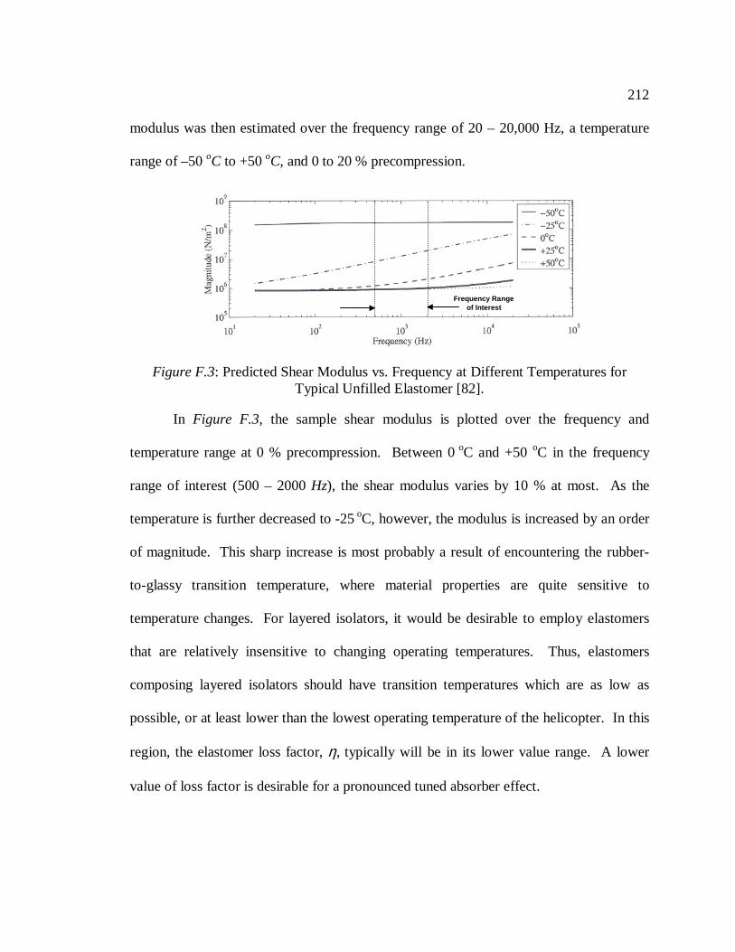
212
modulus was then estimated over the frequency range of 20 – 20,000 Hz, a temperature
range of –50 oC to +50 oC, and 0 to 20 % precompression.
In Figure F.3, the sample shear modulus is plotted over the frequency and
temperature range at 0 % precompression. Between 0 oC and +50 oC in the frequency
range of interest (500 – 2000 Hz), the shear modulus varies by 10 % at most. As the
temperature is further decreased to -25 oC, however, the modulus is increased by an order
of magnitude. This sharp increase is most probably a result of encountering the rubber-
to-glassy transition temperature, where material properties are quite sensitive to
temperature changes. For layered isolators, it would be desirable to employ elastomers
that are relatively insensitive to changing operating temperatures. Thus, elastomers
composing layered isolators should have transition temperatures which are as low as
possible, or at least lower than the lowest operating temperature of the helicopter. In this
region, the elastomer loss factor, η, typically will be in its lower value range. A lower
value of loss factor is desirable for a pronounced tuned absorber effect.
Figure F.3: Predicted Shear Modulus vs. Frequency at Different Temperatures forTypical Unfilled Elastomer [82].
Frequency Rangeof Interest
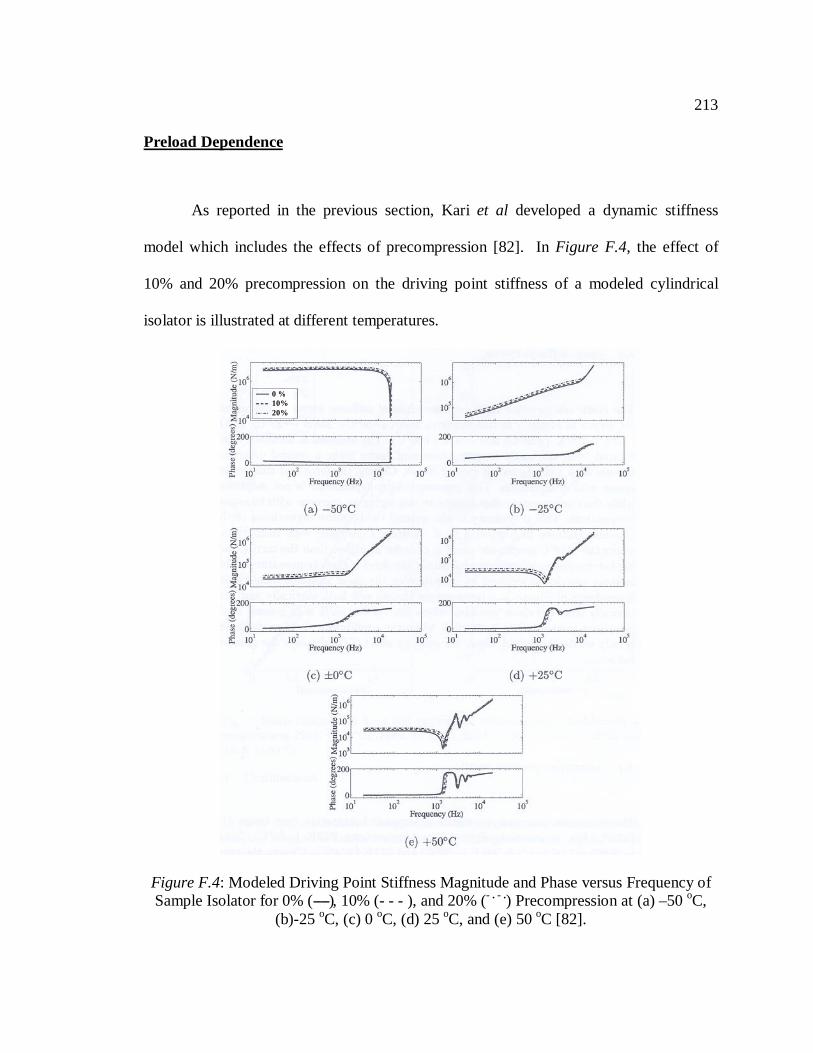
213
Preload Dependence
As reported in the previous section, Kari et al developed a dynamic stiffness
model which includes the effects of precompression [82]. In Figure F.4, the effect of
10% and 20% precompression on the driving point stiffness of a modeled cylindrical
isolator is illustrated at different temperatures.
Figure F.4: Modeled Driving Point Stiffness Magnitude and Phase versus Frequency ofSample Isolator for 0% (----), 10% (- - - ), and 20% (- . - .) Precompression at (a) –50 oC,
(b)-25 oC, (c) 0 oC, (d) 25 oC, and (e) 50 oC [82].
0 %10%20%

214
Driving point stiffness is defined as the driving force divided by the displacement
at one end of the isolator with the other end fixed. As Figure F.4 indicates,
precompression appears to have only a mild effect on isolator stiffness with a maximum
increases of about 20% at 20% precompression. The direct effect of precompression on
shear modulus, however, was not reported. An increase in driving point stiffness,
however, implies an increase in shear modulus at high frequencies.
Frequency Dependence
Figure F.5 indicates the typical relationship between elastomer shear modulus
and frequency. Like temperature dependence plots, rubber, transition, and glassy regions
can be identified. Actual measurements at such high frequencies are difficult to obtain,
and are most often estimated using temperature-frequency shift functions.
In the frequency range of interest (500-2000 Hz), the shear modulus shows little
dependence on frequency. This insensitivity to frequency would be desirable for
elastomers employed in layered isolators.

215
Figure F.5: Unfilled Material Shear Modulus vs. Frequency [79].
Figure F.6: Young’s Modulus versus Reduced Frequency for Rubber Isolator Material[83].

216
The reduced frequency measurements in Figure F.6 of a rubber isolation element
correspond to actual frequencies ranging from 200 to 4000 Hz at the various temperatures
[83]. This experimental data shows that the rubber’s Young’s modulus increases by a
factor of as much as three with increasing frequency.
Like an insensitive temperature dependence, an insensitive frequency dependence
would significantly ease design considerations. Therefore, as Figure F.5 indicates,
elastomers with a relatively high rubber-to-glassy transition frequency should be
employed in layered isolators.
Because isolators are seldom exposed to a single frequency, it is useful to
examine the effects of dual frequency excitation on isolator stiffness properties. In
Figure F.7, isolator stiffness is plotted versus dynamic amplitude for an example isolator.
The solid line indicates the stiffness at 10 Hz with varying amplitude. The dashed line
represents the same conditions with an imposed 1 Hz frequency amplitude. The results
Figure F.7: Stiffness vs. Dynamic Amplitude for Single Frequency and SuperimposedFrequencies for Carbon Black-Filled Isolator [79].

217
suggest that the existence of multiple frequencies can influence the dynamic properties at
a single frequency. Because layered isolators in helicopters would experience a range of
frequency excitations, this effect may need to be considered in layered isolator design.

VITA
Contact InformationOffice Address Home Address229 Hammond Building 1238 Inverary PlaceUniversity Park, PA 16802 State College, PA 16801Phone: 814-865-1986 Email: [email protected]
Phone: 814-234-6654Education
Doctor of Philosophy in Mechanical Engineering, The Pennsylvania State UniversityMasters of Science in Mechanical Engineering, December 2002, The Pennsylvania State UniversityBachelor of Science with High Distinction, University Scholars Program, Mechanical Engineering, May
1997, The Pennsylvania State University
Honors and AwardsAHS Vertical Flight Foundation Scholarship, 2002Rotorcraft Center Fellowship, 1999 and 2000Penn State Honors Program, 1993-1997Phi Beta Kappa Honors Society, 1993-1997National Merit Scholar, 1997
Work ExperienceSummer Internship, Sikorsky Aircraft, 1999Summer Internship, The Ford Motor Company, 1996Mathematics Tutor, Penn State University, 1994-1997
PublicationsSzefi, J.T., Smith, E.C. and Lesieutre, G.A., “Formulation and Validation of a Ritz-based Analytical Model
of High Frequency Periodically Layered Isolators in Compression,” Accepted for Publication in theJournal of Sound and Vibration.
Szefi, J.T., Smith, E.C. and Lesieutre, G.A., “Design, Analysis, and Testing of High-FrequencyPeriodically Layered Isolators with Passive Design Enhancements for Helicopter Gearbox Isolation,”AHS 59th Annual Forum, Phoenix, AZ, 2003.
Szefi, J.T., Smith, E.C. and Lesieutre, G.A., “Design and Analysis of High Frequency Periodically LayeredIsolators for Helicopter Gearbox Isolation,” 44th Structures, Structural Dynamics and MaterialsConference, Norfolk, VA, 2003.
Szefi, J.T., Smith, E.C. and Lesieutre, G.A., “Formulation and Validation of a Ritz-Based Analytical Modelfor Design of Periodically-Layered Isolators in Compression,” 42nd Structures, Structural Dynamicsand Materials Conference, Seattle, WA, 2001.
Szefi, J.T., Smith, E.C. and Lesieutre, G.A., “Analysis and Design of High Frequency Periodically LayeredIsolators in Compression,” 41st Structures, Structural Dynamics and Materials Conference, Atlanta,GA., 2000.