THE PEAK ALGEBRA THE DESCENT ALGEBRAS OF TYPES B AND …

arX

iv:m

ath/

0302

278v

4 [

mat

h.C

O]

2 M

ay 2

003

THE PEAK ALGEBRA

AND

THE DESCENT ALGEBRAS OF TYPES B AND D

MARCELO AGUIAR, NANTEL BERGERON, AND KATHRYN NYMAN

Abstract. We show the existence of a unital subalgebra Pn of the symmetric groupalgebra linearly spanned by sums of permutations with a common peak set, which wecall the peak algebra. We show that Pn is the image of the descent algebra of type Bunder the map to the descent algebra of type A which forgets the signs, and also the

image of the descent algebra of type D. The algebra Pn contains a two-sided ideal◦

Pn

which is defined in terms of interior peaks. This object was introduced in previous workby Nyman [28]; we find that it is the image of certain ideals of the descent algebrasof types B and D introduced in [4] and [9]. We derive an exact sequence of the form

0 →◦

Pn→ Pn → Pn−2 → 0. We obtain this and many other properties of the peak

algebra and its peak ideal by first establishing analogous results for signed permuta-tions and then forgetting the signs. In particular, we construct two new commutativesemisimple subalgebras of the descent algebra (of dimensions n and ⌊n

2⌋+1) by group-

ing permutations according to their number of peaks or interior peaks. We discuss the

Hopf algebraic structures that exist on the direct sums of the spaces Pn and◦

Pnover

n ≥ 0 and explain the connection with previous work of Stembridge [31]; we also obtainnew properties of his descents-to-peaks map and construct a type B analog.

Introduction

A descent of a permutation w ∈ Sn is a position i for which wi > wi+1, while a peak isa position i for which wi−1 < wi > wi+1. The first in-depth study of the combinatorics ofpeaks was carried out by Stembridge [31], who developed an analog of Stanley’s theory ofposet partitions where the notion of descents (of linear extensions of posets) is replacedby the notion of peaks. More recent works uncovered connections between peaks andsuch disparate topics as the generalized Dehn-Sommerville equations [6, 10, 1] and theSchubert calculus of isotropic flag manifolds [11, 8, 7]. Additional interest in the studyof peaks grew from Nyman’s thesis [27, 28], which showed that summing permutationsaccording to their peak sets leads to a non-unital subalgebra of the group algebra of thesymmetric group, much as Solomon’s descent algebra is constructed in terms of descentsets. Work that followed includes [29, 17] and the present paper.Our work developed from the observation that peaks of ordinary permutations are

closely related to descents of signed permutations (permutations of type B). This led

Date: March 3, 2003.2000 Mathematics Subject Classification. Primary 05E99, 20F55; Secondary: 05A99, 16W30.Key words and phrases. Solomon’s descent algebras, peak algebra, signed permutations, Coxeter

groups, types B and D, Hopf algebras.The first author would like to thank Swapneel Mahajan for sharing his insight on descent algebras

and for interesting conversations.Research of the second author supported in part by CRC, NSERC and PREA.

1

http://arxiv.org/abs/math/0302278v4

2 MARCELO AGUIAR, NANTEL BERGERON, AND KATHRYN NYMAN

Contents

Introduction 11. Descent algebras of Coxeter systems 52. Morphisms between descent algebras 73. Peaks of permutations and descents of signed permutations 94. The peak algebra 145. Interior peaks and canonical ideals in types B and D 165.1. The canonical ideal in type B 165.2. The ideal of interior peaks 175.3. From the canonical ideal to the peak ideal 195.4. The canonical ideal in type D 216. Commutative subalgebras of the descent and peak algebras 226.1. Commutative subalgebras of the descent algebra of type B 236.2. From number of descents to number of peaks 246.3. Commutative subalgebras of the peak algebra 256.4. Exact sequences for the commutative subalgebras 276.5. Commutative subalgebras of the descent algebra of type D 287. The algebra of Mantaci and Reutenauer. Right ideals 297.1. Bases of the algebra of Mantaci and Reutenauer 297.2. The image of the algebra of Mantaci and Reutenauer 317.3. The canonical ideal in type B and the peak ideal as principal right ideals 327.4. The descents-to-peaks transform and its type B analog 348. Hopf algebraic structures 378.1. The Hopf algebras of permutations and signed permutations 378.2. The Hopf algebra of non-commutative symmetric functions and its type B analog 388.3. The Hopf algebra of interior peaks and its type B analog 398.4. The module coalgebra of peaks and its type B analog 408.5. Duality. Stembridge’s Hopf algebra 418.6. The action on words 42References 44

us to the discovery of a new object: a unital subalgebra of the descent algebra of thesymmetric group, which we call the peak algebra. This algebra is linearly spanned bysums of permutations with a common set of peaks. The object considered in [28, 29] isthe linear span of the sums of permutations with a common set of interior peaks. Wefind that this is in fact a two-sided ideal of the peak algebra. We warn the reader thatin [28, 29] the terminology “peak algebra” refers to our peak ideal, viewed as a non-unitalalgebra (and our peak algebra is not considered in those works).We obtain several properties of the peak algebra and the peak ideal. Our approach

consists of obtaining more general properties that hold at the level of signed permutationsand then specializing by means of the canonical map that forgets the signs. This allowsfor simpler proofs of known results for the peak ideal, as well as many new propertiesfor both the peak algebra and the peak ideal.We next review the contents of the paper in more detail.Let Sol(An−1), Sol(Bn) and Sol(Dn) denote Solomon’s descent algebras of the Coxeter

systems of types A, B and D (see Section 1 for the basic definitions). Let Sn, Bn andDn be the corresponding Coxeter groups. Sol(An−1) is thus the usual descent algebra ofthe symmetric group Sn.

PEAK AND DESCENT ALGEBRAS 3

In Section 2 we introduce a commutative diagram of morphisms of algebras

Sol(Bn)χ

//

ϕ&&MMMMMMMMMM

Sol(Dn)

ψxxqqqqqqqqqq

Sol(An−1)

The map χ is due to Mahajan [23, 22]. These maps exist at the level of groups (forinstance, ϕ(w) is the permutation obtained by forgetting the signs of the signed per-mutation w), but it is not obvious that they restrict to descent algebras. We provethese facts in Propositions 2.1, 3.2 and 3.6. Central to this is the analysis of the trans-formation of descents of signed permutations under the map ϕ, which we carry out inSection 3. The principle that arises is: peaks are shadows of descents of type B and arenot straightforwardly related to descents of type A.We will show that the images of ϕ and ψ coincide. This common image is a certain

subalgebra of Sol(An−1) whose study is the main goal of this paper. One of our mainresults (Theorem 4.2) states that this subalgebra is linearly spanned by the elements

PF :=∑

Peak(w)=F

w ,

where Peak(w) denotes the set of peaks of a permutation w. We refer to this subalgebraas the peak algebra and denote it by Pn. It is important to note that we allow 1 as apossible peak (by making the convention that w0 = 0).Previous work of Nyman [27, 28] had shown the existence of a similar (but nonunital)

subalgebra of Sol(An−1)—the difference stemming solely from the fact that peaks at 1were not allowed in that work. We obtain a stronger result in this work: we show thatNyman’s algebra is in fact a two-sided ideal of Pn (Theorem 5.7). This ideal, that we

denote by◦

Pn, is the image under ϕ of the two-sided ideal I0n of Sol(Bn) introduced in [4],and also under ψ of a similar ideal of Sol(Dn) introduced in [9]. We obtain these resultsin Theorems 5.9 and 5.12.We describe an exact sequence of the form

0 →◦

Pn → Pn → Pn−2 → 0

and relate it to the exact sequences of [4] and [9] involving the descent algebras of types Band D (Corollary 5.10 and Theorem 5.12). This is an algebraic version of the Fibonaccirecursion fn = fn−1 + fn−2.It is well-known that grouping permutations according to the number of descents leads

to a commutative semisimple subalgebra of Sol(An−1) [21]. In Section 6 we derive ananalogous result for the linear span of the sums of permutations with a given number ofpeaks. Once again, it is possible to easily derive this fact from results for type B, whichare known from [5, 23]. We find (Theorem 6.8) in fact two commutative semisimple

subalgebras ℘n and ℘n of Pn and a two-sided ideal◦℘n of ℘n such that

℘n = ℘n +◦℘n .

In parallel with the situation for the peak algebra and its peak ideal, ℘n and◦℘n are

obtained by grouping permutations according to the number of peaks and interior peaks,

respectively. Thus, we see that◦℘n coincides with the non-unital commutative subalgebra


studied by Schocker [29]. Objects closely related to ℘n and◦℘n were first described by

Doyle and Rockmore [13]. See Remarks 6.9 for more details about these connections.In Corollary 6.12, we describe an exact sequence relating ℘n and ℘n−2 and an analogous

sequence at the level of type B. The corresponding objects at the level of type D arediscussed in Section 6.5.Mantaci and Reutenaer have defined a certain subalgebra of the group algebra of Bn

which strictly contains the descent algebra [26]. We denote it by Sol±(Bn). We recall itsdefinition in Section 7, and provide several new results that link Sol±(Bn) to Sol(An−1)by means of ϕ. The correspondence between types B and A is then summarized by thediagram

I0n

ϕ��

⊆ Sol(Bn)

ϕ

��

⊆ Sol±(Bn)

ϕ��

⊆ QBn

ϕ

��◦

Pn⊆ Pn ⊆ Sol(An−1) ⊆ QSn

We show that I0n is a right ideal of Sol±(Bn) and that it is in fact principal (Corollary 7.7).

This allows us to recover a result of Shocker: that◦

Pn is a principal right ideal of

Sol(An−1) (Corollary 7.8). In addition, we obtain a new result that states that◦

Pn isprincipal as a right ideal of Pn (this result neither implies Schocker’s result nor is itimplied by it), as well as the corresponding statement for type B (Proposition 7.14).

An important map Θ : Sol(An−1) →◦

Pn, which we call the descents-to-peaks transform,is discussed in Section 7.4. We construct a type B analog Θ± : Sol±(Bn) → I0n, fromwhich the basic properties of Θ may be easily derived. The descent-to-peaks transformis a special case of a map considered by Krob, Leclerc and Thibon [20] and is dual to amap considered by Stembridge [31]. See Remarks 7.11 for the precise details.In Section 8 we consider the direct sum over all n ≥ 0 of the group, descent and peak

algebras discussed in previous sections. This leads to a diagram

I0

ϕ��

⊆ Sol(B)

ϕ

��

⊆ Sol±(B)

ϕ��

⊆ QB

ϕ

��◦

P ⊆ P ⊆ Sol(A) ⊆ QS

It is known from work of Malvenuto and Reutenauer [25] that the space QS may beendowed with a new product (called the external product) and a coproduct that turn itinto a graded Hopf algebra. Moreover, this structure restricts to Sol(A), which resultsin the Hopf algebra of non-commutative symmetric functions. Using results from [2],we discuss type B analogs of these constructions and show that all objects in the abovediagram are Hopf algebras, except for Sol(B), which is an I0-module coalgebra, and P,

which is a◦

P-module coalgebra. We also discuss the behavior with respect to the externalstructure of all maps from previous sections.In Section 8.5 we clarify the connection between Stembridge’s Hopf algebra of peaks

and the objects discussed in this paper. The Hopf algebra◦

P and the descents-to-peakstransform are dual to the objects considered by Stembridge in [31].


In Section 8.6 we recall the canonical action of permutations on words, and provide an

explicit description for the action of the generators of the principal ideals I0n and◦

Pn interms of symmetrizers and Jordan brackets (Propositions 8.8 and 8.9). This complementsa result of Krob, Leclerc and Thibon [20].Most of the results in this paper were presented by one of us (Nyman) at the meeting

of the American Mathematical Society in Montreal in May, 2002.

1. Descent algebras of Coxeter systems

Let (W,S) be a finite Coxeter system [18]. That is, W is a finite group generated bythe set S subject to the relations

(st)mst = 1 for all s, t ∈ S ,

where the mst are positive integers and mss = 1 for all s ∈ S.Given w ∈ W , its descent set is

Des(w) := {s ∈ S | ℓ(ws) < ℓ(w)} ,

where ℓ(w) denotes the length of a minimal expression for w as a product of elements ofS.Let QW denote the group algebra of W . The subspace spanned by the elements

(1.1) YJ :=∑

Des(w)=J

w

is closed under the product of QW [30]. It is the Solomon’s descent algebra of (W,S).The unit element is Y∅ = 1.The set {YJ}J⊆S is a linear basis of the descent algebra. A second linear basis is

defined by

(1.2) XJ :=∑

I⊆J

YI =∑

Des(w)⊆J

w .

Note that

(1.3) YJ =∑

I⊆J

(−1)#J−#IXI

so the set {XJ}J⊆S indeed forms a basis. This basis has proved useful in describing thestructure of descent algebras [30, 14, 15, 4, 9] and will be useful in our work as well.Warning: The notations YJ and XJ do not make reference to the Coxeter system,

which will have to be understood from the context. This is particularly relevant in ourwork in which we deal with descent algebras of various Coxeter systems at the sametime.From now on, we assume that the Coxeter system (W,S) is associated to a Coxeter

graph G : S is the set of vertices and mst is the label of the edge joining s and t (2 ifthere is no such edge and 3 is there is an edge with no label, see Figures 1, 2 and 3). Wedenote the descent algebra of this Coxeter system by Sol(G).For the Coxeter graph An−1, the Coxeter group is the symmetric group Sn and the set

of generators consists of the elementary transpositions si = (i, i+1) for i = 1, . . . , n− 1.We identify this set with the set [n−1] := {1, 2, . . . , n−1} via si ↔ i. A permutation wis represented by a sequence w = w1 . . . wn of distinct symbols from the set [n], where


◦

1

◦

2

◦n−2

◦n−1

Figure 1. The Coxeter graph An−1

wi = w(i) are the values of the permutation. A permutation w ∈ Sn has a descent ati ∈ [n−1] if wi > wi+1.

◦4

0

◦

1

◦

2

◦n−2

◦n−1

Figure 2. The Coxeter graph Bn

For the Coxeter graph Bn, the Coxeter group is the group of signed permutationsSn ⋉ Zn2 , which we denote by Bn. A signed permutation w is represented by a sequencew = w1 . . . wn of symbols from 1 to n (the underlying permutation from Sn), some ofwhich may be barred (according to the sign from Zn2 ). We order these symbols by

(1.4) . . . < 2 < 1 < 1 < 2 < . . . .

The set of generators consists of the elementary transpositions si as before (with nosigns) plus the signed permutation

s0 := 12 . . . n .

We identify this set with the set [n−1] := {0} ∪ [n−1]. A signed permutation w ∈ Bnhas a descent at i ∈ [n−1] if wi > wi+1, with respect to the order (1.4), where we agreethat w0 = 0.

◦

FFFFF

FFFF

1

◦

2

◦

3

◦n−2

◦n−1

◦

xxxxxxxxx

1′

Figure 3. The Coxeter graph Dn

For the Coxeter graph Dn, the Coxeter group is the subgroup of Bn consisting of thosesigned permutations with an even number of signs (bars). We denote it by Dn.The set of generators consists of the elementary transpositions si as before, from i = 1

to n−1, plus the signed permutation

s1′ := 213 . . . n .

We identify this set with the set [n−1]′ := {1′} ∪ [n−1].


It is convenient to represent a signed permutation w = w1 . . . wn ∈ Dn by a fork-shapedsequence

w1w2w = w3 · · ·wn−1wn

w1′

of symbols from 1 to n, possibly barred, with the convention that w1′ = w1. It thenturns out that an element w ∈ Dn has a descent at i ∈ [n−1]′ if wi > wi+1, with respectto the order (∗), and where we understand that 1′ + 1 = 2. For instance,

21s1′ = 3 · · · n−1 n

2

has a descent at 1′ because 2 > 1, but not at 1, since 2 < 1.

2. Morphisms between descent algebras

There is a canonical morphism ϕ : Bn ։ Sn from the group of signed permutationsonto that of ordinary permutations, obtained by simply forgetting the signs (bars). Letψ : Dn ։ Sn be its restriction. Consider the linear extensions of these maps to thegroup algebras. We will show in Section 3 that these maps restrict to the correspondingdescent algebras, yielding morphisms of algebras

ϕ : Sol(Bn) → Sol(An−1) and ψ : Sol(Dn) → Sol(An−1) .

It turns out that there is also a morphism of algebras

χ : Sol(Bn) → Sol(Dn)

such that ϕ = ψχ. In this section we concentrate on this map.The map χ is due to Mahajan. It is not the restriction of a morphism of groups

Bn → Dn, and its construction is better understood from the point of view of hyperplanearrangements, as explained in [23, Section 6.1]. We will add a group-theoretic counterpartto Mahajan’s geometric construction that makes the above commutativity evident (butdoes not explain why χ is a morphism of algebras).We begin by defining a map χ : Bn ։ Dn as

χ(w) =

{w if w ∈ Dn ,

ws0 if w /∈ Dn .

In other words, χ changes the sign of the first entry if the number of signs is odd. Notethat χ is not a morphism of groups. Nevertheless, we have the following

Proposition 2.1. The map χ restricts to descent algebras and, at that level, it is amorphism of algebras χ : Sol(Bn) → Sol(Dn). Moreover, it is explicitly given as follows:for J ⊆ {2, . . . , n−1},

YJ 7→ YJ

Y{1}∪J 7→ Y{1′}∪J + Y{1}∪J + Y{1′,1}∪J

Y{0}∪J 7→ YJ + Y{1′}∪J + Y{1}∪J(2.1)

Y{0,1}∪J 7→ Y{1′,1}∪J


or equivalently,

XJ 7→ XJ

X{1}∪J 7→ X{1′,1}∪J

X{0}∪J 7→ X{1′}∪J +X{1}∪J(2.2)

X{0,1}∪J 7→ 2 ·X{1′,1}∪J

Proof. Consider Y{1}∪J ∈ Sol(Bn). Take w ∈ Bn such that Des(w) = {1} ∪ J . There areexactly three possibilities for Des(χ(w)):

if −w1 > w2 then Des(χ(w)) = {1′, 1} ∪ J ,if −w1 < w2 and w ∈ Dn then Des(χ(w)) = {1} ∪ J , andif −w1 < w2 and w /∈ Dn then Des(χ(w)) = {1′} ∪ J .

Conversely, given v ∈ Dn such that Des(v) = {1} ∪ J , we must have v1 > 0; so lettingw = v ∈ Bn we obtain Des(w) = {1} ∪ J and χ(w) = v. If, instead, Des(v) = {1′} ∪ J ,then we must have v1 < 0, so letting w = vs0 ∈ Bn we still obtain Des(w) = {1} ∪ Jand χ(w) = v. Finally, if Des(v) = {1′, 1} ∪ J , then we let w = v ∈ Bn if v1 > 0 andw = vs0 ∈ Bn if v1 < 0, to obtain the same conclusion.Therefore,

χ(Y{1}∪J) = Y{1′}∪J + Y{1}∪J + Y{1′,1}∪J .

The remaining expressions in (2.1) may be similarly deduced. The expressions in (2.2)follow easily from (1.2).Comparing (2.2) to [23, Section 6.1] we see that χ coincides with Mahajan’s map. His

construction guarantees that χ : Sol(Bn) → Sol(Dn) is a morphism of algebras. �

Remark 2.2. It is possible to give a direct proof of the fact that χ is a morphismof algebras by making use of the multiplication rules for the X-bases of Sol(Bn) andSol(Dn) given in [4, Theorem 1] and [9, Theorem 1].

Corollary 2.3. There is a commutative diagram of morphisms of algebras

(2.3) Sol(Bn)χ

//

ϕ&&MMMMMMMMMM

Sol(Dn)

ψxxqqqqqqqqqq

Sol(An−1)

Proof. The commutativity ϕ = ψχ already holds at the level of groups, clearly. �

The descent algebras Sol(Bn) and Sol(Dn) have the same dimension 2n, but the mapχ is not an isomorphism: its image has codimension 2n−2. In fact, the image of χ may

be easily described. Consider the decomposition Dn = D(1)n

∐D

(2)n

∐D

(3)n where the D

(i)n

are respectively defined by the conditions

|w1| < w2, |w1| > |w2| and |w1| < −w2 .

In the group algebra of Dn, define elements

Y(i)J =

∑{w ∈ D(i)

n | Des(w) ∩ {2, . . . , n−1} = J},

for each J ⊆ {2, . . . , n−1} and i = 1, 2, 3.


Corollary 2.4. The image of χ : Sol(Bn) → Sol(Dn) is linearly spanned by the elements

Y(i)J . In particular, these elements span a subalgebra of Sol(Dn) of dimension 3 · 2n−2

(and codimension 2n−2).

Proof. It suffices to observe that

Y(1)J = YJ , Y

(2)J = Y{1′}∪J + Y{1}∪J and Y

(3)J = Y{1′,1}∪J

and to make use of (2.1). �

The maps ϕ and ψ are harder to describe in terms of the Y or X bases. An explicitdescription is provided below (Propositions 3.2, 3.3 and 3.6). It turns out that thesemaps have the same image, even though χ is not surjective. The main goal of this paperis to describe this image, a certain subalgebra of Sol(An−1), in explicit combinatorialterms.

Remark 2.5. A similar commutative diagram to (2.3) is given in [23, Section 6]. In fact,the map χ is the same for both, but the maps Sol(Bn) → Sol(An−1) and Sol(Dn) →Sol(An−1) considered in [23] are different from ours.

3. Peaks of permutations and descents of signed permutations

Definition 3.1. Let w ∈ Sn. The set of peaks of w is

Peak(w) = {i ∈ [n−1] | wi−1 < wi > wi+1} ,

where we agree that w0 = 0.

For instance, Peak(42153) = {1, 4}. Note that 1 is a peak of w if and only if it is adescent of w. Thus, our notion of peaks differs (slightly) from that of [31, 28, 29]. Thisturns out to be an important distinction, as will be made clear throughout this work.We will deal with both notions of peaks starting in Section 5.Let Qn denote the collection of all subsets of [n−1], and

Fn = {F ∈ Qn | if i ∈ F then i+ 1 /∈ F}.

Throughout this work, by the n-th Fibonacci number we understand

(3.1) fn := #Fn .

Thus, f0 = 1, f1 = 1, f2 = 2 and fn = fn−1 + fn−2.Clearly, the peak set of any permutation w ∈ Sn belongs to Fn. It is easy to see that

any element of Fn is realized in this way.Given J ∈ Qn, consider the set

Λ(J) := {i ∈ J | i− 1 /∈ J}.

One verifies immediately that Λ(J) ∈ Fn and, moreover, that the diagram

(3.2) SnDes~~}}

}}Peak A

AAA

QnΛ

//Fn

commutes.For each F ∈ Fn, define an element of the group algebra of Sn by

(3.3) PF :=∑

Peak(w)=F

w .


It follows from (1.1) and (3.2) that

(3.4) PF =∑

Λ(J)=F

YJ ;

in particular, each PF belongs to the descent algebra Sol(An−1).It turns out that ϕ : Sol(Bn) → Sol(An−1) maps a basis element YJ to a certain sum

of elements PF . In order to derive an explicit expression for ϕ(YJ), we need to introducesome notation and make some basic observations.First, given a permutation u ∈ Sn and a position i ∈ [n], we refer to one of the four

diagrams◦??

◦??◦,

◦��◦

��◦, ◦?? ◦

◦�� , ◦??

◦�� ◦

as the local shape of u at i, according to whether ui−1 > ui > ui+1, ui−1 < ui < ui+1,ui−1 > ui < ui+1 or ui−1 < ui > ui+1, respectively. Here, we make the conventions thatu0 = 0 and un+1 = +∞. A position i is a peak of u if the local shape at i is ◦??

◦�� ◦ ; we

also say that i is a valley if the local shape is ◦?? ◦◦

�� . Note that valleys may only occurin positions 2, . . . , n, while peaks only in positions 1, . . . , n−1. Note also that the totalnumber of peaks equals the total number of valleys, since in listing them from left toright, peaks and valleys alternate, starting always with a peak and ending with a valley(except for the case of the identity permutation, which has no peaks or valleys). Forinstance, the four local shapes for u = 2413 are, from left to right,

◦��◦

��◦, ◦??

◦�� ◦ ,

◦?? ◦◦�� and

◦��◦

��◦.

Similarly, for a signed permutation w ∈ Bn and i ∈ [n], we speak of its local shape ati, which is one of the previous diagrams decorated by the sign of the entry wi, with thesame conventions. For instance, the four local shapes of w = 2413 are (in order)

◦??+

◦�� ◦

,◦?? ◦

��◦−

, ◦??+

◦�� ◦

and◦

��◦��+

◦.

Clearly, the collection of all local shapes of w ∈ Bn determine its descent set, andconversely. More precisely, given a subset J ⊆ [n−1], we have that Des(w) = J if andonly if for each i ∈ [n], the local shape of w at i is as follows

◦??◦??±

◦◦??±

◦�� ◦

◦?? ◦��◦

±

◦��◦

��±

◦(A)

i∈J, i∈J+1 i∈J, i/∈J+1 i/∈J, i∈J+1 i/∈J, i/∈J+1

where J + 1 denote the shifted set J + 1 = {i+ 1 | i ∈ J}.Now suppose that a permutation u ∈ Sn is given and we look for all 2n signed per-

mutations w ∈ Bn such that ϕ(w) = u. Given a local shape of u at i ∈ [n], the possiblelocal shapes of w at i are as follows

(B)

u ∈ Sn w ∈ Bn , ϕ(w) = u◦??

◦??◦

◦??◦??+

◦

◦��◦

��−

◦

◦?? ◦��◦

−◦??+

◦�� ◦

◦��◦

��◦

◦??◦??−

◦

◦��◦

��+

◦

◦?? ◦��◦

−◦??+

◦�� ◦

◦?? ◦◦

��◦??

◦??±

◦

◦��◦

��±

◦

◦?? ◦��◦

±◦??±

◦�� ◦

◦??◦�� ◦

◦?? ◦��◦

−◦??+

◦�� ◦


Let I △ J = (I ∪ J) \ (I ∩ J) be the symmetric set difference.

Proposition 3.2. The map ϕ : Sol(Bn) → Sol(An−1) is explicitly given by

(3.5) YJ 7→∑

F∈Fn

F⊆J△(J+1)

2#F · PF ,

for any J ⊆ [n−1].

Proof. We need to show that for each u ∈ Sn,(∗)

#{w ∈ Bn | Des(w) = J and ϕ(w) = u} =

{2#Peak(u) if Peak(u) ⊆ J △ (J + 1) ,

0 if not.

Note that this set is defined precisely by conditions (A) and (B) above.Suppose there is at least one w in the above set and take i ∈ Peak(u). By (B), the

local shape of w at i is either◦?? ◦

��◦−

or ◦??+

◦�� ◦

. Then, by (A), i ∈ J △ (J + 1). This proves

the second half of (∗).Assume now that Peak(u) ⊆ J △ (J + 1). A signed permutation w in the above set is

completely determined once the signs of its entries |wi| = ui are chosen. We will showthat the signs at those positions i that are valleys of u can be freely chosen, while thesigns at the remaining positions are uniquely determined. This proves the remaining halfof (∗), because as explained above, the number of valleys equals the number of peaks, sothe number of such choices is 2#Peak(u).Given a position i, it will fall into one of the four alternatives of (A) (according to

J) and one of the four alternatives of (B) (according to u). Consider first the case of aposition i that is not a valley of u. In this case, whatever the alternative in (A) is, thereis exactly one possible local shape for w that satisfies (B). In particular, the sign of wiis uniquely determined for all those positions i. On the other hand, if i is a valley of u,then whatever the alternative in (A) is, there are exactly two possible local shapes forw that satisfy (B), each with the same underlying shape but with different signs. Thus,the choices of signs that lead to a signed permutation w that satisfies (A) and (B) is thesame as the choices of signs on the set of valleys of u, as claimed. �

We can derive a similar expression for ϕ on the X-basis of Sol(Bn).

Proposition 3.3. The map ϕ : Sol(Bn) → Sol(An−1) is explicitly given by

(3.6) XJ 7→ 2#J ·∑

F∈Fn

F⊆J∪(J+1)

PF

for any J ⊆ [n−1].

Proof. Since XJ =∑

K⊆J YK , equation (3.6) will follow from (3.5), once we show that

for any F ∈ Fn and J ⊆ [n−1] we have

#{K ⊆ [n−1] | F ⊆ K △ (K + 1), K ⊆ J} =

{2#J−#F if F ⊆ J ∪ (J + 1),

0 if not.


If there is at least one subset K in the above family, then F ⊆ K∪ (K+1) ⊆ J ∪ (J+1).This proves the second case of the equality.Suppose now that F ⊆ J ∪ (J + 1). We decompose an arbitrary subset K of J into

five pieces:

K0 := K ∩(J \

(F ∪ (F − 1)

)), K+ := K ∩ F and K− := K ∩ (F − 1) ,

K+1 := K ∩ F ∩ (J + 1) , K+

2 := K ∩ F ∩ (J + 1)c ,

K−1 := K ∩ (F − 1) ∩ (J − 1) , K−

2 := K ∩ (F − 1) ∩ (J − 1)c .

Thus, K = K0⊔K+1 ⊔K

+2 ⊔K

−1 ⊔K−

2 . One may check that, under the present assumptions(F ∈ Fn and F ⊆ J ∪ (J + 1)), a subset K of J satisfies F ⊆ K △ (K +1) if and only ifthe following conditions hold:

K+2 = J∩F ∩(J+1)c , K−

2 = J∩(F−1)∩(J−1)c and K+1 ⊔(K−

1 +1) = J∩F ∩(J+1) ,

while K0 may be any subset of J \(F ∪ (F − 1)

)and K+

1 any subset of J ∩F ∩ (J +1).The claim now follows from the fact that

#J \(F ∪ (F − 1)

)+#J ∩ F ∩ (J + 1) = #J −#F

(this also makes use of the assumptions F ∈ Fn and F ⊆ J ∪ (J + 1)). �

Remark 3.4. Formulas (3.5) and (3.6) are very similar to certain expressions for a mapintroduced by Stembridge [31, Propositions 2.2, 3.5]. This is in fact a consequence of avery non-trivial fact: that the dual of Stembridge’s map admits a type B analog and ϕcommutes with these maps. This connection will be clarified in Sections 7.4 and 8.5.

Remark 3.5. It is interesting to note that for any J ⊆ [n−1],

ϕ(YJ) = ϕ(Y[n−1]\J ) .

This can be deduced from the explicit formula (3.5), but it can also be understood asfollows. Consider the map σ : Bn → Bn which reverses the sign of all the entries of asigned permutation (σ is both left and right multiplication by 12 . . . n). Clearly,

Des(σ(w)

)= [n−1] \Des(w) , and therefore σ(YJ) = Y[n−1]\J .

On the other hand, since ϕ simply forgets the signs, we have

ϕ(w) = ϕ(σ(w)

), and therefore ϕ(YJ) = ϕ

(σ(YJ)

)= ϕ(Y[n−1]\J) .

The map ψ : Sol(Dn) → Sol(An−1) also sends basis elements YJ and XJ to sums ofelements PF . The next result provides explicit expressions.We make use of the convention 1′ + 1 = 2 to give meaning to the shifted set J + 1 =

{i+ 1 | i ∈ J}, where J is any subset of [n−1]′.


Proposition 3.6. The map ψ : Sol(Dn) → Sol(An−1) is explicitly given by

YJ 7→∑

F∈Fn

F⊆J△(J+1)

2#F · PF

Y{1}∪J and Y{1′}∪J 7→∑

{1}∪F∈Fn

F⊆J△(J+1)

2#F · P{1}∪F(3.7)

Y{1′,1}∪J 7→∑

F∈Fn

F⊆J△({2}∪(J+1)

)2#F · PF

and also

XJ 7→ 2#J ·∑

F∈Fn

F⊆J∪(J+1)

PF

X{1}∪J and X{1′}∪J 7→ 2#J ·∑

F∈Fn

F⊆J∪(J+1)∪{1}

PF(3.8)

X{1′,1}∪J 7→ 2#J+1 ·∑

F∈Fn

F⊆J∪(J+1)∪{1,2}

PF

for any J ⊆ {2, . . . , n−1}.

Proof. It is possible to derive these expressions by a direct analysis of how the notion ofdescents of type D transforms after forgetting the signs, as we did for the type B casein Proposition 3.2. We find it much easier, however, to derive these from the analogousexpressions for the type B case, by means of the commutativity of diagram (2.3).If J ⊆ {2, . . . , n−1}, then by Proposition 2.1, the map χ : Sol(Bn) → Sol(Dn) satisfies

χ(YJ) = YJ . Therefore, by Corollary 2.3 and Proposition 3.2,

ψ(YJ) = ϕ(YJ) =∑

F∈Fn

F⊆J△(J+1)

2#F · PF .

This is the first formula in (3.7). Similarly, the last formula in (3.7) follows from thefacts that χ(Y{0,1}∪J) = Y{1′,1}∪J and

({0, 1} ∪ J

)△

(({0, 1} ∪ J

)+ 1

)= {0} ∪

(J △

({2} ∪ (J + 1)

))

(note that {0} does not affect the summation over subsets F ∈ Fn).The formulas for Y{1}∪J and Y{1′}∪J require a little extra work. First, from Proposi-

tion 2.1 we know that

χ(Y{0}∪J − YJ) = Y{1′}∪J + Y{1}∪J ;

hence, by Corollary 2.3,

ψ(Y{1′}∪J + Y{1}∪J ) = ϕ(Y{0}∪J − YJ) .


Now, since J ⊆ {2, . . . , n − 1}, ({0} ∪ J) △(({0} ∪ J) + 1

)= {0, 1} ∪

(J △ (J + 1)

).

Therefore, by Proposition 3.2,

ϕ(Y{0}∪J − YJ) =∑

F∈Fn

F⊆{1}∪(J△(J+1)

)2#F · PF −

∑

F∈Fn

F⊆J△(J+1)

2#F · PF

=∑

{1}∪F∈Fn

F⊆J△(J+1)

21+#F · P{1}∪F .

Thus, to obtain the expressions in (3.7) for Y{1}∪J and Y{1′}∪J , we only need to show that

ψ(Y{1}∪J) = ψ(Y{1′}∪J) .

This may be seen as follows. Consider the involution ρ : Dn → Dn given by rightmultiplication with the element 123 . . . n. In other words, ρ(w) is obtained from w byreversing the sign of both w1 and w2. Note that w has a descent at 1 but not at1′ if and only if w1 > |w2|, while w has a descent at 1′ but not at 1 if and only if−w1 > |w2|. Therefore, ρ restricts to a bijection between {w ∈ Dn | Des(w) = {1} ∪ J}and {w ∈ Dn | Des(w) = {1′} ∪ J}, for any J ⊆ {2, . . . , n − 1}. Also, since ψ simplyforgets the signs, ψρ = ψ. Therefore, ψ(Y{1}∪J) = ψ(Y{1′}∪J). This completes the proofof (3.7). Formulas (3.8) can be obtained similarly, by making use of Proposition 3.3. �

4. The peak algebra

Definition 4.1. The peak algebra Pn is the subspace of the descent algebra Sol(An−1)linearly spanned by the elements {PF}F∈Fn

defined by (3.3) or (3.4).

We will show below that Pn is indeed a unital subalgebra of Sol(An−1). As explainedin the Introduction, this differs from the object considered in [28, 29]. The connectionbetween the two will be clarified in Section 5.Since the elements PF are sums over disjoint classes of permutations, they are linearly

independent. Thus, they form a basis of Pn and

dimPn = fn ,

the n-th Fibonacci number as in (3.1).The following is one of the main results of this paper.

Theorem 4.2. Pn is a subalgebra of the descent algebra of the symmetric group Sn.Moreover, it coincides with the image of the map ϕ : Sol(Bn) → Sol(An−1) and also withthat of ψ : Sol(Dn) → Sol(An−1).

Proof. Since ϕ and ψ are morphisms of algebras, it is enough to show that their imagescoincide with Pn. We already know that

Im(ϕ) ⊆ Im(ψ) ⊆ Pn

from Proposition 3.6 and Corollary 2.3. We will show that ϕ : Sol(Bn) → Pn is in factsurjective.Define an order on the subsets in Fn by declaring that E < F if the maximum element

in the set E △ F is an element of F . According to Lemma 4.3 (below), this a total order.


For each E ∈ Fn consider the shifted set E − 1 ⊆ [n−1]. We first show that PF doesnot appear in the sum ϕ(XE−1) for any E < F . Let a be the maximum element inE △ F . By the choice of the total order, a ∈ F and a /∈ E. Suppose a ∈ E − 1. Thena+1 ∈ E, and since a is the maximum element of E △ F , we would have a+1 ∈ F . Butthen both a and a + 1 ∈ F , which contradicts the fact that F ∈ Fn. Thus, a /∈ E − 1,and hence F 6⊆ (E − 1) ∪ E. It follows from (3.6) that PF does not appear in the sumϕ(XE−1) for any E ∈ Fn, E < F , while it does appear in ϕ(XF−1). In other words,the matrix of the restriction of ϕ to the subspace of Sol(Bn) spanned by the elements{XF−1 | F ∈ Fn} is unitriangular (with respect to the chosen total order). In particular,ϕ is surjective. �

Lemma 4.3. The relation E < F ⇐⇒ max(E △ F ) ∈ F defines a total order on thefinite subsets of any fixed totally ordered set.

Proof. Let X be the totally ordered set. Encode subsets E of X as sequences xE ∈ ZX2 inthe standard way. Then xE△F = xE + xF . Therefore, the relation E < F corresponds tothe right lexicographic order on ZX2 (defined from 0 < 1 in Z2), which is clearly total. �

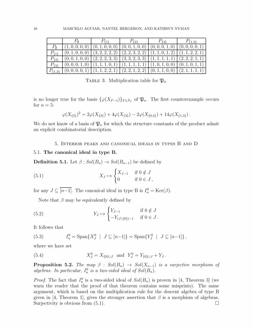
Since the elements PF consist of sums over disjoint classes of permutations, the struc-ture constants for the multiplication of Pn on this basis are necessarily non-negative.Tables 1-4 describe the multiplication for the first peak algebras. The structure con-stants for the product PF ·PG are found at the intersection of the row indexed by PF andthe column indexed by PG, and they are given in the same order as the rows or columns.For instance, in P4,

P{2} · P{1} = 2P∅ + 2P{1} + 2P{2} + 3P{3} + 3P{1,3} .

Note that the peak algebras are not commutative in general.

P∅ P{1}

P∅ (1, 0) (0, 1)P{1} (0, 1) (1, 0)

Table 1. Multiplication table for P2.

P∅ P{1} P{2}

P∅ (1, 0, 0) (0, 1, 0) (0, 0, 1)P{1} (0, 1, 0) (2, 1, 2) (1, 1, 1)P{2} (0, 0, 1) (1, 1, 1) (1, 1, 0)


Remark 4.4. The proof of Theorem 4.2 shows that the set {ϕ(XF−1)}F∈Fnis a basis

of Pn. The structure constants for the product of Sol(Bn) on the basis {XJ}J⊆[n−1] are

non-negative and in fact admit an explicit combinatorial description [4]. However, this


P∅ P{1} P{2} P{3} P{1,3}

P∅ (1, 0, 0, 0, 0) (0, 1, 0, 0, 0) (0, 0, 1, 0, 0) (0, 0, 0, 1, 0) (0, 0, 0, 0, 1)P{1} (0, 1, 0, 0, 0) (3, 2, 2, 2, 2) (2, 2, 3, 2, 2) (1, 1, 0, 1, 2) (1, 1, 2, 2, 1)P{2} (0, 0, 1, 0, 0) (2, 2, 2, 3, 3) (3, 3, 2, 3, 3) (1, 1, 1, 1, 1) (2, 2, 2, 1, 1)P{3} (0, 0, 0, 1, 0) (1, 1, 1, 0, 1) (1, 1, 1, 1, 1) (1, 0, 1, 0, 0) (0, 1, 0, 1, 1)P{1,3} (0, 0, 0, 0, 1) (1, 1, 2, 2, 1) (2, 2, 1, 2, 2) (0, 1, 1, 0, 0) (2, 1, 1, 1, 1)


is no longer true for the basis {ϕ(XF−1)}F∈Fnof Pn. The first counterexample occurs

for n = 5:

ϕ(X{2})2 = 2ϕ(X{2}) + 4ϕ(X{3})− 2ϕ(X{0,3}) + 14ϕ(X{1,3}) .

We do not know of a basis of Pn for which the structure constants of the product admitan explicit combinatorial description.

5. Interior peaks and canonical ideals in types B and D

5.1. The canonical ideal in type B.

Definition 5.1. Let β : Sol(Bn) → Sol(Bn−1) be defined by

(5.1) XJ 7→

{XJ−1 if 0 /∈ J

0 if 0 ∈ J ,

for any J ⊆ [n−1]. The canonical ideal in type B is I0n = Ker(β).

Note that β may be equivalently defined by

(5.2) YJ 7→

{YJ−1 if 0 /∈ J

−Y(J\{0})−1 if 0 ∈ J .

It follows that

(5.3) I0n = Span{X0J | J ⊆ [n−1]} = Span{Y 0

J | J ⊆ [n−1]} ,

where we have set

(5.4) X0J = X{0}∪J and Y 0

J = Y{0}∪J + YJ .

Proposition 5.2. The map β : Sol(Bn) → Sol(Xn−1) is a surjective morphism ofalgebras. In particular, I0n is a two-sided ideal of Sol(Bn).

Proof. The fact that I0n is a two-sided ideal of Sol(Bn) is proven in [4, Theorem 3] (wewarn the reader that the proof of that theorem contains some misprints). The sameargument, which is based on the multiplication rule for the descent algebra of type Bgiven in [4, Theorem 1], gives the stronger assertion that β is a morphism of algebras.Surjectivity is obvious from (5.1). �


5.2. The ideal of interior peaks.

Definition 5.3. Let w ∈ Sn. The set of interior peaks of w is◦

Peak(w) = {i ∈ {2, . . . , n− 1} | wi−1 < wi > wi+1} .

Thus,

(5.5) Peak(w) =

{1} ∪

◦

Peak(w) if 1 ∈ Des(w),◦

Peak(w) if not.

Let◦

Fn be the collection of those F ∈ Fn for which 1 /∈ F . For any w ∈ Sn,◦

Peak(w) ∈◦

Fn,

and it is easy to see that any F ∈◦

Fn can be realized in this way.

For each F ∈◦

Fn, define an element of the group algebra of Sn by

(5.6)◦

P F :=∑

◦

Peak(w)=F

w .

These are the elements considered in Nyman’s original work [28] and also in Schocker’s [29].

The operator◦

Λ(J) := {i ∈ J | i 6= 1, i− 1 /∈ J} satisfies◦

Λ(Des(w)) =◦

Peak(w); thus,we also have

(5.7)◦

P F :=∑

◦

Λ(J)=F

YJ .

Note that if F ∈◦

Fn and 2 /∈ F then {1} ∪ F ∈ Fn.

Lemma 5.4. For any F ∈◦

Fn,

(5.8)◦

P F =

{PF if 2 ∈ F

PF + P{1}∪F if 2 /∈ F .

Proof. Consider first the case when 2 ∈ F . Then, for any w ∈ Sn with◦

Peak(w) = F ,

w1 < w2 > w3; in particular, 1 /∈ Des(w). Hence Peak(w) =◦

Peak(w) and it follows

from (3.3) and (5.6) that PF =◦

PF .

If 2 /∈ F , then the class of permutations w ∈ Sn with◦

Peak(w) = F splits into twoclasses, according to whether they have a descent at 1 or not. In view of (5.5), the firstclass consists of all those w for which Peak(w) = {1} ∪ F , and the second of those for

which Peak(w) = F ; whence◦

P F = P{1}∪F + PF . �

Definition 5.5. The peak ideal◦

Pn is the subspace of Pn linearly spanned by the

elements {◦

PF}F∈

◦

Fn

.

We will show below that◦

Pn is indeed a two-sided ideal of Pn. In particular, it follows

that◦

Pn is closed under the product of Sol(An−1). In [28, 29],◦

Pn is regarded as a non


unital subalgebra of Sol(An−1) (and it is referred to as the peak algebra). The presentwork reveals the existence of the larger unital subalgebra Pn of Sol(An−1), as well as the

extra structure of◦

Pn as an ideal of Pn.First, consider the map π : Pn → Pn−2 defined by

(5.9) PF 7→

PF−2 if neither 1 nor 2 belong to F

−PF\{1}−2 if 1 ∈ F

0 if 2 ∈ F

for any F ∈ Fn. Note that (5.9) covers all possibilities, since 1 and 2 cannot belong toF simultaneously. For the same reason, if 1 ∈ F , the set F \ {1} − 2 belongs to Fn−2.As we will see below (Remark 5.11), the map β : Sol(Bn) → Sol(Bn−1) does not

descend to peak algebras. However, the composite

(5.10) β2 : Sol(Bn)β−→ Sol(Bn−1)

β−→ Sol(Bn−2) , XJ 7→

{XJ−2 if 0, 1 /∈ J

0 if 0 or 1 ∈ J

does. Indeed, it descends precisely to the map π of (5.9).

Proposition 5.6. The map π : Pn → Pn−2 is a surjective morphism of algebras. More-over, there is a commutative diagram

Sol(Bn)β2

//

ϕ

��

Sol(Bn−2)

ϕ

��Pn π

// Pn−2

Proof. It suffices to show that the diagram commutes. That π is a surjective morphismof algebras follows, since so are ϕ and β (Theorem 4.2 and Proposition 5.2).

Take J ⊆ [n−1]. Suppose first that 0 or 1 ∈ J , so that β2(XJ) = 0. In this case,1 ∈ J ∪ (J + 1) and hence

πϕ(XJ)(3.6)= 2#J ·

∑

F∈Fn

F⊆J∪(J+1)

π(PF )

(5.9)= 2#J ·

∑

F∈Fn

F⊆J∪(J+1)

1/∈F,2/∈F

PF−2 − 2#J ·∑

F∈Fn

F⊆J∪(J+1)

1∈F,2/∈F

PF\{1}−2

= 2#J ·∑

F∈Fn

F⊆J∪(J+1)

1/∈F,2/∈F

PF−2 − 2#J ·∑

F ′∈Fn

F ′⊆J∪(J+1)

1/∈F ′,2/∈F ′

PF ′−2 = 0 .

Consider now the case when 0, 1 /∈ J . In this case,

ϕβ2(XJ) = ϕ(XJ−2)(3.6)= 2#J ·

∑

F∈Fn

F⊆(J−2)∪(J−1)

PF ,


since the cardinal of the shifted set J − 2 coincides with the cardinal of J . On the otherhand, since 1 /∈ J ∪ (J + 1), we have

πϕ(XJ)(3.6)= 2#J ·

∑

F∈Fn

F⊆J∪(J+1)

π(PF )(5.9)= 2#J ·

∑

F∈Fn

F⊆J∪(J+1)

1,2/∈F

PF−2 = 2#J ·∑

F∈Fn

F⊆(J−2)∪(J−1)

PF .

Thus, ϕβ2(XJ) = πϕ(XJ) and the proof is complete. �

Since the elements◦

PF are sums over disjoint classes of permutations, they are linearly

independent. Thus, they form a basis of◦

Pn and

dim◦

Pn = #◦

Fn = #Fn−1 = fn−1 ,

the (n− 1)-th Fibonacci number as in (3.1).We can now derive the main result of the section. It may be viewed as an algebraic

counterpart of the recursion fn = fn−1 + fn−2.

Theorem 5.7.◦

Pn is a two-sided ideal of Pn. Moreover, for n ≥ 2,

Pn/◦

Pn∼= Pn−2 .

(For n ≤ 1, we have P0 = P1 =◦

P1 = Q.)

Proof. We know from Proposition 5.6 that π is surjective. Therefore

Pn/Ker(π) ∼= Pn−2 .

To complete the proof of the theorem it suffices to show that

Ker(π) =◦

Pn .

Since dimPn = fn, we have

dimKer(π) = fn − fn−2 = fn−1 = dim◦

Pn .

On the other hand, from (5.8) and (5.9) we immediately see that◦

Pn ⊆ Ker(π). �

5.3. From the canonical ideal to the peak ideal. Let I0,1n denote the kernel of themap β2. Thus, I0,1n is another ideal of Sol(Bn) and I0n ⊆ I0,1n . Moreover, from (5.1)and (5.10) we see that

(5.11) I0,1n = Span{XJ | 0 or 1 ∈ J, J ⊆ [n−1]} .

We will show below that the ideal I0n and the larger ideal I0,1n both map onto◦

Pn. First,we provide an explicit formula for the map ϕ in terms of the bases {X0

J}J⊆[n−1] and

{Y 0J }J⊆[n−1] of I

0n and {

◦

PF}F∈

◦

Fn

of◦

Pn. These turn out to be completely analogous to

the formulas in Propositions 3.2 and 3.3.


Proposition 5.8. For any J ∈ [n−1],

(5.12) ϕ(X0J) = 21+#J ·

∑

F∈◦

Fn

F⊆J∪(J+1)

◦

PF and ϕ(Y 0J ) =

∑

F∈◦

Fn

F⊆J△(J+1)

21+#F ·◦

PF .

Proof. By Proposition 3.3 we have

1

21+#J· ϕ(X{0}∪J ) =

∑

F∈Fn

F⊆{1}∪J∪(J+1)

PF

=∑

1/∈F∈Fn

2∈F⊆J∪(J+1)

PF +∑

1∈F∈Fn

2/∈F⊆{1}∪J∪(J+1)

PF +∑

1/∈F∈Fn

2/∈F⊆{1}∪J∪(J+1)

PF

(5.8)=

∑

F∈◦

Fn

2∈F⊆J∪(J+1)

◦

PF +∑

F ′∈Fn

1,2/∈F ′⊆J∪(J+1)

P{1}∪F ′ +∑

F∈Fn

1,2/∈F⊆J∪(J+1)

PF

=∑

F∈◦

Fn

2∈F⊆J∪(J+1)

◦

P F +∑

F∈Fn

1,2/∈F⊆J∪(J+1)

P{1}∪F + PF

(5.8)=

∑

F∈◦

Fn

2∈F⊆J∪(J+1)

◦

PF +∑

F∈◦

Fn

2/∈F⊆J∪(J+1)

◦

P F

=∑

F∈◦

Fn

F⊆J∪(J+1)

◦

PF .

The formula for Y 0J can be similarly deduced from Proposition 3.2, or from the formula

for X0J , as in the proof of Proposition 3.3. �

Theorem 5.9. ϕ(I0,1n ) = ϕ(I0n) =◦

Pn.

Proof. We already know that ϕ(I0n) ⊆ ϕ(I0,1n ) ⊆◦

Pn. In fact, the first inclusion is trivial

and the second follows from Proposition 5.6, since I0,1n = Ker(β2) and◦

Pn = Ker(π), asseen in the proof of Theorem 5.7.

To complete the proof, we show that ϕ : I0n →◦

Pn is surjective. For each E ∈◦

Fn,consider the element X0

E−1 ∈ I0n. By Proposition 5.8,

ϕ(X0E−1) = 21+#E ·

∑

F∈◦

Fn

F⊆(E−1)∪E

◦

P F .

As in the proof of Theorem 4.2, it follows that◦

P F does not appear in ϕ(X0E−1) for any

E < F , where E < F denotes the total order of Lemma 4.3. On the other hand,◦

PF does


appear in ϕ(X0F−1). Therefore, the matrix of the map ϕ restricted to the subspace of I0n

spanned by the elements X0E−1 is unitriangular. Hence, ϕ : I0n →

◦

Pn is surjective. �

The following corollary summarizes the results that relate the peak algebra and thepeak ideal to the descent algebras of type B.

Corollary 5.10. There is a commutative diagram

0 // I0,1n�

�

//

ϕ��

Sol(Bn)β2

//

ϕ

��

Sol(Bn−2)

ϕ

��

// 0

0 // ◦

Pn

�

�

// Pn π// Pn−2

// 0

where the rows are exact and the vertical maps are surjective.

Proof. The surjectivity of the vertical maps was obtained in Theorems 4.2 and 5.9. Theexactness of the first row is clear from the definitions of β and I0,1n . In the course of the

proof of Theorem 5.7 we obtained that Ker(π) =◦

Pn. Finally, Proposition 5.6 gave thesurjectivity of π and the commutativity of the square. �

Remark 5.11. There is no morphism of algebras Pn → Pn−1 fitting in a commutativediagram

Sol(Bn)β

//

ϕ

��

Sol(Bn−1)

ϕ

��Pn

//_____ Pn−1

For, such a map would be surjective, since so are ϕ and β, and hence its kernel wouldhave dimension dimPn − dimPn−1 = fn−2. But this kernel must contain

ϕ(Ker(β)) = ϕ(I0n) =◦

Pn (by Theorem 5.9)

which has dimension fn−1, a contradiction.

5.4. The canonical ideal in type D. There are similar results relating peaks to thedescent algebras of type D. We present them in this section.Consider the map γ : Sol(Dn) → Sol(Bn−2) defined by

(5.13) XJ 7→

{XJ−2 if 1, 1′ /∈ J

0 if 1 or 1′ ∈ J .

It follows from the proof of Theorem 2 in [9] that γ is a morphism of algebras. Moreover,it is clear from equations (2.2), (5.1) and (5.13) that the diagram

(5.14) Sol(Bn)χ

//

β2 &&MMMMMMSol(Dn)

γxxqqqqqq

Sol(Bn−2)

commutes.Let I1

′,1n denote the kernel of the map γ, an ideal of Sol(Dn). From (5.13) we see that

(5.15) I1′,1n = Span{XJ | 1′ or 1 ∈ J, J ∈ [n−1]′} .


The following theorem describes the relationship between the peak algebra and thepeak ideal to the descent algebras of type D and B.

Theorem 5.12. There is a commutative diagram

0 // I1′,1n

�

�

//

ψ��

Sol(Dn)γ

//

ψ

��

Sol(Bn−2)

ϕ

��

// 0

0 // ◦

Pn

�

�

// Pn π// Pn−2

// 0


Proof. The exactness of the first row is clear from the definitions of γ and I1′,1n . The

second row is exact according to Corollary 5.10.The commutativity of the square

Sol(Dn)γ

//

ψ

��

Sol(Bn−2)

ϕ

��Pn π

// Pn−2

can be shown in the same way as in Proposition 5.6. Together with (5.14), this allowsus to construct a commutative diagram

0 // I0,1n�

�

//

χ

��

Sol(Bn)β2

&&MMMMMMMMMMM

χ

��

0 // I1′,1n

�

�

//

ψ��

Sol(Dn)γ

//

ψ

��

Sol(Bn−2)

ϕ

��

// 0

0 // ◦

Pn

�

�

// Pn π// Pn−2

// 0

Since by Theorem 5.9 the map I0,1n →◦

Pn is surjective, so must be the map I1′,1n →

◦

Pn.This completes the proof. �

6. Commutative subalgebras of the descent and peak algebras

Grouping permutations according to the number of descents leads to the followingelements of the descent algebra of type A:

yj :=∑

u∈Sn

#Des(u)=j

u =∑

J⊆[n−1]

#J=j

YJ ,

for j = 0, . . . , n − 1. It was shown by Loday that the linear span of these elementsforms a commutative subalgebra of Sol(An−1) [21, Section 1], see also [15, Remark 4.2].Moreover, this subalgebra is generated by y1 and is semisimple. Let us denote it bys(An−1).In this section we derive an analogous result for the linear span of the sums of permu-

tations with a given number of peaks. Once again, it is possible to easily derive this factfrom the analogous result for type B.


6.1. Commutative subalgebras of the descent algebra of type B. Consider thefollowing elements of the descent algebra of type B:

(6.1) yj :=∑

w∈Bn

#Des(w)=j

w =∑

J⊆[n−1]

#J=j

YJ ,

for each j = 0, . . . , n. Let s(Bn) denote the subspace of Sol(Bn) linearly spanned bythese n+1 elements.Let also

(6.2) xj :=∑

J⊆[n−1]

#J=j

XJ ,

for j = 0, . . . , n. These elements also span s(Bn), since it is easy to see that

(6.3) xj =

j∑

i=0

(n− i

j − i

)· yi .

Bergeron and Bergeron showed that s(Bn) is a commutative semisimple subalgebra ofSol(Bn) [5, Section 4]. Mahajan showed that one can actually do better [23]. Below, wewill formulate his results in our notation (Mahajan’s work is in the context of randomwalks on chambers of Coxeter complexes), together with a small extension. To this end,recall the bases {Y 0

J }J⊆[n−1] and {X0J}J⊆[n−1] of the ideal I0n of Sol(Bn) from (5.4), and

consider the elements

(6.4) y0j :=∑

J⊆[n−1]

#J=j−1

Y 0J and x0j :=

∑

J⊆[n−1]

#J=j−1

X0J =

j∑

i=1

(n− i

j − i

)· y0i

for j = 1, . . . , n. Let i0n denote the subspace of I0n linearly spanned by (either of) thesetwo sets of n elements and set

s(Bn) := s(Bn) + i0n ,

the subspace of Sol(Bn) linearly spanned by y0, . . . , yn, y01, . . . , y

0n. It is easy to see that

the only relation among these elements is

(6.5)

n∑

j=0

yj =∑

w∈Bn

w =

n∑

j=1

y0j , or in other words, xn = x0n ;

thus, s(Bn) ∩ i0n = Span{xn} and dim s(Bn) = 2n.

Theorem 6.1. s(Bn) is a commutative semisimple subalgebra of Sol(Bn). Moreover:

(a) s(Bn) is generated as an algebra by y1 and y01,(b) s(Bn) is the subalgebra of s(Bn) generated by y1, it is also semisimple,(c) i0n is the two-sided ideal of s(Bn) generated by y01,(d) dim s(Bn) = 2n, dim s(Bn) = n+ 1, dim i0n = n.

Proof. All these assertions are due to Mahajan [23, Section 4.2], except for (c). Sincei0n ⊆ I0n and s(Bn) = s(Bn) + i0n, we have

I0n ∩ s(Bn) = (I0n ∩ s(Bn)) + i0n .


By Definition 5.1, I0n = Ker(β). Hence, I0n ∩ s(Bn) = Ker(β|s(Bn)). Now, from our

analysis of β in Proposition 6.10 (below), this kernel is 1-dimensional, spanned by theelement

∑ni=0 yi, which belongs to i0n by (6.5). Therefore,

I0n ∩ s(Bn) = i0n .

Since I0n is an ideal of Sol(Bn), it follows that i0n is an ideal of s(Bn). Mahajan alsoshows that i0n is generated by y01 as a non-unital algebra, hence also as an ideal. �

6.2. From number of descents to number of peaks. The maximum number ofpeaks of a permutation u ∈ Sn is ⌊n

2⌋. For each j = 0, . . . , ⌊n

2⌋, define an element of the

peak algebra Pn by

(6.6) pj :=∑

w∈Sn

#Peak(w)=j

w =∑

F∈Fn

#F=j

PF .

It is somewhat surprising that this naive analog of (6.1) is indeed the right one, given thatthe expression for ϕ(YJ) in (3.5) involves subsets F of various cardinalities. However, wehave:

Proposition 6.2. The restriction of ϕ : Sol(Bn) → Pn to s(Bn) is explicitly given by

(6.7) yj 7→

min(j,n−j)∑

i=0

22i(n− 2i

j − i

)· pi

for j = 0, . . . , n.

Proof. Fix j ∈ {0, . . . , n}. By (6.1) and (3.5),

ϕ(yj) =∑

J⊆[n−1]

#J=j

∑

F∈Fn

F⊆J△(J+1)

2#F · PF .

To derive (6.7) we have to show that, for each i = 0, . . . , ⌊n2⌋ and F ∈ Fn with #F = i,

we have

#{J ⊆ [n−1] | F ⊆ J △ (J + 1) and #J = j} =

{2i(n−2ij−i

)if i ≤ j, n− j,

0 if not.

Let F = {s1, s2, . . . , si} and consider the sets {sh−1, sh}. These sets are disjoint sinceF ∈ Fn. Now, F ⊆ J △ (J + 1) if and only if J contains exactly one of the elementssh − 1, sh for each h = 1, . . . , i. In particular, there is no such set J unless i ≤ j. Inthis case, J is determined by the choice of one element from each set {sh − 1, sh} plus

the choice of j − i elements from the remaining n − 2i elements in [n−1] not occurringin any of those sets (which is possible only if i ≤ n− j). The total number of choices isthus 2i

(n−2ij−i

). �

Remark 6.3. It follows immediately from (6.7) that ϕ(yj) = ϕ(yn−j) for each j =0, . . . , n. This is also a consequence of Remark 3.5.


The maximum number of interior peaks of a permutation u ∈ Sn is ⌊n−12⌋. For each

j = 1, . . . , ⌊n+12⌋ define an element of the peak ideal by

(6.8)◦pj :=

∑

w∈Sn

#◦

Peak(w)=j−1

w =∑

F∈◦

Fn

#F=j−1

◦

P F .

Proposition 6.4. The restriction of ϕ to i0n is given by

(6.9) y0j 7→

min(j,n+1−j)∑

i=1

22i−1

(n− 2i+ 1

j − i

)·

◦pi

for each j = 1, . . . , n.

Proof. The same argument as in the proof of Proposition 6.2 allows us to deduce thisresult from (5.12). �

Remark 6.5. We may rewrite the definition of the elements y0j and◦pj as

y0j =∑

J⊆[n−1]

#(J\{0})=j−1

YJ and◦pj =

∑

F∈Fn

#(F\{1})=j−1

PF .

The former follows from (6.4) and (5.4), the latter from (6.8) and (5.8).

6.3. Commutative subalgebras of the peak algebra.

Definition 6.6. Let ℘n denote the subspace of the peak algebra Pn linearly spanned

by the elements {pj}j=0,...,⌊n

2⌋, let

◦℘n denote the subspace of the peak ideal

◦

Pn linearly

spanned by the elements {◦pj}j=1,...,⌊n+1

2⌋, and let

℘n := ℘n +◦℘n .

Proposition 6.7. The map ϕ : Sol(Bn) ։ Pn maps s(Bn) onto ℘n, s(Bn) onto ℘n and

i0n onto◦℘n.

Proof. It is enough to prove the last two assertions. By Proposition 6.2, ϕ maps s(Bn)into ℘n. Moreover, (6.7) also shows that, for any j = 0, . . . , ⌊n

2⌋, pj appears in ϕ(yj), but

not in ϕ(yi) for i < j. Thus, the matrix of the restriction of ϕ to the subspace of s(Bn)spanned by these elements pj is unitriangular. Hence, ϕ maps s(Bn) onto ℘n. That it

maps i0n onto◦℘n follows similarly from (6.9). �

We can now derive our main result on commutative subalgebras of the peak algebra.

Theorem 6.8. ℘n is a commutative semisimple subalgebra of Pn. Moreover:

(a) ℘n is generated as an algebra by p1 and◦p1,

(b) ℘n is the subalgebra of ℘n generated by p1, it is also semisimple,

(c)◦℘n is the two-sided ideal of ℘n generated by

◦p1,

(d) dim ℘n = n, dim℘n = ⌊n2⌋ + 1, dim

◦℘n = ⌊n+1

2⌋.


Proof. All these statements follow from the corresponding ones in Theorem 6.1, thanksto Proposition 6.7, except for (d). Now, it is clear that both sets{pj}j=0,...,⌊n

2⌋ and

{◦pj}j=1,...,⌊n+1

2⌋ are linearly independent, and that the only relation among these elements

is⌊n

2⌋∑

j=0

pj =∑

u∈Sn

u =

⌊n+1

2⌋∑

j=1

◦pj .

(This also follows from Proposition 6.11 below). The assertions follow, since n = ⌊n2⌋ +

⌊n+12⌋. �

The first multiplication tables for the spanning set {p0, . . . , p⌊n

2⌋,

◦p1, . . . ,

◦p⌊n+1

2⌋} of

the algebra ℘n are provided below. The first block gives the multiplication within the

subalgebra ℘n and the others describe the multiplication with elements of the ideal◦℘n.

p0 p1◦p1

p0 (1, 0, 0) (0, 1, 0) (0, 0, 1)p1 (0, 1, 0) (1, 0, 0) (0, 0, 1)◦p1 (0, 0, 1) (0, 0, 1) (0, 0, 2)

Table 4. Multiplication table for ℘2.

p0 p1◦p1

◦p2

p0 (1, 0, 0, 0) (0, 1, 0, 0) (0, 0, 1, 0) (0, 0, 0, 1)p1 (0, 1, 0, 0) (5, 4, 0, 0) (0, 0, 3, 4) (0, 0, 2, 1)◦p1 (0, 0, 1, 0) (0, 0, 3, 4) (0, 0, 3, 2) (0, 0, 1, 2)◦p2 (0, 0, 0, 1) (0, 0, 2, 1) (0, 0, 1, 2) (0, 0, 1, 0)


p0 p1 p2◦p1

◦p2

p0 (1, 0, 0, 0, 0) (0, 1, 0, 0, 0) (0, 0, 1, 0, 0) (0, 0, 0, 1, 0) (0, 0, 0, 0, 1)p1 (0, 1, 0, 0, 0) (15, 13, 15, 0, 0) (3, 4, 3, 0, 0) (0, 0, 0, 6, 6) (0, 0, 0, 12, 12)p2 (0, 0, 1, 0, 0) (3, 4, 3, 0, 0) (2, 1, 1, 0, 0) (0, 0, 0, 1, 2) (0, 0, 0, 4, 3)◦p1 (0, 0, 0, 1, 0) (0, 0, 0, 6, 6) (0, 0, 0, 1, 2) (0, 0, 0, 4, 2) (0, 0, 0, 4, 6)◦p2 (0, 0, 0, 0, 1) (0, 0, 0, 12, 12) (0, 0, 0, 4, 3) (0, 0, 0, 4, 6) (0, 0, 0, 12, 10)


Remarks 6.9.


(1) The elements◦pj are also considered in recent work of Schocker: in [29, Theo-

rem 9], it is shown that they span a commutative non-unital subalgebra. Ourresults (Theorem 6.8) provide a more complete picture: these elements actuallyspan a two-sided ideal of a larger commutative unital subalgebra, also definedby grouping permutations according to the number of (not necessarily interior)peaks.

(2) Doyle and Rockmore have considered two objects closely related to ℘n and◦℘n

and related them to descents of signed permutations [13, Sections 5.3-5.5]. Thedifference stems from the fact that in their work permutations are grouped ac-cording to the number of peaks and valleys (since they do not consider n as apossible valley, this number is not just twice the number of peaks).

(3) The work of Mahajan [23] presents a powerful axiomatic construction of commu-tative semisimple subalgebras of descent algebras of Coxeter groups. In particu-lar, several such subalgebras of Sol(Bn) are described.

(4) More information on the commutative subalgebra s(Bn) of Section 6.1 can befound in Chow’s thesis [12, Sections 4.2, 4.3 and 5.1].

(5) Neither the commutative subalgebra ℘n of Pn nor the ideal◦℘n are contained in

the commutative subalgebra s(An−1) of Sol(An−1) discussed in the introduction toSection 6 (counterexamples already exist for low values of n). There is, however,a “correct” type B analog of s(An−1): it is a commutative subalgebra of thealgebra of Mantaci and Reutenauer (Section 7). We will not pursue this point inthis paper.

6.4. Exact sequences for the commutative subalgebras. Next we consider themorphisms of algebras β and π (Section 5.2) restricted to the subalgebras s(Bn) and ℘n.

Note that i0n ⊆ I0n = Ker(β) and◦℘n ⊆

◦

Pn = Ker(π).

Proposition 6.10. For any j = 0, . . . , n,(6.10)

β(yj) =

y0 if j = 0 ,

yj − yj−1 if 0 < j < n ,

−yn−1 if j = n ;

or equivalently, β(xj) =

{xj if 0 ≤ j < n ,

0 if j = n .

Therefore, β maps s(Bn) onto s(Bn−1) with a 1-dimensional kernel spanned by

xn =n∑

j=0

yj =∑

w∈Bn

w .

Proof. Formulas (6.10) follow easily from (5.1) and (5.2); the rest of the assertions followat once. �

Even though ϕ : s(Bn) → ℘n does not map the yj basis onto the pj basis, the resultfor the restriction to π is completely analogous.

Proposition 6.11. For any j = 0, . . . , ⌊n2⌋,

(6.11) π(pj) =

p0 if j = 0 ,

pj − pj−1 if 1 < j < ⌊n2⌋ ,

−p⌊n

2⌋−1 if j = ⌊n

2⌋ .


Therefore, π maps ℘n onto ℘n−2 with a 1-dimensional kernel spanned by

⌊n

2⌋∑

j=0

pj =∑

u∈Sn

u .

Proof. We have

π(pj) = π(∑

#F=j

PF ) = π( ∑

1,2/∈F

#F=j

PF +∑

(2/∈F )

#F=j−1

PF∪{1} +∑

2∈F#F=j

PF

)

(5.9)=

∑

1,2/∈F

#F=j

PF−2 −∑

1,2/∈F

#F=j−1

PF−2 = pj − pj−1.

The remaining assertions follow at once. �

It follows from (6.10) that the kernel of β2 : s(Bn) → s(Bn−2) has dimension 2; in fact

Ker(β2) = Span{

n∑

j=0

yj,

n∑

j=0

j · yj} = Span{xn, xn−1} .

ϕ maps this kernel to the 1-dimensional space spanned by∑⌊n

2⌋

j=0 pj, since

ϕ(

n∑

j=0

yj) = 2n ·

⌊n

2⌋∑

j=0

pj and ϕ(

n∑

j=0

j · yj) = n2n−1 ·

⌊n

2⌋∑

j=0

pj .

These follow from (6.7) together with∑n

j=0

(nj

)= 2n and

∑nj=0 j

(nj

)= n2n−1.

Corollary 6.12. There is a commutative diagram

0 // Span{xn, xn−1}�

�

//

ϕ��

s(Bn)β2

//

ϕ

��

s(Bn−2)

ϕ

��

// 0

0 // Span{∑⌊n

2⌋

j=0 pj}�

�

// ℘n π// ℘n−2 // 0


Proof. This follows from Corollary 5.10, Propositions 6.2, 6.10 and 6.11 and the previousremarks. �

6.5. Commutative subalgebras of the descent algebra of type D. Grouping per-mutations of type D according to the number of descents does not yield a subalgebraof Sol(Dn), as one may easily see. On the other hand, one may obtain commutativesubalgebras of Sol(Dn) simply as the image of the commutative subalgebras of Sol(Bn)under the map χ of Section 2. This leads to the subalgebras considered by Mahajanin [23, Section 5.2]. We describe the result next.Let s(Dn), i

1′,1n and s(Dn) be the images under χ of s(Bn), i

0n and s(Bn), respec-

tively. Thus, s(Dn) is a commutative semisimple subalgebra of Sol(Dn), s(Dn) is a


(commutative) semisimple subalgebra of s(Dn), i1′,1n is a two-sided ideal of s(Dn) and

s(Dn) = s(Dn) + i1′,1n . In addition, Proposition 2.1 implies that

χ(x0j ) =∑

J⊆[2,n−1]

#J=j−1

X{1′}∪J +∑

J⊆[2,n−1]

#J=j−1

X{1}∪J + 2 ·∑

J⊆[2,n−1]

#J=j−2

X{1′,1}∪J =∑

1′∈J⊆[n−1]′

#J=j

XJ +∑

1∈J⊆[n−1]′

#J=j

XJ ,

for each j = 1, . . . , n, and

χ(xj) = χ(x0j ) +∑

J⊆[2,n−1]

#J=j

XJ +∑

J⊆[2,n−2]

#J=j−1

X{1′,1}∪J ,

for each j = 0, . . . , n. For instance, for n = 3 we have

χ(x01) = X{1′} +X{1}, χ(x02) = X{1′,2} +X{1,2} + 2 ·X{1′,1}, χ(x03) = 2 ·X{1′,1,2}

and

χ(x0) = X∅, χ(x1) = χ(x01) +X{2} +X{1′,1}, χ(x2) = χ(x02) +X{1′,1,2}, χ(x3) = χ(x03) .

It is easy to see that both sets {χ(xj)}j=0,...,n and {χ(x0j)}j=1,...,n are linearly indepen-

dent and that the only linear relation among these elements is χ(xn) = χ(x0n). Therefore,χ induces isomorphisms

s(Bn) ∼= s(Dn), i0n∼= i1

′,1n and s(Bn) ∼= s(Dn) .

It follows from Corollary 2.3, diagram (5.14) and Corollary 6.12 that we have commuta-tive diagrams

s(Bn)χ

//

ϕ ##GGG

GGs(Dn)

ψ{{vvvv

v

℘n

s(Bn)χ

//

β2 ''NNNN

NNs(Dn)

γwwppppp

p

s(Bn−2)

and

0 // Span{χ(xn), χ(xn−1)}�

�

//

ψ��

s(Dn)γ

//

ψ

��

s(Bn−2)

ϕ

��

// 0

0 // Span{∑⌊n

2⌋

j=0 pj}�

�

// ℘n π// ℘n−2 // 0

where γ is the map of (5.13).

7. The algebra of Mantaci and Reutenauer. Right ideals

7.1. Bases of the algebra of Mantaci and Reutenauer. In order to recall theconstruction of Mantaci and Reutenauer, we need to introduce some notation.An (ordinary) composition of n is a sequence (a1, . . . , ak) of positive integers such that

a1+ · · ·+ ak = n. We make use of the standard bijection between compositions of n andsubsets of [n−1]

(a1, . . . , ak) 7→ {a1, a1 + a2, . . . , a1 + · · ·+ ak−1}

to identify the poset of subsets under inclusion with the poset of compositions underrefinement.A pseudo composition of n is a sequence (a0, a1, . . . , ak) of integers such that a0 ≥ 0,

ai > 0 for i ≥ 1, and a0+a1+ · · ·+ak = n. Pseudo composition of n are in bijection with


subsets of [n−1] by means of the same construction as above, and inclusion of subsetscorresponds to refinement of compositions.Below, we will use these identifications to index basis elements of Sol(An−1) or Sol(Bn)

by compositions instead of subsets. Thus, for instance, if J ⊆ [n−1] is the subsetcorresponding to the ordinary composition α = (a1, . . . , ak), we will use Xα to denote theelement XJ ∈ Sol(An−1) and X

0α or X(0,a1,...,ak) to denote the element X0

J = X{0}∪J ∈ I0n.A signed composition of n is a sequence (a1, . . . , ak) of non-zero integers such that

|a1|+ · · ·+ |ak| = n. There are 2 · 3n−1 signed compositions of n.The parts of an (ordinary, pseudo or signed) composition are the integers ai.A segment of a signed composition α = (a1, . . . , ak) is a signed composition of the form

(ai, ai+1, . . . , aj) where [i, j] is a maximal interval of [k] on which the sign of the parts ofα is constant. For instance, the segments of (2, 1, 1, 2, 2, 2, 3) are

(2) , (1) , (1, 2) , (2, 2, 3) .

Following Mantaci and Reutenauer, we make the following:

Definition 7.1. Let α = (a1, . . . , ak) be a signed composition of n. Consider the suc-cessive subintervals of [n] of lengths |a1|, . . . , |ak|. Define elements Rα, Sα and Tα of thegroup algebra of Bn as follows:

(1) Rα is the sum of all signed permutations w such that on each of those intervalsthe entries wj are increasing and have constant sign equal to the sign of thecorresponding part of α.

(2) Sα is the sum of all signed permutations w such that on each of those intervalsthe numbers |wj| are increasing and have constant sign equal to the sign of thecorresponding part of α.

(3) Tα is the sum of all signed permutations w satisfying the conditions in (2) andthe extra requirement that those intervals are maximal with those two properties.

For instance, if α = (2, 2, 3, 1, 1) then these elements are the sum of all signed permu-tations of the form w = w1w2w3w4w5w6w7w8w9 and such that, respectively,

Rα : w1 < w2, w3 < w4, w5 < w6 < w7

Sα : w1 < w2, w3 < w4, w5 < w6 < w7

Tα : w1 < w2 > w3 < w4, w5 < w6 < w7 > w8 .

We will at times identify these elements with the classes of permutations that definethem (and we will do the same for the elements Xα of Sol(An−1) or Sol(Bn)).

Definition 7.2. The algebra of Mantaci and Reutenauer is the subspace Sol±(Bn) ofthe group algebra of Bn linearly spanned by the elements Tα, as α runs over the set ofsigned compositions of n.

Proposition 7.3. Sol±(Bn) is a subalgebra of the group algebra of Bn containing thedescent algebra Sol(Bn).

Proof. This is Theorem 3.9 in [26]. �

Given a signed permutation w in the class Tα, one may recover α as follows: |ai| isthe length of the i-th maximal interval of [n] on which |wj| is increasing and sign(wj) is


constant; sign(ai) is the sign of any wj in this interval. For instance, if w = 34617528then α = (1, 2, 2, 1, 2). Therefore, these classes are disjoint and the elements Tα form abasis of Sol±(Bn); in particular, dim Sol±(Bn) = 2 · 3n−1.The elements Sα also form a basis of Sol±(Bn). In order to see this, partially order the

set of signed compositions of n as follows: say that α ≤ β if they have the same numberof segments, these segments have the same signs, and the i-th segment of β refines thei-th segment of α, for every i. For instance,

(2, 1, 3, 2, 5) ≤ (2, 1, 1, 2, 2, 2, 3) .

It follows immediately from Definition 7.1 that

Sα =∑

β≤α

Tβ .

Thus, as α runs over the signed compositions of n, the elements Sα form another basisof Sol±(Bn).The elements Rα do too. This fact is not given in [26] (in fact, it is not evident that

these elements belong to Sol±(Bn)), but it may be deduced as follows.Given an ordinary composition α of n, let αc denote the composition of n that cor-

responds to the complement in [n − 1] of the subset corresponding to α. For instance,if α = (2, 1, 2) then αc = (1, 3, 1). Given a signed composition of n α, let α denote thesigned composition obtained by replacing each negative segment αi of α by αci (view-ing it as an ordinary composition) and keeping its (negative) sign. For instance, ifα = (3, 2, 1, 2︸︷︷︸

α1

, 4, 2, 3︸︷︷︸α2

, 1) then α = (3, 1, 3, 1︸︷︷︸αc

1

, 4, 2, 1, 1, 1︸︷︷︸αc

2

, 1). Note that α 7→ α is an

involution on the set of signed compositions of n.Introduce a new partial order on the set of signed compositions of n by declaring that

α � β if they have the same number of segments, these segments have the same signs,and the i-th segment of β refines the i-th segment of α if they are both positive and thei-th segment of α refines the i-th segment of β if they are both negative, for every i. Forinstance,

(2, 1, 1, 2, 2, 2, 3) � (2, 1, 3, 2, 1, 1, 3) .

Now, it is easy to see that with the above definitions

Rα =∑

β�α

Tβ .

This immediately implies that the elements Rα form a basis of Sol±(Bn).We summarize these facts in the following lemma.

Lemma 7.4. As α runs over the signed compositions of n, the sets {Tα}, {Sα} and{Rα} are bases of Sol±(Bn).

7.2. The image of the algebra of Mantaci and Reutenauer. We now consider themap ϕ : Bn → Sn that forgets the signs, restricted to Sol±(Bn). To describe its actionon the various bases of Sol±(Bn), we need to introduce some notation.Given a signed composition α = (a1, . . . , ak) of n, we construct four ordinary compo-

sitions of n. First, |α| := (|a1|, . . . , |ak|) denotes the ordinary composition of n obtainedby forgetting the signs of the parts of α. Another ordinary composition α is constructedas follows. Split [k] into maximal intervals [i, j] with the property that the signs of


the parts ai, ai+1, . . . , aj alternate. The parts of α are then |ai| + |ai+1| + . . . + |aj|,one for each such interval, in the same order as the intervals appear. For instance, ifα = (2, 1, 1︸︷︷︸, 2, 2︸︷︷︸, 2︸︷︷︸, 3︸︷︷︸) then α = (4, 4, 2, 3). Two other ordinary compositions α

⌢

and α⌣

are obtained by the following procedures. Consider the various segments αi of α

(Section 7.1) and let ni be the sum of the parts of αi. To obtain α⌢, simply replace each

negative segment αi by (1, . . . , 1) (with ni parts equal to 1) and drop the signs. To obtainα⌣, replace each negative segment αi by its complement αci (keeping the negative signs),

each positive segment αj by (nj), and then apply the operation α 7→ α. For instance, ifα = (2, 1, 1, 2, 2, 2, 3) then α

⌢= (1, 1, 1, 1, 1, 1, 2, 2, 3) and α

⌣= (1, 4, 8).

With this notation, we have:

Proposition 7.5. For any signed composition α we have

(7.1) ϕ(Sα) = X|α| , ϕ(Tα) =∑

α≤β≤|α|

Yβ and ϕ(Rα) =∑

α⌣

≤β≤α⌢

Yβ .

In particular, ϕ maps Sol±(Bn) onto Sol(An−1).

Proof. Write α = (a1, . . . , ak) and consider the successive subintervals of [n] of lengths|a1|, . . . , |ak| as in Definition 7.1. According to the definition of descents for ordinarypermutations, X|α| is the sum of those permutations u ∈ Sn such that the uj are increas-ing on each such interval. Clearly, for each such u there is a unique w ∈ Bn satisfyingcondition (2) in Definition 7.1 and ϕ(w) = u. Hence, ϕ(Sα) = X|α|. This implies thatϕ(Sol±(Bn)) = Sol(An−1). The expressions for ϕ(Tα) and ϕ(Rα) follow from a similaranalysis that we omit. �

The previous result is of crucial importance. It entails that, from the point of view ofthis paper, the “correct” analog of the descent algebra of type A is the algebra Sol±(Bn)of Mantaci and Reutenauer. On the other hand, the descent algebra of type B is, onemay say, the type B analog of the peak algebra. The precise meaning of these assertionsis summarized by the commutative diagram

I0n

ϕ��

⊆ Sol(Bn)

ϕ

��

⊆ Sol±(Bn)

ϕ��

⊆ QBn

ϕ

��◦

Pn⊆ Pn ⊆ Sol(An−1) ⊆ QSn

7.3. The canonical ideal in type B and the peak ideal as principal right ideals.

Consider the standard embedding

Bp × Sq → Bp+q, (w × u)(i) =

{w(i) if 1 ≤ i ≤ p ,

p+ u(i− p) if p+ 1 ≤ i ≤ p+ q .

Let α = (a1, . . . , ak) be an ordinary composition of n. The obvious extension of the aboveembedding allows us to view B0 × Sa1 × · · · × Sak as a subgroup of Bn. Consider thesuccessive subintervals of [n] of lengths a1, . . . , ak. Recall that X0

α denotes the elementX(0,a1,...,ak) ∈ I0n. This is the sum of all signed permutations ξ ∈ Bn such that, on each ofthose intervals, the entries ξj are increasing. These permutations are the (0, a1, . . . , ak)-shuffles of type B. It is well-known, and easy to see, that this is a set of left representativesfor the cosets of B0 × Sa1 × · · · × Sak as a subgroup of Bn.


In particular, the element X0(n) = X(0,n) ∈ I0n is the sum of all signed permutations

ξ ∈ Bn such that

(7.2) ξ1 < ξ2 < · · · < ξn .

The basis Rα of Sol±(Bn) is particularly useful for our purposes because of the follow-ing simple multiplication formula with X0

(n).

Proposition 7.6. For any signed composition α of n we have

(7.3) X0(n) · Rα = X0

|α| .

Proof. It is possible to deduce this result from the multiplication rule for the basis Rα

given in [26, Corollary 5.3], but it seems simpler to provide a direct argument.Write α = (a1, a2, . . . , ak). Consider the three classes of signed permutations which

define the elements X0n, Rα and X0

|α|. If ξ is in the class X0n and w is in the class Rα,

then ξ is increasing on [n] and w is (in particular) increasing on each of the successivesubintervals of [n] of lengths |a1|, . . . , |ak|, according to (7.2) and Definition 7.1. There-fore, ξ · w is also increasing on these intervals, i.e., ξ · w is a permutation in the classX0

|α|. Thus, to prove the result it suffices to check that all permutations in X0(n) ·Rα are

distinct and that the total number agrees with the number of permutations in the classX0

|α|.

According to the previous remarks, the number of permutations in X0(n) and X

0|α| are

respectively2n · n!

n!and

2n · n!

|a1|! · · · |ak|!.

On the other hand, it follows from Definition 7.1 that, after reversing the order of theentries within each negative segment and dropping the signs, the permutations w whichappear in the class Rα become precisely the permutations u in the class X|α| ∈ Sol(An−1).This is the class of (|a1|, . . . , |ak|)-shuffles of type A, which is a set of representatives forthe subgroup S|a1| × · · · × S|ak| of Sn. Hence, the number of permutations in this class is

n!

|a1|! · · · |ak|!.

Comparing these quantities we see that the total number of permutations on both sidesof (7.3) is the same.It only remains to check that repetitions do not occur in the productX0

(n) ·Rα. Suppose

ξ · w = ξ′ · w′ with ξ, ξ′ ∈ X0(n) and w,w

′ ∈ Rα. Applying the morphism ϕ : Bn → Sn wededuce that for each i = 1, . . . , n,

(A) |ξ|wi|| = |ξ′|w′i|| .

On the other hand,

sign((ξ · w)i

)= sign(ξ|wi|)sign(wi) and sign

((ξ′ · w′)i

)= sign(ξ′|w′

i|)sign(w

′i)

(this holds for any pair of signed permutations). Now, since w,w′ ∈ Rα, Definition 7.1implies that sign(wi) = sign(w′

i). Hence,

(B) sign(ξ|wi|) = sign(ξ′|w′i|) .

Equations (A) and (B) imply that ξ|wi| = ξ′|w′i| for every i. But ξ and ξ

′ are representatives

for Sn in Bn, so we must have ξ = ξ′, and then w = w′. This completes the proof. �


Corollary 7.7. I0n is a right ideal of Sol±(Bn). Moreover, it is the principal right idealgenerated by X0

(n).

Proof. As α runs over the signed compositions of n, the elements Rα form a basis ofSol±(Bn) (Lemma 7.4) and the elements X0

|α| span I0n. Thus, by Proposition 7.6,

X0(n) · Sol

±(Bn) = I0n .

�

Consider now the element◦

P ∅ ∈◦

Pn. In order to make explicit the dependence on n,

we will denote it by◦

P (n). According to (5.6),◦

P (n) is the sum of all permutations u ∈ Snsuch that

(7.4) u1 > · · · > ui < ui+1 < · · · < un for some i = 1, . . . , n .

Comparing (7.2) with (7.4) (or using (5.12)) we see that

(7.5) ϕ(X0(n)) = 2 ·

◦

P (n) .

Corollary 7.8.◦

Pn is a right ideal of Sol(An−1). Moreover, it is the principal right ideal

generated by◦

P (n).

Proof. By Corollary 7.7, I0n = X0(n) · Sol

±(Bn). Applying ϕ and using Theorem 5.9,

Proposition 7.5 and (7.5) we deduce that

◦

Pn =◦

P (n) · Sol(An−1) .

�

Remarks 7.9.

(1)◦

Pn is not a left ideal of Sol(An−1). This occurs already for n = 3, as one may

easily verify that Y{1} ·◦

P {2} /∈◦

P3. It follows that I0n is not a left ideal of Sol±(Bn).

(2) Corollary 7.8 was first obtained by Schocker [29, Theorems 1 and 5], by othermeans. (Schocker endows the group algebra with the opposite product of thecomposition of permutations. His left ideals are therefore right ideals in oursense.)

(3) We will show below that I0n is still generated by X0(n) as a right ideal of the smaller

algebra Sol(Bn), and similarly that◦

Pn is generated by◦

P (n) as a right ideal ofPn (Proposition 7.14).

(4) We will say more about the elements X0(n) and

◦

P (n) in Section 8.6.

7.4. The descents-to-peaks transform and its type B analog.

Definition 7.10. Let Θ : Sol(An−1) → Sol(An−1) be the unique morphism of rightSol(An−1)-modules such that

(7.6) Θ(1) = 2 ·◦

P (n) .


Let Θ± : Sol±(Bn) → Sol±(Bn) be the unique morphism of right Sol±(Bn)-modules suchthat

(7.7) Θ±(1) = X0(n) .

We refer to Θ as the descents-to-peaks transform and to Θ± as its type B analog.

Remarks 7.11.

The descents-to-peaks transform should be attributed to Stembridge, and indepen-dently, to Krob, Leclerc and Thibon, as we now explain.

(1) Below (7.10) we will derive an expression for Θ which implies that this map isdual to a map previously considered by Stembridge [31] (the precise connectionwill be worked out in detail in Section 8.5).

(2) Krob, Leclerc and Thibon have considered a family of maps Sol(An−1) → Sol(An−1)which depend on a parameter q [20, Section 5.4]. Comparing our Definition 7.10with [20, Proposition 5.2] we see that our map Θ is the specialization of theirmap at q = −1. Many interesting results about Θ are given in this reference. Inparticular, it is easy to see that (the case q = −1 of) [20, Proposition 5.41] isequivalent to our (7.10). Our work adds the observation on the connection withthe map of Stembridge, as well as the introduction of the type B analog.

It follows formally from the definitions, together with (7.5) and the fact that ϕ is asurjective morphism of algebras, that the diagram

(7.8) Sol±(Bn)Θ±

//

ϕ

��

Sol±(Bn)

ϕ

��

Sol(An−1)Θ

// Sol(An−1)

commutes.We may easily deduce the following explicit formulas for these maps.

Proposition 7.12. For any signed composition α of n we have

(7.9) Θ±(Rα) = X0|α| ,

and for any subset J ⊆ [n−1] we have

(7.10) Θ(XJ) = 21+#J ·∑

F∈◦

Fn

F⊆J∪(J+1)

◦

PF .

In particular, the image of Θ± is I0n and the image of Θ is◦

Pn.

Proof. Since Θ± is a map of right Sol±(Bn)-modules,

Θ±(Rα) = Θ±(1) · Rα

(7.7)= X0

(n) · Rα

(7.3)= X0

|α| .

Let α be the ordinary composition of n corresponding to the subset J . We may alsoview it as a signed composition of n (with positive signs). For such compositions we have


Rα = Sα, according to Definition 7.1. Therefore, by (7.1), ϕ(Rα) = XJ . Now, from thecommutativity of (7.8) we deduce

Θ(XJ) = Θϕ(Rα) = ϕΘ±(Rα)(7.9)= ϕ(X0

J)(5.12)= 21+#J ·

∑

F∈◦

Fn

F⊆J∪(J+1)

◦

PF ,

as claimed in (7.10).Since Θ± maps a basis of Sol±(Bn) onto a basis of I0n, the assertion about its image

follows. The image of Θ is therefore ϕ(I0n) =◦

Pn (Theorem 5.9). �

Proposition 7.13. The restriction of Θ± to I0n is a bijective map I0n → I0n. The restric-

tion of Θ to◦

Pn is a bijective map◦

Pn →◦

Pn.

Proof. Let α = (a1, . . . , ak) be an ordinary composition of n and consider the class ofsigned permutations X0

α. A permutation w in this class is increasing on each of thesuccessive subintervals of [n] of lengths a1, . . . , ak. Let [ti, ti + ai] be one such interval.There is an index bi = 0, . . . , ai such that

wti < . . . < wti+bi < 0 < wti+bi+1 < . . . < wti+ai .

Consider the signed composition

αb := (b1, a1 − b1, b2, a2 − b2, . . . , bk, ak − bk)

where we understand that any possible zero parts are omitted. Definition 7.1 impliesthat w belongs to the class Rαb

. This shows that the class X0α is the union of the classes

Rαb, over all possible choices of indeces bi = 0, . . . , ai. This union is disjoint, since

permutations in distinct classes Rαbare distinguished by the signs of their entries. Thus,

we may write

X0α =

ai∑

bi=0

Rαb.

Now, by (7.9),

Θ±(X0α) =

ai∑

bi=0

X0|αb|

.

The extreme choices bi = 0 or ai ∀i yield |αb| = α. These are 2k choices. All otherchoices yield compositions αb that are finer than α. Therefore,

Θ±(X0α) = 2k ·X0

α +∑

α<β

cβ ·X0β

for some non-negative integers cβ. This implies that Θ± : I0n → I0n is bijective.The assertion about Θ follows from the assertion about Θ± and the surjectivity of ϕ,

as usual. �

We can now deduce that the canonical ideal in type B and the peak ideal are principalideals of Sol(Bn) and Pn. In fact, they are principal as right ideals. Note that theseproperties are neither stronger nor weaker than those in Corollaries 7.7 and 7.8.


Proposition 7.14. As a right ideal of Sol(Bn), I0n is generated by X0

(n). As a right ideal

of Pn,◦

Pn is generated by◦

P (n).

Proof. Since I0n ⊆ Sol(Bn) ⊆ Sol±(Bn), Propositions 7.13 and 7.12 imply that

Θ±(Sol(Bn)) = I0n .

Hence,I0n = Θ±(Sol(Bn)) = Θ±(1) · Sol(Bn) = X0

(n) · Sol(Bn) .

The assertion about◦

Pn follows similarly or by applying ϕ. �

Remark 7.15. It is also possible to deduce the result about I0n from the multiplicationrule for the X-basis of Sol(Bn) given in [4, Theorem 1].

8. Hopf algebraic structures

In this section we consider the direct sum over all n ≥ 0 of the group, descent andpeak algebras discussed elsewhere in the paper. These spaces may be endowed with anew product (called the external product) and a coproduct, so that in the diagram

I0

ϕ��

⊆ Sol(B)

ϕ

��

⊆ Sol±(B)

ϕ��

⊆ QB

ϕ

��◦

P ⊆ P ⊆ Sol(A) ⊆ QS

all objects are Hopf algebras, except for Sol(B), which is an I0-module coalgebra, and

P, which is a◦

P-module coalgebra.

8.1. The Hopf algebras of permutations and signed permutations. Let p and qbe non-negative integers and n = p+ q. Consider the standard embedding

Sp × Sq → Sp+q, (u× v)(i) =

{u(i) if 1 ≤ i ≤ p ,

p + v(i− p) if p+ 1 ≤ i ≤ p + q .

The set of (p, q)-shuffles is

Sh(p, q) = {ξ ∈ Sn | ξ1 < · · · < ξp and ξp+1 < · · · < ξn} .

This is a set of left representatives for the cosets of Sp×Sq as a subgroup of Sn. In otherwords, given p and w ∈ Sn, there is a unique triple (ξ, w(p), w

′(p)) such that ξ ∈ Sh(p, n−p),

w(p) ∈ Sp, w′(p) ∈ Sn−p and

(8.1) w = (w(p) × w′(p)) · ξ

−1 .

Consider the direct sum of all group algebras of the symmetric groups

QS := Q⊕QS1 ⊕QS2 ⊕ · · · .

This space carries a graded Hopf algebra structure defined as follows. Given u ∈ Sp andv ∈ Sq, their product is

u ∗ v :=∑

ξ∈Sh(p,q)

ξ · (u× v) .


The coproduct of w ∈ Sn is

∆(w) :=n∑

p=0

w(p)⊗w′(p)

where w(p) and w′(p) are as in (8.1).

This is the Hopf algebra of Malvenuto and Reutenauer [25]. A detailed study of thisHopf algebra is given in [3] (the object denoted by SSym in this reference is the dualHopf algebra to QS).Similar constructions exist for the groups of signed permutations. First, we have the

embedding Bp × Bn−p → Bn, (u, v) 7→ u × v, defined by the same formulas as before.The set of (p, n− p)-shuffles of type A is still a set of left representatives for the cosetsof Bp × Bn−p as a subgroup of Bn, which allows us to associate signed permutationsw(p) ∈ Bp and w

′(p) ∈ Bn−p to a signed permutation w ∈ Bn by means of (8.1).

The space

QB := Q⊕QB1 ⊕QB2 ⊕ · · · .

carries a graded Hopf algebra structure with product

u ∗ v :=∑

ξ∈Sh(p,q)

ξ · (u× v)

(for u ∈ Bp and v ∈ Bq) and coproduct

∆(w) :=n∑

p=0

w(p)⊗w′(p)

(for w ∈ Bn). We refer the reader to [2] for a proof of this fact and for a detailed studyof the Hopf algebra of signed permutations QB.When an explicit distinction is necessary, one refers to the product u ∗ v of QS (and

QB) as the external product, and to the product u · v in the group algebras QSn (andQBn) as the internal product.It is clear from the definitions that the map ϕ : QB → QS that forgets the signs

preserves all the structure; in particular, it is a morphism of graded Hopf algebras.

8.2. The Hopf algebra of non-commutative symmetric functions and its type

B analog. Consider the direct sum of all descent algebras of type A

Sol(A) := Q⊕ Sol(A0)⊕ Sol(A1)⊕ · · · .

As in Section 7 we index the X-basis of Sol(An−1) by compositions of n, instead ofsubsets of [n−1].Since each Sol(An−1) is a subspace of QSn, we may view Sol(A) as a graded subspace

of QS. It turns out that Sol(A) is a graded Hopf subalgebra of QS [25, Theorem 3.3].Moreover, the external product of X-basis elements is simply

(8.2) X(a1,...,ak) ∗X(b1,...,bh) = X(a1,...,ak,b1,...,bh) ,

which shows that Sol(A) is freely generated as an algebra by the elements {X(n)}n≥1,and the coproduct is determined by

(8.3) ∆(X(n)) =∑

i+j=n

X(i)⊗X(j) ,


where we agree that X(0) denotes the unit element 1 ∈ Q. Thus, Sol(A) is the Hopfalgebra of non-commutative symmetric functions [16, 20].While the coproduct ∆ is not compatible with the internal product of QS (in general,

∆(u · v) 6= ∆(u) · ∆(v)), it is known that it is compatible with the internal product ofSol(A) [24, Remarque 5.15].Similarly, the subspace

Sol±(B) := Q⊕ Sol±(B1)⊕ Sol±(B2)⊕ · · · .

is a graded Hopf subalgebra of QB. We will describe this structure on the R-basis of Sec-tion 7.1. The external product is again given by concatenation (of signed compositions)

(8.4) R(a1,...,ak) ∗R(b1,...,bh) = R(a1,...,ak,b1,...,bh) .

It follows that Sol±(B) is freely generated as an algebra by the elements {R(n), R(n)}n≥1.For this reason, Sol±(Bn) may be viewed as an algebra of non-commutative symmetricfunctions of type B. The coproduct is determined by

(8.5) ∆(R(n)) =∑

i+j=n

R(i)⊗R(j) and ∆(R(n)) =∑

i+j=n

R(i)⊗R(j) .

These facts are simple consequences of the definitions; more details will be found in [2].

8.3. The Hopf algebra of interior peaks and its type B analog. Consider thespaces

◦

P := Q⊕◦

P1 ⊕◦

P2 ⊕ · · · and I0 := Q⊕ I01 ⊕ I02 ⊕ · · · .◦

P is a graded subspace of Sol(A) and I0 is a graded subspace of Sol±(B). Recall thebasis X0

α of I0n, indexed by ordinary compositions of n as in Section 7.1. It follows easilyfrom the definitions that

(8.6) X0(a1,...,ak)

∗X0(b1,...,bh)

= X0(a1,...,ak,b1,...,bh)

,

and

(8.7) ∆(X0(n)) =

∑

i+j=n

X0(i)⊗X

0(j) ,

where we agree that X0(0) = 1 ∈ Q.

Proposition 8.1. The space I0 is a graded Hopf subalgebra of Sol±(B) and the space◦

P

is a graded Hopf subalgebra of the Hopf algebra of non-commutative symmetric functionsSol(A).

Proof. The preceding formulas show that I0 is closed for the coproduct and the external

product of Sol±(B). The assertion for◦

P follows since ϕ : Sol±(B) → Sol(A) is a

morphism of graded Hopf algebras such that ϕ(I0) =◦

P (Theorem 5.9). �

In fact, formulas (8.2), (8.3), (8.6) and (8.7) show that I0 and Sol(A) are isomorphicas graded Hopf algebras. On the other hand, the internal products of I0n and Sol(An−1)are of course distinct, and as is clear from the results of this paper, these two objectsplay very different roles and should be kept apart.


Recall the maps Θ± : Sol±(Bn) → I0n and Θ : Sol(An−1) →◦

Pn of Section 7.4.

Summing over all n ≥ 0 they give rise to maps Sol±(B) → I0 and Sol(A) →◦

P that westill denote by the same symbols.

Proposition 8.2. The maps Θ± : Sol±(B) → I0 and Θ : Sol(A) →◦

P are morphismsof graded Hopf algebras.

Proof. By Proposition 7.12, Θ±(Rα) = X0|α|. Comparing (8.2) and (8.3) with (8.6)

and (8.7) we immediately see that Θ± is a morphism of Hopf algebras. The assertion forΘ follows from the commutativity of (7.8). �

8.4. The module coalgebra of peaks and its type B analog. Consider, finally, thespaces

P := Q⊕P1 ⊕P2 ⊕ · · · and Sol(B) := Q⊕ Sol(B1)⊕ Sol(B2)⊕ · · · .

P is a graded subspace of Sol(A) which contains◦

P and Sol(B) is a graded subspace ofSol±(B) which contains I0.The first observation is that P is not closed under the product of Sol(A) and Sol(B)

is not closed under the product of Sol±(B). For instance, the element P{1} ∈ P2 satisfies

P{1} ∗ P{1} = Y{1,2,3} + Y{1,3} /∈ P4 .

However, it is easy to see that for any pseudo composition (a0, a1, . . . , ak) and anyordinary composition (b1, . . . , bh),

(8.8) X(a0,a1,...,ak) ∗X0(b1,...,bh)

= X(a0,a1,...,ak,b1,...,bh) .

Also, for any n ≥ 0,

(8.9) ∆(X(n)) =∑

i+j=n

X(i)⊗X(j) .

For the notion of module coalgebra we refer to [19, Definition IX.2.1].

Proposition 8.3. The space Sol(B) is a right I0-module subcoalgebra of Sol±(B) and

the space P is a a right◦

P-module subcoalgebra of Sol(A).

Proof. Since I0 is a Hopf subalgebra of Sol±(B), one may view Sol±(B) as a right I0-module coalgebra, simply by right multiplication. Equation (8.8) shows that Sol(B) isan I0-submodule, and moreover, that it is the free right I0-module generated by theelements {X(n)}n≥0. Together with (8.9), this guarantees that Sol(B) is closed under ∆(since ∆ is a morphism of algebras). Thus, Sol(B) is a right I0-module subcoalgebra ofSol±(B). The assertion for P follows by applying the morphism ϕ, as usual. �

Remark 8.4. The space Sol(B), endowed with this coalgebra structure, has been con-sidered in the recent thesis of Chow [12]. Chow also considers an equivalent of the modulestructure (over Sol(A) instead of I0).

Recall the map β : Sol(Bn) → Sol(Bn−1) from Section 5.1. This is a morphism ofalgebras with respect to the internal structure. We use the same symbol to denotethe map Sol(B) → Sol(B) that vanishes on the component of degree 0 and sends thecomponent Sol(Bn) of degree n ≥ 1 to Sol(Bn−1). Thus, β : Sol(B) → Sol(B) is a


homogeneous map of degree −1. We now describe the behavior of this map with respectto the external structure. Recall that any coalgebra C can be viewed as a C-bicomodulewith right and left coaction given by the coproduct (for the definition of comodulessee [19, Definition III.6.1]).

Proposition 8.5. The map β : Sol(B) → Sol(B) is a morphism of Sol(B)-bicomodulesand of right I0-modules.

Proof. In terms of pseudo compositions, Definition 5.1 becomes

β(X(a0,a1,...,ak)) =

{0 if a0 = 0 ,

X(a0−1,a1,...,ak) if a0 > 0 .

Together with (8.8) this shows that β is a morphism of right I0-modules.If A is a commutative algebra, any element x ∈ A determines a morphism of bimodules

f : A → A by f(a) = xa. Similarly, if C is a cocommutative coalgebra, any functionalη ∈ C∗ determines a morphism of bicomodules f : C → C by f = (η⊗id) ◦∆.Let C = Sol(B) (a cocommutative coalgebra) and let η : C → Q be

η(Xα) =

{0 if α 6= (1) ,

1 if α = (1) .

It follows from (8.9), (8.8) and (5.1) that β = (η⊗id) ◦ ∆. Thus, β is a morphism ofbicomodules. �

We similarly construct a map π : P → P homogeneous of degree −2 from the mapsπ : Pn → Pn−2 of Section 5.2.

Corollary 8.6. The map π : P → P is a morphism of P-bicomodules and of right◦

P-modules.

Proof. This follows from Propositions 8.5 and 5.6. �

8.5. Duality. Stembridge’s Hopf algebra. In this section we clarify the connectionbetween Stembridge’s Hopf algebra of peaks and the objects discussed in this paper.The graded dual of Sol(A) is the Hopf algebra QSym of quasisymmetric functions.

The dual bases to the bases {XJ} and {YJ} of Sol(A) are, respectively, the monomialbasis {MJ} and Gessel’s basis {FJ} of QSym . This is [25, Theorem 3.2], but for thepresent purposes it may be taken as the definition of QSym , MJ and FJ .Consider the descents-to-peaks transform Θ : Sol(A) → Sol(A) of Definition 7.6. The

image of this map is◦

P (Proposition 7.12). Let us denote the resulting map Sol(A) ։◦

P

by j, and the inclusion◦

P → Sol(A) by i, so that Θ = i◦j. According to Propositions 8.1and 8.2, the following is a commutative diagram of morphisms of graded Hopf algebras:

Sol(A)Θ //

j "" ""EEE

EEE

Sol(A)

◦

Pi

<<yyyyyy


Dualizing we obtain another diagram of Hopf algebras

QSymΘ∗

//

i∗$$ $$I

IIII

QSym

(◦

P)∗j∗

::uuuuu

Now, it follows from (7.10) that the injective map j∗ sends

(◦

P F )∗ 7→

∑

J∈[n−1]

F⊆J∪(J+1)

21+#J ·MJ

for any F ∈◦

Fn. This says precisely that j∗ identifies the Hopf algebra (◦

P)∗ with theHopf algebra considered by Stembridge in [31, Theorem 3.1 and Proposition 2.2].Also, equation (5.7) implies that i∗ sends

FJ 7→ (◦

P ◦

Λ(J))∗ .

This says that Θ∗ = j∗ ◦ i∗ is the map introduced by Stembridge in [31, Theorem 3.1].This provides the explanation announced in Remark 7.11.

Remarks 8.7.

(1) The fact that Stembridge’s map Θ∗ : QSym → QSym is a morphism of Hopfalgebras is known from [31, Theorem 3.1] and [7, page 66]. In this work we ob-tained this result from the fact that its type B analog Θ± is (clearly) a morphismof Hopf algebras (Proposition 8.2).

(2) The Hopf algebra structure of◦

P (or its dual) has been carefully studied in [29]and [17]. One of the important results obtained in these works is that the elements◦

P {2,4,...,2k} ∈◦

P2k+1, k ≥ 0, freely generate◦

P as an algebra (with respect to theexternal product).

(3) The graded dual ofP is a comodule algebra over Stembridge’s Hopf algebra (◦

P)∗,and a quotient algebra of QSym. This object has not been considered before.

8.6. The action on words. In this section we recall the action of QS on words, discuss

its type B analog, and provide explicit descriptions for the actions of the elements◦

P (n)

and X0(n). These elements were central to the results of Sections 7.3 and 7.4.

Let X be an arbitrary vector space and TX = ⊕n≥0X⊗n its tensor algebra. The group

Sn acts on X⊗n from the right by

(x1⊗ · · ·⊗xn) · u = xu1⊗ · · ·⊗xun .

The resulting morphisms of algebras QSn → End(X⊗n), n ≥ 0, may be assembled intoa map

QS → End(TX)

which by construction sends the internal product of QS to the composition productof End(TX). It is a basic observation of Malvenuto and Reutenauer that, on the otherhand, the external product of QS corresponds under this map to the convolution productof End(TX) [25, pages 977-978]. The convolution product is defined from the canonicalHopf algebra structure of TX, for which the elements of X are primitive.


The type B analog of this construction starts from a vector space Y endowed with aninvolution y 7→ y. There is then a right action of Bn on Y⊗n given by

(y1⊗ · · ·⊗yn) · w = yw1⊗ · · ·⊗ywn

, where ywi=

{ywi

if wi > 0 ,

y−wiif wi < 0 .

As before, the resulting map QB → End(TY) sends the internal and external productsto the composition and convolution products of End(TY), respectively.Consider the symmetrizer τ : TY → TY defined by

τ(y1⊗ · · ·⊗yn) = y1⊗ · · ·⊗yn + yn⊗ · · ·⊗y1 .

In other words, τ acts on Y⊗n as the element 12 . . . n + n . . . 21 ∈ Bn.

Proposition 8.8. The action of X0(n) ∈ QB on TY is given by

(8.10) (y1⊗ · · ·⊗yn) ·X0(n) = τ

(· · · τ

(τ(y1)y2

)y3 · · ·yn

).

Proof. We argue by induction on n. For n = 1, X0(1) = 1 + 1, so

y ·X0(1) = y + y = τ(y) .

Consider the class of signed permutations X0(n+1), that is, the (0, n+1)-shuffles (7.2).

These split into two classes: those for which the last element is n+1 and those for whichthe first element is n+1. Since in both cases the entries appear in increasing order, thepermutations in the first class are precisely those of the form ξ×1 and the permutationsin the second class are those of the form (ξ × 1) · n+1 . . . 21, with ξ in the class X0

(n) inboth cases. Thus,

X0(n+1) = (X0

(n) × 1) · (12 . . . n+1 + n+1 . . . 21) .

Therefore,

(y1⊗ · · ·⊗yn+1) ·X0(n+1) = τ

((y1⊗ · · ·⊗yn) ·X

0(n)⊗yn+1

).

The induction hypothesis then yields the result. �

We go back to the case of an arbitrary vector space X. Consider the Jordan bracketon TX. This is the operator TX×TX → TX defined by

[η, θ] = ηθ + θη

for arbitrary elements η and θ of TX.

Proposition 8.9. The action of◦

P (n) ∈ QS on TX is given by

(8.11) (x1⊗ · · ·⊗xn) ·◦

P (n) =[· · ·

[[x1,x2],x3

], · · · ,xn

].

Proof. We may view X as endowed with the trivial involution x = x and then considerthe corresponding action of QB on TX. Clearly, this factors through the action of QS

via the map ϕ : QB → QS: η · w = η · ϕ(w). Since ϕ(X0(n)) = 2 ·

◦

P (n) (7.5), we have,

using (8.10),

(x1⊗ · · ·⊗xn) ·◦

P (n) =1

2τ(· · · τ

(τ(x1)x2

)x3 · · ·xn

).


Thus, letting ηn = τ(· · · τ

(τ(x1)x2

)x3 · · ·xn

)and θn =

[· · ·

[[x1,x2],x3

], · · · ,xn

], we

only need to show that

ηn = 2θn .

For n = 1 we have

η1 = τ(x1) = x1 + x1 = 2x1 = [x1,x1] = 2θ1 ,

so the result holds. If it does for n, then

ηn+1 = τ(ηnxn+1) = ηnxn+1 + xn+1ηn = 2θnxn+1 + xn+12θn = 2[θn,xn+1] = 2θn+1 ,

as needed. �

Remark 8.10. Proposition 8.9 is due to Krob, Leclerc and Thibon [20, Section 5.3]. Amore general operator of the form [η, θ]q = ηθ−qθη is in fact considered in that reference.

References

[1] Marcelo Aguiar, Nantel Bergeron and Frank Sottile, Combinatorial Hopf algebras and generalized

Dehn-Sommerville relations, 2003.[2] Marcelo Aguiar and Swapneel Mahajan, The Hopf algebra of signed permutations, in preparation.[3] Marcelo Aguiar and Frank Sottile, Structure of the Malvenuto-Reutenauer Hopf algebra of permu-

tations, math.CO/0203282, to appear in Adv. Math.[4] Francois Bergeron and Nantel Bergeron, A decomposition of the descent algebra of the hyperocta-

hedral group, I, J. Algebra 148 (1992), no. 1, 86–97.[5] Francois Bergeron and Nantel Bergeron, Orthogonal idempotents in the descent algebra of Bn and

applications, J. Pure Appl. Algebra 79 (1992), no. 2, 109–129.[6] Nantel Bergeron, Stefan Mykytiuk, Frank Sottile and Stephanie vanWilligenburg, Noncommutative

Pieri operators on posets. In memory of Gian-Carlo Rota, J. Combin. Theory Ser. A 91 (2000),no. 1-2, 84-110.

[7] Nantel Bergeron, Stefan Mykytiuk, Frank Sottile and Stephanie van Willigenburg, Shifted quasi-

symmetric functions and the Hopf algebra of peak functions, Discrete Math. 246 (1-3) (2002) pp.57-66.

[8] Nantel Bergeron and Frank Sottile, Skew Schubert functions and the Pieri formula for flag mani-

folds, Trans. Amer. Math. Soc., 354 No. 2, (2002), 651-673.[9] Nantel Bergeron and Stephanie van Willigenburg, A multiplication rule for the descent algebra of

type D, J. Algebra 206 (1998), no. 2, 699-705.[10] L. J. Billera, S.K. Hsiao and S. van Willigenburg, Peak Quasisymmetric Functions and Eulerian

Enumeration, to appear in Adv. Math.[11] Sara Billey and Mark Haiman, Schubert polynomials for the classical groups, J. Amer. Math. Soc.

8 (1995), no. 2, 443-482.[12] Chak-On Chow, Noncommutative symmetric functions of type B, M.I.T. Ph.D. thesis (2001).[13] Peter Doyle and Dan Rockmore, Riffles, ruffles and the turning algebra, 1995.[14] A. M. Garsia and J. Remmel, Shuffles of permutations and the Kronecker product, Graphs Combin.

1 (1985), no. 3, 217-263.[15] A. M. Garsia and C. Reutenauer, A decomposition of Solomon’s descent algebra, Adv. Math. 77

(1989), no. 2, 189-262.[16] Israel M. Gelfand, Daniel Krob, Alain Lascoux, Bernard Leclerc, Vladimir S. Retakh, and Jean-

Yves Thibon, Noncommutative symmetric functions, Adv. Math. 112 (1995), no. 2, 218–348.[17] Samuel K. Hsiao, Structure of the peak Hopf algebra of quasi-symmetric functions, 2002.[18] James E. Humphreys, Reflection groups and Coxeter groups, Cambridge Studies in Advanced Math-

ematics, 29. Cambridge University Press, Cambridge, (1990) xii+204 pp.[19] Christian Kassel, Quantum groups, Graduate Texts in Mathematics, 155. Springer-Verlag, New

York, 1995. xii+531 pp.

http://arxiv.org/abs/math/0203282


[20] D. Krob, B. Leclerc and J.-Y. Thibon, Noncommutative symmetric functions. II. Transformations

of alphabets, Internat. J. Algebra Comput. 7 (1997), no. 2, 181–264.[21] Jean-Louis Loday, Operations sur l’homologie cyclique des algebres commutatives, Invent. Math. 96

(1989), no. 1, 205-230.[22] Swapneel Mahajan, Shuffles, shellings and projections, Ph. D. Thesis, Cornell University, 2002.[23] Swapneel Mahajan, Shuffles on Coxeter groups, 2001. math.CO/0108094[24] Claudia Malvenuto, Produits et coproduits des fonctions quasi-symetriques et de l’algebre des de-

scents, no. 16, Laboratoire de combinatoire et d’informatique mathematique (LACIM), Univ. duQuebec a Montreal, Montreal, 1994.

[25] Claudia Malvenuto and Christophe Reutenauer, Duality between quasi-symmetric functions and the

Solomon descent algebra, J. Algebra 177 (1995), no. 3, 967–982.[26] R. Mantaci and C. Reutenauer, A generalization of Solomon’s algebra for hyperoctahedral groups

and other wreath products, Comm. Algebra 23 (1995), no. 1, 27–56.[27] Kathryn Nyman, Enumeration in Geometric Lattices and the Symmetric Group, Ph. D. Thesis,

Cornell University, 2001.[28] Kathryn Nyman, The peak algebra of the symmetric group, to appear in J. Algebraic Combin.[29] Manfred Schocker, The peak algebra of the symmetric group revisited, 2002. math.RA/0209376[30] Louis Solomon, A Mackey formula in the group ring of a Coxeter group, J. Algebra 41 (1976), no.

2, 255–264.[31] John R. Stembridge, Enriched P -partitions, Trans. Amer. Math. Soc. 349 (1997), no. 2, 763–788.

Department of Mathematics, Texas A&M University, College Station, Texas 77843,

USA

E-mail address : [email protected]: http://www.math.tamu.edu/∼maguiar

Department of Mathematics and Statistics, York University, Toronto, Ontario M3J

1P3, Canada

E-mail address : [email protected]: http://www.mathstat.yorku.ca/bergeron

Department of Mathematics, Texas A&M University, College Station, Texas 77843,

USA

E-mail address : [email protected]: http://www.math.tamu.edu/∼kathryn.nyman



Documents

THE PEAK ALGEBRA THE DESCENT ALGEBRAS OF TYPES B AND …