Embed Size (px)
Citation preview
The Path Integral Formalism
Christopher Lepenik
30.1.2015

Introduction Basics Quantization of the Electromagnetic Field The QED Ward-Takahashi Identities
Overview
IntroductionIdea and MotivationPath Integrals in Quantum MechanicsPath Integrals in Field Theory
BasicsThe Two-Point FunctionThe Generating FunctionalPath Integral for Fermions
Quantization of the Electromagnetic FieldFaddeev-Popov Quantization
The QED Ward-Takahashi IdentitiesGeneral IdentityThe Ward-Identity
Introduction Basics Quantization of the Electromagnetic Field The QED Ward-Takahashi Identities
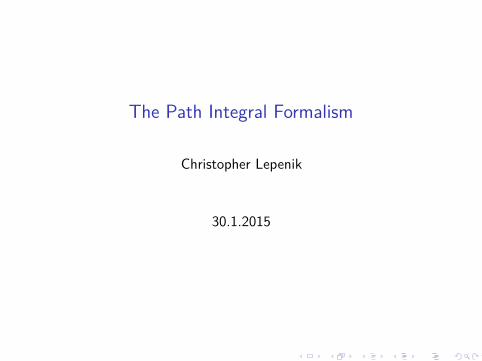
Idea
I Thought Experiment in Quantum Mechanics:I Double slit experiment: MSlit1+Slit2 =MSlit1 +MSlit2I More slits and/or more screens → Addition of all amplitudes
with possible paths through slits.I What happens in the continuum limit of infinitely many screens
and slits? Total amplitude: Sum over all possible paths. →Path Integral.

Introduction Basics Quantization of the Electromagnetic Field The QED Ward-Takahashi Identities
Motivation: Some great Things about the Path Integral inQFT
I No operators, just (anti-)commuting functions.I Very simple quantization.I Useful to quantify non-perturbative effects (e.g. Lattice QCD).I Intrinsic Lorentz invariance due to Lagrangian formalism.I Difficulty of calculation depends on specific problem.I Hard to see that Hamiltonian is positive and hermitian.

Introduction Basics Quantization of the Electromagnetic Field The QED Ward-Takahashi Identities
Path Integrals in Quantum Mechanics - Definition
I Consider transition matrix with 1 d.o.f.:⟨x′, t′ |x, t
⟩=⟨x′∣∣∣exp
(−iH(t′ − t)
)∣∣∣x⟩with xH(t) |x, t〉 = x |x, t〉, xS |x〉 = x |x〉.
I To write down our thought experiment in a mathematical form,we divide time interval (t′ − t) into n+ 1 equal parts of lengthε:
t′ = t+ (n+ 1)ε, tj := t+ jε
Introduction Basics Quantization of the Electromagnetic Field The QED Ward-Takahashi Identities
Path Integrals in Quantum Mechanics - Definition
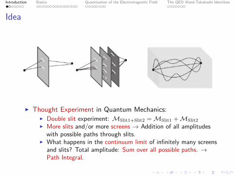
I Using completeness relation∫
dxj |xj , tj〉 〈xj , tj | = 1:
⟨x′, t′ |x, t
⟩=
n∏j=0i=1
∫dxi 〈xj+1, tj+1 |xj , tj 〉
I Using∫ dpj
2π |pj〉 〈pj | = 1 and assuming H = p2
2m + V (x) for ashort-time matrix element:
〈xj , tj |xj−1, tj−1 〉 =⟨xj∣∣exp
(−iεH
)∣∣xj−1⟩
=⟨xj∣∣(1− iεH)∣∣xj−1
⟩+O(ε2)
=∫
dpj2π eipj(xj−xj−1) (1− iεH(pj , xj−1)) +O(ε2)
=∫
dpj2π eipj(xj−xj−1)−iεH(pj ,xj−1) +O(ε2)

Introduction Basics Quantization of the Electromagnetic Field The QED Ward-Takahashi Identities
Path Integrals in Quantum Mechanics - Definition
I Using all that for the full transition matrix element we get
⟨x′, t′
∣∣x, t⟩ = limn→∞
∫ ( n∏j=1
dxj
)∫ (n+1∏j=1
dpj2π
)
× exp
(i
n+1∑j=1
(pj(xj − xj−1)−H(pj , xj−1)ε)
)
= N limn→∞
∫ ( n∏j=1
dxj
)exp
(i
n+1∑j=1
((xj − xj−1)2m
2ε − V (xj−1)))
=: N∫Dx exp
it′∫t
dτ(x2m
2 − V (x))
︸ ︷︷ ︸=L
= N∫Dx exp (iS[x])
I Boundaries: x(t) = x, x(t′) = x′.
I We used∫ dpj
2π exp(i(pj∆x−
εp2j
2m ))
=√
2πmε
exp(
∆x2m2ε
).

Introduction Basics Quantization of the Electromagnetic Field The QED Ward-Takahashi Identities
Path Integrals in field theory
I Generalization to more degrees of freedom.I x(t)→ φ(x, t): D.o.f. labeled by “index” x → infinite d.o.f.I Various mathematical issues in defining the path integral in
field theory (e.g. discrete → continuous).I Much more ambiguous than in quantum mechanics,
nevertheless of great value.

Introduction Basics Quantization of the Electromagnetic Field The QED Ward-Takahashi Identities
Path Integrals in field theory
I Heuristically, the previous derivation can be done also for fields.I Intermediate states much more complicated.I Completeness relation:∫
Dφ |φ〉 〈φ| = 1
I Analogous to quantum mechanics:
⟨φb(~x)
∣∣∣ e−iHT ∣∣∣φa(~x)⟩
= N∫Dφ exp
i T∫0
d4xL
with φ(0, ~x) = φa(~x), φ(T, ~x) = φb(~x).
Introduction Basics Quantization of the Electromagnetic Field The QED Ward-Takahashi Identities
Basics - The Two-Point Function
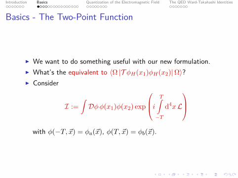
I We want to do something useful with our new formulation.I What’s the equivalent to 〈Ω |T φH(x1)φH(x2)|Ω〉?I Consider
I :=∫Dφφ(x1)φ(x2) exp
i T∫−T
d4xL
with φ(−T, ~x) = φa(~x), φ(T, ~x) = φb(~x).
Introduction Basics Quantization of the Electromagnetic Field The QED Ward-Takahashi Identities
Basics - The Two-Point Function
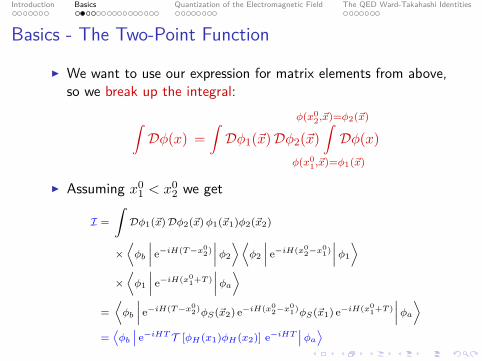
I We want to use our expression for matrix elements from above,so we break up the integral:
∫Dφ(x) =
∫Dφ1(~x)Dφ2(~x)
φ(x02,~x)=φ2(~x)∫
φ(x01,~x)=φ1(~x)
Dφ(x)
I Assuming x01 < x0
2 we get
I =∫Dφ1(~x)Dφ2(~x)φ1(~x1)φ2(~x2)
×⟨φb
∣∣∣ e−iH(T−x02)∣∣∣φ2
⟩⟨φ2
∣∣∣ e−iH(x02−x
01)∣∣∣φ1
⟩×⟨φ1
∣∣∣ e−iH(x01+T )
∣∣∣φa⟩=⟨φb
∣∣∣ e−iH(T−x02)φS(~x2) e−iH(x0
2−x01)φS(~x1) e−iH(x0
1+T )∣∣∣φa⟩
=⟨φb∣∣ e−iHT T [φH(x1)φH(x2)] e−iHT
∣∣φa⟩

Introduction Basics Quantization of the Electromagnetic Field The QED Ward-Takahashi Identities
Basics - The Two-Point Function
I Something we know from particle physics 2! Take limitT →∞(1− iε) to get correlation function.
I Conditions:I ∃ overlap of |φa〉 and |Ω〉,I there is a finite step between the ground energy E0 and the
next energy state.
e−iHT |φa〉 =∑n
e−iEnT |n〉 〈n |φa 〉
T→∞(1−iε)→ e−iE0∞(1−iε) 〈Ω |φa 〉 |Ω〉

Introduction Basics Quantization of the Electromagnetic Field The QED Ward-Takahashi Identities
Basics - The Two-Point Function
I Like in particle physics 2, the overlap factor vanishes, if wenormalize the expression.
I Analogous to the operator formalism, the normalization factorcorresponds to vacuum bubbles.
〈Ω |T φH(x1)φH(x2)|Ω〉 = limT→∞(1−iε)
∫Dφφ(x1)φ(x2) exp
(iT∫−T
d4xL
)∫Dφ exp
(iT∫−T
d4xL
)

Introduction Basics Quantization of the Electromagnetic Field The QED Ward-Takahashi Identities
Basics - The Generating Functional
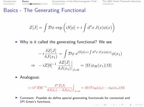
I Generating functional: Great way to calculate correlationfunctions in the p.i. formalism.
I Consider an action in presence of an ext. source J(x). In thiscase J(x) is just an auxiliary field without physical meaning.
I The vacuum amplitude is then the generating functional:
Z[J ] =∫Dφ exp
(iS[φ] + i
∫d4xJ(x)φ(x)
)
Introduction Basics Quantization of the Electromagnetic Field The QED Ward-Takahashi Identities
Basics - The Generating Functional
Z[J ] =∫Dφ exp
(iS[φ] + i
∫d4xJ(x)φ(x)
)
I Why is it called the generating functional? We see
− i δZ[J ]δJ(x1) =
∫Dφ eiS[φ]+i
∫d4x J(x)φ(x)φ(x1)
⇒ − iZ[0]−1 δZ[J ]δJ(x1)
∣∣∣∣J=0
= 〈Ω |φH(x1)|Ω〉
I Analogous:
(−i)nZ[0]−1 δnZ[J ]δJ(x1) · · · δJ(xn)
∣∣∣J=0
= 〈Ω |T φH(x1) · · ·φH(xn)|Ω〉
I Comment: Possible do define special generating functionals for connected and1PI Green’s functions.

Introduction Basics Quantization of the Electromagnetic Field The QED Ward-Takahashi Identities
Example 1 - Free scalar
I Possible to get closed expression for generating functional if weassume that ∃ continuum version of
∞∫−∞
dnx e−i2~xTA~x+i ~J ·~x =
√(−2πi)n
detA ei2~J TA−1 ~J
I Our generating functional
Zfree[J ] =∫Dφ ei
∫d4x (− 1
2φ(x)(+m2−iε)φ(x)+J(x)φ(x))
has this form with A =(+m2 − iε
).
I iε-term needed for convergence. Needed sign corresponds toFeynman-Stuckelberg interpretation without additionalthinking!
I Square root: Canceled by normalization constant.
Introduction Basics Quantization of the Electromagnetic Field The QED Ward-Takahashi Identities
Example 1 - Free scalar
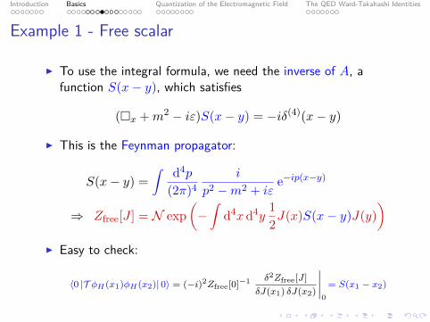
I To use the integral formula, we need the inverse of A, afunction S(x− y), which satisfies
(x +m2 − iε)S(x− y) = −iδ(4)(x− y)
I This is the Feynman propagator:
S(x− y) =∫ d4p
(2π)4i
p2 −m2 + iεe−ip(x−y)
⇒ Zfree[J ] = N exp(−∫
d4x d4y12J(x)S(x− y)J(y)
)I Easy to check:
〈0 |T φH(x1)φH(x2)| 0〉 = (−i)2Zfree[0]−1 δ2Zfree[J ]δJ(x1) δJ(x2)
∣∣∣∣0
= S(x1 − x2)
Introduction Basics Quantization of the Electromagnetic Field The QED Ward-Takahashi Identities
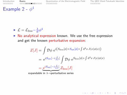
Example 2 - φ4
I L = Lfree− λ4!φ
4
I No analytical expression known. We use the free expressionand get the known perturbative expansion:
Z[J ] =∫Dφ ei(Sfree[φ]+Sint[φ]+
∫d4x J(x)φ(x))
= eiSint[−i δδJ ]∫Dφ eSfree[φ]+
∫d4x J(x)φ(x)
= eiSint[−i δδJ ]︸ ︷︷ ︸expandable in λ→perturbative series
Zfree[J ]
Introduction Basics Quantization of the Electromagnetic Field The QED Ward-Takahashi Identities
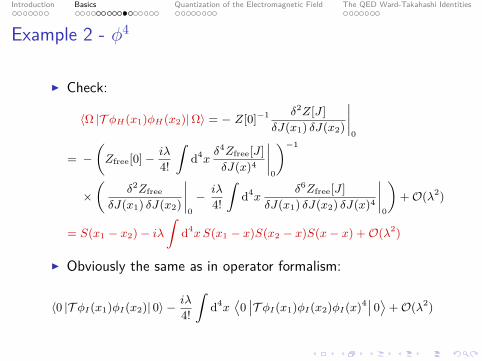
Example 2 - φ4
I Check:
〈Ω |T φH(x1)φH(x2)|Ω〉 = − Z[0]−1 δ2Z[J ]δJ(x1) δJ(x2)
∣∣∣∣0
= −(Zfree[0]− iλ
4!
∫d4x
δ4Zfree[J ]δJ(x)4
∣∣∣∣0
)−1
×(
δ2Zfree
δJ(x1) δJ(x2)
∣∣∣∣0− iλ
4!
∫d4x
δ6Zfree[J ]δJ(x1) δJ(x2) δJ(x)4
∣∣∣∣0
)+O(λ2)
= S(x1 − x2)− iλ∫
d4xS(x1 − x)S(x2 − x)S(x− x) +O(λ2)
I Obviously the same as in operator formalism:
〈0 |T φI(x1)φI(x2)| 0〉 − iλ
4!
∫d4x
⟨0∣∣T φI(x1)φI(x2)φI(x)4∣∣ 0⟩+O(λ2)
Introduction Basics Quantization of the Electromagnetic Field The QED Ward-Takahashi Identities
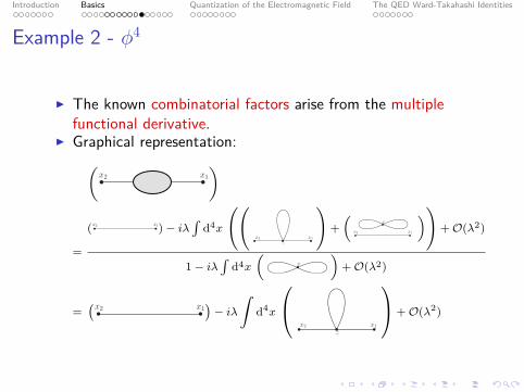
Example 2 - φ4
I The known combinatorial factors arise from the multiplefunctional derivative.
I Graphical representation:(x2 x1
)
=
( x1x2 )− iλ∫
d4x
((x1x2
x
)+(
x1x2
x
))+O(λ2)
1− iλ∫
d4x
(x
)+O(λ2)
=(
x1x2)− iλ
∫d4x
x1x2
x
+O(λ2)
Introduction Basics Quantization of the Electromagnetic Field The QED Ward-Takahashi Identities
Basics - Path Integral for Fermions
I How to quantize fermionic fields?I For x1 6= x2:⟨
Ω∣∣∣T ψH(x1)ψH(x2)
∣∣∣Ω⟩ = −⟨
Ω∣∣∣T ψH(x2)ψH(x1)
∣∣∣Ω⟩I “Classical” Fermi fields must be anticommuting numbers:
These are called “Grassmann numbers”.I For Grassmann variables η and χ:
η, χ = 0 ⇒ η2 = 0⇒ For some function f(η): f(η) = f0 + f1η
I Taylor expansion stops after the linear term.

Introduction Basics Quantization of the Electromagnetic Field The QED Ward-Takahashi Identities
Fermions - Grassmann Numbers
I Definition of left/right derivative:
ddηη = η
←ddη = 1
I Integral over Grassmann variables: Has to maintain shiftinvariance
⇒∫
dη 1 =0 (from shift invariance)∫dη η =1 (normalization)
I Check:∫dη f(η) = f0
∫dη 1+f1
∫dη η η→η+χ= (f0+χf1)
∫dη 1+f1
∫dη η = f1

Introduction Basics Quantization of the Electromagnetic Field The QED Ward-Takahashi Identities
Fermions - Grassmann Numbers
I Remember the important integral∞∫−∞
dnx e−i2~xTA~x+i ~J ·~x =
√(−2πi)n
detA ei2~J TA−1 ~J
I For Grassmann variables:∫dnη dnη ei~η TA~η+i~β·~η+i~η·~β = det(−iA) e−i
~β TA−1~β
I Check in 1 dimension using η → η − a−1β, η → η − βa−1:∫dη dη eiηaη+iβη+iηβ = e−iβa−1β
∫dη dη eiηaη︸ ︷︷ ︸
=1+iηaη
= −ia e−iβa−1β
Introduction Basics Quantization of the Electromagnetic Field The QED Ward-Takahashi Identities
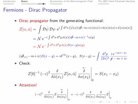
Fermions - Dirac Propagator
I Dirac propagator from the generating functional:
Z[α, α] =∫DψDψ ei
∫d4x (ψ(x)(i∂−m+iε)ψ(x)+α(x)ψ(x)+ψ(x)α(x))
= N e−i∫
d4xd4y α(x)(i∂−m+iε)−1α(y)
= N e−∫
d4xd4y α(x)S(x−y)α(y)
(i∂(x)−m+iε)S(x− y) = iδ(4)(x−y), S(x−y) =∫
d4p
(2π)4i e−ip(x−y)
p−m+ iε
I Check:
Z[0]−1 (−i)2 δ
δα(x1)Z[α, α]←δ
δα(x2)
∣∣∣∣∣∣0
= S(x1 − x2)
I Attention!
(−i)2 δ
δα(x1)Z
←δ
δα(x2)
∣∣∣∣∣0
= −(−i)2 δ
δα(x1)δ
δα(x2)Z
∣∣∣0
Introduction Basics Quantization of the Electromagnetic Field The QED Ward-Takahashi Identities
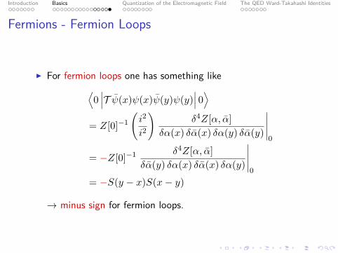
Fermions - Fermion Loops
I For fermion loops one has something like⟨0∣∣∣T ψ(x)ψ(x)ψ(y)ψ(y)
∣∣∣ 0⟩= Z[0]−1
(i2
i2
)δ4Z[α, α]
δα(x) δα(x) δα(y) δα(y)
∣∣∣∣∣0
= −Z[0]−1 δ4Z[α, α]δα(y) δα(x) δα(x) δα(y)
∣∣∣∣∣0
= −S(y − x)S(x− y)
→ minus sign for fermion loops.

Introduction Basics Quantization of the Electromagnetic Field The QED Ward-Takahashi Identities
Quantization of the Electromagnetic Field - Faddeev-Popov
I Consider ∫DA eiS[A]
S[A] =∫
d4x
(−
14
(Fµν)2)
=12
∫d4xAµ(x) (gµν − ∂µ∂ν)Aν(x)
=12
∫d4k
(2π)4 Aµ(k)(−k2gµν + kµkν
)Aν(−k)
I Redundant integration over continuous infinity of physicallyequivalent field configurations due to gauge invariance.
I Very bad: Aµ = kµa is gauge equivalent to 0!I This related to the problem that
(−k2gµν + kµkν)S(γ)νρ (k) = iδµρ
has no solution.
Introduction Basics Quantization of the Electromagnetic Field The QED Ward-Takahashi Identities
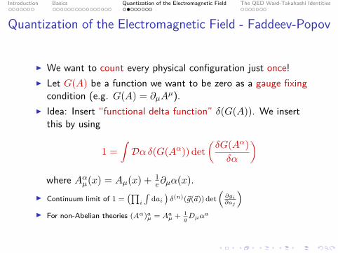
Quantization of the Electromagnetic Field - Faddeev-Popov
I We want to count every physical configuration just once!I Let G(A) be a function we want to be zero as a gauge fixing
condition (e.g. G(A) = ∂µAµ).
I Idea: Insert “functional delta function” δ(G(A)). We insertthis by using
1 =∫Dα δ(G(Aα)) det
(δG(Aα)δα
)where Aαµ(x) = Aµ(x) + 1
e∂µα(x).I Continuum limit of 1 =
(∏i
∫dai)δ(n)(~g(~a)) det
(∂gi∂aj
)I For non-Abelian theories (Aα)aµ = Aaµ + 1
gDµαa
Introduction Basics Quantization of the Electromagnetic Field The QED Ward-Takahashi Identities
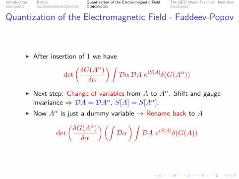
Quantization of the Electromagnetic Field - Faddeev-Popov
I After insertion of 1 we have
det(δG(Aα)δα
)∫DαDA eiS[A]δ(G(Aα))
I Next step: Change of variables from A to Aα. Shift and gaugeinvariance ⇒ DA = DAα, S[A] = S[Aα].
I Now Aα is just a dummy variable → Rename back to A
det(δG(Aα)δα
)(∫Dα
)∫DA eiS[A]δ(G(A))

Introduction Basics Quantization of the Electromagnetic Field The QED Ward-Takahashi Identities
Quantization of the Electromagnetic Field - Faddeev-Popov
det(δG(Aα)δα
)(∫Dα
)∫DA eiS[A]δ(G(A))
I Specify gauge-fixing function G(A): G(A) = ∂µAµ(x)− ω(x)⇒ det
(δGδα
)= det
(e
), independent of any field → can be
treated as normalization constant.
det(e
)(∫Dα
)∫DA eiS[A]δ(∂µAµ − ω(x))
I This is not valid in a non-Abelian gauge theory, becausedet
(∂µDµ
g
)is not field independent.
Introduction Basics Quantization of the Electromagnetic Field The QED Ward-Takahashi Identities
Quantization of the Electromagnetic Field - Faddeev-Popov
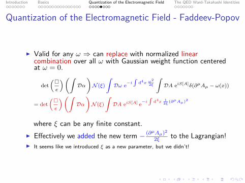
I Valid for any ω ⇒ can replace with normalized linearcombination over all ω with Gaussian weight function centeredat ω = 0.
det(
e
)(∫Dα)N (ξ)
∫Dω e−i
∫d4x ω
22ξ
∫DA eiS[A]δ(∂µAµ − ω(x))
= det(
e
)(∫Dα)N (ξ)
∫DA eiS[A] e−i
∫d4x 1
2ξ (∂µAµ)2
where ξ can be any finite constant.I Effectively we added the new term − (∂µAµ)2
2ξ to the Lagrangian!I It seems like we introduced ξ as a new parameter, but we didn’t!

Introduction Basics Quantization of the Electromagnetic Field The QED Ward-Takahashi Identities
Quantization of the Electromagnetic Field - Faddeev-Popov
I Is it now possible to derive the photon propagator? We definethe generating functional∫
DA e∫
d4x(i2Aµ(x)(gµν−∂µ∂ν)Aν(x)− i
2ξ (∂µAµ)2+JµAµ)
=∫DA ei
∫d4x(
12Aµ(x)
(gµν−∂µ∂ν
(1− 1
ξ
))Aν(x)+JµAµ
)= N e−
i2
∫d4x d4y Jµ(x)
(gµν−∂µ∂ν
(1− 1
ξ
))−1Jν(y)
I In momentum space wee need to solve(−k2gµν +
(1− 1
ξ
)kµkν
)Sνρ(γ)(k) = iδρµ
⇒ Sνρ(γ)(k) = −ik2 + iε
(gνρ − (1− ξ)k
νkρ
k2
).

Introduction Basics Quantization of the Electromagnetic Field The QED Ward-Takahashi Identities
Quantization of the Electromagnetic Field - Faddeev-Popov
I Correlation functions N∫DAO(A) eiS[A] of gauge invariant
operators O(A) is clearly independent of ξ.I In practice: Insert specific value for ξ. Popular choices:
I Feynman gauge: ξ = 1,I Landau gauge: ξ = 0.
Introduction Basics Quantization of the Electromagnetic Field The QED Ward-Takahashi Identities
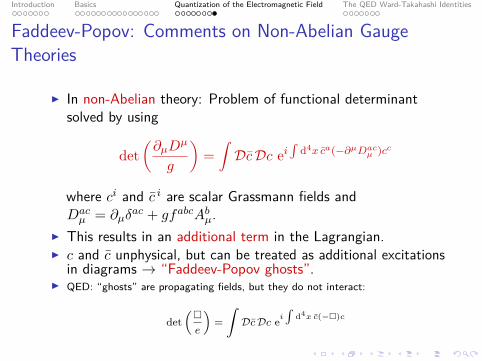
Faddeev-Popov: Comments on Non-Abelian GaugeTheories
I In non-Abelian theory: Problem of functional determinantsolved by using
det(∂µD
µ
g
)=∫DcDc ei
∫d4x ca(−∂µDacµ )cc
where ci and c i are scalar Grassmann fields andDacµ = ∂µδ
ac + gfabcAbµ.I This results in an additional term in the Lagrangian.I c and c unphysical, but can be treated as additional excitations
in diagrams → “Faddeev-Popov ghosts”.I QED: “ghosts” are propagating fields, but they do not interact:
det(
e
)=∫DcDc ei
∫d4x c(−)c
Introduction Basics Quantization of the Electromagnetic Field The QED Ward-Takahashi Identities
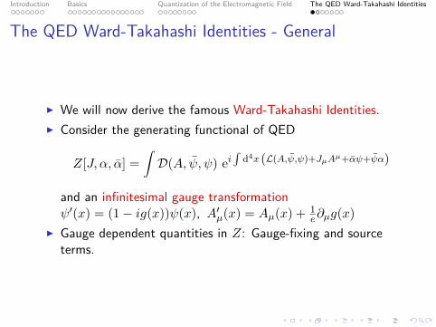
The QED Ward-Takahashi Identities - General
I We will now derive the famous Ward-Takahashi Identities.I Consider the generating functional of QED
Z[J, α, α] =∫D(A, ψ, ψ) ei
∫d4x (L(A,ψ,ψ)+JµAµ+αψ+ψα)
and an infinitesimal gauge transformationψ′(x) = (1− ig(x))ψ(x), A′µ(x) = Aµ(x) + 1
e∂µg(x)I Gauge dependent quantities in Z: Gauge-fixing and source
terms.

Introduction Basics Quantization of the Electromagnetic Field The QED Ward-Takahashi Identities
The QED Ward-Takahashi Identities - General
I After applying the transformation, we expand in g(x) up toO(g):∫
d4x
∫D(A, ψ, ψ) ei(S[A,ψ,ψ]+Source)
×(
1− g(x)(−
1e∂µJ
µ(x)− iα(x)ψ(x) + iψ(x)α(x)−1e∂µµνAν(x)
))with µν = gµν −
(1− 1
ξ
)∂µ∂ν .
I We get rid of the 1 by subtracting the original expression(→ δZ). We now arrive at the Ward-Takahashi Identity:
0 =δZ
δg(y)
∣∣∣g=0
=1e∂µ(y)Jµ(y)Z + iα(y)
δZ
δα(y)+ i
δZ
δα(y)α(y) +
1e∂
(y)µ
µν(y)
δZ
δJν(y)
Introduction Basics Quantization of the Electromagnetic Field The QED Ward-Takahashi Identities
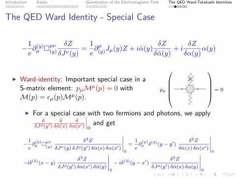
The QED Ward Identity - Special Case
−1e∂(y)µ
µν(y)
δZ
δJν(y) = 1e∂µ(y)Jµ(y)Z + iα(y) δZ
δα(y) + iδZ
δα(y)α(y)
I Ward-identity: Important special case in aS-matrix element: pµMµ(p) = 0 withM(p) = εµ(p)Mµ(p).
pµ
µ
↓p
= 0
I For a special case with two fermions and photons, we applyδ
δJρ(y′)δ
δα(x)δ
δα(x′)
∣∣∣0
and get
−1e∂
(y)µ
µν(y)
δ4Z
δJν(y) δJρ(y′) δα(x) δα(x′)
∣∣∣∣0
=1e∂
(y)ρ δ(4)(y − y′)
δ2Z
δα(x) δα(x′)
∣∣∣∣0
−iδ(4)(x− y)δ3Z
δJρ(y′) δα(x′) δα(y)
∣∣∣∣0
− iδ(4)(y − x′)δ3Z
δJρ(y′) δα(x) δα(y)
∣∣∣∣0
Introduction Basics Quantization of the Electromagnetic Field The QED Ward-Takahashi Identities
The QED Ward Identity - Special Case
∂(y)µ
µν(y)
ν
y
y′
x′x
ρ
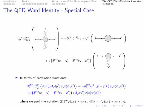
= −∂(y)ρ δ(4)(y − y′)
(x′x
)
+ e(δ(4)(x− y)− δ(4)(y − x′)
)y′
x′x
ρ
I In terms of correlation functions:
∂(y)µ
µν(y)
⟨Aν(y)Aρ(y′)ψ(x)ψ(x′)
⟩= −∂(y)
ρ δ(4)(y − y′)⟨ψ(x)ψ(x′)
⟩+e(δ(4)(x− y)− δ(4)(y − x′)
) ⟨Aρ(y′)ψ(x)ψ(x′)
⟩where we used the notation 〈Ω |T ϕ(x1) · · ·ϕ(xn)|Ω〉 =: 〈ϕ(x1) · · ·ϕ(xn)〉.
Introduction Basics Quantization of the Electromagnetic Field The QED Ward-Takahashi Identities
The QED Ward Identity - Special Case
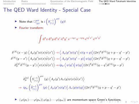
I Note that µν(y) is i(S−1
(γ)
)µν(y)!
I Fourier transform:∫d4xd4y d4x′ d4y′ e−iqx e−ipy eiq
′x′ eip′y′
δ(4)(x− y)⟨Aρ(y′)ψ(x)ψ(x′)
⟩→⟨Aρ(p′)ψ(q′)
∣∣ψ(q + p)⟩(2π)4δ(4)(q + p− q′ − p′)
δ(4)(y − x′)⟨Aρ(y′)ψ(x)ψ(x′)
⟩→⟨Aρ(p′)ψ(q′ − p)
∣∣ψ(q)⟩(2π)4δ(4)(q + p− q′ − p′)
∂(y)ρ δ(4)(y − y′)
⟨ψ(x)ψ(x′)
⟩→ ipρ
⟨ψ(q′)
∣∣ψ(q)⟩
(2π)8δ(4)(q − q′)δ(4)(p− p′)
∂(y)µ
(S−1
(γ)
)µν(y)⟨Aρ(y′)Aν(y)ψ(x)ψ(x′)
⟩→ ipµ
(S−1
(γ)
)µν(p)⟨Aρ(p′)ψ(q′)
∣∣Aν(p)ψ(q)⟩(2π)4δ(4)(q + p− q′ − p′)
I 〈ϕ(p1) · · ·ϕ(pn)|ϕ(q1) · · ·ϕ(qm)〉 are momentum space Green’s functions.
Introduction Basics Quantization of the Electromagnetic Field The QED Ward-Takahashi Identities
The QED Ward Identity - Special Case
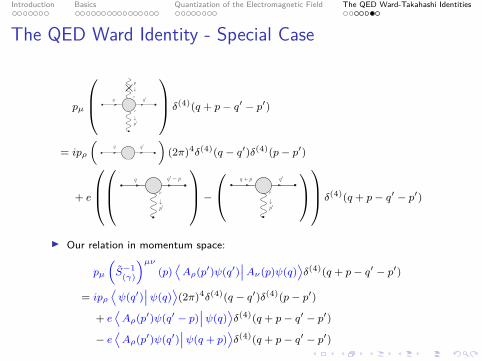
pµ
ν
ρ
q
↓p
↓p′
q′
δ(4)(q + p− q′ − p′)
= ipρ
(q′q
)(2π)4δ(4)(q − q′)δ(4)(p− p′)
+ e
ρ
q
↓p′
q′ − p
− ρ
q + p
↓p′
q′ δ(4)(q + p− q′ − p′)
I Our relation in momentum space:
pµ
(S−1
(γ)
)µν(p)⟨Aρ(p′)ψ(q′)
∣∣Aν(p)ψ(q)⟩δ(4)(q + p− q′ − p′)
= ipρ⟨ψ(q′)
∣∣ψ(q)⟩(2π)4δ(4)(q − q′)δ(4)(p− p′)
+ e⟨Aρ(p′)ψ(q′ − p)
∣∣ψ(q)⟩δ(4)(q + p− q′ − p′)
− e⟨Aρ(p′)ψ(q′)
∣∣ψ(q + p)⟩δ(4)(q + p− q′ − p′)
Introduction Basics Quantization of the Electromagnetic Field The QED Ward-Takahashi Identities
The QED Ward Identity - Special Case
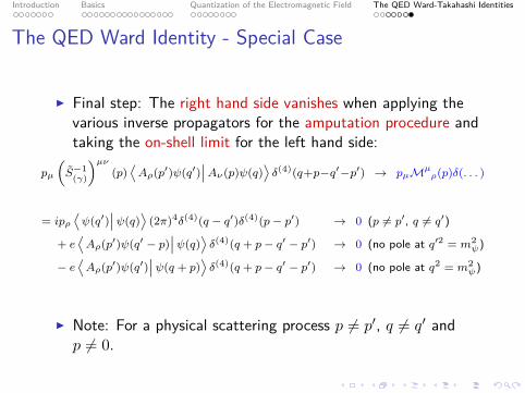
I Final step: The right hand side vanishes when applying thevarious inverse propagators for the amputation procedure andtaking the on-shell limit for the left hand side:
pµ
(S−1
(γ)
)µν(p)⟨Aρ(p′)ψ(q′)
∣∣Aν(p)ψ(q)⟩δ(4)(q+p−q′−p′) → pµMµ
ρ(p)δ(. . . )
= ipρ⟨ψ(q′)
∣∣ψ(q)⟩
(2π)4δ(4)(q − q′)δ(4)(p− p′) → 0 (p 6= p′, q 6= q′)
+ e⟨Aρ(p′)ψ(q′ − p)
∣∣ψ(q)⟩δ(4)(q + p− q′ − p′) → 0 (no pole at q′2 = m2
ψ)
− e⟨Aρ(p′)ψ(q′)
∣∣ψ(q + p)⟩δ(4)(q + p− q′ − p′) → 0 (no pole at q2 = m2
ψ)
I Note: For a physical scattering process p 6= p′, q 6= q′ andp 6= 0.

Introduction Basics Quantization of the Electromagnetic Field The QED Ward-Takahashi Identities
Conclusions
I Different approach to quantum theory.I Explicit Lorentz Symmetry.I Depending on problem, much easier or much more difficult
calculation than in operator formalism.I Easy to derive Feynman rules directly from the Lagrangian.I Easy derivation of the Ward-identity from gauge symmetry.I Essential for quantizing gauge theories (especially non-Abelian).
Introduction Basics Quantization of the Electromagnetic Field The QED Ward-Takahashi Identities
References
I M. D. Schwartz: Quantum Field Theory and the StandardModel. Cambridge University Press, Cambridge (2014)
I S. Pokorski: Gauge Field Theories, Second Edition. CambridgeUniversity Press, Cambridge (2000)
I M. E. Peskin, D. V. Schroeder: An Introduction to QuantumField Theory. Perseus Books, New York (1995)