Colorado State

University

DEPARTMENT OF ATMOSPHERIC SCIENCE

Paper No. 770

The Partnership of Weather and Air Quality

An Essay

Roger A. Pielke Sr.

April 20, 2006

The Partnership of Weather and Air Quality

An Essay

Roger A. Pielke Sr.

University of Colorado, CIRES

Boulder, CO 80309

and

Colorado State University

Department of Atmospheric Science

Fort Collins, CO 80523

pielke@cires.colorado.edu

April 20, 2006

Atmospheric Science Paper No. 770

2

Abstract

As part of the celebration of the Golden Jubilee of the EPA/NOAA partnership, this

paper provides a perspective on the movement towards a merger of the disciplines of weather

and air quality science. Also presented are several major conclusions regarding the modeling of

atmospheric dispersion, which have resulted in the use of combined knowledge from both

disciplines These conclusions include the recognition that dispersion is greater than evaluated

from Gaussian models in situations with significant large scale wind flow over heterogeneous

landscapes, but overestimated in light wind conditions, particularly in heterogeneous landscapes.

Methodologies are proposed that would improve the ability to model the interactions of

weather and air quality. These include the replacement of existing parameterizations with much

more computationally efficient look-up-tables, the calculation of the linear and nonlinear

components of the models separately, and use of wind tunnel modeling to improve the accuracy

of the numerical models.

3

1. Introduction

The scientific communities of weather and air quality have developed out of different

disciplines. Weather, involving, for example, temperature, precipitation and cloud cover, has

utilized meteorologists for both research and operations, while air quality developed out of the

atmospheric chemistry community. Climate, as shown below, has developed two, contradictory

definitions, as the merger of the disciplines of weather and air quality has erratically progressed.

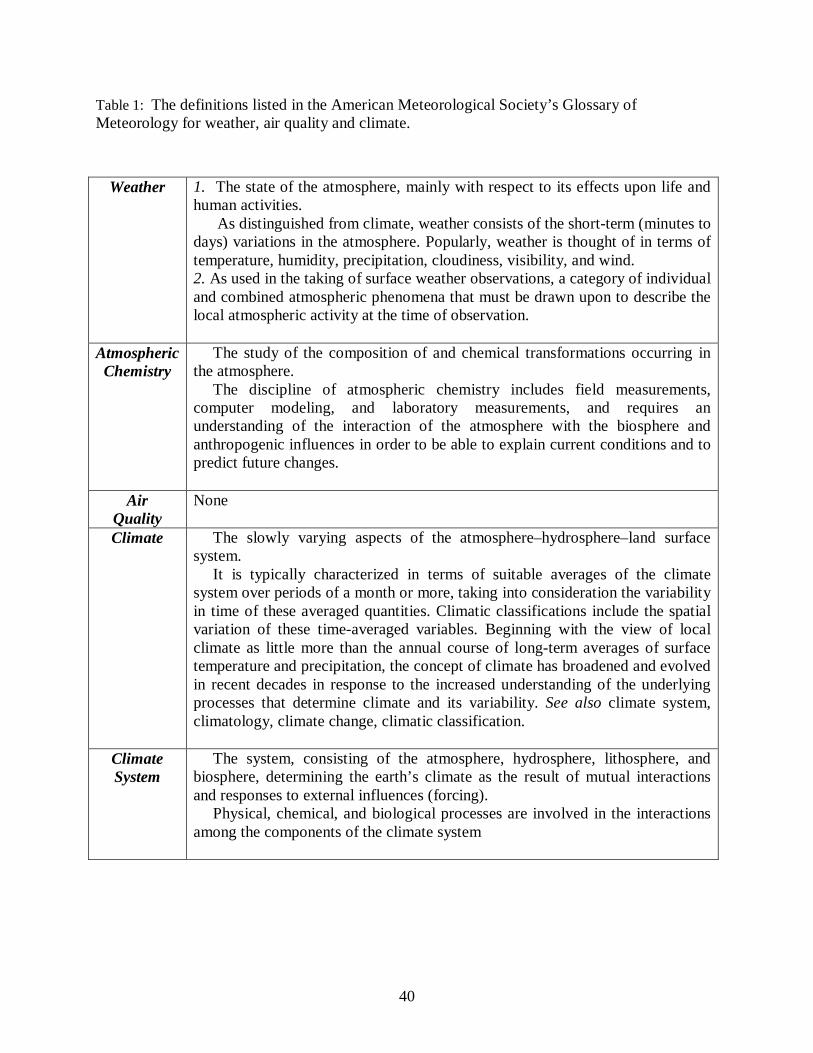
Table 1 illustrates the definitions listed in the American Meteorological Society’s

Glossary of Meteorology for weather, air quality, and climate. This Glossary, unfortunately,

shows that the partnership of weather and air quality still has quite a way to go. “Air Quality” is

not even defined! “Climate” is defined more narrowly than “climate system”. With “climate”,

while the definition has started to move to a more inclusive framework (such as illustrated in Fig.

1), the Glossary still focuses on “suitable averages of the climate system over periods of a month

or more.” The reality is the “climate system” is a synonym for “climate”. The term “climate”,

should also explicitly include “weather” and “air quality” as integral components.

This paper provides an illustration as to why the partnership of weather and air quality is

essential if we are to advance our understanding of climate. The recognition of this need, and

movement to develop this interaction, has been one of the major achievements of the

EPA/NOAA Partnership.

2. Examples of What We Have Learned Over the Last 50 Years

There are several terms that have become accepted over the last several decades that

demonstrate movement toward the integration of weather and air quality, in this case with

4

respect to atmospheric turbulent processes. These terms are given in Table 2. In the early years

of air quality studies (and as still perpetuated today), dispersion has been estimated with

Gaussian plume and puff models (e.g., Turner 1969). While a seminal contribution at the time,

there are serious shortcomings, however, that have resulted from limiting dispersion to Gaussian

behavior (see also Zannetti 1990 and Pielke 1984, Chapter 7 for discussions on the limitations of

this assumption with respect to dispersion). The NRC (2003) entitled “Managing Carbon

Monoxide Pollution in Meteorological and Topographical Problem Areas” illustrates why a

broader view of dispersion is required, and why the Gaussian format is inadequate to skillfully

characterize the combination of air quality and weather processes.

This section provides evidence of the limitations of the Gaussian model approach for two

different situations.

a. Gaussian Puff and Plume Models Underestimate Dispersion with Significant Large-Scale Winds with Landscape Heterogeneities

Even in flat terrain, Gaussian models have serious inadequacies. To show this, a two-

dimensional boundary layer model, as reported in Pielke and Uliasz (1993), was integrated with

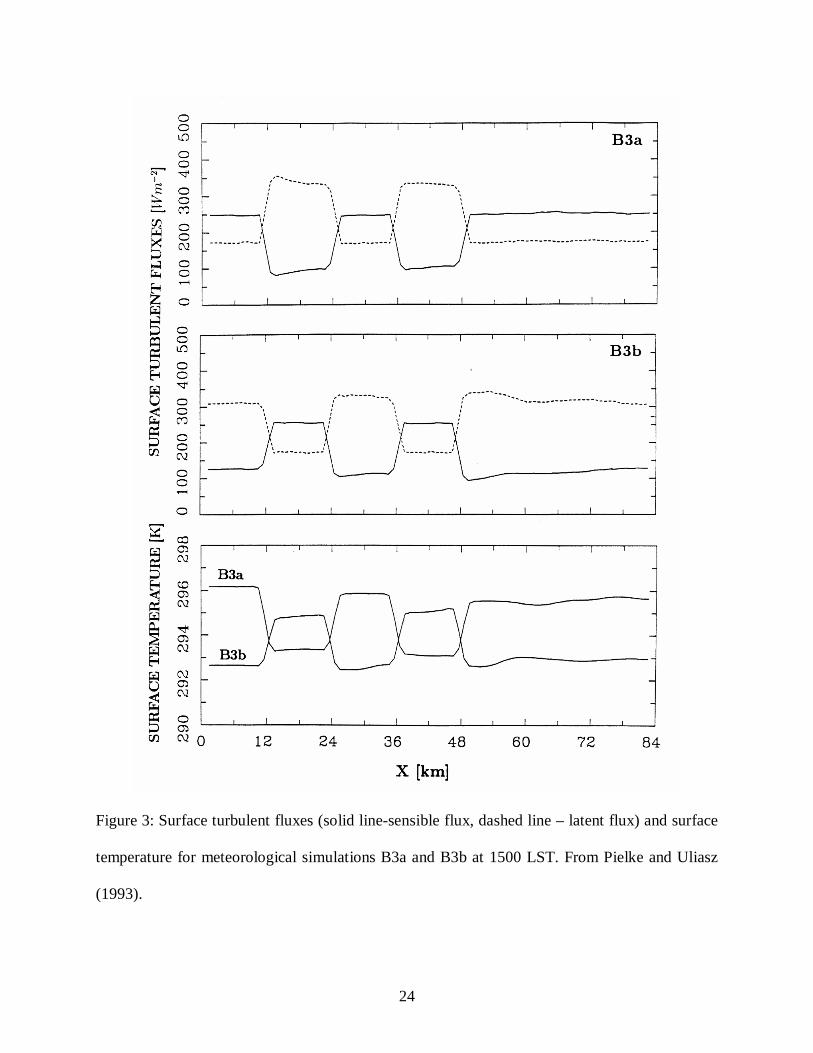
the small spatial-scale landscape patchiness shown in Fig. 2. An illustration of two of the spatial

patterns of heat fluxes and surface temperature for these landscape patches is given in Fig. 3.

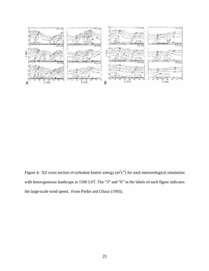
Figure 4 presents a snapshot of the simulated turbulent kinetic energy for each of the landscape

patch distributions for relatively light large-scale winds (3 m s-1).

Figure 5 shows the dispersion from a point source for this relatively light large-scale

wind (3 m s-1). The top left figure is closest to a Gaussian plume distribution, but even here,

where there is no landscape patchiness, the turning of winds with height in the planetary

boundary layer results in spread of the lowest effluent to the right of the plume. With the stronger

5

large-scale winds (6 m s-1), the spread at lower levels is still evident in each of the simulations

for different patchiness, but the plume behavior is closer to a Gaussian plume distribution even

when landscape patches of the size prescribed in these simulations are present (Fig. 6).

The surface distribution of concentrations at different downwind distance, assuming a

passive pollutant on this time scale (such as CO), is shown in Fig. 7. The obvious deviation from

a Gaussian plume distribution is evident in each the plots, even those that visually appear closer

to being Gaussian in Figures 5 and 6 Table 3 further summarizes the differences in a tabular

form for different simulation cases. Since the real world also has other heterogeneities (such a

time-varying large-scale winds), this set of idealized experiments shows the inaccuracies that are

inevitable if a Gaussian plume model is used.

The conclusions are:

• Dispersion is enhanced over heterogeneous landscapes as contrasted with the same flow

over a homogeneous landscape.

• The importance of the heterogeneity becomes less as the wind speed increases and/or the

spatial scale of the heterogeneity becomes smaller.

• The use of standard Gaussian plume or puff models in heterogeneous landscapes will

lead to erroneous estimates of concentrations.

b. Gaussian Puff and Plume Models Overestimate Dispersion with Light Large-Scale Winds in Heterogeneous Landscapes

Light large-scale winds are common when polar high pressure systems overlie a region.

Figure 8, from Pielke et al. (1991), provides examples of weather patterns which produce such

light winds (Category 4 in the Figure). In locations with topographic terrain, such large-scale

6

light winds results in weather that is dominated by mesoscale and smaller wind circulations. The

weather patterns can be cataloged into regions of higher and lower dispersion (Fig. 9).

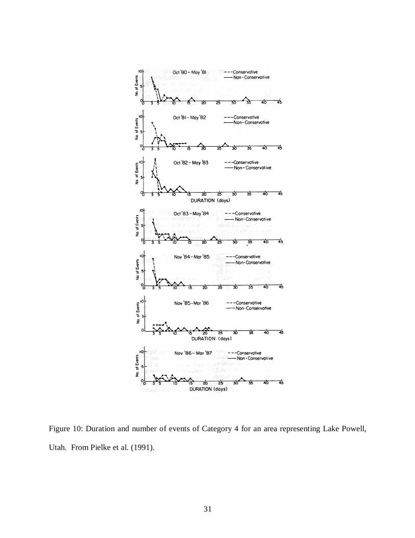
These synoptic categories can be used to determine the persistence of reduced dispersion.

As an example, Fig. 10 shows the duration and number of events of polar high light large-scale

wind conditions for Lake Powell, Arizona over 6 years. These events of limited dispersion (and

thus a potential case for air quality to deteriorate) lasted in one case at least as long as 23 days,

even using a conservative definition of the polar high category.

Pollution buildups over time can be quite large under these light wind synoptic situations.

As summarized and quoted from Pielke et al. (1991);

“Despite the lack of attention by the regulatory agencies to trapping valleys, a very

simple algorithm can be used to estimate potential or actual pollution impacts due to local

sources within such a valley. This algorithm cam be expressed as

/( )C E t x y z= ∆ ∆ ∆ (1)

where x y z∆ ∆ ∆ is the volume into which pollution is at a rate of E over a time period t and C is

the concentration of the pollution (i.e., mass per unit volume). The dimensions x∆ and y∆ could

correspond to the horizontal dimensions of a valley, or to that portion of the valley over which

the pollution spreads, while z∆ would be the layer in the atmosphere into which the pollution is

ejected. In a daytime, well-mixed boundary layer, this layer would correspond to the distance

from the surface to the inversion height, whereas in a stable, stratified pool of cold air, this

would correspond to some fraction of the inversion height. The time, t, would correspond to the

length of time (i.e., persistence) of the trapped circulation, while E is the input of pollution above

some baseline (which could be zero). C represents the maximum uniformly distributed

concentration of an elemental chemical (e.g., sulfur, carbon) over the volume x y z∆ ∆ ∆ since

7

deposition to the surface is ignored. While this conceptually simple model needs to be validated,

it is a plausible approach to represent pollution build-up in trapping valleys.

In order to illustrate the use of Eq. (1) to assess air quality impacts for a valley which

acts to some extent as a trapping valley, the possible effects of a source in the Grand Valley of

Colorado near Grand Junction on Colorado National Monument will be assessed for a typical

wintertime stagnation event. The variables in Eq. (1) are defined as

(2 km) 1iz zβ β β∆ = = ≤

20kmy∆ =

x yα∆ = ∆ (2)

9dayst =

125g s of SE −=

where the sulfur is primarily in the form of SO2.

In Eq. (2), β represents the fraction of the inversion height into which the pollution is

input and diffused. The inversion height is estimated from the climatological analyses of Hanson

and McKee (1983), and is below the elevation of the valley sides. The distance y∆ is the

approximate width of the valley, while α represents the distance of pollution dispersal along the

valley with respect to the valley width. The time, t, of an episode is selected as nine days based

on the information discussed in Section 2. E is a realistic estimate of SO2 input from a relatively

small industrial facility. Using these values, Ea. (1) can be rewritten as

( )5

3 (2.43 10 )g mC

αβ

−− ×

= (3)

The 24-h primary air quality standard for SO2 at a Class I air quality area in the United

States is expected to be the most sensitive to violation as a result of a nine-day stagnation event.

8

The 24-h standard is 5 ×10-6 g m-3. Thus Eq. (3) indicates a violation if the volume covered by

x y z∆ ∆ ∆ includes a Class I area and 5αβ < .

Colorado National Monument has been categorized as a State of Colorado equivalent to

a Federal class I area for SO2. The state nomenclature refers to it as a Category I area. Thus

depending on the values of α and β . In a stable layer of pooled air, it is expected thatβ

would be on the order of 10% of the inversion height since a surface non-buoyant emission

would tend to be confined close to the ground while on elevated release would stabilize around

the effective stack height (as long as the effective stack height remains below the inversion). The

along valley direction for the example is more difficult to estimate, however, but a distance of

200 km( 10)α = is likely to represent the largest horizontal area covered.”

Even in flat terrain, pollution can accumulate over time if the winds are light such that

mesoscale circulations develop. In Section 2a it is shown that dispersion is enhanced when large-

scale winds blow over small-scale spatial landscape heterogeneities. Here we show that larger-

scale landscape heterogeneities which generate mesoscale circulations can reduce dispersion as

air recirculates within the mesoscale circulation.

Eastman et al. (1995) ran a series of mesoscale model simulations to assess the role of

Lake Michigan in altering dispersion patterns. Figure 11 presents the set of model simulations,

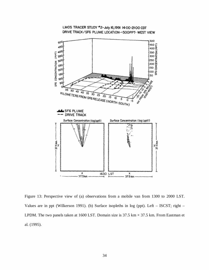
while Fig. 12 shows the resultant dispersion patterns. Only the figure in the lower right of Fig. 13

is close to a Gaussian plume, which occurs without the Lake or any landscape heterogeneity.

Figure 13 compares observed surface concentrations of a passive tracer released during a field

campaign with the mesoscale model which includes the Lake, and a Gaussian plume estimate of

the dispersion. The mesoscale model results are clearly more accurate. Table 4 shows that there

9

is a recirculation of pollutants such that air quality degrades as the pollutants accumulate. With

the simulation of no lake, there is no recirculation.

The conclusions, exemplified by these examples, are:

• Inability of Gaussian puff and plume models to include recirculation.

• Under light large-scale flow, dispersion estimates from Gaussian puff and plume models

overestimate dispersion in heterogeneous terrain.

3. Climate is becoming an Integrator of Weather and Air Quality The climate community has been seeking to force a focus on climate that is based on a

top-of-the-atmosphere, globally-averaged radiative forcing (e.g., see Fig. 14). While atmospheric

chemistry has entered the discussion (see the 2005 National Research Council (NRC) report

http://www.nap.edu/books/0309095069/html/31.html), there is increasing recognition on the

complex role of weather and air chemistry interactions, as illustrated by the summary of aerosol

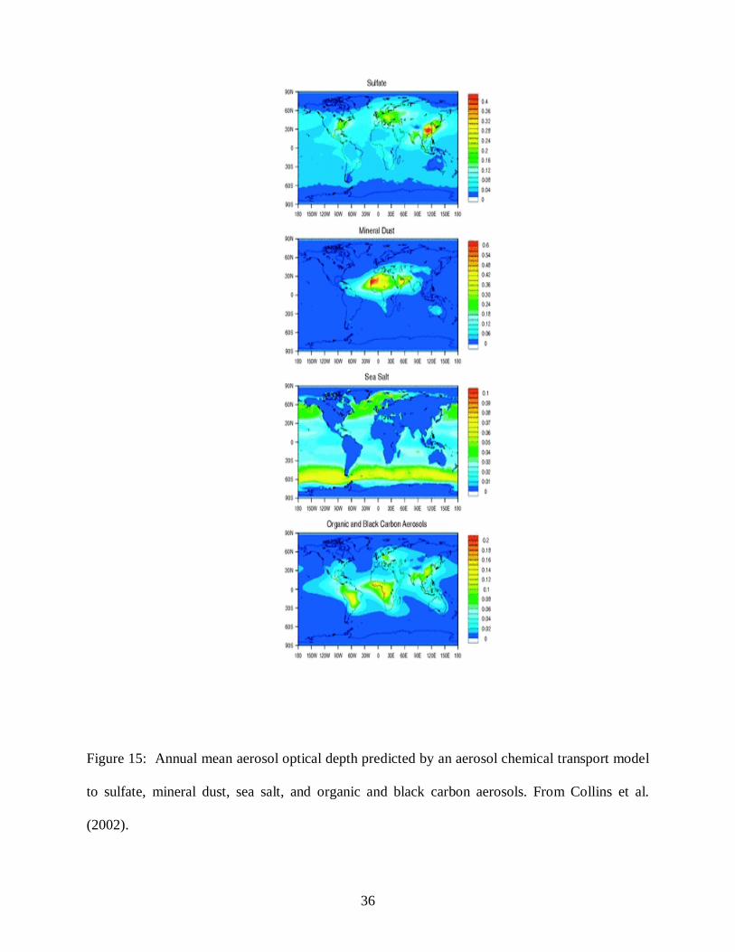
indirect forcings listed in Table 5. The spatial pattern distribution of aerosol forcings (see Fig.

15) shows that their climate forcing requires a regional characterization of weather in order to

understand these interactions.

Indeed, the summary of the aerosol direct climate forcing from the 2005 NRC report

documents this merger of weather and air quality, i.e.,

“The average global mean aerosol direct forcing from fossil fuel combustion and

biomass burning is in the range from −0.2 to −2.0 W m−2 (IPCC 2001). This large range

results from uncertainties in aerosol sources, composition, and properties used in

different models. Recent advances in modeling and measurements have provided

10

important constraints on the direct effect of aerosols on radiation (Ramanathan et al.,

2001a; Russell et al., 1999; Conant et al., 2003). Critical gaps, discussed further below,

relate to spatial heterogeneity of the aerosol distribution, which results from the short

lifetime (a few days to a week) against wet deposition; chemical composition, especially

the organic fraction; mixing state and behavior (hygroscopicity, density, reactivity, and

acidity); and optical properties associated with mixing and morphology (refractive index,

shape, solid inclusions). The chemical composition of particles is in general not well

known.”

4. What Needs to be Accomplished to Further Promote the Integration of Weather and Air Quality Science

There are five model concepts that provide opportunity areas for future research if we are

to improve the integration of weather and air quality science. These are:

• The only basic physics in atmospheric models are advection, gravity and the pressure

gradient force.

• All other components of the models are parameterized as column or box modules using

tunable coefficients and functions.

• The tuning is completed for idealized situations (i.e., “golden days”).

• There is a mismatch between the model grid volume and the observed volume of

measurement.

• There is a mismatch between the atmospheric model grid volume and what is required for

accurate reactive chemistry.

11

Figure 16 shows that all parameterizations in weather and air quality models are column (1-D) or

box representations. Therefore these types of models are engineering code, and not basic physics

or chemistry codes. Hence there is an opportunity to improve the skill of these parameterizations.

The engineering character of the parameterizations can be shown with the following text

reproduced from Pielke (2002);

“It is useful to dissect a parameterization algorithm to determine the number of

dependent variables and, adjustable and universal parameters that are introduced. This

dissection can be illustrated with the following simple example. Holtslag and Boville (1993) and

Tijm et al. (1999a) propose the following form for Kθ above the boundary layer:

2 (Ri),K l S Fθ θ θ= (4)

1 1 1

l kzθ θλ= = (5)

,V

Sz

∂=∂

�

(6)

and

1/2(1-18Ri) Ri 0(Ri)=

2) 1/(1+10 Ri+80 Ri Ri 0.Fθ

≤

> (7)

{300 m, 1km30 m= 270 exp (1 ( /1000 m)),

zzθλ

≤=−

(8)

This formulation of Kθ includes the following dependent variables, parameters, and prescribed

constants:

• In Eq. (4), the dependent variables lθ, S, and Fθ define Kθ.

12

• In Eq. (5), lθ is defined with the independent variable z, the dependent variable λθ, and

the parameter k.

• In Eq. (6), S is defined by the vertical gradient of V�

.

• In Eq. (7), Fθ (Ri) is defined by the dependent variable Ri [the gradient Richardson

number which is proportional to the ratio of the S to the vertical temperature gradient)],

and the constants 18, 10, and 80, and the exponent 1/2.

• In Eq. (8), λθ is defined by the independent variable z, and the constants 300, 30, 270,

and 1000.

Therefore, to represent the term Kθ, in addition to the fundamental variables iu and θ , one

parameter (k) and 8 constants (18, 10, 80, 1/2, 300, 30, 270, 1000) must be provided.”

The data to tune these parameterizations are also based on what are referred to as “golden

days”. Day 33-34 of the Wangara Experiment is one example of data that has been used to tune

boundary layer models (a google search shows the many papers on this particular day of an

observational field campaign

http://scholar.google.com/scholar?hl=en&lr=&q=Day+33+Wangara&btnG=Search). The tuned

parameterization is then used for all days, not just days that conform to the conditions of the

“golden days”! This approach is applied to all of the parameterizations.

The model also uses grid-volume averages to define the variables used (Fig. 17), while

the observations are point, line, and only occasionally volume averages (the later from remote

sensing platforms such as lidars). The spread between the selected parameterization and the

observations can be significant (see Fig. 18), yet this uncertainly has almost always been

ignored.

13

The recommendations to improve weather and air quality models and their integration

include the following:

1. Use a look-up table approach to increase parameterization efficiency as proposed

in Pielke et al. (2006). An improvement in efficiency by a factor of ten or more is

anticipated.

2. Decompose the models into linear and nonlinear components and compute the

former analytically. Only the nonlinear part needs to be computed numerically.

This will increase the accuracy of the models since numerical errors will be

reduced (Leoncini and Pielke 2005; Weidman and Pielke 1983).

3. Insert uncertainty associated with the parameterizations into the model

calculations, such that a spread of simulation realizations is achieved. This is a

type of ensemble prediction. (Garratt et al. 1990).

4. Use wind tunnel modeling to develop more accurate parameterizations for the

spatial and temporal scales where the solution spaces accurately overlap as shown

in Avissar et al. 1990.

5. Conclusions

The weather and air quality communities have come closer together. However, there is

still considerable work to do to make it a real merger. Modeling opportunities exist to improve

our skill at understanding air pollution issues on all time and space scales, and to better assess the

predictability of the consequences of weather and air quality interactions.

14

Acknowledgements

The AMS is thanked for providing the support to attend and present at the AMS/EPA

Golden Jubilee in Durham, North Carolina. Research support to complete this paper was

provided by NASA Grant No. NNG04GB87G.

15

REFERENCES

Avissar, R., M.D. Moran, R.A. Pielke, G. Wu, and R.N. Meroney, 1990: Operating ranges of

mesoscale numerical models and meteorological wind tunnels for the simulation of sea

and land breezes. Bound.-Layer Meteor., Special Anniversary Issue, Golden Jubilee, 50,

227-275.

Conant, W.C., J.H. Seinfeld, J. Wang, G.R. Carmichael, Y. Tang, I. Uno, P.J. Flatau, K.M.

Markowicz, and P.K. Quinn. 2003: A model for the radiative forcing during ACE-Asia

derived from CIRPAS Twin Otter and R/V Ronald H. Brown data and comparison with

observations. J. Geophys. Res., 108(D23), 8661, DOI: 10.1029/ 2002JD003260.

Eastman, J.L. R.A. Pielke, and W.A. Lyons, 1995: Comparison of lake-breeze model simulations

with tracer data. J. Appl. Meteor., 34, 1398-1418.

Garratt, J.R., R.A. Pielke, W. Miller, and T.J. Lee, 1990: Mesoscale model response to random,

surface-based perturbations-A sea-breeze experiment. Bound.-Layer Meteor., 52, 313-

334.

Leoncini, G., and R.A. Pielke Sr., 2005: Nonlinear or linear; Hydrostatic or nonhydrostatic

mesoscale dynamics? Eos Trans. AGU, 86(52), Fall Meet. Suppl., Abstract A13A-0902,

Poster Presentation, San Francisco, CA, 5–9 December 2005.

National Research Council, 2003: Managing carbon monoxide pollution in meteorological and

topographical problem areas. Committee on Carbon Monoxide Episodes in

Meteorological and Topographical Problem Areas, National Research Council, 214

pages.

National Research Council, 2005: Radiative forcing of climate change: Expanding the concept

and addressing uncertainties. Committee on Radiative Forcing Effects on Climate

16

Change, Climate Research Committee, Board on Atmospheric Sciences and Climate,

Division on Earth and Life Studies, The National Academies Press, Washington, D.C.,

http://www.nap.edu/books/0309095069/html/12.html

Pielke, R.A., 1984: Mesoscale meteorological modeling. Academic Press, New York, N.Y., 612

pp.

Pielke, R.A., Sr., 2002: Mesoscale meteorological modeling. 2nd Edition, Academic Press, San

Diego, CA, 676 pp.

Pielke, R.A. and M. Uliasz, 1993: Influence of landscape variability on atmospheric dispersion.

J. Air Waste Mgt., 43, 989-994.

Pielke, R.A., R.A. Stocker, R.W. Arritt, and R.T. McNider, 1991: A procedure to estimate worst-

case air quality in complex terrain. Environment International, 17, 559-574.

Pielke Sr., R.A., T. Matsui, G. Leoncini, T. Nobis, U. Nair, E. Lu, J. Eastman, S. Kumar, C.

Peters-Lidard, Y. Tian, and R. Walko, 2006: A new paradigm for parameterizations in

numerical weather prediction and other atmospheric models. National Wea. Digest, in

press.

Ramanathan, V., P.J. Crutzen, J.T. Kiehl, and D. Rosenfeld, 2001a: Aerosols, climate and the

hydrological cycle. Science, 294, 2119-2124.

Russell, L.M., J.H. Seinfeld, R.C. Flagan, R.J. Ferek, D.A. Hegg, P.V. Hobbs, W. Wobrock, A.I.

Flossmann, C.D. O’Dowd, K.E. Nielsen, and P.A. Durkee. 1999: Aerosol dynamics in

ship tracks. J. Geophys. Res.—Atmospheres, 104(D24), 31077-31095.

Turner, B.D., 1969: Workbook of atmospheric dispersion estimates. U.S. Public Health Serv.

Publ. 999-AP-26, 84 pp.

17

Weidman, S. T. and R.A. Pielke, 1983: A more accurate method for the numerical solution of

nonlinear partial differential equations. J. Comput. Phys., 49, 342-348.

Zannetti, P. 1990: Air pollution modeling: Theories, computational methods and available

software, Computational Mechanics Publications, Boston, 456 pp.

18

List of Figures

Figure 1: The climate system, consisting of the atmosphere, oceans, land, and cryosphere.

Important state variables for each sphere of the climate system are listed in the boxes. For the

purposes of this report, the Sun, volcanic emissions, and human-caused emissions of greenhouse

gases and changes to the land surface are considered external to the climate system. From

National Research Council (2005).

Figure 2: Terrain configuration used in meteorological simulations with indicated location of an

emission source. Black segments indicate: initial soil water content η0 = 30 percent ηsat,

white segments η0 = 50 percent ηsat. From Pielke and Uliasz (1993).

Figure 3: Surface turbulent fluxes (solid line-sensible flux, dashed line – latent flux) and surface

temperature for meteorological simulations B3a and B3b at 1500 LST. From Pielke and

Uliasz (1993).

Figure 4: XZ cross section of turbulent kinetic energy (m2s-2) for each meteorological simulation

with heterogeneous landscape at 1500 LST. From Pielke and Uliasz (1993).

Figure 5: Particle distributions in XY plane for U =3 m s-1 at 1500 LST: (a) all particles, (b)

particles in the lowest 50 m contributing to surface concentration (segments of dry land

are marked by horizontal lines).

Figure 6: Particle distributions in XY plane for u = 6 m s-1 at 1500 LST (segments of dry land

are marked by horizontal lines).

Figure 7: Comparison of surface concentration normalized by emission rate. C/E × 108 [sm-3],

profiles in y-direction obtained from the different simulations at several distances.

19

Concentration is averaged over the time interval 1430-1530 LST: (a) U = 3 m s-1 (b) U=

6 m s-1. From Pielke and Uliasz (1993).

Figure 8: Example of a surface analysis chart for 12 July 1976 and 20 December 1976 showing

the application of the synoptic climatological model for the five synoptic classes. From

Pielke et al. (1991).

Figure 9: Schematic illustration of the relative ability of different synoptic categories to disperse

pollutants emitted near the ground. The ability of the atmosphere to disperse pollutants

decreases away from synoptic Category 3. From Pielke et al. (1991).

Figure 10: Duration and number of events of Category 4 for an area representing Lake Powell,

Utah. From Pielke et al. (1991).

Figure 11: Left-hand column: horizontal cross section (X-Y) at 10 m above ground level of east-

west component of velocity U (m s-1) contoured from -5 to 15 m s-1 in 1 m s-1 intervals.

Right-hand column: horizontal cross section (X-Y) at 10 m above ground level

temperature from 15º to 30ºC in 1ºC intervals at 1300 LST. The top two panels are from

the NL simulations (16 km grid) middle two panels are from the 3DH simulations (4 km

grid), and the bottom two panels are from the 3DV simulation (4 km grid). From

Eastman et al. (1995).

Figure 12: Horizontal cross section (X-Y) at 10 m above ground level of LPDM plume at 1741

LST, 5 h after release. From Eastman et al. (1995).

Figure 13: Perspective view of (a) observations from a mobile van from 1300 to 2000 LST.

Values are in ppt (Wilkerson 1991). (b) Surface isopleths in log (ppt). Left – ISCST; right

– LPDM. The two panels taken at 1600 LST. Domain size is 37.5 km × 37.5 km. From

Eastman et al. (1995).

20

Figure 14: Estimated radiative forcings since preindustrial times for the Earth and Troposphere

system (TOA) radiative forcing with adjusted stratospheric temperatures). The height of

the rectangular bar denotes a central or best estimate of the forcing, while each vertical

line is an estimate of the uncertainty range associated with the forcing guided by the

spread in the published record and physical understanding, and with no statistical

connotation. Each forcing agent is associated with a level of scientific understanding,

which is based on an assessment of the nature of assumptions involved, the uncertainties

prevailing about the processes that govern the forcing, and the resulting confidence in the

numerical values of the estimate. On the vertical axis, the direction of expected surface

temperature change due to each radiative forcing is indicated by the labels “warming”

and “cooling.” From: National Research Council (2005).

Figure 15: Annual mean aerosol optical depth predicted by an aerosol chemical transport model

to sulfate, mineral dust, sea salt, and organic and black carbon aerosols. From Collins et

al. (2002).

Figure 16: All parameterizations in weather and air quality models are column (1-D) or box

representations.

Figure 17: A schematic of a grid volume. Dependent variables are defined at the corners of the

rectangular solid. From Pielke et al. (2002).

Figure 18: Plot of Hφ against (z - d)/L in log-log representation for unstable stratification. The

small dots are data from Hogstrom (1988). The other symbols have been derived from

modified expressions from the sources listed in the legend (from Hogstrom 1996).

21

List of Tables

Table 1: The definitions listed in the American Meteorological Society’s Glossary of

Meteorology for weather, air quality and climate.

Table 2: Definition of dispersion and requirements.

Table 3: Maximum values of surface concentrations normalized by emission rate, Cmax/E*[sm-3]

for the different landscape and meteorological cases at several downwind distances. Note

the secondary maxima in the homogeneous strong wind cases resulting from fumigation

of the plume down to the surface at those distances. From Pielke and Uliasz (1993).

Table 4: Summary of LPDM recirculation data. From Eastman et al. (1995).

Table 5: Overview of the different aerosol indirect effects associated with clouds. From NRC

(2005).

22

Figure 1: The climate system, consisting of the atmosphere, oceans, land, and cryosphere.

Important state variables for each sphere of the climate system are listed in the boxes. For the

purposes of this report, the Sun, volcanic emissions, and human-caused emissions of greenhouse

gases and changes to the land surface are considered external to the climate system. From

National Research Council (2005).

23

Figure 2: Terrain configuration used in meteorological simulations with indicated location of an

emission source. Black segments indicate: initial soil water content η0 = 30 percent ηsat, white

segments η0 = 50 percent ηsat. From Pielke and Uliasz (1993).

24

Figure 3: Surface turbulent fluxes (solid line-sensible flux, dashed line – latent flux) and surface

temperature for meteorological simulations B3a and B3b at 1500 LST. From Pielke and Uliasz

(1993).

25

Figure 4: XZ cross section of turbulent kinetic energy (m2s-2) for each meteorological simulation

with heterogeneous landscape at 1500 LST. The “3” and “6” in the labels of each figure indicates

the large-scale wind speed. From Pielke and Uliasz (1993).

26

Figure 5: Particle distributions in XY plane for U =3 m s-1 at 1500 LST: (a) all particles, (b)

particles in the lowest 50 m contributing to surface concentration (segments of dry land are

marked by horizontal lines). From Pielke and Uliasz (1993).

27

Figure 6: Particle distributions in XY plane for u = 6 m s-1 at 1500 LST (segments of dry land are

marked by horizontal lines). From Pielke and Uliasz (1993).

28

Figure 7: Comparison of surface concentration normalized by emission rate. C/E × 108 [sm-3],

profiles in y-direction obtained from the different simulations at several distances. Concentration

is averaged over the time interval 1430-1530 LST: (a) U = 3 m s-1, and (b) U= 6 m s-1. From

Pielke and Uliasz (1993).

29

Figure 8: Example of a surface analysis chart for 12 July 1976 and 20 December 1976 showing

the application of the synoptic climatological model for the five synoptic classes. From Pielke et

al. (1991).

30

Figure 9: Schematic illustration of the relative ability of different synoptic categories to disperse

pollutants emitted near the ground. The ability of the atmosphere to disperse pollutants decreases

away from synoptic Category 3. From Pielke et al. (1991).

31

Figure 10: Duration and number of events of Category 4 for an area representing Lake Powell,

Utah. From Pielke et al. (1991).

32

Figure 11: Left-hand column: horizontal cross section (X-Y) at 10 m above ground level of east-

west component of velocity U (m s-1) contoured from -5 to 15 m s-1 in 1 m s-1 intervals. Right-

hand column: horizontal cross section (X-Y) at 10 m above ground level temperature from 15º to

30ºC in 1ºC intervals at 1300 LST. The top two panels are from the NL simulations (16 km grid)

middle two panels are from the 3DH simulations (4 km grid), and the bottom two panels are

from the 3DV simulation (4 km grid). From Eastman et al. (1995).

33

Figure 12: Horizontal cross section (X-Y) at 10 m above ground level of LPDM plume at 1741

LST, 5 h after release. From Eastman et al. (1995).

34

Figure 13: Perspective view of (a) observations from a mobile van from 1300 to 2000 LST.

Values are in ppt (Wilkerson 1991). (b) Surface isopleths in log (ppt). Left – ISCST; right –

LPDM. The two panels taken at 1600 LST. Domain size is 37.5 km × 37.5 km. From Eastman et

al. (1995).

35

Figure 14: Estimated radiative forcings since preindustrial times for the Earth and Troposphere

system (TOA) radiative forcing with adjusted stratospheric temperatures). The height of the

rectangular bar denotes a central or best estimate of the forcing, while each vertical line is an

estimate of the uncertainty range associated with the forcing guided by the spread in the

published record and physical understanding, and with no statistical connotation. Each forcing

agent is associated with a level of scientific understanding, which is based on an assessment of

the nature of assumptions involved, the uncertainties prevailing about the processes that govern

the forcing, and the resulting confidence in the numerical values of the estimate. On the vertical

axis, the direction of expected surface temperature change due to each radiative forcing is

indicated by the labels “warming” and “cooling.” From: National Research Council (2005).

36

Figure 15: Annual mean aerosol optical depth predicted by an aerosol chemical transport model

to sulfate, mineral dust, sea salt, and organic and black carbon aerosols. From Collins et al.

(2002).

37

Figure 16: All parameterizations in weather and air quality models are column (1-D) or box

representations.

38

Figure 17: A schematic of a grid volume. Dependent variables are defined at the corners of the

rectangular solid. From Pielke et al. (2002).

39

Figure 18: Plot of Hφ against (z - d)/L in log-log representation for unstable stratification. The

small dots are data from Hogstrom (1988). The other symbols have been derived from modified

expressions from the sources listed in the legend (from Hogstrom 1996).

40

Table 1: The definitions listed in the American Meteorological Society’s Glossary of Meteorology for weather, air quality and climate.

Weather 1. The state of the atmosphere, mainly with respect to its effects upon life and human activities. As distinguished from climate, weather consists of the short-term (minutes to days) variations in the atmosphere. Popularly, weather is thought of in terms of temperature, humidity, precipitation, cloudiness, visibility, and wind. 2. As used in the taking of surface weather observations, a category of individual and combined atmospheric phenomena that must be drawn upon to describe the local atmospheric activity at the time of observation.

Atmospheric Chemistry

The study of the composition of and chemical transformations occurring in the atmosphere. The discipline of atmospheric chemistry includes field measurements, computer modeling, and laboratory measurements, and requires an understanding of the interaction of the atmosphere with the biosphere and anthropogenic influences in order to be able to explain current conditions and to predict future changes.

Air Quality

None

Climate The slowly varying aspects of the atmosphere–hydrosphere–land surface system. It is typically characterized in terms of suitable averages of the climate system over periods of a month or more, taking into consideration the variability in time of these averaged quantities. Climatic classifications include the spatial variation of these time-averaged variables. Beginning with the view of local climate as little more than the annual course of long-term averages of surface temperature and precipitation, the concept of climate has broadened and evolved in recent decades in response to the increased understanding of the underlying processes that determine climate and its variability. See also climate system, climatology, climate change, climatic classification.

Climate System

The system, consisting of the atmosphere, hydrosphere, lithosphere, and biosphere, determining the earth’s climate as the result of mutual interactions and responses to external influences (forcing). Physical, chemical, and biological processes are involved in the interactions among the components of the climate system

41

Table 2: Definition of dispersion and requirements Dispersion Turbulent mixing + differential advection

Non-Reactive Gases and Aerosols

Realistic atmospheric concentrations requires accurate determinations of dispersion down to the spatial scale of the actual concentrations

Reactive Gases and Aerosols

Realistic atmospheric concentrations require accurate determinations of dispersion down to the spatial scales of the actual concentrations in which the chemistry is occurring

Dry Deposition

Requires assessment of surface turbulent fluxes (not just a “deposition velocity”)

42

Table 3: Maximum values of surface concentrations normalized by emission rate, Cmax/E*[sm-3]

for the different landscape and meteorological cases at several downwind distances. Note the secondary maxima in the homogeneous strong wind cases resulting from fumigation of the plume down to the surface at those distances. From Pielke and Uliasz (1993).

X (km) Downwind Dry Soil Inflow Case Moist Soil Inflow Case U (m s-1) H3s A3a B3a C3a H3b A3b B3b C3b

36 12 22.40 7.84 13.51 14.17 30.00 26.69 26.32 31.89 48 24 14.01 7.76 7.72 7.75 24.86 10.29 19.52 20.95 60 36 9.09 7.57 10.21 8.85 18.92 5.04 8.60 14.83 72 48 6.38 7.00 5.99 8.20 10.08 3.43 10.91 10.08 84 60 5.70 7.72 6.52 7.12 4.45 0.91 2.02 2.45

3

H6a A6a B6a C6a H6b A6b B6b C6b

36 12 22.49 17.57 25.91 17.01 33.16 22.40 30.08 23.72 48 24 16.27 10.18 7.97 12.90 17.19 11.09 16.18 23.40 60 36 7.61 4.19 6.18 7.49 18.00 10.49 15.43 14.15 72 48 8.44 3.82 4.63 3.45 10.00 8.80 12.38 10.56 84 60 5.70 4.20 4.56 2.52 6.88 5.08 6.87 5.84

6

43

Table 4: Summary of LPDM recirculation data. From Eastman et al. (1995).

Run Name

Ratio of Recirculations

to Total Particles

Percent of Particles Undergoing

Recirculation 2D16 0.88 70 2D4 1.0 80 2D2 1.05 82 3DH 1.05 76 3DV 1.00 67 NL 0 0

44

Table 5: Overview of the different aerosol indirect effects associated with clouds. From NRC

(2005).

Effect Cloud Type Description Sign of TOA Radiative Forcing

First indirect aerosol effect (cloud albedo or Twomey effect)

All clouds

For the same cloud water or ice content, more but smaller cloud particles reflect more solar radiation

Negative

Second indirect aerosol effect (cloud lifetime or Albrecht effect)

All clouds

Smaller cloud particles decrease the precipitation efficiency, thereby prolonging cloud lifetime

Negative

Semi-indirect effect All clouds

Absorption of solar radiation by soot leads to evaporation of cloud particles

Positive

Glaciation indirect effect

Mixed-phase

clouds

An increase in ice nuclei increases the precipitation efficiency

Positive

Thermodynamic effect

Mixed-phase clouds

Smaller cloud droplets inhibit freezing, causing supercooled droplets to extend to colder temperatures

Unknown

Surface energy budget effect

All clouds

The aerosol-induced increase in cloud optical thickness decreases the amount of solar radiation reaching the surface, changing the surface energy budget

Negative