Embed Size (px)
Citation preview
THE PARTITION OF INDIA: DEMOGRAPHIC CONSEQUENCES
PRASHANT BHARADWAJ, ASIM KHWAJA & ATIF MIAN†
ABSTRACT. Large scale migrations, especially involuntary ones, can have a sudden and sub-stantial impact on the demographics of both sending and receiving communities. The partitionof the Indian subcontinent in 1947 resulted in one of the largest and most rapid populationexchanges in human history. We compile census data to estimate its impact on a district’s ed-ucational, occupational, and gender composition. Comparing neighboring districts within astate better isolates the effect of the migratory flows from secular changes. We find large effectswithin four years. With migrants typically more educated than non-migrants, inflows into a dis-trict raised its literacy levels (by 12-16% more than less affected districts in India and Pakistan)while outflows reduced it (by 20% in Pakistan). The effects are asymmetric across regions. Withrelatively less land vacated by those who left Indian Punjab, Indian districts with large inflowssaw a decline of 70% in the growth of agricultural occupations. In contrast, Indian districts withlarge outflows saw an increase of 56% in the growth of the fraction of agriculturists. Initial dif-ferences in migrant characteristics also meant there were large net effects even when a districtsaw similar two-way flows. Along the gender dimension, Indian districts with large outflowssaw a greater increase in gender balance (the percentage of males fell); the corresponding in-flows into Pakistani districts also improved the gender balance. While Pakistani in-migrantshad higher male ratios relative to the communities they left, these ratios were lower comparedto the communities they migrated to. Given the partition was along religious lines - with Mus-lims leaving India and Hindus and Sikhs leaving what became Pakistan and Bangladesh - itincreased religious homogenization within communities. However, our results suggest thatthis was accompanied by increased educational and occupational differences within religiousgroups. We hypothesize that these compositional effects, in addition to an aggregate popula-tion impact, are likely features of involuntary migrations and, as in the case of India, Pakistan,and Bangladesh, can have important long-term consequences.
† UC SAN DIEGO, HARVARD KSG & CHICAGO GSBE-mail address: [email protected], [email protected], [email protected]: Junel 2009.Thanks to Saugata Bose, Michael Boozer, David Clingingsmith, Tim Guinnane, Ayesha Jalal, Saumitra Jha, T.N.Srinivasan, Steven Wilkinson and Jeffrey Williamson for comments on earlier drafts of this paper. We also thankthe South Asia Initiative at Harvard for funding part of this project. Thanks to James Nye at the University ofChicago Library for access to the India Office records. Mytili Bala and Irfan Siddiqui provided excellent researchassistance.
1

2 BHARADWAJ, KHWAJA & MIAN
1. INTRODUCTION
Large-scale migrations have been a regular feature in world history and are an in-creasingly salient phenomenon globally. The United Nations reported in October 2002 thatthe number of migrants has more than doubled since 1975; currently there are around 175million migrants worldwide. There is a rich literature in economics that examines the deter-minants of emigration as well as the long-lasting demographic and socioeconomic effects oflarge scale migrations.1 A well studied case is the mass migration out of Ireland between 1840and 1920. Hatton and Williamson (1998), for example, find that poverty levels, family size,and relative wage rates were factors that affected the decision to emigrate in the context ofrural Ireland prior to World War I. Work by Boyer et al (1993) examines the impact of the Irishemigration on wages in Ireland, while Guinanne (1997) uses the migration to partially explainthe large decline in the Irish population for the same period.
While the economic history literature has examined voluntary migrations extensively,the economic and demographic impacts of involuntary migrations and population exchangesremain relatively understudied, despite a number of salient examples such as the migrationsduring the partition of British India, and during the periods of strife in the Balkans, Rawanda,and the Middle East. 2 This is partly because of the challenges in obtaining reliable data dur-ing such events - these involuntary movements or exchanges typically occur under extraor-dinary circumstances such as wars, partition, and ethnic/religious strife, and often involvethe movement of a large number of people in a very short amount of time. Yet these verycircumstances that accompany such migrations suggest that their impact is likely to be quitesevere and lasting. Moreover, in contrast to voluntary migrations that are typically character-ized by their selective nature (i.e. not everyone decides to migrate), one may conjecture thatsince involuntary migrations often involve entire communities moving (regardless of wealth,relative wage rates, etc.) the selection effects are smaller and the primary effect is a transferof population. However, to the extent that there are baseline differences in the characteris-tics of the migrant and the receiving communities, even involuntary migration can result insubstantial compositional changes.
1LaLonde and Topel [1996]; Hatton and Williamson [1994]; Borjas [1994]; and Borjas et al [1996] are prominentexamples.2Van Hear (1995) and Jacobsen (1997) study the role of receiving communities during times of mass involuntarymigrations. Van Hear (1995) examines the impact of the involuntary return of Palestinians to Jordan in the wakeof the Gulf crisis in 1990-91. He hints at potential benefits to sudden movements, despite the fact that absorptionof refugees into the mainstream was a painful task. Jacobsen (1997) tackles the environmental issues that resultduring involuntary mass migrations. She studies their impact in the context of Africa and stresses the role of thereceiving community in alleviating the environmental burden. Social science research of involuntary resettlementhas made great progress in the past two decades. Social knowledge of displacement is becoming more extensive,now including all continents and different sectors of the economy (examples include Cernea [1997]; Fernandes,Das, and Rao [1989]). Social research of involuntary resettlement has begun to shift from academic analysis oflocalized instances to research with general policy frameworks (Fernandes and Paranjpye [1997]; OECD [1992]).Additionally, sociologists and anthropologists have further developed their models and theories of resettlement toincorporate impoverishment risks and livelihood reconstruction (Cernea [1991], [1997]). Despite many advance-ments in social science research, economic theory and research of involuntary resettlement lag far behind.
THE PARTITION OF INDIA: DEMOGRAPHIC CONSEQUENCES 3
This paper examines both the aggregate and compositional impact of a large invol-untary migration in August 1947 due to the partition of India into the countries of India,Pakistan, and what became Bangladesh. This event offers a unique opportunity to exam-ine the demographic consequences of involuntary migrations. It was one of the largest andmost rapid population exchanges in human history - an estimated 16.7 million people wereforced to leave during the first four years after the partition. 3 Moreover, detailed data can becompiled for the periods before and after partition, facilitating an empirical investigation. Inaddition, the migration was a two-way population transfer - a class of involuntary migrationthat has received little empirical examination. Two-way involuntary migrations are of par-ticular interest since on the surface, their net population impact is muted (since an area facesboth out and in migration) and, if there are little compositional differences, one may expectthat such events have little consequence. However, as our results show, despite this mutingeffect, such two-sided exchanges can have large compositional impacts especially since (as islikely) the baseline characteristics of migrants may differ across regions.
In an initial article (Bharadwaj, Khwaja and Mian, 2008) 4 we documented the sizeof the population flows during the partition of British India. The main findings were thatthe partition involved large outflows and inflows in a relatively short period of time (weestimate 16.7 million out-migrants and with 14.5 million documented as having arrived oneither side, this suggests that 2.2 million people were "missing" or unaccounted for duringthe partition) with these flows relatively balanced in numbers (particularly along the westernborder between India and Pakistan). Moreover, we documented large variation in flows evenacross nearby districts suggesting a localized pattern to the movements and the presenceof a "local replacement effect" - districts which saw greater out-migration (relative to say aneighboring district) also saw an almost one-for-one entry of in-migrants.
This paper focuses on the demographic impacts of the migratory flows on sendingand receiving communities. We consider immediate demographic consequences - particu-larly along the education, occupation, and gender composition of the affected communities.While the impact of migratory flows is in general hard to separate from secular demographicchanges over time, we are able to account for the latter by comparing two nearby districts thatdiffered in the extent of migratory flows (this is feasible since nearby districts often did differsubstantially in migratory flows). Under the assumption that other secular changes over timein these nearby districts are similar, we are able to better isolate the impact of the migratoryflows. Moreover, we separately estimate the impact of in- and out- migration into a district,allowing us to examine both the one-way and net impact of these flows. The one-way flowsare important to consider separately since the exchange was primarily along religious lines(with Hindus and Sikhs moving out of Pakistan/Bangladesh and Muslims out of India). Thuseven if the in- and out-migrants had identical demographic characteristics, they belonged to
3The second largest population exchange was the 1923 exchange between Turkey and Greece involving 2 millionpeople.4From now on BKM 2008.
4 BHARADWAJ, KHWAJA & MIAN
a different religion and therefore even such a fully balanced (in numbers and composition)exchange would likely have a large impact (particularly since, as we document, the migrantcharacteristics were quite different from the resident communities’).
We find that partition-related flows substantially impacted the composition of theliterate populations in India and Pakistan. A one standard deviation increase in inflows in-creased literacy rates by 1 percentage point in India - this represents a 12% increase over theaverage change in literacy between 1931-1951 for the bottom quartile of districts in terms ofinflows (for those districts, the change in literacy was around 7 percentage points). 5 In Pak-istan, a one standard deviation increase in inflows resulted in an increase in literacy of 0.82percentage points, and a one standard deviation increase in outflows resulted in a decreasein literacy of 1.02 percentage points. The increase due to inflows represents an increase of16% over the average change for the bottom quartile of districts affected by partition in Pak-istan, while the decrease due to outflows represents a decrease of 20% over the same baseline(the change in literacy for the bottom quartile was 5 percentage points). While combining theseparate and often countervailing impact of outflows and inflows reduces the net impact, itstill remains substantial for some of the more affected districts. The net effect of inflows andoutflows on literacy for the top decile 6 of affected districts in India is 2.95 percentage points- a substantial 37% increase over the average increase for the bottom quartile. In Pakistan,the net effect is a 0.5 percentage point decrease in literacy (9% of the average change of thebottom quartile). In Bangladesh, we do not find statistically significant changes in literacydue to partition-related flows.
We should caution, though, that since inflows into a country and outflows from itwere typically entirely different religious groups, it is not obvious that the (muted) "net im-pact" is appropriately captured by adding the two (as we did above) since these groups werequite different. In particular for Pakistan, the net impact is muted as the out-migrating Hin-dus and Sikhs were vastly more literate than the resident Muslims. However, in Pakistan,partition-related flows had large compositional effects within religious groups. This occursdue to in-migrating Muslims being vastly more literate than resident Muslims.
An example of a place that shows a seemingly small net effect but important compo-sitional effects is the case of Karachi in Pakistan. The district of Karachi received a large influxof migrants - in 1951, nearly 28% of the population was migrant. We also compute an out-flow of around 15% for the Karachi district. 7 Moreover, Hindus and Sikhs in Karachi in 19315Throughout this paper, we refer to districts being "affected" by partition if they received migrants. Hence thebottom quartile refers to the districts in the 25th percentile in terms of inflows. The bottom quartile for Indiaare districts where less than 0.04% of the population was composed of migrants (58 districts). For Pakistan andBangladesh, the numbers are 1.86% (8 districts) and 0.4% (5 districts) respectively. These “bottom quartile” dis-tricts are considered to be relatively unaffected by the migratory flows and serve as our comparision group, i.e.,they provide the counterfactual to what would have happened in districts had they not exprienced migratoryflows.6The top decile of affected districts in India were districts where more than 16% of the population was comprisedof migrants. For Pakistan and Bangladesh, the numbers are 39% and 15% respectively.7Karachi city, in fact, had a rather high ratio of minorities in 1931 - nearly 50% of the population was composed ofnon-Muslims. Hence outflows from Karachi city were also possibly large.
THE PARTITION OF INDIA: DEMOGRAPHIC CONSEQUENCES 5
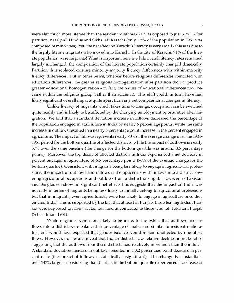
were also much more literate than the resident Muslims - 21% as opposed to just 3.7%. Afterpartition, nearly all Hindus and Sikhs left Karachi (only 1.5% of the population in 1951 wascomposed of minorities). Yet, the net effect on Karachi’s literacy is very small - this was due tothe highly literate migrants who moved into Karachi. In the city of Karachi, 91% of the liter-ate population were migrants! What is important here is while overall literacy rates remainedlargely unchanged, the composition of the literate population certainly changed drastically.Partition thus replaced existing minority-majority literacy differences with within-majorityliteracy differences. Put in other terms, whereas before religious differences coincided witheducation differences, the greater religious homogenization after partition did not producegreater educational homogenization - in fact, the nature of educational differences now be-came within the religious group (rather than across it). This shift could, in turn, have hadlikely significant overall impacts quite apart from any net compositional changes in literacy.
Unlike literacy of migrants which takes time to change, occupation can be switchedquite readily and is likely to be affected by the changing employment opprtunities after mi-gration. We find that a standard deviation increase in inflows decreased the percentage ofthe population engaged in agriculture in India by nearly 6 percentage points, while the sameincrease in outflows resulted in a nearly 5 percentage point increase in the percent engaged inagriculture. The impact of inflows represents nearly 70% of the average change over the 1931-1951 period for the bottom quartile of affected districts, while the impact of outflows is nearly57% over the same baseline (the change for the bottom quartile was around 8.5 percentagepoints). Moreover, the top decile of affected districts in India experienced a net decrease inpercent engaged in agriculture of 6.5 percentage points (76% of the average change for thebottom quartile). Consistent with migrants being less likely to engage in agricultural profes-sions, the impact of outflows and inflows is the opposite - with inflows into a district low-ering agricultural occupations and outflows from a district raising it. However, as Pakistanand Bangladesh show no significant net effects this suggests that the impact on India wasnot only in terms of migrants being less likely to initially belong to agricultural professionsbut that in-migrants, even agriculturists, were less likely to engage in agriculture once theyentered India. This is supported by the fact that at least in Punjab, those leaving Indian Pun-jab were supposed to have vacated less land as compared to those who left Pakistani Punjab(Schechtman, 1951).
While migrants were more likely to be male, to the extent that outflows and in-flows into a district were balanced in percentage of males and similar to resident male ra-tios, one would have expected that gender balance would remain unaffected by migratoryflows. However, our results reveal that Indian districts saw relative declines in male ratiossuggesting that the outflows from these districts had relatively more men than the inflows.A standard deviation increase in outflows resulted in a 0.2 percentage point decrease in per-cent male (the impact of inflows is statistically insignificant). This change is substantial -over 143% larger - considering that districts in the bottom quartile experienced a decrease of
6 BHARADWAJ, KHWAJA & MIAN
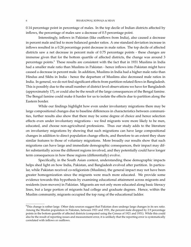
0.14 percentage point in percentage of males. In the top decile of Indian districts affected byinflows, the percentage of males saw a decrease of 0.5 percentage point.
Interestingly, inflows in Pakistan (like outflows from India), also caused a decreasein percent male and led to more balanced gender ratios. A one standard deviation increase ininflows resulted in a 0.24 percentage point decrease in male ratios. The top decile of affecteddistricts saw a net decrease in percent male of 0.75 percentage points - these changes areimmense given that for the bottom quartile of affected districts, the change was around 3percentage points.8 These results are consistent with the fact that in 1931 Muslims in Indiahad a smaller male ratio than Muslims in Pakistan - hence inflows into Pakistan might havecaused a decrease in percent male. In addition, Muslims in India had a higher male ratio thanHindus and Sikhs in India - hence the departure of Muslims also decreased male ratios inIndia. In general, we do not find significant effects from partition-related flows in Bangladesh.This is possibly due to the small number of district level observations we have for Bangladesh(approximately 17), or could also be the result of the large consequences of the Bengal famine.The Bengal famine could make it harder for us to isolate the effects due to partition along theEastern border.
While our findings highlight how even under involuntary migrations there may belarge compositional changes due to baseline differences in characteristics between communi-ties, further results also show that there may be some degree of choice and hence selectioneffects even under involuntary migrations - we find migrants were more likely to be men,educated, and choose non-agricultural professions. Thus our study adds to the literatureon involuntary migrations by showing that such migrations can have large compositionalchanges in addition to direct population change effects, and therefore to an extent they sharesimilar features to those of voluntary migrations. More broadly our results show that suchmigrations can have large and immediate demographic consequences, their impact may dif-fer substantially across the different regions involved, and they potentially could have longerterm consequences in how these regions (differentially) evolve.
Specifically, in the South Asian context, understanding these demographic impactshelps shed light on how India, Pakistan, and Bangladesh evolved after partition. In particu-lar, while Pakistan received co-religionists (Muslims), the general impact may not have beengreater homogenization since the migrants were much more educated. We provide someevidence towards this hypothesis by examining educational attainment across migrants andresidents (non-movers) in Pakistan. Migrants are not only more educated along basic literacylines, but a large portion of migrants had college and graduate degrees. Hence, within theMuslim community, migrants occupied the top rung of the educational ladder.
8This change is rather large. Other data sources suggest that Pakistan does undergo large changes in its sex ratio.Among the Muslim population in Pakistan, between 1921 and 1931, the percent male dropped by 2.9 percentagepoints in the bottom quartile of affected districts (computed using the Census of 1921 and 1931). While this couldalso be the result of reporting issues and measurement error, it is unlikely that the reporting error is systematicallycorrelated with inflows or outflows.

THE PARTITION OF INDIA: DEMOGRAPHIC CONSEQUENCES 7
By presenting such quantitative results, our work also hopes to complement the ma-jor body of work dealing with the Indian partition that has mostly been qualitative. Generaltexts (Bose & Jalal 1998, Brass 1990, Sarkar 1993, Kudaisya & Yong Tan 2000), anecdotal ac-counts (Butalia 2000, Shahid et al 1993), urban sociological work (Bopegamage 1957, Qadeer1957), and fiction (Ghosh 1988, Manto 1997) form the large body of such work. The earliestattempt at an analytical view of the partition is a work by C.N. Vakil that focuses on a broadrange of issues from the actual migration to irrigation, banking, and finance. However, themajority of the book tends to be more "documentary than analytical" (Basch, 1952).
Our work, along with recent work (Hill et. al., 2005), complements the existing lit-erature by taking a quantitative approach that relies on analyzing disaggregated census datafrom the pre and post-partition period. Hill et. al. (2005) undertake a detailed demographicanalysis of Bengal and Punjab during the partition. Their work focusing on Bengal discoversa major slowdown in population growth between 1941- 1951 that cannot be explained com-pletely by partition and probably reflects mortality due to the Bengal Famine. Their workon Punjab puts the number of unrecorded migrants (or those dead) during partition to bearound 2.2 to 2.9 million. Leaning et al (2005) in an ongoing work examine partition and itsimpact on public health outcomes. Our current study, by examining most of British India,intends to present a complete picture of the migratory flows during partition. By focusing onthe district level we develop a more detailed understanding of these flows and, in particular,examine how the flows impacted the demographics of sending and receiving communities.
The paper is organized as follows - Section 2 discusses the methodology and dataused. Section 3 contains results dealing with education, occupation, and gender respectively.Section 4 provides discussion and Section 5 concludes.
2. DATA AND METHODOLOGY
This section details the data and methodology employed and highlights some of theresults from our previous work that are relevant to this paper.
2.1. Data
The data we use in this paper is from the Census of India 1931,9 and the Census ofIndia and Pakistan 1951. The migration (inflows) variable was directly collected by the censusfor both countries in 1951. There was a specific question that asked whether a person hadmoved due to the partition. Measuring outflows is much harder, for we cannot obtain thisdirectly from any data source. As a result, we resort to various methods to impute outflowsusing census data. A quick example recreated from BKM (2008) helps illustrate the basic ideabehind constructing this variable.
Suppose that an Indian district had 100,000 Muslims in the 1931 census. The 1951census shows that this district had 50,000 Muslims. Suppose the expected growth rate for
9We choose to not use the Census of 1941 for various reasons. These reasons are outlined in detail in BKM 2008.One major reason is its incomplete tabulation due to World War II.
8 BHARADWAJ, KHWAJA & MIAN
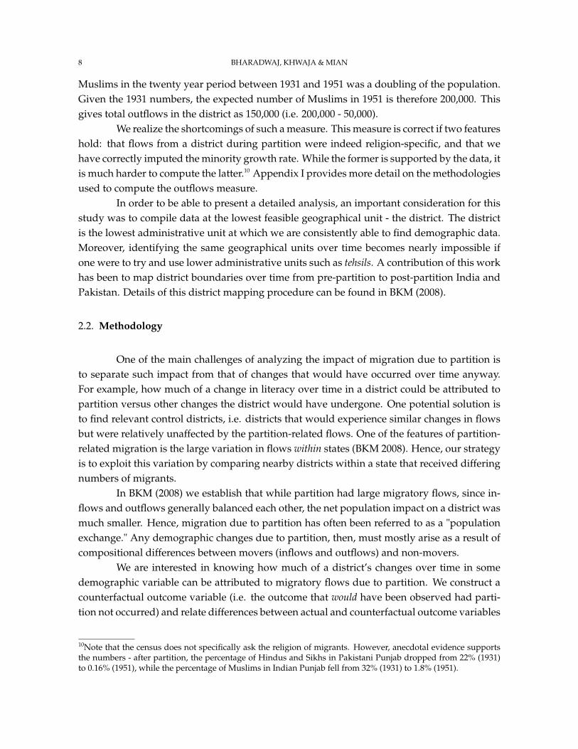
Muslims in the twenty year period between 1931 and 1951 was a doubling of the population.Given the 1931 numbers, the expected number of Muslims in 1951 is therefore 200,000. Thisgives total outflows in the district as 150,000 (i.e. 200,000 - 50,000).
We realize the shortcomings of such a measure. This measure is correct if two featureshold: that flows from a district during partition were indeed religion-specific, and that wehave correctly imputed the minority growth rate. While the former is supported by the data, itis much harder to compute the latter.10 Appendix I provides more detail on the methodologiesused to compute the outflows measure.
In order to be able to present a detailed analysis, an important consideration for thisstudy was to compile data at the lowest feasible geographical unit - the district. The districtis the lowest administrative unit at which we are consistently able to find demographic data.Moreover, identifying the same geographical units over time becomes nearly impossible ifone were to try and use lower administrative units such as tehsils. A contribution of this workhas been to map district boundaries over time from pre-partition to post-partition India andPakistan. Details of this district mapping procedure can be found in BKM (2008).
2.2. Methodology
One of the main challenges of analyzing the impact of migration due to partition isto separate such impact from that of changes that would have occurred over time anyway.For example, how much of a change in literacy over time in a district could be attributed topartition versus other changes the district would have undergone. One potential solution isto find relevant control districts, i.e. districts that would experience similar changes in flowsbut were relatively unaffected by the partition-related flows. One of the features of partition-related migration is the large variation in flows within states (BKM 2008). Hence, our strategyis to exploit this variation by comparing nearby districts within a state that received differingnumbers of migrants.
In BKM (2008) we establish that while partition had large migratory flows, since in-flows and outflows generally balanced each other, the net population impact on a district wasmuch smaller. Hence, migration due to partition has often been referred to as a "populationexchange." Any demographic changes due to partition, then, must mostly arise as a result ofcompositional differences between movers (inflows and outflows) and non-movers.
We are interested in knowing how much of a district’s changes over time in somedemographic variable can be attributed to migratory flows due to partition. We construct acounterfactual outcome variable (i.e. the outcome that would have been observed had parti-tion not occurred) and relate differences between actual and counterfactual outcome variables
10Note that the census does not specifically ask the religion of migrants. However, anecdotal evidence supportsthe numbers - after partition, the percentage of Hindus and Sikhs in Pakistani Punjab dropped from 22% (1931)to 0.16% (1951), while the percentage of Muslims in Indian Punjab fell from 32% (1931) to 1.8% (1951).
THE PARTITION OF INDIA: DEMOGRAPHIC CONSEQUENCES 9
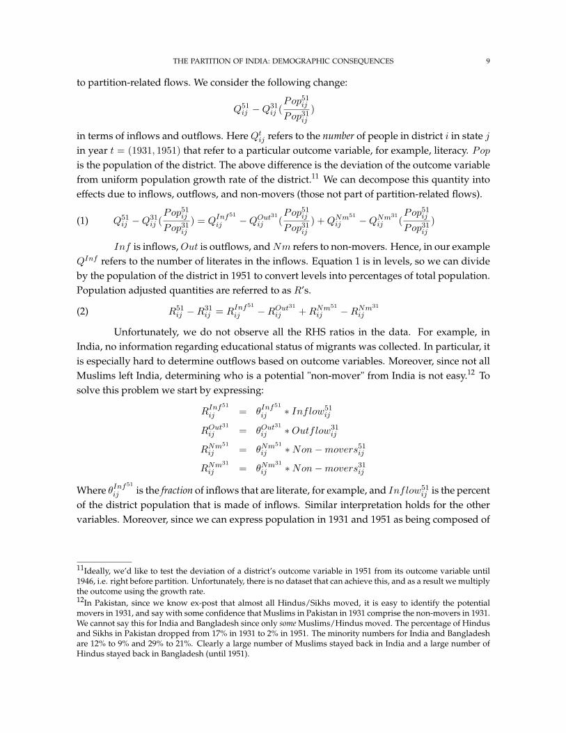
to partition-related flows. We consider the following change:
Q51ij −Q31
ij (Pop51
ij
Pop31ij
)
in terms of inflows and outflows. Here Qtij refers to the number of people in district i in state j
in year t = (1931, 1951) that refer to a particular outcome variable, for example, literacy. Popis the population of the district. The above difference is the deviation of the outcome variablefrom uniform population growth rate of the district.11 We can decompose this quantity intoeffects due to inflows, outflows, and non-movers (those not part of partition-related flows).
Q51ij −Q31
ij (Pop51
ij
Pop31ij
) = QInf51
ij −QOut31
ij (Pop51
ij
Pop31ij
) +QNm51
ij −QNm31
ij (Pop51
ij
Pop31ij
)(1)
Inf is inflows,Out is outflows, andNm refers to non-movers. Hence, in our exampleQInf refers to the number of literates in the inflows. Equation 1 is in levels, so we can divideby the population of the district in 1951 to convert levels into percentages of total population.Population adjusted quantities are referred to as R’s.
R51ij −R31
ij = RInf51
ij −ROut31
ij +RNm51
ij −RNm31
ij(2)
Unfortunately, we do not observe all the RHS ratios in the data. For example, inIndia, no information regarding educational status of migrants was collected. In particular, itis especially hard to determine outflows based on outcome variables. Moreover, since not allMuslims left India, determining who is a potential "non-mover" from India is not easy.12 Tosolve this problem we start by expressing:
RInf51
ij = θInf51
ij ∗ Inflow51ij
ROut31
ij = θOut31
ij ∗Outflow31ij
RNm51
ij = θNm51
ij ∗Non−movers51ij
RNm31
ij = θNm31
ij ∗Non−movers31ij
Where θInf51
ij is the fraction of inflows that are literate, for example, and Inflow51ij is the percent
of the district population that is made of inflows. Similar interpretation holds for the othervariables. Moreover, since we can express population in 1931 and 1951 as being composed of
11Ideally, we’d like to test the deviation of a district’s outcome variable in 1951 from its outcome variable until1946, i.e. right before partition. Unfortunately, there is no dataset that can achieve this, and as a result we multiplythe outcome using the growth rate.12In Pakistan, since we know ex-post that almost all Hindus/Sikhs moved, it is easy to identify the potentialmovers in 1931, and say with some confidence that Muslims in Pakistan in 1931 comprise the non-movers in 1931.We cannot say this for India and Bangladesh since only some Muslims/Hindus moved. The percentage of Hindusand Sikhs in Pakistan dropped from 17% in 1931 to 2% in 1951. The minority numbers for India and Bangladeshare 12% to 9% and 29% to 21%. Clearly a large number of Muslims stayed back in India and a large number ofHindus stayed back in Bangladesh (until 1951).
10 BHARADWAJ, KHWAJA & MIAN
inflows and non-movers, and outflows and non-movers respectively:
RNm51
ij = 1−RInf51
ij
RNm31
ij = 1−ROut31
ij
Rewriting Equation 2 using the above identities yields:
R51ij −R31
ij = (θInf51
ij − θNm51
ij ) ∗ Inflow51ij − (θOut31
ij − θNm31
ij ) ∗Outflow31ij(3)
+θNm51
ij − θNm31
ij
For notational simplicity, we rewrite Equation 4 as:
R51ij −R31
ij = βij ∗ Inflow51ij − γij ∗Outflow31
ij + εij(4)
For the most part, we cannot observe θNm51
ij or θNm31
ij and hence it forms part of the error termin the empirically estimated equation. Empirically, we can only estimate:
R51ij −R31
ij = β ∗ Inflow51ij + γ ∗Outflow31
ij + φij(5)
Since we have only 1 observation per district, clearly we cannot estimate district specific ef-fects in a regression framework. In fact, since we estimate these equations at the countrylevel, our β’s are country specific coefficients.13 The main problem in estimating Equation 5is if migrants decide which district to move into based on the growth rate of non-movers inthat particular district, then φij (which contains the term θNm51
ij − θNm31
ij ) will be correlatedwith Inflowij , and the estimated β will be biased. If the growth of the outcome variableamong non-movers in any way induces migration to (or from) that district, then β and γ
are biased. Suppose migrants choose to go to districts that are growing faster. Moreover, iffaster growing districts transition to adopt more non-agricultural occupations independentlyof migratory flows, by not observing this “growth” we are wrongly attributing changes in theoccupational structure of the district to migratory flows. We attempt to mitigate this problemby introducing a state fixed effect in Equation 5. By introducing a state fixed effect, we arenow comparing districts within a state that received different amounts of migrants. The as-sumption needed to rid β and γ of bias is that within a state, migrants did not choose districtsbased on growth of residents along a particular outcome variable.
Since one of the main concerns is that changes in θNm51
ij − θNm31
ij might be correlatedboth with migratory flows as well as the outcome variable of interest, rather than relyingcompletely on the state fixed effect we include proxies for (θNm51
ij − θNm31
ij ). For example inPakistan, we can compute this quantity quite precisely since we can strongly predict in 1931those who eventually left in 1951 (as noted above, almost all Hindus and Sikhs left Pakistan)- hence θNm31
ij is quite obvious in the case of Pakistan. For India and Bangladesh we proxy for
(θNm51
ij − θNm31
ij ) by using (θMaj31
ij − θMaj21
ij ), which is the difference in fraction belonging tothe outcome variable among the majority population between 1931 and 1921. The idea is to
13Instead of a uniform β, one can think of this as βc

THE PARTITION OF INDIA: DEMOGRAPHIC CONSEQUENCES 11
capture the growth of non-movers in districts (state fixed effects do not capture time-varyinggrowth). The final estimating regression is:
R51ij −R31
ij = βInflow51ij + γOutflow31
ij + ηSj + δXij + uij(6)
Sj is the state fixed effect and Xij are various controls used to mitigate the omitted variablebias problem.14
While we attempt to mitigate this problem by including growth of non-mover prox-ies, there might still be unobservables that influence both migration and the outcome variable.There is some evidence that selective migration might not be that important in this context.In BKM (2008) we provide evidence of "replacement" of outgoing migrants with incomingmigrants that was facilitated by the government. The fact that the government was trying toplace people in areas where there was land available (Kudaisya and Yong Tan, 2000) perhapsmitigates the selection issue to some extent. Moreover, the actual location of the boundarylines were kept a secret until after Independence (Kudaisya and Yong Tan, 2000). Hence,there was a surprise element to the boundary line location, giving people less time to selec-tively migrate.15
3. RESULTS
The outcomes we analyze are literacy, occupation structure, and gender ratios. Foreach outcome, we will first discuss differences between incoming migrants and residents forthe relevant outcome variable (βij from above where such information is available), and thenmove on to presenting the results from estimating Equation 6.
3.1. Literacy
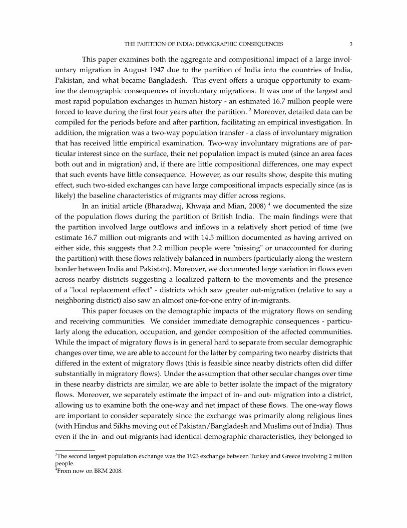
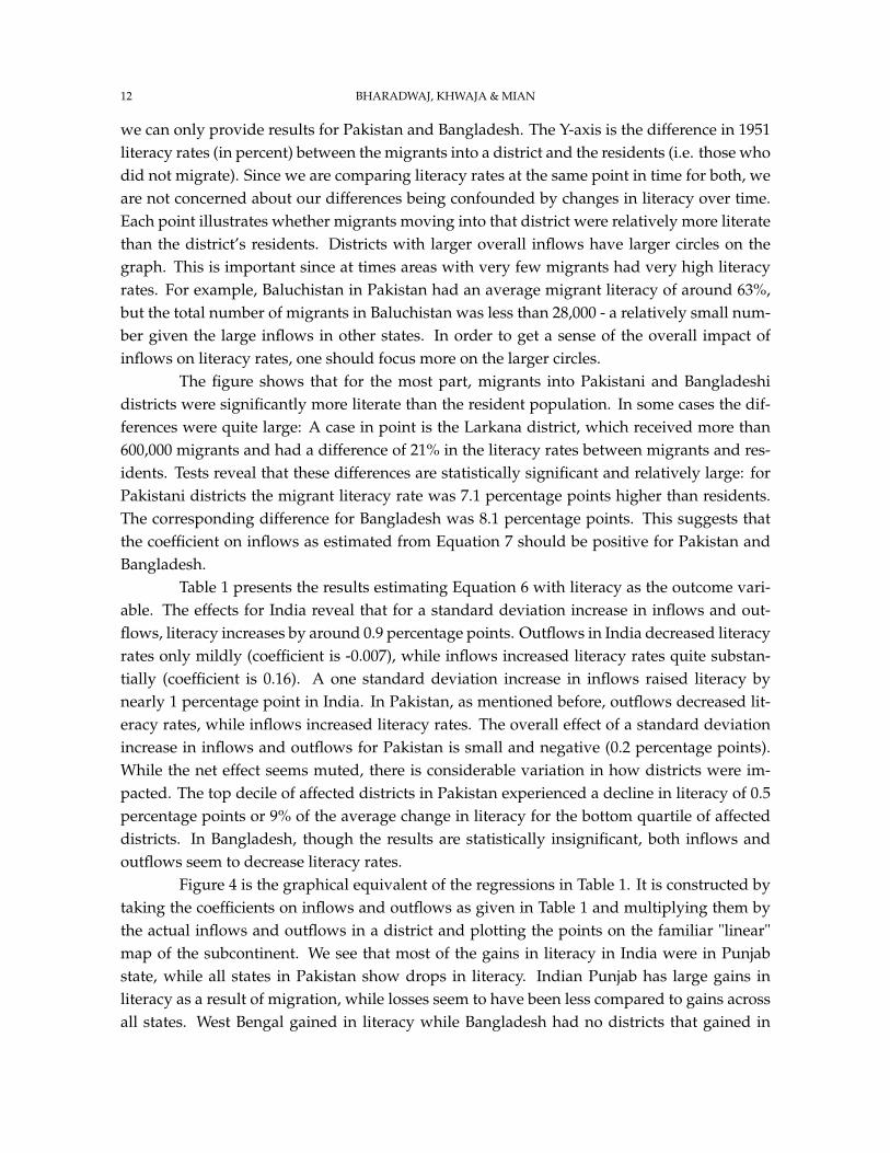
How did migrants compare to residents in terms of their educational background?The anecdotal evidence from Pakistan, especially accounts from Karachi, suggest that mi-grants were more educated. Figure 1 illustrates this for each district using a "linear" map ofBritish India.16 Since data on migrant literacy for India was not tabulated in the 1951 census,
14In estimating Equation 6 we use outflows relative to the 1951 population. This is because we compute outflowsin 1951 units so it only makes sense to use outflows as a percentage of 1951 population. This is unlikely to lead toany bias if the out-migrant population grew at the same rate as the overall population. Given that out-migrantsfrom a country tended to be religion specific, we can check to see if the growth rate of Muslims and non-Muslimsdiffered. The table on growth rates by religion in Appendix 1 confirms that Hindus and Muslims did indeedgrow at different rates. However, the ratio of Muslim or Hindu growth to overall population growth is almost1 in all years. This implies that using outflows relative to 1951 population while estimating Equation 6 does notmechanically change the magnitudes on γ.15In BKM (2008), we note that distance to the border within a state played an insignificant role in determiningwhere migrants went.16Since we will make use of such figures subsequently as well, it is important to explain this more carefully. Eachpoint on the figure represents a particular district. The X-axis of this graph labels the state these districts belongto (thus all districts in a given state are plotted along the same vertical line). States are roughly organized fromwest to east within each country so the graph is roughly akin to converting a map of the region into a single line"map." The western and eastern borders are plotted as vertical lines for reference. Note that the distance betweenstates in the figure does not reflect the actual distance between them.
12 BHARADWAJ, KHWAJA & MIAN
we can only provide results for Pakistan and Bangladesh. The Y-axis is the difference in 1951literacy rates (in percent) between the migrants into a district and the residents (i.e. those whodid not migrate). Since we are comparing literacy rates at the same point in time for both, weare not concerned about our differences being confounded by changes in literacy over time.Each point illustrates whether migrants moving into that district were relatively more literatethan the district’s residents. Districts with larger overall inflows have larger circles on thegraph. This is important since at times areas with very few migrants had very high literacyrates. For example, Baluchistan in Pakistan had an average migrant literacy of around 63%,but the total number of migrants in Baluchistan was less than 28,000 - a relatively small num-ber given the large inflows in other states. In order to get a sense of the overall impact ofinflows on literacy rates, one should focus more on the larger circles.
The figure shows that for the most part, migrants into Pakistani and Bangladeshidistricts were significantly more literate than the resident population. In some cases the dif-ferences were quite large: A case in point is the Larkana district, which received more than600,000 migrants and had a difference of 21% in the literacy rates between migrants and res-idents. Tests reveal that these differences are statistically significant and relatively large: forPakistani districts the migrant literacy rate was 7.1 percentage points higher than residents.The corresponding difference for Bangladesh was 8.1 percentage points. This suggests thatthe coefficient on inflows as estimated from Equation 7 should be positive for Pakistan andBangladesh.
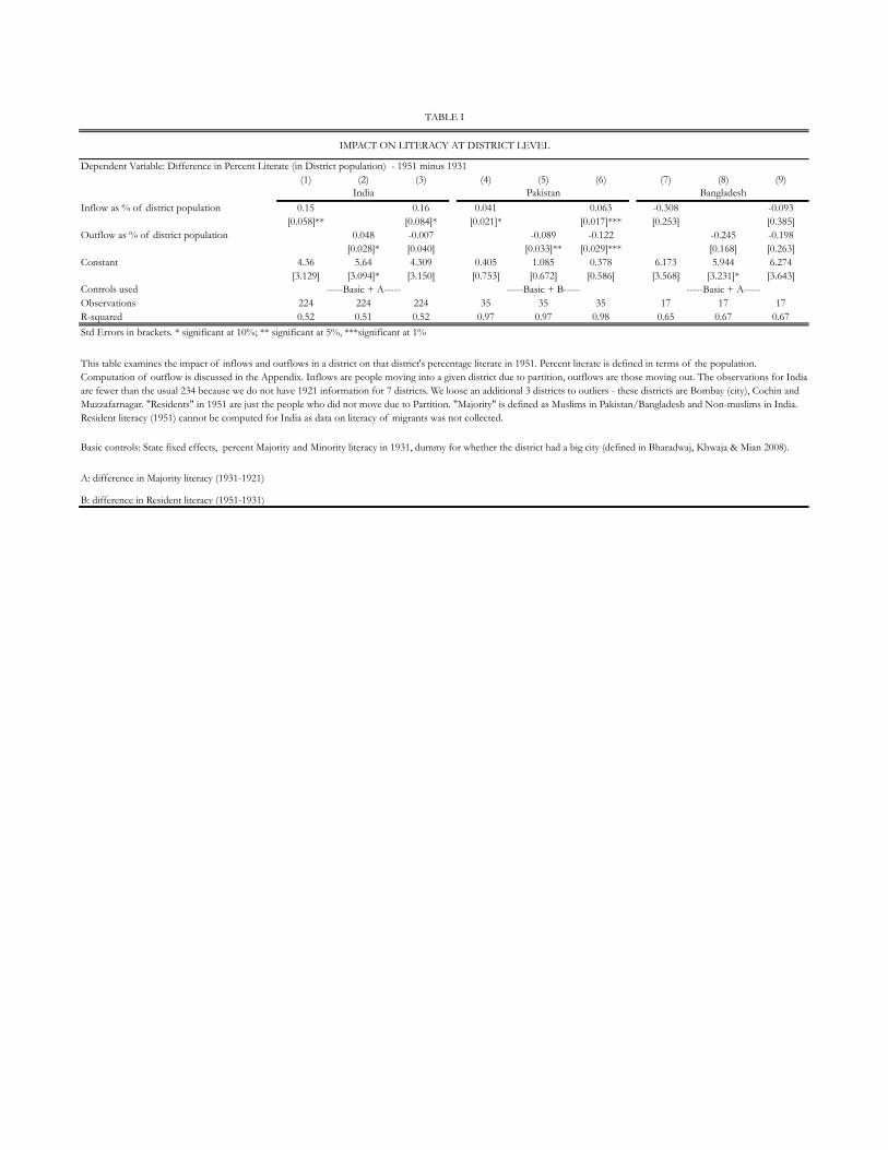
Table 1 presents the results estimating Equation 6 with literacy as the outcome vari-able. The effects for India reveal that for a standard deviation increase in inflows and out-flows, literacy increases by around 0.9 percentage points. Outflows in India decreased literacyrates only mildly (coefficient is -0.007), while inflows increased literacy rates quite substan-tially (coefficient is 0.16). A one standard deviation increase in inflows raised literacy bynearly 1 percentage point in India. In Pakistan, as mentioned before, outflows decreased lit-eracy rates, while inflows increased literacy rates. The overall effect of a standard deviationincrease in inflows and outflows for Pakistan is small and negative (0.2 percentage points).While the net effect seems muted, there is considerable variation in how districts were im-pacted. The top decile of affected districts in Pakistan experienced a decline in literacy of 0.5percentage points or 9% of the average change in literacy for the bottom quartile of affecteddistricts. In Bangladesh, though the results are statistically insignificant, both inflows andoutflows seem to decrease literacy rates.
Figure 4 is the graphical equivalent of the regressions in Table 1. It is constructed bytaking the coefficients on inflows and outflows as given in Table 1 and multiplying them bythe actual inflows and outflows in a district and plotting the points on the familiar "linear"map of the subcontinent. We see that most of the gains in literacy in India were in Punjabstate, while all states in Pakistan show drops in literacy. Indian Punjab has large gains inliteracy as a result of migration, while losses seem to have been less compared to gains acrossall states. West Bengal gained in literacy while Bangladesh had no districts that gained in
THE PARTITION OF INDIA: DEMOGRAPHIC CONSEQUENCES 13
literacy. The above analysis is confirmed in Figure 2.1, which plots the education of minorityand majority groups in 1931. We clearly see that minority groups were more educated thanthe majority in each country. Hence, outflows should decrease literacy, while inflows couldincrease literacy.
As a check, since we know the βij ’s for Pakistan and Bangladesh, we can checkwhether a weighted average17 of the βij ’s corresponds to the β as estimated in the regres-sion. For Pakistan, a weighted average of the βij ’s does match up somewhat to the coefficientsuggested by the regression (the weighted average suggests a coefficient of around 0.0710,while the regression coefficient is 0.063). For Bangladesh this is not the case. The weightedaverage suggests a coefficient of 0.08 while the actual coefficient is -0.093, though it is statis-tically insignificant. This could be the result of the regression not being able to capture theselection process of the migrants or the confounding nature of the Bengal famine. However, itseems unlikely that the selection process of migrants would vary vastly between the Westernand Eastern border. Hence, the results in Bangladesh are more likely to be confounded by theBengal famine that affected the country just a few years prior to partition than some form ofomitted variable bias.
As an aside, we can also examine whether literate migrants were more likely to moveto more distant places than illiterate migrants. The details of this analysis can be found inTable III of Appendix II. Not surprisingly, the literate are significantly more likely to move tomore distant and more educated districts as well as to larger cities.
3.2. Occupation
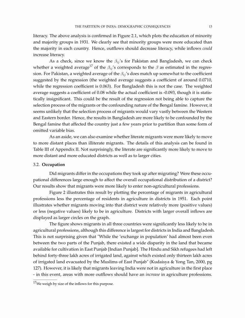
Did migrants differ in the occupations they took up after migrating? Were these occu-pational differences large enough to affect the overall occupational distribution of a district?Our results show that migrants were more likely to enter non-agricultural professions.
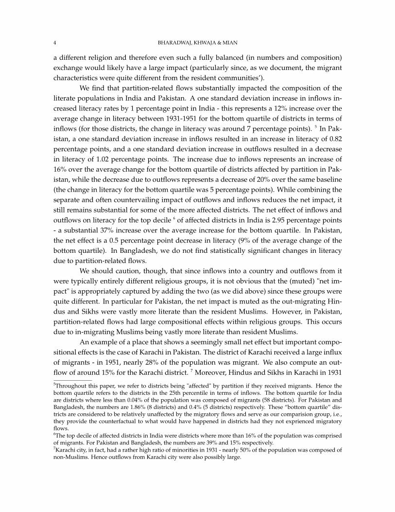
Figure 2 illustrates this result by plotting the percentage of migrants in agriculturalprofessions less the percentage of residents in agriculture in districts in 1951. Each pointillustrates whether migrants moving into that district were relatively more (positive values)or less (negative values) likely to be in agriculture. Districts with larger overall inflows aredisplayed as larger circles on the graph.
The figure shows migrants in all three countries were significantly less likely to be inagricultural professions, although this difference is largest for districts in India and Bangladesh.This is not surprising given that "While the ’exchange in population’ had almost been evenbetween the two parts of the Punjab, there existed a wide disparity in the land that becameavailable for cultivation in East Punjab [Indian Punjab]. The Hindu and Sikh refugees had leftbehind forty-three lakh acres of irrigated land, against which existed only thirteen lakh acresof irrigated land evacuated by the Muslims of East Punjab" (Kudaisya & Yong Tan, 2000, pg127). However, it is likely that migrants leaving India were not in agriculture in the first place- in this event, areas with more outflows should have an increase in agriculture professions.
17We weigh by size of the inflows for this purpose.

14 BHARADWAJ, KHWAJA & MIAN
Still, the difference in land vacated could have more of an effect than that of non-agriculturistsleaving from India. Statistical tests reveal that these differences are indeed large and signifi-cant: for Indian and Bangladeshi districts, the percentage of migrants in agricultural profes-sions was about 28% percentage points lower (compared to residents). The correspondingdifference for Pakistan was only 7 percentage points.
In India, we can explore these relationships even further as the Indian census in 1951provides a more detailed classification of occupation (Table IV, Appendix II). Migrants tendedto engage more in all non-agricultural professions, except the production of raw materials.Moreover, while migrants were less likely to be in agricultural professions, those migrantsthat did go into agriculture were much more likely to own their land or cultivate unownedland, rather than cultivate land owned by someone else.
Table 2 estimates Equation 6 with percentage in agricultural professions as the out-come of interest. The variables of interest are the coefficients on percentage inflows and out-flows. The data for 1931 occupation is incomplete for parts of India and Pakistan. This isdue to non-availability of data as well as some reshaping problems.18 While this leads to lowsample size and therefore lower statistical precision, the districts that experienced the largestinflows (such as those in Punjab and Bengal) are included. Also note that the growth proxyused in this case is the growth in literacy among the majority population between 1921 and1931. This is because information on occupation status by religion was not collected by thecensuses for any of the relevant decades.19 The proxy performs reasonably well in India andPakistan (though not statistically significant) and rather poorly in Bangladesh.
The results show that migratory flows affected the agricultural occupation structurein India. A district which saw one standard deviation increase in inflows (and no outflows)saw a drop of 5.95 percentage points in individuals engaged in agriculture. However, a dis-trict that experienced one standard deviation increase in outflows actually saw agriculturalpropensities rise by an additional 4.79 percentage points. While the net effect is seeminglymuted due to the opposite nature of the impacts of inflows and outflows, the top decile ofaffected districts in India experienced a net decline in percent engaged in agriculture of 6.5percentage points, amounting to nearly 76% of the average change for the bottom quartileof affected districts. Together these two effects suggest that both those who left India andthose who entered it were less likely to be agriculturists/choose agricultural professions.Anecdotal evidence suggests that apart from just constrained choice due to relative short-age of land vacated in India, those leaving Pakistan may have also been more likely to havenon-agricultural vocations. Kudaisya and Tan (2000: pg 179) note that "The economic con-sequences of partition for the city [of Lahore] were severe. Many institutions, banks, andcorporate organizations relocated from the city. The majority of factories closed down and
18Occupation tables are not uniform across the State Censuses. For this reason some states display the occupationtables in a different way than others and some compatibility problems emerge.19There is some information on occupation by religion for Pakistan in 1951. We would still need this informationin 1931 to construct the actual growth figure.
THE PARTITION OF INDIA: DEMOGRAPHIC CONSEQUENCES 15
their plants and buildings were destroyed or abandoned in the disturbances. The bulk of theskilled manpower left, banks and financial institutions ceased functioning, and there was amassive flight of capital."
Figure 5 shows the geographical variation in the impact on agriculture. Indian Pun-jab and Bengal experienced the greatest impacts in terms of decreases in people engaged inagriculture, while the effects are much smaller in Pakistan and Bangladesh.
Again, we can test the validity of our results, by examining the βij ’s for occupationaloutcomes in each country. For India the weighted average of βij is close to the regressioncoefficient in Table 2 (the weighted average suggests a coefficient of -0.68, while the coefficientin the regression is around -0.97). The averages for Pakistan and Bangladesh differ from theregression coefficients, but we spare the details as the regression coefficients themselves arenot significant.
Finally, as an aside, we also examine the mobility of agriculturists versus non-agriculturists.The details of this analysis are in Appendix II (Table V). Migrants entering non-agriculturalprofessions were more likely to migrate to further distances and to larger cities.
3.3. Gender
Did migrants have a different gender composition compared to the general popula-tion? If so, were these differences large enough to have changed overall gender ratios in adistrict?
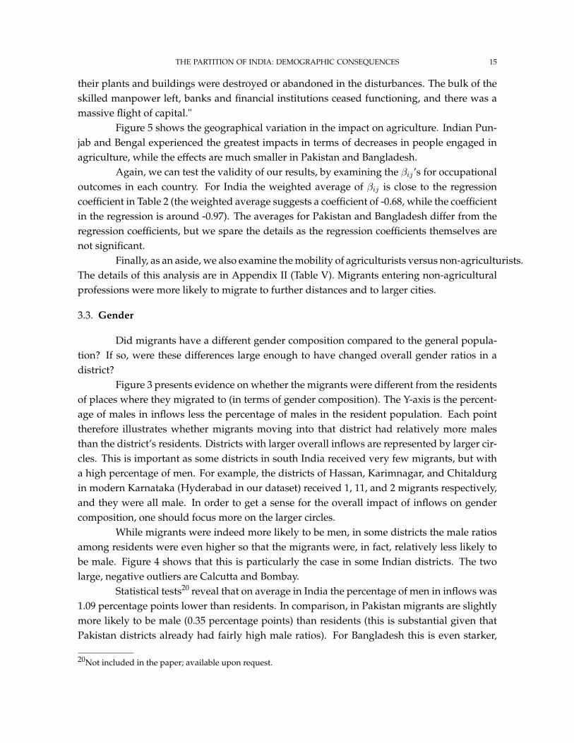
Figure 3 presents evidence on whether the migrants were different from the residentsof places where they migrated to (in terms of gender composition). The Y-axis is the percent-age of males in inflows less the percentage of males in the resident population. Each pointtherefore illustrates whether migrants moving into that district had relatively more malesthan the district’s residents. Districts with larger overall inflows are represented by larger cir-cles. This is important as some districts in south India received very few migrants, but witha high percentage of men. For example, the districts of Hassan, Karimnagar, and Chitaldurgin modern Karnataka (Hyderabad in our dataset) received 1, 11, and 2 migrants respectively,and they were all male. In order to get a sense for the overall impact of inflows on gendercomposition, one should focus more on the larger circles.
While migrants were indeed more likely to be men, in some districts the male ratiosamong residents were even higher so that the migrants were, in fact, relatively less likely tobe male. Figure 4 shows that this is particularly the case in some Indian districts. The twolarge, negative outliers are Calcutta and Bombay.
Statistical tests20 reveal that on average in India the percentage of men in inflows was1.09 percentage points lower than residents. In comparison, in Pakistan migrants are slightlymore likely to be male (0.35 percentage points) than residents (this is substantial given thatPakistan districts already had fairly high male ratios). For Bangladesh this is even starker,
20Not included in the paper; available upon request.
16 BHARADWAJ, KHWAJA & MIAN
with migrants being 2.6 percentage points more likely to be male as compared to the residentsin the districts they migrated to.
Table 3 presents the OLS results of estimating Equation 6 with percent men as theoutcome variable. The results are interesting for India as they suggest areas that experiencedgreater outflows were more likely to see a drop in male ratios: compared to a district that ex-perienced no outflows, a district that saw one standard deviation increase outflows would seethe difference in percentage of men from 1931 to 1951 drop by around 0.20 percentage points(Column 3). In Pakistan, a one standard deviation increase in inflows decreased the differ-ence in percent male by 0.24 percentage points. Outflows from Pakistan tended to increasemale ratios, but the coefficient is rather small and statistically insignificant. The top decileof affected districts in Pakistan experienced a net decrease in percent make of 0.75 percent-age points - this is a fairly substantial change considering that the bottom quartile of affecteddistricts experienced a change in percent male of 3 percentage points over this period. ForBangladesh the overall effect is negative, small in magnitude, and statistically insignificant.These results are consistent with the fact that in 1931 Muslims in India had a smaller male ra-tio than Muslims in Pakistan - hence inflows into Pakistan might cause a decrease in percentmale. In addition, Muslims in India had a higher male ratio than Hindus and Sikhs in India -hence the departure of Muslims also decreased male ratios in India.
Figure 6 shows the geographic variation of impacts on gender ratios. As expected,the biggest changes are close to the border. There are districts in Indian Punjab and Bengalthat experienced decreases in male ratios. We see the same result in Pakistan as well.
The weighted average of the individual βij ’s suggests a coefficient of -0.01 in India(the regression coefficient is -0.003, and statistically insignificant), positive 0.003 for Pakistan(quite different from the regression coefficient of -0.019), and 0.02 for Bangladesh (the regres-sion coefficient is 0.05). Hence, selection bias might be more of an issue in these estimates.
Additionally, we can also examine whether men were more likely to move to moredistant places then women. The details of this analysis are relegated to Appendix II (Table I)but it is worth highlighting that men were more likely to migrate to more distant districts andto larger cities.
4. DISCUSSION: WITHIN MAJORITY DIFFERENCES
As emphasized in the introduction, while aggregate effects of the migratory flowsare mitigated by the counteracting effects of inflows and outflows, they represent importantchanges in the composition of the newly formed countries. Minority-majority differencesalong various lines were likely replaced with within-majority differences. These differencesmay have been particularly salient for Pakistan both because most minority groups migratedout and because of the large differences in attributes such as educational attainment betweenin-migrants and the resident population.
THE PARTITION OF INDIA: DEMOGRAPHIC CONSEQUENCES 17
We first examine these compositional changes along the lines of education status.Owing to greater data availability, we do this for Pakistan only. As mentioned before, mi-grants into Pakistan were vastly more educated than the residents. Among total literate inPakistan in 1951, migrants were approximately 20%. In fact, these differences were not onlyin basic educational measures such as literacy rates, but also in educational attainment in gen-eral (See Table I, Appendix II). If we categorize educational attainment as either attainment ofprimary and middle education (up to class 8) or matriculation (10th class) and higher, we findthat migrants were more educated than residents in Pakistan. The idea that within-Musliminequality increased is seen clearly in that among people with higher degrees (higher than col-lege degrees) migrants were approximately 47%. Unfortunately we cannot compare migranteducation attainment to that of the Hindus and Sikhs who left as we do not have attainmentinformation from 1931.
In addition to the above within-group differences, geographic inequalities arose aseducated migrants tended to concentrate in big cities. Nearly 20% of literate migrants concen-trated in the city of Karachi. Hence Karachi, which in 1931 contributed only 8.9% of total liter-ates in Pakistan, suddenly contributed 20% with most of that increase due to literate migrants.When the geographic concentration is combined with educational attainment differences, theresults show the emergence of Karachi as the center of the migrant elite. Among migrantswith higher degrees, 50% went to Karachi city. The case of Karachi is particularly importantas it was the first capital of independent Pakistan.21 While India may have experienced sim-ilar within-group differences, it is noteworthy that in terms of urban compositional changes,India’s experience differed substantially from Pakistan’s. In India, Hindus in big cities werealready very literate in 1931 - in fact, they were almost as literate as Hindus in Pakistan atthe same time (13.2% as opposed to 16.5%). Muslims in big cities in Pakistan, however, wereless educated than the average migrant into Pakistan in 1951 (20.2% as opposed to 31.5%).Thus, post-partition, when migrants tended to go to larger cities (BKM 2008), the differencesbetween migrants and residences were greater in Pakistan than in India.
Hence, on the surface what looks to be small aggregate changes in population charac-teristics actually hides important compositional and geographic concentration aspects. Whileit is hard to draw long-term implications simply on the basis of these patterns, it is noteworthythat the within-group differences, particularly in urban areas, that arose due to the migratoryflows may have contributed to differences in how the countries evolved. Pakistan experi-enced large within-group changes both because migrants were substantially more educatedand because these differences were even starker in urban areas that likely played a greaterinfluence. In contrast, in India while there were also substantial within-group differences ineducation created due to the migratory flows, these were likely to be less salient overall bothbecause a large fraction of India experienced little migratory flows (and hence a greater frac-tion of the initial minority group remained) and also because the migrant-resident differences
21The capital moved to Rawalpindi in 1958 and then to Islamabad in 1960.
18 BHARADWAJ, KHWAJA & MIAN
were much less stark in Indian cities. These patterns do raise the question of whether theymay have impacted the lines of conflict in India versus Pakistan since the evidence in theensuing decades suggests that while religion remained a salient source of divisions in India,in Pakistan the more significant difference tended to be within Muslims, with migrant statusoften playing an important role. 22
5. CONCLUSION
In this paper we analyzed the aggregate impact of partition-related migration ongender, education, and occupation structure of districts in India, Pakistan, and Bangladesh.We conclude that partition-related flows resulted in an increase in literacy rates in India anda decrease in the percentage of people engaged in agriculture. In Pakistan, while incomingmigrants tended to raise the literacy rates, out migrating Hindus and Sikhs (themselves beingvery literate) tended to reduce total literacy - in sum, there is a decrease in Pakistan’s literacyrate as a result of partition. In addition, these flows led to a decrease in male ratios in Indiaand Pakistan.
Despite the fact that the overall net effects of the flows are muted due to the two-way nature of the flows, there is considerable variation in how districts were affected. Thetop decile of affected districts in each country experienced dramatic changes in its literacyrates, occupation structure and gender ratios. While these effects are important, they are onlyrelevant if they played a role in the later development of these countries. We think partition-related flows were important for the future development of the countries involved for tworeasons.
First, minority-majority differences were replaced with within- majority differences.In the case of Pakistan, the fact that the migrants were vastly more literate and geographicallyconcentrated clearly shaped its political landscape.
It is worth noting that the top leaders in the initial years of Pakistan had all beenMuhajirs [migrants].. . . With . . . their higher levels of education and skills, their rep-resentation in the bureaucratic and political systems, and their assertions of culturalsuperiority, the Muhajirs could not assimilate themselves with the original inhabitantsof Karachi (Kudaisya & Yong Tan, 2000).
Second, at least in the case of India, the increase in people engaged in non-agricultural pro-fessions could have been instrumental in the industrialization process. The long-term conse-quences of these demographic changes for India are harder to determine due to the country’ssize. Perhaps the lack of land for agriculturists spurred growth in the non-agricultural sectorvia decreased supply of agricultural labor supply. It is harder to imagine how the change ingender ratios could have played a role in development.
22While this is also because Pakistan had fewer Hindus/Sikhs left, there are a substantial number of Hindus inSindh and at least anecdotally there seem to be relatively less divisions in Sindh between them and Muslims thanwithin Muslims.

THE PARTITION OF INDIA: DEMOGRAPHIC CONSEQUENCES 19
In subsequent work we also hope to examine other socioeconomic consequences ofthese flows. Moreover, the broader goals of our project are to compile and make availablecomparable demographic and socioeconomic data for the pre and post-partition period thatwould make analytic work on the partition more feasible and attractive to the research com-munity. In turn, such empirical analysis can both be driven by and add to the existing richqualitative literature on the partition.
20 BHARADWAJ, KHWAJA & MIAN
6. REFERENCES
Basch, A. Reviewed Work of Economic Consequences of Divided India by CN Vakil, Ameri-can Economic Review, (1952).
Bharadwaj, P., Khwaja, A., Mian, A. The Big March: Migratory Flows after Partition ofBritish India. Economic and Political Weekly Vol.43, No. 35 (2008).
Bopegamage, A. Delhi: A Study in Urban Sociology, University of Bombay Publica-tions, Sociology Series No. 7 (1957).
Borjas, G. The Economics of Immigration, Journal of Economic Literature, (1994).Borjas, G, Freeman, R & Katz, L. Searching for the Effect of Immigration on the Labor
Market, American Economic Review, (1996).Bose, S & Jalal. A. Modern South Asia: History, Culture, Political Economy New York:
Routledge (1998).Boyer, G., Hatton, T. and O’Rourke, K. The Impact of Emigration on Real Wages in Ireland
1850-1914, CEPR Discussion Papers 854 (1993).Brass, P. The Politics of India since Independence, London: Cambridge University Press
(1990)Butalia U. The Other Side of Silence: Voices from the Partition of India, Duke University
Press (2000).Cheema, P I. The Politics of the Punjab Boundary Award, Heidelberg Papers in South
Asian and Comparative Politics, Working Paper (1), 2000.Cernea, M. The Risks and Reconstruction Model for Resettling Displaced Populations, World
Development (1997).Davis, K. The Population of India and Pakistan, Princeton: Princeton University Press
(1951).Fernandes, W, Das, JC & Rao, S.Displacement and Rehabilitation: An Estimate of Extent
and Prospects, In W. Fernandes and E. Ganguly Thukral, eds., Development, Displacementand Rehabilitation. New Delhi: ISI (1989).
Ghosh, A. The Shadow lines, Bloomsbury (1988).Government of India, Census of India 1931, India: Central publication branch (1933).Government of India, Census of India 1941, Delhi: The Manager of Publications,
(1941-1945).Government of India, Census of India 1951, Delhi: The Manager of Publications,
(1952).Government of Pakistan, Census of Pakistan 1951, Karachi: The Manager of Publica-
tions, (1954-56).Guinnane, Timothy. The Vanishing Irish, Princeton: Princeton University Press (1997).LaLonde, R & Topel, R. Economic Impact of International Migration and the Economic
Performance of Immigrants, In Handbook of Population and Family Economics, edited by MarkRosenzweig and Oded Stark. Amsterdam: Elsevier Science Publishing (1996).

THE PARTITION OF INDIA: DEMOGRAPHIC CONSEQUENCES 21
Hatton, T & Williamson, J. The Age of Mass Migration: Causes and Economic Impact,New York and Oxford: Oxford University Press (1998).
Hatton, T & Williamson, J. What drove the mass migrations from Europe in the late nine-teenth century?, Population and Development Review, (1994).
Hill, K et al. The partition of India: new demographic estimates of associated populationchange International Union for the Scientific Study of Population, International PopulationConference, France, 2005.
Jacobsen, K. Refugees’ Environmental Impact: The Effect of Patterns of Settlemen, Journalof Refugee Studies (1997).
Kudaisya, G & Yong Tan, T. The Aftermath of Partition in South Asia, London: Rout-ledge (2000)
Manto, SH. Mottled Dawn; Fifty Sketches and Stories of Partition, Penguin Books India(1997).
Sarkar, S. Modern India 1885-1947, Basingstoke: Macmillan (1993).Sherwani, L A. The partition of India and Mountbatten, Karachi, Council for Pakistan
Studies (1986).Shahid, S & Major General Hamid. Disasterous Twilight: A Personal Record of the Parti-
tion of India, Trans-Atlantic Publications (1993).Singh A, Moon P, & Khosla D. The Partition Omnibus, London: Oxford University
Press (2001)Srivastava, R & Sasikiran SK. An Overview of Migration in India, its Impacts and Key
Issues, www.livelihoods.org.Sugata,B & Jalal, A. Modern South Asia: History, Culture, Political Economy, London:
Routledge (1998)Qadeer, MA. Lahore: Urban Development in the Third World, Lahore, Vanguard Books
Limited (1983).Vakil, CN. Economic Consequences of Divided India, Bombay: Vora & Co (1950).van Hear, N. The Impact of the Involuntary Mass ’Return’ to Jordan in the Wake of the Gulf
Crisis, International Migration Review (1995).Wallbank, T W. (ed) The partition of India: causes and responsibilities, Boston: Heath
(1966).
22 BHARADWAJ, KHWAJA & MIAN
7. APPENDIX 1
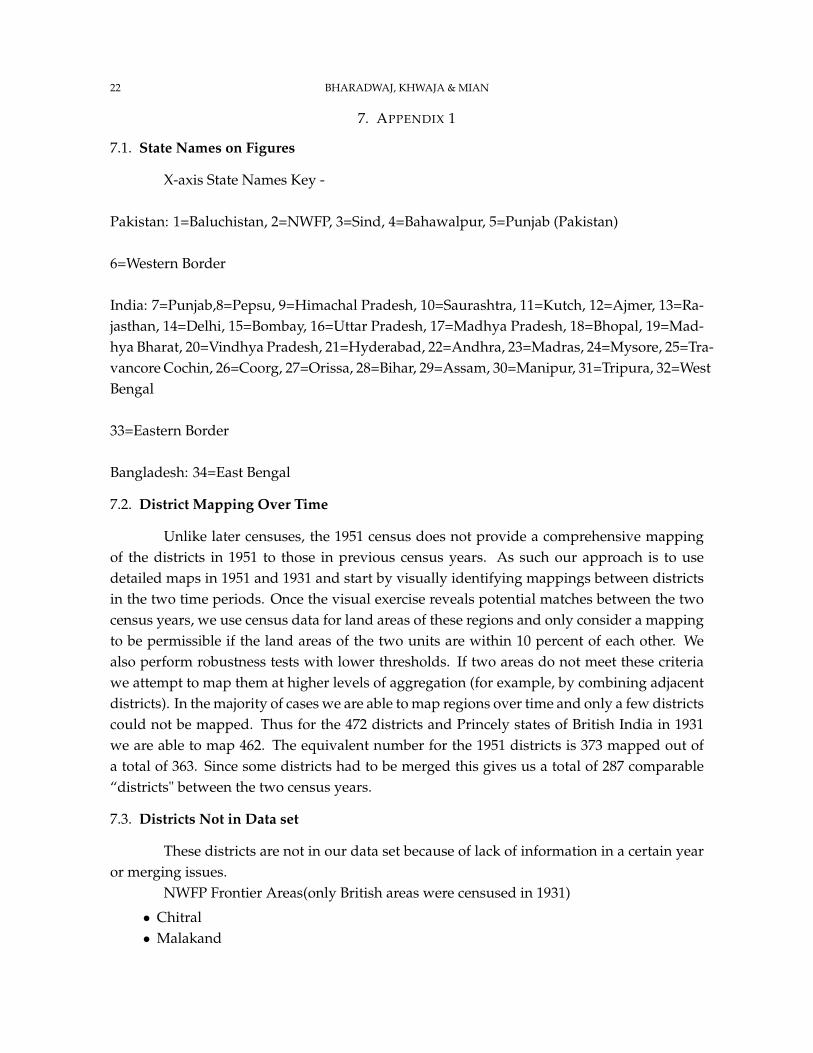
7.1. State Names on Figures
X-axis State Names Key -
Pakistan: 1=Baluchistan, 2=NWFP, 3=Sind, 4=Bahawalpur, 5=Punjab (Pakistan)
6=Western Border
India: 7=Punjab,8=Pepsu, 9=Himachal Pradesh, 10=Saurashtra, 11=Kutch, 12=Ajmer, 13=Ra-jasthan, 14=Delhi, 15=Bombay, 16=Uttar Pradesh, 17=Madhya Pradesh, 18=Bhopal, 19=Mad-hya Bharat, 20=Vindhya Pradesh, 21=Hyderabad, 22=Andhra, 23=Madras, 24=Mysore, 25=Tra-vancore Cochin, 26=Coorg, 27=Orissa, 28=Bihar, 29=Assam, 30=Manipur, 31=Tripura, 32=WestBengal
33=Eastern Border
Bangladesh: 34=East Bengal
7.2. District Mapping Over Time
Unlike later censuses, the 1951 census does not provide a comprehensive mappingof the districts in 1951 to those in previous census years. As such our approach is to usedetailed maps in 1951 and 1931 and start by visually identifying mappings between districtsin the two time periods. Once the visual exercise reveals potential matches between the twocensus years, we use census data for land areas of these regions and only consider a mappingto be permissible if the land areas of the two units are within 10 percent of each other. Wealso perform robustness tests with lower thresholds. If two areas do not meet these criteriawe attempt to map them at higher levels of aggregation (for example, by combining adjacentdistricts). In the majority of cases we are able to map regions over time and only a few districtscould not be mapped. Thus for the 472 districts and Princely states of British India in 1931we are able to map 462. The equivalent number for the 1951 districts is 373 mapped out ofa total of 363. Since some districts had to be merged this gives us a total of 287 comparable“districts" between the two census years.
7.3. Districts Not in Data set
These districts are not in our data set because of lack of information in a certain yearor merging issues.
NWFP Frontier Areas(only British areas were censused in 1931)
• Chitral• Malakand

THE PARTITION OF INDIA: DEMOGRAPHIC CONSEQUENCES 23
• Swat• Dir• North & South Waziristan• Khurran• Khyber
Baluchistan (one area was not censused in 1951)
• Dera Ghazi Khan
Gilgit Agency (not censused)
• Yasin• Kuh Ghizar• Punial• Tangir & Darel• Ishkuman• Gilgit• Chilas• Astor• Hunza & Nagir
Assam Hill/Tribal Areas (not censused in 1951)
• Sadiya Frontier Tract• Khasi and Jaintia Hills
Jammu and Kashmir (not censused in 1951)
• Baramula• Anantnag• Riasi• Udhampur• Chamba• Kathua• Jammu• Punch• Mirpur• Muzaffarabad
Andaman and Nicobar Islands (have missing information in the 1931 census). Sikkim (itsstatus was uncertain in 1951 and was only inducted into state of India in 1975).
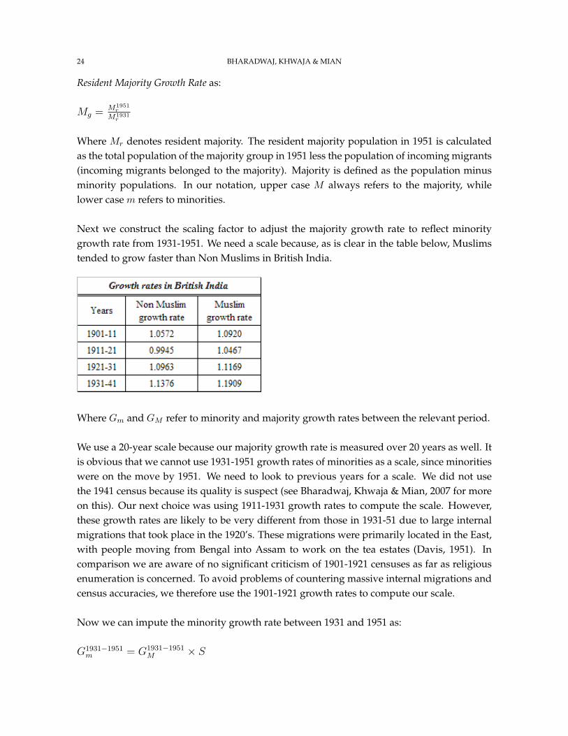
7.4. Computing Outflows
Our method of computing outflows determines expected minority growth rates byre-scaling the growth rates of the majority population during the relevant period (1931-1951).Note that “minorities" in Pakistan are Non-Muslims, while minorities in India are Muslims.“Majority" in India are Non-Muslims, while majority in Pakistan are Muslims. We define the
24 BHARADWAJ, KHWAJA & MIAN
Resident Majority Growth Rate as:
Mg = M1951r
M1931r
Where Mr denotes resident majority. The resident majority population in 1951 is calculatedas the total population of the majority group in 1951 less the population of incoming migrants(incoming migrants belonged to the majority). Majority is defined as the population minusminority populations. In our notation, upper case M always refers to the majority, whilelower case m refers to minorities.
Next we construct the scaling factor to adjust the majority growth rate to reflect minoritygrowth rate from 1931-1951. We need a scale because, as is clear in the table below, Muslimstended to grow faster than Non Muslims in British India.
Where Gm and GM refer to minority and majority growth rates between the relevant period.
We use a 20-year scale because our majority growth rate is measured over 20 years as well. Itis obvious that we cannot use 1931-1951 growth rates of minorities as a scale, since minoritieswere on the move by 1951. We need to look to previous years for a scale. We did not usethe 1941 census because its quality is suspect (see Bharadwaj, Khwaja & Mian, 2007 for moreon this). Our next choice was using 1911-1931 growth rates to compute the scale. However,these growth rates are likely to be very different from those in 1931-51 due to large internalmigrations that took place in the 1920’s. These migrations were primarily located in the East,with people moving from Bengal into Assam to work on the tea estates (Davis, 1951). Incomparison we are aware of no significant criticism of 1901-1921 censuses as far as religiousenumeration is concerned. To avoid problems of countering massive internal migrations andcensus accuracies, we therefore use the 1901-1921 growth rates to compute our scale.
Now we can impute the minority growth rate between 1931 and 1951 as:
G1931−1951m = G1931−1951
M × S

THE PARTITION OF INDIA: DEMOGRAPHIC CONSEQUENCES 25
Finally we can compute the expected number of minorities in 1951.
ˆm1951 = m1931 ×G1931−1951m
Outflow is the number of expected minorities less the actual number of minorities in a givendistrict:
Outflow = ˆm1951 −m1951
The above analysis is computed at the district level with one exception. We do not have1901 census figures at the district level. Hence, we just use the country-wide scale on the1931-51 majority growth rate at the district level.
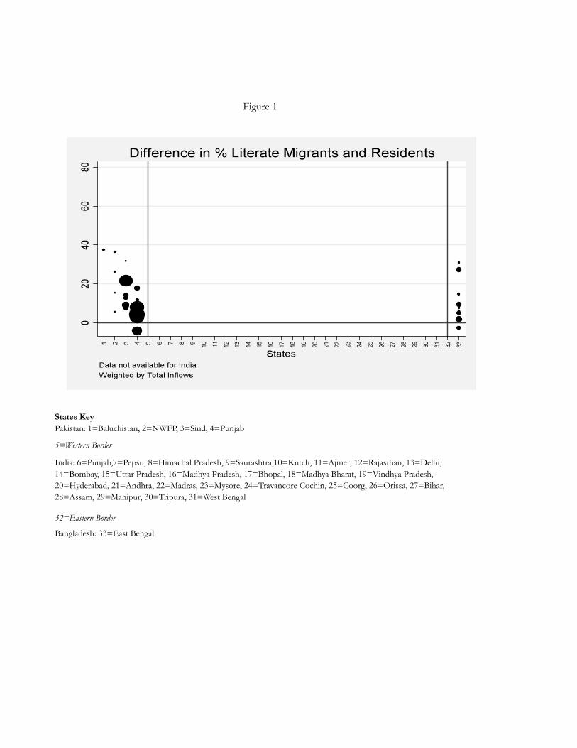
Figure 1
States KeyPakistan: 1=Baluchistan, 2=NWFP, 3=Sind, 4=Punjab
5=Western Border
32=Eastern Border
Bangladesh: 33=East Bengal
India: 6=Punjab,7=Pepsu, 8=Himachal Pradesh, 9=Saurashtra,10=Kutch, 11=Ajmer, 12=Rajasthan, 13=Delhi,
14=Bombay, 15=Uttar Pradesh, 16=Madhya Pradesh, 17=Bhopal, 18=Madhya Bharat, 19=Vindhya Pradesh,
20=Hyderabad, 21=Andhra, 22=Madras, 23=Mysore, 24=Travancore Cochin, 25=Coorg, 26=Orissa, 27=Bihar,
28=Assam, 29=Manipur, 30=Tripura, 31=West Bengal

Figure 1.1
States KeyPakistan: 1=Baluchistan, 2=NWFP, 3=Sind, 4=Punjab
5=Western Border
32=Eastern Border
Bangladesh: 33=East Bengal
India: 6=Punjab,7=Pepsu, 8=Himachal Pradesh, 9=Saurashtra,10=Kutch, 11=Ajmer, 12=Rajasthan, 13=Delhi, 14=Bombay, 15=Uttar Pradesh,
16=Madhya Pradesh, 17=Bhopal, 18=Madhya Bharat, 19=Vindhya Pradesh, 20=Hyderabad, 21=Andhra, 22=Madras, 23=Mysore,
24=Travancore Cochin, 25=Coorg, 26=Orissa, 27=Bihar, 28=Assam, 29=Manipur, 30=Tripura, 31=West Bengal
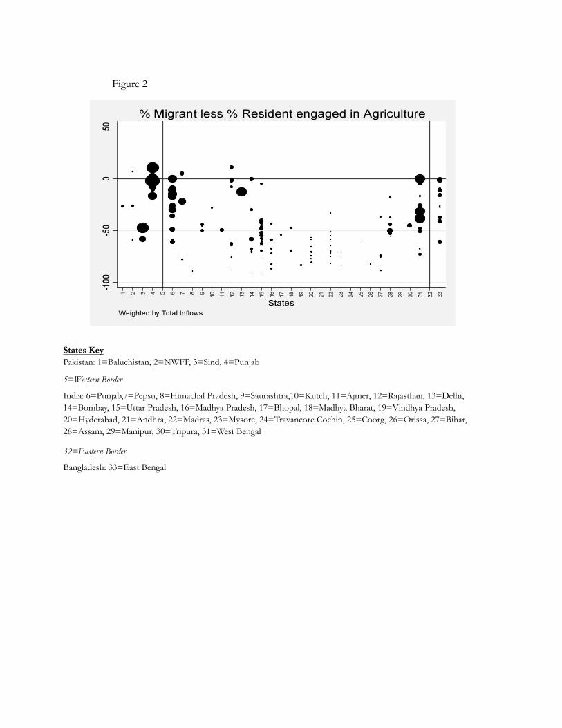
Figure 2
States KeyPakistan: 1=Baluchistan, 2=NWFP, 3=Sind, 4=Punjab
5=Western Border
32=Eastern Border
Bangladesh: 33=East Bengal
India: 6=Punjab,7=Pepsu, 8=Himachal Pradesh, 9=Saurashtra,10=Kutch, 11=Ajmer, 12=Rajasthan, 13=Delhi,
14=Bombay, 15=Uttar Pradesh, 16=Madhya Pradesh, 17=Bhopal, 18=Madhya Bharat, 19=Vindhya Pradesh,
20=Hyderabad, 21=Andhra, 22=Madras, 23=Mysore, 24=Travancore Cochin, 25=Coorg, 26=Orissa, 27=Bihar,
28=Assam, 29=Manipur, 30=Tripura, 31=West Bengal
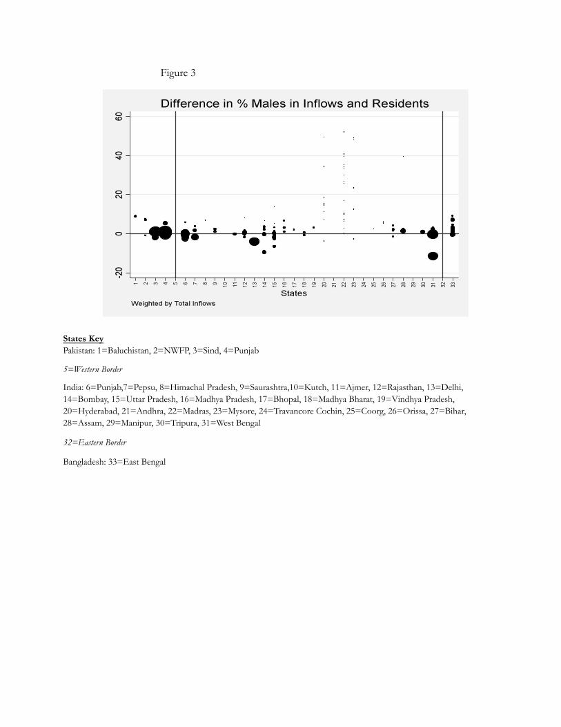
Figure 3
States KeyPakistan: 1=Baluchistan, 2=NWFP, 3=Sind, 4=Punjab
5=Western Border
32=Eastern Border
Bangladesh: 33=East Bengal
India: 6=Punjab,7=Pepsu, 8=Himachal Pradesh, 9=Saurashtra,10=Kutch, 11=Ajmer, 12=Rajasthan, 13=Delhi,
14=Bombay, 15=Uttar Pradesh, 16=Madhya Pradesh, 17=Bhopal, 18=Madhya Bharat, 19=Vindhya Pradesh,
20=Hyderabad, 21=Andhra, 22=Madras, 23=Mysore, 24=Travancore Cochin, 25=Coorg, 26=Orissa, 27=Bihar,
28=Assam, 29=Manipur, 30=Tripura, 31=West Bengal

Figure 4
Graph weighted by total population in 1951
States KeyPakistan: 1=Baluchistan, 2=NWFP, 3=Sind, 4=Punjab
5=Western Border
32=Eastern Border
Bangladesh: 33=East Bengal
India: 6=Punjab,7=Pepsu, 8=Himachal Pradesh, 9=Saurashtra,10=Kutch, 11=Ajmer, 12=Rajasthan, 13=Delhi, 14=Bombay, 15=Uttar Pradesh,
16=Madhya Pradesh, 17=Bhopal, 18=Madhya Bharat, 19=Vindhya Pradesh, 20=Hyderabad, 21=Andhra, 22=Madras, 23=Mysore, 24=Travancore
Cochin, 25=Coorg, 26=Orissa, 27=Bihar, 28=Assam, 29=Manipur, 30=Tripura, 31=West Bengal
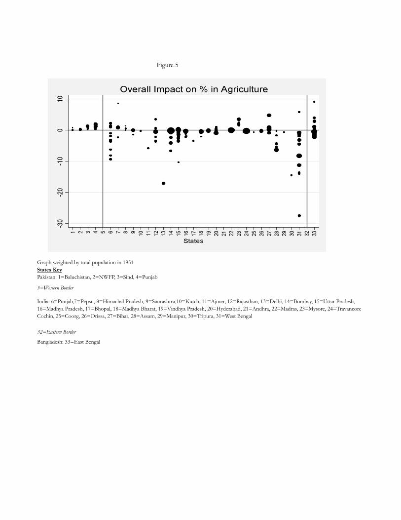
Figure 5
Graph weighted by total population in 1951
States KeyPakistan: 1=Baluchistan, 2=NWFP, 3=Sind, 4=Punjab
5=Western Border
32=Eastern Border
Bangladesh: 33=East Bengal
India: 6=Punjab,7=Pepsu, 8=Himachal Pradesh, 9=Saurashtra,10=Kutch, 11=Ajmer, 12=Rajasthan, 13=Delhi, 14=Bombay, 15=Uttar Pradesh,
16=Madhya Pradesh, 17=Bhopal, 18=Madhya Bharat, 19=Vindhya Pradesh, 20=Hyderabad, 21=Andhra, 22=Madras, 23=Mysore, 24=Travancore
Cochin, 25=Coorg, 26=Orissa, 27=Bihar, 28=Assam, 29=Manipur, 30=Tripura, 31=West Bengal
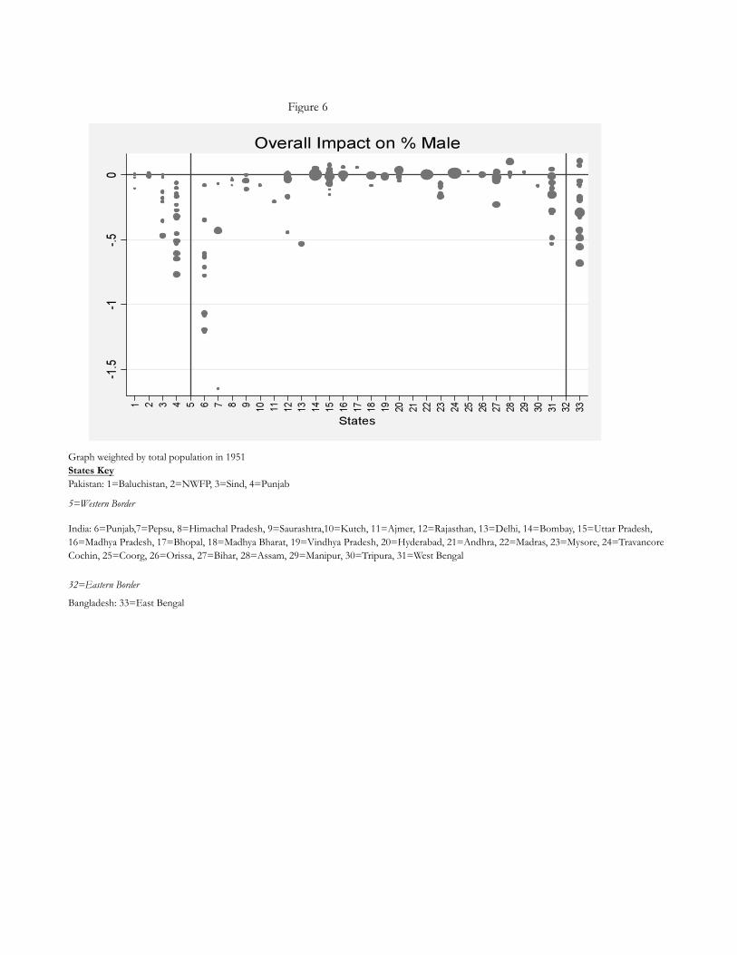
Figure 6
Graph weighted by total population in 1951
States KeyPakistan: 1=Baluchistan, 2=NWFP, 3=Sind, 4=Punjab
5=Western Border
32=Eastern Border
Bangladesh: 33=East Bengal
India: 6=Punjab,7=Pepsu, 8=Himachal Pradesh, 9=Saurashtra,10=Kutch, 11=Ajmer, 12=Rajasthan, 13=Delhi, 14=Bombay, 15=Uttar Pradesh,
16=Madhya Pradesh, 17=Bhopal, 18=Madhya Bharat, 19=Vindhya Pradesh, 20=Hyderabad, 21=Andhra, 22=Madras, 23=Mysore, 24=Travancore
Cochin, 25=Coorg, 26=Orissa, 27=Bihar, 28=Assam, 29=Manipur, 30=Tripura, 31=West Bengal
Mean Std Dev Mean Std Dev Mean Std Dev
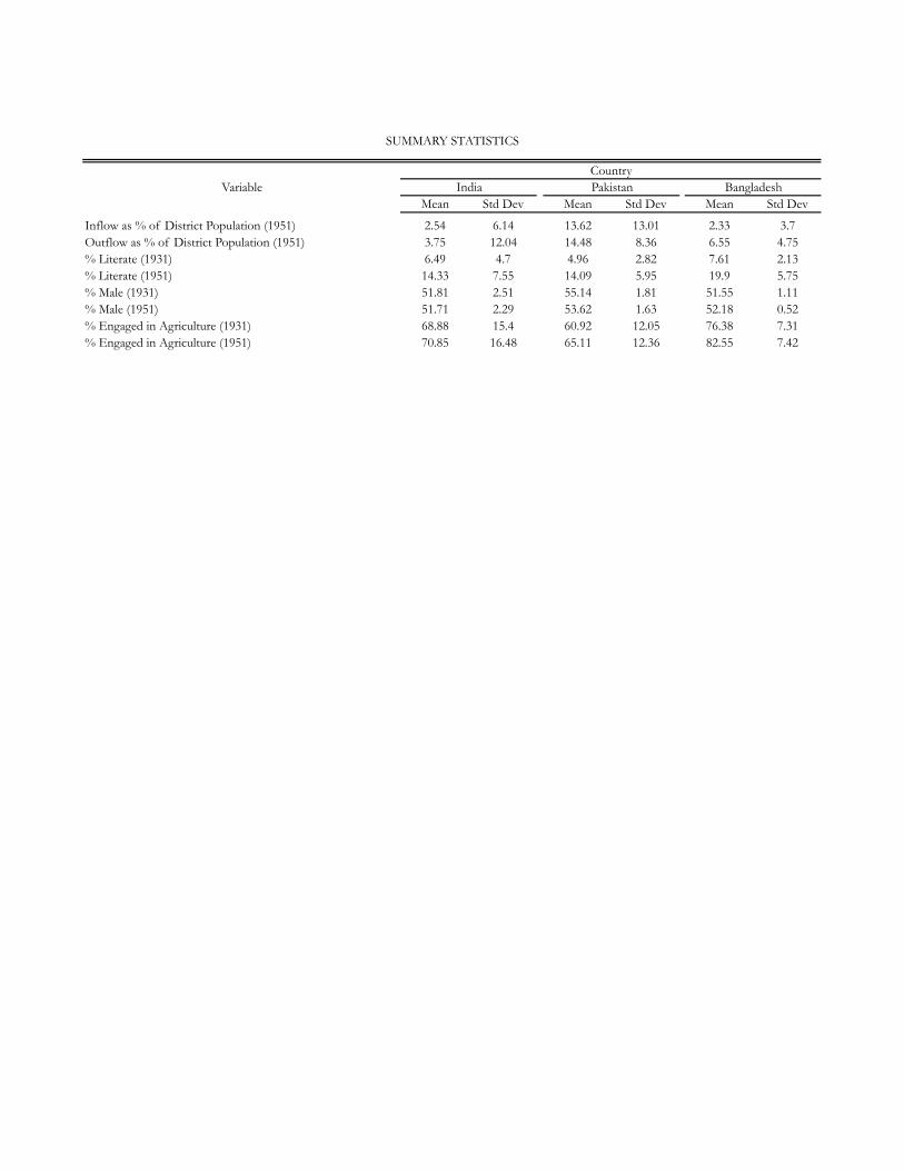
Inflow as % of District Population (1951) 2.54 6.14 13.62 13.01 2.33 3.7
Outflow as % of District Population (1951) 3.75 12.04 14.48 8.36 6.55 4.75
% Literate (1931) 6.49 4.7 4.96 2.82 7.61 2.13
% Literate (1951) 14.33 7.55 14.09 5.95 19.9 5.75
% Male (1931) 51.81 2.51 55.14 1.81 51.55 1.11
% Male (1951) 51.71 2.29 53.62 1.63 52.18 0.52
% Engaged in Agriculture (1931) 68.88 15.4 60.92 12.05 76.38 7.31
% Engaged in Agriculture (1951) 70.85 16.48 65.11 12.36 82.55 7.42
Variable
SUMMARY STATISTICS
Country
India Pakistan Bangladesh
Dependent Variable: Difference in Percent Literate (in District population) - 1951 minus 1931
(1) (2) (3) (4) (5) (6) (7) (8) (9)
Inflow as % of district population 0.15 0.16 0.041 0.063 -0.308 -0.093
[0.058]** [0.084]* [0.021]* [0.017]*** [0.253] [0.385]
Outflow as % of district population 0.048 -0.007 -0.089 -0.122 -0.245 -0.198
[0.028]* [0.040] [0.033]** [0.029]*** [0.168] [0.263]
Constant 4.36 5.64 4.309 0.405 1.085 0.378 6.173 5.944 6.274
[3.129] [3.094]* [3.150] [0.753] [0.672] [0.586] [3.568] [3.231]* [3.643]
Controls used
Observations 224 224 224 35 35 35 17 17 17
R-squared 0.52 0.51 0.52 0.97 0.97 0.98 0.65 0.67 0.67
B: difference in Resident literacy (1951-1931)
-----Basic + A----- -----Basic + B----- -----Basic + A-----
A: difference in Majority literacy (1931-1921)
Std Errors in brackets. * significant at 10%; ** significant at 5%, ***significant at 1%
This table examines the impact of inflows and outflows in a district on that district's percentage literate in 1951. Percent literate is defined in terms of the population.
Computation of outflow is discussed in the Appendix. Inflows are people moving into a given district due to partition, outflows are those moving out. The observations for India
are fewer than the usual 234 because we do not have 1921 information for 7 districts. We loose an additional 3 districts to outliers - these districts are Bombay (city), Cochin and
Muzzafarnagar. "Residents" in 1951 are just the people who did not move due to Partition. "Majority" is defined as Muslims in Pakistan/Bangladesh and Non-muslims in India.
Resident literacy (1951) cannot be computed for India as data on literacy of migrants was not collected.
TABLE I
IMPACT ON LITERACY AT DISTRICT LEVEL
India Pakistan Bangladesh
Basic controls: State fixed effects, percent Majority and Minority literacy in 1931, dummy for whether the district had a big city (defined in Bharadwaj, Khwaja & Mian 2008).

Dependent Variable: Difference in Percent Engaged in Agriculture (in District population) - 1951 minus 1931
(1) (2) (3) (4) (5) (6) (7) (8) (9)
Inflow as % of district population -0.363 -0.97 0.035 0.031 0.758 0.934
[0.231] [0.327]*** [0.135] [0.148] [1.060] [1.085]
Outflow as % of district population 0.068 0.398 0.042 0.023 -0.222 -0.265
[0.110] [0.154]** [0.262] [0.287] [0.276] [0.284]
Constant -19.74 -24.165 -17.824 6.487 6.773 2.545 5.315 8.939 5.787
[11.934] [11.837]** [11.749] [6.704] [7.964] [10.820] [5.415] [4.016]* [5.478]
Controls used
Observations 180 180 180 21 21 21 15 15 15
R-squared 0.39 0.38 0.41 0.87 0.87 0.87 0.18 0.19 0.26
Std Errors in brackets. * significant at 10%; ** significant at 5%, ***significant at 1%
This table examines the impact of inflows and outflows in a district on the % engaged in agriculture in that district in 1951. Computation of outflow is discussed in the Appendix.
Inflows are people moving into a given district due to partition, outflows are those moving out. Percent agriculture in India in 1951 includes dependents of the workers, while for
Pakistan & Bangladesh they are exluded. It is not possible to separate out dependents in the Indian figure, or include dependents in the Pakistani figure. In 1931 the % agriculture
figure includes dependents for India, but not for Pakistan and Bangladesh. Observations are fewer in these regressions as occupation data was collected only for some states in
1931. States included are Ajmer, Assam, Baluchistan, Bihar & Orissa, Bengal, Gwalior, Central India Agency, Hyderabad, Madhya Bharat, Madras, Mysore, NWFP, Punjab,
Rajputana, UP and Western Agencies. State fixed effects used in all regressions. "Residents" in 1951 are just the people who did not move due to Partition. "Majority" is defined as
Muslims in Pakistan/Bangladesh and Non-muslims in India.
TABLE II
IMPACT ON AGRICULTURAL OCCUPATION AT DISTRICT LEVEL
India Pakistan Bangladesh
A: difference in Majority literacy (1931-1921)
Basic controls: State fixed effects, percent Majority and Minority literacy in 1931, dummy for whether the district had a big city (defined in Bharadwaj, Khwaja & Mian 2008).
-----Basic + A----- -----Basic + A----- -----Basic + A-----

Dependent Variable: Difference in Percent Men (in District population) - 1951 minus 1931
(1) (2) (3) (4) (5) (6) (7) (8) (9)
Inflow as % of district population -0.026 -0.003 -0.017 -0.019 0.002 0.056
[0.014]* [0.020] [0.007]** [0.008]** [0.066] [0.093]
Outflow as % of district population -0.018 -0.017 -0.008 0.004 -0.029 -0.059
[0.007]** [0.010]* [0.010] [0.011] [0.049] [0.070]
Constant -0.094 -0.17 -0.15 0.71 0.811 0.936 -1.454 -1.194 -1.402
[0.791] [0.777] [0.788] [0.220]*** [0.258]*** [0.245]*** [0.927] [0.851] [0.942]
Controls used
Observations 227 227 227 35 35 35 17 17 17
R-squared 0.3 0.31 0.31 0.97 0.96 0.97 0.72 0.73 0.74
B: difference in % male among Residents (1951-1931)
Basic controls: State fixed effects, percent Majority and Minority literacy in 1931, dummy for whether the district had a big city (defined in Bharadwaj, Khwaja & Mian 2008).
-----Basic + A----- -----Basic + B----- -----Basic + A-----
Std Errors in brackets. * significant at 10%; ** significant at 5%, ***significant at 1%
This table examines the impact of inflows into and outflows from a given district on gender ratios in 1951. Computation of outflow is discussed in the Appendix. Inflows
are people moving into a given district due to partition, outflows are those moving out."Residents" in 1951 are just the people who did not move due to Partition. "Majority" is
defined as Muslims in Pakistan/Bangladesh and Non-muslims in India. The observations for India are fewer than the usual 234 because we do not have 1921 information
for 7 districts.
TABLE III
IMPACT ON GENDER AT DISTRICT LEVEL
India Pakistan Bangladesh
A: difference in % male among Majority population (1931-1921)
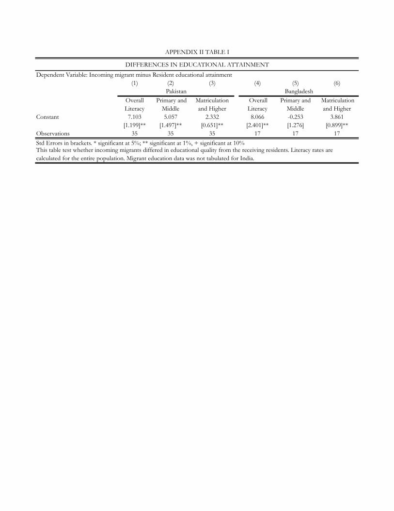
Dependent Variable: Incoming migrant minus Resident educational attainment
(1) (2) (3) (4) (5) (6)
Overall
Literacy
Primary and
Middle
Matriculation
and Higher
Overall
Literacy
Primary and
Middle
Matriculation
and Higher
Constant 7.103 5.057 2.332 8.066 -0.253 3.861
[1.199]** [1.497]** [0.651]** [2.401]** [1.276] [0.899]**
Observations 35 35 35 17 17 17
Std Errors in brackets. * significant at 5%; ** significant at 1%, + significant at 10%This table test whether incoming migrants differed in educational quality from the receiving residents. Literacy rates are
calculated for the entire population. Migrant education data was not tabulated for India.
APPENDIX II TABLE I
DIFFERENCES IN EDUCATIONAL ATTAINMENT
Pakistan Bangladesh

Dependent Variable: % Literate in Incoming Migrants
(1) (2) (3) (4)
Distance -0.238 -0.166 -0.457 1.14
[0.177] [0.130] [0.843] [1.145]
Distance Sq 0.001 0.001 0.007 -0.017
[0.001]+ [0.001] [0.013] [0.020]
District Outflow as % of
Total Outflow-0.555 0.059 -0.639 -0.435
[1.299] [0.569] [0.415] [0.366]
Minority-Majority ratio 1931 -0.368 0.1 0.411 0.395
[0.365] [0.220] [0.206]+ [0.211]+
% Literate in majority
population, 19310.694 -0.158 2.716 1.787
[1.128] [0.703] [1.038]* [1.064]
% Literate in minorities,
19310.908 0.739 1.689 0.618
[0.388]* [0.367]+ [0.501]** [0.747]
City Dummy 5.961 5.157 27.364 23.439
[11.594] [4.665] [6.386]** [6.939]**
Constant 29.621 17.05 -13.217 -16.784
[14.630]+ [8.755]+ [11.945] [15.387]
Observations 35 35 17 17
R-squared 0.57 0.52 0.88 0.9
Weights None Inflows None Inflows
Std Errors in brackets. * significant at 5%; ** significant at 1%, + significant at 10%
This table examines the impact of distance, outflow, minority-majority ratio, % literates
among majority and minority population and the presence of a city in the district on
the proportion of literates in the incoming migrant population in that district.
Computation of outflow is discussed in the Appendix. Inflows are people moving into
a given district due to partition, outflows are those moving out. Distance is measured as
the straight line to the border from the center of a district. Minorities in India are
Muslims. In Pakistan and Bangladesh minorities are Hindus and Sikhs. The remaining
population is the majority in each country. City dummy was created from the 24 largest
cities (in terms of population) from 1931. This data was obtained from the Historical
Atlas of South Asia (Schwartzberg, 1978). Migrant education was not tabulated for
India.
APPENDIX II TABLE II
WHERE DID LITERATES GO?
Pakistan Bangladesh
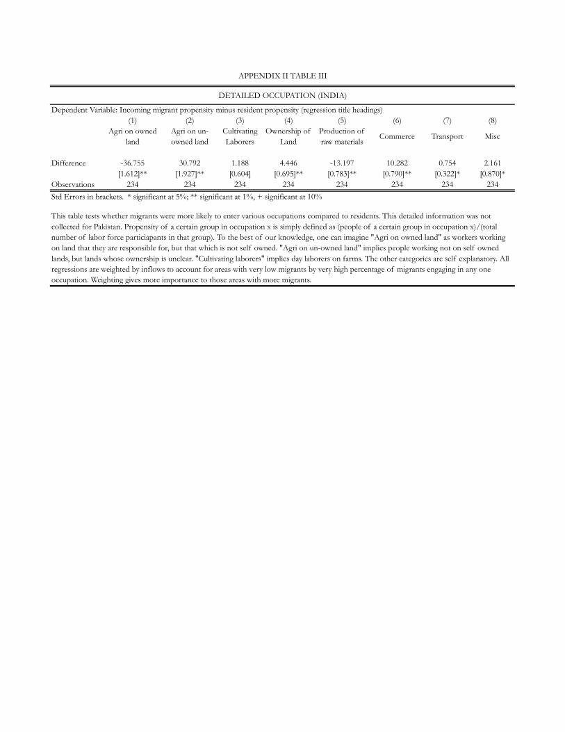
Dependent Variable: Incoming migrant propensity minus resident propensity (regression title headings)
(1) (2) (3) (4) (5) (6) (7) (8)
Agri on owned
land
Agri on un-
owned land
Cultivating
Laborers
Ownership of
Land
Production of
raw materialsCommerce Transport Misc
Difference -36.755 30.792 1.188 4.446 -13.197 10.282 0.754 2.161
[1.612]** [1.927]** [0.604] [0.695]** [0.783]** [0.790]** [0.322]* [0.870]*
Observations 234 234 234 234 234 234 234 234
APPENDIX II TABLE III
DETAILED OCCUPATION (INDIA)
Std Errors in brackets. * significant at 5%; ** significant at 1%, + significant at 10%
This table tests whether migrants were more likely to enter various occupations compared to residents. This detailed information was not
collected for Pakistan. Propensity of a certain group in occupation x is simply defined as (people of a certain group in occupation x)/(total
number of labor force particiapants in that group). To the best of our knowledge, one can imagine "Agri on owned land" as workers working
on land that they are responsible for, but that which is not self owned. "Agri on un-owned land" implies people working not on self owned
lands, but lands whose ownership is unclear. "Cultivating laborers" implies day laborers on farms. The other categories are self explanatory. All
regressions are weighted by inflows to account for areas with very low migrants by very high percentage of migrants engaging in any one
occupation. Weighting gives more importance to those areas with more migrants.
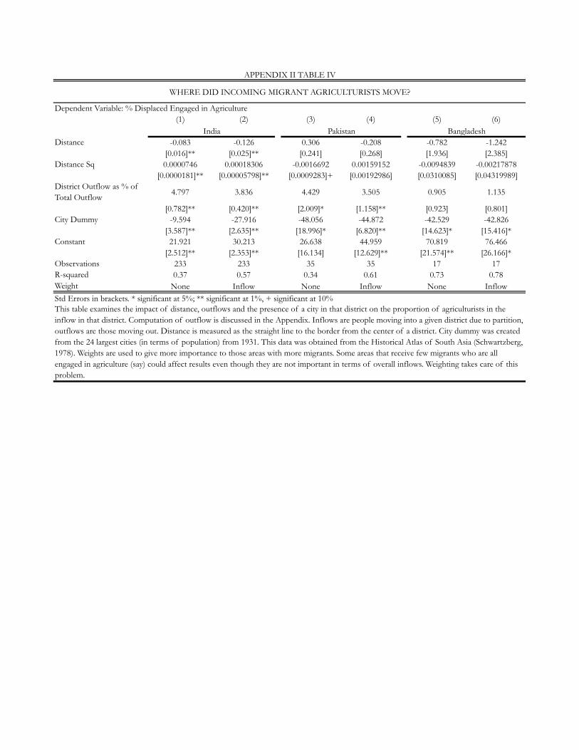
Dependent Variable: % Displaced Engaged in Agriculture
(1) (2) (3) (4) (5) (6)
Distance -0.083 -0.126 0.306 -0.208 -0.782 -1.242
[0.016]** [0.025]** [0.241] [0.268] [1.936] [2.385]
Distance Sq 0.0000746 0.00018306 -0.0016692 0.00159152 -0.0094839 -0.00217878
[0.0000181]** [0.00005798]** [0.0009283]+ [0.00192986] [0.0310085] [0.04319989]
District Outflow as % of
Total Outflow4.797 3.836 4.429 3.505 0.905 1.135
[0.782]** [0.420]** [2.009]* [1.158]** [0.923] [0.801]
City Dummy -9.594 -27.916 -48.056 -44.872 -42.529 -42.826
[3.587]** [2.635]** [18.996]* [6.820]** [14.623]* [15.416]*
Constant 21.921 30.213 26.638 44.959 70.819 76.466
[2.512]** [2.353]** [16.134] [12.629]** [21.574]** [26.166]*
Observations 233 233 35 35 17 17
R-squared 0.37 0.57 0.34 0.61 0.73 0.78
Weight None Inflow None Inflow None Inflow
Std Errors in brackets. * significant at 5%; ** significant at 1%, + significant at 10%
This table examines the impact of distance, outflows and the presence of a city in that district on the proportion of agriculturists in the
inflow in that district. Computation of outflow is discussed in the Appendix. Inflows are people moving into a given district due to partition,
outflows are those moving out. Distance is measured as the straight line to the border from the center of a district. City dummy was created
from the 24 largest cities (in terms of population) from 1931. This data was obtained from the Historical Atlas of South Asia (Schwartzberg,
1978). Weights are used to give more importance to those areas with more migrants. Some areas that receive few migrants who are all
engaged in agriculture (say) could affect results even though they are not important in terms of overall inflows. Weighting takes care of this
problem.
APPENDIX II TABLE IV
WHERE DID INCOMING MIGRANT AGRICULTURISTS MOVE?
India Pakistan Bangladesh
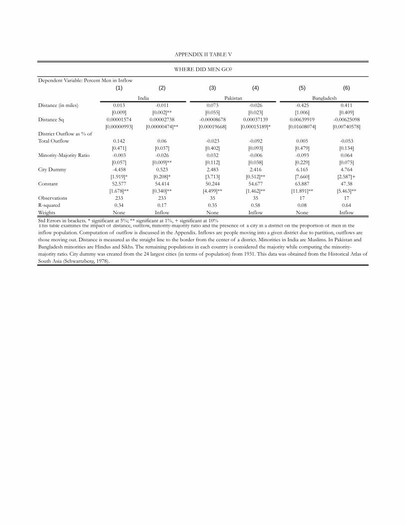
Dependent Variable: Percent Men in Inflow
(1) (2) (3) (4) (5) (6)
Distance (in miles) 0.013 -0.011 0.073 -0.026 -0.425 0.411
[0.009] [0.002]** [0.055] [0.023] [1.006] [0.409]
Distance Sq 0.00001574 0.00002738 -0.00008678 0.00037139 0.00639919 -0.00625098
[0.00000993] [0.00000474]** [0.00019668] [0.00015189]* [0.01608074] [0.00740578]
District Outflow as % of
Total Outflow 0.142 0.06 -0.023 -0.092 0.005 -0.053
[0.471] [0.037] [0.402] [0.093] [0.479] [0.134]
Minority-Majority Ratio -0.003 -0.026 0.032 -0.006 -0.093 0.064
[0.057] [0.009]** [0.112] [0.038] [0.229] [0.075]
City Dummy -4.458 0.523 2.483 2.416 6.165 4.764
[1.919]* [0.208]* [3.713] [0.512]** [7.660] [2.587]+
Constant 52.577 54.414 50.244 54.677 63.887 47.38
[1.678]** [0.340]** [4.499]** [1.462]** [11.891]** [5.463]**
Observations 233 233 35 35 17 17
R-squared 0.34 0.17 0.35 0.58 0.08 0.64
Weights None Inflow None Inflow None Inflow
Std Errors in brackets. * significant at 5%; ** significant at 1%, + significant at 10%This table examines the impact of distance, outflow, minority-majority ratio and the presence of a city in a district on the proportion of men in the
inflow population. Computation of outflow is discussed in the Appendix. Inflows are people moving into a given district due to partition, outflows are
those moving out. Distance is measured as the straight line to the border from the center of a district. Minorities in India are Muslims. In Pakistan and
Bangladesh minorities are Hindus and Sikhs. The remaining populations in each country is considered the majority while computing the minority-
majority ratio. City dummy was created from the 24 largest cities (in terms of population) from 1931. This data was obtained from the Historical Atlas of
South Asia (Schwartzberg, 1978).
APPENDIX II TABLE V
WHERE DID MEN GO?
India Pakistan Bangladesh