The Pareto-Lévy Law and the Distribution of Income · international economic reviewv may, 1 review ~~~~~vol. 1, no. 2 the pareto-levy law and the distribution of income* by benoit

Institute of Social and Economic Research, Osaka UniversityEconomics Department of the University of Pennsylvania

The Pareto-Lévy Law and the Distribution of IncomeAuthor(s): Benoit MandelbrotSource: International Economic Review, Vol. 1, No. 2 (May, 1960), pp. 79-106Published by: Wiley for the Economics Department of the University of Pennsylvania andInstitute of Social and Economic Research, Osaka UniversityStable URL: http://www.jstor.org/stable/2525289Accessed: 15-05-2016 23:08 UTC

Your use of the JSTOR archive indicates your acceptance of the Terms & Conditions of Use, available at

http://about.jstor.org/terms

JSTOR is a not-for-profit service that helps scholars, researchers, and students discover, use, and build upon a wide range of content in a trusted

digital archive. We use information technology and tools to increase productivity and facilitate new forms of scholarship. For more information about

JSTOR, please contact [email protected].

Wiley, Institute of Social and Economic Research, Osaka University, EconomicsDepartment of the University of Pennsylvania are collaborating with JSTOR to digitize, preserveand extend access to International Economic Review

This content downloaded from 132.239.66.164 on Sun, 15 May 2016 23:08:46 UTCAll use subject to http://about.jstor.org/terms

INTERNATIONAL

ECONOMIC

REVIEWV May, 1 REVIEW ~~~~~~~~~VOl. 1, NO. 2

THE PARETO-LEVY LAW AND THE DISTRIBUTION OF INCOME*

BY BENOIT MANDELBROT'

SUMMARY

THE PURPOSE of this paper is twofold. On the one hand, we wish

to give an account of a set of new models for certain distribution

properties of an important class of economic quantities, which includes

"income" (see [15], [17]). On the other hand, we think that the tools which we shall use are as important as the results which we hope to

achieve: that is, we intend to draw the economist's attention to the

great potentital importance of "stable non-Gaussian" probability dis-

tributions. To give a sharper focus to our paper, we shall develop our main points within the frame of a theory of income distribution;

but our approach will be immediately translatable in terms of similar

quantities, and our theory may well be more reasonable, or the em-

pirical fit better, in the case of some other quantities. We may thus

paraphrase what a famous author said of Brownian motion: it is possible that the properties which we shall study are identical to those of income;

however, the information available to us regarding incomes is so lacking in precision that we cannot really form a judgment on the matter.

This paper will be almost exclusively theoretical. Our point of de- parture will be an interesting empirical observation, namely, that over

a certain range of values of income U, its distribution is not markedly influenced either by the socio-economic structure of the community

under study, or by the definition chosen for "income." That is, these two elements may at most influence the values taken by certain param-

eters of an apparently universal distribution law. This law was dis- covered by V. Pareto in 1897 [24]; actually, several different statements

have at times been called "Pareto's law." In the introduction we shall

very carefully distinguish between these statements, and we shall comment upon some existing theories of income distribution.

* Manuscript received June 19, 1959. ' The work in this paper was started while the author was associated with the Uni-

versity of Geneva (under partial support of the Rockefeller Foundation), then with the University of Lille and the Ecole Polytechnique in Paris.

79


80 BENOIT MANDELBROT

We shall then introduce a new version of Pareto's law which be-

longs to the class of "stable" distributions, and which we shall designate as "the Pareto-Levy lawv" (P-L)c' This law also explains partially the data relative to the middle-income range.

The initial motivation for this law will be essentially twofold. First,

among all the possible interpolations of the weak (asymptotic) Pareto

law, the P-L law is the only one which strictly satisfies one (strong) form of the condition of invariance oi the distribution, relative to the

definition of income. Second, a P-L distribution is a possible linmit distribution of sums of random variables. That is, as we shall demon-

strate, the Gaussian distribution is not the only possible such limit (as is too generally assumed), and it is unnecessary (as well as insufficient) to try to save the limit argument by applying it to log U, instead of

U, as is done in some theories leading to the "log-normal law" for U. The P-L law turns out to have many other very desirable proper-

ties. it has also the drawback that it is limited to the interpolation

of Pareto's law, when its index a is such that 1 < a < 2, (see 1.1 for a definition of a).

In a series of other articles, which has started with [18], [19], [20], we also study the IP-L stochastic processes, a family of models of income variation. These processes agairn preserve certain desirable properties of the classical Gaussian processes without such drastic de- fects as the fact that income variation cannot possibly be Gaussian.

It turns out that in the high income range, a P-L Markovian process can be approximated by a randonm walk of log U: that is, we are able to derive the fundarnental initial assumptions of a model

due to Champernowne [2]. Moreover, a P-L Markovian process behaves quite reasonably in the intermediate range of incomes.

1. INTRODUCTION

1.1. The strong Pareto law. Let us begin with a basic variant, which will be referred to as the strong Pareto law. Let P(u) be the percentage of individuals with an income U (over some fixed period of reference) exceeding some number u (u is assumed to be a conr- tinuous variable). The strong Pareto law asserts that:

((u/?u)-, when u > u0

1P when u < u.

n This associates Pareto's name with that of Paul Levy, who first studied the stable distributions intensively. (See in particular Levy [10], [11], [12].) To the best of our knowl- edge the application of these laws to economics is entirely new as well as are the definition

and properties of the "Pareto-Levy" processes of [18), [19), [20).


THE PARETO-LEVY LAW 81

Then, the "density" p(u) = - dP(u)/du satisfies

I a(u 0)u-(a+l when u > u?

O(U) = 0 when u < ul. This distribution is fully specified by two "state variables": u0, a scale factor, and a, which will turn out to be some kind of index of inequality of distribution. The strong law leaves the value of a undeter-

mined (although in some cases, one immediately states that a > 1). We may also find the stronger statement that a -_ 3/2: the corresponding variant of the strong law will be referred to as the strongest Pareto

law. Graphically, the strong law implies that the ("double logarithmic") graph of y log P, as a function of v -log t, is a straight line.

The empirically observed P(u) are of course percentages relative to finite populations. They will further be considered as frequencies relative to a random sample, drawn from an infinite population. [Em- pirically, the law holds as well for samples of a few hundred (the

"burghers" of a city-state of the Renaissance) or of close to a hundred

million (the taxpayers in the USA).] That is, U will be treated as a random variable with values u, and the curve describing the variation of U in timne will be treated as a random function.

1.2. The weak Pareto law. The strongest Pareto law is now acknowledged to be empirically unjustified (and it should be noted that many purported "disproofs" of "the" Pareto law apply to this variant only). On the contrary, there is little question of the validity of the Pareto law ifi "sufficiently" large values of u are concerned. The best way of taking care of the limitations of the strong law is simply to state that:

P(u) "behaves like" (u/u0)? as U -- oo

This is the weak Pareto law. Such a statement is useful only if the exact definition of "behaves like" conforms to the empirical evidence and (taking advantage of the indeterminacy of such evidence) lends itself to easy mathematical manipulation. The following definition of "behaves like" is usually found to be adequate:

P(lu), (u/u? Mo That is:

P() -1, as u oo (uIuo)}0

or,

P(u) = {1 + e(u)}(u/u')0, where e(u) - 0, as u oo



Graphically, this means that the curve (log P, log u) is asymptotic to

the straight line which represents the strong Pareto law.

1.3. Interpolation of the weak Pareto law. The range of values of u which is accounted for by Pareto's analytic expression cove:s

only a part of the total population. Elsewhere the "density" -dP(u)/du is represented by a quite irregular curve, the shape of which depends

in particular upon the breadth of coverage of the data considered. This has been particularly clearly emphasized by H. P. Miller [22]. He has shown that the income distribution is skewed and presents

several maxima, if one includes all individuals, even those with no income and part-time workers, and if one combines the incomes of men and women. However, the separate income distributions oI most of the different occupational categories, as distinguished by the census,

are both regular and fairly symmetric; the main source of skewness in the overall distribution and hence in Pareto's law can be traced to

the inclusion of self-employed persons and managers together with all wage earners. One may also note that the method of reporting in-

come differs by occupational categories, and that, as a result, the cor-

responding data are not equally reliable.

The above reasons make it unlikely that a single theory could ever

explain all the features of the income distribution or that a single

empirical formula could ever represent all the data. As a result, it

has been frequently suggested that several different models may be required to explain the empirical P(u); unfortunately, we know of no

empirical check of this conjecture. In any case, the present paper

will be devoted almost exclusively to a theory of high income data

and of the weak Pareto law. It is unlikely that the interpolation of

the results of our model will be able to explain finally all the middle

income data. However, we shall not examine this point in great

detail.

1.4. Two laws of income distribution which are in contradiction with the weak Pareto law.

A. Pareto himself has suggested the following possible improvement

in his law:

p(u) = - dP/du - ku-0'4+1exp(- bu) (where b > 0)e

However, the weak Pareto law must be at least approximately correct for large u. Hence, the parameter b must be very small, and

the evidence against the hypothesis that b 0 is not strong. The

choice, therefore, between the hypotheses b = 0 and b # 0 may be legitimately influenced by ease of mathematical manipulation and ex-


THE PARETO-LtVY LAW 83

planation. We shall see that the weak Pareto law (b = 0) has some

crucial properties, which wsTill be used as a basis for a theory, and

which disappear if b / 0. We shall therefore disregard the case b t 0 (the more so since the formula 'above provides no improvement for middle values of ut). (See 2.4 for a further discussion of b = 0.)

B. The best known statement about income distribution, apart from

the weak Pareto law, is the log-normal law [8], [1], which claims that the variable log U [or perhaps better log (U-u'), where u'>0] is well

represented by the Gaussian distribution. The empirical evidence for

this is that the graph of (P, u) on log-normal paper seems to be straight. Such a graph emphasizes a different range of values of u from that of the Pareto graph, so that the graphical evidence for the two laws is not contradictory. The motivation for the log-normal law is, how-

ever, largely theoretical (see 1.5). Roughly speaking, a log-normal U can be explained by assuming that log U is the sum of many additive components.

1.5. Some existing models of income distribution considered as "thermodynamic" theories. There is a great temptation to consider the exchanges of money which occur in economic interaction as analo-

gous to the exchanges of energy which occur in physical shocks between gas molecules. In the loosest possible terms, both kinds of interactions 6"should" lead to "similar" states of equilibrium. That is, one "should" be able to explain the law of income distribution by a model similar to that used in statistical thermodynamics: many authors have done so explicitly, and all the others of whom we know have done so im-

plicitly.

Unfortunately, the Pareto P(u) decreases much more slowly than

any of the usual laws of physics, so that if one wants to apply the physical theory mechanically, one must somehow argud that U is a less intrinsic variable than some slowly increasing function V(U). For that, one must renounce the additive properties of U. The seemingly universal choice for V is V = log U [or V' r log (U - u')]. This choice is suggested by the fact that one plots log<u empirically. But it can also be traced back to the "moral wealth" of Berpouilli, and it apparently can be justified by some law of proportionate effect, or by some kind of Weber-Fechner law. If this choice of V is granted, one has to explain the normal law for the middle zone of v's, and the exponential law P(v) = exp {- a(v - v0)} for the upper zone of v's.

Indeed, many existing models of the Pareto distribution are reducible to the observation that (for any a) exp (- av) is a possible bar- ometric density distribution in the atmosphere. Alternatively, con-



sider a set of Brownian particles, floating in a gas at a uniform

temperature and density, the whole being enclosed in a semi-infinite

tube with a closed bottom and an open top; assume further that the

field of gravity is uniform. Then the density distribution which the

Brownian particles attain as a state of final equilibrium is the ex-

ponential. This is the result of a compromise between two forces, both uniform along the tube, i.e., the force of gravity, which alone would tend to pull all particles to the bottom, and the influence of heat

motion, which alone would tend to diffuse them all to infinity. Clearly, the models of income distribution we are now considering involve an

interpretation of the forces of diffusion and of gravity.

Unfortunately, such interpretations are never sufficiently intuitive to exclude, for example, the removal of the counterpart of the bottom of the tube. The trouble is that such a removal changes every-

thing. In fact, there is no steady limit state any longer, because all

the Brownian particles diffuse to ininus infinity. It is true that the

Gaussian distribution does appear as a conditional distribution for V

(this distribution is valid if one assumes that all the particles start from the same point), but this cannot really be a basis for a model

of the log-normal law.

This difficulty is already very clear in the simplest model of a diffusion, the so-called random walk, in which both time and V are quantified. Time is integral and V is a multiple of a unit v". This model (apparently introduced into economics by Champernowne [2]) fur-

ther assumes (1) that the variation of V is Markovian, that is, V(t+1)

is a function only of V(t) and of chance, and (2) that the probability

that V(t + 1) - v(t) = kv'" becomes independent of v(t) as v increases. Additional assumptions are required to get either Pareto's law or the

log-normal law, and the difference between these additional assump-

tions has no intuitive meaning, which makes both conclusions uncon-

vincing. However, the models which lead to the exponential are still

slightly better: in fact, we can, perhaps, argue that the apparent

normality of the "density" p(v) in the central zone of v's simply

means that - logp(v) may be represented by a parabola in that zone, whereas for large v's, it is represented by a straight line. Such a parabolic interpolation needs no limit theorems of probability for its

justification; it applies to any regularly concave curve, at least in the first approximation.

In the case of models of the weak Pareto law, further non-intuitive

assumptions are necessary to rationalize the empirical fact that a > 1 in all cases.



We shall not analyze any of the other existing translations into

economic terms of various models of the normal or exponential distri-

butions, which occur in statistical thermodynamics, such as gas equilibrium or Brownian motion. Because of their common "thermodynamic"

character, these theories are essentially equivalent. In particular, they do not assume any institutional income structure; all income re-

cipients are treated as entrepreneurs. A rewording of the classical

theories, however, can make them applicable to many possible institu-

tional structures of wage and salary earners; see Lydall [13]3.

In this article (see also [18]) we shall attempt to show that the

analogy of statistical physics need not be abandoned, if we want to

avoid the weaknesses which mar existing theories. We shall not re-

quire the transformnation V log U, and we shall not try to justify

the introduction of the economic counterparts of such conditions as

the presence or the absence of a bottom to the tube in which Brownian

motion is studied. That is, we shall not try to force income into the

structure of statistical thermodynamics (even implicitly); rather, we

shall attempt explicitly to generalize the statistical methods of thermo-

dynamics, in order to cover the economic concept of income.

We shall be successful only in the case where 1 < a < 2, a restriction which we shall discuss repeatedly.

2. PARETO-LEVY RANDOM VARIABLES

2.1. An analysis of the definition of income. One of the principal claims of this paper is that it is impossible to "explain" why Pareto's law, and not some other law, is satisfied by income distributions, with-

out also studying the inseparable problem raised by the fact that

essentially the same law continues to be Jollowed by the distribution Of "income," despite changes in the def,inition of this term. Such an invariance is of course very important to census analyzers, because

of the small effect of large changes in methods of estimating income. To study this problem one needs a practical way of expressing the different definitions of U. We shall argue that there are several ways of distinguishing different sources of U. Therefore, U may be written in different ways as a sum of elements, such as: A, agricult-

3 We had indenpendently rediscovered this model and had discussed it in the original text of this paper, as submitted on June 19, 1959. The coincidence of the predictions of the P-L model and of the Lydall model for 1<a <2, shows that the distribution which corresponds to the least amount of organization could be "frozen" without modi- fying it, reinterpreted as a wage distribution and then let to evolve along conceptually quite different lines. This fact has great relevance to the problem of the value of a and to the fact that a has recently tended to increase beyond 2, in highly organized industrial societies.



ural, commercial, or industrial incomes; B, incomes in cash or in kind;

C, ordinary taxable income or capital gains; D, incomes of different members of a single taxDaying unit, etc... Let the -income categories

in a certain decomposition of U be labeled as Us (1 ? i <1 N). We shall assume that every method of reporting or estimating income corre-

sponds to the observation of the sum of the U, corresponding to some subset of indices i. This quite reasonable consideration imposes the

restriction that the scale of incomes themselves is more intrinsic than

any transformed variables, such as log U.'

Let the incomes in the categories U, be considered as statistically independent. This assumption idealizes the actual situation. A priori,

this abstraction may seem a bad first approximation, since when in-

come is divided into two categories U' and U", such as agricultural and industrial incomes, the observed values u' and u" are usually very

different. We shall find, however, that in the weak Pareto case, when the parts are independent, one would actually expect them to be very unequal; bence, although such an inequality cannot be a confirmation of independence, at least it does not contradict it in this case.

Under these assumptions, the only probability law for income which could possibly be observed must be such that if U' and U" follow

this law (up to a scale transformation, and up to the choice of origin),

then U' E U" must also follow the same law (the sign 0D designates the addition of random variables). That is, whatever a'>O, b', a">O, b", there exist two constants a > 0 and b, such that

(a'U + b') 0D (a"U + b") = aU + b.

Such a probability law is said to be "stable" (under addition), and its density as well as the variable U itself are "stable." The family

of all laws which satisfy this requirement has been constructed by Paul Levy [10]: it includes, naturally, the Gaussian law, but it also includes certain non-Gaussian laws, each of which turns out to satisfy the weak Pareto law, with some 0 < a < 2. In other words, the addi- tivity property of U, and the behavior of P(u), under the weak Pareto law (both of which disappear if the scale of U is changed) turn out

to be precisely sufficient and necessary for the application of Le'vy's theory of stable laws.

Further, the parameters of a non-Gaussian stable law can be ar-

ranged so that E(U) < co, which requires 1 < a < 2, and so that

p(- u) decreases very much faster than p(u), when u o oo: in the

I The same kind of division may also be performed in the direction of time. The problem arises that it is unlikely that the year be an intrinsic unit of time. If it is not, how can a single law hold irrespective of the time unit chosen? See [181, [191, [291.


THE PARETO-LtVY LAW 87

latter case, the stable law may be called positive, an abbreviation for

"gmaximally skewed in the positive direction."

Since the usual terminology of probability (stable distributions) does not serve our purpose, we propose to refer to "positive" stable distributions with 1 < a < 2, as "Pareto-Levy distributions."

It is not strictly true that the distribution of income is invariant

over the whole range of u, with respect to a change in definition of income. We argue, however, that if the variable U is not Gaussian and is very skewed, the most reasonable "first order" assumption about income is that it is a P-L variable.

The density p(u) of the P-L law unfortunately cannot be expressed

in a closed analytic formi, but is determined by its bilateral Laplace transform (valid for b > 0):

G(b) - exp bu) I dP(u) 5 exp ( bu)p(u)du = exp {(bu*)&' + Mb},

which depends upon three parameters: a (1 < a < 2), u* (which is a positive scale parameter), a-nd 111 (which is identical to E(U)).

G(b) yields the result:

P(u) - uO[u'F(1 - a)]O for u cX

where F(1 - a) is the Euler gamma-function.

For other values of u, the Pareto-Levy distribution had to be computed. A few sample graphs of densities appear in Figure 1. More

detailed tables will be published by Mandelbrot and Zarufaller [21]. We see that as long as a is not close to 2, the P-L density curve

very rapidly becomes indistinguishable from a strong Pareto curve of the same a. [For this, the origin of the strong Pareto curve must

be chosen properly and one must have u uX*F(1 - a).] The two curves converge n-ear u = E(U), when a is in the neighborhood of 3/2, and at even smaller values of u, when a is less than 3/2: that is, the asymptotic behavior of P(u), derived from G(b), is very rapidly im- plemented. As for large negative values of u, by the P-L law they

have a probability which is not zero, but decreases so rapidly as ui co,

that they may be safely disregarded; one finds that

log log p(u)]>- a log I uI e a- 1

This is a faster decrease than in the case of the Gaussian density- see Appendix I.



+

02

I L (D~~~~~~~

0 00 0 0 0 00 0o Il O D 49 CV O 0 qD t N ? @ eP ? C

N CJ C4 C4 clJ (n)d ?

_+- N~~~~~

5 2 0 0 O 0

+

0

0Q (D C\ N N Q O, 0.O

(n) d

4 z N

+

0

+ _ n

+

+0

N

CQ NQ Q o

I I l I I I I I I I 0 0 0 ( I

CD C D CNJ 0O 0 e C\J O CD eD v N O

(n) d



Finally, near E(U) and the most likely value of U, the P--L curve has the kind of skewness which one finds in the empirical data and which one hopes to derive in a theoretical curve.

Let a now approach 2. At the limit, the P-L density will tend toward a Gaussian density. Close to the limit, the P-L density already resembles a Gaussian one. Only for large values of u, (which have a very small probability) is the Gaussian decrease of P(u) replaced by a Paretian decrease.

In other terms, the P-L density is worth considering only if a is not "too close" to 2. Even in this range, however, the prediction for intermediate values of u is quite inadequate to cover the complete curve of incomes, as described for example by Miller [22]. But as part-time and unskilled workers are eliminated we more nearly approximate such a curve. On the other hand, the income distribution of unskilled workers is fairly symmetric and has a fairly small dispersion.' Since the distribution of unskilled wages differs from that of high incomes, the P-L law would a priori explain only the latter incomes. If we examine any income category as defined by the Bureau of Census, we can seldom tell in advance whether its income mechanism is closer to that of the unskilled workers or to that of the largest income re- cipients. Therefore, if we wish to determine how wide are the categories to which the P-L law applies, the only solution is to start from the P-L interpolation of high incomes, and then to see how many other incomes (and which) must be added to obtain a good fit. This establishes a distinction between two kinds of income categories. The reasonableness of this distinction should be checked on independent grounds. For the time being we shall be content to observe that for a far enough from 2 the prediction made by the P-L law is "reasonable." (cf. 2.6.)

We shall conclude this section with a few statements concerning non-P-L stable distributions. The Gaussian distribution is of course stable, and it is the only stable distribution with a finite variance. Further, all the stable variables with a finite mean are differences of P-L variables scaled by arbitrary positive coefficients. The bilateral generating function is no longer defined, and we must consider the usual characteristic function (cof.). For a P-L variable, the c.f. is immediately obtained as

9D(?)=3 _ e1"p(u)du = exp[-iM - _'I (ut)*{1 i' tg.53r}cos aj.

6 We may even think that their incomes would become non-random if their occupations were entirely interchangeable and if their changes in type of employment were without obstruction and costless.



Hence, denoting by (1 + e)/(1 - ) the ratio of the positive and negative components, the general stable variable, with E(U) < co, has a c.f. of the form:

= exp[- iMC - Kl(u*)W{1 - tg t7r }cos t]

where u> ?0, 1,8I < I and 1 < a < 2. (We may note that the same formula, with 0 < a < 1, gives another

family of stable variables, with E( U) = oo. The stable variables which do not fall into either of the above families are those of Gauss and

of Cauchy and finally a small family of variables connected with those

of Cauchy.)

2.2. Another (equivalent) property of the stable laws. The stable

laws have another (equivalent) property: they are the only possible

limit laws of weighted sums of identical and independent random

variables.8 That is, if U is decomposed into a sum of a large number

of components Us, we need not resort to the above argument of ob-

servational invariance; we know that (1) if the sum is not Gaussian (which is a conspicuous fact), (2) if the expected value of the sum is

finite (which is also a fact), and (3) if the probability of -u is much less than that of u, for u > 0 and large, then no hypothesis about the

distribution of the parts is necessary to conclude that the sum can only be a Pareto-Levy variable. We shall develop these points in

more detail, and in 2.6 we shall show that the above restrictions may

be reduced to broad "qualitative" properties, such as 'the likelihood that two independent variables U' and U" contribute unequally to the sum U' 6f U".

B Every stable law is such a limit. To prove this, assume that the variables Us them-

selves are stable; by induction of stability, the e-sum v 1 U8 will be a variable of the form a(N)U + b(N) and hence {a(N)I-I{(ZfN1Ui) - b(N)} will have the same distribution function as U. Conversely, assume that a certain normed sum of the variables

Ui has a limit. Write the N-th normed sum, taken in the sense of E, as:

N

A(N) Us - B(N) S-1

;A() .A(n) U- B(n)- A( A(m) - +C(N(m) Q )

where N = n + m. By letting both n and m tend to infinity, we find that the definition

of a stable variable must be satisfied by the limit of A(N)Zt..lUL - B(N) + C(N). We should also mention the following theorem of Gnedenko. For the convergence of

N' Y i -1Ui - B(N) to a stable limit, it is necessary and sufficient that 0 < a < 2, and that for u > 0, F(u) - 1 - P(u) 1 - {1 T e'(u)j(u/ul)-, where e'(u) -O 0, as u e, and for u < 0, F(u) {1 + eff(u)1(u/u2)w, where e"(u) -O 0, as u - oo.


THE PARETO-LE VY LAW 91

It should be noted that an explanation of the distribution of income in terms of the addition of many contributions does not involve the

log U transformation. This avoids the usual limit argument, which

leads to the log-normal law and contradicts Pareto's law.

These results may be better than expected because the limit distribu-

tion might not hold for U, which is a sum of only a few random com-

ponents. That is, if one wants to increase the number of components

of U, one must abandon the hypothesis of independence at some point:

the more U is subdivided the less independent the components become.

This is a difficulty which is not proper to the problem of income, but is acutely present in all social science applications of probability theory.7

Of course, the principle of the difficulty appears in physics for example in explaining why some kind of noise is Gaussian. But in most physi-

cal problems there exists a sufficiently large zone between the systems which are so small that they are impossible to subdivide and those which are so large that they can no longer be considered as homogeneous. No such zone exists in most problems of economics, so that a seemingly successful application of a limit theorem may seem too good to be true.

To sum up, it cannot be strictly true that the additive components

are indepenident and hiave the same distribution (up to scale). However, the "likelihood" of any distribution is greatly increased if this is the only one reducible to limit arguments. Hence, if a sum of many co,mponents is not Gaussian, is skewed, and such that E(U) < o, then the most reasonable first assumiption concerning the sum is that it follows the Pareto-Levy law.

More precisely, two extreme interpretations are possible. The "mini-

mal" interpretation regards the Pareto-Levy distribution as just another law which is correct asymptotically, is sutfficiently easy to handle, and is useful in the first approximation (after all, the Gaussian it-

self is frequently a good first approximation to distributions which, actually, are certainly not Gaussian).

At the other extreme we may take the Pareto-Le6vy law entirely seriously, and try to check its ability to predict some properties of income distribution which otherwise would seem independent of the weak Pareto law. We think that sucih predictions were in fact achieved. This provides some claim for a "maximal" interpretation of the P-L

law, which regards its invariance and limit properties as being "ex- plicative. "

2.3. Stable laws are very well known in abstract probability theory

In estimating a mean by an empirical average, often the sample is too small or the

many available data are strongly correlated.



(cf. Le6vy [10], [111, [12], Gnedenko and Kolmogoroff [8]). We might, therefore, have introduced the P-L law without special motivatior other than the fact that the known asymptotic behavior of P(u) and its recently computed behavior for intermediate u make it an attrac-

tive interpolation for the income data (Mandelbrot [18]). Unfortunately, the behavior of tlle P-L law is in many other ways quite different from that to which most statisticians are accustomed from their con-

stant handling of the Gaussian law. The only way of really showing how far this law is suited to the present problem is to sketch its

theory, starting with a heuristic introduction to its properties (from the viewpoint of addition and of the study of extremal values), and ending with some rigorous results.

We see how the three main drawbacks of the classical theories

vanish. Many variants of the same argument ali lead to the same result; no change of scale of U is necessary, the behavior of P(u) being exactly what is needed, and a is "near" 3/2. In fact, a should not be too close to 2, and cannot be greater than 2, a point which requires some elaboration.

2.4. Concerning the sign of a -2 and the variance of U. A few empirical data claim to lead to a > 2. To explain this by a limit argument requires most specific and unlikely assumptions. Similarly, the observational invariance of the stable distribution cannot hold if a > 2, unless it is weakened (2.5) to require that the sum of a few weak Pareto variables with a > 2 is a weak Pareto variable with a > 2; as the number of addends increase (2.8), the weak Pareto law holds for

a decreasing zone of values of u and finally the sum tends towards a Gaussian variable.

We find that the sign of a - 2 distinguishes two sets of different

random variables. The occurrence of a > 2, or even a < 2 but close to 2, may mean a predominance of salaries (Lydall's income model [13] is valid for all values of a). (Another explanation may be found in Mandelbrot [19].) On the other hand, several of the examples where a > 2 are encountered occur in communities of Oceania which are very much less self-contained than, for example, Great Britain or the

U.S.A. Their distributions of U may perhaps be truncated. In any case, the sign of a - 2 raises an important empirical problem: Is the fit of the weak law equally good regardless of this sign, and does this

law represent a higher percentage of the data where a < 2 ? A second consequence of the limitation 1 < a < 2 is that the second

moment of U is then infinite, the first moment being finite. This is

easily seen, because by integration by parts,



E(U) udF(u) - y tdPut) | P(u)du < X _ 0 , 0 0 0o

and D(U) = E(U2) - [E(U)]2 where

E(U2) u2d.F(u) = u'dP(u) = 2 uP(u)du = co

(We assume that the behavior of P(u) for negative u does not lead

to a convergence problem for E(U).)

The last result holds for both strong and weak Pareto variables if

1 < a < 2, but it would, for example, cease to hold for the density

p(u) = ku-10`'1 exp(- bu) of 1.4. This provides a new and important test of our conjecture that b =_ 0. The finite E(U) means that if u, are samples from a Pareto distribution, the empirical mean E, Et- Us/N tends to E( U) with probability 1 (Kolmogoroff's strong law of large numbers); in addition, EN is a good estimate for E(U), if N

is large. Now consider DN = E'- (u, - EN)21N. If a> 2, DN tends to a finite limit D( U), of which it is a good estimate, and E '-, (u, -E) tends to a Gaussian variable. This result changes little if one adds an

exponential factor with small b. However, if a < 2, and b 0 the lirnit of DN is infinity (one may show that D, grows without limit like N2'-1) but if b becomes > 0, D(U) is finite. Therefore, the use-

fulness of the exponential factor exp(- bu) may be tested by check-

ing whether DN keeps increasing with N in the case of the largest of the samples available. We could not make the direct test, but an

indirect test results from the following observation: the ordering of

the different populations by "increasing inequality" should presumably be identical with their ordering- by decreasing a; on the other hand,

more usual measures of inequality are given by Dy, DN/EN or VDK14EN. These two methods of ordering populations have been compared and found entirely contradictory. This result ceases to be absurd if one takes account of the fact that the values of N in the different samples which were compared range from 102 to 108; and it seems that even if D(U) were finite, it would not be approached, even with the largest samples. In that case, irrespective of any theory, it is pref-

erable to take b = 0, and D(U) = co. Further, Ino function of DN is adequate to compare degrees of inequality, except perhaps between samples of identical size.

Another test of the usefulness of the approximation D = co is pro-

vided by the relative contribution to DN of the largest of the u,: this is very large (close to 1/2 for the Wisconsin incomes [23]), as might be predicted from the theory of the Pareto-Levy law. The usual procedure



of truncating U in order to avoid D = co distorts the whole problem. 2.5. Heuristic study of the addition of tvo independent random

variables, particularly in the Gaussian and weak Pareto cases. Let

U' and U" be two independent random variables, having the same probability density p(u). We shall compare the behavior of p(u) for

large u, and that of p2(u) | p(x)p(u - x)dx, which is the density

of the sum U = U'QD U". It will be assumed that u may vary to + co.

One basic case is

p(u') = C exp(- bu') if u' > 0, 0 if u' <0.

Then,

p2(u) = C2exp(-bx)exp[-b(u-x)ldx 0

= C exp(- bu)dx = C2u exp(- bu).

Note that in this case log[p(u')] = logC-btb' is represented by a straight line. The two next simplest cases are those where -log [p(u')]

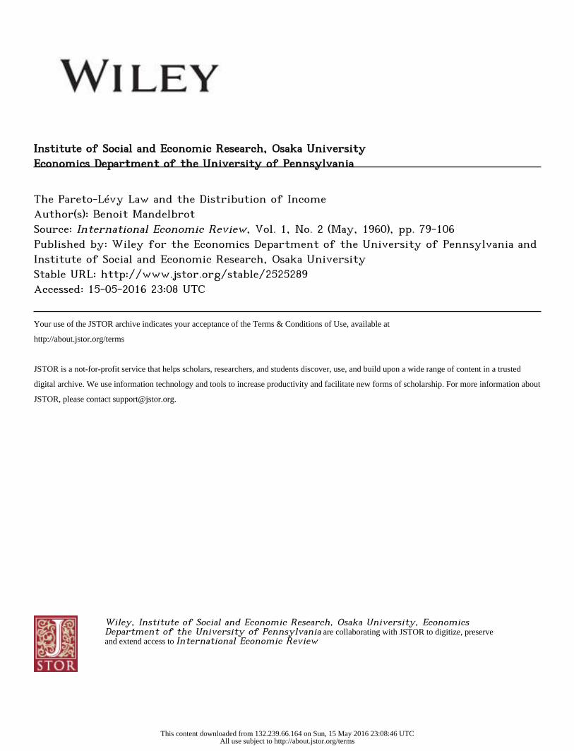
has the same convexity, up or down, over the whole range of variation of u', so that the expression - log p(x) - log p(u - x) has an ex- tremum for x = u/2. These two cases are illustrated in Figure 2.

One kind of convexity arises when d2 logp(u)/du2 < 0, for all u. Then p(u) decreases rapidly as u - co, and the integrand p(x)p(u - x)

has a maximum for x = u/2. If that maximum is strong enough, the

integral } p(x)p(u - x)dx is likely to be made up to a great extent

of the contributions of the x's in a small interval near u/2. Hence,

a large value of u is likely to come from two contributions u' and u" which are almost equal. (This is not obvious, and in particular it is not true if the concavity of -log p is turned the other way.)

Consider for example the Gaussian density

P(X)= e exp 2x

It is known that

P2(U) =exp

so that the Gaussian character of density is preserved in addition, except for the value of a. The same result can also be obtained heu-


THE PARETO-LVYY LAW 95

ristically, by arguing that p(x)p(u - x) stays near its maximum value

(u/2W}2 over some interval D/2 on each side of u/2, and is negligible elsewhere. In that case, one gets the approximate estimate:

p2(A) - p(uf2)p(u/2)D - exp (-. 4)>

In other words, the approximate estimate is correct, if one takes D a/i/ independent of u.

Suppose now that p(u) decreases slowly, so that d' log p(u)/du2 > 0, for all u. Then p(x)p(u - x) has a minimum for x = u/2. It may

I

Ul~~~~~~~~~

U U

U U 'a '~~~~~~~2

0 0 _~~~~~~~4

p (U 1) p (U/

FIGURE 2: DISTRIBUTION OF U' WHEN U'G U" IS KNOWN

be noted that p(x) must - 0 as x -- co and must either = 0 or 0 as x -. - co. This is compatible with a - log p(x) concave downwards, but only if the range of variation of x is truncated froin below. As-



sume that u' can only be 2 u?, so that its most probable value is u0. In that case, p(x)p(u - x) will have two maxima, for x = u? and for

x = u - u?. If they are strong enough, p2(zt) will be composed mostly of the contributiorns of the neighborhoods of these maxirmla. Compare then the following two expressions:

p2(u) = 2 p(x)p(u - x)dx, and 2 p(x)p(u)dxo o o

These two expressions differ only in the small contributions of x's very different from x - 0; that is,

p2(u) A 2p(u) p(x)dx 0

Finally, if u is large, p(x)dx p(x)dx, so that o O

p,(u) 2 p(u)e

Hence,

p2(x)dx = P,(u) 2P(u).

Note that a large valze of u is now likely to be the sum of a relatively very small value of either u' (or u") and of a value of u" (or u') very close to u - u'. The two addends are likely to be of very unequal size; but the problem is entirely symmetric, so that the mean value E(u'/u) is still u/2, by compensation. (See also Appendix II.)

We have in addition proved that the distribution of the largest of two variables U' and U" of the slowly decreasing type has the same asymptotic behavior as the distribution of their sum. Another derivation of this result starts from the derivation of the distribution of

max((U', U"). Clearly, Pm(u), the probability that u be larger than max(U', U") is the probability that ut be larger than both u' and u". Hence,

I - Pm(u) = [1 - P(u)]2.

For large u and small P(u), this becomes

Pm(u) ~ 2P(u) .

That is, for slowly decreasing densities, Pm(u) P,(u). A prototype of the slowly decreasing variable is the strong Pareto

variable. In that case, we can write:

P2(u) ~ 2P(u) = P(2'0 u).



That is, the sum of two independent and idential strong Pareto variables is a weak Pareto variable, with the same a and a scale

factor u? multiplied by 21/.

Likewise, any weak Pareto distribution will be invariant in addition

up to the value of u?. The proof requires an easy refinement of the

previous argument, to cover the case where -logp(x) is not concave

or convex all through the range of x, but d2logp(x)/dx2 becomes and

stays negative for large values of x (which implies a quite regular

behavior for -log p(x) in that region). One can show in this way that

the weak Pareto law is preserved in the addition of two (or of a few)

independent random variables: there is no self-contradiction in the

observed fact that this law holds for parts of income as well as for

the whole. That is, the exact definition of the term "income" may

not be a matter of great concern. But, conversely, it is unlikely that

the observed data on P(u) for large u will be useful in discriminat-

ing among several different definitions of "income."

The weak Pareto and the Gaussian are the only laws strictly having

the above invariance ("stability") property. They will be distinguished

by a criterion of "equality" versus "inequality" between u' and in",

when u = u' + u" is known and large. (2.6.) In 2.8 we shall cite a further known result concerning stable probability distributions.

We may also need to know the behavior of p,(u), when the density p'(u') of U' decreases slowly and p"(u") decreases rapidly. In that case,

a large u is likely to be equal to u', plus some "small fluctuation." In particular, a Gaussian error of observation concerning a weak Pareto variable is quite negligible for large u.

2.6. The problem of addition and of division into two, in the case

of stable variables. We have shown that the behavior of the sum of two variables is determined mainly by the convexity of -log p(u): we shall later show that this criterion is in general insufficient to study the addition of many variables. However, if we limit ourselves to stable random variables, the convexity of -log p(u') is sufficient to distinguish between the case of the Gaussian and that of all other stable distributions. That is, these two cases may be distinguished by the criterion of approximate equality of the parts of a Gaussian sum con- trasted with the great inequality between these parts in the case of all other distributions, in particular the Pareto-Levy one.

This distribution has been used so far only to derive the distribution

of U' @ U". Suppose now that the value u of U is given and that we wish to study the distribution of u' or of ui" = u - u'. If the a priori distribution of U' is Gaussian, with mean M and variance a',



then the a priori distribution of U is Gaussian with mean 2M and variance 2a2, and the conditional distribution of u', given u, is:

(2w)-"2r-1'a-1[ 2 exp-(u 2 j p(uIu) = 2-'12(2,7)-112r-1 expL- (u -2M)2]

= 2'12(27')-11or1-1 exp[- (u'-u/2)2]

This is Gaussian, with mean value u/2 and variance a2/2. A striking feature of the result is that the law of u' depends on u only through

the mean value of U' (see the right-hand side of Figure 2).

Let us now consider the non-Gaussian case. Insofar as our theory

is adequate in income studies, the problem of division will appear in such questions as the following: if we know the sum of the agricultural and industrial incomes of an individual and if the a priori distributions of both these quantities are Pareto-Levy with the same a, then what is the distribution of the agricultural income? This case

is more involved than the Gaussian one, because we do not know any

explicit analytic form for the distribution of u' or u"; we can, how-

ever, do some numerical plotting (see the left-hand side of Figure 2).

If the sum u is very large, we find that the distribution of u' has

two very sharp maxima, near u'max and u - uma. As u decreases,

the shape of this distribution of u' will change, instead of being simply translated, as in the Gaussian case. When u becomes small, more maxima may appear. They will then all merge, and the distribution of u' will differ little from that which is valid in the Gaussian case. Finally, as u becomes negative and very large, the distribution of u' will remain one with a single maximum.

Hence, bisection provides a very sharp distinction in this respect between the Gaussian and all other stable laws.

Now, consider a fairly small number N; what is the distribution of (1/N)-th of a stable variable? In the Gaussian case this (1/N)-th remains Gaussian, whatever N may be; its mean value is u/N, and its variance (N - 1)u2/N. In the non-Gaussian case, each part of a large u may be small or it may be close to u; most of the N parts will be

small, but the largest of them will be likely to be close to the whole. The situation is less intuitive when N becomes very large. How-

ever, Levy has proved that the necessary and sufficient condition for

the limit of the e-sum E U1 to be Gaussian is that the value us



of the largest of the smmnands be negligible compared to the whole.

On the contrary, if the limit is stable non-Gaussian and such that

E( U) 0 O, both the sum and the largest of the summands will increase roughly as N,11, and one can even show (Darling [4]) that their ratio

tends towards a limit, which is a random number having a distribu-

tion dependent upon a.

Let us now return to the discussion of 2.2. We argued there that

U is the sum of N components, without knowing N. A posteriori this turns out to be quite acceptable, because the largest (o; the few

largest) of the components will cover a substantial part of the whole,

essentially independent of the number N of components. This emi-

nently desirable feature of the P-L theory is an important confirma-

tion of its usefulness.

If, however, a P-L income is small, its components are likely to be of the same order of magnitude as in the Gaussian case. This has

an important bearing upon the problem touched near the end of 2.1.

Assume that one has a Census category in which income is usually

rather small and which is such that when U is decomposed into parts, the sizes of the parts tend to be proportional to their a priori sizes.

One may assimilate this behavior to that of a Gaussian unskilled work-

er's income (the decomposition. may now refer to such things as the

lengths of time during which parts of income were earned). But such

behavior may also be that of a P-L variable, considered for small

values of u. As a result, the seemingly fundamental problem of split-

ting income into two parts so that only one follows the P-L law is bound to have some solutions which are unassailable, but impossible

to justify positively. Hence, it is questionable whether this problem is really fundamental.

2.7. Addition of many weak Pareto variables; possible asymptotic invariance of the weak Pareto density if 0 < a < 2; non-invariance

in the case a>>2. Applying the reasoning of 2.5 to the eD-sum WN

Ejf1U, of N weak Pareto variables, we obtairn the following value for the function PN of the variable Wy,

PN(u) ~ NP(u) - P(uN/110)e

This relationship may be expressed alternatively as follows: let a be any small probability, let t(a) be the value of U such that P[u(a)] - a, and let w,(a) be the value of WNV such that PN[wN(a)] = a. The above approximation then becomes

WN(a) o NNlwu(a) w

Either way, the distribution of WN`N11X would be independent of



N for large values of w; in other terms, W, would "diffuse" like N"'". Actually, there are two obvious limitations to the validity of the approximation PN . NP.

The first limitation is that when a > 1 and hence E(U) < oo this approximation can, at best, be valid if E(U) = 0. This gives the only possible choice of origin of Us such that when N -o co, the distribution of WyN-10 can tend to a limit, over a range of wg such that PN(WN) does not decrease to zero.8

The second limitation is that when a> 2, the relationship Pg NP can at best hold in a zone of values wN such that the total probability P-(WN) -0 as N-f oo. This is due to the fact that U now has a finite variance D( U), and it is possible to apply the classical central limit theorem to U. That is, we can now assert that, when N-. oo,

Pr { NE(U) < x tends to | exp(-y'/2)dy. [ND(U)]12 V/2i'r

This holds over a range of values of x, of which the probability Pg 1 as N - Xo. That is, an increasingly large range of values of WN will eventually enter into the Gaussian zone, in which WN - NE( U) diffuses like N"'l (that is, more rapidly than Nl""). As a counterpart, the total probability of the values of x, such that P--NP, must tend to zero as N-00o.

Note that the N1'2 diffusion is not radically changed if U is truncated to less than some fixed bound: that is, the N"'l diffusion represents the bahavior of those values of WN which are sums of comparable small contributions, whereas the N""o diffusion represents the behavior of sums of a single large term and of many very small ones.

We can now draw some conclusions concerning the relationship between the behavior of the largest of N terms U, and the bel a 7ior of their sum. In the weak Pareto case, the two problems are identical if N 2, whatever a; but as N increases they become distinct problems. The problem of the maximum is the only one which remains simple and continues to lead to a weak Pareto variable. On the contrary, the concavity of -log p(u') is not a sufficiently stringLent criterion

8 To show this, write V= U + c; then VY = U- + Nc and VNN-'la = UNN-li0 + cNI-1"x. When N-- co, the last term will increase without limit, so that VNN-11/ cannot have a non-trivial limit distribution, if UvN-1l has one. Further, if UNN-NI0 has a limit distribution. UY!N will have the degenerate limit 0, so that we must assume that E(U) =0.

If, on the contrary, a < 1, the above argument fails, because Nl-l tends to zero; therefore WfN-1/0 could have a limit distribution on a non-decreasing range of values of VU. whatever the origin of U (anyway E(U) -oo).



to discriminate between those cases where P- NP does or does not apply, over a range of values of u having a fixed probability.

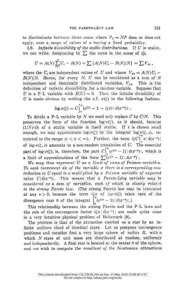
2.8. Infinite divisibility of the stable distributions. If U is stable, we can write, designating by E the sums in the sense of D3,

U = A(N) U, - B(N) = 1 {A(N)Ut - B(N)IN} = V

where the Ug are independent values of U and where VN, = A(N) U, - B(N)/N. Hence, for every N, U can be considered as a sum of N

independent and identically distributed variables, V, This is the definition of infinite divisibility for a random variable. Suppose that

U is a P-L variable with E(U) 0. Then the infinite divisibility of U is made obvious by writing the c.f. g)(-) in the following fashion:

log (?) = C (ecx -- ix) ! d(x-0) I

To divide a P-L variable by N we need only replace C by C/N. This preserves the form of the function log q(s), as it should, becaulse (1/N)-th of a stable variable is itself stable. If s is chosen small enough, we may approximate logcp(C) by the integral log9($, e), re-

stricted to the range (a < x < co). Further, the term itC x d(x-3) I

of log p(?, c) amounts to a non-random translation of U. The essential

part of log 9(?), is, therefore, the part C (e0x - 1) Id(x-0) , which is

a limit of approximations of the form (eiX - 1) I A(x-) 1. We may thus represent U as a limit of sums of Poisson variables.

To each increment dx of the variable x there is a corresponding contribution to U equal to x multiplied by a Poisson variable of expected value C d(x-c) . This means that a Pareto-Levy variable may be

considered as a sum of variables, each of wvhich is closely relatQd to the strong Pareto law. (The strong Pareto law may be truncated at any e > 0, because the term i<r of log p(O) takes care of the

divergence near 0 of the integral 5(et;2 - 1) Id(x-y) .)

This relationship between the strong Pareto and the P-L laws and the role of the convergence factor iXx I d(x-of) I are made quite ciear in a very intuitive physical problem of Holtsmark [9].

The problem is that of the attraction exerted on a star by an infinite uniform cloud of identical stars. Let us postpone convergence problems and consider first a very large sphere of radius R, with:n which N stars of unit mass are distributed at random, uniformly and independently. A final star is located at the center 0 of the sphere, and we wish to compute the resultant of thle Newtonian attractiots



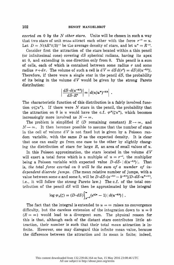
exerted on 0 by the N other stars. Units will be chosen in such a way

that two stars of unit mras6 attract each other with the force r-2 = u.

Let D = N(4R32r/3)-' be the average density of stars, and let u* = R-2. Consider first the attraction of the stars located within a thin pencil

(or infinitesimal cone) covering dS spherical radians, having its apex

at 0, and extending in one direction only from 0. This pencil is a sum of cells, each of which is contained between some radius r and some

radius r+dr. The volume of such a cell is d V = dSd(r3) = dS Jd(u-812)J.

Therefore, if there were a single star in the pencil dS, the probability of its being in the volume d V would be given by the strong Pareto

distribution:

| d Sd(u8) = d(u/u*) | dS.RB

The characteristic function of this distribution is a fairly involved func-

tion p(.u*). If there were N stars in the pencil, the probability that the attraction on 0 is u would have the c.f. qN(Cu*), which becomes

increasingly more involved as N - co.

The problem is simplified if (D remaining constant) R - co, and N -> co. It then becomes possible to assume that the number of stars in the cell of volume d V is not fixed but is given by a Poisson ran-

dom variable, with the same D as the expected density. It is clear that one can easily go from, one case to the other by slightly chang- ing the distribution of stars for large R, an area of small values of u.

In this Poisson approximation, the stars located in the volume d V

will exert a total force which is a multiple of u = r-2, the multiplier

being a Poisson variable with expected value D-dS. I d(u-312) 1. That is, the total force exerted on 0 will be the sum of a number of in-

dependent discrete jumps. (The mean relative number of jumps, with a

value between some a and some b, will be D.dS.(a-312 -b- '2)/D.dS.u*-'2, i.e., it will follow the strong Pareto law.) The c.f. of the total con-

tribution of the pencil dS will then be approximated by the integral

log p() = (D * dS) 2 (e';" - 1) I d(u-812)

The fact that the integral is extended to u = o raises no convergence

difficulty, but the careless extension of the integration down to u = 0 (R = o) would lead to a divergent sum. The physical reason for

this is that, although each of the distant stars contributes little attraction, their number is such that their total mean attraction is infinite. However, one may disregard this infinite mean value, because

the difference between the attraction and its mean is finite; indeed,



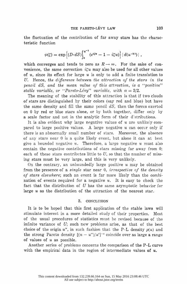
the fluctuation of the contribution of far away stars has the charac-

teristic function

R2

cp(I) = exp (D * dS) (eu" 1 -iu)} I d(zu3/2)

which converges and tends to zero as R - co. For the sake of con-

venience, the same correction itu may also be used for all other values

of u, since its effect for large u is only to add a finite translation to

U. Hence, the difference between the attraction of the stars in the

pencil dS, and the mean value of this attraction, is a "positive"

stable variable, or "Pareto-Le'vy" variable, with a 3/2. The meaning of the stability of this attraction is that if two clouds

of stars are distinguished by their colors (say red and blue) but have the same density and fill the samrre pencil dS, then the forces exerted on 0 by red or blue stars alone, or bv both together, differ only by a scale factor and not in the analytic form of their d stributions.

It is also evident why large negative values of u are unlikely com-

pared to large positive values. A large negative u can occur only if

there is an abnormally small number of stars. Moreover, the absence

of any stars nea-r 0 is a quite likely event, but alone it can at best

give a bounded negative u. Therefore, a large negative u must also contain the negative contributions of stars missing far away from 0;

each of these stars contributes little to U, so that the nuinber of miss-

ing stars must be very large, and this is very unlikely.

On the contrary, an unboundedly large positive u may be obtained from the presence oI a single star near 0, irrespective of the density

of stars elsewhere; such an event is far more likely than the combi-

nation of events required for a negative u. It is easy to check the fact that the distribution oi U has the same asymptotic behavior for large u as the distribution of the attraction of the nearest star.

3. CONCLUSION

It is to be hoped that this first application of the stable laws will stimulate interest in a more detailed stuidy of their properties. Most

of the usual procedures of statistics must be revised because of the

infinite variance of U; such new problenms arise, as that of the best choice of the origin u", in such fashion that the P-L density p(u) and

the strong Pareto density [(u - ut)/u']-t` coincide over as large a range of values of u as possible.

Another series of problems concerns the comparison of the P-L curve

with the empirical data in the region of intermediate values of u.



A final problem concerns the sign of a - 2. We have referred to

it several times, but a further discussion can be pursued only within the framework of a theory of P-L processes. (One indication may

already be found in Section 2 of [19J.) To settle this problem, it will probably be necessary to introduce some dependence between the addi-

tive components of U; this must be done carefully, however, if one

wants to avoid obtaining a wholly indeterminate answer. See also footnote 3.

International Business Machines Corporation, U. S. A.

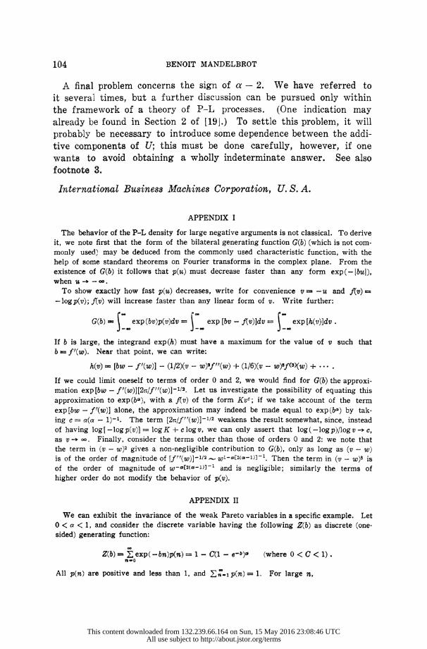
APPENDIX I

The behavior of the P-L density for large negative arguments is not classical. To derive

it, we note first that the form of the bilateral generating function G(b) (which is not com-

monly used) may be deduced from the commonly used characteristic function, with the

help of some standard theorems on Fourier transforms in the complex plane. From the

existence of G(b) it follows that p(u) must decrease faster than any form exp(-lbul), when u - .

To show exactly how fast p(u) decreases, write for convenience v -u and fv)

- log p(v); Alv) will increase faster than any linear form of v. Write further:

G(b) J exp(bv)p(v)dv = exp [by - fAv)]dv c exp [h(v)]dv.

If b is large, the integrand exp(h) must have a maximum for the value of v such that

b f'(w). Near that point, we can write:

h(v) [bw - f '(w)] - (1/2)(v - w)9f"(w) + (1/6Xv - w)88f()(w) + ' - '

If we could limit oneself to terms of order 0 and 2, we would find for G(b) the approxi-

mation exp [bw - f'(w)][2it/f"(w)]-112. Let us investigate the possibility of equating this approximation to exp(b'), with a flv) of the form Kvy; if we take account of the term

exp [bw - f'(w)] alone, the approximation may indeed be made equal to exp (bx) by taking c a(a - 1)-1. The term [21/f "(w)]-1"2 weakens the result somewhat, since, instead of having log [-log p(v)] a log K + c log v, we can only assert that log ( - log p)/log v -c as v - oo. Finally, consider the terms other than those of orders 0 and 2: we note that

the term in (v - w)2 gives a non-negligible contribution to G(b), only as long as (v - w)

is of the order of magnitude of [ff"(W)]-1/2 ~- W-1[2(*-1)]-1. Then the term in (v - W)3 is of the order of magnitude of W-([2(W.1)-l and is negligible; similarly the terms of higher order do not modify the behavior of p(v).

APPENDIX II

We can exhibit the invariance of the weak Pareto variables in a specific example. Let O < a < 1, and consider the discrete variable having the following Z(b) as discrete (one- sided) generating function:

Z(b) = - exp( -bn)p(n) = 1 - C(1 - e-b)0 (where 0 < C < 1) . n-0

All p(n) are positive and less than 1, and n I p(n) = 1. For large tn,



p()-Cn-(a,+') PC) r(- a)

The sum of two variables of this type has the generating function:

ZA(b) Z2(b) - 1 - 2C(1 - eb)* + C2(1 - e-1)2j

so that

P2(n) - 2Cn(+) - C2n-(2%+l) = 2p(n) + correction. [r(-a) r(- 2a)

For large n, the second part of the right-hand term becomes negligible compared to the

first. If a = 1/2, it is zero, so that the range of values of n in which it may be neglected

increases as a tends to 1/2. If 1 < a < 2, we must add a factor in (1 - e-b) to obtain an acceptable generating func-

tion; consider for example:

Z(b) = 1 - C(1 - e-b) + C'(1 - eb)

where 0 < aC' ? C ? C' + 1, so that C' ? (a - 1)-1. Now

2Cn-(04+1) 2CC'(a + 1)n-(,x1) C'2n-(2x+l)

r(- a) r(- a) '( - 2a)

For large n, the second and third terms become negligible for all a. The ratio of the

coefficients of the first and of the second term depends little upon a; but the ratio of

the coefficients of the third and first terms is ruled by r(- - a)Ir(- -2 a), which is zero for a 3/2, but may become large elsewhere. As a result, the range of values of n over

which the third term is important may be large.

Each time a increases past an integral value, the sign of C(1 - e-b) must be changed,

and another polynomial term must be added to Z(b), to keep it a generating function.

The number of corrective terms of p2(n) - 2p(n) increases, as well as the range of values of n in which the corrective terms are appreciable.

Similarly, as more than two terms are added, pN(n) - Np(n) is vitiated over an in-

creasing range of values of n. Let N -e oo, and observe the weighted sums of the varia-

bles Us, whose values are the integers n. (Z remains a summation in the sense of (B.) For 0 < a < 1, it is sufficient to consider the expression WN =N-" , since its

g.f. is ZN(N-1/ab), which tends to exp(-Cbm) when N --* co, as it should.

If 1 < a < 2, one must consider the expression WN = N-Il z ( Ut - M), where M, the mean value of Ut, is easily found to be C. The g.f. of WN is clearly exp(NCb)ZN(N-l Ib) and when N -*0o, it tends to exp (Cbm), as it should. It is easily seen that if we choose

for M a value different from C, the g.f. of WN will not tend to a non-degenerate expression.

If the value of a is higher, no linear renorming of Us can eliminate from log[Z(b)]

the square term Kb2, and hence, the best normed sum of the Us is the classically normed

N-112Z(Ui - M), which tends to a Gaussian, whatever the value of a.

APPENDIX III

This appendix concerns the transformation V=log U, which is used in most classical theories of income distribution.

The strong objections against this transformation do not apply at all in the case of a law due to Estoup and Zipf, which is formally similar to that of Pareto, but relates to word



frequencies, and which we have studied since 1951 (cf. [14], [16]). In the formal expression of that law U is replaced by the- "rank" of a word, where words are crdered by decreasing

frequencies. Hence log U has an intrinsic meaning as "cost of coding"; in particular,

the addition of "costs" is quite meaningful.

In the case of income, the transformation V=log U is justified in our [18] and [191, and in a more detailed article which ought to appear soon.

REFERENCES

[ 1 ] AITCHISON, J. AND J. A. C. BROWN, The Lognormal Distribution, Cambridge: Cam-

bridge University Press, 1957.

[ 2 1 CHAMPERNOWNE, G., Economic Journal, Vol. -63 (1953), pp 318 ff. [ 3 ] CHANDRASEKHAR, S., Reviews of Modern Physics, Vol. 15 (1943), pp 1 ff, (reprinted

in N. Wax, Noise and Stochastic Processes, New York: Dover, 1954).

[4] DARLING, D., Transactions of the American MUathematical Society, Vol. 73 (1952),

pP 95 ff. 15 1 EINSTEIN, A., The Theory of Brownian Motion, New York: Dover, 1956 (reprint).

[6] FRICHET, M., Comptes Rendus de l'Acadenie des Sciences, Paris, Vol. 249 (1959), p. 1837.

[7 1 GIBRAT, R., Les inigalitUs economiques, Paris: Sirey, 1932. [ 81 GNEDENKO, B. V. AND A. N. KOLMOGOROFF, Limit Distributions for Sums of In-

dependent Random Variables (English translation by K. L. Chung), Reading (Mass.):

Addison Wesley Press, 1954.

[91 HOLTSMARK, J., Annalen der Physik, Vol. 58 (1919), pp 577 ff. [10] IwVY, PAUL, Calcul des ProbabilitUs, Paris: Gauthier-Villars, 1925. [11] ----, Theorie de laddition des variables aUatoires, Paris: Gauthier-Villars, 1937

(second edition: 1954).

[12] , Processus stochastiques et mouvement Brownien, Paris: Gauthier-Villars, 1948.

[13] LYDALL, H. F., Econometrica, Vol. 27 (1959), pp 110 if.

[141 MANDELBROT, B., in Communication Theory, ed. Willis Jackson, London: Butter. worth, 1953.

[151 , Memoranduim of the University of Geneva Mathematical Institute, January 16, 1956.

[16] , in Logique, Langage et Thiorie de l'Information, Apostel, L., B. Mandel- brot and R. Morf, Paris: Presses Universitaires de France, 1957.

[17] , Memorandum of the University of Lille Mathematical Institute, Novem-

ber, 1957.

[181 - , Comptes Ren-dus de 1'Acad(mie des Sciences, Paris, Vol. 249 (1959), pp. 613-615.

[19] -, Comptes Rendus de l'Acadimie des Sciences, Paris, Vol. 249 (1959), pp. 2153-2155.

[20] , Comptes Rendus de l'Acadgmie des Sciences, Paris, Vol. 250 (1960), pp. 451-453.

[211 MANDELBROT, B. AND F. ZARNFALLER, to be published.

[22] MILLER, H. P., The Income of the American People, New York: J. Wiley, 1955. [23] HANNA, F. A., J. A. PECKHAM, AND S. M. LERNER, Analysis of Wisconsin Income,

(Vol. 9, Studies in Income and Wealth) New York: National Bureau of Economic

Research, 1948.

[241 PARETO, V., Cours d'Economie Politique, Lausanne and Paris: 1897. [25] WOLD, H. A. 0. and P. WHITTLE, Econometrica, Vol. 25 (1957), pp. 591 ff.


Documents

The Pareto-Lévy Law and the Distribution of Income · international economic reviewv may, 1 review ~~~~~vol. 1, no. 2 the pareto-levy law and the distribution of income* by benoit