Embed Size (px)
Citation preview
The paradox of
subjective well-being and tertiary education
An investigation of Australian data using a heterogeneity and
life-domain approach
By
Ioana Ramia
Thesis submitted in fulfilment of the conditions for the degree of
Doctor of Philosophy
School of Social Science and International Studies
University of New South Wales
2012

THE UNIVERSITY OF NEW SOUTH WALES Thesis/Dissertation Sheet
Surname or Family name: Ramia First name: Ioana Abbreviation for degree as given in the University calendar: PhD School: Social Science and Policy Faculty: Arts and Social Sciences Title: The paradox of subjective well-being and tertiary education. An investigation of Australian data using a heterogeneity and life-domain approach
Abstract 350 words maximum: (PLEASE TYPE)
In the well-being literature an association is commonly drawn between higher education levels and higher income, better health, better employment opportunities, or even happier marriages. Despite such objective outcomes, most socio-economic studies of well-being have identified a negative or zero relationship between subjective well-being (SWB) and higher educational achievement. However, there is little understanding of the grounds of this relationship. Some scholars, in explaining the link, have called for further research into the theoretical and empirical relation between education and well-being. Using empirical data from national surveys, this thesis explores the relation between SWB and higher educational achievement in the Australian context.
In this thesis, the relationship between SWB and higher educational achievement is conceptualised in a life-domain approach and by exploring the heterogeneity of SWB by higher education. The thesis employs cross-disciplinary theories, building on concepts from life course theory, stress research, quality of life theories, social capital theory and the capabilities approach to education. Time-series cross-sectional (TSCS) data from the Household, Income and Labour Dynamics (HILDA) in Australia survey, the Longitudinal Survey of Australian Youth (LSA) and the Australian Survey of Social Attitudes (AuSSA) was analysed.
The results challenge the well-being literature at both the methodological and theoretical levels. One of the key findings of the thesis is that accounting for differences in individuals’ conceptualisation of SWB is fundamental in the accurate evaluation of self-assessed well-being. The analysis establishes that the tertiary-educated (TE) and the non-tertiary-educated (NTE) have different concepts of ‘what counts’ towards their well-being. The negative relationship between tertiary educational achievement and SWB previously identified in the literature is found to be the result of biases or measurement errors incorporated in traditional, single-item measures of subjective well-being (such as overall satisfaction, or overall happiness). When an alternative, multiple-item measure of SWB is computed as the average of the levels of satisfaction with key domains of life, the tertiary-educated are identifiably more satisfied than the non-tertiary-educated. These findings allow for the conclusion that there is no ‘puzzle’ or ‘paradox’ of SWB and tertiary education in Australia.
Declaration relating to disposition of project thesis/dissertation
I hereby grant to the University of New South Wales or its agents the right to archive and to make available my thesis or dissertation in whole or in part in the University libraries in all forms of media, now or here after known, subject to the provisions of the Copyright Act 1968. I retain all property rights, such as patent rights. I also retain the right to use in future works (such as articles or books) all or part of this thesis or dissertation.
I also authorise University Microfilms to use the 350 word abstract of my thesis in Dissertation Abstracts International (this is applicable to doctoral theses only).
……………………...............… Signature
……………..………...………
Witness
……………...……....…
Date
The University recognises that there may be exceptional circumstances requiring restrictions on copying or conditions on use. Requests for restriction for a period of up to 2 years must be made in writing. Requests for a longer period of restriction may be considered in exceptional circumstances and require the approval of the Dean of Graduate Research. FOR OFFICE USE ONLY Date of completion of requirements for Award:
THIS SHEET IS TO BE GLUED TO THE INSIDE FRONT COVER OF THE THESIS

COPYRIGHT STATEMENT ‘I hereby grant the University of New South Wales or its agents the right to archive and to make available my thesis or dissertation in whole or part in the University libraries in all forms of media, now or here after known, subject to the provisions of the Copyright Act 1968. I retain all proprietary rights, such as patent rights. I also retain the right to use in future works (such as articles or books) all or part of this thesis or dissertation. I also authorise University Microfilms to use the 350 word abstract of my thesis in Dissertation Abstract International (this is applicable to doctoral theses only). I have either used no substantial portions of copyright material in my thesis or I have obtained permission to use copyright material; where permission has not been granted I have applied/will apply for a partial restriction of the digital copy of my thesis or dissertation.' Signed ……………………………………………...........................
Date ……………………………………………........................... AUTHENTICITY STATEMENT ‘I certify that the Library deposit digital copy is a direct equivalent of the final officially approved version of my thesis. No emendation of content has occurred and if there are any minor variations in formatting, they are the result of the conversion to digital format.’ Signed ……………………………………………...........................
Date ……………………………………………...........................

Originality Statement
‘I hereby declare that this submission is my own work and to the best of my
knowledge it contains no materials previously published or written by another
person, or substantial proportions of material which have been accepted for the
award of any other degree or diploma at UNSW or any other educational institution,
except where due acknowledgement is made in the thesis. Any contribution made to
the research by others, with whom I have worked at UNSW or elsewhere, is
explicitly acknowledged in the thesis. I also declare that the intellectual content of
this thesis is the product of my own work, except to the extent that assistance from
others in the project's design and conception or in style, presentation and linguistic
expression is acknowledged.’
Signed ……………………………………………..............
Date ……………………………………………..............

Acknowledgements
This thesis addresses not just a research question but also a personal curiosity. Almost
four years ago I enrolled in a doctoral program thinking that obtaining a PhD was the
next natural step in one’s education and career. Not before long, I started doubting this
initial thinking and wondered if investing time and energy in ‘yet another degree’ was
worthy. As I got closer to completion I became convinced that ‘spending that many
more years in school’, as my parents called it, was the right choice. Of course, now my
parents are proud of me, and I am proud of them. I want to thank them for having
allowed me to choose my paths in life, even if it meant being several continents away
for over a decade now, and for the continuous support and love they have provided me
with.
The past twelve months have been eventful and intense. With the support of my
supervisors Professor Elizabeth Fernandez and Professor Peter Whiteford I have
managed to see this project towards an end. I want to thank them for having provided
me with valuable feedback and guidance when the ‘natural’ feeling of ‘being stuck’
was about. I have also managed to feel good and proud about having experienced the
excitement of a PhD.
This, however, came at a cost. I would like to acknowledge my friends and their
understanding of my absence from the ‘social stage’.
I would like to make a last but not least important acknowledgement of ‘the best thing’
in my life. I didn’t think I would change my title from ‘Miss’ to ‘Mrs’ before having
experienced the ‘Dr’ first, but I did. My life has taken an unexpected but fortunate turn
when I have met and married the love of my life, Gaby. I have never dreamt I would
have someone like you in my life, but here you are. Your special way of being, your
attention to detail, the moral and emotional support you give me, and most importantly
the love you show me make every day an adventure.

Abstract
In the well-being literature an association is commonly drawn between higher
education levels and higher income, better health, better employment opportunities, or
even happier marriages. Despite such objective outcomes, most socio-economic studies
of well-being have identified a negative or zero relationship between subjective well-
being (SWB) and higher educational achievement. However, there is little
understanding of the grounds of this relationship. Some scholars, in explaining the link,
have called for further research into the theoretical and empirical relation between
education and well-being. Using empirical data from national surveys, this thesis
explores the relation between SWB and higher educational achievement in the
Australian context.
In the past decade subjective well-being has become an important item on the agenda
of governments and measures of subjective well-being are often used to assess the
costs and benefits of policies. Most governments and international organisations (such
as the OECD) regard SWB as the most comprehensive measure of wealth, replacing
traditional measures like Gross Domestic Product and some social indicators.However,
subjective wellbeing is a complex concept developed mainly through inferential
measures, individuals being asked to evaluate their wellbeing by answering either of
the two questions (or their close derivates): ’Generally speaking, how happy are you
these days?’ or “All things considered, how satisfied are you with your life?’.
Furthermore, psychologists argue that individuals have different perceptions of what
contributes to their well-being.
In this thesis, the relationship between SWB and higher educational achievement is
conceptualised in a life-domain approach and by exploring the heterogeneity of SWB
by higher education. The thesis employs cross-disciplinary theories, building on
concepts from life course theory, stress research, quality of life theories, social capital
theory and the capabilities approach to education. Time-series cross-sectional (TSCS)
data from the Household, Income and Labour Dynamics (HILDA) in Australia survey,
the Longitudinal Survey of Australian Youth (LSA) and the Australian Survey of
Social Attitudes (AuSSA) was analysed.
The results challenge the well-being literature at both the methodological and
theoretical levels. One of the key findings of the thesis is that accounting for

differences in individuals’ conceptualisation of SWB is fundamental in the accurate
evaluation of self-assessed well-being. The analysis establishes that the tertiary-
educated (TE) and the non-tertiary-educated (NTE) have different concepts of ‘what
counts’ towards their well-being. The negative relationship between tertiary
educational achievement and SWB previously identified in the literature is found to be
the result of biases or measurement errors incorporated in traditional, single-item
measures of subjective well-being (such as overall satisfaction, or overall happiness).
When an alternative, multiple-item measure of SWB is computed as the average of the
levels of satisfaction with key domains of life, the tertiary-educated are identifiably
more satisfied than the non-tertiary-educated. These findings allow for the conclusion
that there is no ‘puzzle’ or ‘paradox’ of SWB and tertiary education in Australia.
Generalising these results, the thesis argues that there should not be a ‘one size fit all’
measure of SWB. Instead, in order to identify sources of well-being, or to find ways to
increase well-being, researchers and policy makers should first understand what counts
for the SWB of target groups of individuals (for example for low, middle, and high
income groups, or males and females), then find the best means to increase their well-
being accordingly.

Table of Contents
Chapter 1 Introduction ................................................................................................. 1 1.1 Background: Subjective well-being and tertiary education in Australia ................. 4
1.1.1 Subjective well-being in Australia .............................................................. 4
1.1.2 Tertiary education in Australia ................................................................... 6
1.2 The heterogeneity of SWB, the paradox of SWB and tertiary education, and the central thesis question ....................................................................................... 8
1.3 Thesis objective, hypotheses, and central argument .............................................. 10 1.4 Significance of the research ................................................................................... 12 1.5 Structure of the thesis............................................................................................. 13
Chapter 2 A review of theoretical frameworks ........................................................ 16
2.1 Introduction ............................................................................................................ 16 2.2 Relative theoretical orientations ............................................................................ 16
2.2.1 Theories of quality of life .......................................................................... 16
2.2.2 Life-Course Theory ................................................................................... 20
2.2.3 Life-span development, life course and stressors ..................................... 21
2.2.4 Human Capital Theory ............................................................................. 26
2.2.5 Capabilities Approach .............................................................................. 28
2.3 Theoretical approach of the thesis ......................................................................... 30 2.4 Conclusion ............................................................................................................. 31
Chapter 3 Well-Being and Education: A review of literature and methods ......... 33
3.1 Introduction ............................................................................................................ 33 3.2 Definitions and terminology .................................................................................. 33
3.2.1 Well-being and Quality of Life .................................................................. 33
3.2.2 The evolution of well-being and quality of life concepts .......................... 36
3.2.3 Working definition of SWB........................................................................ 38
3.3 Determinants of well-being .................................................................................... 38 3.3.1 Socio-economic and demographic factors and subjective well-being ...... 39
3.3.2 Educational achievement and socio-economic and demographic factors . 43
3.3.3 Educational achievement and well-being ................................................. 46
3.3.4 Subjective well-being over the life curse .................................................. 49
3.4 Approaches for the measure of subjective well-being ........................................... 50 3.4.1 Subjective well-being approach ................................................................ 51
3.4.2 Satisfaction with life .................................................................................. 53
3.4.3 Happiness .................................................................................................. 54
3.4.4 Top-down and bottom-up approaches to subjective well-being ............... 55
3.5 The need for research and contribution to knowledge ........................................... 57 3.6 Conclusion ............................................................................................................. 58
Chapter 4 The method of study ................................................................................. 59
4.1 Introduction ............................................................................................................ 59 4.2 Secondary quantitative data analysis ..................................................................... 60 4.3 Secondary data sets ................................................................................................ 62
4.3.1 Household, Income and Labour Dynamics in Australia (HILDA) Survey62
4.3.2 Longitudinal Survey of Australian Youth (LSAY) .................................. 66
4.3.3 Australian Survey of Social Attitudes (AuSSA) ....................................... 68
4.4 The design of the analysis ...................................................................................... 69 4.4.1 Life-domain approach and the heterogeneity of subjective well-being .... 70
4.4.2 Specifications of the analysis and its limitations ...................................... 72
4.5 Methodological biases in quality of life research .................................................. 74 4.6 Conclusion ............................................................................................................. 78
Chapter 5 Findings: Satisfaction with life and satisfaction with domains of life .. 79
5.1 Plan of the chapter ................................................................................................. 79 5.2 Introduction to the analysis .................................................................................... 79 5.3 Changes in satisfaction between 2001 and 2009 ................................................... 81
5.3.1 Changes in overall satisfaction with life ................................................... 81
5.3.2 Changes in satisfaction with areas of life ................................................. 83
a. Mean levels of satisfaction between 2001 and 2009 ................................................. 83
b. Distribution of satisfaction with life and satisfaction with domains of life, 2009 .... 94
5.4 The single-item and multiple-item measures of well-being ................................. 100 5.4.1 Overall satisfaction and average satisfaction, 2009............................... 100
5.4.2 Overall satisfaction and average satisfaction between 2001-2009 ........ 103
5.5 Conclusion ........................................................................................................... 105
Chapter 6 Findings: The heterogeneity of SWB by education ............................. 107
6.1 Introduction .......................................................................................................... 107 6.2 Correlations between domains of life and satisfaction with life, 2001 and 2009 108 6.3 Impact of satisfaction with domains of life on SWB, 2001 and 2009 ................. 110
6.3.1 Well-being in 2009 .................................................................................. 110
6.3.2 Well-being in 2001, and comparison with 2009 ..................................... 113
6.4 Conclusion ........................................................................................................... 116
Chapter 7 Findings: The impact of socio-economic and demographic factors
on well-being ............................................................................................ 118 7.1 Introduction .......................................................................................................... 118 7.2 The model and data description ........................................................................... 118 7.3 Findings, 2009 ..................................................................................................... 120
7.2.1 Gender..................................................................................................... 123
7.2.2 Marital Status.......................................................................................... 123
7.2.3 Employment status .................................................................................. 124
7.2.4 Aboriginal and Torres Strait Islander (ATSI) background..................... 125
7.2.5 Culturally and Linguistically Diverse (CALD) background ................... 126
7.2.6 Geographic location ............................................................................... 126
7.2.7 Health status ........................................................................................... 126
7.2.8 Financial advantage/disadvantage ......................................................... 127
7.2.9 Age .......................................................................................................... 130
7.4 Findings, 2001 ..................................................................................................... 131 7.5 Conclusion ........................................................................................................... 134
Chapter 8 The life-course approach to subjective well-being ............................... 136
8.1 Introduction .......................................................................................................... 136 8.2 Overall Satisfaction and Average Satisfaction in adult life ................................. 137
8.2.1 Overview of the measures ....................................................................... 137
8.2.2 Findings .................................................................................................. 140
8.3 The heterogeneity of SWB by age ....................................................................... 141 8.3.1 Correlation analysis................................................................................ 141
8.3.2 Regression analysis ................................................................................. 142
8.4 Conclusion ........................................................................................................... 145
Chapter 9 Capabilities approach to subjective well- being and education .......... 147
9.1 Introduction .......................................................................................................... 147 9.2 Education in the light of the capabilities approach .............................................. 148
9.2.1 School retention and university participation rates................................ 148
9.2.2 Likelihood of school retention and higher education enrolment ............ 152
9.2.3 Reasons for leaving school and not attending tertiary education .......... 156
9.3 SWB during emerging adulthood and in the context of higher education ........... 159 9.4 Conclusion ........................................................................................................... 164
Chapter 10 Discussion and conclusion ................................................................ 166
10.1 Thesis overview and key findings ....................................................................... 166 10.2 Contribution to knowledge and methodological, theoretical and policy
prescriptions ........................................................................................................ 168 10.2.1 Methodological connotations of the findings .......................................... 169
10.2.2 Theoretical implications ......................................................................... 172
10.2.3 Policy recommendations ......................................................................... 174
10.3 Limitations and further potential for research ..................................................... 176
References .................................................................................................................. 179
Appendix A. Survey questionnaires ........................................................................ 191
1. HILDA questions on satisfaction with aspects of life ............................................... 191 2. LSAY questions on happiness................................................................................... 192 3. AuSSA questionnaire ................................................................................................ 193
Appendix B Supplementary analysis to Chapters 5 and 7 .................................... 194 1. Satisfaction with life and satisfaction with domains of life, distribution of the
population. Results complementary to Section 5.1 ............................................. 195 2. The impact of socio-economic and demographic factor on satisfaction with
domains of life in 2001 and 2009. Analysis complementary to Chapter 7. ........ 196 3. The impact of socio-economic and demographic variables on overall satisfaction
with life throughout the life-course ..................................................................... 206
Appendix C. Technical appendix ............................................................................ 207 1. Instrumentation or participation bias ......................................................................... 208 2. Satisfaction with life and happiness or cognitive and affective measures of
wellbeing ............................................................................................................. 213

1
Chapter 1 Introduction
For decades economists, sociologists and policy makers have been interested in
understanding ‘what makes the good life’, principally by exploring possible sources of well-
being (McKain, 1939; Sewell, 1940; Cottam, 1941; Hagood, 1941; Mangus, 1942; Bauer,
1966; Easterlin, 1974, 2004; Diener, 1984; Zapf, 1984; Schuessler and Fisher, 1985; Headey,
1988; Diener, Diener and Diener, 1995; Veenhoven, 1996; Noll, 2000; Cummins, 2000;
Diener, Lucas and Scollon, 2006; Muffels and Headey, 2009). However, there have been
frequent disagreements over how to measure and define well-being, and the terms ‘quality of
life’, ‘happiness’, ‘satisfaction’ or ‘well-being’ have often been interchangeably used (e.g.
Veenhoven, 1999; Cummins, 2000; Easterlin, 2007; Michalos, 2007; Oswald and
Powdthavee, 2007). Nevertheless, there is a generally accepted distinction between objective
(measurable) well-being, assessed through economic and social indicators1, and subjective
(self-assessed) well-being, consisting of three main components: positive affect (pleasurable
feelings), negative affect (un-pleasurable, painful feelings) and life-satisfaction2 (Diener,
1999).
Using survey data, empirical researchers have explored determinants of subjective
well-being (SWB)3by including demographic and socio-economic factors like age, gender,
geographic location, socio-economic and cultural backgrounds, or educational achievement
in multivariate equations to investigate observable factors that affect well-being. The findings
of such empirical explorations do not always align with general expectations. For example,
Inglehart (1990) finds that happiness4 follows a U-shape trajectory over the life-course, with
the youngest and oldest being happiest. Women traditionally report higher levels of happiness
than men but recently there has been a decline in their relative levels of happiness (Stevenson
and Wolfers, 2009). Married people are happier than singles (Diener, 1984; Mastekaasa,
1994), and, dependent of sociodemographic factors, having children increases the happiness 1Economic indicators such as Gross Domestic Product (GDP) or social indicators like life expectancy at birth,
literacy and numeracy rate, or unemployment rate.
2 Psychologist Ed Diener coined the term Subjective Well Being (SWB) as the empirically measurable aspect of happiness, and suggested these three components of SWB. These aspects of SWB are later discussed in Chapter 3, section 3.4.
3 Throughout this thesis ‘subjective well-being’ and ‘SWB’ are used alternately.
4 In Section 3.2.1 the distinctions between happiness, satisfaction, positive affect, well-being and quality of life are discussed. In this context, happiness refers to self-reported well-being, i.e. subjective well-being.

2
of couples (Myrskyla and Margolis, 2012). Money ‘buys happiness’, but only in a limited
fashion (Blanchflower, 2001), and the richest are not any happier than average wage earners
(Cummins, 2000). Having a tertiary degree does not increase self-reported well-being, despite
its socio-economic advantages (Veenhoven, 1999; Hickson and Dockery, 2008; Dockery,
2010). However, results from such multivariate analyses of determinants of happiness are not
consistent across countries (Hartog and Oosterbeek, 1998; Peiro, 2006).
Most research in social science has focused on the impact of these and other socio-
economic and demographic variables on subjective well-being (e.g.: Easterlin, 1974; Diener,
Diener and Diener, 1995; Headey, Muffels and Wooden, 2004; Stevenson and Wolfers, 2008;
Easterlin, 2007), the change in subjective well-being over time (e.g.: Easterlin, 1974;
Veenhoven, 1993), and the differences in subjective well-being between countries (e.g.:
Peiro, 2006; Veenhoven, 2006). Some studies have sought to assess differences between the
levels of subjective well-being reported by individuals from different demographic groups,
such as men and women (Blau, 1998; Bjornoskov, Dreher and Fischer, 2007), or variations in
subjective well-being by age (Plagnol, 2010) or by income group (Clark, Etile, Postel-Vinay,
Senik and Van der Straeten, 2005). However, less attention has been given to the impact of
education on subjective well-being (Dockery, 2010:12), the difference in the levels of
subjective well-being or the differences in ‘what counts’ for the subjective well-being of
individuals with varying education levels.
After a review of the subjective well-being literature, Dockery (2010) counts only six
empirical studies that had as a main concern the relationship between education and
subjective well-being: Hartog and Oosterbeek (1998); Hickson and Dockery (2008);
Michalos (2007); Ross and Van Willigen (1997); Stevenson and Wolfers (2008); and Witter
et al. (1984) (Dockery, 2010:14). Given that the area of subjective well-being has been
researched for more than eight decades, this is a surprisingly small number5.
The paucity of research matters because education is positively correlated with
objective well-being at both social and individual levels (human capital theory, Becker
(1962)), but recent studies have found that tertiary educational attainment makes a zero or
negative contribution to subjective well-being (e.g.: Veenhoven, 1996; Hartog and
5 Although the term subjective well-being was only coined in the 1980s (Diener, 1984), the area has been
researched for decades. A comprehensive insight into the development of the subjective well-being research is offered in Chapter 3, Section 2 of this thesis.

3
Oosterbeek, 1998; Cummins, 2000; Dockery, 2003; Hickson and Dockery, 2008). Such
studies have attempted to explain the controversial findingthrough various theories of well-
being such as the ‘adaptation’ theory, or the ‘hedonic treadmill’ theory (later discussed in
Section 2.2.1). However the complexity of the relationship has only recently come to the
attention of empirical researchers, such as Gong, Cassells and Keegan6 (2011), who have
called the negative or zero relationship between subjective well-being and tertiary
educational achievement ‘the puzzle of subjective well-being and higher education’ and
explored it using Australian survey data7. Some scholars (Desjardins, 2008; Dockery, 2010),
in explaining the link, have called for further research into the theoretical and empirical
relation between education and well-being (Dockery, 2010: 12; Desjardins, 2008: 33).
Through an original conceptualisation of subjective well-being in the context of
higher educational achievement, this thesis reassesses the relationship between subjective
well-being and higher education in Australia, using national data from secondary sources.
While acknowledging the benefits of qualitative data collection and analysis, a quantitative
approach is employed to explore the paradox8 of subjective well-being and higher educational
achievement.9 The main results draw on the pooled cross-sectional analysis10 of 2001-2009
Household, Income and Labour Dynamics in Australia (HILDA) survey data and a cross-
sectional comparison of the 2009 and 2001 data from the same source. HILDA data was
available on request from the Melbourne Institute of Applied Economic and Social Research,
6 Researchers at the National Centre for Social and Economic Modelling (NATSEM) within the University of
Canberra have recently begun a research project looking into the puzzle of higher education and subjective well-being. While their research is innovative in relation to the analysis of happiness in the light of education and age in Australia, their conceptualisation and theoretical grounds differ from those explored in this thesis.
7 Although this study uses the same data as the present thesis, their approach differs from the one employed here. These differences are discussed in Chapter 4 when the methodological approach of the thesis is explained.
8The availability of cross-sectional and longitudinal data in ready-to-use format (SPSS and Stata) is one of the main advantages of using secondary data sources. The economy of time and money given the limitations of a PhD research project are other important reasons why quantitative secondary data analysis is preferred to qualitative interviews. These aspects are further discussed in Chapter 4.
9 In this thesis, the negative relationship between SWB and higher education is referred to as ‘the paradox of SWB and higher education’, in line with other such controversial relationships such as the Easterlin Paradox (Easterlin, 1974).
10 Baird et al. (2008) explain how participating in consecutive year surveys that inquire about subjective well-being has an effect on respondents’ levels of SWB (i.e. a participation bias). Pooled cross-sectional rather than longitudinal analysis is hence preferred for the exploration of SWB across years. The reasons behind using a refreshed sample (repeated and fresh respondents), and not repeated samples of the same individuals are discussed in Chapter 4.

4
at the University of Melbourne. SWB was measured in this survey as satisfaction with eight
key aspects of life, and as overall satisfaction with life.
An alternative measure of SWB was explored in this thesis using data from the
Australian Survey of Social Attitudes (AuSSA), where SWB was measured as happiness.
This data however is limited in comparison with that available from HILDA, and the results
from this analysis are only reported in Appendix C.
To capture the moment of transition from school to tertiary education and work, the
subjective well-being of young people is analysed using data from the Longitudinal Survey of
Australian Youth (LSAY). The data was accessed from the Australian Social Science Data
Archive (ASSDA) at the Australian National University. The analysis conducted in this thesis
using the LSAY data is longitudinal and investigates how completing tertiary qualifications
affects the lives of young people. SWB is measured as happiness with life, and happiness
with key aspects of life. It must be noted however that the aspects of life investigated in this
survey are different from those in the HILDA survey. The main reason is that young people
assess their well-being through different items from those included in HILDA (such as school
performance, or getting along with parents and friends)
The reasons behind using these surveys, as well as the advantages of adopting a
quantitative rather than qualitative analysis, are discussed in Chapter 4. Although the
methodology employs secondary data analysis through econometric models, the theoretical
approach and conceptualisation place this thesis in the social science of well-being and not in
the economics of welfare or well-being. The findings have methodological and theoretical
implications, and social policy recommendations.
1.1 Background: Subjective well-being and tertiary education in Australia
This section offers background information to the study of subjective well-being in Australia.
Aspects of tertiary education in Australia, such as policy and participation, are also presented.
The importance of education to subjective well-being is discussed.
1.1.1 Subjective well-being in Australia
The term subjective well-being (SWB) was coined by Diener (1984).His article titled
‘Subjective Well-Being’ was published in the Psychological Bulletin in 1984 and has been

5
cited over 1300 times. SWB is often referred to as happiness, and various indicators to
measure SWB have been developed across decades.
The recent OECD (2011) report compares the percentages of people reporting more
positive than negative emotions in one typical day across member countries (Fig.1.1).
Australia ranks well above the OECD average, being in the top 30 per cent.
Fig 1.1 Percentage of people reporting more positive than negative emotion in one
typical day, 2010
Source: OECD (2011)
The acknowledged measure of SWB in Australia is the Personal Wellbeing Index
(PWI). The index was developed in 2001 by Professor Cummins at Deakin University as an
updated version of the Comprehensive Quality of Life Scale. The PWI is comprised of
questions on satisfaction with eight domains of life: standard of living, health, achieving in
life, relationships, safety, community-connectedness, future security, and spirituality/religion
(Cummins, 2006).
PWI uses an 11-point end-defined response scale, and satisfaction levels are ranked
from 0 to 10, with 0 being completely dissatisfied and 10 completely satisfied. For ease of
understanding and comparison with other well-being measures, the total is transformed to a 0
to 100 scale. The index is published quarterly to monitor the well-being of Australians.
Although minor changes do occur each quarter, the PWI maintains a mean value of around 75
(out of 100).
The Australian Unity Wellbeing Index (AUWI), assesses through subjective measures
how Australian feel about their lives and life in Australia. Both personal and national aspects
6
of satisfaction are ranked, for example, satisfaction with personal relationships, or satisfaction
with government. Results are published on the Australian Unity website11. Similar to the
levels of SWB measured through the PWI, since 2007 the AUWI has had values between 74
and 76 on a scale from 0 to 100.
A problem that is constantly discussed in the literature is the choice of domains of life
when the ‘multiple-item’ measure12 of SWB is computed. For example, psychologists argue
that using the same life-domains for individuals across all ages and stages of life is far from
straight-forward. This is because it is necessary to control for variations in stressors and
conceptualisations of well-being across stages of the life-course13. In this thesis the multiple-
item life domain satisfaction is computed using the levels of satisfaction with eight domains
of life: employment opportunities, financial situation, amount of free time, health, home,
local community, neighbourhood and safety14.
Although the measurement of SWB continues as a cross-disciplinary debate, more
governments have embraced subjective well-being as an important indicator of wellbeing, to
complement if not replace traditional economic measures of wellbeing such as GDP, GNP, or
utility. Hence the accurate and precise measure of SWB is of extreme importance, as
subjective well-being is becoming an important measure in shaping national policy.
1.1.2 Tertiary education in Australia
Following the European model, between 1974 and 1988 tertiary education in Australia was
free to all qualified students. However, from 1989 onwards a system of partial contribution to
the full cost of education was introduced through the taxation system. That system, called the
Higher Education Contribution Scheme (HECS) was designed so that students would make
compulsory payments only after they were earning a minimum amount in the paid labour 11http://www.australianunitycorporate.com.au/Community/auwi/Pages/results.aspx.
12 The multiple-item measure of SWB refers to the assessment of SWB by inquiring about satisfaction with various domains of life. The single-item measure of well-being on the other hand, inquires about satisfaction with life overall. These measures are discussed throughout the thesis, see Section 3.4.4.
13 This issue is complex and is discussed in-depth at various points across the thesis. In Chapter 3 the topic is addressed in the body of a literature review that presents the psychological aspects of the assessment of wellbeing. The debate is also discussed in the context of the findings, in Chapters 6, 8, and 9.
14 Testing whether the computation of an aggregate well-being measure from the levels of satisfaction with these domains of life is appropriate is reported in Chapter 5. The high levels of correlation between satisfaction with domains of life and overall satisfaction confirm the relevance of these items to overall satisfaction and the good fit of the aggregate measure for assessing SWB.

7
market, in most cases after completing their studies. Students also had the option of paying
up front, at a discounted rate (Marginson, 1993). The next major change in the costs of
Australian higher education came in 1997 when HECS rates were partially liberalised.
Student payments were differentiated according to the expenses involved in providing the
course, and to market demand. Postgraduate coursework programs gradually charged full fees
however, and with increased internationalisation and the opening up of education to overseas
students, fee incomes to education providers have increased significantly (Marginson and
Considine, 2000).
Access to tertiary education is not free, and access and equity have long been central
items on the agenda of education policy in Australia (Bradley, Noonan, Nugent and Scales
2008). The Department of Families, Housing, Community Services and Indigenous Affairs
(FaHCSIA, 2009) reports that about 55 per cent of Australian young people aged 15 to 24
who are no longer enrolled in education have not progressed further than secondary school,
and of these only about half have completed Year 12. The same report finds that education
completion rates are highly dependent on demographics like gender, socio-economic status,
indigenous status, or geographic remoteness
At the international level, although Australian young people perform well in
education compared to young people in other developed countries (FaHCSIA 2009),
Australia is losing ground, falling from 7th (in 1996) to 9th (in 2009) within the OECD
countries with respect to the percentage of 25- to 34-year-olds to have completed tertiary
studies. However, in the past two decades tertiary education in Australia has shifted from an
elite system to a mass, highly internationalised system (Ramia, Marginson, Sawir and
Nyland, 2011). Growth since 2000 has been particularly high, the percentage of Australians
aged 15 to 64 years who have obtained tertiary qualifications to Bachelor level or above
increasing from 17 per cent in 2001 to 23 per cent in 2009 (ABS, 2010).
The Review of Australian Tertiary Education, 2008 (the Bradley Review)
recommends that in order to remain competitive at international standards, Australia must
increase the percentage of young people aged 24 to 35 who have completed tertiary education
to 40 percent by 2020. In 2010, only 34 per cent of Australians age 24 to 35 years had
achieved a tertiary qualification. While such recommendations are appropriate in the context
of a global knowledge economy, it is important to ensure that socio-economic and

8
demographic factors do not become roadblocks to education and the objective and/or
subjective outcomes it brings.
The next section introduces the argument of the thesis and how subjective well-being
is conceptualised and analysed in relation to tertiary educational achievement.
1.2 The heterogeneity of SWB, the paradox of SWB and tertiary education, and the
central thesis question
True, we have a divine desire for knowledge and wisdom, but with knowledge come also differences of points of view.
(Lin Yutang, 1937:55)
Studies like Shin and Johnston (1978), Diener (1984) and Rojas (2004, 2006) argue that
individuals rarely have the same perception of what ‘happiness’ is, and focus on different
aspects of their lives when answering the generic questions, ‘How satisfied are you with your
life overall?’ or ‘All things considered, how happy are you these days?’ These differences
between individuals in terms of their perceptions of well-being are discussed in the literature
as the ‘heterogeneity’ of SWB (Rojas, 2009). The studies that have so far accounted for
heterogeneity (or between-groups differences) in reported well-being are relatively scarce and
have so far been reduced to exploring differences in well-being by gender (Crosby, 1982;
Blau, 1998; Bjornoskov, Dreher and Fischer, 2007), age (Plagnol, 2010), or income (Clark et
al., 2005). In Section 4.4.1 the heterogeneity of SWB is further discussed within the
conceptualisation of the Life-domain approach.
The objective of this thesis is to explore the paradox of SWB and tertiary education in
Australia. Because individuals have different perceptions of what contributes to their well-
being (Lin, 1947; Clark et al., 2005; Rojas, 2006; OECD, 2011), the heterogeneity approach
to SWB is proposed, arguing that there should not be a single measure of SWB for all
individuals. Instead, in order to identify sources of well-being, or to find ways to increase
well-being, researchers and policy makers should first understand what counts as SWB for
target groups of individuals (for example, low, middle, and high income groups, or males and
females), and then find the best means to increase their well-being accordingly.

9
Using Mexican data, Rojas (2004) explored the heterogeneity of SWB by
demographic characteristics through a life-domain approach. The life-domain approach
implies an evaluation of overall subjective well-being as the result of happiness or
satisfaction with various domains of life (e.g. work, financial situation, home, etc.). He found
that the importance of domains of life to the SWB of Mexicans varied across demographic
groups by age, gender and education level, thus showing the heterogeneous nature of SWB in
Mexico. Other studies that have taken some account for the heterogeneity of SWB(such as
Clark et al., 2005) argue that individuals in the same demographic groups would have similar
levels of SWB15. However minimal attention has been paid to the conceptual differences in
‘what counts’ when satisfaction or happiness are ranked. These conceptual differences are
important because not all individuals give the same weight or importance to aspects of life
when assessing ‘overall satisfaction’ or how ‘happy’ they are, ‘all things considered’.
The heterogeneity approach to SWB tested by Rojas (2004) in Mexico and proposed
for the purpose of this thesis accounts for differences in individual perceptions of what
‘counts’ as well-being. As a particular application of the approach, the thesis explores the
heterogeneity of SWB in the light of higher educational achievement in Australia to answer
the central research question: Is there a paradox of subjective well-being and higher
education in Australia?
The heterogeneity of SWB by educational achievement is embraced in this thesis and
SWB is separately assessed for individuals with tertiary studies at Bachelor level or above,
and for those without tertiary studies. The thesis aims to untangle the paradox of tertiary
education and SWB and is hence focused on exploring the differences in SWB that occur
between tertiary- and non-tertiary-qualified individuals. Additional disaggregation of the non-
tertiary-educated population by highest degree or school level (i.e. Certificate I, II, III or IV,
Year 12, Year 11, Year 10 and below), and that of tertiary-educated individuals by the
distinction obtained (Bachelor, Diploma and Advanced Diploma, Masters, Doctorate) is also
possible. However, these differences in SWB are outside the scope of the thesis. The aim is to
understand if, and if yes, why, the tertiary-educated have lower levels of subjective well-
being than the non-tertiary-educated (i.e. explore the paradox of SWB and tertiary education).
15 This similarity refers to the actual numeric level, usually on a scale from 0 to 10. A hypothetical example
would be that women have a level of SWB around 8.5 while men rank their SWB around the level 8.3. This would allow the conclusion that SWB is (empirically) heterogeneous by gender.

10
SWB is heterogeneous for other demographics such as gender, age or socio-economic
background as well, but identifying these levels of heterogeneity is also outside the scope of
this thesis.
The theoretical approach of the thesis builds explanatory support for the argument that
perceptions of well-being change with higher educational achievement. The thesis uses a
number of approaches to measuring well-being. In the subjective well-being approach (i.e.
exploring individual well-being through subjective measures), the measures of well-being are
inferential and subjective in nature (Rojas, 2004). In the ‘multiple discrepancies
theory’(MDT, Michalos, 1985),‘reported net satisfaction is a function of perceived
discrepancies between what one has and wants, relevant others have, the best one has had in
the past, expected to have three years ago, expects to have after five years, deserves and
needs’ (Michalos, 1985:347). In the capability approach, education is mapped as a capability
enabling individuals, and changing attitudes and expectations (Sen, 1985; Saito,
2003).Drawing on these theories, the thesis argues that perceptions of well-being vary across
the population and that SWB is heterogeneous by higher educational achievement. The socio-
economic and demographic variables that impact on the SWB of the tertiary-educated and
non-tertiary-educated are then investigated to explore whether, and if so, why there is a
paradox of SWB and higher education in Australia.
1.3 Thesis objective, hypotheses, and central argument
The central objective of this thesis is to explore the relationship between tertiary educational
achievement and subjective well-being in Australia. Three hypotheses have been generated to
serve this objective. The first hypothesis is designed to compare the levels of subjective well-
being of the tertiary-educated and the non-tertiary-educated using first a single-item measure
(overall satisfaction) and then a multiple-item measure (average satisfaction) derived from
the levels of satisfaction with domains of life. This first hypothesis is:
1) The highly educated a) are more satisfied with most aspects of life and b) are more
satisfied with life overall.
Hypothesis 1-a builds on human capital theory (Becker, 1964) and argues that
education enhances individual growth, and hence individual satisfaction with areas of life

11
such as work, health or wealth. Based on the life-domain approach16 to subjective well-being,
hypothesis 1-b proposes that the higher levels of satisfaction with most domains of life that
are associated with educational achievement translate into higher subjective well-being
(overall satisfaction with life).
The single and multiple-item measures of subjective well-being lead to diverging
conclusions with respect to the paradox of subjective well-being and higher education,
pointing to the need for further investigation.
The second hypothesis explores whether perceptions of well-being change with
tertiary educational achievement:
2) a) SWB is heterogeneous by higher educational achievement17 and b) socio-economic
and demographic factors impact the SWB of the tertiary-educated and the non-
tertiary-educated to a different extent.
The literature identifies a strong age effect of subjective well-being (Frey and Stutzer,
2002;Heady and Waren, 2008; Blanchflower and Oswald, 2004). Cross-disciplinary studies
argue that change in the stressors18 and perceptions of well-being throughout the life-course
arethe main cause of the large variations in SWB across the stages of life (Plagnol, 2010), and
especially during late adulthood (65 years and older). Employing a life-course approach to
SWB and drawing on life-course theory, life-span development and stress research19, the final
hypothesis of the thesis proposes that subjective well-being is heterogeneous by age, and
furthermore, that differences between the levels of subjective well-being of the tertiary-
educated and the non-tertiary-educated are likely to change throughout the life-course. The
third and final hypothesis of the thesis is:
16 It has been flagged on p.10 that the life-domain approach implies an evaluation of overall subjective well-
being as resulting from happiness or satisfaction with various domains of life. This approach is also discussed in Chapter 3, Section 4.
17 I.e. the factors that ‘count’ for the subjective well-being of highly educated and non-highly educated are not same.
18 Stressors are defined as the factors that create situations when ‘pressure exceeds one’s perceived ability to cope’ (Lazarus and Folkman, 1984). There are various types of stressors: eventful stressors (such as getting married, having children, having disruptive conflicts); chronic stressors, mainly caused by changes in the ambience; and quotidian stressors occurring at the micro level (Pearlin and Skaff, 1996). Section 2.2.3 discusses these conceptsin depth.
19These theories are discussed in-depth in Section 2.2.3where the importance of accounting for stages of life in subjective well-being research is argued.

12
3) a) SWB is heterogeneous throughout the stages of the life course and b) Socio-
economic and demographic factors that impact SWB vary throughout the life-course.
The results of the analysis stemming from the testing of the hypotheses are detailed in
Chapters 5 to 9, the results chapters. In summarising these results, the central argument of the
thesis is that subjective well-being is heterogeneous by tertiary educational achievement and
stage of the life-course. The findings of the thesis indicate that biases resulting from the
conceptualisation of subjective well-being shed light on the paradox of tertiary education and
subjective well-being. Bias is defined in the thesis as occurring when a response to a test item
tends to be altered in such a way that it indicates something other than what it is intended to
measure Runquist (1950).
The timeliness and importance of the research are discussed in the next section and
the wider contribution to knowledge of the thesis is discussed in Section 1.5.
1.4 Significance of the research
Current education policies promote increased participation in tertiary education in Australia
(Bradley et al., 2008). Nevertheless, recent Australian empirical studies conclude that
completing education at tertiary levels, while increasing the material (or objective) well-being
of individuals and societies, does not add to individual happiness or satisfaction with life
(Hickson and Dockery 2008; Dockery, 2010).
The zero or negative relationship between higher education and subjective well-being
has been identified both in Australia and internationally (Veenhoven, 1999, Hartog and
Oosterbeek, 1998, Peiro, 2006, Hickson and Dockery, 2008). However, few studies have
aimed to explore the bases of this relationship. Through a non-conventional approach this
thesis answers the need for a theoretical and empirical exploration of the relationship between
tertiary education and subjective well-being, by arguing the heterogeneous nature of
subjective well-being by higher educational achievement and age.
While the statistical computations and econometric models are not new, the
methodological and theoretical conceptualisations of the thesis bring novelty to the study of
subjective well-being in the field of the social sciences. The thesis argues that a ‘one size fits
all’ measure of SWB is not appropriate to assess SWB at national level as individuals have
different perceptions of ‘what counts’ for their well-being. The correlates of subjective well-

13
being are separately assessed for the tertiary-educated and non-tertiary-educated individuals,
their levels of overall subjective well-being are evaluated, and factors that increase the
subjective well-being of each group are explored. Differences by age are also considered.The
innovation of the thesis is the argument that the paradox of subjective well-being and higher
educational achievement is the result of perceptions and conceptual biases in the assessment
of the single-item measure of subjective well-being.
1.5 Structure of the thesis
In pursuit of the central research question, the remainder of the thesis is divided into nine
chapters. Chapter 2 discusses the theories that the thesis builds on, namely theories of quality
of life and the life-course, human capital theory, and the capability approach. Theories of
quality of life help develop an approach to the study of subjective well-being and a
theoretical explanation of the changes in self-reported well-being in the wider context of
overall well-being. Life-course theory, triangulated with aspects of life-span development,
underlines the importance of age-cohort effects in the analysis of ‘what makes the good life’.
This offers the theoretical grounding for further investigation of well-being across the stages
of life. And finally, human capital theory and the capabilities approach conceptualise tertiary
education as a life-changing event, worth of further investigation in the context of well-being.
Chapter 3 is a critical review of the relevant literature. Section 3.2 discusses the
confusion that often occurs between the terms ‘quality of life’ and ‘well-being’, offering a
working definition of subjective well-being for this thesis. Section 3.3 is an in-depth review
of the subjective well-being literature, and for this purpose four bodies of literature have been
distinguished. Studies that explored the relationship between socio-economic and
demographic factors and well-being are first reviewed, followed by a compendium of studies
that explored the relationship between these socio-economic and demographic factors and
education. The third body of literature is a critical review of studies that explored the
relationship between educational achievement and well-being. Finally, studies that take a life-
domain approach to explain well-being are reviewed to understand how the relationship
between well-being in areas of life and overall well-being has been discussed in the literature.
Section 3.4 discusses conventional methods that have explored subjective well-being,
andSection 3.5 explains how this thesis contributes to the subjective well-being literature
through its theoretical approach, its methodology and its conceptualisation of subjective well-
being in the context of higher educational achievement.

14
Chapter 4 addresses the methodological approach of the thesis. The advantages of the
life-domain approach are discussed. Differences in measuring subjective wellbeingand how
they are controlled for in the thesis are then detailed. The datasets and their limitations are
also explained, and the operational research questions that led to the testing of the hypotheses
are framed in the context of the empirical analysis.
Chapter 5 is the first chapter of analysis and results. Subjective well-being by higher
educational achievement is explored in the context of the adult population (over 25 years)
through a pooled cross-sectional analysis of the Household, Income and Labour Dynamics in
Australia (HILDA). The chapter starts with an investigation of the change in levels of
satisfaction with domains of life between 2001 and 2009. How the levels of satisfaction with
employment opportunities, finances, free time, health, safety, home, neighbourhood, and
local community have changed in the past decade is then explored, and the statistical
significance of the differences between the tertiary-educated and non-tertiary-educated is
mapped. The second part of the chapter explores in a life-domain approach the changes in
subjective well-being and in well-being in life domains between 2001 and 2009. Two
measures of subjective well-being are assessed: overall satisfaction with life, obtained as the
answer to the general question, ‘All things considered, how satisfied are you with your life?’;
and average satisfaction, calculated as the arithmetic average of levels of satisfaction with the
eight domains of life included in the satisfaction with life module of HILDA. The purpose of
the chapter is to explore the relationship between SWB and tertiary education using different
measures of SWB—overall and at life-domain level.
Chapter 6 uses the heterogeneity of SWB to explore the paradox of subjective well-
being and tertiary education. The heterogeneity of subjective well-being by educational
achievement is tested and the extent to which satisfaction with aspects of life impact on the
subjective well-being of tertiary- and non-tertiary-educated Australians is examined. Whether
socio-economic and demographic factors equally affect the subjective well-being of tertiary-
educated and non-tertiary-educated is explored in Chapter 7.
Chapter 8takes a life-course perspective, assessing the heterogeneity of subjective
well-being by educational achievement throughout each stage of the life-course. The analysis
is conducted using adult population data from HILDA, 2009.
The Longitudinal Survey of Australian Youth (LSAY) provides youth-specific
information, and the subjective well-being of young people is separately analysed in Chapter

15
9 using this data. How the subjective well-being of young Australians changes as they transit
from school to further education is explored in order to understand whether differences in
well-being at national levels are due to intrinsic characteristics and prevail from a young age,
or whether young people with tertiary qualifications are happier than their counterparts, but
become less happy later in life (Headey et al, 2004; Hickson and Dockery, 2008; Dockery,
2010). Access to education is also discussed in the light of the capabilities approach.
Chapter 10 discusses the findings of the thesis in the current socio-economic and
political context of Australia, assessing the policy implications. The chapter presents the key
findings and outlines the contribution to knowledge brought by this thesis through its
methodological, theoretical and policy implications. The short-falls of the analysis are
identified and potential for expansion of the topic is discussed.
The questionnaires from the national surveys used in the analysis of this thesis are
presented in Appendix A, and additional empirical results of the analysis are kept in
Appendix B. Technical computations of the data have been performed to control for various
methodological and conceptual biases, and are discussed in Appendix C, the technical
appendix at the end of the thesis.

16
Chapter 2 A review of theoretical frameworks
2.1 Introduction
Education is traditionally positively correlated with aspects of objective well-being such as
employment opportunities, income, wealth or health (Becker, 1962; Easterlin, 1974;
Veenhoven, 1996; Peiro, 2006; Bradshaw, Hoelscher, and Richardson, 2006). Despite such
objective advantages, it has been argued that the relationship between higher educational
achievements and measures of subjective well-being such as happiness or satisfaction with
life is zero or negative in developed countries (Hartog and Oosterbeek, 1997; Hickson and
Dockery, 2008; Stevenson and Wolfers, 2008; Dockery, 2010). However, studies focusing on
educational achievements and quality of life exclusively,20 underline a lack of coherent
theories linking the two concepts, as well as the need for further empirical and theoretical
investigation of the links between them (this need was expressed by Dockery, 2010: 12 and
Desjardins, 2008:33).
The purpose of this chapter is to discuss theoretical orientations relevant to the thesis
and how they interact to frame the theoretical approach for the analysis. The chapter is
structured in four sections. Section 2.2introducesthe relevant theories and explains how they
interact with the thesis. The theoretical framework of the thesis is formulated in Section 2.3.
2.2 Relative theoretical orientations 2.2.1 Theories of quality of life
Several theories of quality of life have been developed in the past 30 years, such as the
‘adaptation level’ or ‘hedonic treadmill’ theory (Brickman and Campbell, 1971),‘personality
theory’ (Costa and McCrae, 1980), ‘multiple discrepancies’ theory (MDT, Michalos, 1985),
‘dynamic equilibrium’ theory (Headey and Wearing, 1992), ‘set point’ theory (Lykken and
Tellegen, 1996), and the ‘homeostatic’ theory (Cummins, 1995). These frameworks are
summarised in Table 2.1 and their relevant aspects are discussed below.
Set point theory argues that individual levels of happiness are determined by
characteristics which one was born with or which are developed early in life; hence
individual happiness is bound to remain unchanged at original (intrinsic) levels (Lykken and
Tellegen, 1996). However, other scholars have questioned the accuracy of this theory and
20 In a review of quality of life studies in the past four decades, Dockery (2010) identified only six studies
exclusively concerned with the impact of educational achievement on quality of life.

17
argued that, as well as intrinsic characteristics, life goals are strong determinants of perceived
happiness (Headey, 2006). Furthermore, recent studies have shown that it is not only one’s
own goals that can change one’s level of happiness, but also the goals of others, for example,
a partner’s goals (Headey, Muffels and Wagner, 2010). Although some studies support the set
point theory, such as Brickman and Coates (1978) who have found similar levels of
satisfaction for lottery winners and paraplegics, others have found that, to the extent that it
depends on need-gratification, happiness is not necessarily relative (Veenhoven, 1990).
Similar to the set point theory, hedonic treadmill theory argues that individuals tend to
return to initial levels of happiness, regardless of the events that might temporarily change
their happiness (Brickman and Campbell, 1971). Homeostatic theory compares this
phenomenon to the tendency of the human body to maintain a constant temperature
(homeostasis), and support for it has been found in Australian data (Cummins, 2000). Despite
various theories in favour of the idea of a relatively stable, hardly fluctuating level of
subjective well-being, many scholars disagree. Veenhoven (1990: 1) argues that ‘happiness-
is-relative’ theories usually mistake ‘overall happiness’ for ‘contentment’. While contentment
implies a comparison of ‘life-as-it-is’ with ‘how-life-should-be’, he argues that happiness
does not entirely depend on comparisons, but also on how one feels, which in turn depends
on the gratification of basic bio-psychological needs. Furthermore, these needs don’t adapt
and they therefore represent ‘the limits of human adaptability’ (Veenhoven, 1990:1). Diener,
Lucas and Scollon (2006) make five revisions to the hedonic treadmill theory while not
totally rejecting it: first, individuals’ set points are not hedonically neutral; second,
individuals have different set points; third, a single person may have several set points;
fourth, set points can change under some conditions; and finally, individuals have different
levels of adaptability to external events (Diener et al., 2006:1).Although set-point theory,
hedonic treadmill theory and homeostatic theory offer explanations of the limited changes in
happiness that some individuals record over time, more theoretical development is necessary
to explain why some individuals react to change more (or less) than others, and by what
means, if at all, their levels of happiness may be increased.

18
Table 2.1 Relevant theories of quality of life
Theory Theoretical statement Author(s)
Adaptation Level Theory Overtime individuals form expectations of the future, called frames of reference. Events that are more favourable than these expectations generate positive emotions, while those that are less favourable evoke negative emotions.
Helson, 1948, 1964
Hedonic Treadmill Theory
Individuals tend to return to initial levels of happiness, regardless the events that might temporarily change their happiness
Brickman and Campbell (1971, 1972)
Personality Theory Five factors (the “Big Five”) describe the human personality: openness, conscientiousness, extraversion, agreeableness, and neuroticism. These personality factors have strong relationships to wellbeing, e.g. extraversion leads to positive affect and neuroticism to negative affect. The temperament version of personality theory suggests that certain personality traits like neuroticism and extraversion are enduring cognitive dispositions that directly affect wellbeing while other personality traits have an instrumental role.
Costa and McCrae, 1980 Costa and McCrae, 1991
Multiple Discrepancies Theory
Reported net satisfaction is a function of perceived discrepancies between what one has and wants, and what others have, the best one has had in the past, expected to have 3 years ago, expects to have after 5 years, and deserves and needs.
Michalos, 1985
Dynamic Equilibrium Theory
Self-esteem must be high enough to ensure that individuals feel confident about engaging in suitable behaviours and low enough not to feel complacent. The mood and satisfaction of individuals may be governed by the psychological system that evolved to maintain self-esteem.
Headey and Wearing, 1986, 1987, 1988, 1989 Headey, 2008
Set Point Theory One’s level of happiness is close to impossible to change because it depends on characteristics one was born with or which are developed early in life
Lykken&Tellegen, 1996
Homeostatic Theory Similar to homeostasis in the regulation of body temperature, the homeostasis of subjective wellbeing argues that mood and satisfaction regulate stability of well-being. Regardless of the ups and downs, the overall well-being tends to return to initial levels.
Cummins, 1998; Darven, Cummins and Stokes (2007)

19
In 1985 sociologist and philosopher Alex C. Michalos developed the multiple
discrepancies theory (MDT) asserting that:
Happiness and satisfaction are functions of perceived gaps between what one has and wants, relevant to others have, the best one has had in the past, expected to have three years ago, expects to have after five years, deserves and needs.
(Michalos, 1985:347)
The MDT covers several aspects of other quality-of-life theories such as adaptability
and relativity, and differentiates between happiness and satisfaction, the former being
regarded as cognition and the latter as affect. The theory has six basic hypotheses:
1. Reported net satisfaction is a function of perceived discrepancies between what one has and wants, relevant to others have, the best one has had in the past, expected to have 3 years ago, expects to have after 5 years, deserves and needs. 2. All perceived discrepancies, except that between what one has and wants, are functions of objectively measurable discrepancies, which also have direct effects on satisfaction and actions.
3. The perceived discrepancy between what one has and wants is a mediating variable between all other perceived discrepancies and reported net satisfaction.
4. The pursuit and maintenance of net satisfaction motivates human action in direct proportion to the perceived expected levels of net satisfaction.
5. All discrepancies, satisfaction and actions are directly and indirectly affected by age, sex, education, ethnicity, income, self-esteem and social support.
6. Objectively measurable discrepancies are functions of human actions and conditioners.
(Michalos 1985:347-8)
The relationship between higher education and reported well-being is explored in this
thesis in the context of Australian national data and the MDT. A controversial finding of
studies of well-being is that individuals over the age of 50 have the highest levels of
happiness, satisfaction and positive affect (Frey and Stutzer, 2002; Blanchflower and Oswald,
2004). The quality of life theories mentioned above (Diener et al. 2006) explain such findings
through concepts of adaptation, or of comparison with peers or past events. Most of these
concepts, however, share common ground with the life-course theory which explains the

20
human development throughout the life course. For these reasons, the life-course theory, its
approaches and interaction with this thesis are discussed in the next subsection.
2.2.2 Life-Course Theory
The analysis of human life and origins has long been the concern of sociologists, and the
need for a ‘longitudinal approach to life history’ has been emphasised since the 1920s
(Thomas, 1920). Longitudinal studies of children in the 1920s and 1930s came as an answer
when the cohorts were followed into youth and adulthood. However as results appeared, the
issues that arose ‘could not be addressed satisfactorily by available theories’ (Elder 1998:1).
Hence the life course theory(LCT) emerged in the 1960s, from necessity.
A life course is defined as ‘a sequence of socially defined events and roles that the
individual enacts over time’ (Giele and Elder, 1998:22). Life course theory has four key
principles: historical time and place; the timing of lives; linked or interdependent lives; and
human agency (Elder, 1998: 4). All of these contribute to the conceptualisation of SWB in
this thesis.
The first principle of the LCT states that the life courses of individuals are embedded
in and shaped by the historical times and places they experience over their life-times. This
principle touches one of the aspects embedded in measures of SWB, that perceptions of well-
being are partly the result of the environment one lives in. Although it is difficult to control
for the effects of time and place, it is important to acknowledge that scholarly findings are
representative of a particular group of individuals, with specific characteristics of time and
space. Accordingly, the findings and conclusions of this thesis are representative for the
Australian population over the age of 25. Although the results may be applicable to other
nations, particular aspects of the data used such as the time of collection, or the cultural
characteristics of the Australian nation can mean that the findings are unlikely to be
representative at the global level.
The second principle, the timing of lives, emphasises that the developmental impact
of a succession of life transitions or events is dependent on when they occur in a person’s life.
Based on this principle, and in the light of the literature suggesting a strong age effect on
SWB, the relationship between higher education and SWB is explored while accounting for
the stage of life at which individuals find themselves.

21
The third principle argues that lives are lived interdependently, and the network of
shared relationships expresses social and historical influences. Measures of SWB are highly
dependent on perceptions of the environment (Plagnol, 2010) and this third principle helps
conceptualise and discuss the peculiar increase in SWB after the age of 50 that is presented in
the literature.
Finally, the fourth principle, human agency, underpins the theoretical and
methodological approach. It argues that individuals construct their own life course through
the choices and actions they take within the opportunities and constraints of history and social
circumstances. In the light of this principle, ‘attending tertiary education’ is theorised as an
action that contributes to the construction of individual lives and societies. The objective
outcomes of this action have been widely discussed and it has been concluded that education
is a fruitful investment in human capital (Becker, 1964), generating individual and societal
growth. The thesis however explores the individual subjective outcomes, and how higher
education can change the life-course of individuals.
Complementing the second principle of the life-course theory (the timing of lives), the
significance of age to development is further explored in this thesis, drawing on life-span
development research. Santrock (2007) explains the importance of accounting not only for
chronological age, but also for biological age, psychological age, and social age, for a
complete analysis of individuals from a life-span perspective. These aspects are discussed in
the next section.
2.2.3 Life-span development, life course and stressors
Life-span development and life course
The division of the life span into periods is a social construction, ‘an idea of the nature of
reality that is widely accepted by members of a society at a particular time, on the basis of
shared subjective perceptions or assumptions’ (Papalia-Olds-Feldman in Fernandez, 2010:9).
Eight periods within the life span are generally accepted in western societies: infancy and
toddlerhood (birth to age 3); early childhood (3 to 6 years); middle childhood (6 to 11 years);
adolescence (11 to 20 years); young adulthood (20 to 40 years); middle adulthood (40 to
65years); and late adulthood (65 years and older) (Fernandez, 2010:12-13).
The relationship between age and SWB is controversial and has been explored in
cross-sectional and longitudinal studies (e.g.: Diener, Suh, Lucas and Smith, 1999; Casas,

22
Figuer, Gonzalez, Malo, Alsinet, and Subarroca, 2007; Krueger, Kahneman, Schkade,
Schwarz and Stone, 2009; Cummins, 2010). Some studies have found a negative relationship
between ageing and SWB (Wilson, 1967); others have found a U-shape relationship (with the
youngest and oldest reporting the highest levels of happiness) that disappears when factors
such as income, marriage, or employment are controlled for in fixed effects models (Frijeter
and Beatton, 2011);and others have given the relationship a different consideration by
accounting for morale (Kutner, Fanshel and Togo, 1956) or contentment (Veehnoven, 1984).
Despite the ongoing debate, lapses in the conceptualisation of SWB have been identified as
possible biases, and the source of the age and SWB paradox by studies such as Ryff (1989) or
Plagnol (2010).
This thesis accounts for the heterogeneity of SWB (also discussed by studies like
Rojas, 2004, 2006 or Clark et al., 2005) primarily from the perspective of educational
achievement. However, because age is an influential factor in perceptions of well-being, the
latter part of the analysis brings an additional layer to this investigation by exploring the
differences in SWB between the highly educated and the non-highly educated in thelight of
the life-course approach. In Chapter 8 the differences in SWB between the tertiary-educated
and the non-tertiary-educated are explored at four stages of development: emerging
adulthood; early adulthood; middle adulthood; and late adulthood (Santrock, 2007:13).
Following recent changes in the economic and historical context of developed
countries, developmental psychologists have reconsidered the stages of the life course.
Individuals aged 18-25 years, having left the dependencies of adolescence but not quite yet
into full-adulthood, are now assessed as being at an emerging adulthood stage, a period of
exploration of possibilities in work, love and worldview (Arnett, 2000:469). Although not
yet considered a developmental stage per se by sociologists, emerging adulthood has drawn
the attention of developmental psychologists as one of the periods of transition that ‘can often
be turning points in people’s lives’ (Santrock, 2007, p.14). Education, and in particular
tertiary education, and the transition from education to work are the life-changing events
during emerging adulthood. Hence 18- to 25-year-olds become important to the analysis of
this thesis, and their SWB and access to tertiary education are explored in Chapter 9.
23
Stressors over the life-course
Life-course theory emphasises the necessity to analyse human life at different life stages due
to the constant changes in the nature and quality of stressors, the exposure to these stressors
along the life span, and the change in access to resources. Lazarus and Folkman (1984) argue
that stress occurs as the result of an imbalance between demands and resources, or when
‘pressure exceeds one’s perceived ability to cope’. Pearlin and Skaff (1996) identify three
types of factors which cause stress and affect the life-course: eventful stressors; chronic
stressors; and quotidian stressors.
Eventful stressors refer to life-events such as getting a job, getting married, getting
divorced, having children, changing jobs, or having disruptive conflicts. The occurrence of
eventful stressors follows an inverted U-shaped relationship relative to age, reducing as
people pass through mid-life (Ensel, 1991). However two types of eventful stressors are more
likely to occur at later stages of life: the death of peers and the onset of illness and/or physical
impairments (Pearlin and Skaff, 1996:240).
Chronic stressors are represented by ambient, role and quotidian strains, and are likely
to appear along the life course at varying intensities. Ambient strains refer to changes in the
environment – the community or the neighbourhood. These can give the elderly especially,
not only feelings of un-safety and deteriorating surroundings, but also feelings of self-decline
and regret for the ‘good old days’. Role strains such as institutional roles, families and their
interpersonal relationships may be a source of severe distress. They reach their highest levels
during early and middle adulthood when responsibilities are relatively high. Health and
financial problems are considered two additional chronic strains that may increase in
frequency with age (Pearlin and Skaff, 1996:241).
Finally, quotidian stressors are stressors arising from the context of one’s micro-
environment and refer to ‘the hardships that are experienced in satisfying the logistical
requirements of daily life’ (Pearlin and Skaff, 1996). These stressors are considered to be
mainly related to physical capacities and become more obvious at the onset of old age in
daily activities such as walking to shops, climbing stairs, etc. However, either these stressors
are nullified and overtaken by positive events in elders’ lives, or, they are not reflected in
reported well-being(for whatever reason).This latter possibility is argued by studies like
Blanchflower and Oswald (2007) and other studies which have found the U-shaped
relationship between happiness and age.

24
Pearlin and Skaff’s study of life stressors and life course development (Pearlin and
Skaff, 1996) analysed coping, social support and mastery as partial explanations for people’s
different reactions to life stressors. Both understanding the change in life-stressors and the
adaptation to them are valuable resources for this thesis. They help to explore not only the
age and SWB relationship, but also that the relationship of education to SWB. How these life
stressors and adaptations to them happen throughout the life span is described below.
Coping
Coping behaviour has been defined as the development and use of adaptive skills across the
life course (Kahana, 1992). Pearlin and McKean Skaff (1996) have argued, however, that
individuals tend to focus on managing the meaning of events, rather than trying to change
difficult situations in their lives. And most frequently, meaning is the product of ‘one’s
unique cognitive manipulations’. For example, graduating from high school could mean that
the child is ready to enter the labour force and help the family financially, while in other
families it could mean that the child is ready to go to college. Meaning, then, is ‘shaped in
part by the life-course context of problematic circumstances’ (Pearlin and McKean Skaff,
1996:243). Two types of coping strategies in the management of meaning are: 1) comparison
with others who are situated in similar positions – and sometimes have more aggravated
stressors; and 2) shifting priorities to fit the changing reality – such as shifting a life domain
down the list of priorities. Interestingly, these coping strategies are mirrored in the quality-of-
life research concepts of multiple-comparison and adaptation (Michalos, 1985) discussed in
Section 2.1.
Blonna (2007) discusses two types of coping: emotion-focused coping (changing the
way one views potential stressors); and problem-focused coping (finding different ways to
manage the potential stressor, rather than seeking an alternative to it). The concept of coping
behaviour may in fact clarify two dilemmas which researchers in social science have
identified and which are addressed in this study: the U-shaped relationship between reported
happiness and age; and the lower levels of happiness reported by tertiary-education
graduates. For example, older people can nullify the negative effects of decreased mobility
and worsening health by comparing themselves to peers who are worse off, or by shifting
their priorities to less physical activities and accepting their physical restrictions (as argued
by Brandtstadter and Baltes-Gotz, 1990 in Pearlinand McKean Skaff, 1996:243). Similarly,
individuals in emerging and early adulthood can tend to compare themselves to more

25
successful peers, and especially those with higher levels of education and higher
expectations, and also set themselves goals that keep them constantly in a ‘working towards
it’ or ‘almost there’ frame of mind while feeling a lack of accomplishment. With reference to
another discipline, the concept of coping was used similarly in sociology but under a different
name: adaptation. Adaptation refers to a person’s change in attitude and actions to suit the
changes in their life (Diener, 1984), and explains paradoxes such as similar levels of
happiness between lottery winners and average wage earners, or paraplegics and people who
can walk (Diener et al., 1999). It is also one of the concepts at the foundation of studies that
argue the heterogeneity of SWB (Rojas, 2004).As well, it grounds the setting for this thesis in
theorising higher education as a life-changing event with echoes throughout the life-course.
Lazarus and Folkman (1984) further identify six types of coping resources: health and
energy; positive beliefs; problem-solving skills; social skills; social support; and material
resources. Some of these coping strategies are discussed by life-course researchers: Peralin
and Skaff also identify social support and mastery as key factors in the reaction to life
stressors. Some of these coping strategies are briefly discussed below, while their relevance
to this thesis is underlined.
Social Support
Social contact and social networks play an important role in supporting individuals,
especially as they age, reducing feelings of loneliness, traditionally correlated with low levels
of happiness. On the other hand, having seen ‘the fleet shrink’,21 apart from sadness and
feeling of temporality, through comparison, or – as conceptualised in social science – through
the relative evaluation of well-being, individuals tend to see themselves as ‘blessed’ or better
off. This concept also supports the idea that reports of well-being amongst population aged
over 65 are likely to be amplified by age-specific experiences.
Mastery
Mastery is defined as a global sense of control and has been proven to contribute to well-
being (Cohen and Edwards 1989;Ryff, 1989 in Pearlin and Skaff, 1996). It has a dual role in
the stress process: on the one hand it regulates the impact of stressors, while at the same time
21The convoy metaphor comes from Kahn and Antonuccy (1980), as a way of describing the situation where the
older people see most of their peers die, which results in feelings of loneliness and low levels of happiness.

26
it may be increased or decreased by exposure to stressor conditions (Skaff and Pearlin,
1994:243). In the case of old people, ‘domains of life over which people have lost a measure
of control are moved out of a position of centrality and are replaced by those over which
control is still exercised, such as balancing a chequebook. From the perspective of the
observer, this kind of priority may seem to take up limited life space, but to the aging person
it stands as salient evidence of continuing mastery’ (Pearlin and Skaff, 1996:243).
This concept further supports the methodological approach of this thesis. It can be
argued that the differences in skills and abilities between the tertiary-educated and the non-
tertiary-educated are differences of mastery. Furthermore, triangulated with the effects of
ageing, it may be argued that the highly-educated and non-highly-educated have different
levels of need for adjustment in activities.
2.2.4 Human Capital Theory
Education can be pure consumption or pure investment, or it can serve both these purposes.
(Schultz, 1960:571)
Although the concept of human capital was coming into usage as early as the 18th century,
members of the Chicago School of economic thought (Schultz,1961; Becker, 1964 and
Mincer, 1974) are the pioneers of what is currently referred to as the human capital theory.
Stated simply, the theory argues that individuals gain knowledge and skills through
education and training that increase their employability, make them more productive at work,
and generate positive outcomes for both the individual and the employer. In short, education
can be considered an investment in human capital. The returns to education have been
assessed at both private and social levels. Mincer (1974) estimated the private returns to
education by equating the present value of two constant earning streams and differentiating
between the times when they start flowing: one earning stream starts at year 0 (no further
investment in education),the other starts at year s, after having invested s years in education.
As compensation for postponing earnings, an extra year of schooling increases annual
earnings by the discount rate22. In other words, earnings grow multiplicatively by the
discount rate (J. Hartog and H. Oosterbeek in J. Hartog and H.M. van den Brink, 2007:7-9).
22 The discount rate is the internal rate of return, salary after s years of education less salary after no years of
education relative to the investment costs.
27
These rates of return to education are estimated to be between 5 and 15 per cent, varying
between countries and by demographics such as gender or geographic location.
Alongside financial benefits, education has positive effects on civic participation
(Milligan, Morettin and Oreopoulos, 2004), lower crime rates (Lochner and Moretti, 2004),
and higher life expectancy (Lleras-Muney, 2005). After a review of the relevant literature,
Lindahl et al (2007) conclude that the social returns are the same or slightly higher than the
private returns to education (p.33). While such objective advantages are clear outcomes at
private and social levels, there is little agreement on the extent to which education
participates to individual subjective well-being, and especially in developed countries such as
Australia (Dockery, 2010).
The Government’s committee on the future of higher education in Australia in the
1960s (the Martin Report, 1964) stated: ‘The Committee believes that economic growth in
Australia is dependent on a high and advancing level of education’ (p.1), and that individual
benefits ‘are only a fraction of the benefits accruing to society’ (p.5). This stance is currently
maintained: the most recent report on higher education (The Bradley Report, 2008)
underlines the necessity to increase the proportion of 18- to 35-year-olds holding tertiary
qualifications to 40 per cent by 2020, roughly double the year 2000 figure. The reasoning
behind setting such targets is mainly the need for international competitiveness and for
keeping up with technological advances requiring highly-educated employees. Despite the
fact that the positive outcomes for society and the economic growth that follow from
investing in education are hardly ever in doubt, there is a growing and ongoing debate over
the negative impact of higher education on happiness or satisfaction with life at the individual
level (Hartog and Oosterbeek, 1997; Hickson and Dockery, 2008; Stevenson and Wolfers,
2008; Dockery, 2010).
Human capital theory argues that there are both social and individual outcomes from
education. Methodological and theoretical concepts derived from theories of quality of life
(discussed in Section 2.2.1)support this thesis in arguing that tertiary education does increase
the subjective well-being of Australians. Understanding that choices (such as obtaining
tertiary qualifications) are not always voluntary but possibly constrained by social, economic
or environmental conditions (principle 4 of life course theory), the capability approach (Sen,
1985) triangulated with aspects of the life-course theory provides further theoretical support
for the ways in which education helps individuals construct their own life course.

28
2.2.5 Capabilities Approach
Welfare economist and philosopher Amartya Sen developed the concept of capabilities and
the capabilities approach in the 1980s, arguing for the importance of freedoms in the
assessment of a person’s advantage, individual difference in the ability to transform resources
into valuable activities, and the multivariate nature of activities that give rise to happiness
(Sen, 1984; 1985). Sen distinguishes between the achievements of a person (what he or she
manages to do or be – functionings), and their capabilities (the person’s ability to achieve
certain functionings). He explains the concept of capability in a rather straight-forward
manner as the difference between choosing A when B is also available and choosing A when
B is not available, or what Sen describes as ‘real freedoms’ (Sen et al., 1987: 36-37). He
refuses to give a list that would constitute ‘objectively correct’ capabilities (Sen, 1984:47),
but makes a point about basic capabilities that are ‘intended to separate out the ability to
satisfy certain crucially important functionings up to certain minimally adequate levels’ (Sen,
1993:41).
Following Sen’s theoretical approach, political and feminist philosopher Martha
Nussbaum further developed the capability approach, which she considers ‘the most
important theoretical development in human rights during the past two decades’ (Nussbaum,
2007). Unlike Sen, Nussbaum creates a list of ten ‘central human capabilities’ that ought to
be on the agenda of every government of a developing country: life; bodily health; bodily
integrity; senses; imagination and thought; emotions; practical reason; affiliation; other
species; play; and political and material control over one’s environment (Nusbaum, 2000: 72-
5).
Both Sen and Nussbaum argue that the capabilities of human beings should not be
allowed to fall below a certain floor, which they see as their basic human rights. Nussbaum
argues that what individuals are capable of doing depends on combined capabilities, which in
turn depend upon internal and basic capabilities. However, the internal, as well as the
combined capabilities, depend on external conditions that are the domain of public and
political action.
Tertiary education can be theorised in terms of the capabilities approach in more than
one way. Firstly, having completed tertiary education is a proof of agency and draws
unquestionable outcomes, i.e. functionings. However, external factors, such as socio-
economic disadvantage, may impede the option of participation in tertiary education. Access

29
to education is present on any ‘list’ of capabilities: reading and communicating; taking part in
literary and scientific pursuits (Sen, 1984); or (the fourth capability on Nussbaum’s list of
ten) ‘senses, imagination and thought’ (Nussbaum, 2000). There is a distinction between the
basic right to education and the ability to complete higher education – a combined capability
dependent not only on basic and internal capabilities but as well on external conditions – and
this is analysed in this thesis in the context of higher education in Australia. Although nations
have the freedom to decide their own lists of capabilities in their internal Human
Development Report, the international report of the United Nations Development Programme
(UNDP, 2010) lists tertiary enrolment among the basic needs of literacy, as well as primary
and secondary education.
Within the capabilities approach, Sen and Nussbaum share two basic assumptions
regarding education: that humans are ends, not means, and that therefore the education of
humans should be concerned with realising freedoms and acknowledging diversity; and
secondly, that education is both instrumentally and intrinsically valuable for human
flourishing. They perceive that education is a basic capability promoting freedom and the
agency to participate further in education and to enlarge freedoms – a perspective which
contrasts with a commodified notion of education, that is, that only a basic minimum of
schooling is necessary. However, the social context can constrain or enlarge capabilities for
education and in education.
Using data from the Longitudinal Survey of Australian Youth (LSAY), the process
whereby university students and graduates are ‘selected’ is investigated in Chapter 9 of the
thesis. This chapter also investigates whether the choices to opt out of tertiary education are
voluntary or whether they are imposed on young people by the ‘constraints of history and
social circumstances’ (life course theory, Elder, 1974). The life course theory principle of
human agency, that individuals construct their own life course through the choices they make
and the actions they take within the opportunities and constraints of history and social
circumstances, takes the capabilities approach one step further to understand the impact of
capabilities, or alternatively of a lack of capabilities, on the life course.
30
2.3 Theoretical approach of the thesis
All of the theoretical frameworks reviewed above imply, directly or indirectly, that tertiary
education has a positive impact on well-being23.This thesis explores whether this is the case,
focusing, however, on the subjective aspect of well-being.
The springboard for the analysis contained in the thesis is the heterogeneous nature of
subjective well-being, in the notion that ‘what counts for happiness is everyone’s opinion’
(Lin, 1940 in Rojas, 2004). The thesis agrees with those authors who argue against a global
measure of subjective well-being, while holding that scholars and governments should aim to
understand what counts for groups of individuals, and explore ways of increasing the well-
being of targeted groups of individuals (e.g. low, medium and high income, male and female,
rural and urban). The central argument of the thesis is that what counts for the subjective
well-being of the tertiary-educated is different from what counts for the subjective well-being
of the non-tertiary-educated.
In explaining the negative relationship between subjective well-being and tertiary
education previously observed in the literature, the thesis follows multiple discrepancies
theory (MDT) in arguing that individuals tend to assess their well-being as functions of
perceived gaps between what one has and wants, with reference to what others have, and the
best one has had and expected to have in the past, expects to have in the near future, and
deserves and needs (Michalos, 1985). The thesis also includes the view that life stressors
change over time and with them the perceived well-being of individuals, as argued by stress
theorists such as Blonna (2007) and empirical researchers such as Pearlin and Skaff(1996).
Such studies have focused on the change in perceptions of well-being over the life-course.
However, change in the perceptions of well-being has not yet been explored in relation to
education. This thesis addresses this gap by exploring the heterogeneity of subjective well-
being by tertiary educational achievement.
Studies which have explored factors that affect subjective well-being in Australia
identify a negative or nil impact of tertiary education (e.g. Headey and Wooden, 2004;
Dockery, 2010). Nevertheless, human capital theory argues that education and training are
the most valuable investments in human capital, with positive outcomes at both the social and
23 Well-being understood, according to the OECD definition, as the material, environmental and subjective
aspects of well-being. The thesis, however, focuses on the subjective well-being aspect of overall well-being.

31
individual levels (Becker, 1964). Education is assessed in this thesis both as a capability
enabling further functionings (Sen, 1984) and, as argued by life-course theory, through the
principle of agency, that is, that individuals construct their own life course through the
choices and actions they take within the opportunities and constraints of history and social
circumstances (Elder, 1998). Finally, drawing on MDT, the thesis argues that discrepancies
between reality and perceptions, and the effects of various factors on an individual’s
assessment of their own achievements, result in misperceptions of subjective well-being;
hence the lower levels of subjective well-being reported by individuals with tertiary
qualifications.
The heterogeneity of subjective well-being by age is also explored. A life-course
approach to subjective well-being is undertaken, proposing that age-cohort-specific life
stressors (Ryff, 1989) that become the drivers of perceptions (Pearlin and Skaff, 1996)
translate into differences (or biases) in self-reported well-being along the life span.
The key principles of life course theory underline the importance of historical time
and place, the timing of lives, linked or interdependent lives, and human agency (Elder, 1998:
4). The first two principles argue the importance of age-cohort control, while the last two,
triangulated with the capabilities approach, underline the necessity to assess the impact of
life-changing events (such as attending higher education) throughout the life span.
By understanding tertiary education as a capability or investment in human capital
which enhances the functioning of both individuals and society, and by arguing the
importance of cohort biases in self-assessed well-being, the relationship between tertiary
education and subjective well-being in Australia is reassessed.
2.4 Conclusion
The purpose of this chapter has been to summarise relevant theoretical concepts and
formulate a theoretical framework for the hypotheses of the thesis to build on. How theories
of quality of life, life-course theory, life-span development and stressors, human capital
theory and the capabilities approach help conceptualise this thesis was discussed in Section
2.2. Section 2.3 formulated the theoretical framework of the thesis and stated its argument.
The next chapter is an in-depth review of relevant bodies of literature that complement
the theory reviewed in this chapter. Its objective is to assemble a background for the analysis

32
undertaken by the thesis. The gap in the literature is identified and how the thesis helps to fill
the gap through its theoretical and methodological innovations is explained.

33
Chapter 3 Well-Being and Education: A review of
literature and methods
3.1 Introduction
The aim of this chapter is to offer an up-to-date, in-depth review of studies that directly or
indirectly explore the relationship between educational achievement and subjective well-
being. The literature reviewed is critiqued in the light of the theoretical framework
formulated in Chapter 2, drawing mainly on quality-of-life theories (multiple discrepancies
theory), life-course theory, human capital theory and the capabilities approach.
The chapter is structured in six sections. Section 3.2 is a discussion of the distinctions
between the terms quality of life, well-being, and objective and subjective well-being,as these
have been discussed in the literature. The purpose of this section is to position the thesis
within the broader field of literature on the social science of quality of life, and to formulate a
working definition of subjective well-being. Section 3.3 is an in-depth review of the
subjective well-being literature. The studies reviewed in this section arestructured into four
main bodies of literature: first, studies that explore the relationship between education and
well-being; second, studies that explore the relationship between education and other socio-
demographic factors; third, studies that explore the relationship between well-being and
socio-demographic factors; and finally, studies investigating subjective well-being over the
life-course. Section 3.4 reviews methodological approaches to the study of subjective well-
being. Section 3.5 discusses the gaps in the literature and the contribution of this thesis to the
scholarly debate.
3.2 Definitions and terminology
3.2.1 Well-being and Quality of Life
The OECD (2011) recognises three dimensions of individual well-being: quality of life;
material living conditions; and sustainability of well-being over time. Income and wealth,
jobs and earnings, and housing are the material living conditions. The components of quality
of life identified by the OECD are health status, work and life balance, education and skills,
social connections, civic engagement and governance, environmental quality, personal
security, and subjective well-being. The sustainability of well-being over time refers to the

34
preservation of different types of capital: natural capital, economic capital, human capital,
and social capital (OECD, 2011:19, Fig. 3.1).
Fig. 3.1 Components of well-being
Source: adapted from OECD (2011: 19)
All these dimensions of individual well-being are essential to a comprehensive
exploration of general well-being. However, because the purpose of the thesis is to explore
the paradox of subjective well-being and tertiary education, only subjective well-being is
explored here, explained further in Section 3.4.1.
Quality of life and well-being have been addressed in a variety of fields such as
anthropology, economics, medicine, philosophy, politics, psychology, or sociology. While a
review of studies from all these fields would represent a thesis all in itself, for the purpose of
this chapter and the thesis as a whole, only the past four decades of socio-economic well-
being research is reviewed. Studies that address well-being in the fields of medicine and
psychology have proven especially fruitful to the conceptualisation of the thesis. The focus is
INDIVIDUAL WELL-BEING Quality of Life Material Living Conditions Health status Income and wealth Work and life balance Jobs and earnings Education and skills Housing Social connections Civic engagement and governance Environmental quality Personal security Subjective well-being
SUSTAINABILITY OF WELL-BEING OVER TIME (Requires preserving different types of capital)
Natural capital
Economic capital Human capital Social capital
35
on studies that investigate well-being from a bottom-up perspective24, seeking to understand
how well-being in particular areas of life, together with socio-economic and demographic
characteristics, affects overall well-being. An in-depth critical review of social science,
economic and relevant cross-disciplinary studies (as well as the medical and psychological
research) has been conducted, and the relevant findings are discussed in the remainder of this
section.
First, a tendency has been identified in social science either to use the terms quality of
life and well-being interchangeably, or to use one term to define the other (studies like
Headey and Wearing, 1992; Veenhoven, 1999; Cummins, 2000; Ferris, 2004). Some studies
(e.g. Farquhar, 1995) have pointed tothe lack of theoretical frameworks and the need to
conceptualise quality of life before conducting cohort-specific, life-domain-specific, or field-
specific quality-of-life analysis. It is also necessary to distinguish between individual-level
and population-level quality of life (Rapley, 2003). This thesis explores individual-level
subjective well-being.
Another major note in the literature is the necessity to assess quality of life from both
objective and subjective perspectives (Diener and Suh, 1997; Cummins, 1999; Noll, 2001;
Stutzer and Frey, 2010). Objective quality of life can be assessed through economic
indicators and objective social indicators such as health or safety (Erikson, 1993; Noll,
2001).However, due to its assessment at a personal level, subjective well-being is a complex,
non-forward measure of quality of life (Diener and Suh 1997; Haas1999; Noll 2002; Stutzer
and Frey 2010), and happiness and satisfaction with life are the traditional ways of assessing
it (Diener et al., 1999; Cummins, 2000; Headey and Wearing, 2010). Time-accounting
methods (Justin1985; Kahneman and Krueger 2006) which evaluate the flow of emotional
experience during daily activities, are alternative ways to measure quality of life. Subjective
well-being is assessed in this thesis using measures of satisfaction with life, assessing both
overall satisfaction with life and satisfaction with domains of life. These aspects follow the
recommendation in the literature, that researchers should be aware of the distinction between
overall and domain-specific well-being. These refer to satisfaction with areas of life such as
personal health, relationships, achieving in life, community-connectedness and future
24 The bottom-up approach argues that high levels of satisfaction with areas of life such as work, family or
health have the ability to increase overall well-being. It is contrasted with the top-down approach. Both approaches are further discussed inSection 3.4.4.
36
security(discussed by Diener 1999, Veenhoven 1999 and Cummins 2000, among others).
Various indices have been utilised across countries to account for life-domain-specific well-
being, and the Personal Wellbeing Index (PWI) is the most representative measure of
subjective well-being for Australia. The index investigates satisfaction with eight domains of
life: standard of living; health; achieving in life; relationships; safety; community-
connectedness; future security; and spirituality/religion (Cummins, 2006). However, there is
a question about whether some domains of life should be given greater weight in the
computation of the index, and if so, by which means should such weights be allocated. The
analysis in this thesis does not use the PWI to explore satisfaction with life and satisfaction
with domains of life, but data from the Household, Income and Labour Dynamics in Australia
(HILDA) survey.
Evaluating the overall and the domain-specific dimensions of quality of life raises a
further question about the direction of causality, whether satisfaction in various areas of life
generates an overall satisfaction, or whether a general high satisfaction with life generates
satisfaction in various domains (Diener et al., 1999). The causality from life-domain to
general satisfaction is investigated by those studies that take a bottom-up approach, while
those looking at the spill-over of general happiness on satisfaction with domains of life are
top-down approaches. This thesis employs a bottom-up, life-domain approach to subjective
well-being. Such methodological computations are further discussed in Chapter 4.
3.2.2 The evolution of well-being and quality of life concepts25
Although components of quality of life such as the ‘level of living’, employment status or
social status have been considered important in sociology since the 1920s (Ferriss, 2004), the
concept of quality of life was coined only much later on, in the 1960s, and the term was
finally indexed in the Sociological Abstracts only in 1979 (Schuessler and Fisher, 1985).
25 Definitions of quality of life and well-being:
Wellbeing: the state of feeling healthy and happy (Cambridge Dictionary); the state of being or doing well in life; happy, healthy, or prosperous condition; moral or physical welfare (of a person or community) (Oxford English Dictionary)
Quality of life: the level of enjoyment, comfort and health in someone’s life (Cambridge Dictionary); the standard of living, or degree of happiness, comfort, etc., enjoyed by an individual or group in any period or place; an instance of this (Oxford English Dictionary)

37
Throughout the past four decades the terms ‘quality of life’and‘well-being’ developed
and gained recognition. Some scholars consider the terms conceptually different (e.g. Smith,
1973; Langlois and Anderson, 2002), others have used one term to define the other (Ferriss,
2004), and many use them interchangeably (e.g.Veenhoven, 1999; Cummins, 2000; Easterlin,
2007; Michalos, 2007; Oswald and Powdthavee, 2007).
Conceptions and definitions of well-being and quality of life have changed across the
decades. Initially the terms ‘quality of life’ and ‘well-being’ were conceptually different.
Smith (1973) theorised well-being as a concept measuring the objective life conditions of the
population in general, and quality of life as a subjective assessment of individuals’ lives.
Nearly four decades later, Gasper (2010) also argued that the two terms were conceptually
different, but in the opposite way to Smith (1973), that is, he considered well-being applied
more at individual level, and quality of life when discussing communities, localities, or
societies. He acknowledged, though, the broad range of meanings that the terms have, and the
frequent overlaps that occur (Gasper, 2010).
Farquhar (1995) reviews studies of quality of life across several disciplines and
identifies the term ‘quality of life’ as often referring to specific aspects, such as health-related
quality of life. Similarly, studies like Noll (2001) and Rapley (2003) underline the necessity
to specify the exact items the concept investigates. From a theoretical perspective, Haas
(1999) discusses concepts like well-being, satisfaction with life, functional status, or health
status as borderline cases in quality of life research, representing aspects of quality of life
(Haas, 1999:735).
Still, most social studies use the term ‘quality of life’ in conjunction or
interchangeably with ‘well-being’ (Veenhoven, 1999; Cummins, 2000; Easterlin, 2007;
Michalos, 2007; Oswald, 2007).

38
3.2.3 Working definition of SWB
The thesis acknowledges the approach to quality of life initiated by the Australian Centre on
Quality of Life at Deakin University:
Quality of life is both objective and subjective. Each of these two axes comprises several domains which, together, define the total construct. Objective domains are measured through culturally relevant indices of objective well-being. Subjective domains are measured through questions of satisfaction.
(Australian Centre of Quality of Life, 2012)
The framework developed by the OECD (Fig. 3.1) is more detailed as it includes material
living conditions, quality of life aspects such as health status, work and life balance,
environment and subjective well-being, and the sustainability of well-being over time. In this
thesis, subjective well-being is identified as the subjective component of quality of life, being
classified as a component of the overall individual well-being.
3.3 Determinants of well-being
It is common in socio-economic studies to explore determinants of well-being by including in
multivariate analyses factors like age, gender, socio-economic status, geographic location,
income or health. Subsection 3.3.1 reviews such studies while focusing on the factors of
interest to this analysis: gender, income, health, marital status and employment status26. In
Subsection 3.3.2 studies that address the relationship between these socio-economic and
demographic factors and education are reviewed. The reason for the review of this body of
literature is to understand the possible spill-over effects from education onto subjective well-
being via outcomes like higher income or better health (as argued in studies like
Blanchflower and Oswald 1994 and Cummins 2000). Subsection 3.3.3 reviews studies that
directly or indirectly address the relationship between educational achievement and well-
being. Finally, the relationship between age and subjective well-being is discussed in
Subsection 3.3.4, laying the groundwork for the analysis of well-being by stage of the life-
course in Chapter 8.
26 The reasons for having selected these socio-economic and demographic factors are discussed in Chapter 4,
Section 4.4 when the datasets that are being analysed in this thesis are discussed.

39
3.3.1 Socio-economic and demographic factors and subjective well-being
An in-depth review of empirical studies in the fields of the sociology and economics of
happiness, complemented by results from medical and psychological research, has revealed
concave relationships between socio-demographic factors like income, age, social relations,
employment and education on the one hand, and subjective well-being on the other. For
example, work that involves a mental challenge brings satisfaction, but too much mental
challenge can reduce satisfaction to levels as low as that from jobs with no mental challenge
at all (Clark, 1996). Some studies find upper-secondary graduates to be happiest, although
higher education has a negative impact on happiness (Hickson and Dockery, 2008). Income
increases happiness only to a certain extent, then it ceases to have a positive impact
(Cummins, 2000; Easterlin, 2004). How these socio-economic and demographic factors relate
to subjective well-being is discussed below.
Income
The relationship between income and subjective well-being is particularly important to the
exploration of the relationship between education and subjective well-being due to the
indirect, positive effect that higher educational achievement has on employment opportunities
and salary rates (OECD, 2011). The relationship between income and happiness has been
debated since the beginning of scholarship on the economics of happiness. Easterlin (1974)
analysed the economic development and happiness of nations and noted that, although an
increase in personal income generated higher levels of happiness of individuals, countries
with high levels of economic growth did not report national levels of happiness higher than
developing nations. This phenomenon came to be known as the ‘Easterlin Paradox’(Easterlin,
1974). However, this finding has not met with unanimous agreement. Veenhoven (1999)
finds that poor nations do in fact report lower levels of happiness than rich ones, and
Veenhoven and Hagerty (2006) argue that average happiness has increased slightly in rich
nations and considerably in the few poor nations for which data was available for analysis.
At the individual level, more income has been found to increase happiness only to a
certain extent (Diener et al., 1999). Some studies argue that even great increases in income,
such as winning the lottery, do not make one happier than the average wage earner (Janoff-
Bulman, 1987). From an economic perspective it can be claimed that, after all basic needs are
satisfied, the positive returns of income to happiness come at a decreasing rate.

40
Stutzer (2003) analyses not only the effect of income but also the effect of income
aspirations on individual well-being. The main finding is that subjective well-being depends
highly on the gap between income aspirations and actual income, rather than on the level of
income. The relative utility concept has been found to be applicable to data collected from
6000 interviewees in Switzerland (Leu, Burri and Priester, 1997) and two waves of the Swiss
Household Panel collected in 1999 and 2000 respectively: the higher the ratio between
aspired income and actual income, the less satisfied people were with their life (Stutzer,
2003:20).
Nonetheless, a study of the population aged 50 years and over in ten European
countries, found that income and financial net worth was positively correlated with high
quality of life (Olaf von demKnesebeck et al., 2007). There was an income gradient in most
countries and, furthermore, amongst individuals aged 50-64 years, being in the upper income
group significantly increased the probability of higher quality of life scores in all ten
countries analysed with the exception of Switzerland. Quality of life was measured with a
short version of the CASP-19 questionnaire which defines ‘quality of life’ through four
domains of needs particularly relevant in later life: control, autonomy, self-realisation and
pleasure (Hyde et al., 2003 in Olaf von demKnesebeck et al., 2007).
A positive relationship between income and subjective well-being was found in
Sweden. Using data from the Swedish Level of Living Survey, Gerdtham and Johannesson
(2001) conducted a factor analysis to identify the determinant of subjective well-being
measured as personal satisfaction ranked on a three-point scale. The probability of being
happy most of the time for individuals in the lowest income quartile was 0.53, increasing to
0.61 for the population in the highest income quartile.
Adding another level of detail to the analysis of the impact of income on subjective
well-being, Inglehart, Norris and Welzel (2002) analysed the impact of economic growth on
gender differences in reported happiness. He found that higher incomes led to gender equality
for individuals under the age of 45, but that there was no income effect for individuals older
than 54. The gender differences in reported well-being are further discussed below.
Gender
Traditionally, women report higher levels of happiness or satisfaction than men (Headey and
Wearing, 1992; Hartog and Oosterbeek, 1997; Wooden, 2005). Gerdtham and Johannesson

41
(2001) found that male respondents to the Swedish Level of Living Survey had lower
probabilities of being happy all the time than women. A cohort study in the US found that
men became less happy with their lives over time (Blanchflower and Oswald, 2007).
Analysing reported levels of happiness, Inglehart et al. (2002) initially identified no
significant gender differences. However, such differences did become evident when age was
considered: women under 45 were happier than men, while those over 45 had lower levels of
happiness than men. The study used the World Values Survey, drawing on data from 122
surveys in 65 societies. Amongst the youngest group of respondents, 24 per cent of men and
28 per cent of women were found to be ‘very happy’, while in the oldest cohort only 20 per
cent of women and 25 per cent of men described themselves as ‘very happy’. This finding
suggests that the levels of happiness of women decrease throughout the lifespan, while men
experience stable or a slightly higher levels of happiness at later points in life than they did
during their youth or early adulthood.
Australian data indicates greater gender differences by age: while only 34 per cent of
men aged under 45 describe themselves as ‘very happy’ compared to 48 per cent of women in
the same age group( a gap of 14 percentage points in favour of women), the relationship
reverses for individuals over 54 years of age, when 44 per cent of men and35 per cent of
women consider themselves to be ‘very happy’ (a gap of 9 percentage points in favour of
men) (Inglehart et al., 2002).
Nonetheless, some recent studies have found there are no significant differences
between the levels of life satisfaction of men and women (Pinquartand Sorensen, 2001;
Cummins, 2003). Furthermore, Stevenson and Wolfers (2009) argue that the gap in the
reported levels of well-being has shifted since the 1970s, and women’s happiness has
declined both in absolute value and relative to men’s happiness.
Marital status
Married individuals, both men and women, report the highest levels of satisfaction and
positive affect, followed by those who live together as-married (Diener et al, 1995;
Masterkaasa, 1995). It has been argued that the positive effect of marriage on subjective well-
being is only temporary, the levels of subjective well-being decreasing each year after the
first year of marriage to levels similar to those prior to marriage (Diener et al, 2006). But
despite evidence of ‘complete adaptation’ to marriage (Easterlin, in Bruni and Porta, 2005), a
42
recent longitudinal study (Headey, Muffels and Wagner, 2011) revealed that married people
are happier than singles. Age would seem to further amplify the positive effect of marriage
(Barresi et al., 1983-84 in Langlois and Anderson, 2002),while unmarried men are less happy
than unmarried women (Lee, Seccombe and Shehan, 1991 in Diener et al, 1999).
Studying the change in subjective well-being after marriage, Headey et al. (2011)
found that one’s life goals and expectations can have spill-over effects on the levels of
happiness of one’s partner. For example, although someone may have high initial levels of
happiness and be happy with their marriage, their own happiness level may be negatively
affected by their partner’s level, for example, a gap between expectations and actual
achievement (Headey et al., 2011:3). Such spill-overs can work either to decrease or to
increase the subjective well-being of partners.
Health – Subjective well-being
Self-reported health, rather than objective (or professionally-assessed) health, has strong and
significant effects on subjective well-being. However, the relation between self-rated health
and subjective well-being is inflated by one’s level of emotional adjustment (Diener et at.,
1999). For example, although it is a medical fact that health declines with age, older people
report higher levels of well-being (Oswald, 2007). Moreover, Brickman et al. (1978) found
that people with paraplegia were not substantially less happy than those who could walk.
Both these findings can be explained in terms of the hedonic treadmill theory (Brickman and
Campbell, 1971), suggesting that individuals tend to return to initial levels of satisfaction
once they have adjusted to the new environment. Other similar studies find that there is only
a .08 level of correlation between objective health and happiness (Okun and George, 1984),
and blind people have similar levels of happiness to individuals who can see (Feinman,
1978).
Not surprisingly though, poor mental health has a strong negative impact on
subjective well-being (Dolan, Peasgood and White, 2008).Exploring determinants of well-
being in Germany and Australia, Muffels and Headey (2009) identified a positive relationship
between good physical and mental health and life satisfaction.
Employment status
The probability of being happy most of the time is lower for the unemployed (Gerdham and
Johannesson., 2001), and the full-time employed have higher levels of subjective well-being

43
than those employed part-time (Ross and van Willigen, 1997). Non-alienated work27 gives
control over the working process and is correlated with psychological functioning (Kohn et
al., 1990) and emotional well-being (Ross and van Willigen, 1997). The unemployed have
been found to have between 5 and 15 per cent lower life-satisfaction scores (Di Tella et al.,
2001; Frey and Stutzer, 2002; Helliwell, 2003; Stutzer, 2004).
While a considerable number of studies have explored in multivariate models the
relationship between socio-economic and demographic variables and subjective well-being,
not enough attention has been given to this relationship in the light of higher educational
achievement. The questions emerging are:
Do demographic and socio-economic variables affect the SWB of the tertiary-
educated and the non-tertiary-educated to the same extent?
This question is addressed in the analysis conducted in this thesis. Exploring the
impact of such factors on subjective well-being in the light of higher educational achievement
is important because education has a positive impact on various aspects of life (as discussed
in the literature reviewed below in Subsection 3.3.2). Hence, these factors may be indirectly
influencing the impact of education on subjective well-being. The next section summarises
studies that are concerned with evaluating how education and socio-economic and
demographic factors relate.
3.3.2 Educational achievement and socio-economic and demographic factors
This section reviews studies that explore the relationship between education and socio-
economic and demographic factors. The purpose is to understand how education can
indirectly impact on subjective well-being via its impact on socio-economic and demographic
factors. The reasoning behind the review of this body of literature draws on the capabilities
approach, the human capital theory and the life course theory discussed in Chapter 2. The
capabilities approach explains education as a basic human right and as enabling individuals to
achieve higher goals in life. The most discussed outcomes are in the objective spheres of life 27 The concept of alienated work draws on Karl Marx’s theory of alienation, described in the economic context
in Economic and Philosophical Manuscript of 1844. Under the capitalist mode of production Marx identified four types of alienation of workers: alienation of worker from the work he produces; alienation of the worker from the act of producing itself; alienation of the worker from himself as producer; and alienation of the worker from other workers or producers. Alienation leads to a loss of determination on the part of workers, the loss of their abilities to manage their own actions, their relationships in the market, and the value of what is being produced. Non-alienated work is the opposite of what Marx described in his theory, and sought after in democracies and free labour markets.

44
such as financial achievements, better work opportunities, safer jobs, more and better quality
leisure time (Dolan et al, 2007). Some also argue that there are emotional outcomes from
education, such as better marriage opportunities (Blanchflower and Oswald, 2000) and other
intellectual liberties and abilities that come along with knowledge. Furthermore, education is
regarded as the most valuable investment in human capital (Becker, 1964). The interaction
between educational achievement and gender, income, health, employment status, and marital
status is reviewed below.
Gender
In a perfect world, individuals would have equal life outcomes, regardless of their gender.
However, gender inequalities still prevail in many societies and educational achievement
often benefits men more than women. A Canadian study revealed that a higher percentage of
male than female university graduates had jobs (Hayward, Pannozzo and Colman, 2005). In
Australia the percentage of female students participating in higher education is higher than
the percentage of male students (Marks et al., 2000). Nevertheless, the returns to education
for women are lower than for men (Miller, 2005), and the gender pay gap in Australia has
barely changed between 1990 and 2009, women receiving about 83 to 85 per cent of the
average wage received by men (NATSEM, 2009). Further discussion of the relationship
between tertiary educational achievement and income is provided below.
Income
The traditional view is that education provides better job opportunities and a corresponding
higher income (Blanchflower and Oswald, 1994; Hicksonand Dockery, 2008).
Internationally, economic development is associated with higher percentages of tertiary-
educated people. One additional year of education in OECD countries has been calculated to
represent an estimated growth in long-term economic output of between 3 and 6 per cent
(OECD, 2006:27). The relationship between education and income is then quite
straightforward: higher levels of education are associated with higher incomes and economic
growth.
However, the direction of the relationship of causality between income and higher
education participation also needs attention. For example, in Australia the participation rate
of young people from low socio-economic backgrounds in tertiary education is low
(Phillimore and Koshi, 2010). The review of tertiary education in Australia (the Bradley

45
Review, 2008) suggested that, in order to remain competitive at international levels, Australia
must increase its percentage of tertiary education graduates to 40 percent by 2020. However,
unless educational policies are focused on supporting financially disadvantaged students’
participation in tertiary education, the ‘income-higher education’ relationship risks remaining
a ‘vicious cycle’, with mostly well-off students being able to afford to attend higher
education, further leading to higher income, while students from low-income families remain
trapped in their income group. This is not only a sign of inequality or increase in inequality,
but also a failure on behalf of the government to assure equal access to education to all young
people (i.e. education fails to be a capability in the terms of the capabilities approach).
Health
In more than one discipline health has been identified as positively correlated with education.
The Cost of Obesity report (GPI Atlantic, 2005) found that the less educated are more likely
to be overweight than those with higher levels of education. This supports previous findings
of the Canadian National Population Health Survey that found education was positively
associated with both health and a healthy lifestyle (Hayward, Pannozzo and Colman, 2005).
A positive education-health relationship has also been found in the US and Australia
(Cummins, 2000).
Employment status
Education is positively correlated with employability, easier access to jobs and opportunities
for promotion, and better jobs (Blanchflower and Oswald, 1994). The tertiary-educated are
more likely to have secure, high-wage, high-benefit jobs, while employees with high school
education are more likely to have insecure, low-wage, no-benefit jobs (Hayward et al., 2005).
Given the material and non-material benefits from better jobs, and the likelihood of the
tertiary-educated to obtain those jobs, it is expected that job satisfaction would be higher for
the tertiary-educated. However, investigating the levels of job satisfaction of 5000 Britons,
Clark (1996) found that in fact individuals with the lowest levels of education had the highest
levels of job satisfaction, followed by individuals with intermediate levels of education. The
tertiary-educated ranked lowest on satisfaction with pay, work itself, and job overall (Clark,
1996:199). Clark and Oswald (1996) attribute such unforeseen results to the high
expectations associated with higher levels of education. Furthermore, they found that
46
individuals with tertiary levels of education suffered more when unemployment occurred
than those with lower levels of education.
Marital status
The relationship between education and marital status is often discussed in the context of
gender or ethnicity. Education has been acknowledged to have different effects on the
chances of marriage for white and black individuals in the US: tertiary education increasesthe
chances to marry for black individuals and decreases them for whites (Bennett, Bloom, and
Craig, 1998).
Studies in the 1990s argued that there was a ‘success penalty’ for women who invest
time and resources in education and career. Qian and Preston (1993) found that while both
men and women who achieved higher levels of education tended to postpone marriage,
women were more likely to marry later, or not to marry at all. However, this ‘disadvantage’
in the marriage market experienced by successful women has gradually decreased in the past
decade or two (Rose, 2003). Furthermore, demographic research has identified a negative
impact of higher education on the likelihood of marital dissolution in countries like Japan
(Raymo, Bumpass and Iwasawa, 2004), Norway (Lyngstad, 2005), or the U.S. (Martin,
2006).
3.3.3 Educational achievement and well-being
Education indicates ‘the accumulated knowledge, skills, values, and behaviours learnt at
school’ (Ross and Van Willigen, 1997:276). ‘Education is a fundamental human right and
essential for the exercise of all other human rights’ (UNDP, 2012). It is the most valuable
investment in human capital (Becker, 1964), being a source of socio-economic outcomes
generally sought after, such as financial wealth (Veenhoven, 1999), and better social
connections and health (Diener et al., 1999; von demKnesebeck et al., 2007). Nonetheless the
impact of educational achievement on subjective well-being is unclear (Desjardins, 2008).
There is little understanding of, or agreement upon, the impact of tertiary educational
achievement on subjective well-being:
It is generally accepted that education enriches people’s lives. It is well established that higher educational attainment puts people on better career paths and is also believed to enhance outcomes in other life domains, such as health and relationships. One would therefore expect people who achieve higher levels of education to be happier, on average,

47
than those with lower levels of education. However, a number of studies in the rapidly growing literature on subjective wellbeing have observed precisely the opposite empirical relationship in developed countries – that higher levels of educational attainment are associated with lower self-rated happiness or life satisfaction. These include studies on data recently collected in Australia. If this empirical finding indeed holds, it poses a challenge to conventional thinking and policy on the value of further education and/or the validity of commonly used measures of subjective wellbeing. Surprisingly, however, it has received very little attention from researchers.
(Dockery, 2010:7)
In assessing the relationship between education and subjective well-being it is
important to have a clear understanding of the definition and measurement of ‘education’ and
‘subjective well-being’. For example, subjective well-being can be measured as positive
affect, as happiness, as satisfaction with life overall, or as satisfaction with particular domains
of life. Similarly, conclusions about the relationship between education and subjective well-
being differ depending on whether educational achievement is measured by highest level of
education achieved or by total years of education (Dockery, 2010).
Michalos (2007) discusses differences in conceptualising the terms ‘education’,
‘influences’ and ‘happiness’. He identifies ‘narrow’ and ‘broad’ definitions for each of these
terms. A narrow definition of education is formal education that leads to a degree. A robust
definition of education is one that includes both formal and informal education. A narrow
definition of happiness is one arrived at through calculations involving the standard single- or
multiple-item index of happiness or satisfaction. On the other hand, the definition of
happiness is considered robust if happiness is defined as ‘eudaimonia’, living well and doing
well. Finally a narrow view of ‘influence’ is one involving direct impact. A robust definition
of impact would consider the indirect as well as the direct impacts of education on well-
being. Michalos concludes that the easiest and most frequently explored scenario is one that
uses only a narrow view of education, happiness and influence, but the most preferable would
be that of robust views of education, happiness and influence. However:
Given the great variety of research scenarios that may be constructed from our three essential variables, one should expect plenty of different answers to the basic political question [... Does education influence happiness and if so, how and how much?]. What public policies one ought to adopt and implement regarding the influence of education on happiness depends minimally on which of the great variety of research scenarios one adopts and maximally on lots of other things as well, e.g.,

48
what is politically possible, financially possible, technically possible, morally possible and so on.
(Michalos, 2007:3)
Studies of subjective well-being which have identified relationships between
educational achievement and subjective well-being across countries, are mostly those which
have used narrow definitions of education, happiness and influence. Some of these findings
are discussed below.
That educational achievement up to secondary level has a positive impact on both
subjective and objective well-being, is well discussed and acknowledged in the literature
(Hartog and Oosterbeek, 1998; Headey and Wooden, 2004; Hickson and Dockery, 2008).
Some studies have also found a positive relationship between tertiary educational
achievements and subjective well-being. For example, Blanchflower and Oswald (2004)
investigated the relationship between education and subjective well-being in the US and the
UK, and found that a positive relationship prevailed. The study included data on 100,000
Americans and Britons from the early 1970s to the late 1990s. It measured education as years
of education, and subjective quality of life as reported happiness and satisfaction. The highly
educated were found to have higher levels of subjective well-being than individuals with
lower levels of education, and the change in the levels of happiness across time is similar for
the two groups.
Investigating the relationship between socio-economic position and quality of life of
individuals over 50 years of age in ten European countries, von demKnesebeck et al (2007)
found an education gradient in most countries: higher education levels increased the
probability of higher quality-of-life scores. They measured socio-economic position through
education, income, home- and car-ownership, and overall net worth, and the quality of life
with an instrument developed by Hyde et al (2003) that assumes that quality of life in later
life has four conceptual domains: control, autonomy, self-realisation and pleasure. In six of
the ten countries, higher education was significantly related to higher quality of life at age 65
and over, and the effect of education was highest in the older ages in France, Germany,
Greece and Spain. They found that only in Austria did the effect of education decrease in the
older age.
However, other studies have found a non-linear, inverted U-shaped relationship
between educational achievement and happiness, with upper-secondary graduates being the

49
happiest (Veenhoven, 1999; Stutzer, 2004). This is most frequent in developed countries,
where having achieved tertiary education is found to decrease the levels of subjective well-
being (Headey and Wooden, 2004). Dockery (2010) found that high school graduates and
post-secondary but non-tertiary-educated individuals were the happiest in Australia.
Interestingly, a study of 15 countries found that having a tertiary degree had an insignificant
impact on self-reported happiness in most of the developed countries, except in Australia and
Taiwan where positive relations have been found. However, when the impact of education on
satisfaction with life is tested instead, the significant (and positive) relationship only holds for
the Dominican Republic (Peiro, 2002). This confirms the sensitivity of the measures of
subjective well-being in this kind of approach (i.e. inherently subjective and inferential)
(Rojas, 2004). Clark and Oswald (1994), Dockery (2004), and Headey and Wooden (2004)
have also found a negative relationship between tertiary education and self-reported
happiness.
The past 40 years of quality-of-life or happiness research have rendered the
relationship between tertiary education and subjective well-being unclear. The questions
remaining, and addressed in this thesis are:
Are the tertiary-educated more satisfied with aspects of their lives?
Are the tertiary-educated more satisfied with their lives overall?
3.3.4 Subjective well-being over the life curse
The subjective well-being literature reveals a strong and unforseen effect of age on subjective
well-being, and for this reason, this thesis investigates subjective well-being across stages of
life, as well as exploring subjective well-being by tertiary educational achievement. Although
some studies considering the relationship between age and well-being have found either a flat
relationship or a slight increase of happiness with age (Myers, 1992; Diener et al., 1999;
Argyle, 2001), more recent studies have found a U-shaped relationship between age and
satisfaction with life or happiness (Frey and Stutzer, 2002; Blanchflower and Oswald, 2004;
Frijters et al, 2004, 2005;Heady and Waren, 2008; Cummins, 2010). Using the Princeton
Affect Time Survey (PATS),Krueger et al. (2008) found that unpleasant time substantially
decreased after the age of 65, after having reached a peak in the 30s and 40s. However, the
relationship between age and satisfaction with domains of life is not always U-shaped. For

50
example, although satisfaction with life overall increases with age, the feeling that ‘one’s
own life is changing for the better’ shows a linear decrease with age (Cummins, 2002:176).
The relationship between age and subjective well-being has come to the attention of
cross-disciplinary research and has been explained through concepts of life-course theory or
stress research. Clark (1999) identified an obvious age cohort effect in the assessment of
subjective well-being, and there is more than one theory suggesting that the definition of ‘the
good life’ changes with age. Given the ‘age cohort adaptation’, ‘coping’, or ‘change in
priorities due to change in mastery’ (Elder, 1997), gerontologists argue the importance of
analysing satisfaction with life from a life-course perspective (Pearlin and Skaff, 1996).
Furthermore, a study of two large-scale national panel studies (the German Socio Economic
Panel Survey (GSOEP) and the British Household Panel Survey (BHPS)) found that life
satisfaction did not decline during much of adulthood, but there was a steep decline in life
satisfaction among people aged 70 and over. The analysis of the BHPS also indicated that
there was an increase in satisfaction from the 40s to the early 70s. The study of these two
national representative panel data sets concluded that age differences in well-being can be
large, and that further theoretical and empirical attention is needed (Baird, Lucas and
Donnellan, 2010).
This thesis focuses on the paradox of subjective well-being and higher education.
However, it also addresses the need to account for the age effect on subjective well-being and
on perceptions of well-being (Pearlin and Skaff, 1996; Plagnol, 2010). This is achieved by
exploring the paradox of higher education and subjective well-being throughout stages of the
life-course (discussed in Chapter 2, Section 2.2.2). Acknowledging that the conceptualisation
of subjective well-being changes throughout the life-course, and in the context of the thesis
and from the literature reviewed, the following question emerges:
Do demographic and socio-economic variables affect the subjective well-being of
the tertiary-educated and the non-tertiary-educated to the same extent throughout
the life-course?
3.4 Approaches for the measure of subjective well-being
Relevant measures to assess subjective well-being are discussed in this section. The purpose
of the thesis is to explore the paradox of tertiary educational achievement and subjective
well-being, and so the first subsection explains the subjective well-being approach to well-

51
being. Differences between this approach and the objective approach to well-being are
flagged. Subsection 3.4.2 and Subsection 3.4.3 discuss the two main measures of subjective
well-being: satisfaction with life, and happiness respectively. Subsection 3.4.4 reviews
studies that discuss the relationship between satisfaction with domains of life and satisfaction
with life overall.
3.4.1 Subjective well-being approach
In a review of quality of life studies, Diener and Suh (1997) classify economic and social
indicators as measures of objective ‘circumstances’, and address subjective well-being as the
subjective measure of quality of life. Their approach is well supported by studies like
Cummins (1997), Haas (1999) or Noll (2002).
Objective well-being ‘focuses on what people have (access to resources and
opportunities), which constitute the objective conditions of the good life’ (Preedy and
Watson, 2010:4274). There are two objective measures of well-being: economic indicators
and objective social indicators (Diener and Suh, 1997). The use of economic indicators
exclusively was appropriate to the period before the Second World War, but whether ‘more’
equalled ‘better’ became a debatable issue in a post-materialistic society (Inglehart, 1977)
and social indicators soon came to be more reliable measures of the well-being of individuals,
societies, and nations (Noll, 2002). Furthermore, as economies and societies developed, the
notion that quality of life ‘must be in the eye of the beholder’ (Campbell and Converse,
1972:442) emerged, and this meant assessing not only economic and objective social
indicators, but individuals’ perceptions of their lives as well.
Noll (2002) argues that objective social indicators are ‘statistics which represent
social facts independent of personal evaluations’ and that they have two basic functions: to
monitor social change and to monitor welfare. Such social indicators are not used in this
thesis; instead, it assesses individual satisfaction with aspects like personal safety, health,
local community, free time, and employment opportunities. These measures are used to
calculate the multiple-item measure of subjective well-being and in conjunction with the
single-item measure of subjective well-being (overall satisfaction with life) to explore the
differences in well-being between tertiary-educated and non-tertiary-educated Australians.
The thesis focuses on the paradox of subjective well-being and tertiary education. Although
the importance of both objective and subjective aspects of well-being is acknowledged, for
the purpose of this thesis well-being is assessed in a subjective well-being approach.

52
The study of subjective social indicators flourished in the 1970s (Diener, 1999), and
proponents and supporters of these indicators as measures of quality of life came to be
identified as the ‘American School’. Their argument was that well-being ‘includes positive
elements that transcend economic prosperity’ (Diener et al., 1999:276).The development of
means to measure subjective quality of life however created further debate, the assessment of
subjective well-being being not as straight-forward as that of objective well-being.
Commonly defined as ‘a person’s evaluative reactions to his or her life – either in terms of
life satisfaction (cognitive evaluations) or affect (ongoing emotional reactions)’ (Diener and
Diener, 1995:653), SWB grew to be described as ‘a broad category of phenomena that
includes people’s emotional responses, domain satisfaction, and global judgments of life
satisfaction’ (Diener et al., 1999:277). However, measures of subjective well-being, whether
they are measures of affect28, of satisfaction, or of happiness, are prone to individual biases
such as personality (Diener and Lucas, 1999), comparisons of oneself with others, previous
personal experiences, aspirations, or expectations (Michalos, 1985).
While some studies view happiness as an emotional evaluation of one’s current state
or affect, and satisfaction as a cognitive measure (Campbell, Converse and Rodgers, 1976),
and others define happiness as achieving satisfaction over most domains of life (Cummins,
2000), other studies use measures of subjective well-being such as happiness and satisfaction
with life interchangeably (Hicksonand Dockery, 2008). Still other studies use time-use
measures or diary data to assess the pleasant and unpleasant times throughout the day
(Kahneman and Krueger, 2006). Although the availability of alternatives may be seen as an
advantage in creating a valid and reliable measure, these measures often generate different
results across groups of individuals or populations. It is important in such situations that
results are discussed in the context of the study and carefully placed in the general context.
Constructed to capture the desired outcomes of specific studies and answer particular
research questions, indicators like happiness, satisfaction with life, or positive/negative affect
are all used in the literature to describe the subjective well-being of individuals (Rappley,
2003). The available Australian data restrict the methodology of this thesis to the assessment
of satisfaction with life and satisfaction with domains of life29, and happiness30only to a
28 As measured by studies that assessed well-being through the balance of positive and negative affect
throughout the day (Justin, 1985; Kahneman and Krueger 2006); such studies flag a ‘happy’ moment when the positive affect it produces is greater than the negative affect.
29 From the Household, Income and Labour Dynamics in Australia (HILDA, 2001 – 2009)

53
limited extent. The concepts of ‘satisfaction with life’ and ‘happiness’ are discussed in the
next two subsections.
3.4.2 Satisfaction with life
Satisfaction with life is the judgmental measure subjective quality of life (Diener et al.,
1999). Psychologists and some social scientists argue that life satisfaction is a function of
multiple comparisons: of what one wants, with what others have, the best one has had in the
past, what one expected to have in the past, what one expects to have in the future, what one
deserves, and what one needs (Cummins et al., 2003). The multiple comparisons draw on the
multiple discrepancies theory (Michalos, 1985), discussed in Chapter 2, Subsection 2.2.1.
However, there is some debate about whether it is more appropriate to calculate
overall satisfaction with life or satisfaction with specific life domains (Campbell et al, 1976).
Two types of scales are used to measure satisfaction with life: ‘single construct scales’ which
use one item to inquire about the general life satisfaction (such as the Satisfaction with Life
Scale, Diener et al., 1985); and ‘life domain scales’ in which individual items refer to specific
life domains and the scores are averaged to produce an overall measure of well-being
(Cummins, 2003, 2006). Although the second method allows for a better understanding of
well-being through its overall and domain-specific items, it is debatable whether an average
of domain-specific scores can be used to assess overall satisfaction, or whether some domains
of life should be given greater weight (Baird et al., 2010). To explore differences between the
two methods of assessment, the first step in this analysis is to compare the levels of overall
satisfaction with life (single-item measure) against the average satisfaction with life(multiple-
item measure). This comparison is conducted in Chapter 5 when the well-being of tertiary
educated and non-tertiary educated is explored.
Cummins (1996) computed a comprehensive quality of life scale (ComQOL)
measuring ‘the aggregate of satisfaction across life domains [which] yields Subjective
Quality of Life’. More recently, the Personal Wellbeing Index (PWI) was computed as an
improved version of the ComQOL scale. It investigates satisfaction with: standard of living,
health, achieving in life, relationships, safety, community-connectedness, future security, and
spirituality/religion. A separate question investigates satisfaction with life as a whole
30 From the Longitudinal Survey of Australian Youth (LSAY, 1998 - 2009) and the Australian Survey of Social
Attitudes (AuSSA, 2009)
54
(Cummins, 2006). Ranking on a scale from 0 to 100 (the higher the score the greater the
satisfaction), the Australian population’s satisfaction with life seems to have remained
constant over the past ten years, with an average level of satisfaction between 70 and 80
(Cummins, 2006). As an alternative measure to the PWI, this study uses data provided in the
Household, Income and Labour Dynamics in Australia (HILDA) to investigate overall
satisfaction with life and satisfaction with eight domains of life31.
3.4.3 Happiness
Satisfaction with life is the cognitive measure of subjective well-being. ‘Happiness’ is the
complementary, affective measure of subjective well-being (Diener et al., 1999).
Some studies have assessed happiness by directly inquiring about the level of
happiness with general questions such as ‘All things considered, how happy would you say
you are these days?’ or the level of happiness with domains of life (Diener, 1999). Other
studies assess happiness by creating a balance of pleasant and unpleasant affect (Bradburry,
1969), or by inquiring about time spent in pleasant activities (Juster, 1985; Kahneman and
Krueger, 2006). Despite the distinction between cognitive and affective evaluation of well-
being through satisfaction with life and happiness levels respectively (Diener, Suh, Lucas and
Smith, 1999), many studies frequently assess happiness as ‘an umbrella term for all that is
good’ (Veenhoven, 2008:212); and some scholars see happiness as a linear function of
satisfaction with domains of life (such as Cummins, 2010), or as the achievement of enduring
satisfaction with life as a whole (Veenhoven, 2008:213). Headey and Wearing (1992)
interpreted happiness and satisfaction with life as ‘virtually identical’ and gave themthe same
value and weight in assessing subjective well-being. Other studies, however, supporta
distinction between cognitive and affective evaluations of well-being through the concepts of
satisfaction with life and happiness respectively (Diener et al, 1999). Furthermore, Kahneman
(1999) claims that the most appropriate measure of happiness is objective and recorded
retrospectively. In such retrospective studies, individuals are asked to note on a scale, usually
from 0 to 10, how happy they felt throughout the day during various activities. In other
words, this retrospective recording objectively assessed their happiness throughout the day.
These measures have great potential to record a precise and overall level of happiness as
positive affect (Kahneman, 1999). However, there is a risk that comparing an activity to other 31 These aspects of life and the scales used are discussed in Chapter 5. See Annex A for the HILDA
questionnaire.

55
activities throughout that day could lead to augmentation or diminution of the intensity of the
positive or negative affect felt during an activity. Furthermore, such information on time-use
is not available in Australia,32and hence the approach is not central to this study.
3.4.4 Top-down and bottom-up approaches to subjective well-being
This section reviews studies exploring the relationship between satisfaction with particular
domains of life and overall satisfaction with life. Building on Wilson’s idea that as long as
basic and universal human needs are satisfied, one is happy (Wilson, 1967), researchers have
broadly taken a bottom-up approach to investigating how external factors, events, situations,
expectations and demographics influence happiness (Diener et al., 1999). Top-down
approaches explore the possibility that these factors might in fact be the consequences of
subjective well-being (Diener, 1984, Veenhoven 1984, 1988).
Studies that have attempted to understand the consequences rather than the causes of
well-being (top-down approaches) have concluded that the happy person was one who was
‘young, healthy, well-educated, well-paid, extroverted, optimistic, worry-free, religious,
married’ (Wilson, 1967:294). Addressing both overall and life-domain satisfactions, Diener
(1984) also claims that overall satisfaction generates satisfaction in all other domains of life.
Such top-down approach studies argue that overall satisfaction with life generates high levels
of satisfaction in all other domains of life, and that overall life-satisfaction is not a linear
function of satisfactions at life-domain levels.
However, general life satisfaction and satisfaction in particular domains of life have
also been addressed in bottom-up analyses in an attempt to demonstrate that high satisfaction
with life was the consequence of high levels of satisfaction in various domains of life, and not
vice-versa. Such studies (Headey and Wearing, 1992; Meadow et al., 1992; Veenhoven,
1996; Cummins, 1996, 2003; Bradshaw et al., 2006; Casas et al., 2004) consider various life-
domains in their analyses, depending on the purpose of each study. Cummins (1996)
identified seven life-domains when measuring life satisfaction in Australia: material well-
being, health, productivity, intimacy, safety, community, and emotional well-being. Each
life-domain satisfaction was measured on a scale from 1 to 10 and an aggregate measure was
then computed. In a similar Australian study, Headey and Wearing (1992) looked at life-
32 Diary data has been collected since 1997 through the Australian Time Use Survey, however, its purpose is to
track activities through diary data, not the feelings associated with these activities.
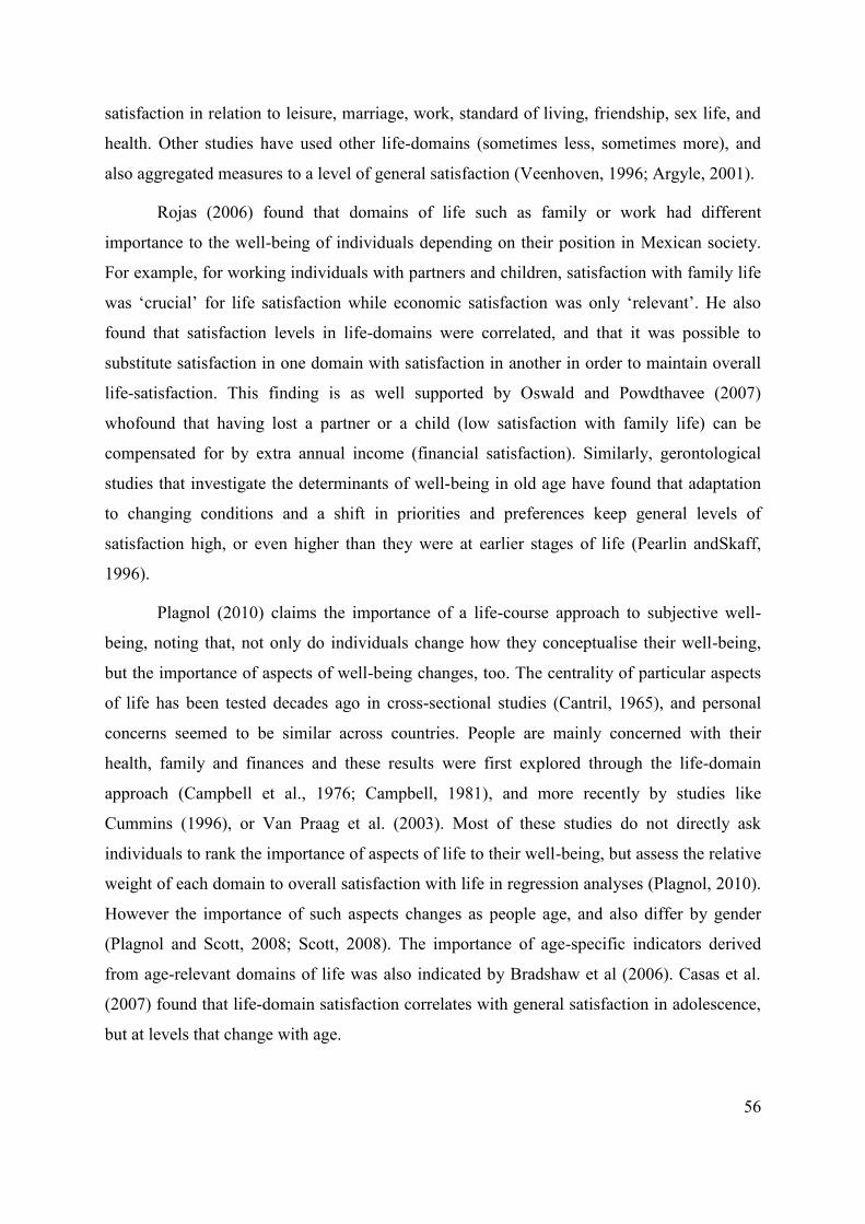
56
satisfaction in relation to leisure, marriage, work, standard of living, friendship, sex life, and
health. Other studies have used other life-domains (sometimes less, sometimes more), and
also aggregated measures to a level of general satisfaction (Veenhoven, 1996; Argyle, 2001).
Rojas (2006) found that domains of life such as family or work had different
importance to the well-being of individuals depending on their position in Mexican society.
For example, for working individuals with partners and children, satisfaction with family life
was ‘crucial’ for life satisfaction while economic satisfaction was only ‘relevant’. He also
found that satisfaction levels in life-domains were correlated, and that it was possible to
substitute satisfaction in one domain with satisfaction in another in order to maintain overall
life-satisfaction. This finding is as well supported by Oswald and Powdthavee (2007)
whofound that having lost a partner or a child (low satisfaction with family life) can be
compensated for by extra annual income (financial satisfaction). Similarly, gerontological
studies that investigate the determinants of well-being in old age have found that adaptation
to changing conditions and a shift in priorities and preferences keep general levels of
satisfaction high, or even higher than they were at earlier stages of life (Pearlin andSkaff,
1996).
Plagnol (2010) claims the importance of a life-course approach to subjective well-
being, noting that, not only do individuals change how they conceptualise their well-being,
but the importance of aspects of well-being changes, too. The centrality of particular aspects
of life has been tested decades ago in cross-sectional studies (Cantril, 1965), and personal
concerns seemed to be similar across countries. People are mainly concerned with their
health, family and finances and these results were first explored through the life-domain
approach (Campbell et al., 1976; Campbell, 1981), and more recently by studies like
Cummins (1996), or Van Praag et al. (2003). Most of these studies do not directly ask
individuals to rank the importance of aspects of life to their well-being, but assess the relative
weight of each domain to overall satisfaction with life in regression analyses (Plagnol, 2010).
However the importance of such aspects changes as people age, and also differ by gender
(Plagnol and Scott, 2008; Scott, 2008). The importance of age-specific indicators derived
from age-relevant domains of life was also indicated by Bradshaw et al (2006). Casas et al.
(2007) found that life-domain satisfaction correlates with general satisfaction in adolescence,
but at levels that change with age.

57
Some events may affect only a few aspects of life, which in turn may affect the
conceptualisation of ‘the good life’ to a greater or lesser extent. However, to understand the
effect of an external event or factor on well-being, it is necessary to assess the individual’s
conceptualisation of well-being (what matters most in life), which will also impact on their
subjective evaluation of well-being (Plagnol, 2010:756-7).
Accordingly, in the analysis of the relationship between subjective well-being and
higher educational achievement, this thesis accounts for conceptual differences in self-
assessed well-being. The literature discussed above leads towards the following questions:
Are domains of life equally important to the subjective well-being of the tertiary-
educated and that of the non-tertiary-educated?
Does the importance of particular domains of life change throughout the life
course?
3.5 The need for research and contribution to knowledge
The higher objective outcomes that are associated with higher levels of education have long
been discussed in the literature (Veenhoven, 1996; Hartog and Oosterbeek, 1998;
Blanchflower, 2001; Headey, Muffels and Wooden, 2004). The tertiary -educated have better
health, better jobs, most often higher pay rates, more wealth and better social networks than
their counterparts with lower levels of education. Therefore the tertiary-educated should
achieve higher utility, or overall well-being (Hickson and Dockery, 2008:3). However, when
material wealth variables are controlled for, a negative relationship emerges between tertiary-
education achievement and subjective well-being. While many studies have identified the
negative relationship between tertiary education and subjective well-being in developed
countries, few have attempted to explore its bases. Hickson and Dockery (2008) and
Dockery(2010) have flagged the need of further investigation of this relationship. There is a
gaparound education and subjective well-being, not only in relation to theory, but also in the
methodological approach (Desjardins, 2008). For example, number of years spent in
education and highest level of education achievement give different results when used in
factor analyses (Desjardins, 2008), indicating some of the weaknesses of the investigation.
Through its methodological and theoretical approaches this study answers the need
for further theoretical and empirical investigation of education and quality of life (Desjardins,
2008; Dockery, 2010). It adds to the scholarly debate in the field of education and subjective

58
well-being in particular, and to the overall discussion of quality of life. The broader
contribution to knowledge of this thesis is discussed in Chapter 10, Section 2 when the
methodological innovations, theoretical implications and policy recommendations are
discussed.
3.6 Conclusion
The purpose of this chapter has been to offer an in-depth review of the bodies of literature
within which the thesis is located. The focus of the thesis is perceived well-being, hence the
studies selected for review are those that have embraced a subjective well-being approach to
individual well-being. Through a critical review of socio-economic and relevant
psychological, medical and gerontological studies, the multidirectional relationship between
subjective well-being, educational achievement, and socio-economic and demographic
variables has been mapped. Relevant methodological approaches to the exploration of
subjective well-being have also been reviewed.
The gap in the literature has been identified and how the thesis participates in the
scholarly debate has been explained. Given the purpose of the thesis, empirical studies have
been the main target of this literature review. As far as possible, reference has been made to
the Australian context but the topic draws on wider perspectives by including international
and cross-national studies of well-being.
The next chapter addresses the methodological approach of the thesis. The operational
research questions that emerged from this review of literature are incorporated in the chapter.
The datasets used to answer the research questions and test the hypotheses are described, and
the advantages and limitations of the methodology are discussed.

59
Chapter 4 The method of study 4.1 Introduction
This thesis is an empirical exploration of the paradox of subjective well-being (SWB) and
tertiary education in Australia. Both objective and subjective outcomes are important to the
assessment of well-being, but subjective well-being is central to the thesis. The analysis
builds on the subjective well-being approach and the life-domain approach discussed in
Chapter 3, Section 3.4.
Longitudinal analysis of a repeated sample of individuals is conventionally preferred
as the best way of capturing the effect of an event, in the case of this thesis, having obtained a
tertiary degree. However, Australian longitudinal data allow for only up to ten consecutive
years, and hence a longitudinal analysis would capture only a short-term effect of education
on well-being. There are also other methodological concerns, such as the ‘instrumentation
bias’ (Baird et al., 2010) that flags the necessity of a ‘refreshed’ and not repeated sample of
respondents each year. This bias is discussed in the final section of this chapter. The thesis
supports the heterogeneity of subjective well-being by higher educational achievement and
explores the subjective well-being of tertiary-educated (TE) and non-tertiary-educated (NTE)
Australians through ‘pre-post intervention’ andwithin- and between-group analyses.
In what follows, data from national representative surveys are analysed in cross-
sectional models. The main body of analysis is conducted using nine waves of data (2001-
2009) from the Household, Income and Labour Dynamics in Australia (HILDA). Information
on a single-item measure for SWB (overall satisfaction with life) and satisfaction with key
domains of life is available, reporting on satisfaction with employment opportunities,
finances, free time, safety, health, home, local community and neighbourhood. An
alternative, multiple-item measure of SWB is calculated in the analysis as the arithmetic
average of the levels of satisfaction with these aspects of life33. The methodological aspects
of the multiple-item calculation are discussed in detail in Chapter 5, Section 5.2 when the
analysis is conducted.
Although there is a possibility of measurement errors resulting from the use of
happiness or satisfaction as measures of SWB, this thesis uses an alternative measure of 33A weighted average is also calculated although, for the ease of understanding and for the purpose of the
present analysis, the arithmetic average is sufficient and preferred (for further discussion of the difference between the two averages, see Rojas, 2004).

60
SWB, happiness with life, from the Australian Survey of Social Attitudes (AuSSA) to
complement findings from the HILDA survey. This comparison is discussed in Appendix C
at the end of the thesis. A comparison with the Personal Well-Being Index (PWI) is also
provided in that appendix.
Data from the HILDA survey is analysed to investigate the SWB and satisfaction with
certain domains of life of the adult population over 25. The SWB of Australians younger than
25 is explored using data from the Longitudinal Survey of Australian Youth (LSAY). In
LSAY, SWB is measured both as a single-item, happiness with life, and through multiple
items, happiness with the following aspects of life: work and study; free time; relationships;
social life; finances; career prospects; future; life at home; standard of living; and home. The
LSAY dataset is preferred for this group of individuals as it addresses youth-specific issues,
which is essential in the conceptualisation of SWB.
The remainder of the chapter is structured into six sections. Section 4.2 discusses the
advantages and limitations of quantitative data analysis in SWB research. Section 4.3
presents the datasets used in the analysis, as well as the steps taken in the analysis of each
dataset. In Section 4.4 the research design is explained. How the operational research
questions that emerged from the review of literature are answered to test the hypotheses of
this thesis is discussed first. Then the life-domain approach and the heterogeneity of SWB,
the methodological approaches employed in this thesis, are explained. Section 4.5 concludes
with a discussion of the biases identified in studies of quality of life, and how this analysis
addresses them.
4.2 Secondary quantitative data analysis
Secondary data in large, longitudinal datasets is often the preferred method of analysts in the
social sciences for capturing past information, change and interactions between factors across
long periods of time. For example, studies of quality of life or well-being traditionally
analyse large sets of data collected at regional, national or global levels such as the British
Household Panel Study (Blanchflower and Oswald 2004; Clark 2007; Baird et al, 2010), the
American General Social Survey (Blanchflower and Oswald 2004), the German Socio-
Economic Panel Survey (Wunder et al. 2009; Baird et al. 2010), the European Social Survey
(Noll, 2006), the European Household Panel Survey (Christoph and Noll, 2003), the

61
Household, Income and Labour Dynamics in Australia (Headey and Wearing 1992; Headey
2010), and the World Values Survey (Veenhoven, 2009).
Although not employed in this thesis, qualitative research methods often provide
valuable information that is not captured by quantitative data. An in-depth understanding of
the human behaviour is often gathered through qualitative research, offering answers to why
and how events happen, rather than when, where, and how often. Newman (2000) compiled a
comprehensive comparison table of quantitative and qualitative research styles: quantitative
research measures objective factors while qualitative research addresses social reality and
cultural meaning; quantitative research focuses on variables while qualitative research
focuses on interactive processes and events; in quantitative research reliability is key while in
qualitative research authenticity is key; quantitative research uses statistical methods to
analyse many cases while the qualitative research undertakes thematic analyses of fewer
subjects (Newman, 2000: 16).
Assessing SWB is a challenging task and there is an on-going debate around ‘the
right’ measure. The concept has both cognitive and affective components (Diener, 1994:
106), and psychologists argue that individuals give different answers to the general question
‘All things considered, how satisfied are you with your life these days?’ depending on
contextual factors such as the time of the day or even the weather. Such issues often result in
problems of validity and reliability in the indicators of self-assessed well-being (von Hoorn,
2007). For such methodological reasons conducting qualitative interviews to explore SWB is
a complex task which necessitates extensive, multi-disciplinary training. Although a
qualitative approach may be valuable to the exploration of SWB by higher educational
achievement, given the time-frame for the completion of this doctoral thesis and resource
constraints, quantitative methods are employed.
The breadth of data available and the savings of time and money are two major
advantages of using secondary data in this research (see also Boslaugh, 2007). The collection
of Australia-wide primary data was beyond the financial possibilities and time frame of this
doctoral project, and the availability of reliable longitudinal data in electronic format allowed
for a considerable amount of time to be allocated to testing hypotheses and models to answer
the research questions posed by this thesis. The largest part of the analysis is conducted using
data from the Household, Income and Labour Dynamics in Australia (HILDA) survey,
restricted to the adult population aged 25 years and older. The purpose of this analysis is to

62
explore the relationship between educational achievement and SWB, hence the adult sample
is confined to individuals who would have reached the tertiary-education completion age. In
addition, the subjective well-being of young people is explored using data from the
Longitudinal Survey of Australian Youth (LSAY).
Although the purpose of these surveys is much broader than the assessment of
individual well-being by highest educational level achieved, both surveys provide
information relevant to the thesis. LSAY inquires about young people’s levels of happiness
with life and domains of life, and HILDA contains a module measuring SWB as satisfaction
with life and satisfaction with areas of life. The Australian adult population also ranked their
happiness in the Australian Survey of Social Attitudes (AuSSA). This information in AuSSA
is also analysed in an attempt to explore the differences between the cognitive measure
(satisfaction) and the affective measure (happiness) of SWB. Results are compared with
those obtained from the analysis of the HILDA data and reported in Appendix C.
The three national datasets are described in the next section: both the data collection
process, and the variables of interest and their descriptive characteristics. The limitations of
these datasets are also discussed. The questionnaires employed by these studies are presented
in Appendix A.
4.3 Secondary data sets
4.3.1 Household, Income and Labour Dynamics in Australia (HILDA) Survey
Data collection
The HILDA survey is a household-based panel study collecting information about ‘economic
and subjective well-being, labour market dynamics and family dynamics’ (Melbourne
Institute, 2010). Both household and individual level data are collected. The survey is
designed and managed by the Melbourne Institute of Applied Economic and Social Research
(University of Melbourne) and was initiated and funded by the Australian Government,
Department of Families, Housing, Community Services and Indigenous Affairs (FaHCSIA).
It began in 2001 and data was collected until 2008 (waves 1 – 8) by the Nielsen Company.
Roy Morgan Research is in charge of collection the data from wave 9 (2009) onwards. This
thesis uses Release 9 of the HILDA data (waves 1 to wave 9). Access was obtained through
the license held by the University of New South Wales and data was accessed and analysed in
SPSS and Stata formats.

63
Respondents to the HILDA survey have been randomly selected and all persons older
than 15 years in eligible households are included and followed for consecutive years. If
individuals change households or form new ones, the new households also enter the survey
and form a ‘refreshed sample’ that adds to the initial sample. Individuals aged 15 and over
from the new household as well become part of the survey, either as a responding person
(completing the entire questionnaire) or as an enumerated person (when only socio-economic
and demographic characteristics are recorded).
The data has been de-identified before release through measures such as withholding
some variables (such as post code), aggregating some variables (such as reporting occupation
at two digit level although was collected at four digit level), or top-coding34variables like age,
income or wealth. Respondent data on demographics such as age, gender, marital status,
geographic location, ethnic background, language spoken at home, family composition,
highest school level or highest qualification obtained, and socio-economic measures such as
wealth, health, income and social attitudes, are available in every wave of the data collection.
Special modules on various topics are at times included, and a comprehensive module on
SWB is present in all waves. Respondents are asked to rank on a scale from 0 to 10 their
levels of satisfaction with life overall, and with eight aspects of life: the home they live in;
employment opportunities; financial situation; safety; feeling part of the local community;
health; neighbourhood; and the amount of free time they have.
Three types of datasets are available for each wave: household data; respondent data;
and enumerated person data. The module inquiring about SWB was completed only by
responding persons, hence the dataset used is the respondents’35. 13,301 respondents
participated in the last wave (Wave 9, 2009), including individuals from new
households(households that were not present in previous waves of data collection), or young
people that reached the eligible age to be in the survey. From these 10,675 (in Wave 9) are
34Top-coding substitutes an average value for all the cases which are equal to or exceed a given threshold. The
substituted value is calculated as the weighted average of the cases subject to top-coding. As a result, the cross-sectional weighted means of the top-coded variable will be the same as the original variable (Source: www.melbourneinstitute.com/hilda/manual)
35Wave 1 (in 2001) has a response rate of 66 per cent and the non-respondents are more likely to live in Sydney, be male or unmarried, born in a non-English speaking country, or aged 20 to 24 or over 65. 7,682 households have been interviewed, with an average of 2.4 people per household resulting into 19,914 people participating in the survey. However 4,787 are ineligible children (under 15) resulting in 13,969 responding individuals. The wave-on-wave attrition rates are highest in waves 2 and 3 (13.2 and 9.6 per cent respectively), falling below 6 per cent for waves 5, 6, and 7 and below 5 per cent for waves 8 and 9.

64
aged 25 years and older, and eligible for the purpose of this analysis.The data is modelled at
individual level.
Following on from this present chapter, Chapter 5 explores the differences in overall
satisfaction and the levels of satisfaction with various domains of life for individuals who
completed tertiary studies and those who did not. ‘What counts’ towards the SWB of the
tertiary-educated and the SWB of the non-tertiary-educated is explored in correlation and
regression analysis in Chapter 6, where the heterogeneity of SWB by higher educational
achievement is explored. Econometric models further investigate how the factors that
influence SWB vary for the tertiary-educated (TE) and the non-tertiary-educated (NTE).
Finally, in Chapter 7, SWB by higher educational achievement is explored in the light of life-
course theory. The econometric models are explained within the respective chapters.
Data description
Table 4.1 summarises the descriptive statistics of the HILDA respondents in 2009.
Information on the entire sample and three sub-samples of the survey is provided. The three
sub-samples are: the adult respondents aged 25 and over; tertiary-educated adult respondents;
and non-tertiary-educated adult respondents. The demographic differences between all
HILDA respondents (Table 4.1-1) and HILDA respondents 25 years and over (Table 4.1-2)
indicate: higher male-to-female ratios among the 15-24-year-olds; higher rates of young
people from Aboriginal and Torres Strait Islander (ATSI)and Culturally and Linguistically
Diverse(CALD) backgrounds; more young people living in major urban areas; and
unsurprisingly, higher rates of single individuals aged 15 – 24 than among the whole
population.
Demographic differences are also apparent between the TE (Table 4.1 – 3) and the
NTE (Table 4.1 – 4). Within the TE sample the ratio of female-to-male respondents is higher
than within the NTE sample, indicating that women have higher university participation rates
than men. The ATSI population is underrepresented in the TE population compared to their
representation in the general population. The proportion of CALD individuals with higher
qualifications is higher than the proportion of CALD respondents without tertiary
qualifications. Almost three-quarters of the TE respondents live in major urban areas, while
just over half of the NTE respondents live in such large metropolitan areas. Not surprisingly,
the TE are slightly younger than the NTE, a consequence of the expansion of tertiary
education participation in the past few decades.

65
Table 4.1 Demographic characteristic of samples in HILDA (per cent)
Demographic characteristics All HILDA respondents (1)
HILDA respondents 25 years and older All 25+
(2) TE (3)
NTE (4)
Gender Male 49.4 47.0 44.5 47.9 Female 50.6 53.0 55.5 52.1 ATSI 3 2.6 1.2 3.1 CALD 16.2 10.1 12.6 9.2 Geographic area Major Urban 65.3 59.7 74.3 54.9 Other Urban 21.2 24.0 14.9 27.0 Rural 13.5 16.2 10.7 18.0 Age group 15-24 18 - - - 25-34 17.5 19.6 26.3 17.4 35-44 17.7 21.7 24.9 20.6 45-55 17.2 22.2 24.3 21.5 55-64 14.3 16.8 14.9 17.4 65-74 8.7 11.0 6.7 12.4 75+ 6.7 8.7 2.8 10.6 Marital Status & Children Single 27.9 12.3 12.6 12.2 Married 57.7 66.2 72.6 64.1 Separated 2.6 3.9 3.7 3.9 Divorced 7 11.0 8.8 11.7 Widowed 4.7 6.6 2.4 8.0 Children 61.2 75.6 66.2 78.7 Long term health or disability 23.2 26.7 16.5 30.1 Employment Status Employed 63.5 64.2 79.4 59.1 Unemployed 3.6 2.3 1.9 2.5 NILF 32.9 33.5 18.6 38.4 Education level Masters or PhD 3.5 4.5 18.0 - Grad diploma/certificate 4.7 6.1 24.7 - Bachelor or Hons 12.9 14.2 57.3 - Non-tertiary 78.9 75.2 - 100 N 13,301 10,675 2,645 8,030 Source: HILDA, 2009, weighted sample; total N from un-weighted sample.
A higher percentage of TE individuals are married, although it is worthy of note that a
higher percentage of NTE respondents have children36. The descriptive statistics of the two
sub-samples also indicate that fewer TE respondents have a long-term illness or disability,
consistent with the literature reviewed in Chapter 3, Section 3.3.1. Predictably, a higher share
of the TE than the NTE is employed. Population weights are used with each year of data to
ensure that results from the analysis are representative for the general Australian population.
36 Respondents were directly asked to state their marital status and whether they currently had children.

66
4.3.2 Longitudinal Survey of Australian Youth (LSAY)
Data collection
The Longitudinal Survey of Australian Youth (LSAY) is the most comprehensive research
study on young people in Australia, managed and funded by the Australian Government
Department of Education, Employment and Workplace Relations (DEEWR) with support
from local governments. The project is ongoing, and the Wallis Consulting Group has been
collecting the data by computer-assisted telephone interviewing (CATI) since 1995. Until
2003, young people were randomly selected from schools across all Australian states and
territories. Since 2003 however, survey participants have been selected from amongst the
young people participating in the Australian component of the Organisation for Economic
Co-operation and Development’s (OECD’s) Programme for International Student
Assessment (PISA) survey. Young people enter the survey when they turn 15 (or, prior to
2003 in Year 9), and are contacted annually for the next ten consecutive years for follow-up
interviews. Groups of students that enter the survey at the same time (when they turn 15) are
known as a ‘cohort’. There are five cohorts: year 1995 cohort (Y95), year 1998 cohort (Y98),
year 2003 cohort (Y03), year 2006 cohort (Y06) and year 2009 cohort (Y09). Each cohort
initially consists of over 10,000 students. Although attrition rates are relatively high, attrition
weights are provided and used in this analysis. De-identified data is available on request from
the Australian Social Science Data Archive (ASSDA) at the Australian National University
(ANU) in Canberra. For the purpose of the thesis, data were obtained and analysed in SPSS
format.
Data description
The survey tracks young people as they move from school to further education, work and
other destinations, and a variety of demographic and socio-economic characteristics are
collected. Information on family, friends, social connectedness, physical and mental health,
school performance, subjects studied at school, plans to complete school, plans for further
education, work history, frequency of recreational activities, aspirations and social attitudes,
and happiness with life overall and with various aspects of life, are just few of the aspects
explored by the LSAY survey.
The Y95, Y98 and Y06 cohorts are of interest to this analysis. The Y95 and Y06
cohort data are analysed to explore school completion and tertiary-education participation in
the light of the capabilities approach. The Y98 cohort provides the most recent information

67
on young people whohave finished their transition from school to work. In Chapter 9 this
cohort is explored longitudinally in order to investigate the differences between the TE and
the NTE young people. The Y95 cohort consists of a random sample of 13,613 Year 9
students with an average age of 14.5 years at the time. The Y98 cohort consists of 14, 117
students with an average age of 14.5 years at that time. 14,170 Australian students were
selected in 2006 to participate in the PISA conducted by the OECD. The average age in 2006
was 15.7 years, and these students became the LSAY Y06 cohort37. All members of a cohort
are contacted for annual follow-ups and the condition for remaining in the survey is to miss
no more than one wave of data collection. A disadvantage of the LSAY survey is the high
attrition rates. Table 4.2 summarises the sample sizes and annual attrition rates recorded
within each cohort throughout the years of data collection.
Table 4.2 Sample size and response rates Y95, Y98 and Y06 LSAY cohorts
Interview period (year)
Y1995 Y1998 Y2006 Sample size Response rate Sample size Response rate Sample size Response rate
1 13613 100 14117 100 14170 100 2 9837 72.3 9289 65.8 9353 66.0 3 10307 75.7 9548 67.6 8380 59.1 4 9738 71.5 8777 62.2 7299 51.5 5 8783 64.5 7762 55.0 6 7889 58.0 6905 48.9 7 6876 50.5 5979 42.4 8 6095 44.8 5356 37.9 9 5354 39.3 4729 33.5 10 4660 34.2 4210 29.8 11 4233 31.1 3859 27.3 12 3,914 28.8 3596 25.5 Source: NCVER
Consistent with the recommendation of the National Centre for Vocational Education
Research (NCVER),two weighting procedures have been applied to the LSAY data in this
analysis, to ensure that it accurately represents the population aged 15 in the first year of
collection. The first procedure involves sample weights which ensure that the sample matches
the population from which it was drawn; the second procedure involves attrition weights
which allow for the rather high attrition rates that characterise the LSAY survey. These
weights are based on the overall achievement quartiles and gender, and reweighted to wave
37 The Y06 cohort students were slightly older during their first wave of interviews in 2006 than the young
people beginning their interviews in 1995. All young people in the Y95 cohort were in school Year 9 in 1995, while the Y06 cohort young people were in school Year 10. The waves are not linearly comparable and data from the first wave of the Y06 cohort is compared to the data from the second wave of the Y95 cohort to match characteristics like age or school year.

68
one (NCVER 2006). The two weights are combined into a final weight that both accounts for
attrition and balances the sample to the population size. These final weights have been used
in all LSAY technical reports and are also used in the analysis presented in this thesis.
4.3.3 Australian Survey of Social Attitudes (AuSSA)
The Australian Survey of Social Attitudes (AuSSA) is also used in the thesis to explore
biases that occur from the use of affective (happiness) and cognitive (satisfaction) measures
of well-being. Managed by the Australian Demographic and Social Research Institute
(ADSRI) at the ANU, the AuSSA is a biennial survey of the social attitudes and behaviour of
Australians. AuSSA was first conducted in 2003. It is a mail survey and approximately 4000
Australians aged 18 and above are randomly selected from the Electoral Roll at each round.
To maintain the confidentiality of the information provided, the postcode variable is
permanently embargoed.
The 2009 survey has two modules (AuSSA-A and AuSSA-B). Module A was sent to
a sample of 5,002 individuals and module B to 5,002. The response rates were 37 per cent for
AuSSA-A and 33 per cent for AuSSA-B. This thesis uses data from the AuSSA-A, which
contained the module for the International Social Survey Program (ISSP) 2008 as well as
information on happiness. Because the sample is biased – more women than men, and more
of the highly-educated and of older people than the general population – the sample is
weighted to have same properties as the Australian Bureau of Statistics (ABS) Census 2006
data.
The first question in Section A of the 2009 AuSSA-A questionnaire inquires about the
general level of happiness, with answers ranked as very happy, fairly happy, not very happy
and not at all happy. Section J asks about the personal background of the respondent –gender,
year of birth, years of schooling, highest level of education achieved, current occupation,
marital status and family background, ancestry and more.
Although the data provided by the AuSSA is not longitudinal, that is, the survey does
not follow individuals across waves of data collection, the data provided by this survey is
valuable in more than one respect. Firstly, it is representative of all Australians, as individuals
have been randomly selected from all regions of Australia and across all age groups (18-year-
olds and above). Secondly, the AuSSA survey allows for the computation of an alternative
measure of SWB (happiness) to compare with the levels of satisfaction derived from the

69
HILDA survey. The results of this analysis of overall happiness, and the comparison with
overall satisfaction with life, are included in Appendix C at the end of the thesis.
4.4 The design of the analysis
The framework of the thesis was developed in Chapter 2 and three hypotheses were
formulated. Chapter 3 provided a critique of the SWB literature in the light of the paradox of
SWB and tertiary education. The following research questions emerged from the literature
reviewed:
Are the TE less satisfied with aspects of their lives than the NTE?
Are the TE less satisfied with their lives overall than the NTE?
Are domains of life equally important to the SWB of the TE and the NTE?
Does the importance of domains of life change throughout the life course?
Do demographic and socio-economic factors affect the SWB of the TE and NTE
to the same extent?
Is there a paradox of SWB and tertiary education in Australia?
These operational research questions are addressed empirically. Changes in levels of
satisfaction with certain areas of life and in overall satisfaction with life between 2001 and
2009 are first explored using data from the HILDA survey. Within-group and between-group
comparisons of means are conducted. The within-group comparison of means explores how
the levels of overall satisfaction with life (SWB) and satisfaction with domains of life have
changed in the past decade for tertiary-educated and non-tertiary-educated Australians. The
within-group focus is the change within each group of individuals, that is, the change in
satisfaction for the TE between 2001 and 2009, and the change in satisfaction for the NTE
between 2001 and 2009. The between-group comparison investigates the differences between
the TE and the NTE with respect to their levels of overall satisfactionon the one hand, and
their levels of satisfaction with certain areas of life on the other. In this instance, the focus is
on the differences between the two groups, the TE and the NTE, occurring across time, rather
than on the differences occurring within each group.
This comparative analysis gives a first indication of how Australians with different
levels of education compare in terms of overall satisfaction with life and satisfaction with
certain domains of life, addressing the first two operational research questions. The results

70
indicate that in 2009 the tertiary-educatedhad similar levels of subjective well-beingto the
non-tertiary-educated, pointing towards aninitial resolution of the paradox of SWB and
tertiary education in Australia. However, when an aggregate measure of SWB is calculated as
the average of the levels of satisfaction with key areas of life, the tertiary-educated are found
to be significantly more satisfied with their lives than the non-tertiary-educated. The paradox
of SWB and tertiary educational achievement is both confirmed and refuted through this
comparison analysis, and these diverging results flag the necessity for further exploration of
the relationship between subjective well-being and tertiary-educational achievement.
Building on the theoretical framework developed in Chapter 2, this thesis supports the
heterogeneous nature of SWB by higher educational achievement and age. The next stages of
the analysis explore the heterogeneity of SBW by higher educational achievement, first
through a life-domain approach, and later from a life-course perspective. For this purpose,
correlation analyses of data from the 2001 and the 2009 HILDA surveys explored the
question of whether particular domains of life were equally important to the SWB of the TE
and the NTE, and how these correlations might have changed over the past decade. The
factors that influence the SWB and satisfaction with aspects of life of the TE and the NTE are
then explored in regression analysis, further testing the heterogeneous nature of SWB. Age is
also an important factor in explaining perceptions of well-being, and for this reason the
heterogeneity of SWB by tertiary-educational achievement and stage of the life-course is
explored in Chapter 8.
The results of both the single-item and the multiple-item measures of SWB are
explored, and the paradox of SWB and higher-educational achievement in Australia is
reassessed. Both the life-domain approach and the heterogeneity approach to SWB are central
to the design of the analysis, and are discussed below.
4.4.1 Life-domain approach and the heterogeneity of subjective well-being
The life-domain approach (Campbell et al., 1976; Campbell, 1981) is a bottom-up approach
to exploring determinants of well-being. It assumes that overall well-being is driven by the
levels of satisfaction with various domains of life.
Whether the relationship between life satisfaction in general and satisfaction with
domains of life is additive (Moller and Saris, 2001; Cummins, 2010), or whether the
relationship is instead semi-logarithmic or logarithmic, or whether constant elasticity of

71
substitution can be applied, is another debate in the assessment of SWB (Rojas, 2006). Using
Mexican data, Rojas (2006) found that general life satisfaction is not a weighted average of
life-domain satisfaction, and that the relationship between them is rather complex. Different
weights have been found to apply to domains of life according to individual characteristics.
For example, for working individuals with partners and children, satisfaction with family life
is ‘crucial’ for life satisfaction, followed by satisfaction with health, personal life and job
ranked as ‘important’. For the same group of people economic satisfaction is only ‘relevant’
while friendships and community domains become ‘irrelevant’ (Rojas, 2006:490-491). This
suggests that some groups of individuals are different and the phenomenon of the various
perceptions of well-being has been discussed as the ‘heterogeneity’ of the respective groups
(Rojas, 2006).
Furthermore, drawing on the theoretical framework built in Chapter 2, the central
premise of the thesis is that what makes the TE satisfied does not satisfy the NTE to the same
extent. This phenomenon is discussed in this thesis as the ‘heterogeneity of SWB by tertiary-
educational achievement’. For these reasons, a regression analysis with semi-logarithmic
specifications (for a comparison of this model with other possible models – see Rojas, 2006)
explores the influence of satisfaction with aspects of life on overall satisfaction with life for
the TE and the NTE. The heterogeneity of SWB and tertiary-educational achievement is
assessed through this analysis. If the levels of satisfaction with domains of life have a similar
influence on overall satisfaction with life for the TE and the NTE, it can be concluded that
areas of life have the same importance for individuals from the two groups, refuting the
hypothesis of the heterogeneity of SWB by tertiary-educational achievement. Whether or not
this is the case, whether in fact the TE and NTE have different concepts of ‘what counts’ for
their well-being, is explored in Chapter 6.
The life-domain approach also assumes that external factors influence only some and
not all aspects of life. For this reason, socio-economic and demographic factors (such as
marital status, income group, employment status, or demographics like gender, age group, or
ethnic background, factors traditionally assessed in studies of subjective well-being) that can
affect satisfaction with life and satisfaction with domains of life are also explored. Whether
the influence of these factors is the same for the TE and the NTE is explored, allowing
conclusions to be drawn about whether ‘what makes the good life’ varies by level of

72
education. The results and detailed methodological specifications of the models are discussed
in Chapter 7.
The life-domain approach and the bottom-up analysis of SWB are hence identified as
suitable methodologies for the exploration of the paradox of SWB and tertiary education in
Australia.
4.4.2 Specifications of the analysis and its limitations
When the purpose is to observe changes across individuals due to an intervention program or
an event, time-series data analysis is preferred (Wooldridge, 2006):
Panel data sets are very useful for policy analysis and, in particular, program evaluation. In the simplest program evaluation setup, a sample of individuals, firms, cities and so on is obtained in the first time period. Some of these units, those in the treatment group, then take part in a particular program in a later time period; the ones that do not are the control group.
(Wooldridge, 2006:467)
However, although the effect of an event (completing tertiary education) is what this
thesis seeks to explore, a pre-post intervention analysis is not appropriate here. The following
scenario gives reasons for this decision: the first time-period (pre-intervention) is 2001, the
first year of the HILDA data collection, and the post-intervention period is the last year of
data collection, 2009. Obtaining a tertiary qualification (bachelor level and above) is the
intervention. The first problem is that individuals who already had a tertiary qualification in
2001 would be omitted from the analysis, as they had already ‘received the intervention’.
Secondly, the year of tertiary-qualification completion would vary across individuals within
the remaining sample, as they could have completed a tertiary qualification at any point
between 2002 and 2009. Thirdly, even if a control for the year of completion were to be
introduced, for some individuals the effect of having completed tertiary qualifications would
be a short-term effect (e.g. for those who have completed in between 2005 and 2009), while
there would be a medium- to long-term effect for others who had completed tertiary
education four or more years prior to the year of analysis. Accounting for the short- and long-
term effects would reduce the sample size, presenting the analysis with further difficulties.
For these reasons, a ‘before-after intervention’, longitudinal analysis to isolate the
effect of tertiary education completion on satisfaction with life is not appropriate given the

73
data available for analysis. Furthermore, a repeated sample of respondents is necessary to
observe the change in time (Wooldridge, 2007). However, Baird et al. (2010) argue that there
is a participation bias in repeated cross-sectional analyses of SWB: being asked each year to
subjectively evaluate their lives, individuals may become more reflective and change their
attitudes each year, their following year’s answer being influenced by their participation in
the survey the year before. For this reason, Baird et al. (2010) suggest that refreshed samples
in unbalanced longitudinal panels should be used to control for this bias. This bias is
addressed in the context of the HILDA survey and results are reported in Appendix Cat the
end of the thesis. The analysis conducted throughout the thesis uses a refreshed longitudinal
sample of respondents.
The analysis employed by this thesis divides the respondent sample into tertiary-
educated (individuals who have completed studies at bachelor levels and above) and non-
tertiary-educated individuals. All nine waves of HILDA data are initially considered, and all
respondents (as opposed to the repeated sample only) are included to compare the change in
levels of satisfaction with life and of satisfaction with domains of life for the TE and the
NTE, between 2001 and 2009. This comparative analysis is conducted in Chapter 5.
In order to test the heterogeneity of SWB by tertiary-educational achievement
discussed in the subsection above, an in-depth analysis is conducted of the influence on
overall satisfaction of satisfaction with domains of life and of socio-economic and
demographic factors. The analysis is done separately for the TE and the NTE, using 2009
HILDA data. The goal of this cross-sectional analysis is to explore whether the determinants
of SWB are the same for the two groups. The same cross-sectional analysis is repeated using
2001 data and the results of this analysis are compared with the results from 2009. The
purpose is to explore through a time-series cross-sectional comparison how determinants of
well-being have changed between 2001 and 2009 for the TE and the NTE. A pooled cross-
sectional analysis is the traditional method for exploring such changes in impact factors
across periods of time. Dummy variables are usually included for each time period, and
interaction terms created to differentiate between the impact of each factor in period 1 and
period 2 respectively. However, in this analysis, the dependent variable (satisfaction with
life) is conceptually different not only in the case of the TE and NTE (i.e. SWB is
heterogeneous by higher educational achievement), but also in each year of assessment.
Chapter 6, Section 6.2, shows that correlations between the levels of satisfaction with

74
domains of life and the levels of overall satisfaction are different for 2001 and 2009, and
these correlations are also different for the tertiary-educated and the non-tertiary-educated.
Chapter 6 concludes that SWB is heterogeneous by higher-educational achievement. This
chapter also offers an empirical explanation for the inappropriateness of a pooled-cross-
sectional analysis.
4.5 Methodological biases in quality of life research
Well-being studies have traditionally undertaken empirical analyses of large regional,
national or international datasets38. These studies include those investigating the determinants
of objective or subjective well-being such as income (Easterlin, 1974; Diener et al., 1999;
Veenhoven and Hagerty, 2006), gender (Headey and Wearing, 1992; Hartog and Oosterbeek,
1997; Inglehart et al., 2002), marital status (Diener et al, 1995; Masterkaasa, 1994; Gerdtham
and Johannesson, 2001) and health (Gerdtham and Johannesson, 2001; Dolan et al., 2007), as
well as those investigating the relationship between subjective and objective well-being
(Wilson, 1967), and the relationship between satisfaction with areas of life and overall
satisfaction with life (Diener, 1984; Veenhoven, 1988; Cummins, 1996; Headey and
Wearing, 1992; Argyle, 2001; Moller and Saris, 2001; Rojas, 2006; Cummins, 2010).
However many studies have fallen victim to various biases of age, cohort effects or
instrumentation effects. Some of the possible biases identified in well-being research are
listed below. Whether the analysis in this thesis addresses them, and how it does so, is also
explained.
1. Age group bias.
Many researchers included in the analysis of determinants of SWB continuous or dummy
variables for age. Most studies conclude either that SWB does not change with age, or that
there is a U-shaped relationship between age and SWB39. However, very few studies have
explored this relationship further. Plagnol (2010), however, argues that perceptions of well-
being change with age, and that what makes the ‘good life’ can be a function of aspirations
and roles individuals play at different points in life. Such discrepancies in how people define
their well-being are addressed in the thesis through an analysis of SWB by a derived variable
38For a list of some of these surveys see Section 4.3.
39 For reference studies see Chapter 3.6.

75
of age; well-being is analysed at four stages of life: emerging adulthood, early adulthood,
middle adulthood and late adulthood (Elder, 1974). Chapter 7 is entirely dedicated to the
analysis of SWB through a life-course approach.
2. Cohort bias.
The times in which individuals are born can have a unique effect on their attitudes to life
through specific historical events characteristic of their generation alone such as the Great
Depression, the Cold War or the onset of the internet. People born in times of prosperity can
be prone to assessing their lives as good, while those born and brought up under harsh socio-
economic or political conditions can tend to understate their well-being (Baird et al., 2010).
For example, one of the few longitudinal studies of quality of life and educational
achievement (Hartog and Oosterbeek, 1998) investigated data collected over 40 years starting
when respondents were 12. While valuable because it allows the observation of longitudinal
change, the bias of a population that is born in the 1940s can be strong enough for the reader
to argue that the results are not representative for current generations.
Respondents to the HILDA survey were born across seven decades (respondents are
aged 18 to 95), hence the overall statistics of the sample are not biased towards a single
generation. Such data make the results less susceptible to generational biases. However,
individuals that changed their status from NTE to TE between 2001 and 2009 are likely to be
in the same age bracket (that is, age 24 to 30), mature-age education being infrequent.
Nevertheless, including all respondents in the analysis balances the data to represent as much
as possible the general population. Furthermore, refreshed samples40 (new respondents) are
used with each wave to eliminate the possibility of an ageing repeated sample of respondents.
3. The centrality of life-domains across the life-course or ‘Focusing effect’ (Plagnol, 2010).
Many studies, including some of those using Australian data (Headey and Warren, 2008;
Cummins, 2010) have found a U-shaped relationship between satisfaction with life overall
and age. However, the relationships between age and satisfaction with domains of life are not
always significant or U-shaped (Cummins, 2002), indicating that individuals have different
appreciations of aspects of life, and of life overall across the life-course. The centrality of 40 Opposed to a repeated sample that would suffer an ageing effect over 9 years of survey, this analysis includes
new survey respondents each year, i.e. a refreshed sample (for clarifications around the use of refreshed rather than repeated samples see Baird et al., 2010).

76
different areas of life changes with individual characteristics such as marital status or the
presence of children (Rojas, 2006). Plagnol (2010) argues the necessity to assess the
importance of life domains to overall well-being, and then assess the impact of external
factors.
This thinking is transposed to the analysis of SWB by higher educational achievement
in Chapter 6, when the influence of satisfaction with domains of life on SWB is explored
first, and then the ways in which external factors interact with SWB and satisfaction with
domains of life are investigated.
How Australians conceptualise their well-being is taken from the HILDA survey.
Respondents are asked to rank their satisfaction with various aspects of life and life overall,
making this survey valuable to the evaluation of SWB through both a life-course approach
and a life domain approach. Furthermore it is possible to differentiate between individuals by
highest level of education attained, allowing an investigation into how the importance of
particular aspects of life changes with age for the TE and NTE, and how the two groups
changed between 2001 and 2009. This latter item is addressed in Section 8.3.
4. ‘Instrumentation biases’ (Baird 2010) – the use of longitudinal data without refreshed
samples.
Baird et al. (2010) assessed SWB in two European countries using the British Household
Panel Study (BHPS) and the German Socio-Economic Survey (GSOEP). They found that in
Germany there was a strong ‘instrumentation bias’, by which they implied that having
participated in the survey in fact influenced the respondents’ lives and how they reported
their well-being the following year. To control for such instrumentation bias Baird et al
(2010) recommend that results from longitudinal repeated survey samples be compared with
results generated by a ‘refreshed’ sample of individuals that would answer each wave of the
survey for the first time. If the differences between the two are statistically significant then it
is advisable to use a refreshed sample, even in the data analysis of two or more periods.
Respondents to the HILDA survey are interviewed each year and followed if they
change house or form new households (i.e. the survey follows the individual not necessarily
the household).Furthermore, all individuals of the new household, if aged 15 or older, join the
survey. These new respondents, and those from the old households who have just turned
15,represent the refreshed sample. Their answers are analysed and compared with those of

77
the repeated sample to investigate whether instrumentation effects such as those found by
Baird et al (2010) alter the analysis of well-being in Australia. The calculations are presented
in Appendix C, section 1.
5. Differences between subjective and objective levels of well-being.
While many studies argue they have identified the determinants of well-being or who is more
likely to be happy, it is important to indicate ‘which quality of life’ or well-being the study
refers to (Schuessler and Fisher, 1985; Farquhar, 1995), as some studies investigate for
example the health-related quality of life, only refer to it as ‘quality of life’, creating
confusion for readers from other fields (Farquhar, 1995).
After a clear indication is made as to ‘which quality of life’ the study investigates, it is
important to differentiate between objective and subjective well-being (Noll, 2001;
Veenhoven 1999), to understand how the self-assessed subjective well-being and the
objective well-being interact and generate overall quality of life (Haas, 1999; Noll, 2000;
Veenhoven, 1999, 2009).
These conceptual differences are acknowledged by this thesis. However, the objective
well-being is outside the purpose of this analysis. The focus is on subjective well-being and
the intentions of the thesis (to assess the relationship between tertiary education achievements
and subjective well-being) have been made most clear in Section 3.2 when the working
definition of SWB was formulated.
6. Potential differences between subjective well-being assessed as ‘satisfaction’ and SWB
assessed as ‘happiness’
The debate around the terminology and measures of subjective well-being has been addressed
in Chapter 3. The distinction between ‘happiness’ and ‘satisfaction’ originates in the field of
psychology where they are defined as the affective and cognitive dimensions of wellbeing
respectively (Argyle, 1987; Diener, 1984).
Satisfaction with life is assessed using HILDA and the main body of analysis draws
on this survey. However, overall happiness is also calculated using the Australian Survey of
Social Attitudes. While the simplicity of the AuSSA survey does not allow for complex
manipulations, the simple comparison of the levels of satisfaction and those of happiness
78
across the general population is an indicator of the conceptual differences that can occur due
to the two different measures. This comparison is presented in Appendix C. At that time, two
measures of SWB using HILDA data (overall satisfaction and satisfaction with life), the
measure of SWB using AuSSA (happiness), and the Personal Well-Being Index (PWI) are
also compared.
4.6 Conclusion
The thesis addresses the necessity for theory formulation and empirical analysis of the
relationship between education and subjective well-being, discussed amongst others by
Desjardins(2008). National Australian data is explored in a life-domain approach and the
heterogeneity of SWB by higher educational achievement is tested. The research aim, the
theory and approaches to concepts place this thesis in the field of quantitative social science
research.
This chapter has discussed the methodological approaches, including alternative
measures of SWB, and introduced the data sets used in the analysis. The advantages and
limitations of secondary data analysis have been addressed. The design of the analysis has
been explained. Finally, the methodological biases that often become a concern in quality of
life research and how they are controlled for in the analysis has been discussed.
The next chapter is the first chapter of analysis and results. The chapter is a time-
series cross-sectional exploration of the paradox of subjective well-being and tertiary
education and various measures of subjective well-being are compared. The first hypothesis
of the thesis is tested in this chapter.

79
Chapter 5 Findings: Satisfaction with life and
satisfaction with domains of life
5.1 Plan of the chapter
This is the first chapter of analysis and results. As theorised in Chapter 2 and supported by
the literature reviewed in Chapter 3, the heterogeneity of SWB by higher educational
achievement is supported in this thesis. For this reason the analysis in this chapter is
structured to address separately the levels of satisfaction of the tertiary-educated and non-
tertiary-educated.
The chapter is structured in six sections. The second section introduces the hypothesis
that is tested in this chapter, and the methodological approach that is employed for this
purpose. Section 5.3 compares the change in overall satisfaction with life and the levels of
satisfaction with domains of life between 2001 and 2009. The purpose is to investigate if the
tertiary-educated and the non-tertiary-educated have experienced the same changes in overall
satisfaction and in satisfaction with life domains of life across the nine years of data analysed.
Between-group and within-group changes are explored. In Section 5.4 an aggregate measure
of subjective well-being is also calculated as the arithmetic average of the levels of
satisfaction with domains of life. Satisfaction with life is explored through a life-domain
approach.
5.2 Introduction to the analysis
The first hypothesis of the thesis examines the existence of the paradox of SWB and tertiary
education in Australia (hereafter referred to at times as ‘the paradox’) and is tested in this
chapter:
H 1. The tertiary-educated a) are more satisfied with aspects of life and,
b) are more satisfied with life overall.
The methodological approach developed in Chapter 4 discussed the application of the
subjective well-being approach,41 life-domain approach,42 and heterogeneity approach to the
41 SWB approach refers to the assessment of individual well-being through a direct question asking the
individual to rank their happiness or satisfaction with life (e.g. How happy are you these days? How satisfied are you with your life overall?)

80
thesis. These approaches are employed in this chapter, and both overall satisfaction with life
and satisfaction with domains of life are explored. An aggregate measure of satisfaction is
also calculated as the average of the levels of satisfaction with key domains of life.
The chapter focuses on the differences in the levels of satisfaction with life and
aspects of life of the tertiary-educated (TE) and not tertiary-educated (NTE) Australians. An
individual is flagged as TE if at the time of the survey s/he had completed a tertiary
qualification at Bachelor level or above (i.e. Bachelor, Masters, or Doctorate). Individuals
with other qualifications, including post-secondary but not tertiary, are flagged as NTE. The
analysis is not confined to a traditional approach of exploring factors that impact on SWB in
multivariate regressions. Instead, the differences between the SWB of TE and the SWB of
NTE are explored through within-group and between-group analyses. The theoretical and
methodological reasons behind the choice of this analysis were discussed in Chapter 2,
Section 2.3 and in Chapter 4, Section 4.4 respectively. The specifications of the econometric
models are explained in Section 5.2.
Nine waves of data (2001 to 2009 inclusive) from the HILDA survey are analysed to
investigate the changes in overall satisfaction with life and satisfaction with domains of life
for the TE and NTE Australians. The interest is not in individuals per se, but in the two sub-
populations, hence individuals are allowed to roam between the groups.43 For example, while
in 2001 one person may be in the NTE group, by 2009 they may have completed a tertiary
qualification and moved to the TE group. The moment that the tertiary qualification is
obtained is not of interest because such control would only capture short-term effects. The
goal of the chapter is to explore how the SWB of individuals in the TE and NTE groups has
changed over time, and how the two groups compare to each other.44
42 The life-domain approach assesses subjective well-being as a function of satisfaction or happiness with
aspects of life. A linear relationship is most of the time assumed (Rojas, 2004) and the domains of life assessed are selected through either factor analysis, availability or based on the research goals.
43 Because only a short impact of having obtained a tertiary qualification can be calculated (data is only available between 2001 and 2009), the analysis is conducted not at individual level but at group level, differentiating between tertiary educated and non-tertiary educated. The members of these groups however are not held constant (it is not a repeated sample), hence some individuals may obtain their degree between 2001 and 2009, changing from NTE group to TE.
44 It was explained in Chapter 4 Methodological approach that in a perfect scenario longitudinal data that would allow following individuals across longer periods of time is generally preferred to assess change in time. This would allow to explore the effect of education of SWB in a pre – post intervention model. Given the data is available only for 9 years, only a short-term effect of education would be captured, hence the interest is not in individuals, but in exploring differences between groups of individuals.

81
Refreshed samples are used with population weights. The main reason for not having
used a repeated sample (individuals that answered each wave of the survey) is to avoid a
participation bias (explained earlier in Chapter 4, Section 4.4). The weaknesses of an analysis
using a repeated sample are discussed in Appendix C at the end of the thesis. Only
respondents aged 25 or older are included in the analysis in Chapters 5-8, otherwise the non-
tertiary population would include young people who would not have had the chance to obtain
a tertiary degree, due first of all, to their age. The SWB of young people is separately
discussed in Chapter 9.
5.3 Changes in satisfaction between 2001 and 2009
5.3.1 Changes in overall satisfaction with life
In the HILDA survey, SWB is assessed as overall satisfaction with life. Respondents
answered the generic question, ‘All things considered, how satisfied are you with your life
these days?’ and ranked their overall satisfaction with life on a 0 to 10 scale, with 0 being
least satisfied and 10 most satisfied. The changes in mean levels of SWB between 2001 and
2009 are summarised in Table 5.1 and are graphically represented in Fig.5.1. Error bars have
been plotted in SPSS to explore whether the differences between the SWB of TE and NTE
(Table 5.1) are statistically significant.45 The econometric convention is that if the error bars
overlap the difference between the items that are being compared is not statistically
significant. However, the converse is not always true. If the error bars plotted for the means
of two independent samples do not overlap, an unpaired t-test is necessary to test the
significance level of the difference between the two means46 (Wooldridge, 2006). For this
reason in Table 5.1 to Table 5.10, the significance level is also noted. The convention is: ***
for p-value between .001 and .005; ** for p-value between .005 and .01; and * for p-value
between .01 and .05. For clarity, these p-values are discussed when thestatistical significance
of the differences graphed in Fig.5.1 to Fig. 5.10 are not clear, that is, when the error bars do
not overlap indicating that the difference of means can be either statistically significant or not
significant. When error bars overlap, as mentioned above, the difference between the two
groups is not statistically significant.
45 See for example Andy P. Field Discovering Statistics Using SPSS for the use of error bars in SPSS to explore
the statistical significance of difference between groups (Field, 2009:103-120).
46 If the p-value obtained from the t-test is less than 0.05 then the difference between the means is statistically significant (Wooldrwidge, 2006).

82
Table 5.1 Mean levels of satisfaction with life (SWB)
Year NTE TE ALL Difference1
2001 7.96 7.78 7.92 -0.18***
2002 7.86 7.71 7.83 -0.15***
2003 7.97 7.77 7.92 -0.2***
2004 7.92 7.82 7.9 -0.1***
2005 7.87 7.78 7.85 -0.09***
2006 7.82 7.76 7.81 -0.06
2007 7.82 7.73 7.8 -0.09
2008 7.84 7.79 7.82 -0.05
2009 7.78 7.82 7.79 0.04
Difference 2009 -20012
-0.18*** 0.04
Source: author’s calculations using HILDA, 2001-2009, individuals age 25 years and older. Person weights were used. N=10,675.
1. Independent sample t-tests (2-tailed) have been run for each year data to check the statistical significance of the difference between the levels of satisfaction reported by the tertiary-educated and the non-tertiary-educated in the respective year. The statistical significance decreases as the p-value increases. If p-value is between .001 - .005, then the difference of means is highly significant and noted as ***. If the p-value from the t-test is between .005 - .01, the significance is noted as ** and if between .01-.05, the notation is *. If the p-value is greater than .05 the results are not statistically significant. Only statistically significant results are noted.
2. The statistical significance of the difference between the mean level of satisfaction with life in 2009 and in 2001 (between the first and last year of data collection) was tested through an independent sample t-test (2-tailed). P-value <.005 indicates the decrease in the mean SWB of non-tertiary-educated between 2001 and 2009 is statistically significant and a p-value >.05 suggests the difference in the levels of satisfaction in 2009 and 2001 is not statistically significant for the tertiary-educated
Fig. 5. 1Overall satisfaction with life (SWB) 2001 – 2009 by education level
Source: author’s calculations using HILDA, 2001 – 2009
7.4
7.5
7.6
7.7
7.8
7.9
8
8.1
2001 2002 2003 2004 2005 2006 2007 2008 2009
Sati
sfac
tio
n le
vel
NTE
TE
Total

83
Between-group and within-group changes are discussed. Between-group changes
confirm that between 2001 and 2005 there was a negative relationship between higher
educational achievement and SWB (as claimed in the literature), and the tertiary-educated
were significantly less satisfied with their lives than the non-tertiary-educated (p<.05).
However, throughout the next 5 years (from 2006 until 2009) the difference between the two
groups lost statistical significance (p>.05, or error bars overlap, see Fig.5.1).In 2009 the SWB
of the tertiary-educated became higher than the SWB of the non-tertiary-educated, but this
difference is not statistically significant. Changes within the two groups are explored next.
Satisfaction with life increased for the tertiary-educated between 2001 and 2009, from 7.78 to
7.82, but this change is not statistically significant. Satisfaction with life decreased for the
non-tertiary-educated from a mean level of 7.96 in 2001 to 7.78 in 2009. The significance of
this change was tested through an independent sample t-test (Table 5.1).
The first conclusion based on these findings is that the tertiary-educated are a
somewhat homogenous group, as their SWB suffers very little variation throughout the nine
years of monitoring. The non-tertiary-educated,on the other hand, have become less satisfied
with their lives overall, raising the question, ‘why?’ This question is further explored in
Chapters 6 and 7 when in multivariate models the factors that impact the SWB of the tertiary-
educated and that of the non-tertiary-educated are analysed.
The conclusion based on the between-group comparison of means is that satisfaction
with life is not dependent on the level of education. To further explore the bases of this
relationship, a life-domain approach to subjective well-being is employed in the next section.
Through an analysis similar to the one conducted in this section, the purpose of next section
is to explore in which areas of life the levels of satisfaction have changed between 2001 and
2009, and whether the same changes apply to the tertiary-educated and non-tertiary-educated
Australians.
5.3.2 Changes in satisfaction with areas of life
a. Mean levels of satisfaction between 2001 and 2009
The change in satisfaction with eight areas of life is investigated in this section. The areas of
life included in the ‘satisfaction with life’ module of HILDA are explored: satisfaction with
one’s home, with their employment opportunities, financial situation, feeling safe, feeling
part of the local community, satisfaction with health, neighbourhood, and the amount of free

84
time. This analysis is a preparatory step for the life-domain approach discussed in Chapter 4,
Section 4.4., and employed in Chapter 6 to explore how satisfaction with domains of life
impacts on overall satisfaction with life.
The levels of satisfaction with each domain are summarised in Table 5.2.a-h, and
separate columns are included for the tertiary-educated (TE) and the non-tertiary-educated
(NTE). A mean value for the entire population is also provided and labelled, ‘Total’ (Column
(3) in Table 5.2.a-h). These changes are also graphed in Fig.5.2 to Fig.5.9. The level of
satisfaction with the partner47 (Table 5.2.i and Fig.5.10) is also included as a proxy for
satisfaction with private life, aspect of life not explored in the HILDA module on satisfaction
with life, but included in the module inquiring about family life.
Fig.5.2 to Fig.5.10 graph the changes in satisfaction with: financial situation, employment
opportunities, the amount of free time, feeling safe, health, home, neighbourhood, feeling part
of the local community, and partner respectively. For the simplicity of observation of within-
group and between-group changes, the vertical scale in these figures is not the same, but the
bottom and top values are adjusted to capture just around the minimum and maximum levels
of the respective measure (for example, in Fig.5.2 the vertical axis starts from 5.8 and ends at
7.2, capturing a minimum of 6 and a maximum of around 7 of satisfaction with financial
situation, while in Fig. 5.3 the vertical axis starts at 6.4 and ends at 7.8). For a general view of
these changes, Fig. 5.11 graphs the levels of satisfaction with all these domains of life on the
same scale. The changes within each domain of life are, however, difficult to observe in that
graph, and the figure is only presented for the sake of an overall representation of the levels
of satisfaction with domains of life. Relevant results are discussed below.
47 Not all individuals had a partner hence the slightly lower response rate for this question.

85
Table 5.2a- i Satisfaction with domains of life and life overall, HILDA (2001 – 2009)
a. The home in which you live b. Your employment opportunities c. Your financial situation NTE (1) TE (2) Sig.1 Total (3) NTE (1) TE (2) Sig. 1 Total
(3) NTE (1) TE (2) Sig. 1 Total (3)
2001 8.12 7.76 *** 8.05 6.49 7.18 *** 6.65 6.12 6.51 *** 6.2 2002 8.03 7.67 *** 7.96 6.54 7.19 *** 6.71 6.03 6.42 *** 6.11 2003 8.07 7.8 *** 8.01 6.68 7.32 *** 6.84 6.38 6.65 *** 6.44 2004 8.08 7.8 *** 8.02 6.73 7.44 *** 6.91 6.36 6.72 *** 6.44 2005 7.97 7.73 *** 7.91 6.78 7.41 *** 6.95 6.37 6.84 *** 6.47 2006 7.96 7.79 *** 7.92 6.84 7.55 *** 7.03 6.39 6.74 *** 6.47 2007 7.96 7.74 *** 7.91 7.02 7.65 *** 7.19 6.52 6.9 *** 6.6 2008 7.95 7.77 *** 7.91 7.02 7.66 *** 7.21 6.43 6.9 *** 6.54 2009 7.9 7.84 ** 7.89 6.75 7.49 *** 6.95 6.35 6.96 *** 6.5 Sig.2 - - *** *** *** *** d. How safe you feel e. Feeling part of your local
community f. Your health
NTE (1) TE (2)
Sig. 1
Total (3) NTE (1) TE (2) Sig. 1 Total (3)
NTE (1) TE (2)
Sig. 1 Total (3)
2001 7.76 7.9 7.79 6.71 6.63 6.69 7.2 7.56 *** 7.27 2002 7.77 7.83 7.79 6.66 6.64 6.65 7.12 7.46 *** 7.19 2003 7.94 7.97 * 7.94 6.8 6.67 6.77 7.22 7.54 *** 7.29 2004 7.98 8.13 ** 8.01 6.8 6.77 6.79 7.12 7.48 *** 7.2 2005 7.9 8.08 *** 7.94 6.75 6.75 * 6.75 7.02 7.43 *** 7.11 2006 7.93 8.05 *** 7.95 6.79 6.72 6.77 7.04 7.43 *** 7.12 2007 8 8.14 *** 8.03 6.78 6.79 * 6.78 7.03 7.41 *** 7.12 2008 7.99 8.22 *** 8.04 6.71 6.84 *** 6.74 7.02 7.43 *** 7.12 2009 7.99 8.27 *** 8.06 6.7 6.77 * 6.72 7 7.51 *** 7.12 Sig.2 *** *** *** ** *** ** g. The neighbourhood in which you
live h. The amount of free time you have i. How satisfied are you with your
partner NTE (1) TE (2) Sig. 1 Total
(3) NTE (1) TE (2) Sig. 1 Total
(3) NTE (1) TE (2) Sig. 1 Total
(3) 2001 8.09 7.91 *** 8.05 6.89 5.97 *** 6.71 8.59 8.25 *** 8.52 2002 7.96 7.82 7.94 6.77 6.06 *** 6.63 8.47 8.2 *** 8.42 2003 8.03 7.93 8.01 6.78 6.03 *** 6.63 8.26 8.02 *** 8.21 2004 8 7.93 7.99 6.87 6.1 *** 6.71 8.21 7.99 *** 8.16 2005 7.9 7.87 7.89 6.83 6.28 *** 6.71 8.21 8.13 8.19 2006 7.86 7.75 7.83 6.75 6.11 *** 6.6 8.29 8.23 8.27 2007 7.89 7.83 7.88 6.73 6.14 *** 6.59 8.16 8.13 8.15 2008 7.81 7.81 7.81 6.8 6.24 *** 6.67 8.23 8.23 8.23 2009 7.79 7.92 7.82 6.7 6.2 *** 6.58 8.09 8.17 8.11 Sig.2 *** - *** *** ***
Source: Source: author’s calculations using HILDA 2001 – 2009. Person weights are used. N=10,675. 1. Unpaired t-test (2-tailed), if the p-value is less than .05, the significance level is indicated. Although the convention is to report the p-values, only significant values are flagged and the p-values are reported in Appendix C. 2. 3. Whether the difference between the mean levels of satisfaction in 2001 and 2009 is statistically significant is tested through an unpaired t-test (2-tailed). ***.001 - .005 **.005 - .01 * .01-.05

86
Fig. 5.1 Satisfaction with financial situation 2001 – 2009 by education level
Source: author’s calculations using HILDA 2001 – 2009.
Fig. 5.2 Satisfaction with employment opportunities 2001 – 2009 by education level
Source: author’s calculations using HILDA 2001 – 2009.
5.8
6
6.2
6.4
6.6
6.8
7
7.2
2001 2002 2003 2004 2005 2006 2007 2008 2009
Sati
sfac
tio
n le
vel
NTE
TE
Total
6.4
6.6
6.8
7
7.2
7.4
7.6
7.8
2001 2002 2003 2004 2005 2006 2007 2008 2009
Sati
sfac
tio
n le
vel
NTE
TE
Total
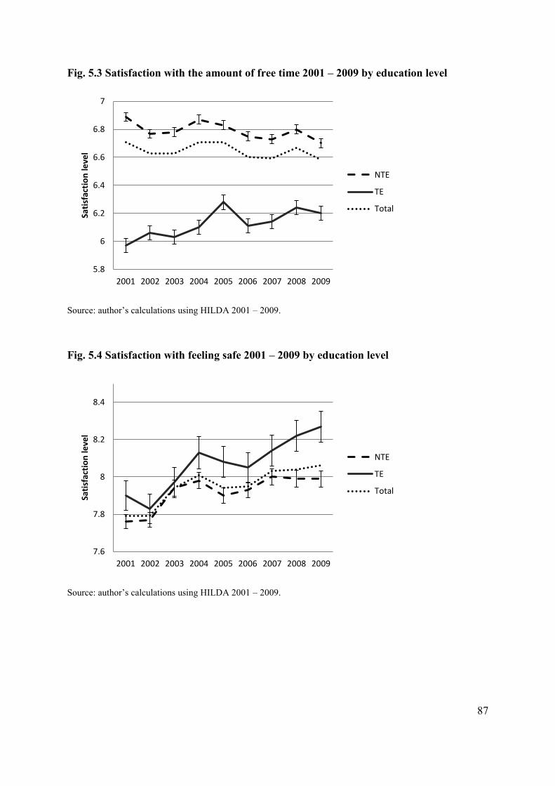
87
Fig. 5.3 Satisfaction with the amount of free time 2001 – 2009 by education level
Source: author’s calculations using HILDA 2001 – 2009.
Fig. 5.4 Satisfaction with feeling safe 2001 – 2009 by education level
Source: author’s calculations using HILDA 2001 – 2009.
5.8
6
6.2
6.4
6.6
6.8
7
2001 2002 2003 2004 2005 2006 2007 2008 2009
Sati
sfac
tio
n le
vel
NTE
TE
Total
7.6
7.8
8
8.2
8.4
2001 2002 2003 2004 2005 2006 2007 2008 2009
Sati
sfac
tio
n le
vel
NTE
TE
Total

88
Fig. 5.5 Satisfaction with own health 2001 – 2009 by education level
Source: author’s calculations using HILDA 2001 – 2009.
Fig. 5.6 Satisfaction with own home 2001 – 2009 by education level
Source: author’s calculations using HILDA 2001 – 2009.
6.6
6.8
7
7.2
7.4
7.6
7.8
2001 2002 2003 2004 2005 2006 2007 2008 2009
Sati
sfac
tio
n le
vel
NTE
TE
Total
7.4
7.6
7.8
8
8.2
2001 2002 2003 2004 2005 2006 2007 2008 2009
Sati
sfac
tio
n le
vel
NTE
TE
Total

89
Fig. 5.7 Satisfaction with own neighbourhood 2001 – 2009 by education level
Source: author’s calculations using HILDA 2001 – 2009.
Fig. 5.8 Satisfaction with feeling part of owns local community 2001 – 2009 by education
level
Source: author’s calculations using HILDA 2001 – 2009.
7.4
7.5
7.6
7.7
7.8
7.9
8
8.1
8.2
2001 2002 2003 2004 2005 2006 2007 2008 2009
Sati
sfac
tio
n le
vel
NTE
TE
Total
6.4
6.5
6.6
6.7
6.8
6.9
7
2001 2002 2003 2004 2005 2006 2007 2008 2009
Sati
sfac
tio
n le
vel
NTE
TE
Total

90
Fig. 5.9 Satisfaction with the partner 2001 – 2009 by education level
Source: author’s calculations using HILDA 2001 – 2009.
7.8
8
8.2
8.4
8.6
8.8
2001 2002 2003 2004 2005 2006 2007 2008 2009
Sati
sfac
tio
n le
vel
NTE
TE
Total

91
Fig. 5.10 Satisfaction with life and satisfaction with domains of life by higher
educational achievement, 2001 – 2009
Source: Author’s calculations using HILDA, 2001-2009.
5.5
6
6.5
7
7.5
8
8.5
2001 2002 2003 2004 2005 2006 2007 2008 2009
Sati
sfac
tio
n le
vel
Overall satisfaction NTE
Overall satisfaction TE
Home NTE
Home TE
Employment NTE
Employment TE
Financial Situation NTE
Financial Situation TE
Safety NTE
Safety TE
Local com NTE
Local com TE
Health NTE
Health TE
N'hood NTE
N'hood TE
Free time NTE
Free time TE

92
In 2009 the tertiary-educated are significantly less satisfied than the non-tertiary-
educated with only one out of nine domains of life: the amount of free time they had. Not
surprisingly, the TE are more satisfied with their employment opportunities, financial
situation and health, domains of life widely discussed in the literature of human capital
development as being influenced by occupational status (Becker, 1964), a proxy for
educational achievement. The tertiary-educated are also more satisfied with their safety
(Table 5.2.d and Fig.5.5) and feeling part of their local communities (Table 5.2.e and Fig.
5.9), these findings confirming the higher levels of belongingness and trust associated with
higher educational achievement (as discussed, for example, by van der Meer, 2010), but
perhaps also the better and safer lifestyle that the tertiary-educated can generally afford.
Throughout the nine waves of data analysed, the tertiary-educated have higher levels
of satisfaction with health than the non-tertiary-educated, and these results find support in the
literature (for example, see Cummins, 2006). The novelty in these findings is that the gap
between the levels of satisfaction of the two groups has increased from some 0.3 points in
2001 to over 0.5 points in 2009 (p<.05, see Table 5.2f). The increase in this gap can be
attributed partially to higher levels of satisfaction for the tertiary-educated and the lower
levels for the non-tertiary-educated compared to 2001 (Table 5.2-f and Fig. 5.6).These
findings flag possible problems in the health system, or in access to health services. The
policy implications of these findings are discussed in Chapter 10, Section 10.2.
The levels of satisfaction with areas of life relating to housing, such as neighbourhood
(Table 5.2-g and Fig. 5.8) or local community (Table 5.2-h and Fig.5.9), have gone through
most variation in the past decade. The tertiary-educated were constantly less satisfied with
their homes (p<.05, Table 5.2-a, and Fig.5.7). Why this is the case is still to be explored. The
reasons behind changes in satisfaction with domains of life are complex most of the time and
may be fully explained only through further in-depth investigation (eg: studies that focus on
satisfaction with housing per se). This is outside the purpose of the thesis. Chapter 7 does,
however, explore how socio-economic and demographic factors impact on satisfactions with
domains of life and the possible policy implications of these findings are discussed in Chapter
10.
Within-group comparisons show that satisfaction with employment opportunities,
financial situation, and safety, increased between 2001 and 2009for both the tertiary-educated
the non-tertiary-educated (p<.05, see Table 5.2.b-d). However, the between-group

93
comparisons reveal that the tertiary-educated are constantly more satisfied with these aspects
of life than the non-tertiary-educated. Although the between-group differences are as small as
0.1 points, they are statistically significant (p<.05).
The analysis in this section has explored how the mean levels of satisfaction with life
and satisfaction with nine domains of life have changed between 2001 and 2009. Different
patterns of change have been identified for the tertiary-educated and for the non-tertiary-
educated. It was concluded that in 2009 the tertiary-educated were significantly less satisfied
with only one out of nine domains of life (satisfaction with the amount free time). They are
more satisfied than the non-tertiary-educated with six domains of life (home, employment
opportunities, financial situation, safety, feeling part of the local community, and health).
Despite such higher levels of satisfaction with domains of life, the tertiary-educated are not
more satisfied with their lives overall48 (Table 5.1 and Fig. 5.1). This is controversial
because, as discussed in studies that support the life-domain approach to well-being
(Campbell, 1981; Campbell et al., 1976), higher satisfaction with domains of life should
generate higher overall satisfaction. Such claims become the basis for a further exploration of
whether the decrease in the SWB of the non-tertiary-educated population, and the increase in
the SWB of the tertiary-educated population identified earlier in this chapter (Fig.5.1 and
Table. 5.1) are, in part, due to the changes in satisfaction with domains of life. The impact of
satisfaction with domains of life on overall satisfaction with life is examined in Chapter 6.
The conclusions of this section have been drawn after the statistical significance of
the between-group and within-group differences between 2001 and 2009 was tested (unpaired
sample t-test, significance levels reported in Table 5.2 a-i). To increase the statistical value of
these findings, the between-group variations are further explored by investigating the
frequency distribution of each population around the mean. The specifications of this analysis
and its advantages are discussed below.
48 Although in 2009 the mean levels of satisfaction with life overall are greater for the tertiary educated than for
the non-tertiary educated, the difference between the two means is not statistically significant (p-value>.05, unpaired sample t-test, 2-sided)

94
b. Distribution of satisfaction with life and satisfaction with domains of life, 2009
An analysis of the distribution of the satisfaction levels within the tertiary-educated and the
non-tertiary populations is conducted in this section (Table B1 in Appendix B and Fig. 12 to
Fig. 20 below). To illustrate the importance of the approach, consider the following example.
Group 1 and Group 2, consisting of five individuals each, have the same mean level
of satisfaction, 5.2, measured on a scale from 0 to 10. Given this, it can be concluded that
there are no differences in the satisfaction between the two groups. Consider, for example,
that within Group 1, the satisfaction of the five individuals is 5, 5, 5, 5, and 6, giving a mean
of 5.2. Within the Group 2, however, the individual levels of satisfaction are 2, 2, 2, 10, and
10, resulting, again, in a mean of 5.2. The difference between the two groups is that the first
one is more homogeneous, with very few inequalities within the population. Within the
second group, however, the individuals are clustered into either very unsatisfied (level 2) or
very satisfied (level 10). The analysis of distributions explores such differences within
populations, bringing further significance to the analysis of means conducted above.
The calculations in this section differentiate between the satisfaction levels of the
tertiary-educated and those of the non-tertiary-educated. One of the most interesting findings
is that more tertiary-educated than non-tertiary-educated individuals consider themselves
somewhat satisfied with life overall (ranking from 6 to 9 on the 0-10 scale), and a higher
proportion of the non-tertiary-educated consider themselves either neither satisfied or
dissatisfied (score of 5 on the 0-10 scale) or totally satisfied (score of 9 and above on the 0-10
scale). This finding is rather revealing in the context of the analysis conducted in the first
section of this chapter. Although the difference of mean scores is not statistically significant,
the distribution of individual scores across the two groups is different, with more tertiary-
educated having higher levels of satisfaction with life. The results suggest an overall larger
proportion of tertiary-educated individuals to have above average levels of overall
satisfaction.49
49 The higher proportion of NTE individuals to report a score or 10 (totally satisfied) is also an interesting
finding; however, it is difficult to explain. It can be discussed from a methodological perspective (more outliers in the NTE sample). Psychologists interested in the study of happiness also discuss the rare cases when individuals find themselves ‘totally satisfied’, including the possibility of errors due to individuals inability to assess own wellbeing, such as in the case of mental illnesses. Veenhoven (1991) discusses the hell-Paradise scenarios, when for example one perceives his bad conditions as good (fake Paradise).

95
Fig. 5.11 Distribution of satisfaction of life overall by education level, 2009
Source: Author’s calculations using HILDA 2009.
The distributions of scores across the two populations follow similar patterns for
satisfaction with home (Fig. 5.13), employment opportunities (Fig. 5. 14), financial situation
(Fig. 5.15), feeling safe (Fig. 5.16), health (Fig. 5.18), and neighbourhood (Fig. 5.19). The
common trend is that more tertiary-educated than non-tertiary-educated individuals rank their
satisfaction above 6, and more non-tertiary-educated than tertiary-educated individuals rank
theirs at or below 5. This finding is important because it reflects that the higher levels of
mean satisfaction of the tertiary-educated are driven by a larger number of these individuals
that are satisfied and very satisfied.
The tertiary-educated have been found to be significantly less satisfied with the
amount of free time they had (Table 5.2-h and Fig. 5.4). However, when the distribution of
satisfaction levels on the 0-10 scale in 2009 is examined (Fig. 20), the percentage of tertiary-
educated individuals to score their satisfaction between 6 and 8 is much higher than the
percentage of the non-tertiary-educated who have these scores. It can be claimed that the
higher mean level of satisfaction with the amount of free time is driven by the non-tertiary-
educated individuals who rank their satisfaction between 8 and 10.
There is also a clear distinction in terms of satisfaction with feeling safe, employment
opportunities, financial satisfaction and health, in that a much larger proportion of tertiary-
educated individuals rank their satisfaction well above 8. This finding is to be noted because
the overall satisfaction with life is around the value 7.8 (see Table 5.1).
0
5
10
15
20
25
30
35
40
Pe
r ce
nt
Satisfaction level
Satisfaction with life overall
TE
NTE

96
Fig. 5.12 Distribution of satisfaction with home by education level, 2009
Source: Author’s calculations using HILDA 2009.
Fig. 5.13Distribution of satisfaction with employment opportunities by education level,
2009
Source: Author’s calculations using HILDA 2009.
0
5
10
15
20
25
30
35
Pe
r ce
nt
Satisfaction level
Satisfaction with the home in which you live
TE
NTE
0
5
10
15
20
25
30
35
Pe
r ce
nt
Satisfaction level
Satisfaction with employment opportunities
TE
NTE
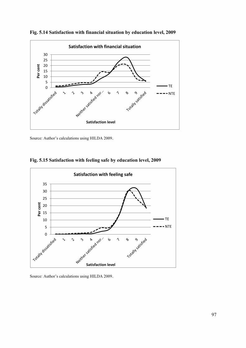
97
Fig. 5.14 Satisfaction with financial situation by education level, 2009
Source: Author’s calculations using HILDA 2009.
Fig. 5.15 Satisfaction with feeling safe by education level, 2009
Source: Author’s calculations using HILDA 2009.
0
5
10
15
20
25
30
Pe
r ce
nt
Satisfaction level
Satisfaction with financial situation
TE
NTE
0
5
10
15
20
25
30
35
Pe
r ce
nt
Satisfaction level
Satisfaction with feeling safe
TE
NTE

98
Fig. 5.16 Satisfaction with feeling part of the local community by education level, 2009
Source: Author’s calculations using HILDA 2009.
Fig. 5.17 Satisfaction with own health by education level, 2009
Source: Author’s calculations using HILDA 2009.
0
5
10
15
20
25
Pe
r ce
nt
Satisfaction level
Satisfaction with feeling part of the local community
TE
NTE
0
5
10
15
20
25
30
35
Pe
r ce
nt
Satisfaction level
Satisfaction with own health
TE
NTE

99
Fig. 5.18 Satisfaction with the neighbourhood by education level, 2009
Source: Author’s calculations using HILDA 2009.
Fig. 5.19 Satisfaction with the amount of free time by education level, 2009
Source: Author’s calculations using HILDA 2009.
-5
0
5
10
15
20
25
30
35
Pe
r ce
nt
Satisfaction level
Satisfaction with the neighbourhood
TE
NTE
0
5
10
15
20
25
Pe
r ce
nt
Satisfaction level
Satisfaction with the ammount of free time
TE
NTE

100
c) Summary of findings
Although across the nine years of data analysed, both the tertiary-educated and the non-
tertiary-educated have experienced increases and decreases in satisfaction with domains of
life, it is more often that the levels of satisfaction of the non-tertiary-educated decreased. In
2009 the tertiary-educated and non-tertiary-educated were found to be equally satisfied with
life overall (overall satisfaction levels of 7.82 and 7.78 respectively, and the difference is not
statistically significant; see Fig.5.1). Nevertheless, when the distribution analysis was
conducted it was concluded that more tertiary-educated individuals rank their overall
satisfaction between 6 and 8, and some non-tertiary-educated (a larger percentage than the
tertiary-educated) rank their satisfaction around the values 5, 9, or 10. This suggests that the
non-difference in satisfaction with life between the two groups is driven by a minority of the
sample.
Furthermore, given the significantly higher satisfaction with six other domains of life
(home, employment opportunities, financial situation, safety, feeling part of the local
community, and health), it can be argued through a life-domain approach that the tertiary-
educated should be more satisfied with their lives overall.50 An aggregate measure of SWB is
calculated to test this, exploring the difference in life-satisfaction between the tertiary-
educated and the non-tertiary-educated in a top-up (or life-domain) approach.
The single item measure (used in the analysis so far) is calculated from the answer to
the general question ‘How satisfied are you with your life overall?’, and the composite
measure is calculated as the average of satisfaction with key domains of life. Whether these
measures of SWB generate similar results is explored in the next section.
5.4 The single-item and multiple-item measures of well-being
5.4.1 Overall satisfaction and average satisfaction, 2009
Studies supporting the life-domain approach claim that life satisfaction is the result of
satisfaction with key domains of life (Cummins, 1996, 2003; Headey and Wearing, 1992;
Rojas, 2004; Veenhoven, 1996; van Praag and Ferrer-i-Carbonell, 2004). Complementary to
the overall satisfaction with life (single-item measure of SWB), an aggregate measure of
SWB is calculated in this chapter as the arithmetic average of the levels of satisfaction with
50 The life-domain approach argues that overall satisfaction is the result of satisfaction with key domains of life,
see literature reviewed in Ch.3, p. 64-66.
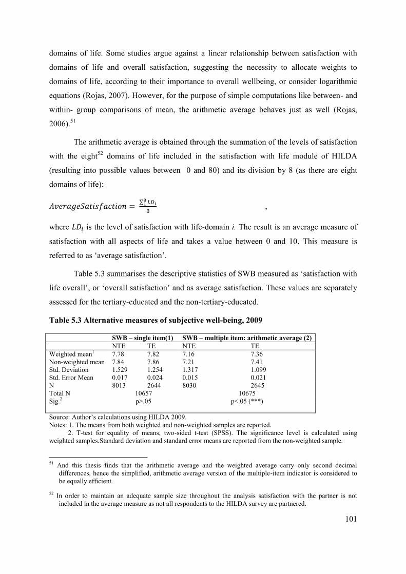
101
domains of life. Some studies argue against a linear relationship between satisfaction with
domains of life and overall satisfaction, suggesting the necessity to allocate weights to
domains of life, according to their importance to overall wellbeing, or consider logarithmic
equations (Rojas, 2007). However, for the purpose of simple computations like between- and
within- group comparisons of mean, the arithmetic average behaves just as well (Rojas,
2006).51
The arithmetic average is obtained through the summation of the levels of satisfaction
with the eight52 domains of life included in the satisfaction with life module of HILDA
(resulting into possible values between 0 and 80) and its division by 8 (as there are eight
domains of life):
∑
,
where is the level of satisfaction with life-domain i. The result is an average measure of
satisfaction with all aspects of life and takes a value between 0 and 10. This measure is
referred to as ‘average satisfaction’.
Table 5.3 summarises the descriptive statistics of SWB measured as ‘satisfaction with
life overall’, or ‘overall satisfaction’ and as average satisfaction. These values are separately
assessed for the tertiary-educated and the non-tertiary-educated.
Table 5.3 Alternative measures of subjective well-being, 2009
SWB – single item(1) SWB – multiple item: arithmetic average (2)
NTE TE NTE TE Weighted mean1 7.78 7.82 7.16 7.36 Non-weighted mean 7.84 7.86 7.21 7.41 Std. Deviation 1.529 1.254 1.317 1.099 Std. Error Mean 0.017 0.024 0.015 0.021 N 8013 2644 8030 2645 Total N 10657 10675 Sig.2 p>.05 p<.05 (***)
Source: Author’s calculations using HILDA 2009. Notes: 1. The means from both weighted and non-weighted samples are reported. 2. T-test for equality of means, two-sided t-test (SPSS). The significance level is calculated using weighted samples.Standard deviation and standard error means are reported from the non-weighted sample.
51 And this thesis finds that the arithmetic average and the weighted average carry only second decimal
differences, hence the simplified, arithmetic average version of the multiple-item indicator is considered to be equally efficient.
52 In order to maintain an adequate sample size throughout the analysis satisfaction with the partner is not included in the average measure as not all respondents to the HILDA survey are partnered.

102
In 2009 the tertiary-educated had –it’s in the past chronologically] higher levels of
overall satisfaction than the non-tertiary-educated but the differences are not statistically
significant (Table 5.3-(1)).This finding was also presented in Section 5.2.1, Table 5.1 where
it was concluded that the tertiary-educated are not significantly more satisfied with their lives
than the non-tertiary-educated, leading towards the confirmation of the paradox of subjective
well-being and tertiary education in Australia. However, when subjective well-being is
calculated as the arithmetic average of satisfaction with domains of life (Table 5.3-2), the
difference between the well-being of the tertiary-educated and the well-being of the non-
tertiary-educated is positive and statistically significant, indicating a positive association
between subjective well-being and tertiary educational achievement. The single-item and
multiple-item measures of SWB lead to diverging conclusions with respect to the paradox of
SWB and tertiary education, suggesting the necessity to further investigate the relationship.
Some additional findings emerge from the comparison above. First, both the TE and
the NTE overestimate their overall satisfaction,53 the tertiary-educated ‘jumping’ in 2009
from an average satisfaction of 7.36 to an overall satisfaction of 7.86, and the non-tertiary-
educated from an average satisfaction of 7.10 to an overall satisfaction of 7.84.
The second finding is that the standard deviation from the mean is higher for both
tertiary-educated and non-tertiary-educated when SWB is measured as overall satisfaction
(single-item measure) than the standard deviation when SWB is measured as average
satisfaction. This suggests that the single-item measure is statistically less reliable
(Wooldridge, 2006).
Finally, it is noteworthy that both standard deviations are greater for the non-tertiary-
educated, pointing towards larger differences between individual levels and mean (and less
consistency across the group, a finding also supported through the analysis of distributions,
Fig. 5.12). The implications of these findings are discussed in Section 10.2, which addresses
the methodological implications of this thesis. The current section concludes that the tertiary-
educated and the non-tertiary-educated have different reports of SWB regardless of the
measurement of assessment used.
The differences in average satisfaction and overall satisfaction between 2001 and
2009 are explored in the next section. The purpose is to investigate whether the relationship
53 Or it can be argued that they underestimate their satisfaction with aspects of life.
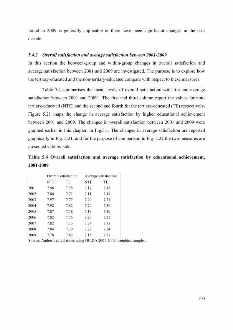
103
found in 2009 is generally applicable or there have been significant changes in the past
decade.
5.4.2 Overall satisfaction and average satisfaction between 2001-2009
In this section the between-group and within-group changes in overall satisfaction and
average satisfaction between 2001 and 2009 are investigated. The purpose is to explore how
the tertiary-educated and the non-tertiary-educated compare with respect to these measures.
Table 5.4 summarises the mean levels of overall satisfaction with life and average
satisfaction between 2001 and 2009. The first and third column report the values for non-
tertiary-educated (NTE) and the second and fourth for the tertiary-educated (TE) respectively.
Figure 5.21 maps the change in average satisfaction by higher educational achievement
between 2001 and 2009. The changes in overall satisfaction between 2001 and 2009 were
graphed earlier in this chapter, in Fig.5.1. The changes in average satisfaction are reported
graphically in Fig. 5.21, and for the purpose of comparison in Fig. 5.22 the two measures are
presented side-by-side.
Table 5.4 Overall satisfaction and average satisfaction by educational achievement,
2001-2009
Overall satisfaction Average satisfaction
NTE TE NTE TE 2001 7.96 7.78 7.17 7.18 2002 7.86 7.71 7.11 7.14 2003 7.97 7.77 7.24 7.24 2004 7.92 7.82 7.24 7.30 2005 7.87 7.78 7.19 7.30 2006 7.82 7.76 7.20 7.27 2007 7.82 7.73 7.24 7.33 2008 7.84 7.79 7.22 7.34 2009 7.78 7.82 7.15 7.37 Source: Author’s calculations using HILDA 2001-2009, weighted samples.

104
Fig. 5.20 Average satisfaction with life by education level, 2001-2009
Source: author’s calculations using HILDA 2001 – 2009. Note: SWB was calculated as the arithmetic average of satisfaction with eight domains of life. Error bars are computed using the 2009 sample size.
Fig. 5.21Overall satisfaction and average satisfaction by education level, 2001 – 2009
Source: author’s calculations using HILDA 2001 – 2009.
6.9
7
7.1
7.2
7.3
7.4
2001 2002 2003 2004 2005 2006 2007 2008 2009
Sati
sfac
tio
n le
vel
NTE
TE
Total
6.6
6.8
7
7.2
7.4
7.6
7.8
8
8.2
2001 2002 2003 2004 2005 2006 2007 2008 2009
Sati
sfac
tio
n le
vel
Overall satisfaction NTE
Overall satisfaction TE
Average satisfaction NTE
Average satisfaction TE

105
The two indicators in Fig. 5.22 are measures of the same concept – subjective well-
being.54 However, the two indicators reveal various between- and within-group differences
when their means are separately plotted for the tertiary-educated and for the non-tertiary-
educated across the nine years of data analysed (2001-2009).
Firstly, overall, between 2001 and 2009 there is a considerable gap of approximately
0.5 points between the overall satisfaction and average satisfaction of both tertiary-educated
and non-tertiary-educated individuals. Although marginally this difference may be considered
relatively small, in the context of subjective well-being studies, such a gap is considered
generous55. Secondly, between 2001 and 2009 the average satisfaction of the non-tertiary-
educated (single dotted line) has hardly changed (remaining approximately at 7.2), while that
of the tertiary-educated has increased marginally. On the other hand, the overall satisfaction
has hardly changed for the tertiary-educated (double continuous line) and has decreased for
the non-tertiary-educated, a finding also pointed to in Section 5.2.1. Finally, at the between-
group level, the overall satisfaction of the tertiary-educated and the non-tertiary-educated has
converged towards the same value while the difference in average satisfaction of the two
groups has widened; by 2009 the tertiary-educated having higher levels of average
satisfaction than the non-tertiary-educated.
5.5 Conclusion
The aim of this chapter has been to investigate whether the tertiary-educated are less satisfied
with life and with domains of life than the non-tertiary-educated. The analysis of the last
available wave of data from the HILDA (2009) survey indicates that tertiary-educated
Australians are more satisfied with 6 out of 9 domains of life, partially supporting Hypothesis
1-a of the thesis. Hypothesis 1-b, however, was more difficult to assess.
In Section 5.3 the difference between the levels of overall satisfaction with life of the
tertiary-educated and of the non-tertiary-educated was identified as positive but statistically
non-significant (Table 5.1). This was a primary reason to reject Hypothesis 1-b, which claims
that there is no paradox of SWB and higher education in Australia. 54Fig. 5.22 can be understood as the graphic representation of SWB as defined in the top-down and bottom-up
approaches respectively. The bottom-up approach assumes that high overall satisfaction is the results of high satisfaction with domains of life (average satisfaction in Fig. 5.22), while the top-down approach assumes that satisfaction with life, measured as a single-item (overall satisfaction in Fig. 5.22) drives high satisfaction with various aspects of life.
55SWB is a measure that rarely fluctuates (Cummins, 2000) and when they happen, fluctuations are minimal.

106
However, in Section 5.4 an alternative measure of SWB was calculated as the
arithmetic average of the levels of satisfaction with domains of life. Results from this analysis
were most surprising. Firstly, this average satisfaction was calculated around the value of 7.2
(on a 0 to 10 scale), compared to an overall satisfaction at the value of approximately 7.8 (see
Table 5.4 and Fig. 5.22). Given that the two indicators are measures of the same concept, this
finding is noteworthy. Secondly, the findings summarised in Table 5.4 and Fig .5.22 above
revealed that although in the past decade the tertiary-educated and the non-tertiary-educated
have merged towards the same levels of overall satisfaction, the difference between their
levels of average satisfaction widened out. Accordingly, the tertiary-educated have had
significantly higher levels of average satisfaction (arithmetic average of satisfaction with
domains of life) than the non-tertiary-educated since 2004, allowing for Hypothesis 1-b to be
confirmed.
Therefore, the paradox has been both refuted and confirmed in this chapter. The
conclusion is that the relationship between subjective well-being and tertiary educational
achievement is dependent on the measure of subjective well-being employed. The thesis
maintains through its theoretical approach that subjective well-being is sensitive to
perceptions of well-being, and based on this it is maintained that average satisfaction is the
‘appropriate’ measure of SWB. However, to be able to conclude that there is no paradox of
SWB and tertiary education it is also necessary to support the theoretical claims through
empirical analysis. For this reason the next chapter explores how the tertiary-educated and the
non-tertiary-educated conceptualise SWB, or ‘what counts’ towards their well-being.

107
Chapter 6 Findings: The heterogeneity of SWB by
education
6.1 Introduction
In this chapter, the heterogeneity of subjective well-being by higher educational achievement
is empirically explored. Its theoretical grounds have been discussed in Chapter 2. This
empirical exploration has reached the conclusion that the negative relationship between SWB
and higher education previously identified in the literature is the result of measurement
biases56
SWB is an inherently inferential and subjective measure of well-being (Rojas, 2006),
prone to individual biases such as personality (Diener and Lucas, 1999), and the tendency to
compare one’s achievements with one’s own and others’ expectations, and with previous
experiences (Michalos, 1985). Like studies such as those of Cummins (1998, 2003), Headey
and Wearing (1992), Veenhoven (1996) and Rojas (2007), this chapter interprets life
satisfaction as a general construct of satisfaction with key aspects of life.
The purpose of this chapter is to assess the heterogeneity of SWB by tertiary-
educational achievement using national representative data from the HILDA 2001 and
HILDA 2009 surveys, and test the second hypothesis (2-a) of the thesis:
2) a) SWB is heterogeneous by higher educational achievement.
The correlations between SWB and satisfaction with eight domains of life57 (ranked
from 0 to 10 with 0 least satisfied and 10 most satisfied) are explored in the second section of
the chapter. This analysis sheds light on the ‘bundle’ of aspects of life that count towards the
SWB of the tertiary-educated and non-tertiary-educated, and on whether the two sub-
populations are different in this respect. The third section of the chapter is an in-depth
investigation of the impact on overall satisfaction, of satisfaction with these domains of life.
56 As explained in Chapter 1, Section 1.3, a bias is defined in the thesis as occurring when a response to a test
item tends to be altered in such a way that it indicates something other than what it is intended to measure Runquist (1950)..
57 The same eight domains explored in Chapter 5 are further explored in this chapter. Satisfaction with partner is not considered because not all respondents to the HILDA survey were partnered, and this has reduced the sample size.

108
6.2 Correlations between domains of life and satisfaction with life, 2001 and 2009
Changes in the levels of SWB between 2001 and 2009 were explored in Chapter 5 (Fig.
5.12), and it was concluded that the tertiary-educated and the non-tertiary-educated have
converged in their overall satisfaction, but that the difference between the two groups in
average satisfaction with domains of life has widened.
Studies exploring the relationship between single-item measures and multiple-item
measures of SWB conclude that, while there are conceptual differences between the two
means of measurement, ‘if the focus of one’s research is to get a relatively reliable and valid
measure of well-being and one cannot afford to include a variety of self-report indicators, one
can confidently assess these constructs using single-item measures’ (Diener, 2009: 88). This
thesis has found, however, that the conceptual differences matter.
The correlation between the single-item (overall satisfaction) and multiple-item
(average satisfaction) measures of SWB is tested for 2001 and 2009, both for the entire
sample and separately for the tertiary-educated and the non-tertiary-educated. Pearson
correlation tests have been conducted in SPSS and Table 6.1 summarises the results.
Table 6.1 Correlation levels between single-item and multiple-item measures of SWB, 2001 and 2009 by higher educational achievement
2001 2009 All .620** .666** NTE .616** .657** TE .660** .709**
Source: Author’s calculations using HILDA, 2001 and HILDA 2009. Note: Pearson Correlation, sig is 2-tailed. **correlation is significant at 0.01 level.
The two measures of SWB correlate more strongly in 2009 than in 2001, and the
absolute increase in the level of correlation is similar for the NTE58 and the TE. However,
these correlations are higher for the TE. This is the first indication that the concepts of overall
satisfaction and average satisfaction are not the same for the TE and the NTE.
The extent to which satisfaction with domains of life correlates with overall
satisfaction is further explored. This correlation analysis is conducted for 2001 and 2009, and
Table 6.2 summarises the findings for 2001. The top-right quadrant of the table reports the
correlations between satisfaction with domains of life and satisfaction with life in general for
58 As mentioned in the list of acronyms, although the author prefers to spell out these terms, the acronyms are
used at a time when the results from the analysis are reported.
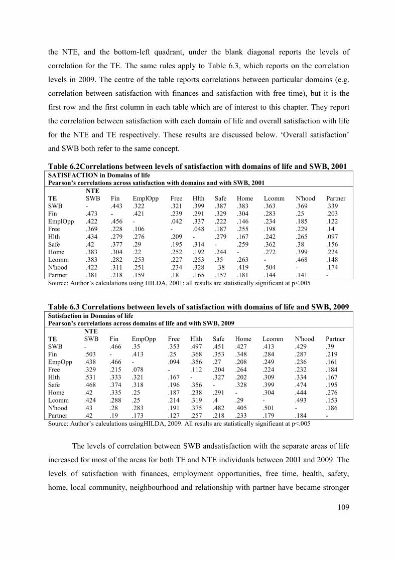
109
the NTE, and the bottom-left quadrant, under the blank diagonal reports the levels of
correlation for the TE. The same rules apply to Table 6.3, which reports on the correlation
levels in 2009. The centre of the table reports correlations between particular domains (e.g.
correlation between satisfaction with finances and satisfaction with free time), but it is the
first row and the first column in each table which are of interest to this chapter. They report
the correlation between satisfaction with each domain of life and overall satisfaction with life
for the NTE and TE respectively. These results are discussed below. ‘Overall satisfaction’
and SWB both refer to the same concept.
Table 6.2Correlations between levels of satisfaction with domains of life and SWB, 2001 SATISFACTION in Domains of life Pearson’s correlations across satisfaction with domains and with SWB, 2001 NTE TE SWB Fin EmplOpp Free Hlth Safe Home Lcomm N'hood Partner SWB - .443 .322 .321 .399 .387 .383 .363 .369 .339 Fin .473 - .421 .239 .291 .329 .304 .283 .25 .203 EmplOpp .422 .456 - .042 .337 .222 .146 .234 .185 .122 Free .369 .228 .106 - .048 .187 .255 .198 .229 .14 Hlth .434 .279 .276 .209 - .279 .167 .242 .265 .097 Safe .42 .377 .29 .195 .314 - .259 .362 .38 .156 Home .383 .304 .22 .252 .192 .244 - .272 .399 .224 Lcomm .383 .282 .253 .227 .253 .35 .263 - .468 .148 N'hood .422 .311 .251 .234 .328 .38 .419 .504 - .174 Partner .381 .218 .159 .18 .165 .157 .181 .144 .141 - Source: Author’s calculations using HILDA, 2001; all results are statistically significant at p<.005 Table 6.3 Correlations between levels of satisfaction with domains of life and SWB, 2009 Satisfaction in Domains of life Pearson’s correlations across domains of life and with SWB, 2009 NTE TE SWB Fin EmpOpp Free Hlth Safe Home Lcomm N'hood Partner SWB - .466 .35 .353 .497 .451 .427 .413 .429 .39 Fin .503 - .413 .25 .368 .353 .348 .284 .287 .219 EmpOpp .438 .466 - .094 .356 .27 .208 .249 .236 .161 Free .329 .215 .078 - .112 .204 .264 .224 .232 .184 Hlth .531 .333 .321 .167 - .327 .202 .309 .334 .167 Safe .468 .374 .318 .196 .356 - .328 .399 .474 .195 Home .42 .335 .25 .187 .238 .291 - .304 .444 .276 Lcomm .424 .288 .25 .214 .319 .4 .29 - .493 .153 N'hood .43 .28 .283 .191 .375 .482 .405 .501 - .186 Partner .42 .19 .173 .127 .257 .218 .233 .179 .184 - Source: Author’s calculations usingHILDA, 2009. All results are statistically significant at p<.005
The levels of correlation between SWB andsatisfaction with the separate areas of life
increased for most of the areas for both TE and NTE individuals between 2001 and 2009. The
levels of satisfaction with finances, employment opportunities, free time, health, safety,
home, local community, neighbourhood and relationship with partner have became stronger

110
predictors of SWB for both groups. However in 2009, satisfaction with some domains of life
(financial situation, employment opportunities, health and partner) correlated more strongly
with SWB for the TE than for the NTE.
It can be concluded that the levels of satisfaction with particular aspects of life relate
to the levels of overall satisfaction (SWB) to a different extent for the tertiary-educated and
the non-tertiary-educated. This is the first piece evidence supporting the hypothesis that SWB
is heterogeneous by higher educational achievement. However, further regression analysis is
necessary to assess the actual effect that the change in satisfaction with each of these domains
has over the SWB of the two groups. This regression analysis is conducted in the next
section.
6.3 Impact of satisfaction with domains of life on SWB, 2001 and 2009
6.3.1 Well-being in 2009
The impact on SWB of satisfaction with domains of life is explored using semi-logarithmic
specifications59 in an Ordinary Least Squares (OLS) regression of satisfaction with domains
of life on overall satisfaction (SWB). The model used is:
∑ ( ) (6.1)
The same domains of life as above are used in the analysis. However, the 0 to 10 scores are
multiplied by 10 and expressed in logarithmic form. In the model above, LDi are the
respective life domains, are the parameters to be estimated and µ is the error term to
include factors unobserved and uncontrolled for. Results are summarised in Table 6.4. A
reduced model was run first, using only the eight aspects of life included in the ‘satisfaction
with life’ module in HILDA (Model 1 in Table 6.4). By controlling for satisfaction with the
partner, a second model was regressed to explore how satisfaction with personal life relates to
overall SWB (Model 2 in Table 6.4). Separate regressions for the TE (Bachelor, Pasters and
PhD) and the NTE (other post-secondary, secondary and less than secondary) are conducted,
in order to explore the heterogeneity of SWB by higher educational achievement. To remind
the reader, a regression for the entire population with controls for higher-educational level
achieved was not conducted because this was the very purpose of the analysis, that is, to 59 Rojas (2004) notes the importance of using semi-logarithm specification in assessing the impact on SWB of
domains of life, because the more widely used linear specifications require strong and unrealistic assumptions (Rojas, 2004). The argument is that the impact on SWB of greater satisfaction in particular domains of life is contingent on individual initial levels of satisfaction, and as life-domain satisfaction increases the additional impact on SWB reduces (diminishing returns).

111
prove that there are conceptual differences in how the TE and the NTE assess their SWB.
SWB cannot be the dependent variable in a regression model that includes both TE and NTE
respondents.
Adjusted R-square values of over 0.450 indicate an appropriate goodness-of-fit for
both models in Table 6.4. Results are discussed below. Because the model used is semi-
logarithmic (independent variables have been log-transformed), the results are rather
straightforward. If satisfaction with a domain of life increases by 100 per cent, the overall
satisfaction (SWB) increases by the beta coefficient. Although such changes seem very small,
they are relevant when assessed in the context of subjective well-being studies, where
variations are generally small.
The results in Table 6.4 reveal that satisfaction levels with some domains of life have
a greater impact on the SWB of tertiary-educated individuals than on that of the non-tertiary-
educated.
For example, in Model-1 (when satisfaction with the partner is not included),
satisfaction with finances, employment opportunities, and local community and
neighbourhood, impact on the SWB of the TE more than on that of the NTE. On the other
hand, levels of satisfaction with free time and home have a greater impact on the overall
satisfaction of the NTE than on the that of the TE. These findings indicate that satisfaction
with domains of life contribute to the SWB of the TE and the NTE to a different extent. In
other words, the results from the semi-logarithmic model (6.1) support the heterogeneity of
SWB by higher-educational achievement, confirming Hypothesis 2-a. A few other findings
that point towards the differences between the tertiary-educated and non-tertiary-educated are
discussed below.
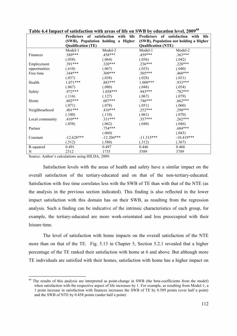
112
Table 6.4 Impact of satisfaction with areas of life on SWB by education level, 200960 Predictors of satisfaction with life
(SWB), Population holding a Higher Qualification (TE)
Predictors of satisfaction with life (SWB), Population not holding a Higher Qualification (NTE)
Model-1 Model-2 Model-1 Model-2 Finances .589***
(.058) .458*** (.064)
.459*** (.036)
.363*** (.042)
Employment opportunities
.391*** (.610)
.320*** (.067)
.236*** (.035)
.228*** (.040)
Free time .344*** (.037)
.309*** (.038)
.505*** (.028)
.460*** (.031)
Health 1.071*** (.067)
.883*** (.080)
1.008*** (.048)
.933*** (.054)
Safety .972*** (.116)
1.058*** (.127)
.943*** (.067)
.782*** (.079)
Home .602*** (.071)
.607*** (.078)
.746*** (.051)
.662*** (.060)
Neighbourhood .401*** (.100)
.410*** (.110)
.252*** (.061)
.290*** (.070)
Local community .410*** (.058)
.331*** (.062)
.357*** (.040)
.262*** (.046)
Partner .754*** (.060)
.684*** (.043)
Constant -12.628*** (.512)
-12.204*** (.580)
-11.315*** (.312)
-10.419*** (.367)
R-squared 0.491 0.497 0.446 0.466 N 2312 1735 5589 3789 Source: Author’s calculations using HILDA, 2009.
Satisfaction levels with the areas of health and safety have a similar impact on the
overall satisfaction of the tertiary-educated and on that of the non-tertiary-educated.
Satisfaction with free time correlates less with the SWB of TE than with that of the NTE (as
the analysis in the previous section indicated). This finding is also reflected in the lower
impact satisfaction with this domain has on their SWB, as resulting from the regression
analysis. Such a finding can be indicative of the intrinsic characteristics of each group, for
example, the tertiary-educated are more work-orientated and less preoccupied with their
leisure time.
The level of satisfaction with home impacts on the overall satisfaction of the NTE
more than on that of the TE. Fig. 5.13 in Chapter 5, Section 5.2.1 revealed that a higher
percentage of the TE ranked their satisfaction with home at 6 and above. But although more
TE individuals are satisfied with their homes, satisfaction with home has a higher impact on
60 The results of this analysis are interpreted as point-change in SWB (the beta-coefficients from the model)
when satisfaction with the respective aspect of life increases by 1. For example, as resulting from Model-1, a 1 point increase in satisfaction with finances increases the SWB of TE by 0.589 points (over half a point) and the SWB of NTE by 0.458 points (under half a point)

113
SWB for the NTE. The implications of these findings are later discussed in the context of
policy in Chapter 10.
Satisfaction with the partner has a slightly higher impact on the SWB of the TE than
on that of the NTE. The introduction of this last factor into the analysis also slightly reduces
the impact of the other domains of life on SWB. For example, financial satisfaction has a
lower impact on SWB when satisfaction with the partner is considered, regardless of the level
of education. Similarly, the impact on SWB of satisfaction with domains like employment
opportunities, free time, health and local community, reduces for both the TE and NTE when
satisfaction with the partner is controlled for. This reduction in coefficient, however, may
also only be the effect of having introduced another control variable into the equation,
reducing the elements in the error terms and increasing the number of factors that explain the
variation in the dependent variable (Wooldridge, 2006).
Nevertheless, these results converge towards one main finding: satisfaction with
domains of life does not have the same impact on the SWB of the TE and NTE. The
heterogeneity of SWB by educational achievement is thus reinforced by these results,
confirming hypothesis 2-a.The analysis in Chapter 5 identified various changes in the levels
of SWB and satisfaction with domains of life, and more importantly, that these changes are
different for the TE and the NTE. For this reason, the impact on SWB of satisfaction with
domains of life is also explored using 2001 data.
6.3.2 Well-being in 2001, and comparison with 2009
The aim of this subsection is to explore the question of whether the contribution of
satisfaction with various domains of life to the overall satisfaction of the tertiary-educated
and the non-tertiary-educated has changed over time, and to explain the between- and within-
group variations in SWB identified in Chapter 5.
The author acknowledges that the conventional model for exploring the impact of an
independent variable on the same dependent variable across two periods of time is pooled-
OLS (for a non-repeated sample), using year dummies and interaction terms (Wooldridge,
2006). However, this model cannot be applied because perceptions of well-being are likely to
change across time (life-course theory). In other words, the dependent variable, although
measured on the same 0 to 10 scale, is not the same conceptually across the two periods.
Similarly, statistical significance was not calculated for the difference in coefficients for TE

114
and NTE, because doing so assumes that the same dependent variable SWB can be included
in the multivariate equation for both the TE and NTE. But this is not the case – it is this very
heterogeneity of SWB by higher-educational achievement that this analysis seeks to explore.
The same semi-logarithmic model as above (Section 6.1) is tested in this subsection
using 2001 HILDA data. The results from the 2001 and 2009 analyses are then compared.
Table 6.5 summarises these findings.61The left-hand side of the table reports on the factors
that impacted on the SWB of the tertiary-educated in 2001 and 2009. The two columns on the
right-hand side of the table report on the impact of satisfaction with domains of life on the
SWB of the non-tertiary-educated in 2001 and 2009. Results are briefly discussed below, and
their wider policy, theoretical and methodological implications are presented in Chapter 10.
Table 6.5 Semi-logarithmic analysis of the impact of satisfaction with domains of life on overall satisfaction 2001 and 2009 Predictors of satisfaction with life
(SWB), Population holding a Higher Qualification (TE)
Predictors of satisfaction with life (SWB), Population not holding a Higher Qualification (NTE)
2001 2009 2001 2009 Finances 0.585***
(.061) .589*** (.058)
0.516*** (.032)
.459*** (.036)
Employment opportunities
0.422*** (.060)
.391*** (.610)
0.307*** (.032)
.236*** (.035)
Free time 0.358*** (.042)
.344*** (.037)
0.419*** (.026)
.505*** (.028)
Health 1.002*** (.080)
1.071*** (.067)
0.882*** (.046)
1.008*** (.048)
Safety 0.447*** (.093)
.972*** (.116)
0.702*** (.050)
.943*** (.067)
Home 0.562*** (.072)
.602*** (.071)
0.677*** (.045)
.746*** (.051)
Neighbourhood 0.369*** (.099)
.401*** (.100)
0.398*** (.051)
.252*** (.061)
Local community 0.430*** (.065)
.410*** (.058)
0.330*** (.036)
.357*** (.040)
Constant -19.454*** (.755)
-12.628*** (.512)
-19.657*** (.431)
-11.315*** (.312)
R-squared 0.434 0.491 0.376 0.446 N 2129 2312 7860 5589 Source: Author’s calculations using HILDA, 2001 and HILDA, 2009.
The impact of satisfaction with each domain of life on the SWB of the tertiary-
educated and the non-tertiary-educated is discussed in order of their inclusion in the analysis
and in Table 6.5. Satisfaction with finances became a weaker predictor of SWB for the NTE 61The extended model, which included satisfaction with the partner,was also run, but because the results were
rather similar to those from the reduced model drawing on a larger population, the latter was chosen for presentation in this chapter.

115
in 2009 compared to 2001, while the impact of this domain of life on the SWB of the TE
marginally increased in the same period of time.
Being satisfied with the amount of free time correlates better with the SWB of the
NTE than with the SWB of the TE. Fig.5.4 in Chapter 5, Section 5.2.1 also showed that the
non-tertiary-educated were more satisfied with their free time than the tertiary-educated, both
in 2001 and 2009. These findings are important for the life-balance discourse. However, in
the context of this analysis, the notable fact is that the two sub-populations are different in
this respect.
Satisfaction with health is the area with by far the greatest impact on SWB, for both
tertiary-educated and non-tertiary-educated individuals. Furthermore, the impact of this
variable on SWB increased between 2001 and 2009 for both the TE and the NTE. However,
the TE are more satisfied with their health than the NTE, and the gap between the two groups
widened between 2001 and 2009 (see Fig. 5.6 in Chapter 5, Section 5.2.1). Despite the
importance all individuals give to satisfaction with health, the needs of the NTE seem to be
unmet. The policy implications of these findings are discussed in Chapter 10.
The largest change, for all individuals, occurred in the impact of safety on overall
satisfaction with life. In 2001 satisfaction with safety had less of an impact on the SWB of the
TE than on the SWB of the NTE. However, by 2009, the impact of satisfaction with safety on
the SWB of the TE had increased dramatically. It nearly doubled, to a level higher than the
impact of satisfaction with this aspect of life on the SWB of the NTE. Nevertheless, the
impact of satisfaction with safety increased for the non-tertiary-educated as well, by about 20
per cent. Although this is a great change for both groups, it is difficult to know what might
have caused this increase. It could be, for example, the international awareness of safety
issues following the 9/11 terrorist attack on the U.S., or it could be something in Australia
making people more aware of the importance of safety. Such explanations, however, can only
remain at the stage of speculation until further in-depth analysis.
The impact on overall satisfaction of satisfaction with home has increased for the TE,
and so has the impact of satisfaction with their neighbourhood. While the same trend is
evident for the NTE in the case of satisfaction with home, satisfaction with neighbourhood
has had less of an impact for this group. The NTE were more satisfied with home than the TE
between 2001 and 2009, indicating a low level of satisfaction with housing on the part of the
tertiary-educated. This in turn seems to be affecting their overall satisfaction with life at quite
116
a high rate. Whether these differences are due to poor housing conditions, or the scarcity of
homes, or is just due to adaptation and comparison with peers, is yet to be explored. It is
interesting, however, that housing is an area that the tertiary-educated are not satisfied with,
and an increase in satisfaction with their homes could well increase their overall well-being.
6.4 Conclusion
Some studies explore subjective well-being through a life-domain approach and argue that
individuals have different levels of SWB depending on demographics like gender, age or
income (Clark et al., 2005, Rojas, 2006, Plagnol, 2010). This thesis claims that subjective
well-being is heterogeneous (or clustered) by higher educational achievement, that is, the
tertiary-educated and the non-tertiary-educated have different perceptions of ‘what counts’
towards well-being.
This chapter tested the heterogeneity of SWB by higher-educational achievement
using a life-domain approach,. Findings from correlation and regression analyses confirm the
second hypothesis (2-a) of the thesis, that satisfaction with particular aspects of life
contributes to the SWB of the tertiary-educated and the non-tertiary-educated to a different
extent. This finding indicates that, when asked the general question ‘How satisfied are you
with your life these days?’ the tertiary-educated and the non-tertiary-educated give different
weights to the different aspects of their lives. The conclusion following from this finding is
that this common indicator of SWB includes measurement errors, even though it is measured
on the same 0 to 10 scale for both TE and NTE individuals. For example, the tertiary-
educated give more weight to satisfaction with job opportunities, finances and safety when
assessing their ‘satisfaction with life overall, all things considered’, while the non-tertiary-
educated give more weight to satisfaction with their homes and free time.
The central finding in this chapter is that ‘overall satisfaction’, the single-item
measure of SWB, incorporates conceptual differences. The conclusion is that the aggregate
measure of well-being, as the average of the levels of satisfaction with domains of life,is a
more accurate measure of well-being and is generally preferred. When SWB is assessed
through this aggregate measure (Chapter 5, Fig.5.11), the paradox of SWB and tertiary
education disappears.
Nevertheless, despite the possible conceptual errors it incorporates, the single-item
measure of SWB is often used in national and international surveys and studies that inquire
117
about subjective well-being (e.g. World Values Survey, GSOEP). Findings from this chapter
and from Chapter 5 lead to the conclusion that the relationship between SWB and tertiary
education is not negative. The theoretical framework for the heterogeneity of SWB by higher-
educational achievement was developed in Chapter 2, and this chapter brought the empirical
support. Chapter 7 further explores why the differences in the reported well-being occur
when the single-item and multiple-item measures of SWB are employed.

118
Chapter 7 Findings: The impact of socio-economic and
demographic factors on well-being
7.1 Introduction
This chapter explores how socio-economic and demographic factors affect the SWB of the
tertiary-educated and non-tertiary-educated. Relevant demographic factors like gender,
marital status, geographic location, socio-economic status and cultural background are
considered. Hypothesis 2-b of the thesis is tested in this chapter:
H 2-b) The factors that impact SWB are different for the tertiary-educated and non-
tertiary-educated.
The aim of the chapter is to establish whether external factors have the same impact on the
SWB of the tertiary-educated as on that of the non-tertiary-educated. The impact of these
demographics on satisfaction with the eight domains of life is also explored. It is not
appropriate to measure the impact of external factors on well-being averaged across the eight
domains, because some demographics may impact differently on different domains of life,
and an ‘aggregate effect’ obtained by regressing demographic variables on average
satisfaction would neglects such individual interactions. For this reason SWB is measured as
overall satisfaction.
The data, the regression model and the variables included in the analysis are described
in Section 7.2. Section 7.3 presents the results of the analysis conducted using data from the
HILDA 2009. How each explanatory factor impacts on overall satisfaction and on
satisfaction with each of the domains of life is discussed, and the differences between the
tertiary-educated and non-tertiary-educated are explained. In Section 7.4 the same analysis is
conducted using HILDA 2001 data, and the results are compared to those obtained in Section
7.3. This comparison is important in the context of policy because it explores whether some
factors have become stronger predictors of subjective well-being in the past decade.
7.2 The model and data description
Cross-sectional analysis of 2009 data is conducted, using the refreshed sample of 13,301
respondents, excluding those younger than 25 (remaining n=10,675 individuals). Population
weights are used for means and standard errors, although the un-weighted samples are used

119
for regression analysis. An ordered logit regression in robust standard errors explores the
factors that impact SWB and satisfaction with domains of life:
∑ (7.1)62,
where Y is the dependent variable, the self-assessed satisfaction with domain of life j for
individual i, α is the intercept (or constant) for each domain of satisfaction (j), βk are the
coefficients that indicate the size of the impact factors xk have for individual i over life
domain j; xk are independent variables included in the equation to control for demographics
like gender, age, geographic area, marital status and whether the person has children, health
or income. These variables are described in Table 7.1.
Table 7.1Description of variables used in the ordered logit model of satisfaction with life and domains of life Variable Description Life satisfaction Self-declared satisfaction with life overall and with eight domains of life, with 0 most
dissatisfied and 10 most satisfied Female Gender variable, takes value 1 if respondent is female ATSI Aboriginal or Torres Strait Islander (ATSI) background variable, takes value 1 if
respondent is of ATSI background CALD Identifies individuals culturally and linguistically diverse (CALD), takes value 1 if
respondent is of CALD background Other Urban Geographic location variable, takes value 1 if respondent lives in a metropolitan area
other than major metropolitan Rural Geographic location variable, takes value 1 if respondent lives in a bounded locality and
rural balance Unemployed Employment variable, takes value 1 if respondent is unemployed NILF Employment variable, takes value 1 if respondent is not in the labour force Higher Education Education variable, central to the thesis, takes value 1 if respondent completed a tertiary
qualification (Bachelor, Graduate Diploma, Masters, PhD) Single Marital status variable, takes value 1 if respondent is single Separated Marital status variable, takes value 1 if respondent is separated Divorced Marital status variable, takes value 1 if respondent is divorced Widowed Marital status variable, takes value 1 if respondent is widowed w/Children Variable takes value 1 if respondent has children Income: 1st quartile Income variable, takes value 1 if respondent is in the first income quartile Income: 2nd quartile Income variable, takes value 1 if respondent is in the second income quartile Income: 4th quartile Income variable, takes value 1 if respondent is in the fourth income quartile In bad health Health variable, takes value 1 if respondent has a long term disease or disability Source: HILDA, 2009.
The reference person in the regression model is male, age 35-44 years, living in a
major metropolitan area, employed, married, without children, without tertiary education, in
62This model was preferred for ease of comparison of results, as the independent variables are dummy variables
taking the values 0 or 1. Under the specifications of this model, the response variable level is expected to change by its respective regression coefficient in the ordered log-odds scale.
120
good health, non-ATSI, non-CALD, in the third income quartile63. This regression wasfirst
conducted for the entire sample, flagging individuals with tertiary qualifications through the
inclusion of a dummy variable that equals 1 if the person had completed tertiary studies by
2009. Consistent with findings in the literature (Headey and Wooden, 2004; Dockery, 2010),
the impact of tertiary education on SWB was not statistically significant. These results are not
reported because the approach is outside the purpose of the thesis investigating the
heterogeneity of SWB by educational achievement (i.e. a common measure of SWB should
not be used for both the tertiary-educated and the non-tertiary-educated, because what counts
for SWB is different for the two groups). Hence the model described above (Section 7.1), for
exploring factors that impact on life-satisfaction and satisfaction with domains of life of each
group, is separately tested for the tertiary-educated and the non-tertiary-educated. Results are
reported and discussed in the next section. The interpretation of the results from the ordered
logit model is that for a one unit increase in the predictor, the response variable level is
expected to change by its respective regression coefficient in the ordered log-odds scale. See
Wooldridge, 2007 for the complete specifications of the ordered logit model.
7.3 Findings, 2009
The impact of each demographic variable on overall satisfaction and satisfaction with each
domain of life is discussed in order of their inclusion in the regression: gender, ethnicity,
Aboriginal status, health status, employment status, geographic location, marital status, age,
and income. The findings are summarised in Tables7.2.a and 7.2.b.
63 Household equivalised income is used in the main analysis and income quartiles were derived. Later in the
chapter differences between this measure and the use of personal income are discussed. Household equivalised income is calculated as total household income divided by the square root of the total number of household members.

121
Table 7.2.aFactors impacting SWB and satisfaction with domains of life SWB Free time Health Safety Home TE NTE TE NTE TE NTE TE NTE TE NTE female 0.18* 0.12* -0.13 -0.18*** 0.03 0.14** -0.18* -0.02 0.15 0.03 (0.09) (0.05) (0.08) (0.05) (0.09) (0.05) (0.09) (0.05) (0.08) (0.05) CALD -0.04 -0.12 0.07 -0.18 0.03 -0.11 -0.14 -0.04 -0.36 0.32 (0.28) (0.16) (0.27) (0.16) (0.27) (0.16) (0.28) (0.16) (0.27) (0.16) ATSI 0.01 0.39** 0.48 0.18 -0.64 -0.00 0.24 0.49*** 0.18 0.09 (0.42) (0.14) (0.40) (0.14) (0.37) (0.14) (0.38) (0.14) (0.38) (0.14) Ill health -0.72*** -0.65*** -0.13 -0.01 -1.70*** -1.65*** -0.47*** -0.28*** -0.39** -0.07 (0.13) (0.06) (0.12) (0.06) (0.13) (0.06) (0.12) (0.06) (0.12) (0.06) Unemployed -0.32 -0.42** 1.45*** 1.03*** -0.11 -0.33* 0.07 -0.07 0.60 -0.54*** (0.35) (0.16) (0.31) (0.16) (0.33) (0.15) (0.33) (0.16) (0.33) (0.16) NILF 0.09 0.04 0.73*** 0.72*** -0.24 -0.39*** 0.09 -0.02 0.12 0.08 (0.15) (0.07) (0.15) (0.07) (0.15) (0.07) (0.14) (0.07) (0.15) (0.07) OtherUrban 0.07 0.14* 0.23* 0.16** 0.12 0.02 0.36** 0.15** 0.10 0.18*** (0.11) (0.05) (0.11) (0.05) (0.11) (0.05) (0.11) (0.05) (0.11) (0.05) Rural 0.34** 0.18** 0.18 0.07 0.14 0.11 0.54*** 0.49*** 0.40** 0.31*** (0.13) (0.06) (0.13) (0.06) (0.13) (0.06) (0.13) (0.06) (0.13) (0.06) Single -1.18*** -0.59*** 0.48*** 0.25*** -0.39** -0.11 -0.33** -0.28*** -0.10 -0.11 (0.13) (0.07) (0.12) (0.07) (0.12) (0.07) (0.13) (0.07) (0.13) (0.07) Separated -1.16*** -0.83*** -0.18 -0.03 -0.37 -0.20 -0.29 -0.35** -0.69** -0.41*** (0.23) (0.12) (0.21) (0.12) (0.23) (0.12) (0.22) (0.12) (0.22) (0.12) Divorced -0.31 -0.44*** -0.02 -0.10 -0.43** -0.15* -0.26 -0.18* -0.36* -0.19* (0.16) (0.08) (0.15) (0.07) (0.16) (0.07) (0.16) (0.07) (0.16) (0.07) Widowed 0.03 -0.25* 0.34 0.31** 0.11 0.07 -0.26 -0.05 0.23 0.22* (0.31) (0.11) (0.29) (0.11) (0.30) (0.10) (0.30) (0.10) (0.32) (0.11) Age25-34 0.25* 0.07 0.09 -0.08 0.20 0.07 0.34** 0.15* -0.04 -0.20** (0.12) (0.07) (0.11) (0.07) (0.11) (0.07) (0.12) (0.07) (0.11) (0.07) Age45-54 -0.07 0.09 0.13 0.35*** -0.20 -0.04 0.22 0.04 0.15 0.14* (0.12) (0.07) (0.12) (0.07) (0.12) (0.07) (0.12) (0.07) (0.12) (0.07) Age55-64 0.57*** 0.57*** 1.23*** 0.92*** 0.39** 0.30*** 0.63*** 0.30*** 0.54*** 0.66*** (0.15) (0.08) (0.15) (0.08) (0.14) (0.08) (0.15) (0.08) (0.14) (0.08) Age65-74 0.79*** 1.03*** 1.88*** 1.36*** 0.66** 0.84*** 0.48* 0.40*** 1.19*** 1.06*** (0.23) (0.10) (0.23) (0.10) (0.22) (0.10) (0.22) (0.10) (0.22) (0.10) Age75+ 1.52*** 1.41*** 1.90*** 1.44*** 0.98** 1.03*** 1.38*** 0.67*** 1.40*** 1.30*** (0.32) (0.12) (0.31) (0.12) (0.30) (0.11) (0.31) (0.12) (0.31) (0.12) $ 1st quartile -0.40* -0.21** -0.06 -0.11 0.07 -0.24** 0.12 -0.08 -0.09 -0.27*** (0.20) (0.07) (0.19) (0.07) (0.19) (0.07) (0.19) (0.07) (0.19) (0.07) $2nd quartile -0.19 -0.14* -0.17 -0.16** -0.05 -0.06 -0.08 -0.14* -0.21 -0.27*** (0.13) (0.06) (0.13) (0.06) (0.13) (0.06) (0.13) (0.06) (0.13) (0.06) $ 4th quartile 0.01 0.05 0.19* 0.08 0.05 0.13 0.21* 0.16* 0.32** 0.07 (0.10) (0.07) (0.10) (0.07) (0.10) (0.07) (0.10) (0.07) (0.10) (0.07)
Source: Author’s calculations using HILDA, 2009

122
Table 7.2 bFactors impacting satisfaction with domains of life continued
N’hood Local Community Financial Partner Empl. Opp TE NTE TE NTE TE NTE TE NTE TE NTE female 0.34*** 0.18*** 0.42*** 0.12* 0.02 0.16*** -0.08 -0.09* 0.10 0.00 (0.08) (0.05) (0.08) (0.05) (0.08) (0.05) (0.08) (0.05) (0.08) (0.05) CALD 0.06 0.06 -0.05 0.13 0.18 -0.21 -0.20 -0.54*** -0.15 -0.27 (0.27) (0.16) (0.26) (0.16) (0.27) (0.16) (0.26) (0.16) (0.25) (0.15) ATSI -0.16 0.13 0.32 0.33* 0.56 -0.16 -0.04 -0.29* 0.48 0.07 (0.39) (0.14) (0.35) (0.14) (0.36) (0.13) (0.40) (0.13) (0.37) (0.13) Ill health -0.46*** -0.35*** -0.28* -0.29*** -0.38** -0.49*** -0.18 -0.17** -0.30* -0.32*** (0.12) (0.06) (0.12) (0.06) (0.12) (0.06) (0.12) (0.05) (0.12) (0.06) Unemployed 0.11 -0.19 -0.37 -0.25 -1.07** -1.29*** -0.43 -0.20 -0.98** -1.36*** (0.35) (0.16) (0.31) (0.15) (0.34) (0.15) (0.33) (0.15) (0.33) (0.14) NILF 0.07 -0.06 0.23 -0.14* 0.16 -0.29*** 0.07 0.06 -1.81*** -2.16*** (0.15) (0.07) (0.14) (0.07) (0.15) (0.07) (0.14) (0.06) (0.16) (0.08) OtherUrban 0.17 0.11* 0.34** 0.25*** 0.15 0.11* 0.15 0.09 0.16 -0.09 (0.11) (0.05) (0.11) (0.05) (0.11) (0.05) (0.11) (0.05) (0.11) (0.05) Rural 0.58*** 0.64*** 0.49*** 0.50*** -0.06 0.04 0.03 0.04 0.11 0.04 (0.13) (0.06) (0.13) (0.06) (0.13) (0.06) (0.13) (0.06) (0.13) (0.06) Single -0.25 -0.17* -0.69*** -0.34*** -0.53*** -0.29*** -2.72*** -2.46*** -0.49*** -0.06 (0.13) (0.07) (0.12) (0.07) (0.12) (0.07) (0.14) (0.08) (0.12) (0.07) Separated -0.25 -0.20 -0.20 -0.29* -1.12*** -0.79*** -2.39*** -2.22*** -0.28 0.00 (0.22) (0.12) (0.22) (0.12) (0.22) (0.12) (0.22) (0.12) (0.20) (0.12) Divorced -0.44** -0.25*** -0.44** -0.38*** -0.65*** -0.65*** -1.85*** -1.70*** -0.43** 0.10 (0.16) (0.07) (0.15) (0.07) (0.16) (0.07) (0.16) (0.08) (0.15) (0.07) Widowed 0.02 0.03 -0.27 -0.17 -0.33 -0.12 -2.70*** -2.84*** -0.41 -0.06 (0.30) (0.11) (0.31) (0.10) (0.32) (0.11) (0.28) (0.10) (0.31) (0.12) Age25-34 -0.04 -0.16* -0.14 -0.19** -0.01 -0.02 0.41*** 0.09 0.11 0.04 (0.11) (0.07) (0.11) (0.07) (0.11) (0.07) (0.11) (0.07) (0.11) (0.07) Age45-54 0.19 0.11 0.10 0.19** -0.04 0.21** 0.16 0.05 -0.24* -0.18** (0.12) (0.07) (0.12) (0.07) (0.12) (0.07) (0.12) (0.07) (0.11) (0.07) Age55-64 0.35* 0.38*** 0.35* 0.43*** 0.54*** 0.65*** 0.39** 0.36*** -0.03 -0.46*** (0.14) (0.08) (0.14) (0.08) (0.14) (0.08) (0.14) (0.07) (0.14) (0.07) Age65-74 0.80*** 0.77*** 0.61** 0.89*** 0.97*** 1.42*** 0.36 0.64*** -0.98*** -0.97*** (0.22) (0.10) (0.22) (0.10) (0.23) (0.10) (0.20) (0.09) (0.25) (0.11) Age75+ 0.85** 1.09*** 0.50 1.04*** 1.21*** 2.10*** 0.09 0.43*** -0.87** -1.36*** (0.29) (0.11) (0.31) (0.11) (0.31) (0.12) (0.29) (0.11) (0.33) (0.13) $ 1st quartile -0.08 -0.18* -0.14 -0.03 -1.20*** -0.82*** -0.05 -0.24*** -0.32 -0.32*** (0.18) (0.07) (0.18) (0.07) (0.19) (0.07) (0.18) (0.07) (0.18) (0.07) $2nd quartile -0.15 -0.16** 0.08 -0.07 -0.33* -0.40*** 0.21 -0.09 0.16 -0.04 (0.13) (0.06) (0.13) (0.06) (0.13) (0.06) (0.12) (0.06) (0.13) (0.06) $ 4th quartile 0.10 0.03 -0.07 -0.13 0.57*** 0.42*** 0.32*** 0.06 0.18 0.23*** (0.10) (0.07) (0.10) (0.07) (0.10) (0.07) (0.10) (0.07) (0.10) (0.07)
Source: Author’s calculations using HILDA, 2009

123
7.2.1 Gender
Within the same group of educational achievement, women are more satisfied with their lives
(higher SWB) than men64 and the differences between genders are greater within the tertiary-
educated sample. However, Australian men and women with tertiary qualifications seem to
be a more heterogeneous group in terms of satisfaction with areas of life. The TE women are
no more or less satisfied than the TE men with their free time, finances, employment
opportunities, health, their home, and partner. But they are more satisfied than men with their
neighbourhoods and involvement in local communities, and less satisfied with their safety.
Such homogeneity between the genders, however, is not found among men and
women with below tertiary-level educational achievements. Being a NTE woman (rather than
a NTE man) decreases the level of satisfaction with the amount of free time, and increases the
levels of satisfaction with health, neighbourhood and local community. Surprisingly, despite
pay inequality, NTE women have higher levels of satisfaction with finances than the non-
tertiary-educated men. NTE women are, however, less satisfied with their partners than men
are, while TE women and men are equally satisfied with their partners. This finding comes is
consistent with the literature that finds that relationships (marriages) last longer as the level of
education of the partners increases.
7.2.2 Marital Status
A number of studies (e.g. Lucas, Clark, Georgellis and Diener, 2003; Johnson and Wu, 2002)
maintain that being married is a demographic factor that increases SWB, even if only in the
short run. In the analysis conducted in this chapter, the reference person is married and the
impact of being a single, separated, divorced, or widowed person on SWB and satisfaction
with domains of life has been assessed. The results indicate that the marital status affects
tertiary-educated and non-tertiary-educated Australians in different ways.
In the first place, all individuals are better off (i.e. have the highest satisfaction with
life) if married. But whereas being single, separated, divorced or widowed significantly
reduces the SWB of the NTE, with the separated and single being ‘the worst-off’, being
divorced or widowed does not have a significant impact on the SWB of the TE. This suggests
that this group have more independence that enables them to ‘carry on’ after a divorce or the
loss of a partner. Nevertheless, the negative impact of being single (n.b.: this does not 64 Tertiary-educated women are more satisfied than tertiary-educated men, and non-tertiary-educated women are
more satisfied than non-tertiary-educated men.

124
include divorced or widowed) on the SWB of TE Australians is twice as great as the negative
impact of being single on the SWB of the NTE. Being separated also has a stronger negative
impact on the overall satisfaction of the TE (a reduction of 1.16 compared to the reduction of
0.83 for the NTE).The strong negative impact of being single or separated on the SWB of the
TE may have various interpretations. For example, it could reflect stronger negative feeling
towards solitude. However, such conclusions can only be drawn after in-depth qualitative
interviews have been conducted to explore the reasons behind feeling less satisfied with life if
single or separated.
The finding that singles are more satisfied with their free time (and TE singles more
so) is not surprising, given the difficulties married couples with children face attempting to
balance work and leisure time (Craig and Mullan, 2010). Divorced individuals, regardless of
their level of education, are less satisfied with their health than married people, confirming
findings from the literature that individual health is better when in a couple (Ross et al.,
1990).However, this negative effect of being divorced on satisfaction with personal health is
stronger for the tertiary-educated. The single, separated and divorcees from both sub-
populations are less satisfied with their finances (and again, the negative impact is stronger
for the TE), which is rather obvious as the married may be better off financially through
pooling their incomes.
A technical note is necessary, however. Both in the HILDA sample and the general
population, widowed individuals are likely to be older, and the percentage of tertiary-
educated Australians older than 65 is low. Hence the coefficients reporting on the impact of
widowhood on satisfaction may be reflective of the older population, and in the case of the
tertiary-educated, the sample may be small. These issues are, however, dealt with in Chapter
8 when the relationship between subjective well-being and higher educational achievement is
further explored in a life-course approach.
7.2.3 Employment status
Dummy variables are used in the analysis to flag whether a person is not in labour force or
unemployed. The results indicated that employment status does not affect the overall
satisfaction of the TE individuals. This is a somewhat unexpected finding as the highly
educated are thought to be more engaged with work, and not being in work would
theoretically have at least some impact on their well-being. In contrast, being unemployed

125
decreases the SWB of the NTE. This negative impact is most likely a consequence of lower
incomes – a negative impact of unemployment on satisfaction with finances has also been
identified. However the negative impact is stronger for the non-tertiary-educated.
All the unemployed are less satisfied with their employment opportunities than those
who are employed, flagging a population with difficulties reintegrating into the labour
market. The negative impact of unemployment is strongly felt at the social and personal level
by the NTE, in the fact that they are less satisfied than the TE with their health and with
social involvement. This finds support in the unemployment literature, which has uncovered
the multiple disadvantages the unemployed face (Reid and Ponic, 2004).
Although being unemployed or not in labour force increases everyone’s satisfaction
with the amount of free time, it is not clear from this analysis whether such individuals are
also more satisfied with the quality of their free time. Qualitative analysis is necessary to
further explore these issues; however, this is outside the scope of this thesis and beyond its
time frame and financial possibilities.
7.2.4 Aboriginal and Torres Strait Islander (ATSI) background
Being of Aboriginal or Torres Strait Islander background impacts on SWB only if an
individual is not tertiary-educated. This finding may be partially due to the under-
representation of ATSI population in the sample of tertiary-educated individuals in HILDA,
and in the general population.
The regression analysis finds that the non-tertiary-educated ATSI population are more
satisfied with their life overall, with their safety, and with their local community than the
non-tertiary-educated, non-ATSI population. Although they are less satisfied with their
partners, they are more satisfied with their involvement in the local community and with their
safety.
Qualitative interviews would be necessary to further explore the reasons behind such
high levels of satisfaction experienced by the ATSI population, which the literature often
identifies as highly disadvantaged (Commonwealth, 2011). Methodologically, these findings
are indicative of the inherently subjective nature of SWB measures, and of the necessity to
distinguish between perceptions of well-being and facts (Veenhoven, 2000).

126
7.2.5 Culturally and Linguistically Diverse (CALD) background
There is only one aspect of life with which individuals from CALD backgrounds are
significantly different from the rest of the population: satisfaction with their partner (less
satisfied); and this is only the case if they are non-tertiary-educated. It is remarkable how
there are no major differences between the CALD population and Australian-born
individuals, in terms of both SWB and satisfaction with domains of life, regardless of their
levels of education.
It may be considered a fine achievement in terms of the socio-economic integration of
the first and second generation of migrants, that they rank their satisfaction no higher or
lower than the Australian-born population. A contributing factor may also be the selection of
migrants through the various visa conditions, making the two populations more similar.
7.2.6 Geographic location
Living in rural communities rather than in large metropolitan areas has a positive impact on
the subjective well-being of both TE and NTE Australians. They are more satisfied with their
life overall, and the TEliving in rural areas are more satisfied with their safety, homes, their
neighbourhoods and involvement in the local community. However, living in such friendly
and satisfying communities does not affect their satisfaction with the amount of free time,
health, financial situation, employment opportunities, or partner.
Living in smaller urban areas, however, does increase the levels of satisfaction with
financial situation and their homes for the NTE. This finding may be a reflection of the
financial and housing difficulties this share of the population is facing in major cities.
Such particular differences are once again indicative of the differences in the factors
that contribute to the well-being of the tertiary-educated and non-tertiary-educated, proving
the heterogeneity of SWB of the two groups and that ‘what matters is everyone’s point of
view’ (Lin Yutang, 1940:9 in Rojas, 2004:10).
7.2.7 Health status
Not surprisingly, all individuals who have a long-term disability or illness are less satisfied
with most areas of life than the rest of the population, regardless of their levels of education.
This finding raises concerns about the applicability of theories of adaptation to the Australian
context (such as hedonic treadmill or homeostatic theory).Those who suffer from long-term

127
illnesses do not seem to have managed to return to ‘normal’ levels of satisfaction yet, as
claimed by such theories.
While efforts are made in Australia to integrate people with disabilities and assure
proper care and involvement in work and society, individuals identifying themselves with a
disability or long-term illness are still less satisfied with their employment opportunities and
finances, with their safety, neighbourhoods and involvement in local community, than the
rest of the Australian population. These findings indicate a population in need, requiring
policy attention. In-depth investigations into the nature of the disability or disease, and the
time since onset, could serve to identify those in most need, as well as possible means for
enhancing their subjective well-being and satisfaction with areas of life, until they return to
average levels of well-being.
7.2.8 Financial advantage/disadvantage
HILDA provides three measures to capture financial disadvantage: income poverty;
subjective poverty; and financial stress (Marks, 2007). Because the dependent variables
introduced in model 7.1 (overall satisfaction and satisfaction with domains of life) are
subjective in nature, the author considered the use of a subjective factor (subjective poverty)
an inappropriate control for income. Financial stress identifies individuals (or households) at
extremes, with financial difficulties such as not being able to pay monthly bills or provide for
meals. Because the goal of the analysis is to understand the impact of income on SWB at all
levels, and not just at the extreme, this measure was also considered inappropriate. The
measure used to mark how well individuals fared in terms of material well-being was
disposable income (calculated as positive minus negative disposable income).
Two variables were calculated for ‘per person income’. The first was personal disposable
income. While this type of income may correlate with personal educational achievement, it is
only an indication of one’s personal finances, and does not allow for households where
spouses can pool their incomes. The second variable, household equivalised income as total
household disposable income divided by the square root of the number of household
members, was calculated in order to capture this. The impact of partners’ income is captured
with this measure. Individuals are then included in the first, second, third or fourth quartile
for each type of income (personal and household equivalised). The impact of income on
SWB is tested in multivariate models, first for the entire sample (Table 7.3.a), then separately
for the non-tertiary-educated (Table 7.3.b) and the tertiary-educated (Table 7.3.c). In each

128
Table 7.3 A, B, C Regression analysis of socio-economic factors on SWB by education level – Household income vs. Personal Income, 2009 All (A) NTE (B) TE (C) (1) (2) (1) (2) (1) (2) Tertiary Edu 0.02 0.04 (0.05) (0.05) Female 0.13** 0.15*** 0.12* 0.13** 0.18* 0.24** (0.04) (0.04) (0.05) (0.05) (0.09) (0.09) CALD -0.11 -0.11 -0.12 -0.12 -0.04 -0.06 (0.14) (0.14) (0.16) (0.16) (0.28) (0.28) ATSI 0.35* 0.32* 0.39** 0.37* 0.01 -0.04 (0.14) (0.14) (0.14) (0.14) (0.42) (0.42) Ill health -0.66*** -0.68*** -0.65*** -0.67*** -0.72*** -0.73*** (0.05) (0.05) (0.06) (0.06) (0.13) (0.13) Unemployed -0.41** -0.46** -0.42** -0.49** -0.32 -0.26 (0.15) (0.15) (0.16) (0.16) (0.35) (0.35) NILF 0.05 -0.02 0.04 -0.06 0.09 0.18 (0.06) (0.06) (0.07) (0.07) (0.15) (0.16) OtherUrban 0.12* 0.10* 0.14* 0.11* 0.07 0.06 (0.05) (0.05) (0.05) (0.05) (0.11) (0.11) Rural 0.20*** 0.17** 0.18** 0.14* 0.34** 0.34* (0.06) (0.06) (0.06) (0.06) (0.13) (0.13) Single -0.73*** -0.75*** -0.59*** -0.62*** -1.18*** -1.23*** (0.06) (0.06) (0.07) (0.07) (0.13) (0.13) Separated -0.91*** -0.95*** -0.83*** -0.86*** -1.16*** -1.24*** (0.11) (0.11) (0.12) (0.12) (0.23) (0.23) Divorced -0.43*** -0.46*** -0.44*** -0.47*** -0.31 -0.37* (0.07) (0.07) (0.08) (0.08) (0.16) (0.16) Widowed -0.23* -0.26** -0.25* -0.27* 0.03 -0.04 (0.10) (0.10) (0.11) (0.11) (0.31) (0.31) Age25-34 0.12 0.14* 0.07 0.09 0.25* 0.27* (0.06) (0.06) (0.07) (0.07) (0.12) (0.12) Age45-54 0.05 0.07 0.09 0.11 -0.07 -0.06 (0.06) (0.06) (0.07) (0.07) (0.12) (0.12) Age55-64 0.57*** 0.58*** 0.57*** 0.58*** 0.57*** 0.57*** (0.07) (0.07) (0.08) (0.08) (0.15) (0.15) Age65-74 1.00*** 1.01*** 1.03*** 1.03*** 0.79*** 0.75** (0.09) (0.09) (0.10) (0.10) (0.23) (0.23) Age75+ 1.42*** 1.39*** 1.41*** 1.37*** 1.52*** 1.49*** (0.11) (0.11) (0.12) (0.12) (0.32) (0.32) $ 1st quartile -0.23*** -0.21** -0.40* (0.07) (0.07) (0.20) $2nd quartile -0.15** -0.14* -0.19 (0.06) (0.06) (0.13) $ 4th quartile 0.05 0.05 0.01 (0.06) (0.07) (0.10) Personal $1st q 0.05 0.10 -0.38* (0.07) (0.08) (0.17) Personal $2th q -0.06 -0.04 -0.10 (0.06) (0.06) (0.14) Personal $4th q 0.09 0.08 0.10 (0.06) (0.07) (0.10) N 8169.00 8169.00 6256.00 6256.00 1913.00 1913.00 Source: Author’s calculations using HILDA 2009 Note: *p<0.05, **p<0.01, ***p<0.001. Model (1) uses income quartiles derived from household income (equivalised household income as square root of total household income (positive – negative) divided by the number of persons in household) and Model (2) uses income quartiles derived from own (personal) income.

129
case, model (1) used household equivalised income and model (2) used personal income.
Notably, household and personal income impact SWB to a different extent.
The first (less predictable) finding is that only household income significantly affects
overall satisfaction with life. Overall, the results confirm that there are increased returns in
life satisfaction from extra income when individuals move from the first to the second and to
the third income quartile (Table 7.3.a.1). However, moving into the top 25 per cent (fourth
income quartile) does not increase SWB any further. Such positive but diminishing returns
from income have also been found in other studies (e.g. Clark, Frijters, and Shields, 2007).
These results confirm the findings in the literature exploring the capacity of finances
to increase subjective well-being (Easterlin, 1974; Clark et al., 2005) in more than one way.
Firstly, it can be concluded that money does ‘buy a better life’ but only in a limited fashion,
hence supporting the diminishing returns of income to subjective well-being. Secondly, it is
not one’s own, personal income but household income that affects satisfaction with life.
The comparative analysis of the impact of personal and household equivalised income
on the subjective well-being of the tertiary-educated and the non-tertiary-educated in
Australia reveals that income has less of an impact on the SWB of the TE (see Table 7.3.c.1)
than in the case of either the overall population or the NTE (see Table 7.3.a.1, b.1). TE
individuals are only less satisfied with life if they fall within the bottom 25 per cent of
household income. It would seem that, for the TE, money only ‘buys happiness’ to the extent
that it keeps one within ‘decent’ standards, or in Adam Smith’s words – to the point of being
‘able to go out in public without shame’ (Smith, The Wealth of Nations). It is interesting that
a similar impact of income on overall satisfaction of the TE is obtained when personal (not
household) income is controlled for. Moving from the first to the second personal-income
quartile increases the SWB of the TE, but moving from second to third and to fourth quartiles
of income (household equivalised or personal) does not change the SWB of the TE.
Overall it can be concluded that, with some qualification, money does ‘buy happiness’
(or satisfaction). Furthermore, for the non-tertiary-educated, it is the household money, not
own (personal) income. The tertiary-educated have a different perception of finances. Being
in the bottom income quartile has a stronger negative impact on the SWB of the TE than on
that of the NTE. But the SWB of the TE does not change with further income growth.

130
7.2.9 Age
Consistent with the literature, this analysis has identified a U-shaped relationship between
age and SWB. However, the significance of age is dependent on which controls are inserted
into the analysis (See Table 7.3.a.1 compared to Table 7.3.a.2).
The complexity of SWB by age has been conceptualised in disciplines like
psychology, sociology, medicine or gerontology. This thesis is built on concepts of
heterogeneity and the importance of perceptions, and age is a central factor affecting these
aspects (Plagnol, 2010). For these reasons, rather than exploring the impact of age on
subjective well-being in the multivariate model, the mean levels of overall satisfaction are
compared (see Table 7.4).
SWB (overall satisfaction) by age has been mapped using age brackets of 10 years:
individuals age 25-34 years, 35-44 years, 45-55 years, 55-64 years, 65-74 years and 75 years
and older. SWB takes different values across these age groups as summarised in the last
column in Table 7.4,and within each age group it also varies by educational achievement.
The TEaged 25-34 and 35-44have higher levels of life-satisfaction than the NTE in these age
groups.This gap in SWB between the TE and NTE reduces in the next age group (45-55
years), asthe SWB of the TE decreases and that of NTE increases.
It is interesting, however, that the SWB of both the TE and the NTE increases
between the age of 55 and 64 years. Within this age group there are no differences in SWB
between the two sub-populations.
The levels of SWB further increase in the next age bracket (65-74 years), and at this
point the NTE become more satisfied with their lives than the TE. This comparison of the
mean levels of SWB65 of the tertiary-educated and the non-tertiary-educated across the six age
groups is indicative of the heterogeneous nature of SWB first of all by education, and then by
age. For these reasons, the change in ‘what makes the good life’ if further explored in
Chapter 8 in a life-course approach.
65 It is important to acknowledge that heterogeneity may be discussed in terms of similar levels of well-being, or
similar perceptions of well-being. This difference was also addressed in Chapter 6 where the heterogeneity that follows from different mean levels of SWB was discussed, and the present chapter where the factors that affect SWB are explored.

131
Table 7.4Mean satisfaction with life by education level and age group Age TE NTE Total 25-34 78.7 77.2 77.7 35-44 78.2 76.0 76.6 45-54 77.0 76.3 76.5 55-64 79.7 79.6 79.6 65-74 81.2 81.9 81.8 75+ 81.5 83.1 83.0 Source: Author’s calculations using HILDA, 2009. Table 7.5 Distribution of the sample by age group
Age Distribution of the sample by age group (n=10,675)
...of which TE Distribution of the TE sample by age group (n=2,804)
25-34 19.6% 33.2% 24.8% 35-44 21.7% 28.5% 23.5% 45-54 22.2% 27.1% 22.9% 55-64 16.8% 22.0% 14.1% 65-74 11.0% 15.2% 6.3% 75+ 8.7% 8.1% 2.7% Source: Author’s calculations using HILDA, 2009.
7.4 Findings, 2001
Model 7.1introduced in Section 7.2 (ordered logit model) explored the impact of socio-
economic and demographic variables on overall satisfaction and satisfaction with domains of
life using data from HILDA 2009. While the main interest is in current, most recent data,the
comparison with 2001 is necessary to understand whether the factors that currently affect the
levels of SWB have been present throughout the past decade, or have only just recently
emerged. How the impact of socio-economic and demographic factors on SWB has changed
between 2001 and 2009 is presented in Table 7.5, and significant findings are discussed in the
remainder of this section. The impact of these factors on satisfaction with domains of life in
2001 is reported in Appendix B.

132
Table 7.6Socio-economic and demographic variates of SWB, 2001 and 2009 TE NTE All 2001 2009 2001 2009 2001 2009 Tertiary educated
-0.22*** 0.02 (0.05) -0.05
Female 0.20* 0.18* 0.16*** 0.12* 0.17*** 0.13** (0.09) -0.09 (0.05) -0.05 (0.04) -0.04 CALD -0.13 -0.04 0.18 -0.12 0.11 -0.11 (0.26) -0.28 (0.16) -0.16 (0.14) -0.14 ATSI -0.06 0.01 0.24 0.39** 0.24 0.35* (0.54) -0.42 (0.15) -0.14 (0.14) -0.14 Ill health -0.49*** -0.72*** -0.60*** -0.65*** -0.60*** -0.66*** (0.14) -0.13 (0.05) -0.06 (0.05) -0.05 Unemployed -0.85* -0.32 -0.46*** -0.42** -0.52*** -0.41** (0.38) -0.35 (0.13) -0.16 (0.12) -0.15 NILF 0.26 0.09 0.18** 0.04 0.19*** 0.05 (0.16) -0.15 (0.06) -0.07 (0.06) -0.06 Other urban 0.26* 0.07 0.28*** 0.14* 0.28*** 0.12* (0.13) -0.11 (0.05) -0.05 (0.05) -0.05 Rural 0.35* 0.34** 0.29*** 0.18** 0.31*** 0.20*** (0.14) -0.13 (0.06) -0.06 (0.05) -0.06 Single -0.67*** -1.18*** -0.67*** -0.59*** -0.66*** -0.73*** (0.13) -0.13 (0.07) -0.07 (0.06) -0.06 Separated -1.11*** -1.16*** -1.19*** -0.83*** -1.18*** -0.91*** (0.28) -0.23 (0.12) -0.12 (0.11) -0.11 Divorced -0.59* -0.31 -0.91*** -0.44*** -0.88*** -0.43*** (0.23) -0.16 (0.09) -0.08 (0.08) -0.07 Widowed -0.35 0.03 -0.40*** -0.25* -0.41*** -0.23* (0.36) -0.31 (0.10) -0.11 (0.10) -0.1 25-34years 0.18 0.25* 0.06 0.07 0.08 0.12 (0.12) -0.12 (0.06) -0.07 (0.05) -0.06 45-54years 0.18 -0.07 0.28*** 0.09 0.25*** 0.05 (0.13) -0.12 (0.07) -0.07 (0.06) -0.06 55-64years 1.09*** 0.57*** 0.67*** 0.57*** 0.73*** 0.57*** (0.18) -0.15 (0.08) -0.08 (0.07) -0.07 65-74years 1.50*** 0.79*** 1.17*** 1.03*** 1.23*** 1.00*** (0.25) -0.23 (0.09) -0.1 (0.09) -0.09 75years+ 1.79*** 1.52*** 1.34*** 1.41*** 1.41*** 1.42*** (0.43) -0.32 (0.11) -0.12 (0.11) -0.11
Income quartile 1 -0.71*** -0.40* -0.16* -0.21** -0.21** -0.23*** (0.21) -0.2 (0.07) -0.07 (0.06) -0.07
Income quartile 2 -0.30 -0.19 -0.03 -0.14* -0.06 -0.15** (0.15) -0.13 (0.06) -0.06 (0.06) -0.06
Income quartile 4 0.05 0.01 0.15* 0.05 0.14* 0.05 (0.11) -0.1 (0.06) -0.07 (0.05) -0.06
N 1545.00 1913 6967.00 6256 8512.00 8169 Source: Author’s calculations using HILDA 2001 and HILDA 2009. Ordered logit models. Reference person is male, non-CALD, non-ATSI, in good health, employed, living in large metropolitan area, and married, aged 35 – 44 and in the third income quartile (household equivalised income is used in this analysis).
Women have higher levels of subjective well-being than men, regardless of their
levels of education. However the gender gap reduced between 2001 and 2009 for both the
tertiary-educated and the non-tertiary-educated. In the case of the ATSI population, only in
2009 are they more satisfied with life than the non-ATSI, and these results are driven by the

133
non-tertiary-educated. In the case of those with a long-term disease or disability, its negative
impact on the level of overall satisfaction with life is present both in 2001 and in 2009.
Furthermore, while being in ill-health decreased the SWB of the tertiary-educated by 0.49
points in 2001, by 2009 the impact had nearly doubled, resulting in a reduction of their
subjective well-being by 0.72 points. The negative impact of ill-health on subjective well-
being also increased for the non-tertiary-educated, although the change is marginal.
The lack of impact of being unemployed on the SWB of the TE identified in the
section above has only happened recently (2009). In 2001 being unemployed reduced the
SWB of the tertiary-educated by 0.85 points. The (negative) impact of being unemployed on
the subjective well-being of the non-tertiary-educated has remained nearly constant, with
only a minor change between 2001 and 2009 of 0.02 points. Not being in the labour force did
not have a statistically significant impact on the SWB of the TE in 2001 or in 2009.
Living in areas other than metropolitan (either other urban or rural) in 2001 increased
the SWB of all individuals, regardless of their level of education. However, by 2009, living in
an urban area other than metropolitan only increased the overall satisfaction of the NTE.
Individuals living in rural areas in 2009 still had higher levels of satisfaction than those living
in metropolitan areas, although the positive impact had decreased since 2001.
Marital status has affected the overall satisfaction of the tertiary-educated and that of
the non-tertiary-educated in various ways across the years. Firstly, the negative impact of
being single on SWB has doubled for the TE between 2001 and 2009 (from a reduction of
0.67 in 2001 to1.18 points in 2009), while this negative impact slightly reduced for the non-
tertiary-educated (from a reduction of 0.67 in 2001 to 0.59 points in 2009). For the NTE, the
negative impact on SWB of being separated has reduced, from 1.19 in 2001 to 0.83 points in
2009. Divorced TE individuals were expecting a reduction in overall satisfaction of about
0.59 points in 2001, however, divorce is no longer an item affecting their overall satisfaction
in 2009. On the other hand, the overall satisfaction of the non-tertiary-educated has been and
still is negatively affected by divorce (although the negative impact has reduced, from 0.91 in
2001 to 0.44 points in 2009). Being widowed only affects the SWB of the NTE, and the
negative effect has recently diminished (from 0.40 points in 2001 to 0.25 points in 2009).
In both 2001 and 2009, income had a significant negative impact on the SWB of the
TE only for individuals in the bottom income quartile, has although it reduced between 2001
and 2009, from 0.71 to 0.40 points. For the NTE, on the other hand, the impact of income on

134
SWB has increased, non-tertiary-educated being 0.21 points less satisfied with life if in the
first income quartile and 0.14 points less satisfied if in the second income quartile (the latter
figure has changed from 0.03 in 2001). In 2001 they were also more satisfied with life if in
the fourth income quartile, although by 2009 this statistic had lost significance.
Finally, the impact of age on the SWB of the TE and the NTEhas also changed
between 2001 and 2009. The U-shaped relationship between age and SWB discussed in the
literature (Frey and Stutzer, 2002; Blanchflower and Oswald, 2004; Headey and Warren,
2008) is only partly visible from the analysis conducted in this chapter (see Table 7.6). The
U-shape is nearly complete for the tertiary-educated in 2009, the younger and older being
more satisfied with their lives (except for the 45-54-year-olds, whose levels of satisfaction are
not significantly different from those of young or older individuals). A similar relationship
was found for the NTE in 2001. Overall, it can be concluded that the impact of age on SWB
has reduced between 2001 and 2009. As discussed in Section 7.2, age is an especially
sensitive factor interacting with the conceptualisation of subjective well-being (Plagnol,
2010), and for this reason the next chapter explores SWB by employing a life-course
approach.
It can be concluded that between 2001 and 2009 the impact of socio-economic and
demographic factors on overall satisfaction with life has changed in intensity and statistical
significance. These findings strengthen the argument of the thesis, that SWB is heterogeneous
by educational achievement.
7.5 Conclusion
This chapter explored whether factors like gender, employment status, health or age
impact on subjective well-being in the same way for both the tertiary-educated and the non-
tertiary-educated. Hypothesis 2-b of the thesis was tested and confirmed: Factors that impact
subjective well-being are different for the tertiary-educated and the non-tertiary-educated.
The findings in this chapter further support the analysis of the thesis that has been
structured to separately assess the subjective well-being of the tertiary-educated and that of
the non-tertiary-educated. When exploring SWB, a large body of literature discusses the
crucial role of age, some studies arguing different perceptions of well-being by stage of the
life-course (Plagnol, 2010). To control for age biases in the conceptualisation of SWB, the

135
next chapter adds another layer to the analysis by exploring the relationship between
subjective well-being and tertiary education in a life-course approach.
136
Chapter 8 The life-course approach to subjective well-
being
8.1 Introduction
The heterogeneity of subjective well-being by higher educational achievement has been
tested in this thesis to explain the negative relationship between subjective well-being and
higher education. Employing the life-domain approach, Chapter 6 verified that the levels of
satisfaction with key aspects of life impact on the overall satisfaction of tertiary-educated and
non-tertiary-educated individuals to different extents. Chapter 7 also concluded that the
impact of socio-economic and demographic factors on subjective well-being is different in
intensity and statistical significance for the tertiary-educated and the non-tertiary-educated.
Drawing on the life-course theory of Elder(1974), Plagnol (2010) underlines the
necessity of accounting for changes in conceptualisation and evaluation of well-being
throughout stages of the life-course:
It is important to take a life course perspective when examining people’s subjective well-being since changes in the conceptualisation and evaluation of well-being may be linked to life course transitions and events.
(Plagnol, 2010:752)
A strong age effect on subjective well-being is identified in the literature
(Blanchflower and Oswald 2004, 2008; Gong et al., 2011). Hyde et al (2003) investigate the
impact of education on quality of life throughout stages of the life-course, and find that
especially for individuals older than 65 years education has a strong positive impact in six out
of the ten European countries for which data was analysed. Australia, however, has not been
included in this study. This chapter addresses this gap.
Complementing the findings of the previous chapters, another level of analysis to the
exploration of the relationship between subjective well-being and higher educational
achievement is added in this chapter, by investigating the differences in subjective well-being
by stages of the life course. The subjective well-being of the adult population is explored
using data from the HILDA 2009 survey. As theorised by Elder (1974), five age brackets are
considered: early adulthood (25-44 year olds), middle adulthood (45-64 year olds), late
adulthood (65-74 year olds), and very late adulthood (individuals older than 75 years).

137
The remainder of the chapter is structured into four sections. Section 8.2 explains the
importance of the life-course approach to the assessment of subjective well-being. The
single-item measure and the multiple-item measure of SWB were discussed in Chapter 5.
Section 8.3 explores the differences between these two measures of SWB across the stages of
the life-course. In this section the differences in the mean values of satisfaction are
calculated. Different mean levels of satisfaction by stage of the life-course would be a first
indication that subjective well-being is heterogeneous by age. In Section 8.4 correlation and
regression analyses explore the relationship between satisfaction with domains of life and
SWB. The purpose in this chapter is to assess the heterogeneity of, or ‘what counts’ for, the
subjective well-being of the tertiary-educated and the non-tertiary-educated at each stage of
the life-course. The SWB of young people aged 18 to 24 is separately evaluated using youth-
specific data from the Longitudinal Survey of Australian Youth (LSAY) in Chapter 9.
8.2 Overall Satisfaction and Average Satisfaction in adult life
8.2.1 Overview of the measures
Fig.8.1 shows the difference between the overall satisfaction and average satisfaction by
higher educational achievement. When subjective well-being is assessed through the single-
item indicator (overall satisfaction), the differences between the tertiary-educated and non-
tertiary-educated Australians in 2009 are hardly noticeable (7.78 for the non-tertiary-educated
and 7.82 for the tertiary-educated, when measured on a scale from 0 to 10), and statistically
not significant (this relationship has been discussed in Chapter 5, see Table 5.1 in Section
5.2.1). However, when subjective well-being is assessed through the multiple-item indicator
(average satisfaction, calculated as the average satisfaction with eight domains of life,
discussed in Chapter 5, Section 5.3.1) the gap between the tertiary-educated and non-tertiary-
educated is larger and statistically significant.66Using this latter measure of subjective well-
being, it can be concluded that the tertiary-educated are more satisfied with their lives than
the non-tertiary-educated (Fig. 8.1, left side).
66 See Fig.8.1 below. The left-hand side bars illustrate the average satisfaction of the non-tertiary educated and
the tertiary educated respectively and the respective error bars indicate that the difference in the mean levels of the two groups are statistically significant (the error bars do not overlap). The statistical significance has also been tested through an unpaired sample t-test (see Table 5.3 in Chapter5, Section 5.3.1).

138
Fig. 8.1 Average satisfaction and overall satisfaction by higher educational achievement level , 2009
Source: Author’s calculations using HILDA (2009), refreshed sample (n=10,657)
A disaggregation of subjective well-being measured as both overall satisfaction and
average satisfaction by relevant stages of the life course (as theorised by Elder, 1974) reveals
significant differences between the tertiary-educated and the non-tertiary-educated
throughout the life course. Fig.8.2 graphs the overall satisfaction and Fig. 8.3 the average
satisfaction of the two sub-populations during early adulthood, middle adulthood, late
adulthood, and very late adulthood. The discussion of these figures follows.
6.4
6.6
6.8
7.0
7.2
7.4
7.6
7.8
8.0
8.2
8.4
Average Satisfaction Overall Satisfaction
Sati
sfac
tio
n le
vel
NTE
TE

139
Fig. 8.2 Overall satisfaction (OS) with life by stage of the life course
Source: Author’s calculations using HILDA (2009), refreshed sample (n=10,657)
Fig. 8.3 Average satisfaction (AS) with life by stage of the life course
Source: Author’s calculations using HILDA (2009), refreshed sample (n=10,657, missing=18)
Two levels of comparison are discussed: within-group and between-group changes in
SWB across the life-course. Both overall satisfaction and average satisfaction are considered.
6.4
6.6
6.8
7.0
7.2
7.4
7.6
7.8
8.0
8.2
8.4
25-44 45-64 65-75 75+ Overall
Sati
sfac
tio
n le
vel (
0-1
0)
Age group
NTE
TE
6.4
6.6
6.8
7.0
7.2
7.4
7.6
7.8
8.0
8.2
8.4
25-44 45-64 65-75 75+ Total
Sati
sfac
tio
n le
vel (
0-1
0)
Age group (years)
NTE
TE

140
The within-group comparison discusses the variations in the levels of satisfaction across
stages of the life-course for the tertiary-educated and the non-tertiary separately. The purpose
is to explore how the satisfaction of individuals from the same group changes across the
stages of life. The between-group comparison explores how the SWB levels of the tertiary-
educated and those of the non-tertiary-educated compare to each other at each stage of the
life-course. The purpose of the between-group comparison is to understand whether at some
stages of life, differences by higher educational achievement are more obvious than at others.
8.2.2 Findings
The differences in overall satisfaction are first discussed. When the mean levels of overall
satisfaction for the entire sample (no account of age) are compared (Fig.8.2, ‘overall’ bars),
there are no significant differences between the TE and the NTE. However, when the levels
of overall satisfaction of the two groups are compared at each stage of the life-course some
differences become visible. For example, during early adulthood the TE have significantly
higher levels of overall satisfaction than the NTE. Consistent with the literature (e.g. Hyde et.
al, 2003), this between-group balance changes with age, but in this context, by the age of 75
years the NTE are more satisfied with life overall than the TE. At the within-group level, the
overall satisfaction of the NTE gradually and significantly increases throughout the stages of
the life-course. A clustering of early and middle adulthood individuals on the one hand and
late and very late adulthood individuals on the other is, however, visible. This trend exists,
and is also more prominent, for the tertiary-educated. The TE individuals in early and middle
adulthood have similar levels of overall satisfaction (around the value of 7.8), and those in
late and very late adulthood experience overall satisfaction levels of about 8.1. It can be
concluded that the relationship between the SWB of the TE and that of the NTE changes
throughout the stages of life, giving a first confirmation of an age effect.
The average satisfaction of the TE, although changing in the same direction and
almost at the same pace as that of the NTE, is constantly higher. The largest gap between
groups is recorded during early adulthood. Although the gap narrows during middle
adulthood, it does not diminish any longer throughout later stages of the life-course. The
overall gap in average satisfaction between TE and NTE further widens when the age factor
is considered. Similar to overall satisfaction, average satisfaction also increases from the
earlier to the later stages of life.

141
Studies such as Pearlin and Skaff (1996) argue that the shift in stressors in life and
changes in perceptions are causes of higher SWB during late and very late adulthood. Such
change in stressors, however, do not seem to affect the SWB of the tertiary-educated and the
non-tertiary-educated to similar extents. In the next section SWB is explored in a life-domain
approach, investigating how satisfaction with domains of life contributes to SWB.
8.3 The heterogeneity of SWB by age
8.3.1 Correlation analysis
In Chapter 6 the levels of correlation between satisfaction with key aspects of life and overall
satisfaction67 have been compared for the tertiary-educated and non-tertiary-educated. It was
concluded that the two sub-populations have heterogeneous perceptions of well-being, and
these results are reproduced in the last two columns in Table 8.1, in the ‘All’ column. The
exercise is repeated in this chapter to test whether this heterogeneity is equally visible at all
stages of the life-course. Table 8.1 summarises the findings.
Table 8.1Correlations between satisfaction with key aspects of life and overall satisfaction by age group and higher educational achievement, 2009 Satisfaction
with... Early adulthood
25-44 years Middle adulthood
45-64 years Late adulthood
65-74 years Very late adulthood
75 years + All
TE NTE TE NTE TE NTE TE NTE TE NTE Finances .479** .481** .538** .474** .484** .371** .465** .328** .503** .466** EmpOpp .423** .412** .480** .396** .354** .194** 0.36 0.039 .438** .35** FreeTime .276** .308** .386** .349** .419** .347** .262* .270** .329** .353** Health .522** .507** .553** .509** .451** .350** .672** .422** .531** .497** Safety .482** .477** .483** .452** .378** .411** .328** .386** .468** .451** Home .370** .415** .454** .422** .512** .536** .541** .474** .42** .427** N’hood .399** .398** .468** .442** .495** .418** .326** .403** .424** .413** LocCom .411** .388** .452** .432** .282** .408** .508** .339** .43** .429** Source: Author’s calculations using HILDA, 2009 Note: Pearson’s correlations. *** <.001 ** < .01 *<.05
The level of heterogeneity identified between the two groups in Chapter 6, Section 6.2
further increases when explored by the four stages of the life-course. The SWB of the TE
correlates less with their financial satisfaction during emerging adulthood, but from that stage
onward financial satisfaction correlates to SWB more strongly for this group than for the
NTE.
67 In Chapter 6 it was also explained why the overall satisfaction, and not the average satisfaction was used. See
Section 6.2.

142
The level of satisfaction with employment opportunities correlates more strongly with
the SWB of the TE than the SWB of the NTE. This gap between groups further increases
during middle and late adulthood. Not surprisingly, this correlation between satisfaction with
employment opportunities and SWB is not statistically significant for individuals older than
75. Satisfaction with one’s health correlates more strongly with the SWB of the TE, and
although it increases from early to middle adulthood, it decreases during late adulthood to
pick up again in very late adulthood. The TE give less importance to satisfaction with their
homes during early adulthood than the NTE, but satisfaction with this aspect of life correlates
more strongly with the overall satisfaction of the TE during middle adulthood. In late and
very late adulthood the importance of satisfaction with safety to SWB decreases for both the
TE and the NTE, a somewhat surprising finding as old age is often characterised by feelings
of insecurity (Santrock, 2007).
These correlations are indicative of the various aspects of life that count towards
SWB, and of the differences that occur between the TE and the NTE across the four stages of
life explored. The magnitude of the impact of satisfaction with each key aspect of life on
SWB is explored in the next section through regression analysis.
8.3.2 Regression analysis
The impact of satisfaction with aspects of life on overall satisfaction has been explored
through a semi-logarithmic model in Chapter 6,Section 6.3.1, and the model is re-tested in
this chapter:
∑ ( ) (8.1),
where SWB is overall satisfaction with life, ranked on a scale from 0 to 10, with 0 being least
satisfied and 10 most satisfied. LD is the satisfaction level with the respective domain of life,
ranked on a scale from 0 to 100, and ln(LD) is its natural logarithm. The preference for a
semi-logarithmic specification has been discussed in Chapter 6 when this model is first used.
are the regression coefficients and their interpretation is that if satisfaction with a domain
of life increases by 1 point, the overall satisfaction (SWB) increases by the beta coefficient
divided by 100. is the constant term and the error term accounting for unmeasurable
variables that may impact on the dependent variable (SWB) otherwise. Table 8.2 summarises
the results of the analysis and results are discussed in the remainder of this section. The r-
squares suggest that factors included in the regression explain 46 percent of the variation in

143
subjective well-being during early adulthood, 47 percent during middle adulthood, and 35
and 37 per cent respectively during late adulthood and very late adulthood. This is a first
indication that perceptions of well-being change throughout the life-course.
Table 8.2 Impact of satisfaction with key aspects of life on overall satisfaction by age and by higher educational achievement
EA MA LA VLA LVLA TE NTE
EmpOpp 0.32*** 0.28*** 0.02 0.08 0.04 0.39*** 0.24***
(0.05) (0.05) (0.10) (0.14) (0.08) (0.06) (0.04)
Finances 0.50*** 0.39*** 0.63*** 0.57* 0.61*** 0.59*** 0.46***
(0.04) (0.05) (0.17) (0.29) (0.15) (0.06) (0.04)
FreeTime 0.36*** 0.58*** 0.84*** 0.45 0.73*** 0.34*** 0.51***
(0.03) (0.04) (0.15) (0.30) (0.14) (0.04) (0.03)
Health 1.06*** 1.00*** 0.85*** 0.87** 0.87*** 1.07*** 1.01***
(0.06) (0.06) (0.19) (0.27) (0.15) (0.07) (0.05)
Safety 1.09*** 0.83*** 0.31 0.97* 0.53* 0.97*** 0.94***
(0.08) (0.09) (0.26) (0.41) (0.22) (0.12) (0.07)
Home 0.54*** 1.01*** 0.73** 1.79*** 1.11*** 0.60*** 0.75***
(0.05) (0.08) (0.25) (0.39) (0.21) (0.07) (0.05)
N’hood 0.22** 0.30*** 0.66* 0.78 0.67** 0.40*** 0.25***
(0.07) (0.09) (0.29) (0.43) (0.24) (0.10) (0.06)
LocCom 0.34*** 0.39*** 0.36* 0.27 0.32* 0.41*** 0.36***
(0.05) (0.05) (0.18) (0.29) (0.15) (0.06) (0.04)
_cons -11.04*** -12.50*** -10.69*** -16.88*** -12.90*** -12.63*** -11.31***
(0.36) (0.42) (1.48) (2.49) (1.28) (0.51) (0.31)
N 3993.00 3351.00 367.00 190.00 557.00 2312.00 5589.00 r2_a 0.46 0.47 0.35 0.37 0.36 0.49 0.45 Note: * p<0.05 ** p<0.01 *** p<0.001"
Source: Author’s calculations using HILDA, 2009. Due to low sample sizes the models is also ran for the merged sample of individuals in late and very late adulthood (age 65 years and older) Note: EA: early adulthood. MA: middle adulthood. LA: late adulthood. VLA: very late adulthood. LVLA: late and very late adulthood, this group was created to obtain a larger sample of individuals age 65 years and older.
The impact of satisfaction with key aspects of life on SWB is not constant throughout
the life-course. Employment opportunities have a greater impact on subjective well-being
during early adulthood. Financial satisfaction is a high-impact variable at all stages of life,
indicating that although money may not ‘buy happiness’, it is an important component of life-
satisfaction. The stronger impact at later stages of the life-course can be indicative of a
general lack of financial satisfaction at those respective stages of life, and hence an increase
in satisfaction with finances makes a useful addition to overall life-satisfaction.
Health is by far the most important aspect of life, contributing the most to overall
satisfaction with life at all stages of the life-course. The impact of satisfaction with health
reduces, however, during late adulthood and very late adulthood. Plagnol (2010) explains
coping and mastery as means of adaptation to the shift in stressors throughout the life-course.
The reduction in the importance given to satisfaction with health is a first confirmation of

144
such shift in priorities. As health worsens with age, satisfaction with health becomes less of a
priority than overall satisfaction, and satisfaction with aspects of life such as free time, home
or neighbourhood become more important (i.e. the impact of satisfaction of these aspects on
overall satisfaction is higher).
Chapter 6 found that the TE and the NTE give different weights to aspects of their life
when assessing their SWB. The analysis in this section has revealed that individuals also
have different concepts of well-being throughout stages of their life-course. To conclude, the
‘two-layer’ heterogeneity of SWB by age and by higher educational achievement is explored.
This investigation is conducted by using model 8.1 for ten sub-populations: the TE and the
NTE at each of the four stages of the life-course. In addition, because the sample of
individuals during very late adulthood with tertiary qualifications is very small, another
sample is created for the analysis: individuals aged 65 and over (during late and very late
adulthood). Results of these regressions are reported in Table 8.3.
Table 8.3 The impact of satisfaction with key aspects of life on overall satisfaction by age, by higher educational achievement
EA-TE
EA-NTE MA-TE
MA-NTE LA-TE
LA-NTE
VLA-TE
VLA-NTE
LVLA-TE
LVLA-NTE
EmpOpp 0.46*** 0.31*** 0.47*** 0.23*** -0.53 0.09 -0.47 0.09 -0.34 0.09
(0.09) (0.06) (0.09) (0.05) (0.30) (0.10) (0.49) (0.14) (0.26) (0.08)
Finances 0.54*** 0.51*** 0.58*** 0.34*** 1.13** 0.51** 1.54 0.47 1.18*** 0.49**
(0.08) (0.05) (0.09) (0.06) (0.34) (0.20) (0.95) (0.30) (0.33) (0.16)
FreeTime 0.22*** 0.41*** 0.56*** 0.58*** 0.56 0.90*** 0.21 0.54 0.27 0.81***
(0.05) (0.04) (0.06) (0.05) (0.43) (0.17) (0.69) (0.33) (0.37) (0.15)
Health 1.11*** 1.04*** 0.90*** 1.03*** 1.20* 0.82*** 2.90** 0.73** 1.66*** 0.79***
(0.09) (0.07) (0.10) (0.07) (0.48) (0.20) (0.96) (0.27) (0.45) (0.16)
Safety 1.15*** 1.08*** 0.75*** 0.87*** 1.36 0.20 -1.50 1.02* 0.90 0.50*
(0.16) (0.10) (0.18) (0.10) (0.74) (0.28) (2.34) (0.42) (0.73) (0.23)
Home 0.42*** 0.57*** 1.06*** 0.99*** 0.24 0.93** 4.96** 1.59*** 0.79 1.19***
(0.08) (0.06) (0.13) (0.09) (0.54) (0.28) (1.61) (0.41) (0.55) (0.23)
N’hood 0.36** 0.19* 0.30 0.28** 0.80 0.64* 1.29 0.63 1.16 0.61*
(0.14) (0.08) (0.15) (0.10) (0.75) (0.31) (1.13) (0.46) (0.62) (0.25)
LocCom 0.49*** 0.30*** 0.35*** 0.41*** 0.23 0.38 0.25 0.28 0.36 0.32*
(0.08) (0.05) (0.09) (0.06) (0.37) (0.20) (1.17) (0.30) (0.37) (0.16)
_cons
-12.49***
-10.93***
-13.41***
-12.30***
-13.53***
-10.99***
-31.61**
-15.02***
-17.78*** -12.52***
(0.70) (0.43) (0.81) (0.50) (3.34) (1.66) (9.20) (2.60) (3.36) (1.40)
N 1283.00 2710.00 935.00 2416.00 69.00 298.00 25.00 165.00 94.00 463.00 r2_a 0.46 0.46 0.54 0.45 0.44 0.35 0.67 0.34 0.45 0.35 Note: * p<0.05 ** p<0.01 *** p<0.001"
Source: Author’s calculationsusing HILDA, 2009

145
The impact of satisfaction with domains of life on the SWB of the TE and the NTE is
not constant throughout the stages of the life-course. Some of these variations are noted
below. For simplicity of explanation, if for example the impact of satisfaction with a domain
of life is larger for the tertiary-educated than for the non-tertiary-educated, it is reported that
the tertiary-educated ‘give more importance’ or ‘greater weight’ to their satisfaction with the
respective domain of life when assessing overall well-being. Satisfaction with employment
opportunities and financial satisfaction is more important for TE, and the gap between the TE
and the NTE with respect to these domains of life is most visible duringmiddle adulthood.
The importance of satisfaction with free time increases for both the TE and the NTE, and the
increase throughout the life-course is larger for the TE. Given the results are not from a
longitudinal analysis, it can also be argued these are generational differences, that the
younger tertiary-educated generation value their free time less than the middle-age tertiary-
educated generation. This, however, cannot be tested given the existing data, representing a
limitation of this analysis by age.68The small sample size of tertiary-educated older
respondents (only 25 respondents aged 75 or older) is another limitation in this analysis.
Fewer factors explain variations in SWB during late adulthood and very late adulthood,
regardless of the level of education.
Despite the various limitations encountered, there are sufficient significant differences
in ‘what counts’ for the SWB of the TE and that of the NTE, and by stage of the life course
for this section to conclude that SWB is heterogeneous by higher educational achievement
and stage of the life-course.
8.4 Conclusion
The purpose of this chapter was to explore differences that emerge between the tertiary-
educated and the non-tertiary-educated in terms of subjective well-being across four stages of
the life-course: early adulthood, middle adulthood, late adulthood, and very late adulthood.
The first section of the chapter explained the importance of the life-course approach
to the assessment of subjective well-being and the second section concluded that there
aresignificant differences between the single-item indicator and the multiple-item indicator of
SWB across the stages of the life-course. The third section of the chapter confirmed the 68 This limitation however falls under the same category as those discussed in Chapter 6 and 7, that significance
tests cannot be conducted between groups of individuals precisely because of the conceptualisation employed in this thesis, that SWB is a measure that incorporates between-group conceptual biases.

146
heterogeneity of subjective well-being by stage of the life course through correlation and
regression analysis. Only adults have been included in the analysis conducted in this chapter.
The subjective well-being of young people (15-25 year olds) is addressed through youth-
specific items in the next chapter, when tertiary education is also discussed in the light of the
capabilities approach. The relevance of this separate analysis is discussed at that time.
147
Chapter 9 Capabilities approach to subjective
well-being and education
9.1 Introduction
This is the final chapter of analysis and results. Chapters 5 to 8 concluded that accounting for
differences in the conceptualisation of well-being provides an effective explanation of the
subjective well-being and tertiary education paradox, and for the age and subjective well-
being paradox. The tertiary-educated have higher levels of objective well-being (Veenhoven,
1999; Diener et al., 1999; von demKnesebeck et al., 2007) and the thesis also found that the
tertiary educated had higher subjective well-being. These findings imply that continuing
education to tertiary levels is beneficial for all aspects of life.
Nevertheless, access to tertiary education is not free and socio-economic and
demographic factors often become ‘selection criteria’ for higher education participation
(FaHCSIA, 2009). Understanding the benefits of education is not sufficient, and it is also
important to assure equal access to education, and to its multiple advantages. For these
reasons the analysis in this chapter is particularly important to the policy implications of the
thesis.
Access to tertiary education in Australia is explored in this chapter in the light of the
capabilities approach, discussed earlier in Chapter 2, Section 2.2.5. The first half of the
chapter explores school retention and university attendance plans and outcomes of young
Australians. Disadvantaged young people are identified and the reasons behind them leaving
school are explored. The purpose is to identify the young people for whom education is not
an easily accessible capability (as discussed by Sen, 2000, and Sen and Nussbaum, 2000) and
make policy recommendations to facilitate access to education. The second half of the
chapter is an investigation into the subjective of the well-being of young people and the
short-term impact of tertiary educational achievement on subjective well-being. Data from
the Longitudinal Survey of Australian Youth (LSAY) are explored for these purposes.
148
9.2 Education in the light of the capabilities approach
The overall objective for equity in higher education is to ensure that Australians from all groups in society have the opportunity to participate successfully in higher education. This will be achieved by changing the balance of the student population to reflect more closely the composition of society as whole. (DEST, 1990: 2)
The attitudes of young people towards education, and their ability to finish school and
continue to further education are explored. Data from the year 1995 (Y95) and year 2006
(Y06) cohorts of the LSAY survey are analysed. The first four years of longitudinal data for
each cohort are explored. Although the most recent data (Y06 cohort data)is most relevant to
the analysis, the comparison with Y95 cohort is important to understanding the recent
changes in access to tertiary education. This comparison is significant in the context of
education policy and discussed in Chapter 10. Three aspects are discussed. The first
subsection presents the current school retention and university participation rates in Australia.
The second subsection explores the demographics of the young people who are more likely to
finish school and attend university. The final sub-section addresses ‘the other half’ of the
sample, the young people who do not finish school and who do not attend university by
exploring the reasons for leaving school and not attending university. Overall this section
seeks to clarify who is more likely to participate in tertiary education, who is less likely to
complete school, and why.
9.2.1 School retention and university participation rates
The absolute participation rate is the percentage of respondents who actually participate in
education. Long, Carpenter and Hayden (1999) identify three methods to measure and
compare the participation in education of two groups (such as for example male and female
students). They use a hypothetical example of a cohort who participated in Year 12: 40 per
cent of the whole cohort, with 35 per cent of males and 45 per cent of females (Long,
Carpenter and Hayden, 1999:38). The absolute participation rate was 40 per cent overall, 35
per cent of males and 45 per cent of females. The first method to compare the participation of
the two groups is through an absolute percentage difference: 10 per cent, the percentage
points gap between the two groups. Alternatively there is a participation ratio of female to

149
male completion (45/35=1.29) indicating that females participate 1.29 times more than males,
or females are 29 per cent more likely than males to be amongst those who complete Year 12.
This per cent difference is also referred to as the relative percentage difference, in this case,
between males and females. Finally, the odds ratio gives the likelihood of an individual of
participating rather than not participating. The ratio of the odds of a female completing rather
than not completing year 12 is 45/55=0.82; the ratio of the odds for a male is 35/65=0.54.
The ratio of the two odds is called the odds ratio 0.82/0.54=1.52 and indicates that a female
is 1.52 times more likely to complete than a male is, or 52 per cent more likely to complete
year 12 than a male. Marks et al. (2000:4) suggest that it is desirable to use all measures of
participation to understand change, inequality and equity in school completion and higher
education participation.
The characteristics of the Y06 and Y9569 cohort members who completed Year 12 in
2009 and 1999 respectively are summarised in Table 9.1. The absolute rates of school
completion on the one hand, and tertiary education participation on the other, are calculated
by demographic characteristics. Results are similar to studies in the tertiary education
literature. More non-indigenous students finish Year 12 (however, the difference is of only 9
percentage points70), more female than male students graduate from school, and school
retention rates are greater in metropolitan areas than in provincial and remote areas. As
expected, more students who come from families where at least one parent went to university
are finishing Year 12, and more students coming from families where parents have white-
collar occupation (high or low skilled) finish school. University participation ratios are also
strongly influenced by demographic characteristics of the student. While 33 per cent of non-
indigenous students attended university in 2009, only 12.8 per cent of indigenous students
went to university. More female than male students enrolled in tertiary education, and twice
the rate of students from metropolitan than from provincial areas went to university. Results
summarised in Table 9.1 suggest that in the past decade school retention and higher education
participation rates have increased in a similar fashion for male and female students.
69Marks et al (2000) analysed the characteristics of Y95 cohort members who enrolled in Year 12 in 1998 and in
higher education in 1999 and compared the trend in time with results from Youth in Transition Survey. While the characteristics they used are slightly different from those analysed for the purpose of this thesis, their study offers a comprehensive picture for further comparison in time. For the purpose of this chapter and thesis however, only the Y06 – Y95 cohorts’ comparison is targeted.
70 This is the absolute percentage difference between non-indigenous and indigenous students.

150
Table 9.1 School retention and university attendance rate by demographic characteristics, Y06 cohort in 2009 and Y95 cohort in 1999 (%) Y06 Cohort in 2009 Y95 Cohort in 1999 Finish Year 12 Go to university Finish Year 12 Go to university Gender Male 78.9 27.7 69.2 25.8 Female 89.6 37.5 79.8 35.4 Indigenous status Indigenous 75.4 12.8 48.9 17.5 Non-Indigenous 84.3 33.0 75.7 31.4 Area Metropolitan 86.4 38.3 79.6 35.2 Provincial 78.6 18.5 70.4 26.9 Remote 77.2 20.1 66.4 23.2 Culturally and linguistically diverse English at home 83.2 30.6 73.5 29.3 Not English at home 93.1 52.0 85.8 44.5 Father’s education Father went to University 94.3 50.4 88.8 55.0 Father didn’t go to university 81.2 28.0 73.8 28.5 Mother’s education Mother went to university 92.8 48.9 85.9 50.7 Mother didn’t go to university 82.1 28.1 74.8 29.7 Father’s occupational SES Father white collar high 90.4 41.8 89.3 55.8 Father white collar low 86.1 32.1 83.3 39.7 Father blue collar high 78.9 25.7 71.7 26.3 Father blue collars low 75.0 22.9 70.6 24.2 Mother’s occupational SES Mother white collar high 89.5 39.7 89.4 55.8 Mother white collar low 82.1 30.3 83.7 40.1 Mother blue collar high 78.3 29.4 71.8 26.4 Mother blue collar low 73.1 16.1 70.3 24.0 TOTAL 75.7 32.5 74.6 30.7 Y06 cohort: N=7,299; Y95 cohort: N=8,783; attrition and sample weights used; Results are significant at p<.005 (Pearson’s Chi-square). Source: Author’s calculations using Y95 and Y06 LSAY data.
Interestingly, while in 2009 about 75 per cent of indigenous background students
finished Year 12, in 1999 this was the case for only 49 per cent, indicating a significant
improvement in school retention and completion on the part of ATSI students. However, the
percentage of ATSI students attending university has decreased in the past decade,
underlining the necessity for further support and encouragement into higher education of this
disadvantaged demographic of the Australian population. The non-ATSI university
participation rate has increased by only 1.6 percentage points in the past decade, a slow
growth when compared internationally (Bradley Review, 2008).
With respect to some demographics, such as geographic location, parental education
and parental occupational and socio-economic background, school completion rates have
increased similarly in the past decade. University participation rates, however, do vary by

151
demographic characteristics: more students from metropolitan areas and less from provincial
or remote areas participate in higher education, and the increase in higher education
participation is driven significantly by students who do not speak English at home. The latter
finding is not surprising given the now longstanding policies to internationalise tertiary
education (Marginson, Nyland, Dairand Forbes-Mewett, 2010).
To further investigate differences in school retention and higher education
participation in 1999 and 2009, Table 9.2 and Table 9.3 summarise the percentage difference,
the participation ratio (or relative percentage ratio) and the odds ratio by various demographic
characteristics for Y95 cohort in 1999 and Y06 cohort in 2009 respectively.
Table 9.2 Participation measures, school retention and university participation, Y06 cohort, 2009
Demographic group Finish Year 12 Go to university Per cent difference
Participation ratio
Odds ratio
Per cent difference
Participation ratio
Odds ratio
Indigenous/ Non-Indigenous -8.9 0.9 0.6 -20.2 0.4 0.2 Male/ Female -10.7 0.9 0.4 -9.8 0.7 0.6 Metropolitan/ Provincial 7.8 1.0 1.7 19.8 2.1 3.0 Provincial/ Remote 1.4 1.0 1.1 -1.6 0.9 0.7 English / Not English at home -9.9 0.9 0.4 -21.4 0.6 0.4 Father went/didn’t go to University 13.1 1.2 3.8 22.4 1.8 2.5 Mother went/didn’t go to university 10.7 1.1 2.8 20.8 1.7 2.5 Mother white collar/blue collar 6.7 1.1 1.5 12.3 1.5 1.7 Father white collar/blue collar 10.3 1.1 1.7 12.7 1.5 2.0 Source: Author’s calculations using Y06 LSAY data. Table 9.3 Participation measures, school retention and university participation, Y95 cohort, 1999
Demographic group Finish Year 12 Go to university Per cent difference
Participation ratio
Odds ratio
Per cent difference
Participation ratio
Odds ratio
Indigenous/ Non-Indigenous -26.8 0.6 0.3 -13.9 0.6 0.5 Male/ Female -10.6 0.9 0.6 -9.6 0.7 0.6 Metropolitan/ Provincial 9.2 1.1 1.6 8.3 1.3 1.5 Provincial/ Remote -7.1 1.1 1.2 -6.1 1.2 1.2 English at home/ Not English at home -12.3 0.9 0.5 -15.2 0.7 0.5 Father went/didn’t go to University 15 1.2 2.8 26.5 1.9 3.1 Mother went/didn’t go to university 11.1 1.1 2.1 21 1.7 2.4 Mother white collar/blue collar 14.6 1.2 2.4 20.5 1.8 2.5 Father white collar/blue collar 14.3 1.2 2.4 20.2 1.8 2.5 Source: Author’s calculations using Y95 LSAY data.
The school completion rates and higher education enrolment by demographic
characteristics have changed considerably in the ten years between the two cohorts. For
example,between1999 and 2009the odds ratios of aboriginal students doubled. However, the

152
odds ratio of attending university has declined, indicating that although more indigenous
students finish Year 12, fewer attend university. This finding identifies the necessity of better
education policies to increase the tertiary education participation of this demographic.
In line with the trend identified by Marks et al (2000),who compared Y95 school
retention and university enrolment to 1980-1990 data, the gap between students of different
socio-economic backgrounds is narrowing in terms of university attendance. Parental
education is a stronger impact variable on the likelihood of students finishing Year 12 both in
1999 and 2009. However, students in 2009 were 3.8 times more likely to finish Year12 if
their father went to university and 2.8 more likely if their mother went to university, while in
1999 these ratios were only 2.8 and 2.1 respectively. Students from metropolitan areas were
three times as likely as students from remote areas to attend university in 2009, while in 1999
they were only 1.5 times as likely. Not much has changed for students in rural, remote and
metropolitan areas with respect to Year 12 completion in the past decade. If their parents
completed tertiary studies, or are working in a white-collar occupation, students are more
than twice as likely to attend university. This finding indicates relatively high inequality in
tertiary education participation; however, this is not the case only in Australia, as researchers
from the Institute of Social and Economic Research have recently identified similar issues in
the UK.71
Overall it can be concluded that the choices and opportunities of young people in
1999 and 2009 with respect to school completion and tertiary education participation have
changed. The impact of demographic characteristics on school retention and university
participation is further explored through regression analysis in the next section.
9.2.2 Likelihood of school retention and higher education enrolment
The Y06 cohort is analysed in a logistic regression to identify the young people who are more
likely not to finish school at any point between 2006 and 2009 (model 9.1). Analysing panel
data makes it possible to indentify an unbiased effect, even in the presence of self-selection,
controlling for endogeneity (that independent variables may be correlated with the error
term). Pooled ordinary least square (OLS) regressions offer better estimates than cross-
sectional analysis, but the beta estimates may still be heavily biased because of heterogeneity
(the error terms being correlated with independent variables over time). It is necessary then to 71 Research reported in the news, http://www.bbc.co.uk/news/mobile/education-17203551.

153
apply models that would control for unobservable factors that may affect the dependent
variable and correlate with independent ones. While a fixed-effects model is not appropriate
due to time-constant variables used in the equation, such as cultural background or parental
education, year dummies are introduced in a random effects model, which also provides the
fixed-effects estimator with correct test statistics. The estimator obtained is the least-squares-
dummy-variable estimator (LSDV), controlling for unobservable characteristics within each
individual across the four years of analysis.
(9.1),
where: Leave is a binary variable identifying young people who left school before finishing Year 12 (1=did not finish Year 12, 0=finished Year 12), flags whether the respondent is male (=0) or female (=1), and flag students of Aboriginal and Torres Strait Islander and Culturally and Linguistically Diverse backgrounds respectively,
is a variable ranging from 0 to 2 with zero identifying students living in metropolitan areas, 1 those living in rural and 2 regional areas. identifies father’s socio-economic status derived from occupation (work), similarly identifies the socio-economic status of the mother, and the and identify the socio-economic status of the father and mother respectively by means of their highest education level achieved.72 Table 9.4 reports the results of this analysis. Table 9.4 Effects of demographic characteristics on Year 12 Participation, by cohort
Source: Author’s calculations using Y95 and Y06 LSAY data. ***significant at p<.001; **significant at p<.01; *significant at p<.05
72 For simplicity of interpretation the two binary variables have been used to flag the socio-economic status. One
variable flags whether the parents (mother and father separately) have completed tertiary qualifications and the second variable whether the parents (mother and father separately) work white collar jobs. The ISCO-88 code of occupations was used.
Cohort Y06 Y95 Year of participation measured 2009 1999 Female .656*** .715*** Indigenous -.072 -1.211*** CALD .224 .852*** Father Higher Education .492*** .581*** Mother Higher Education .142 .125 Father white collar .098*** .255*** Mother white collar .186*** .177*** Intercept 1.877 .503

154
Male students are more likely to leave school without completing Year 12 than female
students, students who speak a language other than English at home are four times more
likely to finish Year 12 than other students, and the likelihood of leaving school before
finishing Year 12 is greatest in provincial and remote areas. Parents’ socio-economic status
(SES) is also a good predictor of students’ likelihood to stay at school, but the impact of the
father’s SES is greater than that of the mother, both when measured through parental
occupation (ranking from white collar high, white collar low, to blue collar high and blue
collar low occupations) and whether the parents had achieved tertiary qualifications. The
impact of parental education on children’s school retention is higher than the impact of
parents’ occupation.
A similar but cross-sectional analysis of the Y06 cohort in 2009 and Y95 cohort in
1999 investigates the characteristics of students who are more likely to go to university
(model 9.2). The same independent variables as in model 9.1, less the year dummies are used
in this model, and the dependent (predicted) variable is the probability of university
attendance. Results are summarised in Table 9.5.
(9.2)
In 2009, female students are about 50 per cent more likely to attend university, and although
whether the student is indigenous or not does not have a significant impact in determining the
chances to complete Year 12 (as discussed above and summarised in Table 9.4), in 2009
indigenous students are about 90 per cent less likely than non-indigenous students to attend
university (p<.05). Culturally and linguistically diverse students are also almost 50 per cent
more likely to attend higher education than students who speak English at home, and parental
occupational SES has a statistically significant impact on students’ choice to attend
university. Students with parents in lower skilled occupations are less likely to attend
university, and the impact of the occupation of the father is about one third greater than that
of the mother.

155
Table 9.5 Effects of demographic characteristics on University attendance, by cohort
***significant at p<.001; **significant at p<.01; *significant at p<.05
The comparison between the coefficients obtained from the regression analysis using
Y06 data and those obtained from the regression using Y95 cohort data, reveals some
important changes in university attendance. While the gender gap has increased between
1999 and 2009 in terms of university enrolment, the effect of parental occupational SES,
although still significant, has reduced in size (although now, students whose mothers have
completed tertiary qualification are more likely to attend university).
This section concludes that there are clear demographic differences between young
people who participate in higher education and those who enter the labour market after
having finished school. The intensity of these factors has changed in the past decade: female
students are about 50 per cent more likely to enter university than male students and whether
the mother has a tertiary qualification has become a stronger predictor of children’s
likelihood of attending university. It is a sign of increased participation of young women in
tertiary education, and perhaps a greater influence, intended or unintended, by mothers in
their children’s decision making. Factors like father’s education and occupation, and
mother’s occupation have only slightly reduced in intensity as predictors of children’s
university participation. The impact of these factors on student’s probability of Year 12
completion is, however, much lower. In 2009 there are no differences in school completion
rates by aboriginal status. However, students of aboriginal background are even less likely to
attend tertiary education than they were a decade ago, raising questions of integration of this
section of the population. On the other hand culturally and linguistically diverse students are
more likely to participate in higher education.
The next section investigates the reasons behind leaving school before completion and
why some students, although they do complete Year 12, do not attend university.
Cohort Y06 Y95 Year of participation measured 2009 1999 Female .511*** .471 Indigenous -.898*** -807** CALD 1.064*** .908*** Father Higher Education .521*** .628*** Mother Higher Education .411*** .277*** Father white collar .171*** .267*** Mother white collar .223*** .242*** Intercept -.527 -1.079

156
9.2.3 Reasons for leaving school and not attending tertiary education
The National Centre for Vocational Education Research (NCVER) reports on the LSAY data
identify unequal opportunities for young Australians with respect to further education
participation. They identify higher percentages of young people of ATSI background, young
people in remote areas, or those with low-SES backgrounds as likely to either not finish
school or not complete tertiary studies. However, few studies have been concerned to
understand why young people leave school before completion and whether their departure
from school is deliberate or unintended. This section aims to untangle some of these issues by
exploring whether leaving school is planned or spontaneous, and the reasons behind not
completing.
2006-2009 longitudinal data on the Y06 cohort is analysed to investigate school
retention plans and outcomes. Table 9.6 reports on the percentage of young people who are
no longer at school in each year, whether the departure from school was planned and also
whether at the time of the interview the young people had planned to go to university.73
Amongst the students who left school in 2007 (n=952 valid answers in 2006, Table
9.6),36.5 per cent planned to complete Year 12 and some of them had university plans too:
10.1 per cent wanted to go to university when interviewed in 2006. The students who didn’t
finish Year 12 and left in 2007 were most likely to leave because they had a job,
apprenticeship or traineeship offered, wanted to acquirea job, apprenticeship or traineeship,
or they just did not like school (Table 8.7).
73LSAY is a youth-specific survey and is structured to capture youth-relevant information during the study-to-
work transition. Information on the reasons for leaving school is also provided, and the frequency of these reasons in the Y06 responses is reported in Table 9.7. Young people are first asked to select all applicable reasons for having left school (Table 9.7 A), and then the main reason for their decision (Table 9.7 B)

157
Table 9.6 School retention and plans for school retention and university participation Y06 cohort Year participation measured
No longer at school (Per cent)
No longer at school (N)
Planned to complete Y12 in previous year interview
Planned to go to university in previous year interview (per cent of young people that left school)
20071 11.5 1076 36.5 10.1 20082 23.1 1936 63.0 44.0 20093 1.4 101 - - Total4 21.3 3012 - -
Source: Author’s calculations using LSAY 2006 – 2009, Y06 data. 1. This per cent is out of total respondents in 2007 and refers to students that were no longer at school and did
not complete Year 12 (i.e. Left school without completing). 2. The young people who left school in 2008 are all “new” school leavers and don’t include the young people
that were not at school since 2007. 3. These young people who were no longer at school in 2009 are part of those who left in 2008, no new
departures were recorded in 2009 4. Per cent of total initial sample of the Y06 cohort in 2006: 14,170 respondents; the total does not include the
young people who were counted as not as school in 2009 as they were already included in the 2008 count.
Other important reasons for leaving without finishing Year 12 were the desire to earn
their own money, not doing well in school, or wanting to do study or training that was not
available at school. Only 3 per cent of young people thought that the main reason for leaving
was that having completed Year 12 would not help them obtain a better job. It seems that
most students were aware of better job opportunities offered by education overall. However,
when asked to rank reasons for leaving school separately (as opposed to picking one MAIN
reason), 30.9 per cent thought that having completed Year 12 would not help them acquire a
job. At the time of the survey (in year 2007, when the average age across the respondents
was 16.7 years), 52.6 per cent of respondents were very happy with their decision to leave
school before year 12, 36.4 per cent were happy, 7 per cent were unhappy and 1.6 per cent
were very unhappy.
Similar patterns of school retention and reasons for leaving school are identifiable in
2008. 23 per cent of young people from Y06 cohort interviewed in 2008 were no longer at
school and did not finish Year 12. Of these (n=1936) 63 per cent did not plan to leave school
the year before and more so, a much greater percentage than in 2007 (44 per cent) wanted to
attend university at some point. The most commonly stated reason for leaving school was the
desire to obtain a job and earn their own money. Surprisingly, when asked to select from
various reasons that contributed to their decision to leave school, about a third stated they
didn’t believe Year 12 would help them get better jobs (both in 2007 and 2008), however,

158
when asked to mark only one main factor why they would leave, only 3 per cent believed that
finishing Year 12 would not help their careers.
Table 9.7A, B Reasons to leave school, Y06 cohort, 2007-20091 Year 2007 2008
A. Reason why left school (non-mutually exclusive) You had a job, apprenticeship or traineeship to go to 58.9 61.1 You wanted to get a job, apprenticeship or traineeship 78.2 75.1 You were not doing very well at school 38.3 34.9 You wanted to do study or training that wasn't available 51.6 47.7 You didn't like school 58.4 57.2 Financially, it was hard to stay at school 14.0 18.4 Your teachers thought you should leave 20.5 16.1 You wanted to earn your own money 85.0 83.1 Your parents wanted you to leave 17.3 13.0 School didn't offer the subjects or courses you wanted 36.0 34.7 Having Year 12 wouldn't help you get a job 30.9 29.9 You didn't need Year 12 to go on to further study or training 47.9 53.6
B. Main reason left school (mutually exclusive, sums to 100%)
You had a job, apprenticeship or traineeship to go to 30.5 31.4 You wanted to get a job, apprenticeship or traineeship 21.6 19.0 You were not doing very well at school 6.6 5.2 You wanted to do study or training that wasn’t available 5.5 5.4 You didn’t like school 15.1 15.2 Financially, it was hard to stay at school 0.4 1.3 Your teachers thought you should leave 2.1 1.5 You wanted to earn your own money 7.4 9.8 Your parents wanted you to leave 0.7 0 School didn’t offer the subjects or courses you wanted 2.5 2.4 Having Year 12 wouldn’t help you get a job 1.8 0.6 You didn’t need Year 12 to go on to further study or training 3.0 3.7 Other 2.8 4.4 Total respondents (students that left school) 540 662 Per cent respondents (per cent left school from total respondents) 3.8 4.7 Source: Author’s calculations using LSAY Y06 data, 2006-2009.
1. Information on reasons for leaving school in 2009 is not included because the young people that left school in 2009 are already included in the sample that left in 2008
These findings are valuable in the context of education policy at both secondary and
tertiary education levels. An overall conclusion is made at this point: young people from
disadvantaged backgrounds are under-represented in tertiary education and this connects with
the need for further policies to assure equal access to higher education. This issue is discussed

159
in the next chapter, where the policy implications of the findings from the thesis are
presented.
9.3 SWB during emerging adulthood and in the context of higher education
This section of the chapter explores the SWB of young people age 16 to 25 years. Data from
the ‘happiness module’ in the Longitudinal Survey of Australian Youth 1998 cohort (LSAY
Y98) is used. This dataset provides the most recent, longitudinal information on the well-
being and educational achievements of young people before, during and after tertiary
education. Young people are asked to rank their happiness with life overall and with eleven
aspects of life: the work they do, at study, at home or in a job; what they did in their spare
time; how they get on with people in general, the money they get each week; their social life;
their independence; their career prospects; their future; their life at home; their standard of
living and where they lived74. The LSAY survey uses a 5-step scale, with 1 standing for ‘very
happy’, 2 for ‘happy’, 3 for ‘unhappy’, 4 for ‘very unhappy’, and 5 for ‘don’t know’. Most
young people perceive themselves as being either happy or very happy with life overall and
with most aspects of life. For this reason, a two-step scale is computed by collapsing ‘very
happy’ and ‘happy’ in one category and ‘unhappy’ and ‘very unhappy’ in a second category.
Those who did not know how to rank their happiness levels are not counted. Given the higher
percentage of young people who rank themselves as either happy or very happy rather than
unhappy or very unhappy, the new binary variable takes the value 1 to flag the young people
that are unhappy or very unhappy and takes the value zero otherwise.
The 14,117 students included in the Y98 cohort were school Year 9 in 1998 and by
2003 almost all survey participants had finished school (only 3 respondents were still at
school). The module on happiness was included in the survey from the third wave (from year
2000). Assuming a three to four year tertiary degree, data on young people’s levels of
happiness from 2005 to 2009 reflect the years immediately after having graduated from
tertiary education. The analysis of panel data has the advantage of a longitudinal analysis of
change, and also allows to control for unobserved heterogeneity. Furthermore, panel data is
informative and estimates are more efficient, allowing for the study of individual dynamic
(like the effect of education), and gives information on the time ordering of events
(Wooldridge, 2007). 74 Happiness with the state of the economy and how the country is run are also ranked, however they are not of
interest to this analysis.

160
The first model tested in this section explores the impact of education on happiness
overall and happiness with aspects of life after graduation using LSAY Y98 data from 2006
to 2009. A multivariate random effects model with year dummies is used (9.3). Socio-
economic and demographic factors are also included in the analysis: gender, age, aboriginal
status, ethnicity, parents’ education and parents’ occupational socio-economic status.75
(9.3)
Table 9.8 reports the results of the regression analysis. The factors that impact on overall
happiness are reported in the first column, and the impact of these socio-economic and
demographic variables on happiness with aspects of life is reported in the following columns.
Having attended university predicts happiness with many aspects of life: happiness
with the money received each week, happiness with their independence, happiness with one’s
career prospects, happiness with one’s futures, and happiness with the state of the economy.
In all cases the likelihood of being unhappy with these aspects of life decreased if the
interviewee had completed higher education. A first conclusion may be drawn: young people
who complete tertiary education are not intrinsically less happy than other young people.
They are in fact happier with some aspects of life.
75The collinearity between the independent variables included in model 8.3 has been tested using the VIF
command in Stata. A mean VIF of 1.36 indicates a low level of collinearity, hence a good specification of the model.

161
Table 9.8 Socio-economic and demographic variables impact on happiness overall and happiness with aspects of life, LSAY (Y98), 2006 – 2009 (Probability to be unhappy)
Likelihood to be unhappy with...
Life as whole
Work at school,
job, home
Spare time
Getting along with
people
Money received
each week
Social life Indepen-dence
Female -.29 .04 -.14 -.72* .21* -.03 .21 Indigenous .19 .33 .35 .48 .39 .52 .05 CALD .10 .00 .12 .12 -.01 .06 .08 Father: Higher Education
-.18 -.12 -.28 -.44 -.03 -.09 -.24
Mother: Higher Education
-.14 -.18 -.33 -.11 -.06 -.36 -.25
Father SES: Higher (white collar)
.09 .06* .02 .16 -.01 .01 -.01
Mother SES: Higher (white collar)
-.01 -.01 .07 -.14 -.02 .04 .01
Married .46 .21* .14 -.01 .05 .19 .05 Children -.56 .05 .35 -.68 .18 .64*** .25 Tertiary-educated -.54 .07 -.20 -.20 -.22** -.22 -.40* Year 2006 -.03 -.39*** .38* -.39 .13 .23 .24 Year 2007 .12 -.29* -.14 -.29 .01 -.07 .28 Year 2008 -.22 -.32* .10 -.75 .23* -.23 .37 Year2009 -.18 -.26 -.20 -.23 .28** -.34 .58 Intercept -7.28*** -3.85*** -5.05*** -6.02*** -2.81*** -5.96*** -5.68*** N 12496 12444 12480 12506 12437 12489 12500

162
Table 9.8 Continued
Source: Author’s calculations using LSAY Y98 data. Note: Results come from xtlogit regressions of 2000-2009 longitudinal data provided by the Y98 cohort.
The second model tested in this chapter is a difference-in-difference (DID) model
(9.4).76 Ten waves of data are analysed to explore whether young people who obtain a tertiary
degree have lower levels of happiness than young people who do not have higher studies
before and/or after the degree is obtained.
(9.4)
Young people who have completed higher education by 2009 are the treatment group
and young people who have not completed higher studies are the control group. Having
completed tertiary education is considered the ‘intervention’ and its impact on happiness with
76The DID-estimator predicts the impact on the dependent variable almost equally as well as the fixed-effects
estimator. Furthermore, the DID-estimator controls for endogeneity, combining the matching estimator and the within estimator – the two most powerful methods to estimate causal effects from non-experimental data (Bruderl, J., 2005).
Likelihood to be unhappy with...
Career prospects
Own future
Life at home
Standard of living
The way the country is run
State of the economy
Where you live
Female .18 -.44 .31 .20 .18* .54*** .03 Indigenous -.11 -.11 .64 .48 .03 .23 .58** CALD -.03 .16 .08 .06 -.01 .02 -.15 Father: Higher Education
-.04 -.51 -.02 -.30 -.13 .08 -.08
Mother: Higher Education
.14 -.12 -.03 .39 -.12 -.01 .16
Father: Higher (white collar)
.07* .16*** .04 .02 .05* .01 -.01
Mother Higher (white collar)
.02 .01 -.03 -.01 -.05 -.03 .01
Married .23* .63*** .45*** .10 .13* .06 .09 Children .12 -.40 -.11 .34 .39*** .40*** .31* Tertiary-educated -49*** -.71 -.13 -.23 -.07 -.32*** -.17 Year 2006 -.10 .33 .52* .42 .08 .94*** .12 Year 2007 -.31* .39 .19 .13 .54*** -1.5*** .15 Year 2008 -.06 .51 .75*** .21 .83*** -1.14*** .28 Year2009 .13 .59* .80*** -.05 1.07*** -1.01*** .17 Intercept -5.62*** -7.19*** -7.63*** -6.94*** -2.66*** -2.25*** -4.85*** N 12427 12430 12506 12502 12154 11887 12496
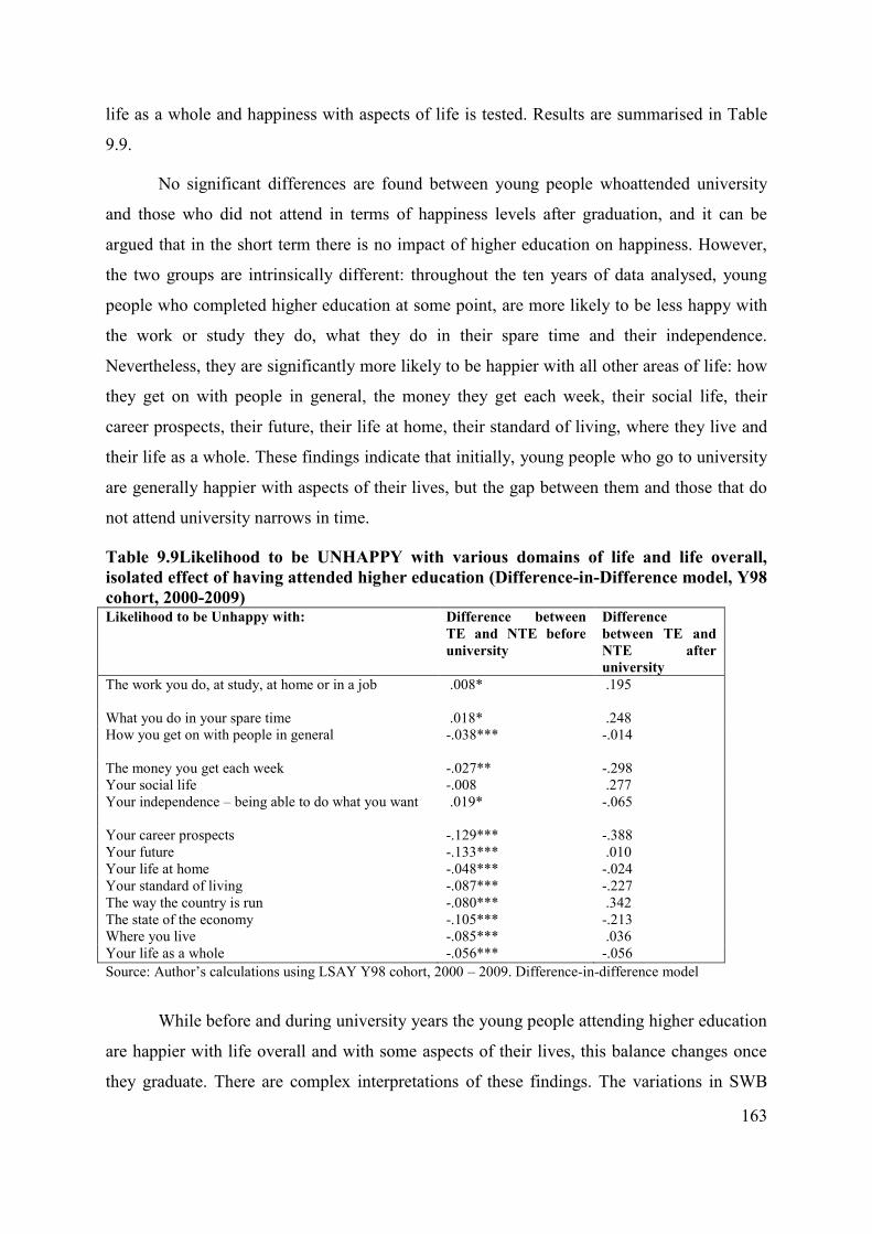
163
life as a whole and happiness with aspects of life is tested. Results are summarised in Table
9.9.
No significant differences are found between young people whoattended university
and those who did not attend in terms of happiness levels after graduation, and it can be
argued that in the short term there is no impact of higher education on happiness. However,
the two groups are intrinsically different: throughout the ten years of data analysed, young
people who completed higher education at some point, are more likely to be less happy with
the work or study they do, what they do in their spare time and their independence.
Nevertheless, they are significantly more likely to be happier with all other areas of life: how
they get on with people in general, the money they get each week, their social life, their
career prospects, their future, their life at home, their standard of living, where they live and
their life as a whole. These findings indicate that initially, young people who go to university
are generally happier with aspects of their lives, but the gap between them and those that do
not attend university narrows in time.
Table 9.9Likelihood to be UNHAPPY with various domains of life and life overall, isolated effect of having attended higher education (Difference-in-Difference model, Y98 cohort, 2000-2009) Likelihood to be Unhappy with: Difference between
TE and NTE before university
Difference between TE and NTE after university
The work you do, at study, at home or in a job .008* .195
What you do in your spare time .018* .248 How you get on with people in general -.038*** -.014
The money you get each week -.027** -.298 Your social life -.008 .277 Your independence – being able to do what you want .019* -.065
Your career prospects -.129*** -.388 Your future -.133*** .010 Your life at home -.048*** -.024 Your standard of living -.087*** -.227 The way the country is run -.080*** .342 The state of the economy -.105*** -.213 Where you live -.085*** .036 Your life as a whole -.056*** -.056 Source: Author’s calculations using LSAY Y98 cohort, 2000 – 2009. Difference-in-difference model
While before and during university years the young people attending higher education
are happier with life overall and with some aspects of their lives, this balance changes once
they graduate. There are complex interpretations of these findings. The variations in SWB

164
between those who opt into tertiary education and those who do not do so, may be attributed
to socio-economic variables, as well as to the different external factors affecting the two sub-
populations: those attending university are in a learning environment and those who do not
attend university enter the labour market. The stressors in the two situations are different and
psychologists argue that SWB is dependent on such stressors. The fact that the differences in
happiness overall and happiness with aspects of life disappear once the tertiary-educated
enter the labour market further support this argument.
Young people are a distinct cohort in that the items that add to their well-being are
different to those which those of the adult population, and furthermore, they are particularly
different as they find themselves in the school to work transition, a time of life-changing
events. The decisions to finish school, to enrol in tertiary education or to enter the labour
market are such life-changing events. As tertiary education is found to bring individual and
societal growth, it is important to explore whether all Australians have access to such
opportunities. The findings from this chapter conclude that although tertiary education has
become more accessible to young Australians in the past decade, there are still socio-
economic barriers to tertiary education and indirectly, to better life outcomes.
9.4 Conclusion
This chapter explored the subjective well-being during emerging adulthood (as discussed in
life-course theory, Santrock, 2007) using data from the LSAY survey. The levels of
happiness with areas of life and life overall have been explored in both cross-sectional
analysis of the Y06 cohort and longitudinal analysis of the Y98 cohort. Young people who
attend tertiary studies have been identified as less likely to be unhappy with the work they do,
at study, at home or in a job, with what they do in their spare time, with their social life, their
career prospects, their future and their life as a whole.
The longitudinal analysis explored education through two methods: as one possible
factor impacting happiness in a logit random effects model and by isolating the effect of
education in a pooled-OLS difference-in-difference model. This analysis also supports the
cross-sectional findings. Although there is no direct effect of having attended university, the
young people who attend tertiary education are not intrinsically less happy than other young
people. Hence lower levels of happiness at later points in life in the literature are intrinsic

165
characteristics of these individuals, but the unhappiness is ‘achieved’ along the life course.
An alternative explanation of the negative relation indentified by these studies is that the
measurement errors were embedded in the single-item indicator of SWB, generally used by
studies that explore the impact of education on SWB in multivariate models. This thesis
supports the latter explanation and its empirical evidence has been provided in Chapters 5, 6,
7 and 8.
Despite the objective and subjective outcomes streaming from the achievement of
tertiary qualifications, the case of well-being and tertiary education is not simple. In
Australia, attending tertiary education is not a choice equally available to all. Socio-economic
and demographic characteristics are factors impacting on tertiary education participation.
Students from disadvantaged backgrounds also face difficulties in completing school. It is
then recommended that education policies first be aimed at younger students to ensure school
completion, and, as a second step ease these young people’s paths towards and through
tertiary education.
166
Chapter 10 Discussion and conclusion
10.1 Thesis overview and key findings
In the well-being literature an association is commonly drawn between higher education
levels and higher economic development, better health, better employment opportunities, and
even happier marriages. Despite such objective outcomes, most studies of well-being have
identified a zero relationship between subjective well-being and higher educational
achievement, or even a negative one (Dockery, 2003; Headey and Wooden, 2004). Although
the number of studies addressing SWB has increased considerably in the past two decades,
few have attempted to explore the grounds for the non-positive relationship between tertiary
education and SWB.
In Australia too, most studies have found that having completed tertiary qualifications
does not increase individual subjective well-being (e.g. Hickson and Dockery, 2008).But
scholars using an exploratory approach to the relationship between education and SWB
underline the necessity for further empirical and theoretical examination of this paradox of
higher education and subjective well-being (the need for research in Australia is best
expressed by Dockery, 2010).
This thesis addressed this need for research through a quantitative exploration of the
SWB of tertiary-educated and non-tertiary-educated Australians using secondary data
sources. Three hypotheses were developed. The first hypothesis contradicted the paradox of
SWB and tertiary education. Drawing on human capital theory and the life-domain approach
to SWB, it said that the tertiary-educated are more satisfied with domains of life and with life
overall than the non-tertiary-educated. This hypothesis was both confirmed and refuted in
separate analyses in Chapter 5. When a single-item measure of SWB (overall satisfaction
with life) was explored, the tertiary-educated are found to be less satisfied with their lives
than the non-tertiary-educated. This refuted the hypothesis and confirmed the negative
relationship between SWB and tertiary educational achievement, or the paradox of SWB and
tertiary education. However, when the levels of satisfaction with particular domains of life
were compared, the tertiary-educated were found to be equally satisfied, or even more so,
than the non-tertiary-educated. Furthermore, when a multiple-item measure (or scale) was
used to calculate average satisfaction across all domains of life, the tertiary-educated were
identified as more satisfied with their lives. This finding suggests a positive relationship
between SWB and tertiary educational achievement. Because of the contradictory results
167
from the two methods –the single-item and the multiple-item measures of SWB – Chapter 5
concluded that an exploratory approach to the paradox was necessary.
The heterogeneity of SWB by tertiary-educational achievement is adopted as a
method of exploration. The second hypothesis of the thesis, that SWB is heterogeneous by
higher-educational achievement, was tested in Chapter 6. The thesis adopted the life-domain
approach and investigated whether all aspects of life were equally important to the tertiary-
educated and the non-tertiary-educated, using correlation and regression analyses. The
findings suggest that the tertiary-educated and non-tertiary-educated give different weights to
the various aspects of their lives, such as employment opportunities, finances and free time,
when assessing their overall well-being. Chapter 6 concluded that the tertiary-educated and
the non-tertiary-educated are heterogeneous groups in their conceptualisation of what counts
as their well-being, thus supporting the second hypothesis of the thesis.
The third hypothesis was that socio-economic and demographic factors do not have
the same impact on the satisfaction with domains of life and life-satisfaction of the tertiary-
educated and the non-tertiary-educated. This hypothesis was tested and supported through
regression analysis in Chapter 7.
The findings in Chapters 6 and 7 indicated that, when SWB is assessed through a
single-item measure such as ‘overall satisfaction, all things considered’, the tertiary-educated
and the non-tertiary-educated give different importance to aspects of their lives, and socio-
economic and demographic factors impact the conceptualisation of ‘what makes the good
life’ differently for the two sub-populations. These findings led to the conclusion that the
single-item measure of SWB carries conceptual biases, and that the multiple-item measure is
more reliable. This conclusion, triangulated with the findings in Chapter 5, allowed the thesis
to conclude that the tertiary-educated are more satisfied than the non-tertiary-educated, and
that there is no paradox of subjective well-being and tertiary education in Australia.
Drawing on findings from the literature reviewed, reflected in the analysis in Chapter
7, the thesis was also concerned with changes in perceptions of well-being due to age. The
third hypothesis said that SWB is heterogeneous by age, and that factors that impact on SWB
vary throughout stages of the life-course. This hypothesis was tested in Chapter 8 and only
partial confirmation was found. The chapter concluded that age matters to the
conceptualisation of well-being only in comparison between early and middle adulthood (25-
65 years) on the one hand, and late and very late adulthood (65 years and over) on the other.

168
This finding has the potential to explain the U-shaped relationship between SWB and age
found in the well-being literature. The analysis of the heterogeneity of SWB by stage of the
life-course indicated that, towards late and very late adulthood, conceptualisation of well-
being changes. This finding aligns the thesis with studies like Plagnol (2010) who pointed to
the crucial importance of perceptions when exploring SWB at later stages of life. Theories of
adaptation and of the shift in goals and stressors explain the variation in ‘what makes the
good life’ towards later stages of the life-course.
Finally, Chapter 9 explored the subjective well-being of young people, and how
tertiary education impacted on their well-being. The purpose of the chapter was twofold.
Firstly, it aimed to explore whether the tertiary-educated are inherently unhappy as some
studies have found. Secondly, it aimed to explore whether, under current educational policies,
access to tertiary education is equitable and all young people who wish to can afford to attend
tertiary education. The chapter found that young people who go to university are happier
before and during university years, but they become less happy than their counterparts who
opt out of education after school completion. The phenomenon was explained through
multiple discrepancies theory. The analysis of the most recent LSAY cohort data on tertiary-
education participation (2006-2009) revealed that, for some young people, factors like
financial disadvantage or remoteness are roadblocks to tertiary-education participation or
completion. Triangulated with the findings from previous chapters, these factors can also be
considered roadblocks to higher satisfaction with life, or higher well-being. The policy
implications of these findings are discussed in the next section.
The answer to the research question is that there is no paradox of subjective well-
being and tertiary education in Australia.The thesis concludes that, as well as the objective
advantages found in the well-being literature, tertiary-educational achievement is also
associated with higher subjective well-being.
10.2 Contribution to knowledge and methodological, theoretical and policy
prescriptions
The results challenge the well-being literature at both methodological and theoretical
levels. The methodological contributions are first discussed. The findings are then placed in
the context of the theoretical frameworks discussed in Chapter 2. The thesis also makes
policy recommendations.

169
10.2.1 Methodological connotations of the findings
The principal finding of the thesis and its contribution to knowledge is that there is no
paradox or puzzle of subjective well-being and tertiary education – the negative relationship
identified in the literature is driven by conceptual gaps in the traditional SWB measures. The
conceptual differences in the single-item measure of subjective well-being by higher
educational achievement have been demonstrated in Chapters 5, 6 and 7, allowing for the
conclusion that the findings summarised in Fig.10.1 are biased(not representing the reality),
while those in Fig.10.2are a better representation of SWB. These figures are reproduced
below from Chapter 5.
Fig.10.1 Average satisfaction with life 2001-2009 by education level
Source: Author’s calculations using HILDA 2001 – 2009.

170
Fig. 10.2 Overall satisfaction with life 2001-2009 by education level
Source: Author’s calculations using HILDA 2001 – 2009. Note: SWB was calculated as the arithmetic average of satisfaction with eight domains of life. Error bars are computed using the 2009 sample size.
The thesis also argued against some of the traditional methods to assess determinants
of well-being, such as multivariate analysis. This is because socio-economic and
demographic variables affect the SWB of the tertiary-educated and the non-tertiary-educated
to different degrees depending on the stage of the life course. Some of these findings are
worthy of note.
Conventionally, it is argued that women have higher levels of satisfaction, or
happiness, than men (e.g. Blanchflower and Oswald, 2008). Other studies have found that the
gender differences in subjective well-being depend on age (Inglehart et al., 2002). This thesis
also found that women during early adulthood (25-44 years)are more satisfied with their lives
than men. However, when the heterogeneity of SBW by higher-educational achievement was
accounted for, the effect of gender disappeared. That is, tertiary-educated women are not
more satisfied than tertiary-educated men, and non-tertiary-educated women are not more
satisfied that non-tertiary-educated men. This finding indicates that the conclusion that
women are more satisfied than men is driven by gender differences in populations with
different levels of education. During middle adulthood (45-64 years), non-tertiary-educated
women are more satisfied than non-tertiary-educated men. But the relationship does not apply
to tertiary-educated men and women, who are equally satisfied with their lives during middle
adulthood. During late adulthood there are no gender differences. During very late adulthood,

171
women are more satisfied than men overall, but the relationship is not statistically
significantwhen education is controlled for. The summative message is that gender
differences in terms of SWB diminish as individuals become highly educated.
This thesis also contributes to the debate on the impact of income on SWB. This
present research found that the impact of income depends on the type of income the
researcher includes in the multivariate model to explore determinants of well-being. The
impact of per person household equivalised income on the one hand, and the impact of own,
personal income on the other, were tested in Chapter 7, Section 7.2.8. Income quartiles were
calculated in each case. When testing the impact on well-being of equivalised income
quartile, the non-tertiary-educated in the first and second income quartile were less satisfied
with their lives than the non-tertiary-educated in the third income quartile. This finding
supports those studies which found that income had a limited impact on happiness or
satisfaction with life (for example Diener et al., 1999). The analysis in this thesis too,
concluded that household equivalised income increases satisfaction with life only to a certain
extent, up to the third income quartile. However, this is only the case for the non-tertiary-
educated. In the case of the tertiary-educated, only being in the bottom first quartile equates
to lower levels of SWB. As is the case with the impact of age and gender on SWB, the impact
of income on SWB loses significance for the tertiary-educated.
The results from above however only hold when the control for income is computed
as household equivalised income77. When personal income was used instead, the analysis
concluded that there is no significant impact of income on SWB for the non-tertiary-
educated. For the non-tertiary-educated, money does ‘bring happiness’, but only as long as it
is the household money (household equivalised income, which includes personal income and
the income of other household members), not own (personal) income. However, the impact of
personal income on the life satisfaction of the tertiary-educated is nearly identical to the
impact of household income: as long as the income is at the levels of the second income
quartile or above, income does not affect satisfaction with life. It can be argued that for the
tertiary-educated, the impact of income (either household equivalised or personal income)
77 As earlier explained in Chapter 4, both household equivalised income and own income have been used in
regression analyses. Household equivalised income was computed as the sum of own income of all household members divided by the square root of the number of persons in the household.

172
amounts to what Adam Smith’s described in The Wealth of Nations as ‘being able to go out
in public without shame’.
Finally, at the level of econometric modelling, this thesis explored the ‘participation bias’
identified by studies like Bell (1953) and Baird et al. (2010). This concept refers to the
phenomenon that one’s behaviour and perceptions of well-being are influenced by
participating in surveys of well-being for consecutive years. This bias was confirmed using
the HILDA data, and the calculations are presented in Appendix C. To avoid this bias, Baird
et al. (2010) recommend the use in SWB analyses of a panel design with refreshment
samples, instead of longitudinal, repeated data. For this reason, the models tested in the thesis
did not draw on the repeated cross-sectional data available in HILDA.
10.2.2 Theoretical implications
The theoretical framework of the thesis draws on concepts from multiple discrepancies
theory, life-course theory and stress research, life-span development, human capital theory
and the capabilities approach. The relevance of these theories for the exploration of the
relationship between SWB and tertiary education was discussed in Chapter 2. How the
findings of the thesis coincide with some of these theories is discussed in this section. The
capabilities approach and human capital theory are discussed in the policy recommendations
and included in Subsection 10.2.3.
Multiple discrepancies theory
The principles of multiple discrepancies theory, explained in Chapter 2, Section 2.2.1, are
well reflected in the findings of the thesis. The findings in Chapter 5illustrate this (see also
Figs. 10.1 and 10.2). Although there is a general tendency to overestimate overall satisfaction
(about half a point above average, see the figures above), the measures should not differ from
each other as they change over time, given that they reflect the same concept, SWB.
Furthermore, according to the life-domain approach, high satisfaction with domains of life
results in high overall satisfaction. However, this is not what happened (as shown in Chapter
5. Between 2001 and 2009 the average satisfaction of the non-tertiary-educated hardly
changed (variations of only 0.1), but the measure of their overall satisfaction followed a
decreasing trend. Similarly, while the average satisfaction of the tertiary-educated increased
throughout the nine years, the measure of their overall satisfaction did not change.

173
MDT principles can explain this unforeseen relationship between two measures of the
same concept. Levels of satisfaction with particular areas of life are closer representations of
reality than the overall measure. This is because, instead of being asked to assess how
satisfied they are ‘all things considered’, respondents are asked to focus on their satisfaction
with specific domains of life. Hence, differences in levels of satisfaction with areas of life of
the non-tertiary-educated and those of the tertiary-educated can be considered the
‘objectively measurable discrepancies’ (second principle of the MDT, see Chapter 2, Section
2.2.1 for complete discussion of this aspect of the theory). As shown in Fig. 10.1, since 2003
these discrepancies between the tertiary-educated and the non-tertiary-educated have
increased in favour of the tertiary-educated.
Furthermore, the first MDT principle states that net satisfaction (that is, overall
satisfaction) is a function of perceived discrepancies between, amongst others, what one
wants or has, and what others have (also discussed in Chapter 2, Section 2.2.1). The lower
levels of overall satisfaction of the non-tertiary-educated can then be attributed to these
discrepancies between their perceived well-being and the perceived well-being of the tertiary-
educated. Under the same thinking, the overall satisfaction of the tertiary-educated should
increase between 2001 and 2009, given the increase in their average satisfaction with
domains of life. However this is not the case, as the overall satisfaction of the tertiary-
educated did not change despite the increase in their average satisfaction with life. This
finding indicates first of all that these two MDT principles do not apply to tertiary-educated
individuals, reiterating the differences (or heterogeneity) of the two sub-populations.
Life-course theory
The application of the life-course theory to the exploration of the relationship between SWB
and tertiary educational achievement is limited, but not without significance. Chapter 8
concluded that the heterogeneity of SWB by stage of the life-course is limited. The levels of
overall satisfaction are similar for individuals aged 25-64 (early and middle adulthood) and
individuals older than 65 (late and very late adulthood). Nevertheless, when SWB was
explored over the life-course and by tertiary educational achievement, further differences
emerged: the heterogeneity of SWB by stage of the life-course reduces for the tertiary-
educated. It can be concluded that being tertiary-educated maintains older individualscloser
to the levels of well-being of younger individuals, including those in very late adulthood – at
least from the point of view of their perceptions of well-being.
174
Life-course theory however helps to explain the higher levels of overall life
satisfaction generally perceived by the older population, traditionally referred to as the
‘paradox of age and SWB’. Individuals older than 65 do not give the same weight to
satisfaction with domains of life as do individuals under 64 years. Other things ‘count’
towards the well-being of the former group. This indicates that a single measure of well-
being for individuals of all ages is not accurate.
10.2.3 Policy recommendations
The findings of the analysis connect mainly with two aspects of policy: well-being and
education.
SWB has become an item on the agenda of governments and multinational
organisations, equal in importance to aspects of quality of life such as health, work and life
balance, education, and social connections (OECD, 2011). However, SWB is a complex
concept and individuals give different weights to key aspects of life when assessing their
overall satisfaction. The thesis recommends that, in order to achieve higher levels of well-
being for all, policy makers should investigate those aspects of life important for the SWB of
target groups of individuals (e.g. low, medium and high income earners, or men and women).
Identifying ‘what counts’ for each group will allow for more efficient and cost-effective
policies to increase subjective and overall well-being by addressing the specific needsof
target groups.
Current governmental recommendations for education policy advise that by 2020, 40
per cent of Australians aged 25 to 39 years should have achieved tertiary qualifications
(Bradley Review, 2008).Triangulated with the findings of the thesis, that tertiary educational
achievement is associated with higher subjective well-being, this recommendation translates
to ‘by 2020 there should be higher subjective well-being and satisfaction with domains of life
for 40 per cent of Australians aged 25 to 39 years’. Reaching the goal set by the Bradley
Review would not only increase the international competitiveness of Australia from a labour-
market perspective, but also its national level of SWB.
However, there is a danger inequality may increase. Although Australia ranks
relatively high in terms of individuals’ SWB, compared with other OECD countries, some
economic inequalities are prominent (OECD, 2011). The thesis has found that a number of
young people from disadvantaged backgrounds do not have the material means to continue

175
their studies to tertiary level, and as such, given that higher education equates with higher
levels of SWB, they are being involuntarily kept in a ‘capped SWB zone’. Educational
policies facilitate the participation in tertiary education of disadvantaged young people
through measures such as the waiving of fees. However, this thesis has found that a large
proportion of young people who plan to go to university, for reasons outside their control do
not complete Year12, the minimal requirement for tertiary-education enrolment. Hence, one
of the recommendations of this thesis is that education policies aiming at increasing tertiary-
education participation and completion, should not only seek to ease the access to tertiary
education for those who have already completed Year12, but also seek to assure that students
are offered the opportunity to finish Year12. Helping out those who have already ‘made it’ to
Year12, and not supporting those who struggle against roadblocks to school completion, can
result in a widening of the inequality gap in Australia. The risk is a new generation where the
divisions between university graduates and individuals with under-Year12 education levels
are accentuated. Hence early intervention is necessary.
Although not the purpose of this thesis, other possible policy implications of the
findings can be flagged. Theories of adaptation such as the hedonic treadmill theory, set-point
theory or homeostatic theory argue that individuals tend to maintain constant levels of
subjective well-being, regardless of the events that occur in their lives. Some empirical
studies have found support for these theories. For example, Brickman and Coates (1978)
found that paraplegics are not less happy than individuals who can walk. However, the
analysis in Chapter 7 identified a negative effect of long-term illness on satisfaction with
aspects of life, as well as on overall satisfaction and average satisfaction. While further
analysis should be conducted to control for factors like the time since the onset of the illness
or disability, it can be concluded that in the context of disability and SWB in Australia such
adaptation theories do not apply. This finding flags a problem to policy makers, as population
with disabilities are not adequately integrated into society, being less satisfied than other
Australians with their employment opportunities, finances and accommodation (results of the
analysis are summarised in Chapter 7, Section 7.2.7) .
The comparison of levels of satisfaction with domains of life of the tertiary-educated
and the non-tertiary-educated in Chapter 5 revealed that the non-tertiary-educated are
constantly less satisfied with their health, a finding which was also previously identified in
the literature. Furthermore, the gap between the non-tertiary-educated and the tertiary-

176
educated has increased in the past decade, indicating possible problems in the health system
in Australia. Housing is another area where dissatisfaction was obvious from the analysis
(Chapter 5, Fig.5.7). Despite the usually higher incomes associated with tertiary education,
this group is less satisfied with their homes than the non-tertiary-educated. The satisfaction of
the latter group also decreased over time, indicating a general, overall dissatisfaction with
housing in Australia.
10.3 Limitations and further potential for research
A limitation of this study has been the lack of qualitative data collection. The reasons behind
having conducted a quantitative, secondary data analysis were discussed in Chapter 4.
Qualitative interviews with individuals who have completed tertiary education and those who
have not, and individuals of different ages, could however provide additional and in-depth
information on SWB. Governments have become interested in assessing national well-being
through indices of happiness or of personal well-being. However the items to be included in
such indexes are often a matter for debate. Qualitative interviews can contribute to the
computation of such national indices as they can reveal items of high importance to
individual well-being that would otherwise not be obvious to the researcher.
Various socio-economic and demographic variables such as gender, income or
geographic location can function as differentiating criteria within the heterogeneity approach
to subjective well-being78. The purpose of this thesis has been to explore the relationship
between SWB and tertiary education and for this reason the heterogeneous nature of SWB by
higher educational achievement was at the centre of the analysis. Age however was also
considered relevant to the analysis for several reasons. First, it is traditionally argued that
SWB follows a U-shaped trajectory throughout the life-course. The youngest and oldest are
argued to be happiest, or most satisfied with life (Frey and Stutzer, 2002; Blanchflower and
Oswald, 2004; Heady and Waren, 2008; Cummins, 2010). Second, the thesis identified a
strong impact of age on SWB in the Australian context. Third, the outcomes from education
are bound to change as individuals move from school to work, to the first years of
employment, to a career peak and so forth. For these reasons the paradox of SWB and tertiary
education was explored, first by addressing the heterogeneity of SWB by higher educational
78The heterogeneity of SWB by age, gender and education has been addressed by Rojas (2006), although only
absolute levels of satisfaction were compared without much investigation of possible conceptual differences in SWB.

177
achievement, and then a second layer of heterogeneity was added by accounting for four
stages of the life course (Elder, 1974).
The analysis revealed that aspects of life that count towards overall well-being lose
significance after the age of 65, and that there are differences between the tertiary-educated
and the non-tertiary-educated at each stage of the life course. It would be interesting to
further explore the well-being of the population over 65, inquiring about age-specific items
through the multiple-item measure of well-being. This would have particular applications to
aging studies and policies aiming to improve well-being after retirement. Similarly, the young
population (18-25 year olds) have youth-specific concerns, and their SWB should also be
addressed through age-specific questionnaires, such as those in LSAY. Some studies fail to
account for possible biases that the younger and the older population may draw on the overall
results. These problems should not be overlooked as the population aged 18 to 25 years,
together with those aged over 65, represent a third of the adult population (33.4 per cent in
Australia, Chapter 4, Table 4.1, author’s calculations using HILDA 2009).
Identifying methodological concerns with the assessment of SWB through single-item
or multiple-item measures raises further questions of the accuracy of these measures in the
context of this thesis and in SWB research in general. The author recommends that the
relationship between SWB and higher education is further explored using other alternative
measurements of SWB such as experiences of positive and negative affect. This approach has
explored by Kahneman and Krueger (2006), who examined well-being through the day
reconstruction method, asking individuals to recollect memories of the previous day by
writing a short diary. Its application is new but there is great potential for exploration in the
context of – already traditional – puzzles such at the impact of income, age or education on
‘happiness’.
Although collecting longitudinal data is problematic and time-consuming, a between-
group comparison of experiences of positive and negative affect throughout the day is
recommended. It could be useful to explore whether the experience of positive and negative
affect during activities throughout the day is heterogeneous by higher educational
achievement, and to what extent the age factor influences the results. Cross-national
comparisons couldalso be useful to assess the value higher education adds to private lives in
various cultural and economic contexts. While such data is available for countries like the

178
United States (the Princeton Affect Time Survey), the need for such a collection of data has
recently been gaining prominence in Australia.

179
References
Argyle, M. (1987). The Psychology of Happiness, Routledge, London, 1987.
Argyle, M. (2001).The psychology of happiness, (2nd ed.). London.
Arnett, J. J. (2000). Emerging Adulthood: A theory of development from the late teens through the twenties, American Psychologist, 55(5), 469-480.
Baird, M., Lucas, R.E. and Donnellan, M.B. (2010). Life Satisfaction Across the Lifespan: Findings from Two Nationally Representative Panel Studies, Social Indicators Research, 99, 183-203.
Baltes, P. B. (1968). Longitudinal and cross-sectional sequences in the study of age and generation effects. Human Development, 11, 145-171.
Bauer, R. A. (1966). Social Indicators. Cambridge, Mass. MIT Press.
Becker, G. S. (1964). Human capital. New York: Columbia University Press.
Bell, R, Q. (1953). Convergence: An accelerated longitudinal approach. Child Development, 24, 145-152.
Bennett, N.G., Bloom, D.E. and Craig, P.H. (1989).The Divergence of Black and White Marriage Patterns, Discussion Papers 1989(22), Columbia University, Department of Economics.
Bjørnskov, C., Dreher, A., and Fischer, J.(2007).On Gender Inequality and Life Satisfaction: Does Discrimination Matter? Working Paper Series in Economics and Finance 657, Stockholm School of Economics.
Blanchflower, D. G., 2001. Unemployment, Well-Being, and Wage Curves in Eastern and Central Europe, Journal of the Japanese and International Economies, 15(4), 364-402.
Blanchflower, D. G. and Oswald, A. J. (1994).
Blanchflower, D. G. and Oswald, A. J. (2004).Well-being over time in Britain and the USA, Journal of Public Economics,vol88, 1359–1386.
Blanchflower, D. G.and Oswald, A. J. (2007/2008). Is Well-being U-Shaped over the Life Cycle?, NBER Working Papers 12935, National Bureau of Economic Research, Inc.
Blau, F. D. (1998).Trends in the Well-Being of American Women, 1970-1995,Journal of Economic Literature, 36(1), 112-165.
Blonna, R. (2007). Coping with stress in a changing world, McGraw-Hill Publishing Company.
Boslaugh, S. (2007). Secondary Data Sources for Public Health, Cambridge.
Bradbury, R. E. (1969). In Douglas, M., and Kaberry, Ph. M. (eds.), Man in Africa (pp. 17–36). London
Bradley, D., Noonan, P., Nugent, H. and Scales, B. (2008). Review of Australian Higher Education ‘The Bradley Review’, Final Report. Australian Government.
Bradshaw, J., Hoelscher, P. and Richardson, D. (2006) Comparing Child Well-being in OECD Countries: Concepts and Methods, Innocenti Working Paper, Unicef.

180
Bradshaw, J. and Richardson, D. (2009) An Index of Child Well-Being in Europe, Child Ind Res, 2, 319-351.
Bradshaw, J. and Keung, A. (2011) Subjective well-being and mental health, in J. Bradshaw (ed.) The Well-being of Children in the UK, 3rd ed., The Policy Press, Bristol, pp.89-109. Brickman, P.D. and Campbell, D.T. (1971).‘Hedonic relativism and planning the good
society’ in M.H. Appley ed. Adaptation Level Theory. New York: Academic Press.
Brickman, P.D., Coates, D. and Janoff-Bulmann, R. (1978). Lottery winners and accident victims: is happiness relative? Journal of Personality and Social Psychology, 36, 917-27.
Bruni L. and P. L. Porta (eds.). (2006). Economics and Happiness: Framing the Analysis, New York: Oxford University Press.
Campbell, A. (1981). The Sense of well-being in America. McGraw-Hill, New York.
Campbell, A. and Converse, P. E. (1972). The Human Meaning of Social Change, New York: Russell Sage Foundation.
Campbell, A., Converse, P. E. and Rodgers, W. L. (1976).The Quality of American Life.New York. Russell Sage.
Cantril, H. (1965). The pattern of human concerns. New Brunswick, NJ: Rutgers University Press.
Casas F, Figuer C, González, M. and Coenders, G. (2004) Satisfaction with Life Domains and Salient Values for Future: Data from Children and their Parents in Five different Countries. In Glatzer, W., Below, S. and Stoffregen, M. (Eds.) Challenges for Quality of Life in the Contemporary World. Advances in Quality-of-Life Studies, Theory and Research, pp233-247.
Casas, F., Figuer, C., Gonzalez, M., Malo, S. Alsinet, C. and Subarroca, S. (2007). The Well-Being of 12-to-16-year-old Adolescents and their parents. Results from 1999 to 2003 Spanish Samples, Social Indicators Research, 83(1), 87-115.
Clark, A. E. (1996). Women's wellbeing at work,New Economy, Institute for Public Policy Research, 3(1), 25-28.
Clark, A. E. and Oswald, A. J.(1994).Unhappiness and Unemployment, Economic Journal, Royal Economic Society, vol. 104(424), 648-59.
Clark, A. E. and Oswald, A. J.(1996). Satisfaction and comparison income, Journal of Public Economics, 61(3),359-381.
Clark, A.E. (2007). Born To Be Mild? Cohort Effects Don’t (Fully) Explain Why Well-Being Is U-Shaped in Age, IZA Discussion Papers 3170, Institute for the Study of Labor (IZA).
Clark, A., Etilé, F., Postel-Vinay, F., Senik, C. and Van der Straeten, K. (2005).Heterogeneity in Reported Well-Being: Evidence from Twelve European Countries, Economic Journal, 115, 118-132.
Clark, A.E., Frijters, P., and Shields, M. A.(2008). Relative Income, Happiness, and Utility: An Explanation for the Easterlin Paradox and Other Puzzles, Journal of Economic Literature, 46(1), 95-144.

181
Cohen, S., and Edwards, J. R. (1989). Personality characteristics as moderators of the relationship between stress and disorder. In W. J. Neufeld (Ed.), Ad00vances in the investigation of psychological stress (235-283). New York: Wiley.
Cottam, Howard R. (1941). Methods of Measuring Level of Living, Social Participation and Adjustment of Ohio Farm People, Methodological Supplement to the Agricultural Experiment Station Bulletin No. 624,Columbus, Ohio: Ohio State University and Ohio Agricultural Experiment Station, July. (Mineo.)
Cottam, Howard R.: Mangus, A. R. (Dec., 1942). A Proposed Definition of the Standard of Living. Social Forces, Vol. 21, No. 2, 177-179. Costa, P.T. and McCrae, R.R.(1980). Influences of extraversion and neuroticism on
subjective well-being, Journal of Personality and Social Psychology, 38, 668-78.
Craig, L., Mullan, K. and Blaxland, M. (2010).Parenthood, Policy and Work-Family Time in Australia 1992—2006.Work, Employment & Society 24(1), 27 - 45.
Christoph B. and Noll, H. H. (2003). Subjective Well-being in the European Union During the 1990ies. Social Indicators Research, 64, 521-546
Crosby, F. J. (1982). Relative deprivation and working women, Nueva York, EUA: Oxford University.
Cummins, R.A. (1995). On the trail of the gold standard for life satisfaction, Social Indicators Research, 35, 179-200.
Cummins, R. (1996). The Domains of Life Satisfaction: An Attempt to Order Chaos, Social Indicators Research, 303-328,
Cummins, R. (1997).Comprehensive Quality of Life Scale - Adult, Deakin, Melbourne.
Cummins, R. (1998).Directory of instruments to measure quality of life and cognate areas.4th ed., 1-88, School of Psychology, Deakin Univ, Melbourne.
Cummins, R. (2000). Objective and Subjective Quality of Life: an interactive model.,Social Indicators Research, 55-72.
Cummins, R. A. (2002) The validity and utility of subjective quality of life: a reply to Hatton and Ager, Journal of applied research in intellectual disabilities, vol. 15, no. 3, pp. 261-268, Blackwell Publishers, Oxford, England
Cummins, R. A., Eckersley, R., Pallant, J., van Vugt, J. and Misajon, R. (2003) Developing a national index of subjective wellbeing: the Australian unity wellbeing index, Social indicators research, vol. 64, no. 2, pp. 159-190, Reidel Pub. Co, Dordrecht, Netherlands
Cummins, R. A. (2006) Australian Unity wellbeing index : fifth anniversary special report, Deakin University, Geelong, Vic.
Cummins, R. A. (2010). Subjective wellbeing, homeostatically protected mood and depression: a synthesis, Journal of happiness studies, 11( 1), 1-17.
Desjardins, R. (2008). Researching the Links between Education and Well-being. European Journal of Education. Special Issue: Education and Well-being, 43 (1), 23-35.
Di Tella, R, MacCulloch R. J., and Oswald. O. J. (2001). Preferences over Inflation and Unemployment: Evidence from Surveys of Happiness. American Economic Review ,91(1), 335-341.

182
Diener, E. (1984) Subjective well-being. Psychological Bulletin, 95, 542-575.
Diener, E. (1999). Introduction to the special section on the structure of emotion. Journal of Personality and Social Psychology. 76, 803-804.
Diener, E. and Diener, C. (1995). Most Poeple are Happy, Psychological Science, 7(3), 181-185.
Diener, E., Diener, M., and Diener, C. (1995).Factors predicting the subjective well-being of nations. Journal of Personality and Social Psychology, 69, 851–864.
Diener, E., Emmons, R. A., Larson, R. J. and Griffin, S. (1985). The satisfaction with life scale. Journal of Personality Assessment. 49, 71-75.
Diener, E. and Lucas. E. (1999). Personality and subjective well-being in Kahneman, D.. Diener, E., Schwarz. N (Ed). Well-being: The foundations of hedonic psychology, New York, NY, US. Russell Sage Foundation. 213-29.
Diener, E., Suh, E. M., Lucas, R. E. and Smith, H. E. (1999). Subjective well-being: Three Decades of Progress, Psychological Bulletin, 125, 276-302.
Diener, E., Lucas, R.E. and Scollon, C. (2006). Beyond the hedonic treadmill: revising the adaptation theory of well-being, Psychological Science, 61, 305-314.
Diener, E. and Suh, E.(1997).Measuring quality of life: Economic, social subjective indicators.Soc. Indic. Res., 40, 189-216.
Diener, E., Suh, E. M., Lucas, R. E. and Smith, H.L. (1999) Subjective Well-being: Three Decades of Progress. Psychological Bulletin, 125, 276 – 302.
Dockery, A. M. (2003). Happiness, life-satisfaction and the role of work: Evidence from two Australian surveys, paper presented at Curtis Business School.
Dockery, A. M. (2010). Education and happiness in the school-to-work transition, NCVER Research Report, item no 2239, ISBN 9781921413865.
Dolan, P., Peasgood, T. and White, M. (2007). Do we really know what makes us happy? A review of the economic literature on the factors associated with subjective well-being. Journal of Economic Psychology, 29 (2008), 94-122.
Easterlin, R. A. (1974). Does Economic growth improve the human lot? Some empirical evidence. In P.A. David and M.W. Redereds. Nations and households in economic growth pp. 89-125). New York: Academic Press.
Easterlin, R.A.(1995). Will raising the incomes of all increase the happiness of all?,
Journal of Economic Behavior and Organization, 27(1), 35–48.
Easterlin, R. A. (2004). The Economics of Happiness. Daedalus 133(2), 26-33.
Easterlin, R. A. (2005). ‘Building a better theory of well-being’ in L. Bruni and P. Porta eds. Economics and Happiness: Framing the Analysis. Oxford: Oxford Univ. Press.
Easterlin, R. A. (2007). The Escalation of Material Goals: Fingering the Wrong Culprit, Psychological Inquiry, 18(1), 31-33.
Elder, G. H., Jr. (1974).Children of the Great Depression. Chicago: University of Chicago Press.

183
Elder, G. H., Jr. (1998).The Life Course as Developmental Theory. Child Development. 69:1–12.
Erikson, R. (1993). Descriptions of Inequality: The Swedish Approach to Welfare Research. In: M. Nussbaum, A. Sen (eds.), The Quality of Life. Oxford: Clarendon Press, 67-87.
Farquhar, M.G. (1995). Elderly people’s definitions of quality of life. Soc. Sci. Med., 41: 1439-1446.
Feinman, S. (1978). The Blind as “Ordinary People”, Journal of Visual Impairment and Blindness (72-6), 231-38
Fernandez, E. A. (2010). SOCW1003 Human Behaviour1, Life Stress and the Life Span. UNSW
Ferriss, A.L. (20xx) The quality of life concept in sociology, The American Sociologists, 35 (3), 37-51.
Frey, B. S. and Stutzer, A. (2002) Happiness and Economics. Princeton University Press, Princeton, N.J.
Frijeters, P. And Beatton, T. (2008).The mystery of the U-shaped relationship between happiness and age. National Centre for Econometric Research Working Paper Series.
Gasper, D. (2010).Understanding the diversity of conceptions of well-being and quality-of-life.Journal of Socio-Economics, 39, 351-360.
Gerdham, U. G. and Johannesson, M. (1991). The relationship between happiness, health and socio-economic factors: results based on Swedish micro data, The Journal of Socio-Economics, 30(6), 553-557
Gong, C., Casselsl, R., and Keegan, M. (2011).Understanding life satisfaction and the education puzzle in Australia: A profile from HILDA Wave 9. NATSEM Working Paper 11/12.
Giele, J. Z., and Elder, G. H., Jr. (1998).Methods of Life Course Research: Qualitative and Quantitative Approaches. Thousand Oaks, CA: Sage.
Haas, B. K. (1999) A Multidisciplinary Concept Analysis of Quality of Life, Western Journal of Nursing Research, 21 (6), 728-742.
Hagood, M. J., Danilevsky, N., and Beum, C.O. (1941).An Examination of the Use of Factor Analysis in the Problem of Subregional Delineation, Rural Sociology 6 (3), 216-235.
Hartog, J.and Oosterbeek, H. (1998). Health, wealth and happiness: why pursue a higher education? Economics of Education Review, vol. 17(3), 245-256.
Hartog, J. and van den Brink, H. M. (2007).Human Capital: Advances in Theory and Evidence, Cambridge University press.
Hayward, K., L. Pannozzo and Colman, R.(2005).Draft: Developing Indicators for theEducated Populace Domain of the Canadian Index of Wellbeing, Interim Report,GPI Atlantic, Halifax.
Headey, B. (1988). The life satisfactions and priorities of Australians. Pps 163-175 in Jonathan Kelley and Clive Bean (Editors). Australian Attitudes: Social and Political Analyses from the National Social Science Survey. Sydney: Allen and Unwin.

184
Headey, B. (2006) Happiness: Revising set point theory and dynamic equilibrium theory to account for long term change. Discussion paper no. 607. DIW Berlin, German Institute for Economic Research.
Headey, B. (2010). The Set Point Theory of Well-Being Has Serious Flaws: On the Eve of a Scientific Revolution? Social Indicators Research, 97, 7-21.
Headey, B., Muffels, R. J. A. and Wagner, G. (2010). Long-running German panel survey shows that personal and economic choices, not just genes, matter for happiness. Proceedings of the Academy of Sciences 107 (42), 17922-17926.
Headey, B., Muffels, R.J.A., and Wagner, G. (2011).Choices which change life satisfaction: Similar results for Australia, Britain and Germany. SOEP Papers, 302.
Headey, B. W., Muffels, R. J. A., and Wooden, M.(2004). Money Doesn’t Buy Happiness - or Does It? A Reconsideration Based on the Combined Effects of Wealth, Income and Consumption, IZA Discussion Papers 1218, Institute for the Study of Labor (IZA).
Headey, B., Veenhoven, R. and Wearing, A. (1991). Top-down versus bottom-up theories of subjective well-being, Social Indicators Research, 24(1), 81-100.
Headey, B.W. and Wearing, A. J. (1992). Understanding Happiness: A Theory of Subjective Well-Being. Melbourne: Longman Cheshire.
Headey, B. W. and Wearing, A. J. (2010). Coping with the Social Environment: The Relationship Between Life Events, Coping Strategies and Psychological Distress, Australian and New Zealand Journal of Public Health, 12(4), 444-452.
Headey, B. and Warren, D. (2008), Families, Incomes and Jobs, Volume 3: A Statistical Report on Waves 1 to 5 of the HILDA Survey, Melbourne institute of Applied Economic and Social research, University of Melbourne.
Headey, B. and Wooden, M. The Effects of Wealth and Income on Subjective Well-being and Ill-being, The Economic Record 80, September 2004, Special Issue, pp. S24-S33.
Helliwell, J. F. (2003). How’s life? Combining individual and national variables to explain subjective well-being. Economic Modelling, 20(2), 331-360.
Hickson, H and Dockery, A. (2008).Is ignorance bliss? Exploring the links between education, expectations and happiness. Australian conference of economists, edited by KhorshedAlam, 1-24, Brisbane, Queensland, Australia: Economic Society of Australia (Queensland) Inc, 2008.
van Hoorn, A. (2007). A Short Introduction to Subjective Well-Being: Its Measurement, Correlates And Policy Uses. Paper at the Is happiness measurable and what do those measures mean for policy? 2-3 April 2007, Italy.
Hyde, M, Wiggins, R. D. and Blane, D. B. (2003). A measure of quality of life in early old age: The theory, development and properties of a needs satisfaction model (CASP-19). Aging and Mental Health, 7(3), 186-194.
Inglehart, R. F. (1977). The silent revolution: Changing values and political styles among Western publics. Princeton University Press, Princeton, N.J.
Inglehart, R. (1990).Culture Shift in Advanced Industrial Societies, Princeton University Press, Princeton, N.J.

185
Inglehart, R. F., Norris, P. and Welzel, C. (2002).Gender Equality and Democracy. Comparative Sociology, 1(3/4), 321-346.
Joshson, D. R. and Wu, J. (2002). An empirical test of crisis, social selection, and role explanations of the relationship between marital disruption and psychological distress; A pooled time series analysis of four-wave panel data. Journal of Marriage and the Family 64, 211-24.
Juster, F.T. (1985). Preferences for work and leisure. In Time, goods, and well-being. Ed. F.T. Juster and F.P. Stafford, 333-51. Ann Arbor, MI: Institute for Social Research, University of Michigan.
Kahneman, D. (1999). Objective happiness. In D. Kahneman, E. Diener and N. Schwarz (Eds.) Wellbeing: the foundations of hedonic psychology (pp. 3-25). New York: Russell Sage.
Kahneman, D. and A.B. Krueger (2006).Developments in the measurement of subjective well-being. Journal of Economic Perspectives, 20(1):3-24.
Von dem Knesebeck, O. (2007). Socio-economic position and quality of life among older people in 10 European Countries, Ageing society, 27(2), 269-284.
Von Dem Knesebeck, O., Hendrik, J., Borsch-Supan, A. (2007). Quality of work, well-being, and intended early retirement of older employees – baseline results from the SHARE study. European Public Health Association vol.17 issues 1 2007, 62-68.
Krueger, A., Kahneman, D., Schkade, D., Schwarz, N. and Stone, A. (2009).National Time Accounting: The Currency of Life, draft paper, 2008.
Krueger, A., Kahneman, D., Schkade, D., Schwarz, N. and Stone, A. (2009).National Time Accounting: The Currency of Life, in A. Krueger (Ed.) Measuring the Subjective Well-Being of Nations: National Accounts of Time Use and Well-Being
Kutner, B., Fanshel, D., and Togo A. (1956) Self image scale, Clinical and social psychology, 269-296.
Langlois, A. and Anderson, D. E.(2002).Resolving the quality of life/well-being puzzle: Toward a New Model. Can. J. Region. Stud., 35: 1-10.
Lazarus, R. S., and Folkman, S. (1984). Stress, Appraisal, and Coping. New York: Springer.
Lee, G., Secombe, K., and Shehan, C. (1991). Marital status and personal happiness: An analysis of trend data. Journal of Marriage and the Family, 53, 839-844.
Leu, R. E., Burri, S., and Priester, T. (1997), Lebensqualität und Armut in der Schweiz, Bern-Stuttgart-Wien: Verlag Paul Haupt.
Lleras-Muney, A. (2005). The Relationship Between Education and Adult Mortality in the United States. Review of Economic Studies 72,189-221.
Lochner, L. and Moretti, E. (2003).The Effect of Education on Crime: Evidence from Prison Inmates, Arrests, and Self-Report.
Long, M., Carpenter, P. and Hayden, M. (1999), Participation in education and training 1980-1994. LSAY Research Report No. 13. Melbourne: ACER.

186
Lucas, R. E., Clark, A. E., Georgellis, Y. and Diener, E. (2003). Reexamining Adaptation and the Set Point Model of Happiness: Reactions to Changes in Marital Status. Journal of Personality and Social Psychology 84 (3), 527-39.
Lykken, D. and Tellegen, A. (1996). Happiness is a stochastic phenomenon. Psychological Science, 7, 186-89.
Lyngstad, T. H. (2005) Why do Couples with Highly Educated Parents have Higher Divorce Rates? European Sociol Rev 22(1), 49-60.
Magnus, K., Diener, E. Fujita, F., and William, P. (1993). Extraversion and Neuroticism as Predictors of Objective Life Events: A longitudinal analysis. Journal of Personality and Social Psychology 65(5).1046-1053.
Marginson, S. (1993) Education and Public Policy in Australia, Melbourne/Cambridge: Cambridge University Press.
Marginson, S. And Considine, M. (2000) The Enterprise University: Power, Governance and Reinvention in Australia, Melbourne/Cambridge: Cambridge University Press.
Marginson, S., Nyland, C., Sawir, E. and Forbes, Mewett, H. (2010) International Student Security, Melbourne/Cambridge: Cambridge University Press.
Marks, G.N., Fleming, N., Long, M. and McMillan, J. (2000).Patterns of Participation in Year 12 and Higher Education in Australia: Trends and Issues, Longitudinal Surveys of Australian Youth Research Report. No. 17, Australian Council for Educational Research, Melbourne.
Marks, G.N. (2007). Income Poverty, Subjective Poverty and Financial Stress, Australian Government Social Policy Research Paper No.29, June 2007.
Martin Report (1964). The Commonwealth Government.
Mastekaasa, A. (1994). Marital status, distress, and well-being: An international comparison. Journal of Comparative Family Studies, 25, 183-205.
McKain, W. C. Jr. (1939). The Concept of Plane of Living and the Construction of Plane of Living Index, Rural Sociology 4: 337-343.
Meadow H. L., Mentzer, J. T., Rahtz, D. R. and Sirgy M. J. (1992) A Life Satisfaction Measure Based on Judgment Theory, Social Indicators Research 26, 23-59. Michalos, A.C. (1985). Multiple discrepancies theory, Social Indicators Research, 16, 347-
413.
Michalos, AC 2007, Education, happiness and wellbeing, paper written for the International Conference on ‘Is happiness measurable and what do those measures mean for public policy?’, University of Rome, April.
Miller, P. W. (2005). Under-education and Over-education in the Australian Labour Market, Economic Record (81), Issue Supplement s1, S22-S33.
Milligan, K., Moretti.E. and Oreopoulos, P.(2004). Does education improve citizenship? Evidence from the United States and the United Kingdom. Journal of Public Economics, 88(9-10), 1667-1695.
Mincer, J. (1974). Schooling, experience, and earnings. New York: Columbia University Press.

187
Moller, V. and Saris, W. E. (2001). The Relationship Between Subjective Well-Being and Domain Satisfaction in South Africa, Social Indicators Research 50, 187-208.
Muffels, R. and B. Headey (2009).Testing Sen’s capability approach to explain objective and subjective well-being using German and Australian Panel Data? Paper at the HILDA Survey Research Conference 2009, 16-17 July, Melbourne.
Myers, D. M. (1992).The pursuit of happiness. New York:Morrow.
Myrskyla, M. and Margolis, R. (2012). Happiness: Before and After the Kids. Max-Planck-Institute for Demographic Research
Newman, L. (2000). Social research methods: qualitative and quantitative approaches, London: Allyn and Bacon.
Noll, H. H. (2000) in Genov, Nicolai Ed. (2002) Advances in Sociological Knowledge over Half a Century. Paris: International Social Science Council.
Noll, H. H. (2006). European Survey Data: Rich Sources for Quality of Life Research. Paper presented to the ISQOLS Conference ‘Prospects for Quality of Life in the New Millennium’. Rhodes University, 17-20 July.
Nussbaum, M. C. (2000) Women and Human Development: The Capabilities Approach Cambridge University Press. Cambridge.
Nussbaum, M. C. (2007). On Moral Progress: A response to Richard Roty, The University of Chicago Law Review, 74(3), 939-960.
Okun, M. A., and George, L. K. (1984).Physician- and self-ratings of health, neuroticism and subjective well-being among men and women. Personality & Individual Differences, 5, 533-539.
OECD (2011). How’s life? Measuring well-being, Better Life Initiative.
Oswald, A. J. (1997). Happiness and economic performance. Economic Journal, 107, 1815-1831.
Oswald, A. J. and Powdthavee, N. (2007). Death, Happiness, and the Calculation of Compensatory Damages, IZA Discussion Papers3159, Institute for the Study of Labor (IZA).
Pearlin, L. I. And Skaff, M. M., 1996 Stress and the Life Course: A paradigmatic Alliance, The Gerontologist, 36(2), 239-247.
Peiro, A. (2006). Happiness, satisfaction and socio-economic conditions: Some international evidence. Journal of Socio-Economics, vol.35(2), 348-365.
Phillimore, J. and Koshi, P. (2010). Implications of the proposed low SES participation target for Australian University Enrolment. Final Report. Curtin University of Technology.
Pinquart, M. and Sorensen, S. (2001). How effective are psychotherapeutic and other psychosocial interventions with older adults? A meta-analysis. Journal of Mental Healthand Aging, 7, 207–243.
Plagnol, A. C. (2010). Subjective well-being over the life course: Conceptualizations and evaluations. Social Research: An International Quarterly. 77(2), 749-768.

188
Plagnol, A. C. and Scott, J. (2008). What matters for well-being: Individual perceptions of quality of life before and after important life events. Applied Research in Quality of Life. 6(2), 115-137.
Van Praag, B. M. S., Frijters, P. and Ferrer-i-Carbonell, A. (2003). The Anatomy of Subjective Well-Being, Journal of Economic Behavior and Organization, 51, 29-49.
Van Praag, B. M. S. and Ferrer-i-Carbonell, A. (2004). Happiness Quantified: A Satisfaction Calculus Approach. Oxford: Oxford University Press.
Preedy, V.R and Watson, R. R. (2010).Handbook of disease burdens and quality of life measures. Springer New York, New York.
Qian, Z. and Preston, S.H. (1993). Changes in American Marriage, 1972–1987: Availabililty and Forces of Attraction by Age and Education. American Sociological Review 58, 482-95.
Raimo, J. M., Bumpass, L. and Iwasawa, M. (2004). Marital Dissolution in Japan: Recent Trends and Patterns, Demographic Research, 11, 395-420.
Ramia, G., Marginson, S., Sawir, E. and Nyland, C. (2011) Global Business and Economics Review.13(2), 105-125.
Rapley, M. (2003), Quality of Life Research. A Critical Introduction. Sage Publications.
Reid, C. and Ponic, P. (2004). Living in isolations: women’s experience of poverty and exclusions. Friends of women and children in B.C, 3(10), 1-4.
Rojas, M. (2004).The Complexity of Well-being. A Life Satisfaction Conception and a Domains-of-Life Approach. Paper or the International Workshop on Researching Well-being in Developing Countries, Hanse Institute for Advanced Study, 2-4th July 2004.
Rojas, M. (2006).Life satisfaction and satisfaction in domains of life: is it a simple relationship?, Journal of Happiness Studies, Springer, vol. 7(4), pages 467-497, November.
Rojas, M. (2006). The Utility of Happiness Research in Economics, Journal of Happiness Studies, Springer, vol. 7(4), pages 523-529, November.
Rose, E. (2003) Does Education Really Disadvantage Women in the Marriage Market? Working Paper No.33, Center for Statistics and the Social Sciences, University of Washington.
Ross, C. E. and Van Willigen, M. (1997).Education and the Subjective Quality of Life. Journal of Health and Social Behavior38, 275-297.
Ryff, C. D. (1989). ‘Happiness is Everything, or Is It? Explorations on the Meaning of Psychological Well-Being’, Journal of Personality and Social Psychology, 57, 1069-1108.
Saito, M. (2003).Amartya Sen’s Capability Approach to Education: A Critical Exploration. Journal of Philosophy of Education.37 (1), 17-33.
Santrock, J. W. (2007). A topical approach to life-span development. Fourth Edition. McGraw-Hill Humanities/Social Sciences/Languages.
Scott, J. (2008). Changing Gender Roles in Scott, J. et al Women and Work: Changing Lives and New Challenges, Edward Elgar, p156-178.

189
Sen, A. K. (1985) Commodities and Capabilities, Amsterdam. North Holland, reprinted by Delhi, Oxford University Press.
Sen, A. K. (1987).The Standard of Living. Cambridge University Press. Cambridge.
Sen, A. K. (1993). Capability and Well-being in: Nussbaum and Sen (eds), 31–53.
Sen, A. (1999). Development as Freedom. New York: Anchor Books.
Sewell, William H. 1940. The Construction and Standardization of a Scale for the Measurement of the Socioeconomic Status of Oklahoma Farm Families, Technical Bulletin No. 9, Stillwater, Oklahoma: Oklahoma Agricultural Experiment Station.
Schaie, K. W. (1965). A general model for the study of developmental problems. Psychological Bulletin, 64, 92-107.
Schuessler, K. F. and Fisher, G. A. (1985).Quality of Life Research and Sociology. Ann. Rev. Sociol.(11), 129-49.
Sharpe, J. P., and Gilbert, D. G. (1998).Effects of repeated administration of the Beck depression inventory and other measures of negative mood states, Personality and Individual Differences, 24, 457-463.
Shin., D. and Johnson, D. (1978).Avowed happiness as an overall assessment of the quality of life. Social Indicators Research, 5, 475-492.
Schults, T. W. (1960). Capital formation by education. Journal of Political Economy, University of Chicago Press, 68,571.
Schultz, T.W. (1971).Investment in Human Capital. New York. The Free Press.
Smith, A. (2003, first published in 1776) The Wealth of Nations. Bantam USA.
Smith, D. (1973) The Geography of Social Well-Being in the United States, Mcgraw-Hill, New York.
Steering Committed for the Review of Government Service Provision (2011). Overcoming Indigenous Disadvantage. Key Indicators 2011, Commonwealth Australia.
Stevenson, B., and Wolfers, J. (2008). Economic growth and subjective well-being: Reassessing the Easterlin Paradox. Brookings Papers on Economic Activity, 1–102.
Stiglitz, J. E., Sen, A. and Fitoussi, J. P. (2009).Report by the Commission on the Measurement of Economic Performance and Social Progress. OECD.
Stutzer, A. (2003).Income aspirations, subjective well-being and labour supply. Paper presented at the ESF Exploratory Workshop ‘’Income Interactions and Subjective Well-Being, Paris, 25–26 September.
Stutzer, A. (2004).The Role of Income Aspirations in Individual Happiness. Journal of Economic Behaviour and Organization, 54 (1), 89 - 109.
Stutzer, A and Frey, B. S. (2010).Recent Advances in the Economics of Individual Subjective Well-Being. Social Research, 77(2), 679-714.
Thomas, J. (1920). The Polish Peasant in Europe and America. Veenhoven, R. (1984). Conditions of happiness. Reidel, Dordrecht.
Veenhoven, R. (1988). The Utility of Happiness. Social Indicators Research, 20, 333-54.

190
Veenhoven, R. (1990). Is happiness relative? Social Indicators Research, 24(1), 1-34.
Veenhoven, R. (1991). Is Happiness Relative? Social Indicators Research, 24: 1-34.
Veenhoven, R. (1993). Happiness in Nations. Subjective appreciation of life in 56 nations 1946-1992.Erasmus University Rotterdam.
Veenhoven, R. (1996) .Developments in satisfaction research. Social Indicators Research, 37, 1-46.
Veenhoven, R. (1999). Quality-of-Life in Individualistic Society. Social Indicators Research, 48, 157-186.
Veenhoven, R. (2000). Wellbeing in the Welfare State. Level not higher, distribution not more equitable. Journal of Comparative Policy Analysis, vol. 2, 91-125.
Veenhoven, R. (2008). Comparability of Happiness Across Nations. School of Sociology and Social Work Journal, 140, 211-234
Veenhoven, R. (2009) Well-Being in Nations and Well-Being of Nations, Social Indicators Research, vol. 91(1), 5-21.
Veenhoven, R. and Hagerty, M. ( 2006).Rising Happiness in Nations 1946–2004: A Reply to Easterlin, Social Indicators Research, vol.79(3), 421-436.
Yutang, L. The Importance of Living, Reynal & Hitchcok, Inc., (A John Day Book)
ZAPF W., Individuelle Wohlfahrt und wahrgenommene Lebensqualität, in: GLATZER W., ZAPF W., Lebensqualität in der Bundesrepublik Deutschland. Objektive Lebensqualität und subjektives Wohlbefinden. Frankfurt/New York 1984, p. 13-26 in Schulz, W Explaining Quality of life – The Controversy between Objective and Subjective Variables, EuReporting Working Paper No.10, Vienna 2000.
Wilson, W. (1967).Correlates of avowed happiness. Psychological Bulletin, 67, 294–306.
Wooldridge, J. M. (2007). Introductory Econometrics: A Modern Approach. Second Edition.South-Western College Pub.
Wunder, C. and Schwarze J. (2009). Income Inequality and Job Satisfaction of Full-Time Employees in Germany, Journal of Income Distribution, vol. 18(2), 70-91.

191
Appendix A. Survey questionnaires
1. HILDA questions on satisfaction with aspects of life
K13 I am now going to ask you some questions about how satisfied or dissatisfied you are
with some of the things happening in your life. I am going to read out a list of different
aspects of life and, using the scale on SHOWCARD K13, I want you to pick a number
between 0 and 10 that indicates your level of satisfaction with each. The more satisfied you
are, the higher the number you should pick. The less satisfied you are, the lower the number.
a. The home in which you live?
b. Your employment opportunities?
c. Your financial situation?
d. How safe you feel?
e. Feeling part of your local community?
f. Your health?
g. The neighbourhood in which you live?
h. The amount of free time you have?
K14 All things considered, how satisfied are you with your life? Again, pick a number
between 0 and 10 to indicate how satisfied you are.

192
2. LSAY questions on happiness
J5 And finally, I am now going to read out a list of different aspects of your life. As I read
them tell me whether you are very happy, happy, unhappy or very unhappy with each one.
Firstly, how happy are you with...
a. The work you do, at study, at home or in a job
b. What you do in your spare time
c. How you get on with people in general
d. The money you get each week
e. Your social life
f. Your independence – being able to do what you want
g. Your career prospects
h. Your future
i. Your life at home
j. Your standard of living
k. The way the country is run
l. The state of the economy
m. Where you live
n. Your life as a whole
1. Very happy
2. Happy
3. Unhappy
4. Very unhappy
5. Can’t say/Don’t know

193
3. AuSSA questionnaire
K36. If you were to consider your life in general these days, how happy or unhappy would
you say you are, on the whole...?
Very happy Fairly happy Not very happy Not at all happy Can’t choose

194
Appendix B Supplementary analysis to Chapters 5 and 7
This appendix presents supplementary results that were either too complex or space
consuming to be reported in the main body of the thesis. The first section presents results
complementary to the findings in Section 5.1. and is to be read in conjunction with Fig.5.2-
Fig.5.20. They present the distribution of the population across the 0-10 scale of satisfaction
with life and satisfaction with domains of life.
The second section of the appendix reports on the impact of socio-economic and
demographic factors on satisfaction with domains of life in 2001 and 2009. The purpose is to
explore whether socio-economic and demographic factors that affect satisfaction with
domains of life have changed across the decade. The analysis of this change was reported in
Section 7.3, and these results are to be read in conjunction with those in Table 7.6.

195
1. Satisfaction with life and satisfaction with domains of life, distribution of the population. Results complementary to Section 5.1
Table B. 1Distribution of satisfaction levels (%, n=10,657) Satisfaction level Home Employment opp Financial situation
TE NTE TE NTE TE NTE
Totally dissatisfied 0.1 0.4 1.1 3.7 0.5 1.6 1 0.2 0.5 0.7 1.8 0.9 2 2 0.9 0.9 1.5 3 2.1 3.6 3 1.1 1.5 1.9 3.3 3 4.5 4 1.3 2.1 1.8 3 3.6 5.3
Neither satisfied nor dissatisfied 4.4 5.4 6 11.1 8.2 14.1 6 8 5.9 7.8 8.6 13.1 13.8 7 17 15.2 18.3 15.7 23.4 20.5 8 29.9 26 29.2 22.9 27.1 20.2 9 22.7 20.9 18.1 13 12.6 8.1
Totally satisfied 14.4 21.3 13.6 13.9 5.6 6.4 Total 100 100 100 100 100 100
H'hood Safety Feeling part of local community
TE NTE TE NTE TE NTE
Totally dissatisfied 0.1 0.4 0.1 0.2 0.6 1.3 1 0 0.3 0.1 0.3 0.6 0.9 2 0.5 0.8 0.1 0.6 2.1 2.9 3 0.5 1.4 0.5 0.9 3.7 3.8 4 1.6 1.6 0.5 1.4 3.1 4.5
Neither satisfied nor dissatisfied 3.7 5.3 2 4.5 12.2 14.1 6 6.8 6.5 3.8 4.9 14.2 11.4 7 17.8 16.6 13.2 13.6 22.3 18.4 8 31.7 30.8 29.9 30.4 22.5 22.2 9 24.8 20.7 31.6 24.5 12.9 11.6
Totally satisfied 12.5 15.7 18.1 18.7 5.9 8.8 Total 100 100 100 100 100 100
Health Free time Satisfaction with life
TE NTE TE NTE TE NTE
Totally dissatisfied 0.2 1.1 0.9 1.3 0 0.1 1 0.7 0.9 2 2.1 0.3 0.3 2 0.8 2 5.9 4.2 0.1 0.5 3 1.5 3 7.5 5.1 0.6 0.9 4 2.2 3.8 6.6 6.2 0.8 1.3
Neither satisfied nor dissatisfied 5.3 8.8 11.8 11.4 2.6 4.8 6 9.5 9.6 13.3 11.2 5.6 6.3 7 22.6 21.2 19.2 14.1 22.2 19 8 31 27.7 16.4 17.6 38.2 33.7 9 20 15.2 8.6 10.4 24 21.4
Totally satisfied 6.2 6.6 7.8 16.3 5.7 11.8 Total 100 100 100 100 100 100
Source: Author’s calculations using HILDA 2009. Note: table is complementary to the analysis conducted in Section 5.2, Fig.5.2 – Fig.5.20.
196
2. The impact of socio-economic and demographic factor on satisfaction with domains of life in 2001 and 2009. Analysis complementary to Chapter 7.
The following nine tables present report the results from cross-sectional analysis of factors
that impact satisfaction with domains of life: employment opportunities, financial situation,
free time, safety, health, home in which one lives, neighbourhood, feeling part of the local
community, and partner. The analysis tested the impact of gender, CALD and ATSI statuses,
health, employment status, geographic location, marital status, age group and income on
satisfaction with domains of life in 2001 and 2009. The analysis was separately conducted for
the tertiary-educated and non-tertiary-educated. The models do not test the change in
intensity but rather if the same factors impact the levels of satisfaction of the respective group
each year. The third section is supplementary to Section 8.4, complementing results presented
in Table 8.3.

197
Table B. 2Impact of socio-economic and demographic factors on satisfaction with employment opportunities by higher educational achievement, 2001 and 2009 All - 2001 All- 2009 TE - 2001 TE - 2009 NTE - 2001 NTE - 2009 Tertiary-educated
0.13* 0.30*** (0.05) (0.05) Female 0.12** 0.05 0.19* 0.1 0.11* 0 (0.04) (0.04) (0.09) -0.08 (0.05) -0.05 CALD -0.05 -0.17 -0.10 -0.15 -0.03 -0.27 (0.13) (0.14) (0.25) -0.25 (0.15) -0.15 ATSI 0.15 -0.01 -0.11 0.48 0.15 0.07 (0.14) (0.13) (0.53) -0.37 (0.14) -0.13 Ill health -0.36*** -0.50*** -0.44** -0.30* -0.33*** -0.32*** (0.05) (0.06) (0.13) -0.12 (0.05) -0.06 Unemployed -1.31*** -1.57*** -1.57*** -0.98** -1.28*** -1.36*** (0.11) (0.14) (0.34) -0.33 (0.11) -0.14 NILF -2.02*** -1.09*** -1.88*** -1.81*** -2.01*** -2.16*** (0.06) (0.08) (0.17) -0.16 (0.07) -0.08 Other Urban 0.13** 0.06 0.10 0.16 0.13** -0.09 (0.05) (0.05) (0.13) -0.11 (0.05) -0.05 Rural 0.19*** 0.14* 0.05 0.11 0.22*** 0.04 (0.05) (0.06) (0.14) -0.13 (0.06) -0.06 Single -0.18** -0.26*** -0.18 -0.49*** -0.19** -0.06 (0.06) (0.06) (0.12) -0.12 (0.07) -0.07 Separated 0.02 -0.20 -0.49 -0.28 0.09 0 (0.10) (0.11) (0.26) -0.2 (0.11) -0.12 Divorced 0.01 -0.16* 0.05 -0.43** -0.01 0.1 (0.08) (0.07) (0.22) -0.15 (0.09) -0.07 Widowed -0.29* -0.05 -0.05 -0.41 -0.32* -0.06 (0.12) (0.18) (0.39) -0.31 (0.12) -0.12 25-34years 0.18*** 0.06 0.13 0.11 0.19** 0.04 (0.05) (0.06) (0.11) -0.11 (0.06) -0.07 45-54 years -0.18** -0.19** -0.12 -0.24* -0.20** -0.18** (0.06) (0.06) (0.13) -0.11 (0.06) -0.07 55-64 years -0.53*** 0.07 -0.17 -0.03 -0.58*** -0.46*** (0.07) (0.07) (0.18) -0.14 (0.08) -0.07 65-74years -1.44*** 1.53*** -1.18*** -0.98*** -1.49*** -0.97*** (0.10) (0.14) (0.28) -0.25 (0.11) -0.11 75years+ -1.64*** 1.88*** -2.42*** -0.87** -1.60*** -1.36*** (0.13) (0.21) (0.57) -0.33 (0.13) -0.13 Income quartile1
-0.32*** -0.51*** -0.34 -0.32 -0.31*** -0.32*** (0.06) (0.08) (0.20) -0.18 (0.07) -0.07
Income quartile2
-0.19*** -0.01 -0.17 0.16 -0.20*** -0.04 (0.05) (0.06) (0.15) -0.13 (0.06) -0.06
Income quartile4
0.24*** 0.21*** 0.44*** 0.18 0.19** 0.23*** (0.05) (0.06) (0.11) -0.1 (0.06) -0.07
N 8512.00 6628.00 1545.00 6967.00 Source: Author’s calculations using HILDA, 2001, 2009. Note: Results from ordered logit model. * p<0.05 ** p<0.01 *** p<0.001

198
Table B. 3Impact of socio-economic and demographic factors on satisfaction with financial situation by higher educational achievement, 2001 and 2009 All - 2001 All- 2009 TE - 2001 TE - 2009 NTE - 2001 NTE - 2009 Tertiary-educated
0.15** 0.30*** (0.05) (0.05) Female 0.11** 0.13** -0.01 0.02 0.13** 0.16*** (0.04) (0.04) (0.09) -0.08 (0.04) -0.05 CALD 0.16 -0.12 0.51 0.18 0.06 -0.21 (0.13) (0.14) (0.26) -0.27 (0.15) -0.16 ATSI -0.14 -0.08 -0.81 0.56 -0.09 -0.16 (0.13) (0.12) (0.45) -0.36 (0.14) -0.13 Ill health -0.43*** -0.49*** -0.25 -0.38** -0.44*** -0.49*** (0.05) (0.05) (0.14) -0.12 (0.05) -0.06 Unemployed -1.24*** -1.26*** -1.54*** -1.07** -1.23*** -1.29*** (0.12) (0.14) (0.38) -0.34 (0.12) -0.15 NILF -0.14* -0.21*** 0.06 0.16 -0.17** -0.29*** (0.06) (0.06) (0.16) -0.15 (0.06) -0.07 Other Urban 0.22*** 0.12* 0.05 0.15 0.24*** 0.11* (0.05) (0.05) (0.12) -0.11 (0.05) -0.05 Rural 0.16** 0.02 0.38** -0.06 0.13* 0.04 (0.05) (0.05) (0.14) -0.13 (0.06) -0.06 Single -0.33*** -0.35*** -0.46*** -0.53*** -0.29*** -0.29*** (0.06) (0.06) (0.13) -0.12 (0.07) -0.07 Separated -0.80*** -0.87*** -1.51*** -1.12*** -0.69*** -0.79*** (0.11) (0.10) (0.28) -0.22 (0.12) -0.12 Divorced -0.84*** -0.66*** -0.61** -0.65*** -0.86*** -0.65*** (0.08) (0.07) (0.22) -0.16 (0.09) -0.07 Widowed -0.03 -0.14 -0.99** -0.33 0.02 -0.12 (0.10) (0.10) (0.36) -0.32 (0.10) -0.11 25-34years -0.12* -0.02 -0.07 -0.01 -0.14* -0.02 (0.05) (0.06) (0.12) -0.11 (0.06) -0.07 45-54 years 0.20*** 0.14* 0.29* -0.04 0.19** 0.21** (0.06) (0.06) (0.13) -0.12 (0.06) -0.07 55-64 years 0.78*** 0.62*** 0.98*** 0.54*** 0.77*** 0.65*** (0.07) (0.07) (0.17) -0.14 (0.07) -0.08 65-74years 1.49*** 1.35*** 1.20*** 0.97*** 1.51*** 1.42*** (0.09) (0.09) (0.25) -0.23 (0.09) -0.1 75years+ 2.13*** 2.05*** 2.09*** 1.21*** 2.09*** 2.10*** (0.11) (0.11) (0.46) -0.31 (0.11) -0.12 Income quartile1
-0.96*** -0.85*** -1.21*** -1.20*** -0.94*** -0.82*** (0.06) (0.07) (0.21) -0.19 (0.07) -0.07
Income quartile2
-0.40*** -0.40*** -0.53*** -0.33* -0.38*** -0.40*** (0.05) (0.06) (0.15) -0.13 (0.06) -0.06
Income quartile4
0.52*** 0.46*** 0.66*** 0.57*** 0.48*** 0.42*** (0.05) (0.06) (0.11) -0.1 (0.06) -0.07
N 8512.00 8154.00 1545.00 6967.00 Source: Author’s calculations using HILDA, 2001, 2009. Note: Results from ordered logit model. * p<0.05 ** p<0.01 *** p<0.001

199
Table B. 4Impact of socio-economic and demographic factors on satisfaction with free time by higher educational achievement, 2001 and 2009 All - 2001 All- 2009 TE - 2001 TE - 2009 NTE - 2001 NTE - 2009 Tertiary-educated
-0.27*** -0.03 (0.05) (0.05) Female -0.09* -0.17*** -0.08 -0.13 -0.09* -0.18*** (0.04) (0.04) (0.09) -0.08 (0.04) -0.05 CALD 0.14 -0.12 0.26 0.07 0.11 -0.18 (0.13) (0.14) (0.27) -0.27 (0.15) -0.16 ATSI 0.17 0.21 0.28 0.48 0.15 0.18 (0.14) (0.13) (0.51) -0.4 (0.15) -0.14 Ill health -0.03 -0.02 -0.16 -0.13 -0.01 -0.01 (0.05) (0.05) (0.13) -0.12 (0.05) -0.06 Unemployed 0.62*** 1.14*** 0.67 1.45*** 0.61*** 1.03*** (0.12) (0.14) (0.36) -0.31 (0.13) -0.16 NILF 0.88*** 0.75*** 1.10*** 0.73*** 0.84*** 0.72*** (0.06) (0.06) (0.16) -0.15 (0.06) -0.07 Other Urban 0.06 0.17*** 0.07 0.23* 0.06 0.16** (0.05) (0.05) (0.13) -0.11 (0.05) -0.05 Rural 0.13* 0.08 -0.04 0.18 0.15** 0.07 (0.05) (0.05) (0.14) -0.13 (0.06) -0.06 Single 0.47*** 0.31*** 0.46*** 0.48*** 0.47*** 0.25*** (0.06) (0.06) (0.13) -0.12 (0.07) -0.07 Separated 0.03 -0.06 -0.45 -0.18 0.11 -0.03 (0.11) (0.10) (0.28) -0.21 (0.12) -0.12 Divorced 0.02 -0.08 -0.30 -0.02 0.06 -0.1 (0.08) (0.07) (0.22) -0.15 (0.09) -0.07 Widowed 0.26** 0.32** -0.03 0.34 0.30** 0.31** (0.10) (0.10) (0.34) -0.29 (0.10) -0.11 25-34years -0.07 -0.02 0.31** 0.09 -0.17** -0.08 (0.05) (0.06) (0.12) -0.11 (0.06) -0.07 45-54 years 0.42*** 0.30*** 0.59*** 0.13 0.39*** 0.35*** (0.06) (0.06) (0.13) -0.12 (0.06) -0.07 55-64 years 0.99*** 0.98*** 1.34*** 1.23*** 0.92*** 0.92*** (0.07) (0.07) (0.18) -0.15 (0.07) -0.08 65-74years 1.42*** 1.45*** 2.15*** 1.88*** 1.31*** 1.36*** (0.09) (0.09) (0.25) -0.23 (0.09) -0.1 75years+ 1.57*** 1.52*** 2.48*** 1.90*** 1.46*** 1.44*** (0.11) (0.11) (0.44) -0.31 (0.11) -0.12 Income quartile1
-0.06 -0.10 -0.17 -0.06 -0.04 -0.11 (0.06) (0.07) (0.21) -0.19 (0.07) -0.07
Income quartile2
-0.06 -0.15** -0.13 -0.17 -0.04 -0.16** (0.05) (0.06) (0.15) -0.13 (0.06) -0.06
Income quartile4
0.07 0.13* -0.02 0.19* 0.09 0.08 (0.05) (0.05) (0.11) -0.1 (0.06) -0.07
N 8512.00 8150.00 1545.00 6967.00 Source: Author’s calculations using HILDA, 2001, 2009. Note: Results from ordered logit model. * p<0.05 ** p<0.01 *** p<0.001

200
Table B. 5Impact of socio-economic and demographic factors on satisfaction with safety by higher educational achievement, 2001 and 2009 All - 2001 All- 2009 TE - 2001 TE - 2009 NTE - 2001 NTE - 2009 Tertiary-educated
0.04 0.30*** (0.05) (0.05) Female -0.17*** -0.06 -0.30** -0.18* -0.14** -0.02 (0.04) (0.04) (0.09) -0.09 (0.04) -0.05 CALD -0.18 -0.07 -0.17 -0.14 -0.19 -0.04 (0.13) (0.14) (0.27) -0.28 (0.15) -0.16 ATSI -0.15 0.48*** 0.09 0.24 -0.19 0.49*** (0.14) (0.13) (0.49) -0.38 (0.14) -0.14 Ill health -0.32*** -0.31*** -0.38** -0.47*** -0.31*** -0.28*** (0.05) (0.05) (0.14) -0.12 (0.05) -0.06 Unemployed -0.06 -0.05 -0.26 0.07 -0.04 -0.07 (0.12) (0.14) (0.38) -0.33 (0.13) -0.16 NILF 0.06 -0.01 -0.03 0.09 0.06 -0.02 (0.06) (0.06) (0.16) -0.14 (0.06) -0.07 Other Urban 0.44*** 0.19*** 0.43*** 0.36** 0.44*** 0.15** (0.05) (0.05) (0.13) -0.11 (0.05) -0.05 Rural 0.67*** 0.51*** 0.71*** 0.54*** 0.66*** 0.49*** (0.05) (0.06) (0.14) -0.13 (0.06) -0.06 Single -0.19** -0.29*** -0.16 -0.33** -0.19** -0.28*** (0.06) (0.06) (0.13) -0.13 (0.07) -0.07 Separated -0.45*** -0.34** -0.51 -0.29 -0.45*** -0.35** (0.11) (0.11) (0.28) -0.22 (0.12) -0.12 Divorced -0.35*** -0.20** -0.34 -0.26 -0.35*** -0.18* (0.08) (0.07) (0.22) -0.16 (0.09) -0.07 Widowed -0.04 -0.08 0.19 -0.26 -0.06 -0.05 (0.10) (0.10) (0.36) -0.3 (0.10) -0.1 25-34years 0.04 0.19** -0.14 0.34** 0.08 0.15* (0.05) (0.06) (0.12) -0.12 (0.06) -0.07 45-54 years 0.21*** 0.08 0.28* 0.22 0.19** 0.04 (0.06) (0.06) (0.13) -0.12 (0.07) -0.07 55-64 years 0.27*** 0.38*** 0.46** 0.63*** 0.25*** 0.30*** (0.07) (0.07) (0.17) -0.15 (0.07) -0.08 65-74years 0.37*** 0.45*** 0.27 0.48* 0.38*** 0.40*** (0.08) (0.09) (0.24) -0.22 (0.09) -0.1 75years+ 0.49*** 0.77*** 0.85 1.38*** 0.47*** 0.67*** (0.11) (0.11) (0.43) -0.31 (0.11) -0.12 Income quartile1
-0.10 -0.05 -0.31 0.12 -0.08 -0.08 (0.06) (0.07) (0.21) -0.19 (0.07) -0.07
Income quartile2
-0.09 -0.13* -0.29 -0.08 -0.07 -0.14* (0.06) (0.06) (0.15) -0.13 (0.06) -0.06
Income quartile4
0.09 0.17** 0.13 0.21* 0.07 0.16* (0.05) (0.06) (0.11) -0.1 (0.06) -0.07
N 8512.00 8144.00 1545.00 6967.00 Source: Author’s calculations using HILDA, 2001, 2009. Note: Results from ordered logit model. * p<0.05 ** p<0.01 *** p<0.001

201
Table B. 6Impact of socio-economic and demographic factors on satisfaction with health by higher educational achievement, 2001 and 2009 All - 2001 All- 2009 TE - 2001 TE - 2009 NTE - 2001 NTE - 2009 Tertiary-educated
-0.06 0.12* (0.05) (0.05) Female 0.12** 0.11** -0.05 0.03 0.16*** 0.14** (0.04) (0.04) (0.09) -0.09 (0.04) -0.05 CALD 0.30* -0.08 0.34 0.03 0.28 -0.11 (0.13) (0.14) (0.26) -0.27 (0.16) -0.16 ATSI 0.02 -0.09 0.77 -0.64 -0.05 0 (0.14) (0.13) (0.53) -0.37 (0.15) -0.14 Ill health -2.01*** -1.66*** -1.97*** -1.70*** -1.99*** -1.65*** (0.05) (0.05) (0.14) -0.13 (0.06) -0.06 Unemployed -0.17 -0.26 -0.32 -0.11 -0.17 -0.33* (0.12) (0.14) (0.41) -0.33 (0.13) -0.15 NILF -0.38*** -0.37*** -0.24 -0.24 -0.40*** -0.39*** (0.06) (0.06) (0.16) -0.15 (0.06) -0.07 Other Urban 0.22*** 0.03 0.16 0.12 0.23*** 0.02 (0.05) (0.05) (0.13) -0.11 (0.05) -0.05 Rural 0.30*** 0.11 0.16 0.14 0.33*** 0.11 (0.05) (0.06) (0.14) -0.13 (0.06) -0.06 Single -0.16** -0.19** -0.12 -0.39** -0.17* -0.11 (0.06) (0.06) (0.13) -0.12 (0.07) -0.07 Separated -0.22* -0.25* -0.96*** -0.37 -0.12 -0.2 (0.10) (0.11) (0.27) -0.23 (0.11) -0.12 Divorced -0.24** -0.20** -0.33 -0.43** -0.23* -0.15* (0.08) (0.07) (0.22) -0.16 (0.09) -0.07 Widowed 0.01 0.06 -0.46 0.11 0.05 0.07 (0.10) (0.10) (0.35) -0.3 (0.10) -0.1 25-34years 0.15** 0.10 0.18 0.2 0.14* 0.07 (0.06) (0.06) (0.12) -0.11 (0.06) -0.07 45-54 years 0.10 -0.09 0.25 -0.2 0.06 -0.04 (0.06) (0.06) (0.13) -0.12 (0.07) -0.07 55-64 years 0.31*** 0.32*** 0.79*** 0.39** 0.23** 0.30*** (0.07) (0.07) (0.17) -0.14 (0.07) -0.08 65-74years 0.67*** 0.81*** 0.71** 0.66** 0.65*** 0.84*** (0.08) (0.09) (0.24) -0.22 (0.09) -0.1 75years+ 0.55*** 1.01*** 1.41*** 0.98** 0.49*** 1.03*** (0.11) (0.10) (0.43) -0.3 (0.11) -0.11 Income quartile1
-0.18** -0.21** -0.04 0.07 -0.18** -0.24** (0.06) (0.07) (0.20) -0.19 (0.07) -0.07
Income quartile2
-0.06 -0.05 -0.16 -0.05 -0.05 -0.06 (0.05) (0.06) (0.15) -0.13 (0.06) -0.06
Income quartile4
0.01 0.10 0.03 0.05 0.02 0.13 (0.05) (0.06) (0.11) -0.1 (0.06) -0.07
N 8512.00 8160.00 1545.00 6967.00 Source: Author’s calculations using HILDA, 2001, 2009. Note: Results from ordered logit model. * p<0.05 ** p<0.01 *** p<0.001

202
Table B. 7Impact of socio-economic and demographic factors on satisfaction with own home by higher educational achievement, 2001 and 2009 All - 2001 All- 2009 TE - 2001 TE - 2009 NTE - 2001 NTE - 2009 Tertiary-educated
-0.26*** -0.03 (0.05) (0.05) Female 0.01 0.06 -0.07 0.15 0.02 0.03 (0.04) (0.04) (0.09) -0.08 (0.05) -0.05 CALD 0.19 0.13 0.01 -0.36 0.25 0.32 (0.13) (0.14) (0.26) -0.27 (0.16) -0.16 ATSI -0.44** 0.10 -0.82 0.18 -0.41** 0.09 (0.14) (0.14) (0.50) -0.38 (0.14) -0.14 Ill health -0.08 -0.12* -0.00 -0.39** -0.09 -0.07 (0.05) (0.05) (0.13) -0.12 (0.05) -0.06 Unemployed -0.10 -0.37* -0.02 0.6 -0.09 -0.54*** (0.12) (0.15) (0.38) -0.33 (0.13) -0.16 NILF 0.29*** 0.09 0.34* 0.12 0.27*** 0.08 (0.06) (0.06) (0.15) -0.15 (0.06) -0.07 Other Urban 0.22*** 0.16*** 0.24 0.1 0.22*** 0.18*** (0.05) (0.05) (0.12) -0.11 (0.05) -0.05 Rural 0.34*** 0.32*** 0.47** 0.40** 0.31*** 0.31*** (0.05) (0.06) (0.15) -0.13 (0.06) -0.06 Single -0.03 -0.12 0.04 -0.1 -0.04 -0.11 (0.06) (0.06) (0.13) -0.13 (0.07) -0.07 Separated -0.49*** -0.49*** -0.25 -0.69** -0.53*** -0.41*** (0.11) (0.11) (0.29) -0.22 (0.12) -0.12 Divorced -0.45*** -0.21** 0.01 -0.36* -0.51*** -0.19* (0.08) (0.07) (0.22) -0.16 (0.09) -0.07 Widowed 0.12 0.22* -0.02 0.23 0.12 0.22* (0.10) (0.10) (0.36) -0.32 (0.11) -0.11 25-34years -0.17** -0.14* -0.16 -0.04 -0.18** -0.20** (0.06) (0.06) (0.12) -0.11 (0.06) -0.07 45-54 years 0.43*** 0.15* 0.45*** 0.15 0.43*** 0.14* (0.06) (0.06) (0.13) -0.12 (0.07) -0.07 55-64 years 0.80*** 0.64*** 0.83*** 0.54*** 0.79*** 0.66*** (0.07) (0.07) (0.17) -0.14 (0.08) -0.08 65-74years 1.24*** 1.10*** 1.03*** 1.19*** 1.25*** 1.06*** (0.09) (0.09) (0.25) -0.22 (0.09) -0.1 75years+ 1.40*** 1.34*** 1.83*** 1.40*** 1.36*** 1.30*** (0.11) (0.11) (0.43) -0.31 (0.12) -0.12 Income quartile1
-0.22*** -0.22*** -0.37 -0.09 -0.21** -0.27*** (0.06) (0.07) (0.20) -0.19 (0.07) -0.07
Income quartile2
-0.05 -0.25*** -0.33* -0.21 -0.02 -0.27*** (0.06) (0.06) (0.15) -0.13 (0.06) -0.06
Income quartile4
0.14** 0.15** 0.24* 0.32** 0.10 0.07 (0.05) (0.06) (0.11) -0.1 (0.06) -0.07
N 8512.00 8148.00 1545.00 6967.00 Source: Author’s calculations using HILDA, 2001, 2009. Note: Results from ordered logit model. * p<0.05 ** p<0.01 *** p<0.001
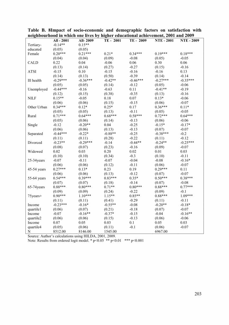
203
Table B. 8Impact of socio-economic and demographic factors on satisfaction with neighbourhood in which one lives by higher educational achievement, 2001 and 2009 All - 2001 All- 2009 TE - 2001 TE - 2009 NTE - 2001 NTE - 2009 Tertiary-educated
-0.14** 0.15** (0.05) (0.05) Female 0.20*** 0.21*** 0.21* 0.34*** 0.19*** 0.18*** (0.04) (0.04) (0.09) -0.08 (0.05) -0.05 CALD 0.22 0.04 -0.06 0.06 0.30 0.06 (0.13) (0.14) (0.27) -0.27 (0.15) -0.16 ATSI -0.15 0.10 -0.15 -0.16 -0.16 0.13 (0.14) (0.13) (0.50) -0.39 (0.14) -0.14 Ill health -0.29*** -0.36*** -0.42** -0.46*** -0.27*** -0.35*** (0.05) (0.05) (0.14) -0.12 (0.05) -0.06 Unemployed -0.44*** -0.16 -0.63 0.11 -0.41** -0.19 (0.12) (0.15) (0.38) -0.35 (0.13) -0.16 NILF 0.15** -0.05 0.18 0.07 0.13* -0.06 (0.06) (0.06) (0.15) -0.15 (0.06) -0.07 Other Urban 0.34*** 0.12* 0.25* 0.17 0.36*** 0.11* (0.05) (0.05) (0.13) -0.11 (0.05) -0.05 Rural 0.71*** 0.64*** 0.68*** 0.58*** 0.72*** 0.64*** (0.05) (0.06) (0.14) -0.13 (0.06) -0.06 Single -0.12 -0.20** 0.04 -0.25 -0.15* -0.17* (0.06) (0.06) (0.13) -0.13 (0.07) -0.07 Separated -0.44*** -0.22* -0.88** -0.25 -0.38*** -0.2 (0.11) (0.11) (0.28) -0.22 (0.11) -0.12 Divorced -0.23** -0.29*** -0.14 -0.44** -0.24** -0.25*** (0.08) (0.07) (0.23) -0.16 (0.09) -0.07 Widowed 0.02 0.03 0.20 0.02 0.01 0.03 (0.10) (0.10) (0.34) -0.3 (0.10) -0.11 25-34years -0.07 -0.11 -0.07 -0.04 -0.08 -0.16* (0.06) (0.06) (0.12) -0.11 (0.06) -0.07 45-54 years 0.27*** 0.13* 0.23 0.19 0.29*** 0.11 (0.06) (0.06) (0.13) -0.12 (0.07) -0.07 55-64 years 0.54*** 0.39*** 0.83*** 0.35* 0.50*** 0.38*** (0.07) (0.07) (0.18) -0.14 (0.07) -0.08 65-74years 0.88*** 0.80*** 0.71** 0.80*** 0.88*** 0.77*** (0.09) (0.09) (0.24) -0.22 (0.09) -0.1 75years+ 0.90*** 1.10*** 1.15** 0.85** 0.88*** 1.09*** (0.11) (0.11) (0.41) -0.29 (0.11) -0.11 Income quartile1
-0.23*** -0.16* -0.55** -0.08 -0.20** -0.18* (0.06) (0.07) (0.21) -0.18 (0.07) -0.07
Income quartile2
-0.07 -0.16** -0.37* -0.15 -0.04 -0.16** (0.06) (0.06) (0.15) -0.13 (0.06) -0.06
Income quartile4
0.07 0.05 0.03 0.1 0.05 0.03 (0.05) (0.06) (0.11) -0.1 (0.06) -0.07
N 8512.00 8146.00 1545.00 6967.00 Source: Author’s calculations using HILDA, 2001, 2009. Note: Results from ordered logit model. * p<0.05 ** p<0.01 *** p<0.001

204
Table B. 9Impact of socio-economic and demographic factors on satisfaction with local community by higher educational achievement, 2001 and 2009 All - 2001 All- 2009 TE - 2001 TE - 2009 NTE - 2001 NTE - 2009 Tertiary-educated
0.09 0.20*** (0.05) (0.05) Female 0.18*** 0.18*** 0.20* 0.42*** 0.18*** 0.12* (0.04) (0.04) (0.09) -0.08 (0.04) -0.05 CALD 0.24 0.05 0.23 -0.05 0.26 0.13 (0.13) (0.13) (0.27) -0.26 (0.15) -0.16 ATSI 0.13 0.33* -0.09 0.32 0.14 0.33* (0.14) (0.13) (0.47) -0.35 (0.15) -0.14 Ill health -0.30*** -0.29*** -0.21 -0.28* -0.30*** -0.29*** (0.05) (0.05) (0.13) -0.12 (0.05) -0.06 Unemployed -0.55*** -0.27* -0.73* -0.37 -0.52*** -0.25 (0.12) (0.14) (0.37) -0.31 (0.13) -0.15 NILF -0.05 -0.09 0.03 0.23 -0.06 -0.14* (0.06) (0.06) (0.15) -0.14 (0.06) -0.07 Other Urban 0.49*** 0.27*** 0.60*** 0.34** 0.48*** 0.25*** (0.05) (0.05) (0.13) -0.11 (0.05) -0.05 Rural 0.78*** 0.51*** 0.68*** 0.49*** 0.78*** 0.50*** (0.05) (0.06) (0.14) -0.13 (0.06) -0.06 Single -0.21*** -0.41*** -0.20 -0.69*** -0.21** -0.34*** (0.06) (0.06) (0.13) -0.12 (0.07) -0.07 Separated -0.60*** -0.28** -0.76** -0.2 -0.58*** -0.29* (0.11) (0.11) (0.28) -0.22 (0.12) -0.12 Divorced -0.28*** -0.39*** -0.07 -0.44** -0.30*** -0.38*** (0.08) (0.07) (0.22) -0.15 (0.09) -0.07 Widowed 0.06 -0.21* -0.29 -0.27 0.08 -0.17 (0.10) (0.10) (0.37) -0.31 (0.10) -0.1 25-34years -0.28*** -0.17** -0.41*** -0.14 -0.26*** -0.19** (0.05) (0.06) (0.12) -0.11 (0.06) -0.07 45-54 years 0.16** 0.16** 0.12 0.1 0.17** 0.19** (0.06) (0.06) (0.13) -0.12 (0.06) -0.07 55-64 years 0.48*** 0.40*** 0.58** 0.35* 0.47*** 0.43*** (0.07) (0.07) (0.18) -0.14 (0.07) -0.08 65-74years 0.78*** 0.86*** 0.39 0.61** 0.81*** 0.89*** (0.08) (0.09) (0.25) -0.22 (0.09) -0.1 75years+ 0.85*** 1.01*** 1.04* 0.5 0.84*** 1.04*** (0.11) (0.11) (0.44) -0.31 (0.11) -0.11 Income quartile1
-0.08 -0.03 0.02 -0.14 -0.10 -0.03 (0.06) (0.07) (0.21) -0.18 (0.07) -0.07
Income quartile2
-0.10 -0.05 -0.16 0.08 -0.09 -0.07 (0.05) (0.06) (0.15) -0.13 (0.06) -0.06
Income quartile4
-0.10 -0.10 -0.07 -0.07 -0.12 -0.13 (0.05) (0.05) (0.11) -0.1 (0.06) -0.07
N 8512.00 8135.00 1545.00 6967.00 Source: Author’s calculations using HILDA, 2001, 2009. Note: Results from ordered logit model. * p<0.05 ** p<0.01 *** p<0.001

205
Table B. 10Impact of socio-economic and demographic factors on satisfaction with the partner by higher educational achievement, 2001 and 2009 Partner All - 2001 All- 2009 TE - 2001 TE - 2009 NTE - 2001 NTE - 2009 Tertiary-educated
-0.16** (0.05) Female -0.15*** -0.01 -0.08 -0.20*** -0.09* (0.04) (0.09) (-0.08) (0.05) -0.05 CALD 0.02 0.28 -0.2 -0.09 -0.54*** (0.14) (0.28) (-0.26) (0.16) -0.16 ATSI 0.11 1.13* -0.04 0.06 -0.29* (0.14) (0.53) (-0.4) (0.15) -0.13 Ill health -0.04 0.04 -0.18 -0.05 -0.17** (0.05) (0.14) (-0.12) (0.05) -0.05 Unemployed -0.14 -0.07 -0.43 -0.11 -0.2 (0.12) (0.41) -0.33 (0.13) -0.15 NILF 0.22*** 0.31* 0.07 0.22*** 0.06 (0.06) (0.16) -0.14 (0.06) -0.06 Other Urban 0.15** 0.04 0.15 0.17** 0.09 (0.05) (0.13) -0.11 (0.05) -0.05 Rural 0.11 -0.05 0.03 0.13* 0.04 (0.05) (0.14) -0.13 (0.06) -0.06 Single -3.55*** -3.32*** -2.72*** -3.66*** -2.46*** (0.08) (0.16) -0.14 (0.09) -0.08 Separated -3.34*** -3.28*** -2.39*** -3.35*** -2.22*** (0.11) (0.29) -0.22 (0.12) -0.12 Divorced -3.56*** -3.66*** -1.85*** -3.54*** -1.70*** (0.10) (0.25) -0.16 (0.10) -0.08 Widowed -4.41*** -4.08*** -2.70*** -4.39*** -2.84*** (0.11) (0.36) -0.28 (0.12) -0.1 25-34years 0.29*** 0.31* 0.41*** 0.29*** 0.09 (0.06) (0.12) -0.11 (0.06) -0.07 45-54 years 0.24*** -0.09 0.16 0.32*** 0.05 (0.06) (0.13) -0.12 (0.07) -0.07 55-64 years 0.43*** 0.44* 0.39** 0.43*** 0.36*** (0.07) (0.17) -0.14 (0.08) -0.07 65-74years 0.59*** 0.12 0.36 0.63*** 0.64*** (0.09) (0.24) -0.2 (0.09) -0.09 75years+ 0.39*** 0.64 0.09 0.38** 0.43*** (0.11) (0.42) -0.29 (0.12) -0.11 Income quartile1
-0.18** -0.35 -0.05 -0.18* -0.24*** (0.07) (0.20) -0.18 (0.07) -0.07
Income quartile2
-0.12* -0.14 0.21 -0.12* -0.09 (0.06) (0.15) -0.12 (0.06) -0.06
Income quartile4
-0.06 0.06 0.32*** -0.10 0.06 (0.06) (0.11) -0.1 (0.07) -0.07
N 8512.00 1545.00 6967.00 Source: Author’s calculations using HILDA, 2001, 2009. Note: Results from ordered logit model. * p<0.05 ** p<0.01 *** p<0.001
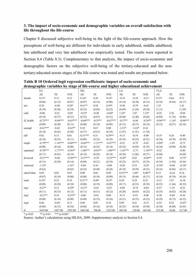
206
3. The impact of socio-economic and demographic variables on overall satisfaction with life throughout the life-course
Chapter 8 discussed subjective well-being in the light of the life-course approach. How the
perceptions of well-being are different for individuals in early adulthood, middle adulthood,
late adulthood and very late adulthood was empirically tested. The results were reported in
Section 8.4 (Table 8.3). Complementary to that analysis, the impact of socio-economic and
demographic factors on the subjective well-being of the tertiary-educated and the non-
tertiary-educated across stages of the life course was tested and results are presented below.
Table B 10 Ordered logit regression coefficients: impact of socio-economic and demographic variables by stage of life-course and higher educational achievement
EA
MA
LA
VLA
All TE NTE All TE NTE All TE NTE All TE NTE female 0.13* 0.12 0.12 0.16* 0.26 0.16* -0.18 -0.28 -0.21 0.32* 0.66 0.31
(0.06) (0.12) (0.07) (0.07) (0.14) (0.08) (0.14) (0.38) (0.15) (0.16) (0.64) (0.17)
atsi 0.29 -0.48 0.38* 0.61** 0.54 0.59* -0.50 -0.79 -0.41 1.35
1.41
(0.19) (0.58) (0.19) (0.23) (0.69) (0.25) (0.49) (1.64) (0.54) (1.31)
(1.29)
cald -0.06 -0.21 -0.05 -0.53* -0.20 -0.68* 1.22* 1.07 1.32* -0.22 2.56 -0.84
(0.18) (0.37) (0.21) (0.25) (0.47) (0.31) (0.60) (2.40) (0.64) (0.84) (1.76) (0.96)
ill_health -0.72*** -0.94*** -0.65*** -0.64*** -0.53** -0.67*** -0.37** -0.44 -0.38** -0.94*** -1.16* -0.94***
(0.09) (0.20) (0.11) (0.08) (0.19) (0.09) (0.13) (0.37) (0.14) (0.15) (0.57) (0.16)
unempl -0.61*** -0.42 -0.62** 0.10 0.67 0.00 -2.33* -3.62* 0.34
(0.18) (0.42) (0.20) (0.27) (0.67) (0.29) (1.07) (1.41) (1.54)
nilf 0.02 0.13 0.01 0.31*** 0.31 0.29** -0.13 -0.19 -0.09 -0.19 0.26 -0.40
(0.10) (0.23) (0.11) (0.09) (0.23) (0.10) (0.19) (0.52) (0.21) (0.34) (0.78) (0.39)
single -0.79*** -1.16*** -0.68*** -0.68*** -1.31*** -0.47*** -0.52 -0.79 -0.42 -0.84* -1.83 -0.73
(0.08) (0.16) (0.09) (0.12) (0.25) (0.14) (0.32) (0.85) (0.35) (0.34) (0.99) (0.38)
separated -0.78*** -1.77*** -0.56** -1.04*** -0.93** -1.09*** -1.43*** -2.73 -1.36*** -0.32
-0.40
(0.17) (0.41) (0.19) (0.15) (0.29) (0.18) (0.36) (1.86) (0.37) (0.68)
(0.68)
divorced -0.51*** -0.46 -0.50*** -0.37*** -0.39 -0.35*** -0.45* 0.83 -0.68** -0.59 0.08 -0.75*
(0.13) (0.30) (0.14) (0.09) (0.21) (0.10) (0.22) (0.57) (0.25) (0.34) (1.02) (0.36)
widowed -1.53*
-1.41* -0.04 0.10 -0.08 -0.20 0.53 -0.29 -0.34* -0.49 -0.34*
(0.62)
(0.62) (0.22) (0.49) (0.24) (0.19) (0.59) (0.21) (0.16) (0.66) (0.17)
otherUrban 0.05 0.03 0.07 0.09 0.05 0.09 0.53*** 1.04* 0.48** 0.15 -0.34 0.16
(0.07) (0.16) (0.08) (0.08) (0.18) (0.09) (0.15) (0.44) (0.17) (0.16) (0.74) (0.16)
rural 0.19* 0.25 0.19 0.27** 0.49* 0.23* 0.24 0.25 0.25 -0.12 1.87 -0.18
(0.09) (0.20) (0.10) (0.08) (0.19) (0.09) (0.17) (0.51) (0.18) (0.22) (1.46) (0.23)
inq1 -0.27* 0.13 -0.29* -0.27* -0.41 -0.23 -0.05 -0.74 -0.04 -0.37 -1.35 -0.32
(0.11) (0.33) (0.12) (0.11) (0.31) (0.12) (0.20) (0.65) (0.22) (0.25) (0.82) (0.28)
inq2 -0.21** 0.10 -0.25** -0.06 -0.41 0.00 -0.15 -0.91 -0.06 -0.38 -0.69 -0.36
(0.08) (0.18) (0.09) (0.09) (0.23) (0.10) (0.21) (0.53) (0.23) (0.29) (0.73) (0.32)
inq4 0.06 -0.04 0.13 0.09 0.05 0.10 0.09 0.41 -0.15 -0.55 0.52 -0.85*
(0.08) (0.13) (0.10) (0.08) (0.16) (0.10) (0.25) (0.54) (0.30) (0.38) (0.88) (0.43)
N 3619.00 1027.00 2592.00 3063.00 708.00 2355.00 803.00 120.00 683.00 675.00 58.00 617.00 * p<0.05 ** p<0.01 *** p<0.001"
Source: Author’s calculations using HILDA, 2009. Supplementary analysis to Section 8.4.

207
Appendix C. Technical appendix
This technical appendix addresses two of the biases identified in quality of life research, and
previously discussed in Section 4.5. Six methodological biases have been identified at that
time: the age group bias, cohort bias, centrality of life-domains over the life-course (or
focussing effect, Plagnol 2010), instrumentation biases, differences between subjective and
objective levels of well-being, potential differences between SWB assessed as satisfaction
and SWB assessed as happiness. Section 4.5 discussed how the analysis attends to these
biases, and directed the reader towards the section of the thesis in which each bias was
addressed. This appendix discusses the instrumentation bias and the difference in levels of
SWB when measured as satisfaction or happiness.

208
1. Instrumentation or participation bias
Following work by Baltes (1968), Bell (1953), Schaie (1965) and Windle (1954), Baird et al.
(2010) investigated whether “the simple act of answering the same question on multiple
occasions might lead people to change their responses over time” (p. 186, also discussed by
Choquette and Hesselbrock, 1987 and Sharpe and Gilbert, 1998). They suggest the use of
refreshment samples to isolate the effect sought in the investigation from noise like historical
events or participation biases.
HILDA provides data for a repeated cohort of individuals (n=7,721) for longitudinal
analysis, as well as for refreshed samples of individuals (19,914 respondents in 2001, 13,301
in 2009 etc.). Individuals that were not in all waves of interviews are considered to make the
‘refreshed’ sample and their levels of satisfaction are compared to the satisfaction levels of
the 7,721 repeated respondents in 2009. If the two groups have similar levels of satisfaction
then it can be concluded that there are no differences between the two groups and there is no
participation bias reflected in the self-assessment of well-being. However, remaining in the
survey may be indicative of some intrinsic characteristics (such as commitment) and the
differences may in fact be present since the beginning of the survey.
The same exercise is conducted for 2001 data. Furthermore, given the purpose of this
study – to map differences between tertiary education graduates and the rest of the
population, the 2001 and 2009 differences between the repeated and refreshed samples of TE
and NTE are as well graphed (Fig.C.1 and Fig.C.2 respectively). While there is a an observed
trend of slightly higher levels of satisfaction in 2009 for the cohort that participated in all
waves of HILDA (marked through the darker columns in Fig.10), satisfaction with the feeling
of safety and satisfaction with health are lower for this repeated sample.
The highest and most obvious differences occur in terms of satisfaction with the
financial situation, feeling part of the local community and satisfaction with health (a
difference between repeated and fresh respondents in 2009 of about 0.3 points or more).
Given the low or no oscillations in self-assessed wellbeing (Cummins, 2010), such
differences may be considered well high.
It can then be concluded that, although for most domains (satisfaction with their
home, satisfaction with employment opportunities, with safety, neighbourhood, or
satisfaction with life as a whole), there are no major differences between the repeated sample
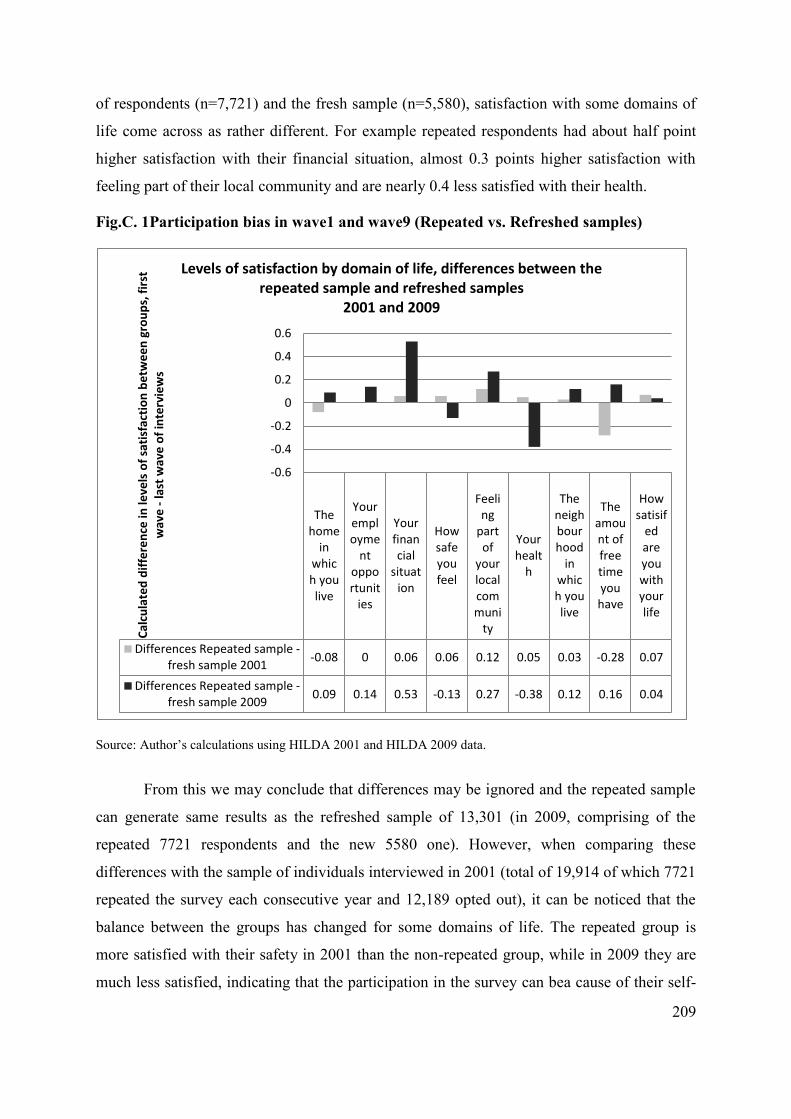
209
of respondents (n=7,721) and the fresh sample (n=5,580), satisfaction with some domains of
life come across as rather different. For example repeated respondents had about half point
higher satisfaction with their financial situation, almost 0.3 points higher satisfaction with
feeling part of their local community and are nearly 0.4 less satisfied with their health.
Fig.C. 1Participation bias in wave1 and wave9 (Repeated vs. Refreshed samples)
Source: Author’s calculations using HILDA 2001 and HILDA 2009 data.
From this we may conclude that differences may be ignored and the repeated sample
can generate same results as the refreshed sample of 13,301 (in 2009, comprising of the
repeated 7721 respondents and the new 5580 one). However, when comparing these
differences with the sample of individuals interviewed in 2001 (total of 19,914 of which 7721
repeated the survey each consecutive year and 12,189 opted out), it can be noticed that the
balance between the groups has changed for some domains of life. The repeated group is
more satisfied with their safety in 2001 than the non-repeated group, while in 2009 they are
much less satisfied, indicating that the participation in the survey can bea cause of their self-
Thehome
inwhich youlive
Youremployme
ntopportunit
ies
Yourfinancial
situation
Howsafeyoufeel
Feeling
partof
yourlocalcommuni
ty
Yourhealt
h
Theneighbourhood
inwhich youlive
Theamount offreetimeyouhave
Howsatisif
edareyouwithyourlife
Differences Repeated sample -fresh sample 2001
-0.08 0 0.06 0.06 0.12 0.05 0.03 -0.28 0.07
Differences Repeated sample -fresh sample 2009
0.09 0.14 0.53 -0.13 0.27 -0.38 0.12 0.16 0.04
-0.6
-0.4
-0.2
0
0.2
0.4
0.6
Cal
cula
ted
dif
fere
nce
in le
vels
of
sati
sfac
tio
n b
etw
ee
n g
rou
ps,
fir
st
wav
e -
last
wav
e o
f in
terv
iew
s
Levels of satisfaction by domain of life, differences between the repeated sample and refreshed samples
2001 and 2009

210
appreciation of safety to decline. Similarly, they are less satisfied with their health in 2009,
while in 2001 they are more satisfied that the rest of the population. The differences depicted
in Fig.C.2 indicate that a participation bias may be present in HILDA in terms of self-
assessed satisfaction with various domains of life (although not much overall satisfaction
with life). For this reason the refreshed samples are preferred for the analysis.
A similar comparison between the differences of satisfaction of repeated and fresh
participants in 2009 and 2001 respectively is separately conducted for individuals with higher
qualifications (TE) and the rest of the population (NTE). While the direction of the bias is
similar to that of the general population for the two groups, the intensity is greater for NTE.
For example, if they participate in all waves of the survey, NTE have greater levels of
satisfaction with their financial situation, feeling part of their local community and their free
time, but are also much less satisfied with their health than they were at the beginning of the
survey (2001) and the TE in 2009 (Fig.C.2 and Fig.C.3). These findings are again indicative
that, in particular for this thesis that investigates differences in SWB by highest education
level achieved, it is important to account for the participation bias (Baird et al., 2010) and use
refreshed samples even in multiple-year analysis.

211
Fig.C. 2Participation bias in wave1 and wave9 (Repeated vs. Refreshed samples), TE
Source: Author’s calculations using HILDA 2001 and HILDA 2009 data.
Thehome
inwhich
youlive
Youremployme
ntopportuniti
es
Yourfinanc
ialsituat
ion
Howsafeyoufeel
Feeling part
ofyourlocalcom
munity
Yourhealt
h
Theneighbourhoodin
whichyoulive
Theamount offreetimeyouhave
Howsatisif
edareyouwithyourlife
Differences Repeated sample -fresh sample 2001
0.13 0.13 0.1 0.09 0.12 -0.01 -0.06 -0.27 0.13
Differences Repeated sample -fresh sample 2009
0 0.13 0.29 0 0.41 -0.13 0.09 -0.01 0.1
-0.4-0.3-0.2-0.1
1E-150.10.20.30.40.50.6
Cal
cula
ted
dif
fere
nce
in le
vels
of
sati
sfac
tio
n b
etw
ee
n
gro
up
s, f
irst
wav
e t
o la
st w
ave
of
inte
rvie
ws
Differences between the repeated sample and fresh sample 2001 and 2009, HQs

212
Fig.C. 3Participation bias in wave1 and wave9 (Repeated vs. Refreshed samples), NTE
Source: Author’s calculations using HILDA 2001 and HILDA 2009 data.
Thehome
inwhich
youlive
Youremployme
ntopportuniti
es
Yourfinanc
ialsituat
ion
Howsafeyoufeel
Feeling part
ofyourlocalcom
munity
Yourhealt
h
Theneighbourhoodin
whichyoulive
Theamount offreetimeyouhave
Howsatisif
edareyouwithyourlife
Differences Repeated sample -fresh sample 2001
-0.1 -0.09 0.01 0.05 0.12 0.05 0.05 -0.22 0.06
Differences Repeated sample -fresh sample 2009
0.12 0.07 0.55 -0.17 0.23 -0.45 0.12 0.24 0.03
-0.5
-0.4
-0.3
-0.2
-0.1
0
0.1
0.2
0.3
0.4
0.5
0.6
Cal
cula
ted
dif
fere
nce
in le
vels
of
sati
sfac
tio
n b
etw
ee
n g
rou
ps,
fir
st
wav
e t
o la
st w
ave
of
inte
rvie
ws
Differences between the repeated sample and refreshed sample 2001 and 2009, non-HQs

213
2. Satisfaction with life and happiness or cognitive and affective measures of wellbeing
Table C. 1 Happiness with life overall, AuSSA 2009 (%) Tertiary-educated Not Tertiary-educated Total Very happy 35.8 31.7 32.5 Fairly happy 58.2 56.7 57.0 Not very happy 4.8 8.8 8.1 Not at all happy 0.7 1.8 1.6 Can’t choose 0.4 0.9 0.8 Total 100 100 100 N 2305 861 3166 Note: Pearson Chi-Square <.005. Source: Author’s calculation using AuSSA 2009. Sampling weight was used for cross tabulation; total N is reported from un-weighted sample.
Table C. 2 Satisfaction with life overall, HILDA 2009 (%) Tertiary-educated Not tertiary-educated Total Totally satisfied 5.7 11.5 10.1 9 23.1 20.7 21.3 8 36.7 33.5 34.3 7 23.8 18.8 20.0 6 6.5 7.0 6.8 Neither satisfied nor dissatisfied
2.5 5.3 4.6
4 0.8 1.2 1.1 3 0.5 0.9 0.8 2 0.1 0.7 0.5 1 0.3 0.5 0.4 Totally dissatisfied 0.0 0.1 0.1 Total 100 100 100 N 2645 8030 10675 Note: Pearson’s Chi-Square <.005. Source: Author’s calculations using HILDA, 2009. Sampling weight was used for cross tabulation; total N is reported from un-weighted sample.
Table C. 3 Mean levels of SWB by higher educational achievement using four distinct measures SWB measured as Tertiary-educated Non-tertiary-educated Overall satisfaction 7.82 7.78 Average satisfaction 7.37 7.15 Happiness1 Personal Well-Being Index2 7.49 1. Happiness as measured in AuSSA 2009. 2. Disaggregated mean value of the PWI by tertiary educational achievement was not available; the reported value is the overall population mean.

214
3. SWB by degree level or highest school level
Table C. 4 Overall satisfaction and average satisfaction by higher educational level achieved Derived satisfaction from eight domains (average satisfaction)
History: Highest education level achieved N Median Mean
Std. Deviation
Postgrad - masters or doctorate 477 7.375 7.2851 1.07984 Grad diploma, grad certificate 652 7.5 7.3867 1.13204 Bachelor or honours 1516 7.375 7.2251 1.13395 Adv diploma, diploma 1048 7.125 7.044 1.28342 Cert III or IV 2365 7.125 6.9569 1.28845 Cert I or II 167 6.75 6.6774 1.45576 Cert not defined 61 6.75 6.6598 1.43435 Year 12 1227 7 6.9439 1.35978 Year 11 and below 3155 6.875 6.8003 1.38732 Undetermined 7 6.875 6.8393 1.36495 Total 10675 7.125 6.9905 1.30518
How satisfied are you with your life? (overall satisfaction)
History: Highest education level achieved N Median Mean
Std. Deviation
Postgrad - masters or doctorate 477 8 7.78 1.287 Grad diploma, grad certificate 652 8 7.92 1.244 Bachelor or honours 1515 8 7.85 1.246 Adv diploma, diploma 1046 8 7.83 1.349 Cert III or IV 2361 8 7.78 1.456 Cert I or II 167 8 7.77 1.725 Cert not defined 61 8 7.67 1.661 Year 12 1225 8 7.79 1.446 Year 11 and below 3146 8 7.91 1.648 Undetermined 7 8 6.71 2.69 Total 10657 8 7.84 1.466
Source: Author’s calculations using HILDA, 2009.