The overdue Copernican Revolution in Economics

Steve KeenKingston University London

IDEAeconomicsMinsky Open Source System Dynamics

www.debtdeflation.com/blogs

What does Economics have in common with Ptolemy?

• (1) The propensity to start from “a priori” beliefs rather than research

• (2) A plausible but false model of reality• Ptolemy’s starting point: Aristotle’s vision of the universe…

– “the heavens were literally composed of 55 concentric, crystalline spheres to which the celestial objects were attached and which rotated at different velocities with the Earth at the center”

• Ptolemy’s puzzle: how to reconcile this vision with the observable behaviour of the planets (“wanderers” in Greek)?

• Answer: epicycles—spheres on spheres

• Literally any actual path can be described using epicycle

• So the model was plausible—but wrong

What does Economics have in common with Ptolemy?

• Ditto economics on many topics—but especially money

• Economics’ starting point: Adam Smith & “The propensity to truck & barter…”• “THIS division of labour, from which so many advantages are derived, is …the necessary …consequence of a certain propensity in human nature …

• the propensity to truck, barter, and exchange one thing for another…

• It is common to all men, and to be found in no other race of animals, which seem to know neither this nor any other species of contracts…

• Nobody ever saw a dog make a fair and deliberate exchange of one bone for another with another dog…”

• Origin of Neoclassical vision of money as “veil over barter”

• Ensconsed in mainstream macroeconomics– Banks, debt and money play no essential

role…

What does Economics have in common with Ptolemy?

• What brought Ptolemaic astronomy to an end?– More realistic (but incomplete!), simpler observation-

based theory– Anomalies: moons orbiting Jupiter, craters on the Moon– Accurate predictions of extended Copernicus model

• Elliptic motion replaces circular, epicycles eliminated• Newton’s theory of gravity

– Accurate prediction of Halley’s comet• What could have brought Neoclassical economics to an

end?– The global financial crisis of 2007

• Not merely failure to predict an event• But a complete anomaly in their equilibrium, non-

monetary vision of the economy• Here economics differs from astronomy

– Laymen thought astronomers were experts on “the heavens”: True

– Laymen think economists are experts on money: False!

The conventional “veil over barter” vision of money

• Mainstream economics generally ignores banks, debt & money– “self-proclaimed true Minskyites view banks as

institutions that are somehow outside the rules that apply to the rest of the economy, as having unique powers for good and/or evil.

– I guess I don't see it that way.– As I (and I think many other economists) see it, …Banks

don't create demand out of thin air any more than anyone does by choosing to spend more; and banks are just one channel linking lenders to borrowers.

– I know I'll get the usual barrage of claims that I don't understand banking; actually, I think I do, and it's the mystics who have it wrong.” (Krugman 2012, “Banking Mysticism”)

• If Krugman’s model of banking were accurate, debt would have “no significant macroeconomic effects” (except during a liquidity trap)

The conventional “veil over barter” vision of money

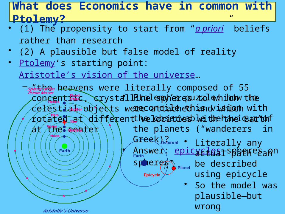
• “Think of it this way: when debt is rising, it’s not the economy as a whole borrowing more money.

• It is, rather, a case of less patient people—people who for whatever reason want to spend sooner rather than later—borrowing from more patient people.” (Krugman 2012, pp. 146-47)

• “The idea of debt-deflation goes back to Irving Fisher… Fisher's idea was less influential in academic circles, though, because of the counterargument that debt-deflation represented no more than a re-distribution from one group (debtors) to another (creditors).

• Absent implausibly large differences in marginal spending propensities among the groups, it was suggested, pure redistributions should have no significant macroeconomic effects.” (Bernanke 200, p. 24)

• Let’s check this out:• Modeling Eggertsson & Krugman’s 2012 model in Minsky…

– a system dynamics program tailored for monetary modeling

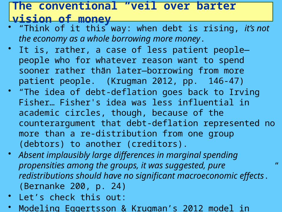
System dynamics• Graphical method of building dynamic models

– Invented in 1950s– “Bread & butter” in engineering & manufacturing

process control• Matlab’s Simulink (retail price about US$20,000),

Vissim…– Commonplace in sociology

• Vensim, Stella…• Build equations using a flowchart…

• Program builds equations in the background…Output 0

Productivity 0

OutputEmployment

Productivity

• Overkill for simple equations, essential for complex dynamic systems…

System dynamics• Dynamics—systems with rates of change

• Integrals used for technical reasons…• Model now an “Ordinary Differential Equation”

ratio

ratio

CO 3

Productivity 1

Investment 30

CapitalOutput

CO

OutputEmployment

Productivity

Capital(0) 300

CapitalInvestment

d

dt

• “Ordinary”: involves time but not location• “Differential”: rate of change modelled– Dynamics & change– Not “statics” & equilibrium• Models get interesting with more

“system states” (variables) & nonlinearity

• Minsky adds ability to model money flows using accounting “double entry bookkeeping”…

System dynamics for monetary flows• Flowchart paradigm works really well for physical flows

– Petrol in tank flowing into cylinder…– One direction only

• Difficult to impossible for financial flows– Every transaction has two “directions”

• Out of one account, into another• Operation has to have opposite signs

– Easy to forget in flowchart, get signs wrong• Solution: borrow idea from accountants

– Double-entry bookkeeping– Record every transaction on one row

• Two entities (buyer and seller) recorded on one row– Every row “sums to zero”– For example, a simple “Buy and Sell” between two

agents…

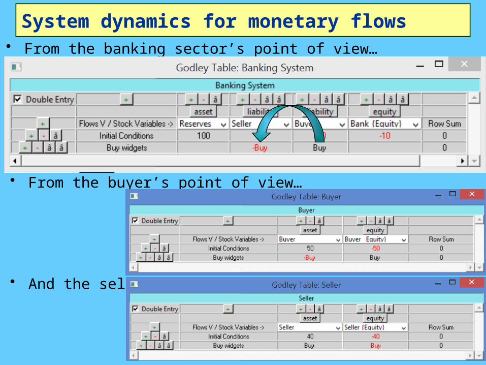
System dynamics for monetary flows• From the banking sector’s point of view…

• From the buyer’s point of view…

• And the seller’s

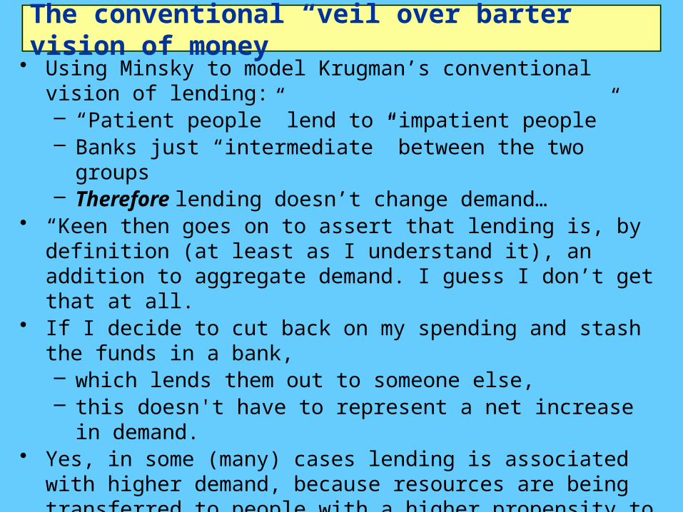
The conventional “veil over barter” vision of money

• Using Minsky to model Krugman’s conventional vision of lending:– “Patient people” lend to “impatient people”– Banks just “intermediate” between the two groups– Therefore lending doesn’t change demand…

• “Keen then goes on to assert that lending is, by definition (at least as I understand it), an addition to aggregate demand. I guess I don’t get that at all.

• If I decide to cut back on my spending and stash the funds in a bank,– which lends them out to someone else,– this doesn't have to represent a net increase in demand.

• Yes, in some (many) cases lending is associated with higher demand, because resources are being transferred to people with a higher propensity to spend;

• but Keen seems to be saying something else, and I'm not sure what.

• I think it has something to do with the notion that creating money = creating demand, but again that isn’t right in any model I understand.”

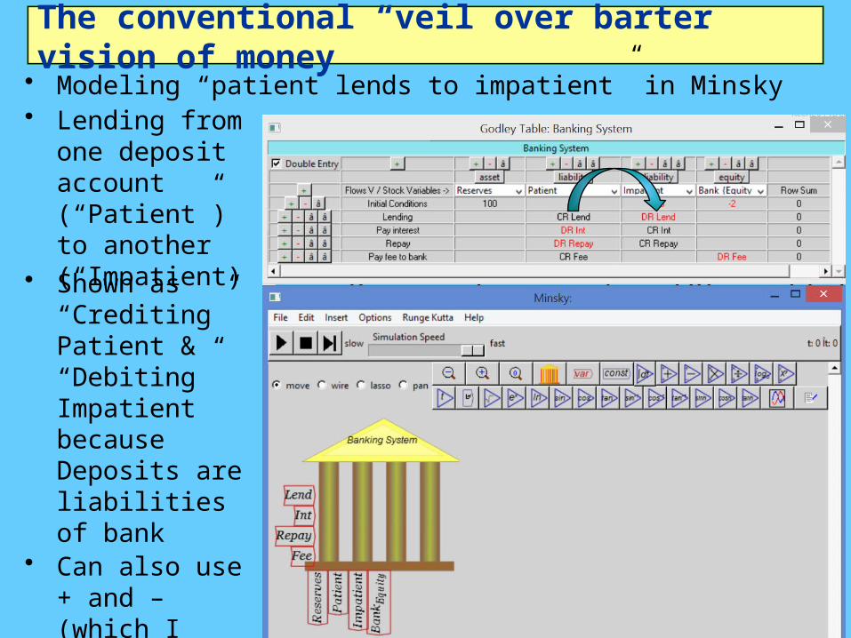
The conventional “veil over barter” vision of money

• Modeling “patient lends to impatient” in Minsky• Lending from

one deposit account (“Patient”) to another (“Impatient)• Shown as “Crediting” Patient & “Debiting” Impatient because Deposits are liabilities of bank

• Can also use + and – (which I prefer)

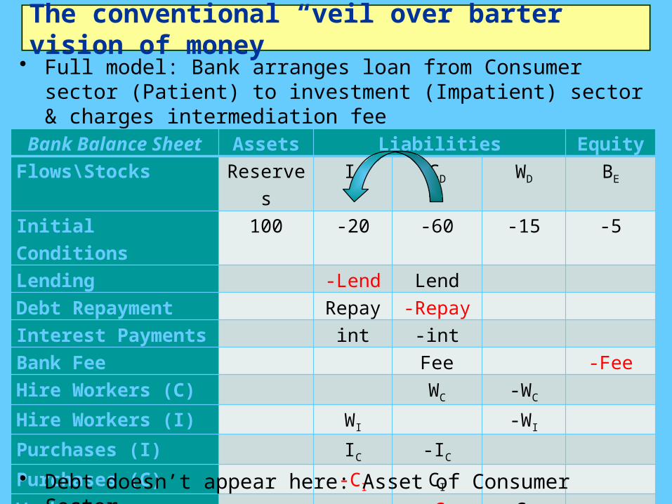
The conventional “veil over barter” vision of money

• Full model: Bank arranges loan from Consumer sector (Patient) to investment (Impatient) sector & charges intermediation fee

• Workers hired, output produced & sold, investment… Bank Balance Sheet

Assets Liabilities Equity

Flows\Stocks Reserves ID CD WD BE

Initial Conditions 100 -20 -60 -15 -5Lending   -Lend Lend    Debt Repayment   Repay -Repay    Interest Payments   int -int    Bank Fee     Fee   -FeeHire Workers (C)     WC -WC  Hire Workers (I)   WI   -WI  Purchases (I)   IC -IC    Purchases (C)   -CI CI    Workers Consumption

    -CW CW  

Bankers Consumption

    -CB   CB

Bankers Investment

  -IB     IB

• Debt doesn’t appear here: Asset of Consumer Sector…

The conventional “veil over barter” vision of money

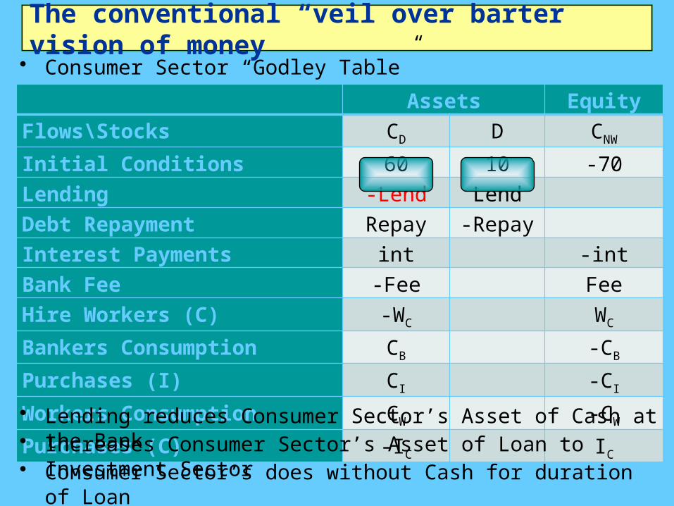
• Consumer Sector “Godley Table”

  Assets EquityFlows\Stocks CD D CNW

Initial Conditions 60 10 -70Lending -Lend Lend  Debt Repayment Repay -Repay  Interest Payments int   -intBank Fee -Fee   FeeHire Workers (C) -WC   WC

Bankers Consumption CB   -CB

Purchases (I) CI   -CI

Workers Consumption CW   -CW

Purchases (C) -IC   IC• Lending reduces Consumer Sector’s Asset of Cash at the Bank• Increases Consumer Sector’s Asset of Loan to Investment Sector• Consumer Sector’s does without Cash for duration of Loan

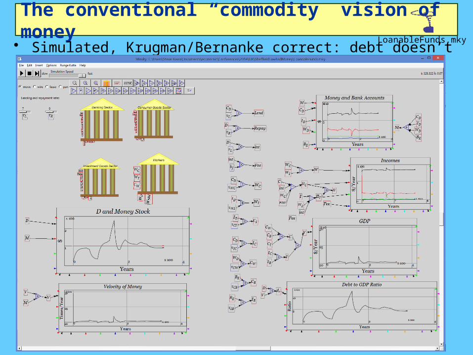
The conventional “commodity” vision of money

• Simulated, Krugman/Bernanke correct: debt doesn’t matter…

LoanableFunds.mky

The conventional “commodity” vision of money

• But a “Mystical” thought: what if banks are actually the lenders???

EndogenousMoney.mky

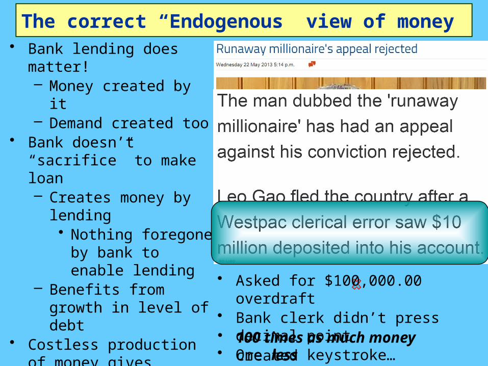
The correct “Endogenous” view of money

• Bank lending does matter!– Money created by it– Demand created too

• Bank doesn’t “sacrifice” to make loan– Creates money by

lending• Nothing foregone

by bank to enable lending

– Benefits from growth in level of debt

• Costless production of money gives incentive to over-produce– New Zealand petrol

station owner story…

• Asked for $100,000.00 overdraft• Bank clerk didn’t press decimal

point• One less keystroke…• 100 times as much money

created

Endogenous money & systemic crises• Smith’s “Truck & barter” vision of origins of money a myth.

– Money originated in credit (Graeber 2011; Martin 2013)– Demand-generating effect of bank lending causes

booms & busts…• Hyman Minsky on the unstable & monetary nature of

capitalism– “In this "Chicago" view there exists a financial system…

which would make serious financial disturbances impossible. It is the task of monetary analysis to design such a financial system, and of monetary policy to execute the design…

– The alternative polar view, which I call unreconstructed Keynesian, is that capitalism is inherently flawed, being prone to booms, crises, and depressions.

– This instability, in my view, is due to characteristics the financial system must possess if it is to be consistent with full-blown capitalism.

– Such a financial system will be capable of both generating signals that induce an accelerating desire to invest and of financing that accelerating investment.” (Minsky 1982, p. 279)

Minsky’s “Financial Instability Hypothesis”

• “The natural starting place for analyzing the relation between debt and income is to take an economy with a cyclical past that is now doing well…

• As the period over which the economy does well lengthens, two things become evident in board rooms. Existing debts are easily validated and units that were heavily in debt prospered; it paid to lever…

• Stable growth is inconsistent with the manner in which investment is determined in an economy in which debt-financed ownership of capital assets exists, and the extent to which such debt financing can be carried is market determined.

• It follows that the fundamental instability of a capitalist economy is upward.

• The tendency to transform doing well into a speculative investment boom is the basic instability in a capitalist economy. (Minsky 1982, pp. 66-67)

• My contribution: modelling Minsky by extending nonlinear cyclical but non-monetary Goodwin model

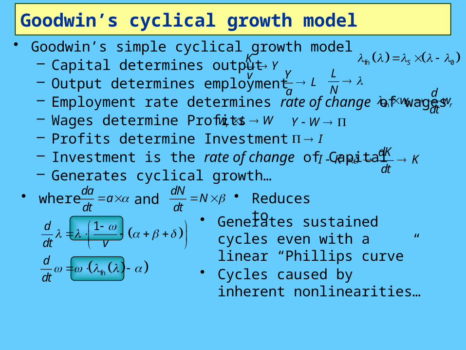
Goodwin’s cyclical growth model• Goodwin’s simple cyclical growth model

– Capital determines output– Output determines employment– Employment rate determines rate of change of wages– Wages determine Profits– Profits determine Investment– Investment is the rate of change of Capital– Generates cyclical growth…

KY

v

YL

a

L

N

fn 0S

fn r r

dw w

dt

rw L W Y W I

dKI K K

dt

• whereda

adt

anddN

Ndt

• Reduces to

fn

1d

dt v

d

dt

• Generates sustained cycles even with a linear “Phillips curve”

• Cycles caused by inherent nonlinearities…

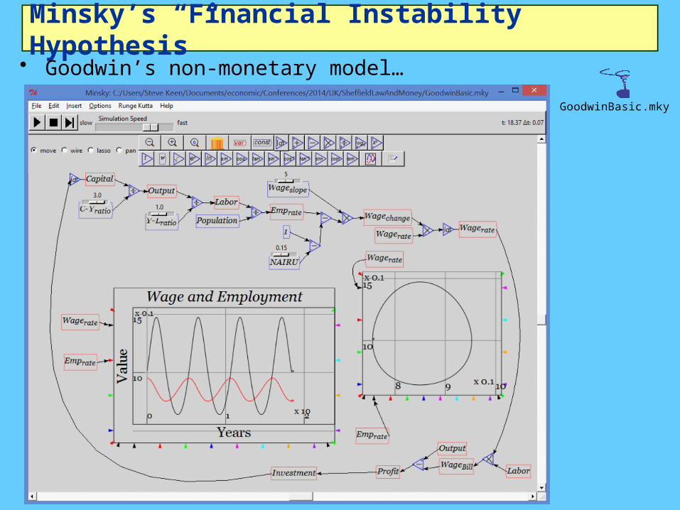
Minsky’s “Financial Instability Hypothesis”

• Goodwin’s non-monetary model…

GoodwinBasic.mky

Minsky’s “Financial Instability Hypothesis”

• Adding monetary realism…– Investment exceeds profits during boom– Investment less than profits during a slump– Difference financed by change in debt– Banks charge interest on debt…

• Endogenous money key here—debt financed spending boosts demand

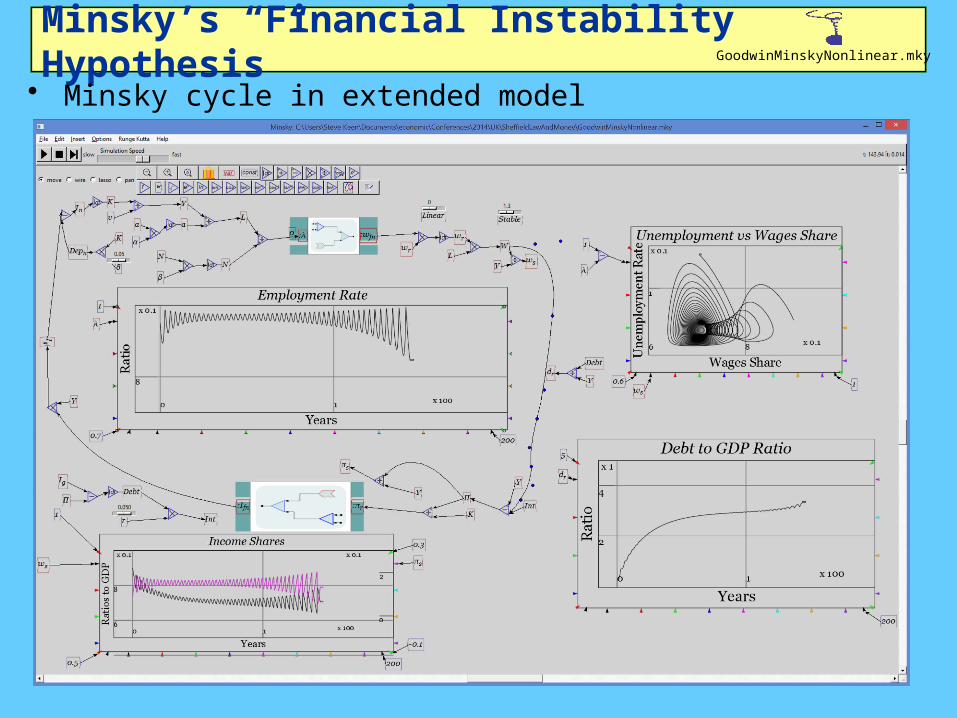
• Crucial features of extended model– Complexity: regular behaviour of base model replaced by

potential for complex behaviour• “Stability leads to instability”

– Rising debt to GDP ratio: instability– With rising ratio comes apparent “Great Moderation”

• Declining volatility in employment & inflation (proxy)– Then subsequent breakdown– Rising inequality with falling workers’ share of output

• Even though firms borrow, not workers…

Goodwin’s cyclical growth model• Empirically realistic with nonlinear Phillips curve

– Forthcoming paper by Grasselli• (Contra Harvie 2000—simple error in econometrics)• Average of cycle conforms to average of 8/10 OECD

countries• My Minsky extension

– (Nonlinear) Investment function based on rate of profit• Capitalists invest more than profits during boom• Less than profits during slump

– Linear function used here for simplicity– Investment minus profit gap financed by change in debt– Profit net of interest on debtnr

nY W r D

K K v

fn Sr EI fnI Y I n

dDI

dt

• Reduces to 3-dimensional system where “Period Three Implies Chaos” (Li and Yorke 1975)…

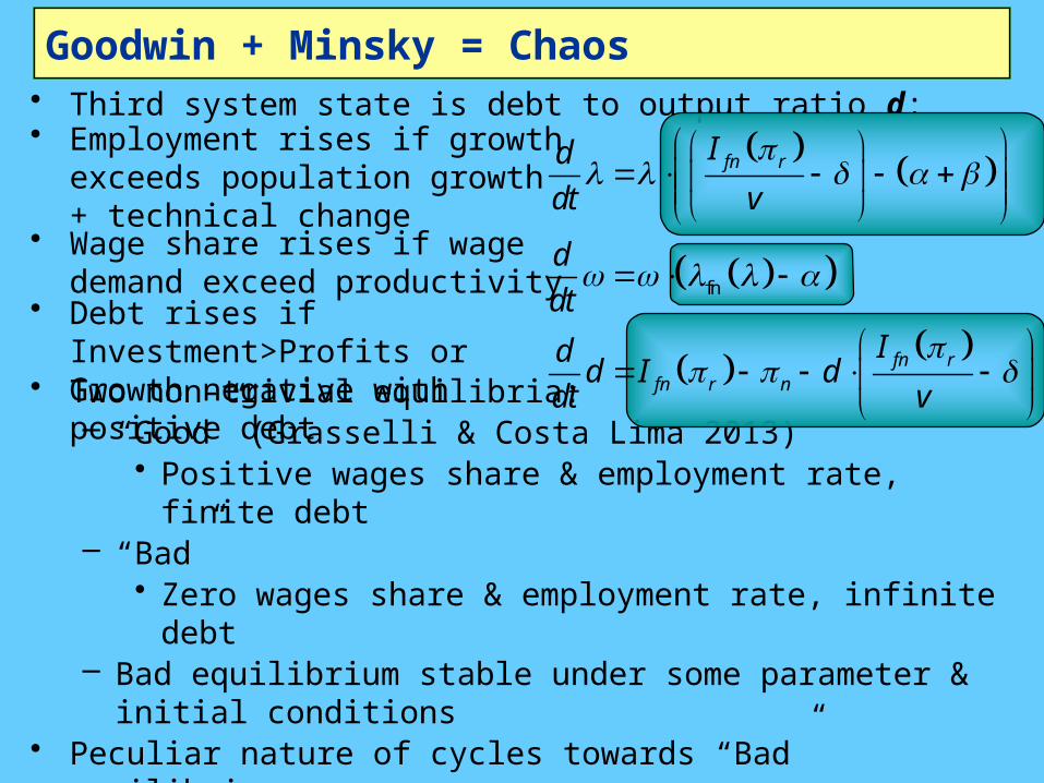
Goodwin + Minsky = Chaos• Third system state is debt to output ratio d:

fn

fn r

fn rfn r n

Id

dt v

d

dt

Idd I d

dt v

• Two non-trivial equilibria:– “Good” (Grasselli & Costa Lima 2013)

• Positive wages share & employment rate, finite debt– “Bad”

• Zero wages share & employment rate, infinite debt– Bad equilibrium stable under some parameter & initial

conditions• Peculiar nature of cycles towards “Bad” equilibrium

– Debt to GDP rises– Cycles in employment & wages diminish and then grow– Wages share of output declines…

• Employment rises if growth exceeds population growth + technical change

• Wage share rises if wage demand exceed productivity

• Debt rises if Investment>Profits or Growth negative with positive debt

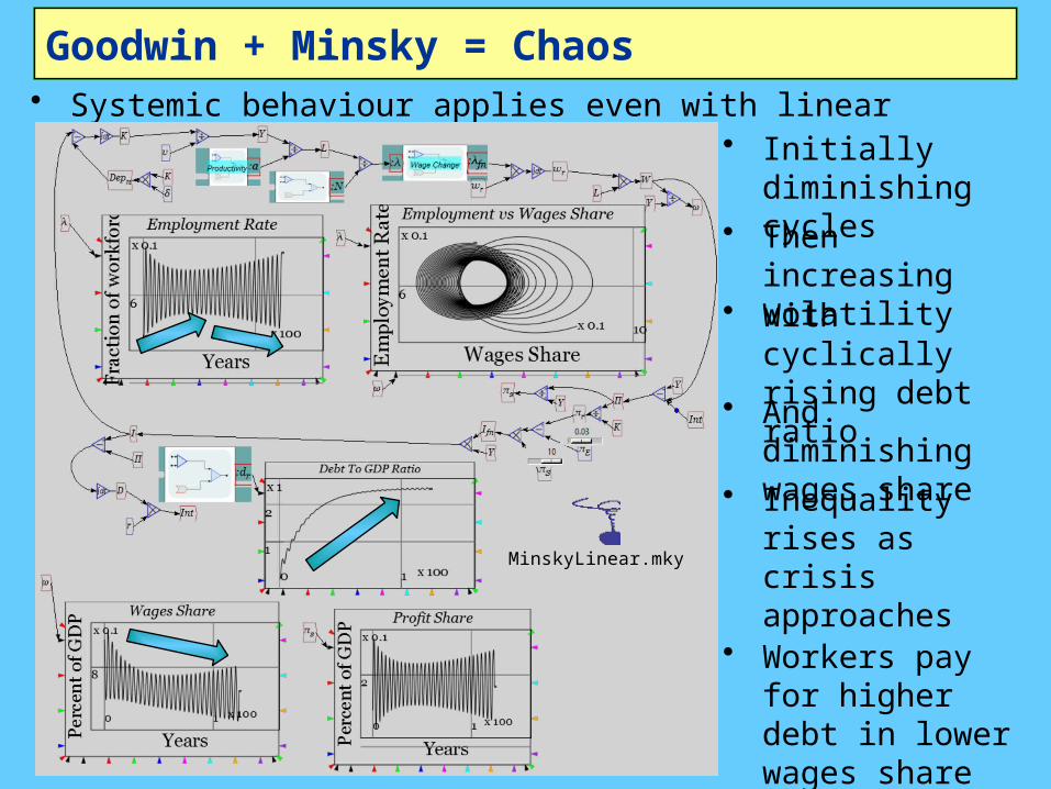
Goodwin + Minsky = Chaos• Systemic behaviour applies even with linear behavioural

functions… • Initially diminishing cycles• Then increasing volatility

• With cyclically rising debt ratio

• And diminishing wages share

• Inequality rises as crisis approaches

• Workers pay for higher debt in lower wages share

• Even though they do not borrow…

MinskyLinear.mky

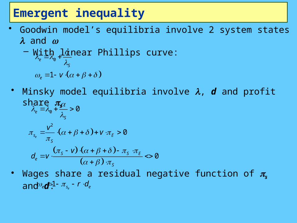
Emergent inequality• Goodwin model’s equilibria involve 2 system states l and w

– With linear Phillips curve:

0

1

eS

e v

• Minsky model equilibria involve l, d and profit share ps

0

2

0

0

0

e

eS

s ES

S S Ee

S

vv

vd v

• Wages share a residual negative function of ps and d:

1ee s er d

Emergent inequality• Model dynamics involve

– Cycles around equilibrium values for l and pS

– Falling wages share compensates for rising debt servicing costs

• Declining workers’ share lulls capitalists into false sense of security as debt level rises

– Profits cyclical around equilibrium level…– Until exponential debt relation overwhelms falling wages

share– Then collapse: zero employment, zero wages, infinite

debt, infinitely negative profit rate– Fundamentally unstable dynamics of pure credit

economy without government or bankruptcy…

Minsky’s “Financial Instability Hypothesis”

• Minsky cycle in extended model

GoodwinMinskyNonlinear.mky

Minsky’s “Financial Instability Hypothesis”

• 1995 paper Conclusion (written in 1992 before end of 1990s recession):– “From the perspective of economic theory and policy,

this vision of a capitalist economy with finance requires us to go beyond that habit of mind which Keynes described so well, the excessive reliance on the (stable) recent past as a guide to the future.

– The chaotic dynamics explored in this paper should warn us against accepting a period of relative tranquility in a capitalist economy as anything other than a lull before the storm.”

• Post 1992 economic history…

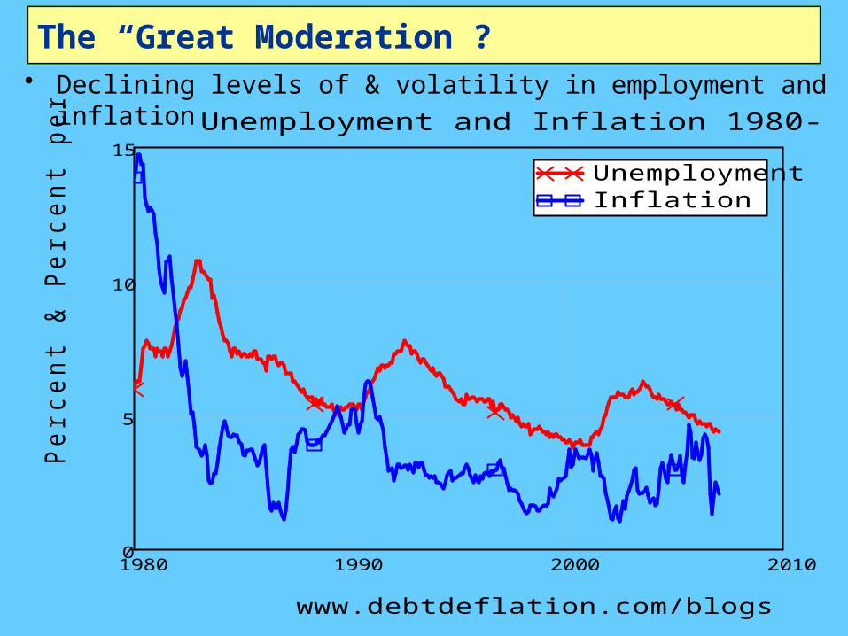
The “Great Moderation”?• Declining levels of & volatility in employment and inflation

1980 1990 2000 20100

5

10

15

UnemploymentInflation

Unemployment and Inflation 1980-2008

www.debtdeflation.com/blogs

Perc

en

t &

Perc

en

t p

er

year

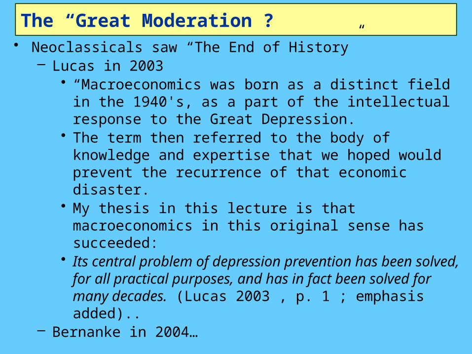
The “Great Moderation”?• Neoclassicals saw “The End of History”

– Lucas in 2003• “Macroeconomics was born as a distinct field in the

1940's, as a part of the intellectual response to the Great Depression.

• The term then referred to the body of knowledge and expertise that we hoped would prevent the recurrence of that economic disaster.

• My thesis in this lecture is that macroeconomics in this original sense has succeeded:

• Its central problem of depression prevention has been solved, for all practical purposes, and has in fact been solved for many decades. (Lucas 2003 , p. 1 ; emphasis added)..

– Bernanke in 2004…

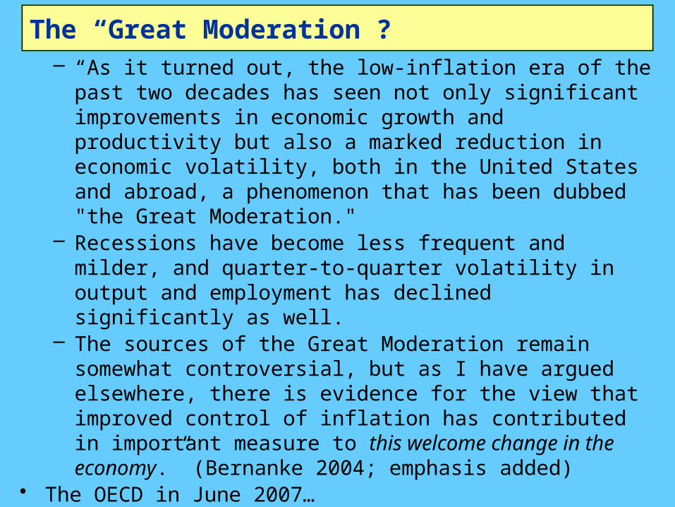
The “Great Moderation”?– “As it turned out, the low-inflation era of the past two

decades has seen not only significant improvements in economic growth and productivity but also a marked reduction in economic volatility, both in the United States and abroad, a phenomenon that has been dubbed "the Great Moderation."

– Recessions have become less frequent and milder, and quarter-to-quarter volatility in output and employment has declined significantly as well.

– The sources of the Great Moderation remain somewhat controversial, but as I have argued elsewhere, there is evidence for the view that improved control of inflation has contributed in important measure to this welcome change in the economy.” (Bernanke 2004; emphasis added)

• The OECD in June 2007…

The “Great Moderation”?• “In its Economic Outlook last Autumn, the OECD took

the view that the US slowdown was not heralding a period of worldwide economic weakness, unlike, for instance, in 2001.

• Rather, a “smooth” rebalancing was to be expected, with Europe taking over the baton from the United States in driving OECD growth.

• Recent developments have broadly confirmed this prognosis. Indeed, the current economic situation is in many ways better than what we have experienced in years. Against that background, we have stuck to the rebalancing scenario.

• Our central forecast remains indeed quite benign: a soft landing in the United States, a strong and sustained recovery in Europe, a solid trajectory in Japan and buoyant activity in China and India. In line with recent trends, sustained growth in OECD economies would be underpinned by strong job creation and falling unemployment.” (Cotis 2007 , p. 7)

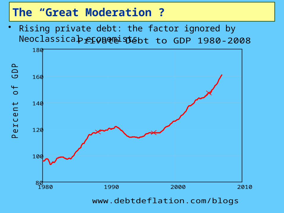
The “Great Moderation”?• Rising private debt: the factor ignored by Neoclassical

economists

1980 1990 2000 201080

100

120

140

160

180

Private Debt to GDP 1980-2008

www.debtdeflation.com/blogs

Per

cen

t o

f G

DP

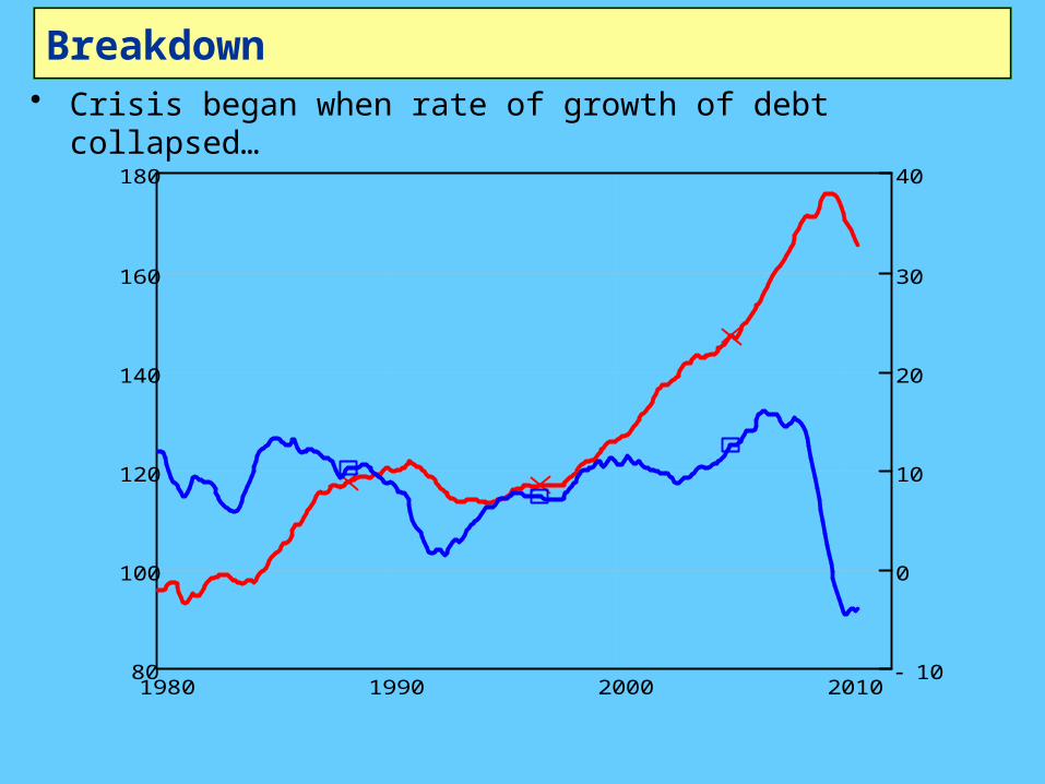
Breakdown• Crisis began when rate of growth of debt collapsed…

1980 1990 2000 201080

100

120

140

160

180

10

0

10

20

30

40

LevelRate of Change

Private debt level & growth rate

www.debtdeflation.com/blogs

Per

cen

t o

f G

DP

Per

cen

t o

f G

DP

p.a

.

0

Crisis

Breakdown• Unemployment exploded, inflation became deflation

(before rescue)

1980 1990 2000 20105

0

5

10

15

UnemploymentInflation

Unemployment and Inflation 1980-2010

www.debtdeflation.com/blogs

Perc

en

t &

Perc

ent

per

year

0

Crisis

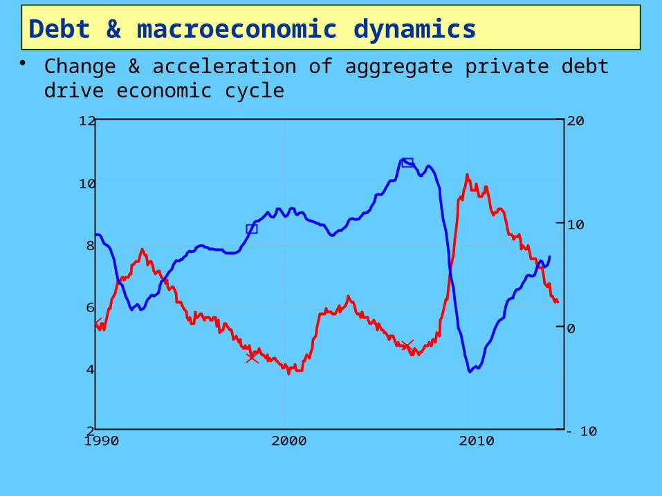
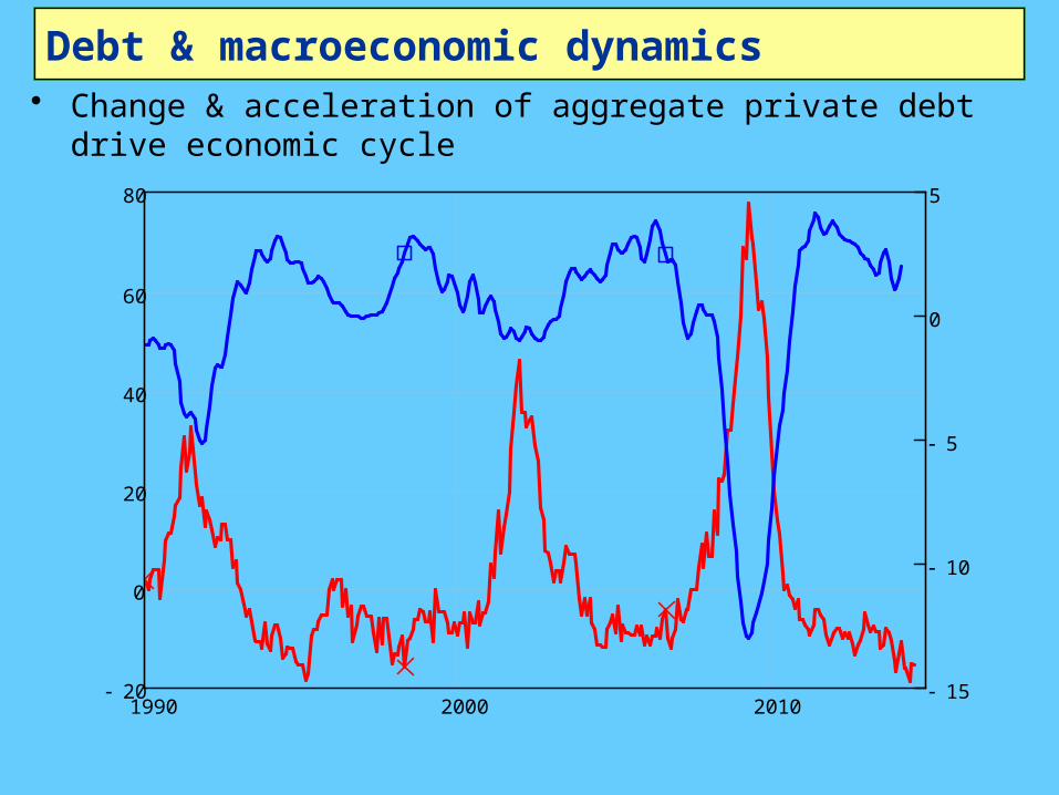
Debt & macroeconomic dynamics• Change & acceleration of aggregate private debt drive

economic cycle

1990 2000 20102

4

6

8

10

12

10

0

10

20

UnemploymentChange in Debt

Unemployment and Change in Debt 1990-Now

www.debtdeflation.com/blogs

Per

cen

t

Per

cen

t of

GD

P p

er y

ear

0

Crisis

Correlation -0.9

Debt & macroeconomic dynamics• Change & acceleration of aggregate private debt drive

economic cycle

1990 2000 201020

0

20

40

60

80

15

10

5

0

5

Unemployment ChangeDebt Acceleration

Change in Unemployment and Debt Acceleration 1990-Now

www.debtdeflation.com/blogs

Per

cent

per

yea

r

Per

cent

of

GD

P pe

r ye

ar p

er y

ear

0

Crisis

Correlation -0.89

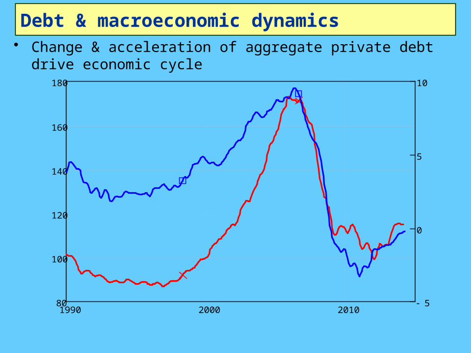
Debt & macroeconomic dynamics• Change & acceleration of aggregate private debt drive

economic cycle

1990 2000 201080

100

120

140

160

180

5

0

5

10

IndexMortgage Change

Real House Price and Change in Mortgage Debt 1990-Now

www.debtdeflation.com/blogs

Infl

atio

n A

djus

ted

Inde

x

Per

cent

of

GD

P pe

r ye

ar

0

Crisis

Correlation 0.61

Debt & macroeconomic dynamics• Change & acceleration of aggregate private debt drive

economic cycle

1990 2000 201030

20

10

0

10

20

6

4

2

0

2

4

House Price Index ChangeMortgage Acceleration

Change in House Prices and Mortgage Acceleration 1990-Now

www.debtdeflation.com/blogs

Infl

atio

n-ad

just

ed p

erce

nt p

er y

ear

Per

cent

of

GD

P pe

r ye

ar p

er y

ear

0

Crisis

Correlation 0.79

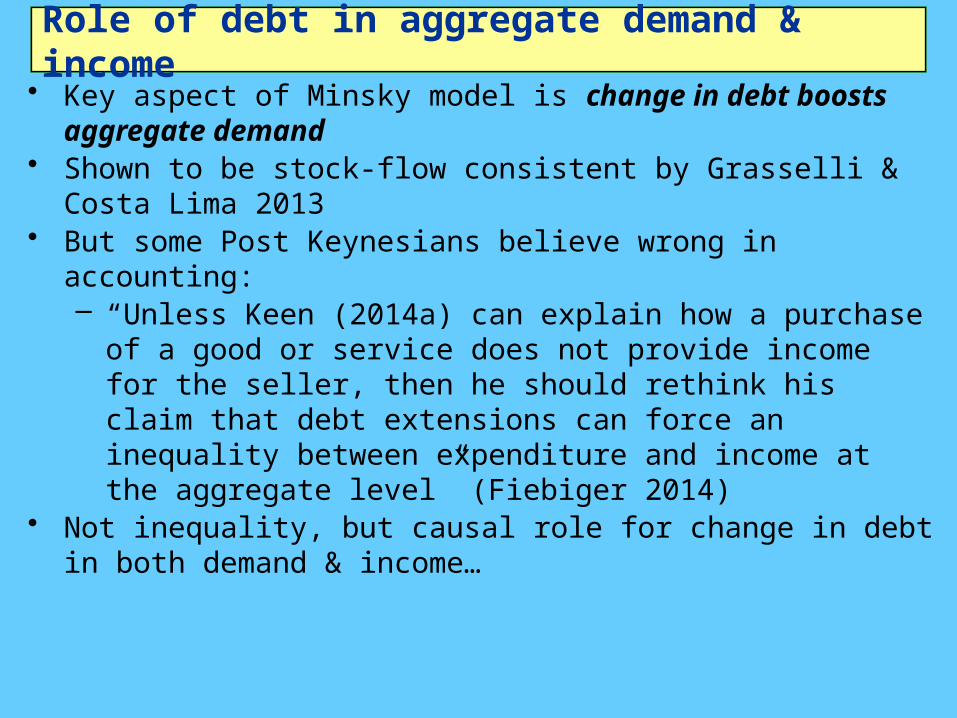
Role of debt in aggregate demand & income

• Key aspect of Minsky model is change in debt boosts aggregate demand

• Shown to be stock-flow consistent by Grasselli & Costa Lima 2013

• But some Post Keynesians believe wrong in accounting:– “Unless Keen (2014a) can explain how a purchase of a

good or service does not provide income for the seller, then he should rethink his claim that debt extensions can force an inequality between expenditure and income at the aggregate level” (Fiebiger 2014)

• Not inequality, but causal role for change in debt in both demand & income…

Role of debt in aggregate demand & income

• Deriving role of change in debt in aggregate demand & income from an expenditure table– 3 sectors, 3 situations

• No borrowing is possible (“Say’s Law”)• Borrowing from other agents is possible (“Loanable

Funds”)• Banks lend to non-banks (“Endogenous Money”)

– 2 types of expenditure:• Financed out of existing money

– Exy: Expenditure by sector x to buy from sector y• Financed by borrowing

– DD for single instance– dD/dt for flow of debt in continuous time

Role of debt in aggregate demand & income

• Expenditure Table– Rows show expenditure by each sector– Columns show net income– Negative sum of diagonal is aggregate demand– Sum of off-diagonal elements is aggregate income

SL

"Activity\Sector"

"Expenditure"

"Expenditure"

"Expenditure"

"S1"

E1 2 E

1 3

E2 1

E3 1

"S2"

E1 2

E2 1 E

2 3

E3 2

"S3"

E1 3

E2 3

E3 1 E

3 2

E

• Simplest “Say’s Law” (really “demand creates its own supply…”)

Sector 1 Net Incom

e

Aggregate demandAggregate income

Aggregate income

• Aggregate demand AY SL( ) E

1 2 E2 1 E

1 3 E3 1 E

2 3 E3 2• Aggregate

income

AD SL( ) E1 2 E

2 1 E1 3 E

3 1 E2 3 E

3 2

Role of debt in aggregate demand & income

• Loanable Funds: Sector 1 borrows DD from Sector 2– Sector 1 spends borrowed funds in proportion a,1-a on 2

& 3– Sector 2 spends that much less in proportions b,1-b on

1 and 3LF

"Activity\Sector"

"Expenditure"

"Expenditure"

"Expenditure"

"S1"

E1 2 D E

1 3 1 ( ) D

E2 1 D

E3 1

"S2"

E1 2 D

E2 1 D E

2 3 1 ( ) D

E3 2

"S3"

E1 3 1 ( ) D

E2 3 1 ( ) D

E3 1 E

3 2( )

EE

In Endogenous money, the ?D that increases Sector 1's expenditure emanates from a loan from the banking sector (not shown here) whichincreases the banking sector's assets and liabilities equally. • Aggregate

demand• Aggregate income

AD LF( ) collect D E1 2 E

2 1 E1 3 E

3 1 E2 3 E

3 2

AY LF( ) collect D E1 2 E

2 1 E1 3 E

3 1 E2 3 E

3 2

• Increase in spending power of borrower offset by decrease in spending power of lender

• Neoclassicals logically correct that, if this accurately describes lending, “pure redistributions should have no significant macroeconomic effects”…

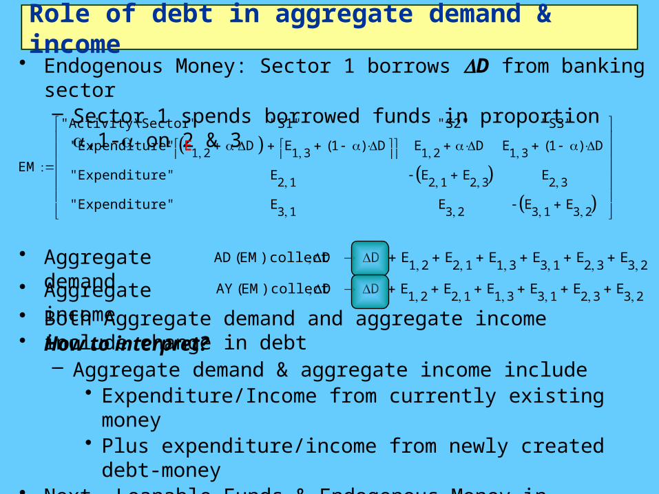
Role of debt in aggregate demand & income

• Endogenous Money: Sector 1 borrows DD from banking sector– Sector 1 spends borrowed funds in proportion a,1-a on 2

& 3EM

"Activity\Sector"

"Expenditure"

"Expenditure"

"Expenditure"

"S1"

E1 2 D E

1 3 1 ( ) D

E2 1

E3 1

"S2"

E1 2 D

E2 1 E

2 3

E3 2

"S3"

E1 3 1 ( ) D

E2 3

E3 1 E

3 2

EE

• Aggregate demand• Aggregate income

AD EM( ) collect D D E1 2 E

2 1 E1 3 E

3 1 E2 3 E

3 2

Income equals expenditureAY EM( ) collect D D E1 2 E

2 1 E1 3 E

3 1 E2 3 E

3 2

Expenditure• Both Aggregate demand and aggregate income include change in debt• How to interpret?– Aggregate demand & aggregate income include

• Expenditure/Income from currently existing money• Plus expenditure/income from newly created debt-

money• Next, Loanable Funds & Endogenous Money in continuous

time

Role of debt in aggregate demand & income

• Loanable funds: flow of lending from Sector 2 to Sector 1

"Activity\Sector"

"Expenditure"

"Expenditure"

"Expenditure"

S1

S1

12

S1

13

tDd

d

rL D

S2

21

tDd

d

S3

31

S2

S1

12

tDd

d rL D

S2

21

S2

23

tDd

d

S3

32

S3

S1

131 ( )

tDd

d

S2

231 ( )

tDd

d

S3

31

S3

32

• Aggregate demand

• Aggregate income

AY LF2 simplify

collect S1 S2 S31

12

1

13

S11

21

1

23

S21

31

1

32

S3 D rL

AD LF2 simplify

collect S1 S2 S31

12

1

13

S11

21

1

23

S21

31

1

32

S3 D rL

• Interest is part of aggregate demand/income

• Sector 1 pays interest to Sector 2

Role of debt in aggregate demand & income

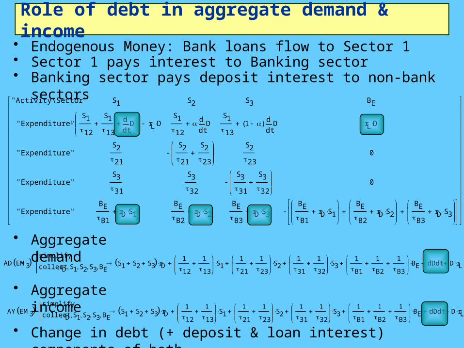
• Endogenous Money: Bank loans flow to Sector 1

"Activity\Sector"

"Expenditure"

"Expenditure"

"Expenditure"

"Expenditure"

S1

S1

12

S1

13

tDd

d

rL D

S2

21

S3

31

BE

B1rD S1

S2

S1

12

tDd

d

S2

21

S2

23

S3

32

BE

B2rD S2

S3

S1

131 ( )

tDd

d

S2

23

S3

31

S3

32

BE

B3rD S3

BE

rL D

0

0

BE

B1rD S1

BE

B2rD S2

BE

B3rD S3

• Sector 1 pays interest to Banking sector• Banking sector pays deposit interest to non-bank sectors

• Aggregate demand

• Aggregate income

AD EM3 simplify

collect rD S1 S2 S3 BE S1 S2 S3 rD1

12

1

13

S11

21

1

23

S21

31

1

32

S31

B1

1

B2

1

B3

BE dDdt D rL

AY EM3 simplify

collect rD S1 S2 S3 BE S1 S2 S3 rD1

12

1

13

S11

21

1

23

S21

31

1

32

S31

B1

1

B2

1

B3

BE dDdt D rL

• Change in debt (+ deposit & loan interest) components of both

Role of debt in aggregate demand & income

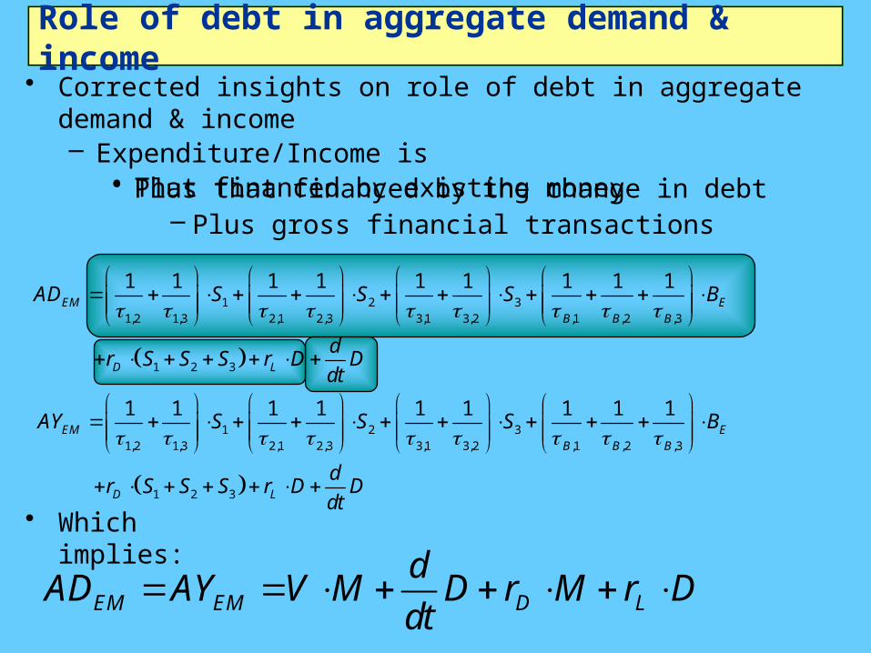
• Corrected insights on role of debt in aggregate demand & income– Expenditure/Income is

• That financed by existing money

1 2 31,2 1,3 2,1 2,3 3,1 3,2 ,1 ,2 ,3

1 2 3

1 2 31,2 1,3 2,1 2,3 3,1 3,2

1 1 1 1 1 1 1 1 1

1 1 1 1 1 1 1

EM EB B B

D L

EM

AD S S S B

dr S S S r D D

dt

AY S S S

,1 ,2 ,3

1 2 3

1 1E

B B B

D L

B

dr S S S r D D

dt

• Plus that financed by the change in debt– Plus gross financial transactions

EM EM D L

dAD AY V M D r M r D

dt

• Which implies:

Role of debt in aggregate demand & income

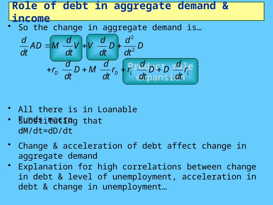
• So the change in aggregate demand is…2

2

D D L L

d d d dAD M V V D D

dt dt dt dtd d d d

r D M r r D D rdt dt dt dt

• All there is in Loanable Funds macro

• Change & acceleration of debt affect change in aggregate demand

• Explanation for high correlations between change in debt & level of unemployment, acceleration in debt & change in unemployment…

Product rule expansion

• Substituting that dM/dt=dD/dt

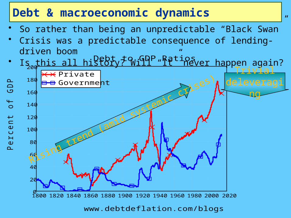
Debt & macroeconomic dynamics• So rather than being an unpredictable “Black Swan”• Crisis was a predictable consequence of lending-driven

boom• Is this all history? Will “It” never happen again?

1800 1820 1840 1860 1880 1900 1920 1940 1960 1980 2000 20200

20

40

60

80

100

120

140

160

180

200

PrivateGovernment

Debt to GDP Ratios

www.debtdeflation.com/blogs

Per

cen

t o

f G

DP

Rising tre

nd (amid systemic crise

s)

Trivial deleveragin

g

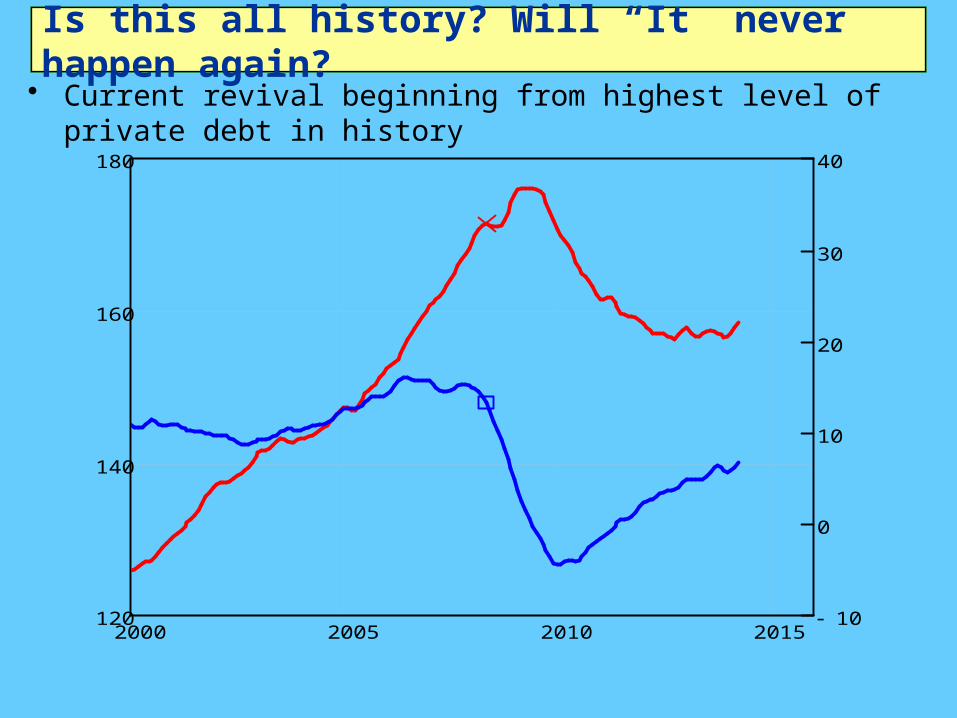
Is this all history? Will “It” never happen again?

• Current revival beginning from highest level of private debt in history

2000 2005 2010 2015120

140

160

180

10

0

10

20

30

40

LevelRate of Change

Private debt level & growth rate

www.debtdeflation.com/blogs

Per

cen

t o

f G

DP

Per

cen

t o

f G

DP

p.a

.

0

Crisis • “It” will happen again, & sooner than last time (15 years 1992-2007)

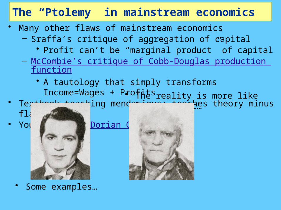
The “Ptolemy” in mainstream economics• Many other flaws of mainstream economics

– Sraffa’s critique of aggregation of capital• Profit can’t be “marginal product” of capital

– McCombie’s critique of Cobb-Douglas production function

• A tautology that simply transforms Income=Wages + Profits

• Textbook teaching mendacious: teaches theory minus flaws• You are shown Dorian Gray

• The reality is more like his portrait…

• Some examples…

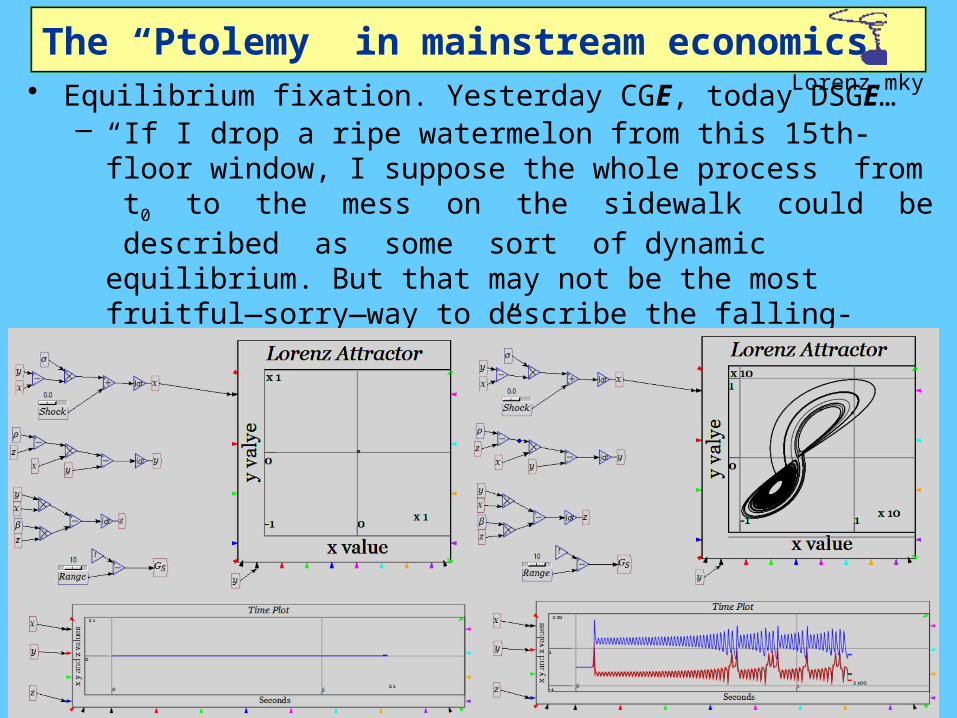
The “Ptolemy” in mainstream economics• Equilibrium fixation. Yesterday CGE, today DSGE…

– “If I drop a ripe watermelon from this 15th-floor window, I suppose the whole process from t0 to the mess on the sidewalk could be described as some sort of dynamic equilibrium. But that may not be the most fruitful—sorry—way to describe the falling-watermelon phenomenon.” (Solow “Dumb & Dumber in Macro”)

• Modern dynamics is “far from equilibrium”… E.g., Lorenz’s “butterfly”

Lorenz.mky

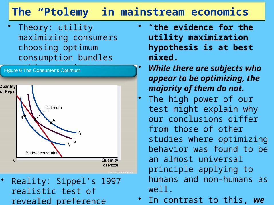
The “Ptolemy” in mainstream economics• Theory: utility maximizing

consumers choosing optimum consumption bundles subject to income constraint

• Reality: Sippel’s 1997 realistic test of revealed preference theory:

• “the evidence for the utility maximization hypothesis is at best mixed.

• While there are subjects who appear to be optimizing, the majority of them do not.

• The high power of our test might explain why our conclusions differ from those of other studies where optimizing behavior was found to be an almost universal principle applying to humans and non-humans as well.

• In contrast to this, we would like to stress the diversity of individual behavior and call the universality of the maximizing principle into question…”

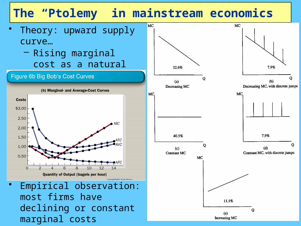
The “Ptolemy” in mainstream economics• Theory: upward supply

curve…– Rising marginal cost as

a natural consequence of fixed & variable inputs…

• Empirical observation: most firms have declining or constant marginal costs

• Alan Blinder 1999 survey:

The “Ptolemy” in mainstream economics• “Another very common assumption of economic theory is

that marginal cost is rising. This notion is enshrined in every textbook and employed in most economic models.

• It is the foundation of the upward-sloping supply curve.• However, as we have noted already, Hall has used constant

MC as the basis for one family of models of price stickiness. What do business people have to say about their own cost structures?”

• “Firms report having very high fixed costs—roughly 40 percent of total costs on average.

• And many more companies state that they have falling, rather than rising, marginal cost curves. While there are reasons to wonder whether respondents interpreted these questions about costs correctly,

• their answers paint an image of the cost structure of the typical firm that is very different from the one immortalized in textbooks.”– Alan Blinder, ex-Vice President of American Economic

Association– (Click here for downloadable chapters—Chapter 4 the

core)

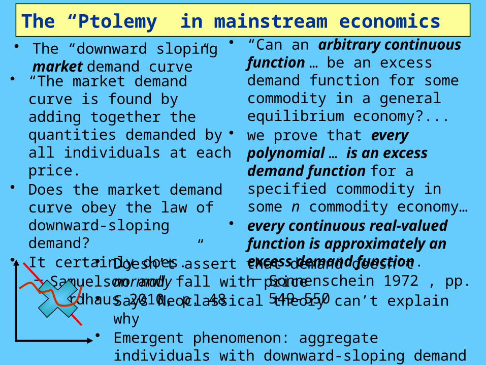
The “Ptolemy” in mainstream economics• The “downward sloping

market demand curve”• “The market demand curve

is found by adding together the quantities demanded by all individuals at each price.

• Does the market demand curve obey the law of downward-sloping demand?

• It certainly does.”– Samuelson and

Nordhaus 2010, p. 48

• “Can an arbitrary continuous function … be an excess demand function for some commodity in a general equilibrium economy?...

• we prove that every polynomial … is an excess demand function for a specified commodity in some n commodity economy…

• every continuous real-valued function is approximately an excess demand function.– Sonnenschein 1972 , pp.

549-550

• Doesn’t assert that demand doesn’t normally fall with price

• Says Neoclassical theory can’t explain why• Emergent phenomenon: aggregate individuals

with downward-sloping demand curves…• Get any (polynomial) shaped demand curve at all

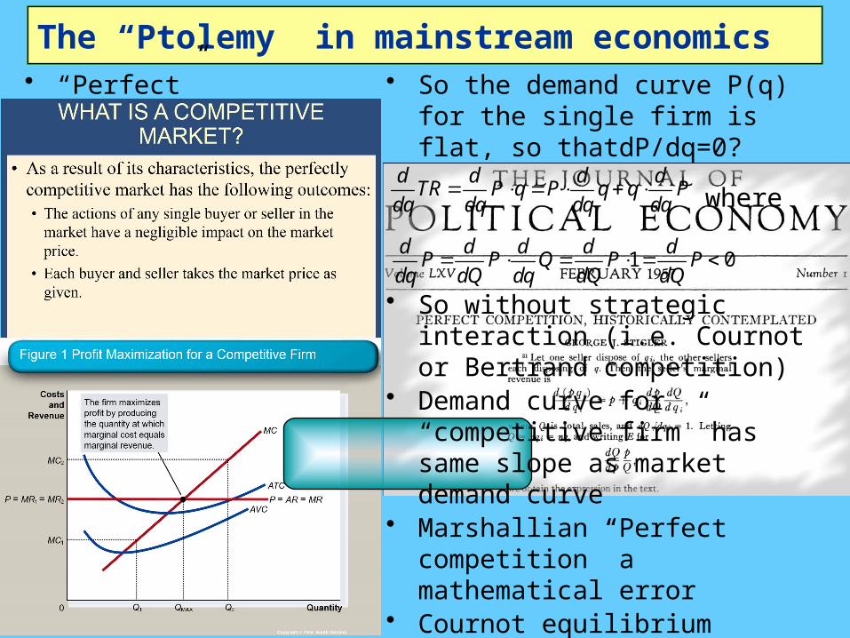
The “Ptolemy” in mainstream economics• “Perfect”

competition…• So the demand curve P(q) for

the single firm is flat, so thatdP/dq=0?

• Not according to Stigler…d d d dTR P q P q q P

dq dq dq dq where

1 0d d d d dP P Q P P

dq dQ dq dQ dQ

• So without strategic interaction (i.e. Cournot or Bertrand competition)

• Demand curve for “competitive firm” has same slope as market demand curve

• Marshallian “Perfect competition” a mathematical error

• Cournot equilibrium locally unstable (mathematically, & not equilibrium in repeated games)

• See Keen & Standish 2010

Conclusion• We need an empirically realistic, logically sound, theory of

economics• Neoclassical equilibrium/barter model like Ptolemy’s theory

of cosmos– We need a Copernican replacement

• In the meantime, you should learn all theories, not just Neoclassical– And if that doesn’t happen at your University, then…

For a pluralist education in economics

Come to Kingston

School of Economics, History & Politics

KingstonUniversityLondon

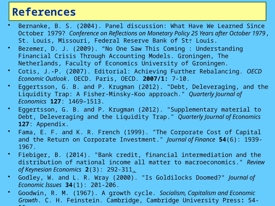
References• Bernanke, B. S. (2004). Panel discussion: What Have We Learned Since October

1979? Conference on Reflections on Monetary Policy 25 Years after October 1979, St. Louis, Missouri, Federal Reserve Bank of St. Louis.

• Bezemer, D. J. (2009). “No One Saw This Coming”: Understanding Financial Crisis Through Accounting Models. Groningen, The Netherlands, Faculty of Economics University of Groningen.

• Cotis, J.-P. (2007). Editorial: Achieving Further Rebalancing. OECD Economic Outlook. OECD. Paris, OECD. 2007/1: 7-10.

• Eggertsson, G. B. and P. Krugman (2012). "Debt, Deleveraging, and the Liquidity Trap: A Fisher-Minsky-Koo approach." Quarterly Journal of Economics 127: 1469–1513.

• Eggertsson, G. B. and P. Krugman (2012). "Supplementary material to Debt, Deleveraging and the Liquidity Trap." Quarterly Journal of Economics 127: Appendix.

• Fama, E. F. and K. R. French (1999). "The Corporate Cost of Capital and the Return on Corporate Investment." Journal of Finance 54(6): 1939-1967.

• Fiebiger, B. (2014). "Bank credit, financial intermediation and the distribution of national income all matter to macroeconomics." Review of Keynesian Economics 2(3): 292-311.

• Godley, W. and L. R. Wray (2000). "Is Goldilocks Doomed?" Journal of Economic Issues 34(1): 201-206.

• Goodwin, R. M. (1967). A growth cycle. Socialism, Capitalism and Economic Growth. C. H. Feinstein. Cambridge, Cambridge University Press: 54-58.

• Keen, S. (1995). "Finance and Economic Breakdown: Modeling Minsky's 'Financial Instability Hypothesis.'." Journal of Post Keynesian Economics 17(4): 607-635.

References• Keen, S. (2006). "The Recession We Can't Avoid?" Steve Keen's Debtwatch, from

http://debtdeflation.com/blogs/wp-content/uploads/2007/03/SteveKeenDebtReportNovember2006.pdf.

• Keen, S. (2007). Deeper in Debt: Australia's addiction to borrowed money. Occasional Papers. Sydney, Centre for Policy Development.

• Keen, S. (2014). “Endogenous money and effective demand.” Review of Keynesian Economics 2(3): 271–291.

• Krugman, P. (2012). End this Depression Now! New York, W.W. Norton.• Lavoie, M. (2014). "A comment on ‘Endogenous money and effective demand’: a

revolution or a step backwards?" Review of Keynesian Economics 2(3): 321 - 332.• McLeay, M., A. Radia and R. Thomas (2014). "Money creation in the modern

economy." Bank of England Quarterly Bulletin 2014 Q1: 14-27.• Martin, F. (2013). Money: The Unauthorised Biography. London, The Bodley Head

Ltd.• Minsky, H. P. (1982). Can "it" happen again? : essays on instability and finance.

Armonk, N.Y., M.E. Sharpe.• Wray, L. R. (2002). "What Happened to Goldilocks? A Minskian Framework." Journal

of Economic Issues 36(2): 383-391.

Date Unemployment RateUnemployment change % p.a.CPI Inflation p.a.Private DebtGovernment DebtPrivate Debt change p.a.Government Debt change p.a.Private Debt acceleration p.a.Government Debt acceleration p.a.GDP Private debt % GDPGovernment debt % GDPPrivate Debt change p.a % GDPGovernment Debt change p.a % GDPHouse Price Index CPI adjustedChange House Price Index p.a.Mortgage DebtMortgage Debt change p.a.1790 187

1790.083 76.6772 188.2925 40.722381790.167 77.25289 189.6077 40.74355

1790.25 77.79589 190.9453 40.742491790.333 78.30621 192.3056 40.719671790.417 78.78384 193.6884 40.67556

1790.5 79.22878 195.0938 40.610611790.583 79.64104 196.5217 40.525311790.667 80.02061 197.9722 40.42012

1790.75 80.3675 199.4453 40.29551790.833 80.6817 200.941 40.151941790.917 80.96321 202.4592 39.98989

1791 81.21204 204 39.809821791.083 81.42818 4.750983 205.5626 39.61235 2.3112091791.167 81.61272 4.359829 207.1435 39.39912 2.104739

1791.25 81.77102 3.975133 208.7383 39.17395 1.9043631791.333 81.90956 3.603351 210.3426 38.94103 1.7130871791.417 82.03478 3.250941 211.9521 38.7044 1.53381

1791.5 82.15314 2.92436 213.5624 38.46797 1.3693231791.583 82.2711 2.630065 215.1694 38.23551 1.2223231791.667 82.39512 2.374514 216.7685 38.01066 1.095415

1791.75 82.53166 2.164163 218.3554 37.79694 0.9911191791.833 82.68717 2.00547 219.9259 37.59774 0.9118841791.917 82.8681 1.904892 221.4755 37.41637 0.860092

1792 83.08093 1.868887 223 37.25602 0.8380661792.083 83.3321 1.903912 -2.84707 224.5015 37.11873 0.8480621792.167 83.62518 2.012467 -2.34736 226.0082 37.00096 0.89044

1792.25 83.95225 2.181227 -1.79391 227.5548 36.8932 0.958551792.333 84.30247 2.392911 -1.21044 229.1761 36.78502 1.0441371792.417 84.66501 2.630237 -0.6207 230.9067 36.66633 1.139091

1792.5 85.02906 2.875924 -0.04844 232.7814 36.52742 1.2354611792.583 85.38379 3.112689 0.482624 234.835 36.35906 1.3254791792.667 85.71837 3.323251 0.948738 237.1021 36.15252 1.401612

1792.75 86.02199 3.490329 1.326167 239.6174 35.89973 1.4566261792.833 86.28381 3.596641 1.591171 242.4157 35.59333 1.4836671792.917 86.49301 3.624905 1.720013 245.5316 35.22683 1.47635

1793 86.63877 3.55784 1.688953 249 34.79469 1.4288511793.083 86.71026 3.378164 1.474252 252.8447 34.29389 1.3360631793.167 86.70059 3.075405 1.062938 257.0461 33.72959 1.196441

1793.25 86.61858 2.666334 0.485107 261.5738 33.11439 1.0193431793.333 86.477 2.174532 -0.21838 266.3976 32.46162 0.8162731793.417 86.28859 1.623577 -1.00666 271.4871 31.78368 0.598031

1793.5 86.06611 1.037051 -1.83887 276.8118 31.09192 0.3746411793.583 85.82233 0.438535 -2.67415 282.3414 30.39665 0.1553211793.667 85.56998 -0.14839 -3.47164 288.0456 29.7071 -0.05152

1793.75 85.32184 -0.70015 -4.19048 293.8939 29.03152 -0.238231793.833 85.09065 -1.19316 -4.7898 299.8559 28.37718 -0.397911793.917 84.88918 -1.60383 -5.22874 305.9014 27.7505 -0.5243

1794 84.73017 -1.9086 -5.46644 312 27.15711 -0.611731794.083 84.62638 -2.08388 -5.46204 318.1222 26.60185 -0.655051794.167 84.58757 -2.11302 -5.18842 324.2428 26.08773 -0.65168

1794.25 84.61143 -2.00715 -4.67349 330.3373 25.61364 -0.607611794.333 84.69266 -1.78434 -3.95887 336.3815 25.17756 -0.530451794.417 84.82595 -1.46264 -3.08621 342.351 24.77748 -0.42723

1794.5 85.00601 -1.06011 -2.09716 348.2214 24.41149 -0.304431794.583 85.22751 -0.59481 -1.03335 353.9684 24.07772 -0.168041794.667 85.48516 -0.08482 0.063575 359.5676 23.77444 -0.02359

1794.75 85.77366 0.451821 1.151971 364.9947 23.49997 0.1237881794.833 86.08769 0.997041 2.190198 370.2254 23.25278 0.2693071794.917 86.42196 1.53278 3.136615 375.2353 23.03141 0.408485

1795 86.77115 2.040978 3.949578 380 22.83451 0.5370991795.083 87.12996 2.503572 4.587448 384.4974 22.66074 0.6511281795.167 87.49316 2.905586 5.018606 388.7143 22.50835 0.747486

1795.25 87.85581 3.24438 5.251533 392.6393 22.3757 0.8263

Data in presentation: