Case Study 2

The Origins of Maxwell’s Equations

1

Case Study 2

The Origins of Maxwell’s Equations

800 BC: Greek writers describe magnetic materials, the name being derived from thematerial magnetite, which was known to attract iron in its natural state – it was minedin the Greek province of Magnesia in Thessaly.

They also knew about static electricity which arises when amber rods are rubbed withfur – the Greek word for amber is elektron.

The first systematic study of magnetic and electric phenomena was published in 1600by William Gilbert in De Magnete, Magnetisque Corporibus, et de Magno MagneteTellure.

2

Early History

• Benjamin Franklin systematised the laws of electrostatics and defined the conceptsof positive and negative electric charges.

• In 1767, Joseph Priestly showed that there are no electric forces inside aconducting sphere, the forerunner of the Williams, Faller and Hall experiment of1971 which demonstrated the the remarkable precision of the inverse square law ofelectrostatics.

• In the period 1779-1780, Charles-Augustin Coulomb derived experimentally hisLaws of Electrostatics and Magnetostatics:

f =q1q2

4πǫ0r2ir and f =

µ0p1p2

4πr2ir,

where ir is the unit vector directed radially away from either charge in the directionof the other.

3

Mathematics of Electrostatics and Magnetostatics

In 1812, Simeon-Denis Poisson published his famous Memoire sur la Distribution del’Electricite a la Surface des Corps Conducteurs and wrote down Poisson’s equation forthe electrostatic potential

∂2V

∂x2+

∂2V

∂y2+

∂2V

∂z2= −

ρe

ǫ0,

where ρe is the electric charge density distribution. The electric field strength E is givenby

E = −gradV.

4

Mathematics of Electrostatics and Magnetostatics

In 1812, Simeon-Denis Poisson published his famous Memoire sur la Distribution del’Electricite a la Surface des Corps Conducteurs and wrote down Poisson’s equation forthe electrostatic potential V

∂2V

∂x2+

∂2V

∂y2+

∂2V

∂z2= −

ρe

ǫ0,

where ρe is the electric charge density distribution. The electric field strength E is givenby

E = −gradV.

In 1826, the corresponding expressions for the magnetic flux density B in terms of themagnetostatic potential Vmag were presented:

∂2Vmag

∂x2+

∂2Vmag

∂y2+

∂2Vmag

∂z2= 0,

where the magnetic flux density B is given by

B = −µ0 gradVmag.

5

Luigi Galvani

Luigi Galvani discovered thatelectrical effects couldstimulate the muscularcontraction of frogs’ legs. In1791, he showed that, whentwo dissimilar metals wereused to make the connectionbetween nerve and muscle,the same muscularcontraction was observed.This was the discovery ofanimal electricity.

6

Alessandro Volta

Alessandro Volta suspected that theelectric current was associated with thepresence of different metals in contactwith a moist body. In 1800, he built whatbecame known as a voltaic pile,consisting of interleaved layers ofcopper and zinc separated by layers ofpasteboard soaked in a conductingliquid. This led to his construction of hiscrown of cups, which resembles amodern car battery.The most important outcome was thediscovery of a controllable source ofelectric current.

7

Cultural ResonancesMary Shelley’s FrankensteinThis book was written in 1816. In thepreface, the monster was said to berevived by galvanism.

8

Cultural ResonancesMary Shelley’s FrankensteinThis book was written in 1816. In thepreface, the monster was said to berevived by galvanism.

Mozart’s Cosi fan TuttiThis opera was first performed in 1791.The heavily disguised Ferrando andGiuglielmo are revived by magnetismand galvanism.

9

Currents and Magnetism

1820 Hans-Christian Øersted: there is always a magnetic field associated with anelectric current – the beginning of the science of electromagnetism.

1820 Jean-Baptiste Biot (1774–1862) and Felix Savart (1791–1841) discovered thedependence of the strength of the magnetic field at distance r from a current elementof length dl in which a current I is flowing, the Biot-Savart law

dB =µ0I dl × r

4πr3.

Andre-Marie Ampere (1775–1836) extended the Biot-Savart law to relate the currentflowing though a closed loop to the integral of the component of the magnetic fluxdensity around the loop, Ampere’s law.

∫C

B · ds = µ0Ienclosed.

10

Currents and Magnetism

In 1825, Ampere

• represented the magnetic field of a current loop by an equivalent magnetic shell.

• formulated the equation for the force between two current elements, dl1 and dl2

carrying currents I1 and I2 ;

dF 2 =µ0I1I2 dl1 × (dl2 × r)

4πr3.

1827, Georg Simon Ohm (1787–1854) formulated the relation between potentialdifference V and the current I, Ohm’s law, V = RI.

All these results were known by 1830 and comprise the whole of static electricity, theforces between stationary charges, magnets and currents.

11

Michael FaradayMathematics without Mathematics

Maxwell’s equations deal withtime-varying phenomena. Over thesucceeding 20 years, all the basicexperimental features of time-varyingelectric and magnetic fields wereestablished. The hero of this story isMichael Faraday (1791–1867), anexperimenter of genius.

In 1820, at the suggestion of HumphryDavy, Faraday surveyed the manyarticles submitted to the scientificjournals describing electromagneticeffects and began his systematic studyof electromagnetic phenomena.

12

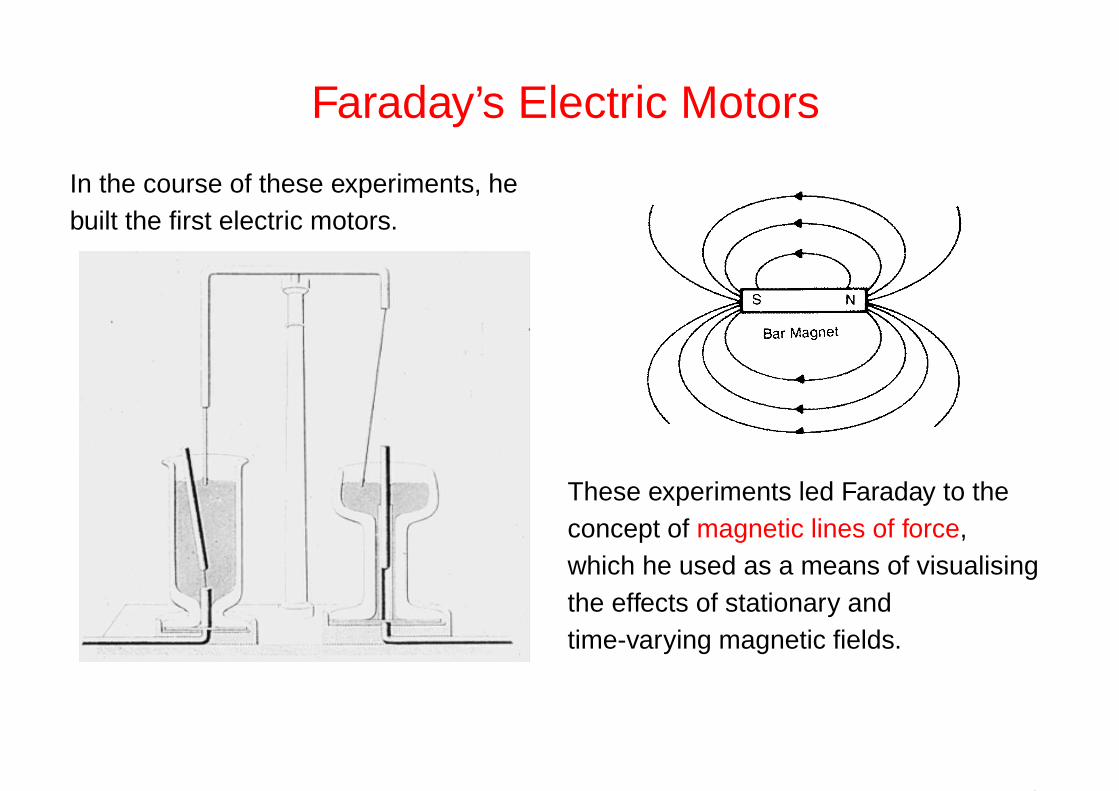
Faraday’s Electric Motors

In the course of these experiments, hebuilt the first electric motors.

These experiments led Faraday to theconcept of magnetic lines of force,which he used as a means of visualisingthe effects of stationary andtime-varying magnetic fields.

13

The Discovery of Electromagnetic Induction

In 1831, Faraday heard about JosephHenry’s experiments in Albany, NewYork with very powerful electromagnets.He had the idea of observing the strainin the material of the electromagnetcaused by the lines of force. He built astrong electromagnet by winding aninsulating wire, through which a currentcould be passed, onto a thick iron ring.The effects of the strain were to bedetected with another winding on thering attached to a galvanometer.

14

The Discovery of Electromagnetic Induction

The experiment was conducted on 29August 1931 and is recorded in Fara-day’s laboratory notebooks. When theprimary circuit was closed, there was adisplacement of the galvanometer nee-dle in the secondary winding. Deflec-tions of the galvanometer were only ob-served when the current in the electro-magnet was switched on and off. Thiswas the discovery of electromagnetic in-duction.

15

The Invention of the Dynamo

There followed a magnificent series ofexperiments• He tried coils of different shapes

and sizes and discovered that theiron bar was not needed to createthe effect.

• On 28 October 1831, he showedhow a continuous electric currentcould be generated by rotating acopper disc between the poles ofthe ‘great horse-shoe magnet’belonging to the Royal Society. Thiswas the invention of the dynamo.

16

The Laws of Electromagnetic Induction

As early as 1831, Faraday established the qualitative form his law of induction in termsof the concept of lines of force – the electromotive force induced in a current loop isdirectly related to the rate at which magnetic field lines are cut.

It took Faraday many years to complete all the necessary experimental work todemonstrate the general validity of the law. In 1834, Lenz’s law cleared up the problemof the direction of the induced electromotive force in the circuit – the electromotive forceacts in such a direction as to oppose the change in magnetic flux.

Faraday could not formulate his theoretical ideas mathematically, but he was convincedthat the concept of lines of force provided the key to understanding electromagneticphenomena. In 1846, he speculated in a discourse to the Royal Institution that lightmight be some form of disturbance propagating along the field lines. He publishedthese ideas in a paper entitled Thoughts on Ray Vibrations, but they were received withconsiderable scepticism.

17

Maxwell on Faraday in 1864

‘The electromagnetic theory of light as proposed by (Faraday) is the same insubstance as that which I have begun to develop in this paper, except that in1846 there was no data to calculate the velocity of propagation.’

‘As I proceeded with the study of Faraday, I perceived that his method ofconceiving of phenomena was also a mathematical one, though not exhibitedin the conventional form of mathematical symbols... I found, also, that severalof the most fertile methods of research discovered by the mathematicianscould be expressed much better in terms of ideas derived from Faraday than intheir original form.’

18

James Clerk Maxwell

Maxwell was born and educated inEdinburgh. He had a physicalimagination which could appreciate theempirical models of Faraday and givethem mathematical substance. In 1856,he published the essence of hisapproach in an essay entitled Analogiesin Nature. The technique consists ofrecognising mathematical similaritiesbetween quite distinct physical problemsand seeing how far one can go inapplying the successes of one theory todifferent circumstances.

19

Maxwell and Analogy

For example, the analogy betweenincompressible fluid flow and magneticlines of force. For fluid flow, the equationof continuity is

div ρu = −∂ρ

∂t.

If the fluid is incompressible, ρ =constant and hence

div u = 0

20

Building up Maxwell’s Equations (1)

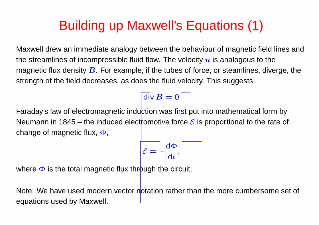
Maxwell drew an immediate analogy between the behaviour of magnetic field lines andthe streamlines of incompressible fluid flow. The velocity u is analogous to themagnetic flux density B. For example, if the tubes of force, or steamlines, diverge, thestrength of the field decreases, as does the fluid velocity. This suggests

div B = 0

Faraday’s law of electromagnetic induction was first put into mathematical form byNeumann in 1845 – the induced electromotive force E is proportional to the rate ofchange of magnetic flux, Φ,

E = −dΦ

dt,

where Φ is the total magnetic flux through the circuit.

Note: We have used modern vector notation rather than the more cumbersome set ofequations used by Maxwell.

21

Building up Maxwell’s Equations (2)

Since E =∫

E · ds and Φ =∫

B · dS, Stokes’ theorem leads directly to

curlE = −∂B

∂t.

Since Ienclosed =∫

J · dS, Stokes’ theorem converts Ampere’s law∫C

H · ds = Ienclosed,

into

curlH = J .

22

Building up Maxwell’s Equations (2)

Since E =∫

E · ds and Φ =∫

B · dS, Stokes’ theorem leads directly to

curlE = −∂B

∂t.

Since Ienclosed =∫

J · dS, Stokes’ theorem converts Ampere’s law∫C

H · ds = Ienclosed,

into

curlH = J .

Finally, from Poisson’s equation, he knew that

div E =ρe

ǫ0.

in free space.

23

The Primitive Form of Maxwell’s Equations

These results form the primitive and incomplete set of Maxwell’s equations.

curlE = −∂B

∂t

curlH = J

div ǫ0E = ρe

div B = 0

Maxwell still lacked a physical model for the phenomena of electromagnetism. Hedeveloped his solution in 1861-2 in a remarkable series of papers entitled On physicallines of force.

Since his earlier work on the analogy between u and B, he had become convinced thatmagnetism was essentially rotational in nature. He began with the model of a rotatingvortex tube as an analogue for a tube of magnetic flux.

24

Maxwellian Vortices

A rotating vortex tube was taken as an analogue for a tube of magnetic flux.

If left on their own, magnetic field lines expand apart, exactly as occurs in the case of avortex tube if the rotational centrifugal forces are not balanced. The rotational kineticenergy of the vortices as ∫

vρu 2 dv,

where ρ is the density of the fluid and u its rotational velocity. This is similar to theexpression for the energy of a magnetic field,

∫v(B

2/2µ0) dv. Thus, again u isanalogous to B.

Maxwell postulated that everywhere the local magnetic field strength should beproportional to the angular velocity of the vortex, so that the angular momentum vectoris parallel to the axis of the vortex, and so parallel to the magnetic field direction.

25

Maxwellian Vortex Tubes

Maxwell began with a model in whichthe whole of space was filled with vortextubes. However, friction betweenneighbouring vortices would cause themto dissipate.

Maxwell therefore inserted‘idler-wheels’, or ‘ball-bearings’,between the vortices so that they couldall rotate in the same direction withoutfriction.

26

Maxwellian Vortex Tubes

Maxwell’s original picture of thevortices represented by rotatinghexagons. The diagram shows acurrent flowing through vortices.

He then identified the ‘idler-wheels’ withelectric particles which, if they were freeto move, would carry an electric current.In conductors, these electric particles arefree to move, whereas in insulators,including free space, they cannot moveand so cannot carry an electric current.

Remarkably, this model could explain allknown phenomena of electromagnetism.

27

Electromagnetism and Vortices

The magnetic field of a current carryingwire.

The magnetic field distribution in thepresence of a current sheet.

Electromagnetic induction

28

The Displacement Current (1)

Maxwell next considered how insulators store electrical energy. In insulators, themedium is elastic so that the electric particles can be displaced from their equilibriumpositions by the action of an electric field. The electrostatic energy in the medium wasidentified with the elastic potential energy associated with the displacement of theelectric particles. This had two key consequences:

• When the electric field applied to a medium is varying, there are small changes inthe positions of the electric particles in the insulating medium or vacuum, and sothere are small currents associated with this elastic motion. There is a currentassociated with the displacement of the electric particles from their equilibriumpositions which Maxwell called the displacement current.

29

The Displacement Current (2)

• Because the medium is elastic, the speed at which disturbances can bepropagated through the insulator, or vacuum, can be calculated. The calculation isstraightforward.

The displacement of the electric particles is assumed to be proportional to the electricfield strength

r = αE.

When the strength of the field varies, the charges move causing a displacementcurrent. If Nq is the number density of electric particles and q their charge, thedisplacement current density is

Jd = qNqr = qNqαE = βE.

30

The Displacement Current (3)

This displacement current density should be included in the equation for curl H :

curlH = J + Jd = J + βE.

α and β are unknown constants to be found from the electric properties of the medium.Assuming there are no currents, J = 0, the speed of propagation of a disturbancethrough the medium is the solution of the equations

curlH = βE,

curlE = −B.

We seek wave solutions of the form ei(k·r−ωt) and then, using the standard procedure,we find a dispersion relation

k × (k × H) = −ω2βµ0H.

For transverse waves, this reduces to

c2 = 1/βµ0

31

The Determination of β

The energy density stored in the dielectric is the work done per unit volume indisplacing the electric particles a distance r,

Workdone =

∫F · dr =

∫NqqE · dr.

But

r = αE and hence dr = αdE.

Therefore, the work done is∫ E

0NqqαE dE = 1

2αNqqE2 = 12βE2.

But the electrostatic energy density in the dielectric is 12D · E = 1

2ǫ0E2. Thereforeβ = ǫ0. Inserting this value into the expression for the speed of the waves,

c = (µ0ǫ0)−1/2

32

Light as Electromagnetic Waves

Maxwell inserted the best available values for the electrostatic and magnetostaticconstants into the expression for c and found, to his amazement, that it turned out to bethe speed of light, within a few percent. In his own words:

‘we can scarcely avoid the inference that light consists in the transversemodulations of the same medium which is the cause of electric and magneticphenomena’.

‘I do not bring it forward as a mode of connection existing in Nature....

It is however a mode of connection which is mechanically conceivable and itserves to bring out the actual mechanical connections between knownelectromagnetic phenomena.’

33

A Dynamical Theory of theElectromagnetic Field (1865)

In 1864, Maxwell developed the whole theory on a much more abstract basis withoutany special assumptions about the nature of the medium through whichelectromagnetic phenomena are propagated. To quote Whittaker:

‘In this, the architecture of his system was displayed, stripped of the scaffoldingby aid of which it had been first erected’.

Maxwell’s own view of the significance of this paper is revealed in what Everitt calls ‘arare moment of unveiled exuberance’ in a letter to his cousin Charles Cay:

‘I have also a paper afloat, containing an electromagnetic theory of light,which, till I am convinced to the contrary, I hold to be great guns’.

34

Maxwell’s Equations in their Final Form (1)

In Maxwell’s great papers, eight equations were involved. The standard form of theequations was introduced by Heaviside and Hertz in the 1880s.

curlE = −∂B

∂t,

curlH = J +∂D

∂t,

div D = ρe,

div B = 0.

The inclusion of the displacement current ∂D/∂t resolves a problem with the equationof continuity in electromagnetism. Taking the divergence of the second equation,

div(curlH) = div J +∂

∂t(div D) = 0

35

Maxwell’s Equations in their Final Form (2)

Since divD = ρe,

div J +∂ρe

∂t= 0,

the continuity equation for conservation of electric charge in electrostatics.

Notes:

1. Maxwell’s discovery gave real physical content to the wave theory of light.

2. Poincare: In his experience, all Frenchmen were oppressed by a ‘feeling ofdiscomfort, even of distress’ at their first encounter with the works of Maxwell.

3. When Maxwell became the first Cavendish Professor in 1871, he devotedconsiderable effort to the precise determination of the ratio of the electrostatic andelectromagnetic units.

36

Hertz’s Experiments (1)

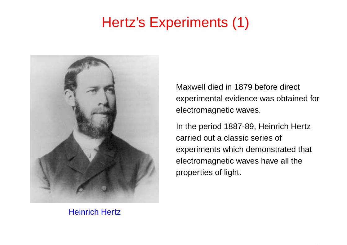
Heinrich Hertz

Maxwell died in 1879 before directexperimental evidence was obtained forelectromagnetic waves.

In the period 1887-89, Heinrich Hertzcarried out a classic series ofexperiments which demonstrated thatelectromagnetic waves have all theproperties of light.

37

Hertz’s Experiments (2)

This apparatus is on show in theDeutsches Museum in Munich.

He found standing waves as thedetector was moved along the linebetween the emitter and theconducting sheet. The frequency ofthe waves was found from theresonant frequency of the receivingloop, ω = 2πν = (LC)−1/2, where L

and C are the inductance andcapacitance of the detector. Thewavelength of the waves was twice thedistance between the minima of thestanding waves and c = νλ. Theresult was precisely the speed of light.

38

Hertz and the Photoelectric Effect

Hertz went on to demonstrate that the electromagnetic waves exhibited all theproperties of light waves. In his great book Electric Waves (1893), the chapter headingsinclude:

Rectilinear Propagation, Polarisation, Reflection, Refraction.

To demonstrate refraction he constructed a prism weighing 12 cwt out of ‘so-called hardpitch, a material like asphalt’.

Ironically, in the same set of experiments which completely established Maxwell’stheory, he also discovered the photoelectric effect. This effect was central to Einstein’sdemonstration that light has particle as well as wave properties. It led directly to thedevelopment of the quantum theory of matter and radiation.

39

Why is Maxwell not Better Known?

Maxwell was very modest about his achievements. In his 1870 Presidential Address tothe BAAS reviewing advances in physics and electromagnetism, he reviewed all theother theories but not his own, merely referring to:

‘Another theory of electromagnetism which I prefer.’

Freeman Dyson (1999)

‘The moral of this story is that modesty is not always a virtue.’

40

Freeman Dyson on Maxwell

‘Maxwell’s theory becomes simple and intelligible only when you give up thinking interms of mechanical models. Instead of thinking of mechanical objects as primary andelectromagnetic stresses as secondary consequences, you must think of theelectromagnetic field as primary and mechanical forces as secondary. The idea that theprimary constituents of the universe are fields did not come easily to the physicists ofMaxwell’s generation. Fields are an abstract concept, far removed from the familiarworld of things and forces. The field equations of Maxwell are partial differentialequations. They cannot be expressed in simple words like Newton’s law of motion,force equals mass times acceleration.

Maxwell’s theory had to wait for the next generation of physicists, Hertz and Lorentzand Einstein, to reveal its power and clarify its concepts. The next generation grew upwith Maxwell’s equations and was at home with a Universe built out of fields. Theprimacy of fields was as natural to Einstein as the primacy of mechanical structureshad been for Maxwell.’

41