The Origins of Ethnolinguistic Diversity: Theory and Evidence

Stelios Michalopoulos�

July 2, 2007

Abstract

This research examines theoretically and empirically the economic origins of cultural di-versity and sheds new light on the emergence of ethnolinguistic fractionalization. The studyargues that di¤erences in the productive activities across regions led to the emergence ofregion speci�c human capital. Among regions characterized by dissimilar productive en-dowments, population mixing was limited leading to the formation of localized ethnicitiesand languages, producing a wider ethnolinguistic spectrum. Using new detailed data onthe global distribution of land quality, the empirical analysis conducted in a cross coun-try as well as cross-region framework, reveals that variation in land quality contributedsigni�cantly to the emergence and persistence of ethnolinguistic diversity. The empiricalresults also document the impact of European colonization on the ethnic diversity of thecolonized world both through the drawing of the borders and the active manipulation of theunderlying ethnicities. This research contributes to an understanding of the emergence andthe distribution of languages and ethnicities and constitutes a �rst step towards compre-hending the natural, i.e. geographically driven, and arti�cial, i.e. man-made, componentsof contemporary ethnolinguistic diversity.Keywords: Ethnolinguistic Diversity, Geography, Technological Progress, Population Mix-ing, ColonizationJEL classi�cation Numbers: O11, O15, O33, O40, J20, J24.

�I am indebted to Oded Galor for his constant advice and mentorship. Comments from Andrew Foster, IoannaGrypari, Peter Howitt, Nippe Lagerlof, Ashley Lester, Ross Levine, Glenn Loury, Ignacio Palacios-Huerta andDavid Weil as well as seminar participants at Brown University were very helpful. Lynn Carlsson�s ArcGisexpertise proved of invaluable assistance.

1

1 Introduction

This study provides a theoretical and empirical framework for understanding the economic

origins of ethnic diversity. The formation of ethnic diversity has been a long standing topic

of research in the realm of social sciences. A rich literature in the �elds of political science,

psychology, sociology, anthropology and history attests to it, see Hale (2004). However, the

economic origins of ethnic diversity are poorly understood both from an empirical and a the-

oretical point of view, limiting the conclusions that may be drawn from the existing intensive

discourse across disciplines. A similar concern also applies to the large and growing literature

within economics which has focused on the relationship between ethnolinguistic diversity and

economic outcomes. Consequently, identifying the foundations of ethnic diversity will deci-

sively improve upon the interpretation of the existing literature. In particular, uncovering the

forces behind the emergence of di¤erential ethnic traits will have important implications for

understanding comparative economic development today.

Providing a theory of how ethnic identity, cultural practises, religion and language are

constructed is beyond the scope of this research. However, given that such elements of human

behavior have emerged universally in all societies the puzzle remains as to why some places

exhibit higher or lower levels of cultural diversity. Exploring the rise of ethnic diversity and

identifying its underlying components is the goal of this research.

The key �nding of this study is that diversity in land qualities across regions contributed

signi�cantly to the emergence and persistence of ethnic diversity. The empirical results, in

particular show that contemporary ethnic diversity displays a natural component and a man-

made one. The natural component is driven by the diversity of land quality across regions,

whereas the man-made part re�ects the idiosyncratic state histories of each country, including

the colonial experience and the emergence of modern states among other things.

There are three elements that form the basis of the theory. The �rst is that variation in

the set of optimal productive activities across regions, generated by the underlying variation

in land qualities, gave rise to region speci�c human capital. These di¤erences in region speci�c

human capital constituted a barrier to population mixing. Subsequently, the extent to which

localities overlapped regarding their productive characteristics determined how easy was for the

local populations to transfer their region speci�c human capital. Distribution of land qualities

conducive to regionally distinct sets of productive activities e¤ectively hindered population

mobility between places. On the other hand, places exhibiting more homogeneous productive

structures would facilitate mixing of the local populations resulting in the formation of common

2

ethnolinguistic behavior.

Over time site speci�c productivity shocks generated incentives to relocate. According

to the theory it is the interaction of these two elements, the easiness to transfer regional human

capital and the incentive to change locality, induced by variation in the regional productivity

shocks, that gave rise to di¤erences in ethnic diversity both within and across countries.

As already mentioned the formation of common cultural and ethnolinguistic traits for

a pair of regions is positively related to the intensity of population mixing within this pair.

Such formulation derives from the observation that a region experiencing infrequent population

exchanges is bound to give rise to distinct ethnolinguistic traits as cultural drift may dominate

the evolution of the characteristics of such places. By not imposing a binary relationship in

the ethnic similarity between two regions, the analysis may also be applied to understanding

ethnic or linguistic distance, with higher intensity of population mixing leading to lower ethnic

distance.1

Ethnicities and languages were formed in a stage of development when land was the

single most important factor of production. The theory, thus, predicts that ethnic diversity

should be prominent as long as land is the major input in the production process. On the other

hand, during an era when general human capital,2 rather than region speci�c ethnic capital, is

the individual input to the production process, ethnic and linguistic markers would gradually

become less salient since population mixing would be more frequent.3

In this respect the proposed theory bridges the divide in the literature regarding the

formation of ethnicities, by identifying the economic mechanism at work. There are two main

strands of thought within. The primordial one quali�es ethnic groups as deeply rooted clearly

drawn entities, Geertz (1967), whereas the constructivists or instrumentalists, Barth (1969),

highlight the contingent and situational character of ethnicity. In the current framework, it is

the heterogeneity in land�s productive traits that gives rise initially to relatively stable ethnic

diversity, an element of primordialism. However, as the process of development renders land

increasingly unimportant then ethnic identity is bound to become less attached to a certain set

of region speci�c skills and, thus, more situational and ambiguous in character.4

1Note that this statement applies in the long run. In the short run migration movements may increasediversity in the receiving place, see Williamson (2006).

2This obtains under the following assumptions. First, there is no assortative mating according to ethnicity,second all ethnicities in the non land-intensive stage of development have the same opportunities to acquirehuman capital and the institutions in place do not generate a systemic bias against any of them.

3For a discussion of the salience of ethnic identity on the eruption of civil con�ict see Esteban and Ray (2007).4 In other words, as the importance of region speci�c knowledge diminishes, ethnicity gradually transforms

into a consumption good.

3

The model developed employs a stochastic, one sector, two-region overlapping genera-

tions framework. Land, labor and region speci�c technology are employed in each regional

production function. The technology in every area develops over time through learning by

doing, and is available to the indigenous population. People in the beginning of each period

compare the potential income of their place of origin to that in case of moving and act ac-

cordingly. The incentive to move stems from the di¤erential impact of temporary regional

productivity shocks. Transferring region speci�c know-how across places, however, is costly

in the sense that it may not be applicable to the receiving place. In fact, this cost increases

in the heterogeneity of productive activities between places. Consequently, conditional on the

productivity shocks, regions with larger overlap in their productive characteristics would ex-

perience more frequent population exchanges. Similarly, pairs of areas characterized by larger

regional productivity �uctuations would display consistently more intense population mixing,

ceteris paribus.

The proposed framework may also be used to understand both long-range migratory

movements like the spread of the �rst agriculturalists and herders following the Neolithic Rev-

olution as well as migratory patterns within shorter ranges. The historical evidence in section

2, centers on both the cause and e¤ect of long range and short range population movements

on linguistic spreads.

In the empirical section the regional heterogeneity in productive structures, which is

the focus of the theory, is proxied using detailed regional data on the distribution of land

quality for agriculture for the whole world. The econometric analysis is conducted in a cross-

region as well as a cross country framework. For the cross-region regressions I arbitrarily

divide the world into geographical entities of a given size and consistent with the theory I

�nd that the number of languages spoken in these regions is systematically related to the

underlying variation in land quality. Regions characterized by a wider spectrum of land qualities

give rise and support larger linguistic fragmentation. Including continental and country �xed

e¤ects, e¤ectively taking into account the idiosyncratic state and continental histories, the

�ndings remain robust. Moving into a cross-country framework the proposed hypothesis is

also validated. Countries characterized by more heterogeneous land qualities, exhibit higher

ethnolinguistic fractionalization. This highlights the fundamental role that the spectrum of

regional land qualities has played in the formation of more or less culturally diverse societies.

Testing alternative hypotheses regarding the formation of ethnolinguistic diversity, fo-

cusing on di¤erential historical paths like the timing of the emergence of modern states, the

4

population in 1500 as a proxy for early economic development, and additional geographical

characteristics like elevation and distance from the sea among other features, the qualitative

predictions remain intact. Interestingly, the identi�ed strong negative impact of the distance

from the equator on ethnic diversity is consistent with the prediction that places experiencing

persistent productivity shocks are conducive to low ethnic diversity. Note that distance from

the equator correlates with seasonality. This emphasizes the economic basis of the origins of

cultural diversity.

Historical accidents have in�uenced fractionalization outcomes. The European coloniza-

tion after the 15th century, for example, is an obvious candidate. Analyzing the role of the

colonizers in a¤ecting the ethnolinguistic diversity of the colonized countries, reveals important

patterns. The evidence is suggestive of the historically documented arbitrariness of border

drawing, see Englebert et al. (2002). In particular, the results show that the way borders

were drawn, generated a spectrum of land qualities which was conducive to higher ethnolin-

guistic diversity. However, colonizers did not only a¤ect the geographically determined level

of fractionalization. As a consequence of the introduction of their own ethnicity and the ac-

tive interfering with the local populations, they generated arti�cial fractionalization, that is a

component of ethnolinguistic diversity which was not an outcome of the underlying geography.

This decomposition of observed fractionalization into natural, i.e. driven by the distribution of

land qualities, and man-made components, o¤ers new insights regarding the origins of cultural

diversity, highlighting the role of variation in land quality and colonial history in particular.

By identifying the role of the European colonizers in a¤ecting both the natural and

arti�cial elements of ethnolinguistic diversity this research adds to the literature on the impact

of European colonization on the indigenous economies (La Porta et al. (1999), Acemoglu,

Johnson and Robinson (2001)). The �ndings are also closely related to a recent study by

Alesina et al. (2006) in which new measures of state arti�ciality are proposed. Man-made

fractionalization, measured by the fraction of ethnolinguistic diversity not explained by the

underlying distribution of land quality, increases signi�cantly the probability of being included

in the top 13 most arti�cial states that the authors provide. Naturally, it remains to be seen

whether such relationship is relevant to the whole dataset or is only a feature of the identi�ed

countries.

This study is also directly related to the strand of literature that concerns the rela-

tionship between ethnolinguistic fractionalization and countries� economic performance, see

Easterly and Levine (1997), Fearon and Latin (2003) and Alesina et. al. (2003) among others.

5

The theoretical and empirical thesis shows that ethnic diversity is driven by the distribution of

land quality within a country. At the same time the empirical analysis shows that the divergent

state histories of existing countries, evident in the presence or absence of colonization as well

as in the levels of early economic development, have in�uenced signi�cantly the contempo-

rary ethnolinguistic endowment. Consequently, the documented negative relationship between

ethnolinguistic fractionalization and economic outcomes may re�ect the direct e¤ect of state

history rather than a true e¤ect of ethnic diversity. Thus, further research on the causal impact

of ethnic diversity on comparative economic development today is warranted.5

Another line of research to which the �ndings are relevant is a recent study by Spolaore

and Wacziarg (2006). The authors document empirically the e¤ect of genetic distance, a

measure associated with the time elapsed since two populations� last common ancestors, on

the pairwise income di¤erences between countries. Larger genetic distance inversely a¤ects the

adoption of technology. In the proposed framework population mixing between two regions,

may directly reduce genetic distance. Thus, the latter is endogenous to both the regional

productivity shocks and the transferability of region speci�c technology within the pair. As

a result, countries that are relatively dissimilar in the distribution of productive possibilities,

will be populated by people displaying larger genetic distance, ceteris paribus. Consequently,

the uneven di¤usion of development across countries may be an outcome of the di¤erences in

country speci�c human capital rather than genetic distance itself. It would be interesting to

replicate their empirical analysis introducing the pair-wise country distances of the distribution

of land quality. An inclusion of such control is bound to partially account for the documented

signi�cant e¤ect of genetic distance on pair-wise income comparisons.

The results could be also used to understand the di¤usion of technology not only across

but also within countries. Technology would di¤use more quickly in more homogeneous coun-

tries, land quality wise, whereas in relatively heterogeneous ones, and according to the theory

and evidence more culturally diverse, the di¤usion would be less rapid leading to the emergence

of inequality among ethnic groups. This would obtain because of the di¤erential complemen-

tarity between a new technology and the preexisting variation in ethnic speci�c human capital

re�ecting the variation in regional land qualities. Intuitively speaking, herders unlike farmers

would be less likely to adopt a new technology speci�c to farming.

This research sheds new light on the emergence and the distribution of languages and

ethnicities and constitutes a �rst step within economics towards the understanding of natural

5Michalopoulos (2007b) uses the proposed framework to uncover the causal impact of ethnolinguistic diversityon the economic performance across countries looking on a variety of economic indicators.

6

and man-made components of ethnic diversity. This study is a stepping stone for further

research. Equipped with a more substantive understanding of the origins and determinants

of ethnolinguistic diversity, new ways of addressing long standing important questions among

development and growth economists may be o¤ered. These range from the formation of states,

to the inequality across ethnic groups, to the e¤ect of ethnolinguistic diversity on the eruption

of civil wars, public good provision and economic outcomes in general.

The paper is organized as follows. In Section 2 (pre)historical evidence regarding the

occurrence of migrations and the spread of linguistic groups is brie�y reviewed. Section 3

presents the theory and its predictions. Section 4 discusses the data and covers the empirical

analysis conducted both in a cross-region and a cross-country framework, including the various

robustness checks and �nally focusing on the impact of the European colonizers on the observed

fractionalization outcomes. The last section concludes.

2 Evidence on Migrations and Language Spreads

The theory rests upon three fundamental building blocks: (i) population movements in�uence

the ethnolinguistic diversity of the places involved, leading eventually to a convergence in the

underlying traits (ii) migration of ethnic groups and languages occurs more often among places

with similar productive endowments (iii) regional productivity shocks generate the incentive

to relocate from one place to another.

Among linguists it has been long recognized the role of population mixing in producing

common linguistic elements between places. As Nichols (1997) points outs �almost all litera-

ture on language spreads6 focuses on either demographic expansion or migration as the basic

mechanism�. Both instances are a result of the movement of populations towards territories

previously unoccupied by their ancestors. In these new regions population mixing leads to

language shift (either to or from the immigrants�language). Also, languages long in contact

come to resemble each other in several dimensions like sound structure, lexicon, and grammar.

This resultant structural approximation is called convergence. To the extent that recurrent

contact between regional populations may occur through repetitive cross migrations (short-

term or long-term), the modeling of the emergence of common ethnolinguistic characteristics

as an increasing function of population mixing between places is justi�ed.

There are several examples showing that migrations have been occurring between places

6Nichols (1997) de�nes a spread zone as �an area of low density where a single language or family of languagesoccupies a large range�

7

of similar productive characteristics. Linguistic research has identi�ed several regions of the

world which are spread zones of languages, that is regions characterized by low linguistic diver-

sity. A common characteristic of such regions is the underlying homogeneity in the endowment

of land quality, as it is the case for the grasslands of central Eurasia. Generally, large spread

zones are associated with high latitudes where seasonality is evident and arid interiors, whereas

linguistic heterogeneity increases in the less seasonal climates, Nichols (1997). These distrib-

utional features highlight the role of variations in productivity shocks in shaping migration

movements and, ultimately, linguistic patterns.

Examples of groups that migrated along areas that were similar to their region of ori-

gin are Austronesians and speakers of Eskimoan languages who are coastally adapted peoples,

and accordingly they have spread along coasts rather than inland. Along similar lines, Bell-

wood (2001) argues that the spread zones of agriculturalists and their languages following

the Neolithic Revolution trace closely the distribution of land qualities that were relevant for

agricultural activities. In fact, the pattern of the languages�expansion, belonging to the Indo

European family, after the Neolithic revolution is embedded to the notion of �spread�and �fric-

tion�or �mosaic�zones. �Spread�regions were characterized by similar land qualities where

the early agriculturalists in the case Indo-European languages7, or nomad pastoralists in the

case of the Turkic and Mongolian languages (these belong to the Altaic language family) could

easily apply their own speci�c knowledge and friction zones were places less conducive to either

activity. In such places the populations maintained their distinct ethnolinguistic behavior. Ex-

amples of the latter include regions like Melanesia, Western and Northern Europe and Northern

India, see Renfrew (2000) for a comprehensive review. This implies that early agriculturalists

and pastoralists, perhaps not surprisingly, targeted and expanded at areas where their speci�c

knowledge would best apply, homogenizing them linguistically. If this process of language shift

occurred through replacement of the local populations or by extensive intermarrying is yet an

open question.

Other relatively more recent examples of ethnic groups that consistently migrated to

places where they could utilize their ethnic human capital, include the Greeks and the Jews,

among others who belong to the historic trade diasporas, Cushin (1984). It is in this case the

knowledge of how to conduct commerce that allowed these groups to spread in areas where

merchandising was both possible and pro�table. Botticini and Eckstein (2006), for example,

document the religiously driven transformation of the Jewish ethnic human capital towards

7Gray and Atkinson (2003) produce evidence showing that IndoEuropean languages expanded with the spreadof agriculture from Anatolia around 8,000�9,500 years BP.

8

literacy and the resulting expansion.

Generally, according to the theory migratory movements should be relatively more fre-

quent among ethnic groups whose knowledge is less attached to speci�c land attributes, as in

the case of trade diasporas. Should the ethnic knowledge be region speci�c, though, then such

groups would disperse in places that are similar to the place of origin regarding the underlying

productive activities, minimizing, thus, erosion of their speci�c human capital.

Regarding the e¤ect of di¤erential climatic shocks in generating movements of people

evidence suggests that this was indeed an important factor.8 For example, as Nichols (1997)

suggests, at least since the advent of the Little Ice Age in the late middle ages highland

economies have been precarious, whereas the lowlands, with their longer growing seasons,

were relatively prosperous o¤ering winter employment for the essentially transhumant male

population of the highlands. This caused lowland dialects to spread uphill. Prior to the global

cooling, however, lowlands were dry and uplands moist and warm. Under these conditions, with

highlands being relatively more economically secure, upland dialects spread downhill, through

a similar process. The linguistic patterns present in regions like central Caucasus (Nichols

1997b) and the highland spread of Quechua fall in this category.

The linguistic and (pre)historical evidence for the spread of peoples and languages provide

ample support to the building blocks of the theory presented below.

3 The Basic Structure of the Model

Consider an overlapping-generations economy in which economic activity extends over in�nite

discrete time. Each individual lives two periods and bears exactly one child in the second period

of her life, i.e. population is �xed. In every period the economy produces a single homogeneous

good using land, labor and region speci�c technology as inputs in the production process. The

supply of land is exogenous and �xed over time. In fact, there are two regions in the economy

i and j. The supply of labor in each place is determined by the evolution of the region speci�c

know-how, its transferability between the places and the state of the temporary idiosyncratic

productivity shock relative to the other region.

8The independent role of regional climatic �uctuations in generating di¤erential timing of the transition toagriculture has been proposed by Ashraf and Michalopoulos (2006).

9

3.1 Production of Final Output

Production in each area displays constant-returns-to-scale with respect to land and labor. The

output produced at time t in region r; Y rt ; is

Y rt = (zrt hrt ) (L

rt )� (mrXr)1��; � 2 (0; 1); r 2 fi; jg (1)

where zrt is the productivity shock in period t in region r; hrt is the level of knowledge in period

t relevant to region r which evolves over time through learning by doing - it may be interpreted

as region speci�c human capital - Lrt is the total labor employed in period t in region r; mr

represents the land quality of region r and Xr is the size of land used in production in every

period in region r (which for simplicity is normalized to 1 for all r).

Suppose that there are no property rights over land.9 The return to land in every period

is therefore zero, and the wage rate in period t is equal to the output per worker produced at

time t; yrt :

yrt = (zrt hrt ) (m

r=Lrt )1�� (2)

3.2 Preferences

In every period a generation, which consists of a continuum of individuals of measure L, is

born. Speci�cally, an agent born in period t; gives birth at the beginning of period t + 1 in

the region where she works at that period. People, within as well as across generations, are

identical in their preferences and their ability in utilizing the technology of the region they

are born to. Individuals live for two periods. In the �rst period, they are economically idle,

passively accumulating the speci�c know-how of the place they are born to. In the second

period they supply inelastically their unit of labor and consume the earnings.

Individuals�preferences are de�ned over consumption in the second period of their lives,

ct+1.10 The preferences of an individual n born in period t are, thus, represented by the utility

function,

ut;n = u�ct;nt+1

�(3)

9The modeling of the production side is based upon two simplifying assumptions. First, capital is not aninput in the production function, and second the return to land is zero. Allowing for capital accumulation andprivate property rights over land would complicate the model to the point of intractability, but would not a¤ectthe qualitative results. Speci�cally, if property rights were preassigned to the indigenous then the rental price ofland would adjust as a result of the demand from migrants. Alternatively, property rights could be endogenizedin a con�ict model sharing the same primitive characteristics as the current set up leading to qualitative similarpredictions.10Allowing both for endogenous fertility and intergenerational altruism the predictions would not be reversed.

10

where ct;nt+1 is the consumption of a member n of generation t in period t+1. The utility

function is strongly monotone and strictly quasi-concave.

3.3 Accumulation of region speci�c technology

The level of regional technology available to the indigenous population at time t in region r

advances as a result of learning by doing.

hrt+1 = (hrt ) ; r 2 fi; jg

with hr0 = 1; hrr > 0 and hrthrt < 0; that is, the level of regional know-how in any period

is a monotonically non-decreasing concave function of the level of know-how in the preceding

period. Since both region speci�c technologies start from the same initial level and follow the

same law of motion, the technology available to the indigenous in each region is identical in

every period. That is,

hjt = hit 8 t � 0 (4)

Di¤erences in the accumulation rate of region speci�c technology would not alter the

predictions of the model. As it will become apparent it would in principle make people of

the region enjoying a higher technological growth rate less willing to move, ceteris paribus.

Furthermore, it�s not a priori clear which places should enjoy higher technological accumulation

rates. The literature has stressed both the role of pure population density, which is proportional

to the productivity of the land, see Galor and Weil (2000), and the �necessity as the mother

of invention�in promoting technological progress. For the latter see Boserup (1965).

3.4 Transferring region speci�c technology across places

As adults, individuals may move freely from one region to another.11 However, this comes at

a cost arising from di¤erences in territory-speci�c human capital. In particular, since the level

of technology, hrt ; is region r speci�c, relocation renders obsolete part of the knowledge that

the individual may apply as a worker in the receiving place. This erosion increases as places

become increasingly di¤erent in the feasible and/or optimal set of productive activities.

11 Including additional costs associated with migration, either as a result of time expended on relocating or inthe form of a transfer to the indigenous in the receiving area would not change the results. It would, however,add an additional dimension along which places might di¤er.

11

The following equation captures how the know-how of the region of origin is converted

into units of know-how relevant to the receiving place:

krt = (hqt )1�" 8 r; q 2 fi; jg; r 6= q;

0 � " � 1; hqt � 1(5)

where krt are the units of knowledge that a migrant will be able to apply should she move to

region r and " captures the degree of erosion within regional pairs. Those characterized by more

heterogeneous endowments score higher along this dimension. Note that within a regional pair

erosion of region-speci�c knowledge is symmetric, thus it is quantitatively identical irrespective

of the direction of the migration.

The properties of transferring region-speci�c technology across places, follow directly by

di¤erentiating (5):

1. The migrant�s level of know-how relevant to the receiving place decreases in the level of

erosion between the regions, @krt

@" < 0 8 r 2 fi; jg

2. The migrant�s level of know-how relevant to the receiving place increases in the level of

know-how of the place of origin, @krt

@hqt> 0;8 r; q 2 fi; jg; r 6= q:

2. There exist diminishing returns to the transferability of the know-how of the place of

origin, @2krt@2hqt

< 0; 8 r; q 2 fi; jg; r 6= q: This captures the fact that the accumulation

of technology becomes increasingly region speci�c and, as a result, less useful in case of

migration.12

3. Lastly, the transferability of region-speci�c knowledge decreases with the level of erosion,@2krt@hqt@"

< 0; 8 r; q 2 fi; jg; r 6= q: In other words, an additional unit of domestic know-how

is less applicable to the receiving region in pairs characterized by higher erosion.

Taking into account (4) and the preceding discussion, it follows that the indigenous

population of region r; that is individuals who work in the same region they are born to, have

higher level of know-how compared to that of the migrants during the period the migrants

arrive, that is the output per worker is higher for the indigenous population.13 Speci�cally,

using (2)12Such diminishing returns could be conceived as an outcome of increasing specialization in the set of activities

relevant for each region. At any given level of heterogeneity within a pair of regions, further specialization inthe respective activities diminishes the transferability of the additional know-how.13 It is useful to note that migrants�o¤spring have the same level of region speci�c human capital as the o¤spring

of non-migrants. Gradual accumulation of the region speci�c technology for the o¤spring of immigrants would

12

yrt = (zrt hrt ) (m

r=Lrt )1��

yq!rt = (zrt krt ) (m

r=Lrt )1��

(6)

8 r; q 2 fi; jg; r 6= q:

where yrt is the output per indigenous worker of region r and yq!rt is the output per

migrant-worker from region q working in region r:

3.5 De�ning Common Ethnicity

A probabilistic framework regarding the formation of shared ethnolinguistic elements is adopted.

Particularly, it is conjectured that the probability that individuals from regions i and j will

share common traits increases in the intensity of population mixing between the two regions

over time.14 As individuals cross-migrate, they add their cultural traits from the place of origin

to the cultural pool of the indigenous population. This addition may be an outcome of the pure

interaction in everyday activities between the locals and the contemporary immigrants or may

take the form of intermarrying. Although we do not explicitly model the household formation

decision the probability of mixed households would increase in the intensity of cross migration.

Should this process occur incessantly over time, then the respective regions would share an

increasingly larger set of common practices. On the other hand, pairs of regions characterized

by few past cross�migrations would evolve to exhibit distinct ethnolinguistic characteristics.

Formally, let fT denote the probability that places, i and j, observed in period T will

exhibit common ethnolinguistic elements.

fT =

TPt=1

It

T(7)

where It is an indicator function that takes the value of 1 if migration occurs in period t

between regions i and j; irrespective of the direction; and 0 otherwise. Such formulation could

alternatively be interpreted as an inverse measure of ethnic distance between the two regions.

As already mentioned since this relationship applies in the long-run, T should be thought as

relatively large. According to this de�nition pairs of places whose populations never mixed

not alter the results. It could, however, create selection into reverse migration of the people whose ancestorswere immigrants.14Assuming either perfect initial ethnolinguistic heterogeneity or perfect homogeneity across regions does not

a¤ect the pattern of ethnolinguistic assimilation. Should the latter be the case, then cultural practices are formedregionally as time evolves due to cultural drift, Boyd and Richardson (1985).

13

until period T would have zero probability of sharing common ethnic traits, or alternatively

put, maximal ethnolinguistic distance. Alternative speci�cations of (7) could accommodate a

potential �founder�e¤ect in case that earlier migrations have a larger impact than later ones

in the formation of common ethnicity. Also, including both the occurrence and the actual size

of migration in every period would reinforce the qualitative predictions.

Variations in the intensity of population mixing between regions are according to the

theory the main determinant of cultural diversity across places. The analysis below establishes

how this intensity varies according to the transferability of regional human capital.

3.6 Labor Allocation Across Regions

Since the utility of members of generation t depends only on their consumption as adults, utility

maximization is equivalent to maximizing lifetime income. In the beginning of every period t

productivity shocks, zrt ; which last for one period, are realized in each region. Adult individuals

observe the realization of the shock15 and decide whether or not to migrate by comparing the

respective incomes in (6).16 Erosion of region-speci�c technology decreases potential income in

case of relocation, whereas a relatively higher productivity shock in the host area acts as an

incentive to the prospective migrant. This is the fundamental trade-o¤ created by the forces

in the environment.

Consequently, in period t after the realization of regional productivity shocks and before

any migration movement, individuals in each region compare the potential income of either

migrating or staying in the region of origin given the ratio of the regional population densities

bequeathed from period t � 1: Let f�tgTt=0 denote the sequence of the ratio of productivityshocks of region i relative to region j, that is �t =

zitzjt: It follows that �t > 0 and �t T 1 iff

zit T zjt . Using (6) and substituting Lit; L

jt with the respective values of the preceding period,

individuals from region i have an incentive to migrate to region j in the beginning of period t

iff ;

yi!jt > yit ) �t <�hit��" mj

mi

Lit�1

Ljt�1

!1��(8)

15The analysis abstracts from imperfect information regarding the size of the regional productivity shocks.16Migration in this framework lasts for at least one generation. It would be straightforward to incorporate

short term migration by allowing for more subsequent productivity shocks per generation per region. Accountingfor seasonality in the climatic �uctuations, would strengthen the theoretical predictions. Conditional on thesimilarity of productive endowments, places characterized by higher seasonality would exhibit larger and morefrequent short-term migration movements.

14

Similarly, individuals from region j are willing to migrate to region i in the beginning of

period t iff :

yj!it > yjt ) �t >�hjt

�" mj

mi

Lit�1

Ljt�1

!1��(9)

It is obvious from (8) and (9) that the incentive to move depends on the relative size of

the regional productivity shocks, the level of the speci�c human capital of the region of origin,

the erosion that such a migration entails and the ratio of the population densities relative to

the ratio of land qualities.

Lemma 1 When individuals in one region strictly prefer to migrate then individuals in the

other region strictly prefer not to, i.e.,

yi!jt > yit ) yj!it < yjt

yj!it > yjt ) yi!jt < yit

Proof. It is straightforward to show that the right-hand side of (8) is always smaller than the

right-hand side of (9). They coincide when " = 0 or hjt = hjt = 1. �Given the absence of mobility barriers, as long as either of inequalities in Lemma 1 obtain

in the beginning of period t; population movement will be observed.

Let M i!jt ;M j!i

t denote the size of the population that migrates from region i to j and j

to i respectively in period t: The exact size of the realized migration is the one that makes the

marginal individual from the place of origin indi¤erent between moving and staying in the land

she was born. In particular, when in the beginning of the period t the incentive to migrate is

from region i to region j; then once migration, M i!jt ; has taken place, (8) should hold with

equality. Adding the size of the migration M i!jt in the receiving region, j; subtracting it from

the region of origin, i; and manipulating (8) the level of migration may be explicitly derived

M i!jt =

Lit�1 ���t�hit��� 1

1�� mi

mjLjt�1

1 +��t�hit��� 1

1�� mi

mj

(10)

Note that the numerator of (10) is always positive as a long as (8) holds in the beginning

of period t: Similar reasoning applies to deriving the size of the labor movement from region j

to region i: Speci�cally,

15

M j!it =

��t

�hjt

���� 11��

mi

mjLjt�1 � Lit�1

1 +

��t

�hjt

���� 11��

mi

mj

(11)

Again, note that the numerator in (11) is positive as long as (9) holds in the beginning

of period t:

3.6.1 Past Migrations

As it is evident from (10) and (11) the size of the migration movement in period t depends on

the level of regional population densities in the period t� 1. The following Lemma derives theratio of population densities in the beginning of every period t as a function of past migration

movements (if any).

Lemma 2 In the beginning of any period t; and before any labor movement occurs (if any) the

ratio of the regional population densities equalsLit�1Ljt�1

:17 There are two cases:

1 The last migration occurred in period s; 0 � s � t� 1 from region i to region j

Lit�1Ljt�1

= LisLjs=��s

�hi

s

��� 11�� mi

mjif M i!j

s > 0 (12)

2 The last migration occurred in period s; 0 � s � t� 1 from region j to region i

Lit�1Ljt�1

= LisLjs=

��s

�hj

s

���� 11��

mimj

if M j!is > 0 (13)

Proof. Depending on the direction of the last migration either (8) or (9) should hold with

equality when evaluated at the regional population densities after the occurrence of migration

in period, s. Solving for the ratio of regional population in period s; Lis

Ljs; completes the proof.�

Corollary 1 If last migration occurred in period s = 0, that is, it represented the initial

settlement of people across regions i and j; then the ratio of regional population densities in

period t� 1 equals:Lit�1

Ljt�1=Li0

Lj0= �0

mi

mj(14)

17The latter is identical to the ratio of population densities realized in the last occurrence of migration.

16

Proof. Follows from Lemma 2 and noting that (12) and (13) are identical evaluated at

hj

0 = hj

s = 1: �In Appendix A Lemma 4 establishes the properties of the size of the migration between

places given by (10) and (9).

3.7 The M iM j and M jM i loci

Given the de�nition of common ethnicity in (7) it is necessary to explore how the environment,

captured by the degree of erosion, the regional population densities, the contemporary level

of regional know-how and productivity shocks, determines the occurrence of migration in any

period t:

The M iM j locus is the geometric locus of all tuples�hit; �t;

Lit�1Ljt�1

; "

�such that the

marginal individual in region i is indi¤erent between moving or not, that is, yi!jt = yit:

M iM j �(

hit; �t;Lit�1

Ljt�1; "

!: yi!jt = yit

)Solving explicitly for the level of the relative productivity shock in period t; �tjM iMj , that

makes people in region i indi¤erent to moving i get:

yi!jt = yit ) �tjM iMj =

�Lit�1Ljt�1

mj

mi

�1�� �hit��" (15)

Similarly, M jM i is the geometric locus of all tuples�hjt ; �t;

Lit�1Ljt�1

; "

�such that the mar-

ginal individual in region j is indi¤erent between moving or not, that is, yj!it = yjt : In particular,

M jM i �(

hjt ; �t;Lit�1

Ljt�1; "

!: yj!it = yjt

)Thus, the level of the relative productivity shock in period t; �tjMjM i ; that makes people

from region j indi¤erent to moving is:

yj!it = yjt ) �tjMjM i =

Lit�1

Ljt�1

mj

mi

!1�� �hjt

�"(16)

As it is evident in (15) and (16) the ratio of the regional population densities from the last

period is important in determining the no-migration loci. From Lemma 2 the ratio of regional

population densities in period t� 1 may be expressed by either (12) or (13) depending on the

17

direction of the last movement across places in period s: The following lemma summarizes the

properties of the migration indi¤erence curves.

Lemma 3 Using Lemma 2 at any period t these are the properties of the non-migration loci

for each region

1. The M iM j locus@�t@hit

���M iMj

< 0 & @2�t@2hit

���M iMj

> 0

@�t@"

��M iMj < 0 & @2�t

@2"

���M iMj

> 0

@�t@�s

���M iMj

> 0 & @2�t@2�s

���M iMj

= 0

2. The M jM i locus@�t@hjt

���MjM i

> 0 & @2�t@2hjt

���MjM i

< 0

@�t@"

��MjM i > 0 & @2�t

@2"

���MjM i

> 0

@�t@�s

���MjM i

> 0 & @2�t@2�s

���MjM i

= 0

Proof. See Appendix A. �The pair of Figures below (1a; 1b) shows the e¤ect of the erosion, "; on the occurrence

of migration. As it follows from Lemma 3, conditional on the past that is on �s, hjs; and his;

the distance between the no-migration loci, M jM i andM iM j ; increases at the level of erosion.

This implies that given the contemporary productivity shock, �t; pairs of regions i and j

which are more dissimilar with respect to their productive structures experience infrequent

population mixing limiting the formation of common ethnolinguistic traits. Figure 1b is drawn

with a higher level of region speci�c technology than in 1a to exemplify the adverse e¤ect of the

accumulation of region speci�c human capital on migration outcomes. This obtains because

as people further specialize in their regions� speci�c productive activities the accumulating

knowledge becomes increasingly less transferable, hindering cross-migration. Note that in the

absence of erosion, i.e. at " = 0; regional knowledge is perfectly applicable across areas, as it

is e¤ectively general. In this case, the migration loci coincide and all it matters for migration

is the relative size of the current ratio of regional productivity shocks, �t; with respect to �s:

18

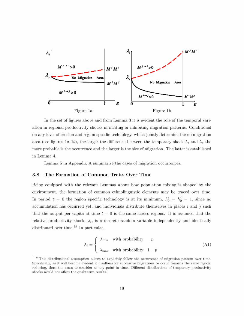
Figure 1a Figure 1b

In the set of �gures above and from Lemma 3 it is evident the role of the temporal vari-

ation in regional productivity shocks in inciting or inhibiting migration patterns. Conditional

on any level of erosion and region speci�c technology, which jointly determine the no migration

area (see �gures 1a; 1b), the larger the di¤erence between the temporary shock �t and �s the

more probable is the occurrence and the larger is the size of migration. The latter is established

in Lemma 4.

Lemma 5 in Appendix A summarize the cases of migration occurrences.

3.8 The Formation of Common Traits Over Time

Being equipped with the relevant Lemmas about how population mixing is shaped by the

environment, the formation of common ethnolinguistic elements may be traced over time.

In period t = 0 the region speci�c technology is at its minimum, hi0 = hj0 = 1, since no

accumulation has occurred yet, and individuals distribute themselves in places i and j such

that the output per capita at time t = 0 is the same across regions. It is assumed that the

relative productivity shock, �t; is a discrete random variable independently and identically

distributed over time.18 In particular,

�t =

8<:�min with probability p

�max with probability 1� p(A1)

18This distributional assumption allows to explicitly follow the occurrence of migration pattern over time.Speci�cally, as it will become evident it disallows for successive migrations to occur towards the same region,reducing, thus, the cases to consider at any point in time. Di¤erent distributions of temporary productivityshocks would not a¤ect the qualitative results.

19

with �min < �max: The following Proposition shows how erosion, "; the ratio of the

relative productivity shocks, �t=�s; and the level of regions speci�c technology determine the

probability that two regions will share common cultural elements.

Proposition 1 Under (A1)

1. The probability that regions i and j share common ethnolinguistic traits as observed in

period T; weakly decreases in the size of the erosion "

@fT (";�t; �s; hT )

@"� 0

2. The probability that regions i and j share common ethnolinguistic traits as observed in

period T; weakly increases in the variance of the regional productivity shock, �t;

@fT (�t; "; �s; hT )

@var (�t)> 0

3. The probability that regions i and j share common ethnolinguistic traits as observed in

period T; weakly decreases in the level of region speci�c human capital in period T; hT :

@fT (hT ; "; �t; �s)

@hT� 0

Proof. See Appendix A. �Proposition 1 underlines the key role geographic conditions play in the formation of

common ethnolinguistic traits. The adverse e¤ect of an increase in the region speci�c know-

how on the formation of common cultural elements stems from diminishing returns in the

transformation of regional knowledge to units of knowledge relevant to the host region. In

Appendix A it is shown that the probability that two regions share common elements weakly

increases both when productivity shocks di¤er intertemporally, i.e. �t=�s 6= 1; and by the

absolute distance between shocks, j�t � �sj : The variance of the regional productivity shocks,var(�t); is a su¢ cient statistic that captures both dimensions. Ultimately, and perhaps more

importantly, more heterogeneous productive structures across places summarized by "; hinder

population mixing. Consequently, low transferability of region speci�c human capital resulted

in increasing inertia across regional populations, leading eventually to entrenched ethnicities

tied to each locality. The latter, will be the focus of the empirical analysis.

The predictions of the theory are consistent with the pre(historic) evidence about the for-

mation of homogeneous linguistic areas across regions of common productive endowments. Also,

20

the increased linguistic diversity in climates characterized by low climatic volatility and/or sea-

sonality, coupled with the low linguistic diversity at higher latitudes where regions are subject

to seasonal �uctuations support the theoretical prediction that pairs of regions characterized by

recurrent variable productivity shocks are bound to form homogeneous ethnolinguistic traits.

It is important to note that the theory is about individuals from di¤erent geographical

entities sharing or not common cultural elements. Consequently, the distribution of popula-

tion across regions needs to be taken into account in order to translate these predictions into

statements about the overall level of ethnolinguistic fractionalization within a country.

The following section presents the data and the empirical strategy bringing the theoret-

ical predictions into econometric analysis conducted both in a cross-region and cross-country

framework.

4 Empirical section

4.1 The Data Sources

To test the predictions generated by the theory, an index of the transferability of region speci�c

human capital is needed. An ideal index could be derived looking into how similar were the

regional distributions of productive activities across places in a period of human history when

the formation of cultural traits was taking place. Such quest for detailed data though is bound

to be an overwhelming endeavor. To overcome this issue i employ an alternative strategy.

Given that ethnicities were formed at a point in time when land was the single most important

factor in the production process, I use contemporary regional detailed data on the suitability

of land for agriculture.19

The intuition for using di¤erences in land quality as a proxy for di¤erences in the dis-

tribution of productive activities is the following. Farming is bound to be the dominant form

of production in places characterized by high land quality, with the regions possibly di¤ering

in the optimal mix of plants and crops under cultivation. That is even within agriculture,

the speci�city of human capital derives from the di¤erent crops produced regionally. However,

herding/pastoralism is more common for intermediate and low levels of land quality, exactly

because agriculture is less suitable in such areas. At very low levels of land quality, also, being

a middleman has been perhaps the most widespread activity as the case for cultures residing

19Detailed disaggregated data on land quality going su¢ ciently back in time do not exist. Reassuringly, themeasure of quality of land used is, as wouls be expected, highly correlated (magnitude of 0:40) with populationdensity in 1500 AD.

21

along trade routes suggests. A famous example includes the trading routes of West Africa from

the 5th - 15th century AD. These routes ran north and south through the Sahara and traded

commodities like gold from the African rivers, salt, ivory, ostrich feathers and the cola nut.

Such places in absence of these trading routes would hardly maintain any other activity, and

this is a prime example where the regional knowledge, of how to transfer goods safely through

a certain passage, is entirely location speci�c and thus almost impossible to transfer in other

places.

The global data on agricultural suitability, originally in grid format, were assembled

by Ramankutty et al. (2002) to investigate the e¤ect of the expected climatic change on

agricultural suitability.20 This dataset provides regional detailed information on land quality

characteristics (see below). The resolution is 0.5 degrees (latitude by longitude), thus the

average land plot has a size of about 55 km by 35 km. In total there are 58920 observations.

Using this global data I derive the distribution of land quality for each country. Number of

regional observations per country range from a single observation for Luxemburg to 11515 for

Russia. The median number of points per country is 80.21

Each observation is a value between 0 and 1 and represents the probability that a particu-

lar grid cell may be cultivated. The authors construct this index by examining the relationships

between existing croplands and both climate indices and soil characteristics and predict the

suitability of agriculture for the entire world using the observed relationship.

The climatic characteristics which are based on mean-monthly climate conditions for the

1961�1990 period capture i) monthly temperature ii) precipitation and iii) potential sunshine

hours. All these measures monotonically increase the suitability of land for agriculture. Re-

garding the soil suitability the traits taken into account are a measure of the total organic

content of the soil (carbon density) and the nutrient availability (soil pH). The relationship of

these indexes and the agricultural suitability is non monotonic. In particular, low and high

values of pH limit cultivation since this is a sign of soils being too acidic or alkaline respectively.

Note that the derived measure does not capture topography and irrigation, (see Ramankutty

et al. (2002) for a thorough discussion of the index).

This detailed dataset, never used in an economic application, provides an accurate de-

scription of the distribution of land quality both within and across countries. The map in

20The dataset is available at the Atlas of the Biosphere accessible athttp://www.sage.wisc.edu/atlas/data.php?incdataset=Suitability%20for%20Agriculture21There are some missing countries, mostly islands whose size is not large enough to make it in the dataset.

Regarding a subset of the existing countries, there are few pockets of land for which there is no information.

22

Appendix B shows the worldwide distribution of land quality.

For the regional analysis ethnic diversity is captured by the number of unique languages

spoken in each region. I calculate the number of languages for each region using data on the

locations of language groups obtained from Global Mapping International�s World Language

Mapping System. This dataset is covering most of the world and is accurate for the years

between 1990 and 1995. Languages are based on the 15th edition of the Ethnologue linguistics

database of languages around the world.

Regarding the cross-country analysis a wealth of alternative measures of ethnic diversity

is available. The measure of fractionalization widely used is the probability that two individuals

randomly chosen from a population will di¤er in the characteristic under consideration, like

ethnicity, language, religion. The results presented below use the index most widely employed

in the literature which is the ethnolinguistic fractionalization index, ELF , based on data from

a Soviet ethnographic source (Atlas Narodov Mira (1964)), as augmented by Fearon and Laitin

(2003). This index represents for each country the probability that two individuals randomly

drawn from the overall population will belong to di¤erent ethnolinguistic groups. Using the

linguistic, ethnic and religious fractionalization indexes constructed by Alesina et al. (2003),

the absolute number of ethnic or linguistic groups derived by Fearon (2003) or the ethnic

fractionalization measure proposed by Reynal-Querol (2002) the qualitative results are roughly

similar.22

4.2 The empirical analysis

The distribution of land quality varies considerably across regions and across countries. For

example, the following graph plots the distribution of regional land qualities for Greece and

Nepal. These countries are of similar size. As it is evident in the �gure23 below, in Greece

the quality of land is very concentrated around high values with average quality, avg = 0:78;

and a range (this is the di¤erence between the region with the highest land quality from that

with the lowest) of 0:25. On the other hand, the land quality in Nepal averages 0:47 but it

spans a much larger spectrum with a sizeable left tail. In fact rangeNepal = 0:84. The large

di¤erence in the spectrum of land qualities between these two countries is evident, as the theory

would predict, in their respective degree of cultural diversity. Ethnolinguistic fractionalization

22Using the polarization index constructed by Reynal-Querol (2002) as a measure of ethnic diversity producesresults that are qualitatively similar. Signi�cance, though, varies according to the speci�cation, becominginsigni�cant as more controls are added in the regression analysis.23The �gure shows the kernel density estimate (weighted by the Epanechnikov kernel) of regional land qualities

for each country.

23

in Greece is only 0:10 compared to the highly ethnolinguistically fragmented society of Nepal

with ELFNepal = 0:70:

Dashed line: Greece, Solid Line: Nepal

The range of land quality, i.e. the support of the distribution within the respective unit

of analysis, either at a regional or country level, is the statistic used to illustrate the degree of

heterogeneity in the quality of land.24 It captures how readily location speci�c knowledge may

be transferred across places. Intuitively, a larger range implies that territories are increasingly

di¤erent in their underlying qualities, which would lead to regionally distinct sets of activities.

Consequently, the larger is the spectrum of land qualities, i.e. range, within the unit of analysis

the higher is the erosion of the regional know-how in case of relocation. Thus, according to the

theory25 a larger range would increase the probability that the underlying areas are ethnically

distinct, ceteris paribus.

The average quality of land, avg, according to the theory, should not have any direct e¤ect

on ethnic diversity, since it is only the di¤erence in the productive structure across places that

24The standard deviation of the quality of land is an alternative measure of a country�s productive heterogene-ity. Such proxy inherently captures variation both in the extensive, that is, in the extremes of the distributionof land endowment, and the intensive margin. Conditional on the range, however, increases in the standarddeviation of the endowment increase the weight towards the �xed extremes of the land quality distribution. Thischange, nevertheless, essentially produces a more unequal distribution of population across regions and since byconstruction the fractionalization indexes are a¤ected by the distribution of the population across ethnolinguisticgroups (see below) an increase in the intensive margin may decrease fractionalization. Results not shown indeedsuggest that when controlling for the range of land quality and the standard deviation simultaneously both entersigni�cantly with the range positive and the standard deviation negative. It should be noted, nevertheless, thatthe results, although quantitatively smaller for the reasons mentioned here, remain qualitatively intact when weuse only the standard deviation instead.25The implications of the theory have been derived for pairs of regions. Extending the model to allow for

multiregional migration i conjecture that would not a¤ect the qualitative predictions. It would, however, delivera cumbersome analysis.

24

matters. If places are perfectly homogeneous then the regional know-how is perfectly applicable

across all pockets of land, i.e. erosion is zero, irrespective of the level of land quality.26

4.2.1 Cross-region analysis

Before turning into the cross-country analysis it is important to investigate whether the pre-

dictions of the theory are relevant to any arbitrary unit of analysis. Finding that at any level

of regional aggregation a larger spectrum of land qualities leads to higher ethnic diversity will

greatly enhance the validity of the proposed theory.

The way that the regions are constructed is the following. First, I generate a global grid

where each regional unit is 4 degrees longitude by 4 degrees latitude and then I intersect it

with the global data on land quality, see the map in Appendix B with the resulting "arti�cial

countries" which constitute the unit of analysis. The dimensions are chosen to guarantee that

there are su¢ cient observations of land quality per "arti�cial country". Using alternative

dimensions for the grid does not change the results.

For each "arti�cial country" i derive the distribution of land quality and calculate the

number of unique languages spoken. The latter is computed by counting the number of lan-

guages spoken at each observation of land quality. Speci�cally, i count the number of languages

at a distance of 0:25 degrees from the centroid of each observation of land quality. This guar-

antees that all languages within an "arti�cial country" are considered. Then, I aggregate the

number of unique languages spoken over all land qualities that fall into each "arti�cial country"

generated by the grid. The variable representing the number of languages spoken within each

"arti�cial country" is denoted number_lang:

In the regression analysis the sample of "arti�cial countries" is restricted in the following

way. Only those territories for which there are at least 10 regions with information on land

quality are included. Additionally, to ensure that the �ndings are not driven by including in

the regressions regions with very low, or even zero, population density, "arti�cial countries"

with average population density less than 1 person per sq. km. are excluded. Finally, "arti�cial

countries" in which the number of languages spoken exceeds the available observations of land

26Nevertheless, conditional on a positive qualitative distance across pockets of land, proxied by the range,increases in the average land quality may increase the easiness of transferring knowledge across places. Theintuition is the following: as the average land quality increases, the distribution shifts to the right and agriculturebecomes gradually the dominant activity. Within agriculture, though, the region-speci�c human capital is easierto transfer, since the production process is more homogeneous. Given the construction of the land quality indexthis implies that the actual heterogeneity in productive activities between places, that is the erosion in thetransferability of region speci�c human capital, may decrease as the average level of land quality increases. Asit will become evident such an e¤ect is present in the cross-country regressions but not in the cross-region ones.

25

quality are not considered to avoid detecting any relationship driven by extremely linguisti-

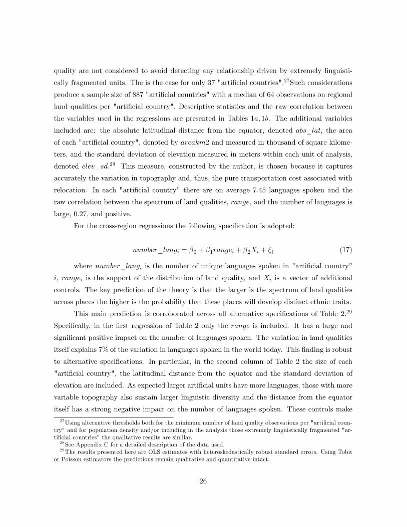
cally fragmented units. The is the case for only 37 "arti�cial countries".27Such considerations

produce a sample size of 887 "arti�cial countries" with a median of 64 observations on regional

land qualities per "arti�cial country". Descriptive statistics and the raw correlation between

the variables used in the regressions are presented in Tables 1a; 1b. The additional variables

included are: the absolute latitudinal distance from the equator, denoted abs_lat, the area

of each "arti�cial country", denoted by areakm2 and measured in thousand of square kilome-

ters, and the standard deviation of elevation measured in meters within each unit of analysis,

denoted elev_sd.28 This measure, constructed by the author, is chosen because it captures

accurately the variation in topography and, thus, the pure transportation cost associated with

relocation. In each "arti�cial country" there are on average 7:45 languages spoken and the

raw correlation between the spectrum of land qualities, range; and the number of languages is

large, 0:27; and positive.

For the cross-region regressions the following speci�cation is adopted:

number_langi = �0 + �1rangei + �2Xi + �i (17)

where number_langi is the number of unique languages spoken in "arti�cial country"

i, rangei is the support of the distribution of land quality, and Xi is a vector of additional

controls. The key prediction of the theory is that the larger is the spectrum of land qualities

across places the higher is the probability that these places will develop distinct ethnic traits.

This main prediction is corroborated across all alternative speci�cations of Table 2.29

Speci�cally, in the �rst regression of Table 2 only the range is included. It has a large and

signi�cant positive impact on the number of languages spoken. The variation in land qualities

itself explains 7% of the variation in languages spoken in the world today. This �nding is robust

to alternative speci�cations. In particular, in the second column of Table 2 the size of each

"arti�cial country", the latitudinal distance from the equator and the standard deviation of

elevation are included. As expected larger arti�cial units have more languages, those with more

variable topography also sustain larger linguistic diversity and the distance from the equator

itself has a strong negative impact on the number of languages spoken. These controls make

27Using alternative thresholds both for the minimum number of land quality observations per "arti�cial coun-try" and for population density and/or including in the analysis those extremely linguistically fragmented "ar-ti�cial countries" the qualitative results are similar.28See Appendix C for a detailed description of the data used.29The results presented here are OLS estimates with heteroskedastically robust standard errors. Using Tobit

or Poisson estimators the predictions remain qualitative and quantitative intact.

26

the coe¢ cient of range drop su¢ ciently, it remains however both economically and statistically

highly signi�cant. To the extent that the distance from the equator is associated with the

presence of seasonality and more unpredictable climate in general, the strong negative impact

of abs_lat on linguistic diversity is consistent with the prediction of the theory that areas

characterized by variation in productivity shocks will give rise to more homogeneous ethnic

entities. The introduction of the average quality of land, avg; and its interaction with the

range, avg_range, is designed to capture a potential diminishing e¤ect of the variation in land

quality on the formation of ethnic diversity as average land quality increases. Such e¤ect is

not detected, the e¤ect of the interaction is negative as expected but insigni�cant throughout.

Consequently, the interaction is dropped from the rest of the cross-region analysis.

In columns 3 and 4 of Table 2 I take advantage of the cross-region framework to explicitly

control for any idiosyncrasies of countries and continents. This is done by generating country

and continental dummies for those "arti�cial units" that fall into a single country and/or

a single continent respectively. Such inclusion of powerful controls, not possible in a cross-

country framework, allows to fully take into account any idiosyncratic country histories and

thus produce reliable estimates of the e¤ect of variation in land qualities on ethnic diversity.

The inclusion of country and continental �xed e¤ects does not a¤ect signi�cantly the estimated

coe¢ cient on range: One standard deviation increase in the spectrum of land qualities increases

by 1:56 the number of languages spoken contributing signi�cantly to the formation of ethnically

diverse societies. Both the latitudinal gradient, the standard deviation in elevation and the area

of each "arti�cial unit" enter signi�cantly and with the expected sign.

In the last two columns of table 2 speci�cation (17) including continental and country

�xed e¤ects is estimated separately for "arti�cial units" that are outside the tropics30 in column

(5) and those that fall within the tropics in column (6). These regressions allow to investigate

whether the identi�ed impact of the variation in land quality is driven by the climatic di¤erences

between the tropics and the rest of the geographic zones. Reassuringly, in both regressions the

e¤ect of range on linguistic diversity is precisely estimated at 5% level. However, the impact

of the variation in land quality is much larger in the tropics.

This section establishes that the variation in land quality across regions coupled with

the distance from the equator are signi�cant predictors of contemporary linguistic diversity.

The fact that these results obtain at an arbitrary level of aggregation and after controlling for

country and continental �xed e¤ects, highlights the importance of the forces identi�ed by the

30The tropics extent from 23:5 latitude degrees south to 23:5 latitude degrees north.

27

theory.

4.2.2 Cross-country analysis

Having established that the variation of land quality across regions a¤ects systematically the

number of languages spoken today i now proceed into investigating the relationship between

the spectrum of land qualities and ethnolinguistic fractionalization across countries.

Existing countries vary widely in the spectrum of land qualities that their territories

cover. In Appendix C maps with the regional land qualities for Lesotho and Malawi are

presented. A visual inspection of these maps reveals the homogeneity of land quality in Lesotho,

rangeLesotho = 0:37 compared to the apparent heterogeneity inherent to the land quality of

Malawi, rangeMalawi = 0:68. Note that these two countries have nonetheless comparable

overall levels of land quality, i.e. avgLesotho = 0:66 and avgMalawi = 0:56

Superimposing the languages spoken in Lesotho and Malawi, see maps in Appendix C, the

di¤erence is clear. The ethnically fragmented society of Malawi, ELFMalawi = 0:62; re�ects the

large underlying spectrum of land qualities compared to the ethnically homogeneous Lesotho,

ELFLesotho = 0:22.

As already mentioned the index of ethnolinguistic fractionalization, ELF , represents

the probability that two individuals randomly drawn from a country�s overall population will

belong to di¤erent ethnolinguistic groups. This implies that how people are distributed across

places a¤ects measured fractionalization. For example, should one region have the largest

fraction of the total population of the pair of places considered, this implies that even if these

two regions have di¤erent ethnicities the measured fractionalization will be low compared to

a case that these two places are equally densely populated.31 In this respect it is important

to consider that the theory provides a framework in which the probability that individuals

from two di¤erent regions will share common cultural traits, is endogenous to how similar the

productive structures of these regions are.

It is straightforward to manipulate (7) to elucidate how population density across places

a¤ects fractionalization. The expected fractionalization, E(ELF ); for a pair of places in par-

ticular reads:

E(ELF ) = (1� fT )

0@1� LiTLjT + L

iT

!2�

LjTLjT + L

jT

!21A (18)

31This is not a concern in the cross-region regressions given that the dependent variable is the count oflanguages spoken rather than a transformation of the count of people speaking these languages.

28

where (1 � fT ) is the probability that the two regions i and j will have di¤erent ethnic traits

and

1�

�LiT

LjT+LiT

�2��

LjTLjT+L

jT

�2!is the probability that two randomly chosen individuals

will belong to di¤erent regions. It is evident from (18) that the more unequally is population

distributed across places the lower would be fractionalization, ceteris paribus. In Appendix

A the regional population densities are expressed as a function of the regional land qualities

and it is shown that in the two-region case, conditional on the probability that two places will

have di¤erent ethnolinguistic elements, (1 � fT ); a more unequal distribution of land quality

decreases fractionalization.

Consequently, the gini coe¢ cient of land quality for each country, denoted by gini; is

constructed. As expected the gini of land quality is highly correlated (0:59) with how unequally

population density is distributed across regions within country in 1990.32, 33

Given the preceding discussion the following main speci�cation is adopted:

ELFi = a0 + a1rangei + a2avgi + a3avgirangei + a4ginii + �i (19)

where ELFi is the level of ethnolinguistic fractionalization in country i, avgi stands for

the average land quality in country i; rangei is the support of the distribution of land quality,

and ginii is the gini coe¢ cient measuring how unequally is land quality distributed across

regions in country i: The interaction term, avgirangei; is intended to capture a diminishing

e¤ect of variation in land quality as the average quality increases and �i is the error term.

Given the theory and the preceding remarks the predictions are:

a1 > 0; a2 = 0; a3 < 0; a4 < 0

In the regression analysis the sample is restricted in the following way. Only countries for

which there are at least 4 regions with information on land quality are included. Additionally,

to ensure that the �ndings are not driven by including in the regressions regions with very low,32To measure the latter a gini index of population density is constructed by the author for each country. The

population density data come from the Center for International Earth Science Information Network (CIESIN),Columbia University (2005) and were aggregated at the resolution level of the land quality data in order to makethe inequality indexes comparable. The data is available at http://sedac.ciesin.columbia.edu/gpw.33Results not shown also suggest that the gini coe¢ cient of land quality is strongly related (the correlation

is 0:55) to how clustered is land quality within a country, computed by the Moran�s I index, a commonlyused measure of spatial autocorrelation. That is, in countries with more unequal distribution of land qualitycontiguous regions are on average of similar land characteristics. Consequently, the adjacency of productivelysimilar regions would facilitate cross migration, due to low relocation costs, leading to lower fractionalization.Indeed, directly including in the regressions the level of clustering it enters negatively and decreases the coe¢ cientof gini, however, it is signi�cant only in regressions using as dependent variable the ethnic fractionalization indexderived by Alesina et. al. (2003).

29

or even zero, population density the relevant statistics are derived after taking out from each

country the 10% of the observations with the lowest population density.34 This amounts to

taking out places with a median population density of 0:12 individuals per square km. Such

considerations limit the sample size to on average 147 countries depending on the speci�cation.

Descriptive statistics and the raw correlation between the variables of interest are presented in

Tables 3a; 3b.

In Table 4 the regressors of the main speci�cation are added sequentially. The standard

errors presented all along are not corrected for heteroskedasticity since using White�s (1980)

general test the null hypothesis of homoskedasticity may not be rejected. Allowing for robust

standard errors the results are the same. In column 1 only the range is introduced and the

coe¢ cient is positive and statistically signi�cant. In column 2 the average land quality, avg, and

its interaction with the support of the distribution of land quality, avg_range; are added and

both the sign and the signi�cance of a1; a2; a3 are in accordance to the theoretical predictions.

The results of the main speci�cation (19) are presented in column 3 of Table 4. The

inclusion of gini as expected enters signi�cantly with the predicted negative sign improving

signi�cantly the regression �t and increases the coe¢ cient of range as would be expected given

the positive correlation between these two. These dimensions of the distribution of land quality

identi�ed explain 23% of the variation of contemporary ethnolinguistic fractionalization across

countries. As predicted, an increase in the spectrum of land qualities within country increases

ethnolinguistic fractionalization signi�cantly. The negative coe¢ cient of the interaction term

also implies that the e¤ect of variation in land quality diminishes as average land quality

improves. This is consistent with the view that as regions within country become increasingly

suitable for agricultural production it becomes easier to transfer region speci�c technology.

This lowers the barriers to mobility between populations residing in di¤erent areas leading to

lower fractionalization outcomes.

The impact of land heterogeneity, measured by the range, is also economically signi�cant.

A two standard deviation increase in the spectrum of land quality, evaluated at the mean of

land quality, increases fractionalization by 0:23: To better understand this magnitude note

34Using alternative thresholds both for the minimum number of observations per country and the regionalpopulation density the qualitative results are similar. Furthermore, we have also performed the regressionanalysis by weighting each region with the relevant population density as of 1990 and the results are largelyunchanged. A concern with this approach has to do with the fact that it does not re�ect the period duringwhich the fractionalization measures were collected, around 1950. For the same reason using directly the ginicoe¢ cient of regional population density as of 1990 in the main regression, although it delivers similar results,is not pursued further.

30

that the average di¤erence in ethnolinguistic fractionalization between a Sub-Saharan and a

non Sub-Saharan country is 0:33: All coe¢ cients for the range; gini and avg_range are fairly

precisely estimated and are signi�cant at 1% level. The average land quality, avg, is not

statistically di¤erent from zero which is consistent with the prediction that the average land

quality may impact the formation of ethnicities only through its interaction with the qualitative

heterogeneity across regions.

To make sure that the results are not subject to omitted variables bias, reverse causality

is less of a concern given the nature of the land quality characteristics,35 in Table 5 di¤erent

speci�cations are employed. I explore alternative hypotheses for the emergence of ethnicities,

namely, other geographical characteristics and historical contingencies.

Continental Fixed e¤ects

In the �rst column in Table 5 the main speci�cation is repeated. In the second col-

umn continental dummies for Sub-Saharan Africa (reg_ssa), Latin America and Caribbean

(reg_lac) and Western Europe (reg_we) are introduced, in order to make sure that the results

are not driven by a particular continent. The coe¢ cients of interest generally decrease remain,

though, both economically and statistically signi�cant. Note that the marginal overall e¤ect

of range does not change since both the direct and the interaction e¤ect decrease by roughly

the same magnitude. In fact the e¤ect of land quality heterogeneity, range, is signi�cantly

positive for all countries with avg � 0:69: For countries larger than this threshold (21 out of

147) the e¤ect of range is insigni�cant. Repeating the analysis after excluding all the countries

of Sub-Saharan Africa produces qualitatively similar results.

Other Geographical Characteristics

In the third column of table 5 geographic controls that could potentially a¤ect fraction-

alization are accounted for. As found in the cross-region regressions the distance from the

equator, denoted by abs_latitude, has a strong negative e¤ect on ethnolinguistic fractional-

ization. To the extent that distance from the equator increases seasonality, this is consistent

35The derivation of the land quality is partially based on the quality of the soil. This makes land qualitypossibly endogenous to the rise/duration of agriculture/herding. Controlling for the timing of the rise of agri-culture is not signi�cantly related to ethnic diversity and does not change the coe¢ cients of the variables ofinterest (results available upon request). A priori there is no reason to expect that ethnic diversity per se wouldsystematically impact the soil quality. Nevertheless, if for some reason ethnic diversity was reducing overall soilquality then the current results underestimate the true e¤ect of variation in land quality on ethnic diversity.

31

with the theory�s prediction that places subject to more variable productivity shocks should

display lower levels of fractionalization, ceteris paribus. This is a robust �nding, in column 5 of

Table 3 even after controlling for a host of continental, historical and geographic characteristics,

the coe¢ cient on abs_latitude remains signi�cant.36 The pure size of a country, denoted by

areakm2, perhaps surprisingly enters negatively although insigni�cant. The mean distance to

the nearest coastline or sea-navigable river, denoted by distcr, increases fractionalization and

this is conforming with the view that places which are increasingly isolated from water passages

have been experiencing limited population mixing, given any regional �uctuation in produc-

tivity, and thus should on average display higher ethnolinguistic fractionalization. It should

be noted noted, however, that mean distance from the sea, also captures the vulnerability of

places to both the incidence and the intensity of colonization. Thus, the coe¢ cient should be

cautiously interpreted.

An important geographic characteristic that might a¤ect the formation of languages and

ethnicities is the topography of each country. To account for elevation alternative measures are

used. The one presented here uses a new index constructed by the author, namely, the standard

deviation of elevation within a country, denoted elev_sd. This measure is chosen because it

captures accurately the variation in topography within a country. The results are similar using

average elevation, the % of mountainous land within country or the di¤erence between the

lowest and the highest point. The non-signi�cant e¤ect of the standard deviation of elevation

on fractionalization in column 3 of table 5, is driven by the fact that although Sub-Saharan

Africa, is the most fractionalized continent of the world, has an average standard deviation

of 0:28 km whereas for a non Sub-Saharan country the respective number averages 0:48 km.

Indeed, controlling for continental �xed e¤ects, see column 5; a more variable topography a¤ects

fractionalization positively and signi�cantly.

The inclusion of these additional geographical features reduces the magnitude of the

coe¢ cients of interest it does not alter, nevertheless, the qualitative predictions.

Historical Attributes

In column 4 of table 5 controls accounting for the variation in historical contingencies

across countries, are added. The log of the population density in 1500; lpd1500;37 enters

36Countries also vary in their latitudinal extent. Nevertheless, in all regressions explictly controlling for itcame highly insigni�cant and did not a¤ect the other estimates. Consequently, it was left out of the analysis.37This measure is highly correlated, around 0:56, with the experience of each region with statehood as con-

32

negatively but not signi�cantly and the year when each country gained independence, yrentry;

has a signi�cant impact of fractionalization. Speci�cally, the later is the year of independence

the higher is the level of fractionalization. This is consistent with the historical evidence which

suggests that modern states since their inception systematically attempted to homogenize the

population along ethnolinguistic dimensions. The expansion of public schooling, for example,

had exactly such an impact on linguistic diversity.38

Column 5 adds to the main speci�cation all the additional controls regarding geographic

characteristics, continental dummies and historical traits. The variables of interest remain both

economically and statistically signi�cant. These robustness checks underline the fundamental

role of the distribution of land quality in shaping ethnolinguistic diversity. At the same time

lpd1500 enters negatively and signi�cantly. This �nding is evidence that indeed contemporary

ethnic diversity is endogenous to the developmental history of each country as captured by the

population density in 1500.

So far, the empirical analysis includes countries whose ethnic mix is a relatively recent

phenomenon. United States, Brazil, Australia, Canada etc. fall into this category. However,

according to the theory the formation of ethnicities is an outcome of a long run process and

a stage of development when land was the dominant factor of production. In column 6 of

Table 5 the sample is restricted into countries whose percentage of indigenous population as of

1500 still comprises at least 75% of the current population mix. Under this speci�cation, the

results are even stronger and the distribution of land quality accounts for 27% of the observed

ethnolinguistic variation as opposed to 23% in column 1 which included all countries.

4.3 The E¤ect of Colonialism on Fractionalization

The component of ethnic diversity driven by the distribution of land quality, captured in the

main speci�cation (19), is the natural level of fractionalization, nat_ELF , that a region would

exhibit if left largely undisturbed. On the contrary, arti�cial fractionalization, denoted by

art_ELF , is the part of the observed fractionalization that is not driven by the characteristics

of land quality. According to the theory, in a world with common historical paths the natural

component would in principle explain an equal share of the fractionalization outcomes across

subsets of countries. However, it is certainly true that countries have experienced distinct

structed by Bockstette et al. (2002). Including both at the same time makes them insigni�cant. Consequently,i only include in the regressions the log of the population density in 1500.38Of course, the causality may run both directions since more fractionalized regions may lead to a later

emergence of modern states either because of being colonized or because of having a slower statehood formation.

33

historical events.

The previous section showed that the impact of heterogeneous land qualities on fraction-

alization is robust to alternative controls which accommodate for divergent historical paths,

with the latter however having also an independent e¤ect on contemporary ethnic diversity.

This section investigates in detail an issue that has received particular attention within eco-

nomics and this is the European colonization after the 15th century. Ample historical evidence

suggests that colonizers impacted the indigenous populations. The way they a¤ected the locals

varied widely from almost entirely eliminating the indigenous populations as in United States,

Australia, Argentina, Brazil to settling at very low levels in other places, as in Congo for ex-

ample. In several instances, they actively in�uenced preexisting groups by giving territories

to those that were not the initial claimants, ignoring the fact that another group was already

in the same territory or favoring some groups politically over others. Generally, the European

colonization created an imbalance in the mix of the indigenous populations, directly a¤ecting

the preexisting ethnic spectrum.

The discussion above implies that countries colonized by Europeans should exhibit frac-

tionalization outcomes endogenous to their colonial experience, the identity of the colonizers

and how intensely the colonizers settled,39 among other things. Table 6 presents the main spec-

i�cation (19) separately for countries that were colonized by European powers after the 15th

century and for those that were not. As expected the R2 coe¢ cient is larger for the sample of

countries that did not experience colonization. Speci�cally, the distribution of land quality ex-

plain 28% of the variation in the ethnolinguistic fractionalization for the non-colonized sample

and 19% for the colonized one.40 This �nding is consistent with the view that colonizers exten-

sively manipulated the underlying ethnicities augmenting signi�cantly the arti�cial component

of observed fractionalization outcomes. However, it is not only the man-made component

through which colonizers a¤ected the ethnolinguistic mix of the colonized world.

Historical accounts suggest that colonizers except for actively in�uencing the ethnic en-

dowment of each region also drew borders in an arbitrary way, see Herbst (2002) and Englebert

et al. (2002), essentially shaping the geographical spectrum whose ethnicities would compose

each country�s ethnic mix. The e¤ect of border drawing may be uncovered by looking at the

natural level of fractionalization, nat_ELF . This is derived using the predicted values of the

39The latter has been argued to depend on the very health environment of the colonized countries, Acemoglouet al. (2001).40Excluding the western European countries from the non-colonized sample the results become even stronger.

In particular, the distribution of land quality now explain 39% of the variation in the ethnolinguistic diversityin the non-colonized world.

34

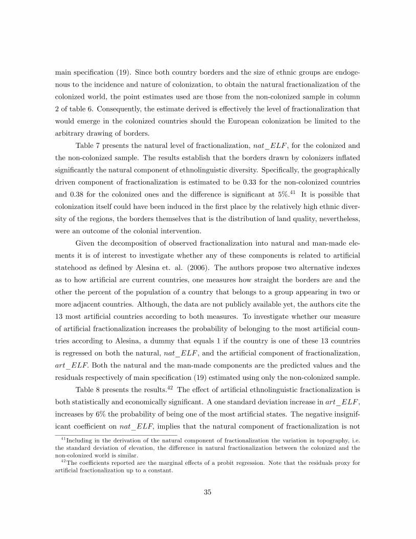
main speci�cation (19). Since both country borders and the size of ethnic groups are endoge-

nous to the incidence and nature of colonization, to obtain the natural fractionalization of the

colonized world, the point estimates used are those from the non-colonized sample in column

2 of table 6. Consequently, the estimate derived is e¤ectively the level of fractionalization that

would emerge in the colonized countries should the European colonization be limited to the

arbitrary drawing of borders.

Table 7 presents the natural level of fractionalization, nat_ELF , for the colonized and

the non-colonized sample. The results establish that the borders drawn by colonizers in�ated

signi�cantly the natural component of ethnolinguistic diversity. Speci�cally, the geographically

driven component of fractionalization is estimated to be 0:33 for the non-colonized countries

and 0:38 for the colonized ones and the di¤erence is signi�cant at 5%.41 It is possible that

colonization itself could have been induced in the �rst place by the relatively high ethnic diver-

sity of the regions, the borders themselves that is the distribution of land quality, nevertheless,

were an outcome of the colonial intervention.

Given the decomposition of observed fractionalization into natural and man-made ele-

ments it is of interest to investigate whether any of these components is related to arti�cial

statehood as de�ned by Alesina et. al. (2006). The authors propose two alternative indexes

as to how arti�cial are current countries, one measures how straight the borders are and the

other the percent of the population of a country that belongs to a group appearing in two or

more adjacent countries. Although, the data are not publicly available yet, the authors cite the

13 most arti�cial countries according to both measures. To investigate whether our measure

of arti�cial fractionalization increases the probability of belonging to the most arti�cial coun-

tries according to Alesina, a dummy that equals 1 if the country is one of these 13 countries

is regressed on both the natural, nat_ELF , and the arti�cial component of fractionalization,

art_ELF: Both the natural and the man-made components are the predicted values and the

residuals respectively of main speci�cation (19) estimated using only the non-colonized sample.

Table 8 presents the results.42 The e¤ect of arti�cial ethnolinguistic fractionalization is

both statistically and economically signi�cant. A one standard deviation increase in art_ELF ,

increases by 6% the probability of being one of the most arti�cial states. The negative insignif-

icant coe¢ cient on nat_ELF; implies that the natural component of fractionalization is not

41 Including in the derivation of the natural component of fractionalization the variation in topography, i.e.the standard deviation of elevation, the di¤erence in natural fractionalization between the colonized and thenon-colonized world is similar.42The coe¢ cients reported are the marginal e¤ects of a probit regression. Note that the residuals proxy for

arti�cial fractionalization up to a constant.

35

correlated with the measure of arti�cial statehood of Alesina et al. Naturally, until the entire

dataset for the state arti�ciality is released the results should be considered only as tentative.

Summarizing the impact of the European colonizers on the ethnolinguistic diversity the

evidence suggests that they substantially altered the ethnolinguistic endowment of the places

they colonized. Decomposing the existing fractionalization into a part driven by the distribution

of land quality and another one which is unrelated to the underlying land endowment, i.e.

man-made, the results suggest that colonizers increased both dimensions signi�cantly. Namely,

the European intervention imposed country borders that brought together regions whose land

characteristics could in principle sustain a wider ethnic spectrum. This was an outcome of the

intrinsic qualitative diversity of the land enclosed.

At the same time, their active manipulation of the original ethnolinguistic endowment,

including the introduction of their own ethnicities, substantially altered the man-made com-

ponent of the observed fractionalization tipping the balance in favor of an ethnic spectrum

whose identity and size was not a natural consequence of the primitive land characteristics.

These results suggest that contemporary fractionalization is endogenous to both the colonial

experience and the historical levels of development captured by the population density in 1500:

To the extent that state history has been shown to a¤ect contemporary economic outcomes

independently, the documented relationship between ethnolinguistic diversity and economic

outcomes should be cautiously interpreted.

5 Concluding Remarks

This research provides and tests a theory on the emergence of cultural diversity. The study

argues that the heterogeneity in the regional productive characteristics shaped the intensity

of population mixing across places. The transferability of region speci�c human capital and

the incentive to relocate, generated by the occurrence of regional productivity shocks, form the

basis of the theory.

Regions similar along their productive characteristics would display persistent population

mixing resulting in the formation of a common ethnolinguistic behavior. On the contrary,

among places characterized by dissimilar productive endowments, population mobility would

be limited leading to the formation of local ethnicities and languages giving rise to a wider

cultural spectrum.

The theory�s prediction about diversity in land quality and ethnic diversity has a striking

parallel to the literature on biodiversity and variation within species. Darwin�s observations

36

on �nches (1839) is of particular relevance. He observed that a certain ecological niche was

giving rise to a speci�c optimal shape of the �nches� beaks. So, ecologically diverse places

would bring about and sustain variation within �nches. Along the same lines this study argues

that a certain level of land quality generated speci�c human capital. Consequently, variation

in land qualities across regions contributed signi�cantly to the emergence and persistence of

ethnic diversity.

Using new detailed data on the distribution of land quality within and across countries

to proxy for the di¤erences in region speci�c human capital I �nd that a larger spectrum of

land qualities increases ethnic diversity. Both cross�region and a cross-country regressions

are examined. The cross-region framework is of particular signi�cance since the proposed

relationship between the variation in land quality and ethnic diversity obtains at an arbitrary

level of aggregation and after controlling for continental and country �xed e¤ects.

These results are robust to alternative speci�cations. In particular, controlling for ad-

ditional geographic characteristics and accounting for the divergent historical paths across

countries, the main predictions of the theory remain largely unchanged.

The empirical results also uncover the impact of state history on contemporary ethnic

diversity. In particular, exploring the role of European colonizers in shaping ethnolinguistic

diversity within the colonized world, interesting regularities are revealed. The arbitrary border

drawing becomes evident by looking at the level of natural fractionalization. This is system-

atically higher in the colonized world. The interfering of the colonizers, however, with the

local ethnicities was also widespread. The augmented man-made component of ethnic diversity

across the colonized countries attests to it. Preliminary results suggest that state arti�ciality as

measured by Alesina et. al. (2006) correlates strongly with the derived measure of man-made

fractionalization.

This research sheds new light on the emergence and the distribution of languages and

ethnicities within countries and constitutes a �rst step towards conceptualizing the natural and

man-made components of ethnic diversity.

The �ndings provide a stepping stone for further research. Equipped with a more sub-

stantive understanding of the economic origins and elements of cultural diversity, long standing

questions within development and growth literature may be readdressed. Issues like the for-

mation of states, the di¤usion of development, the inequality across ethnic groups, and the

causal e¤ect of ethnolinguistic diversity on economic outcomes in general, analyzed through

the proposed framework may o¤er new signi�cant insights.

37

6 Appendix

Appendix A - Proofs

Using Lemma 2 is straightforward to establish the properties of the size of the migration

between places, captured by (10) and (11).

Lemma 4 Conditional on positive migration in period t; that is if either (8) or (9) obtain in

the beginning of period t; the size of the population that migrates is

1. increasing (decreasing) in the relative regional productivity shock, �t; in case of migration

from j to i (i to j)@M j!i

t

@�t> 0 &

@M i!jt

@�t< 0

2. decreasing in the size of the erosion, "

@M j!it

@";@M i!j

t

@"< 0

3. decreasing in the region speci�c technology of the place of origin, hit; hjt

@M j!it

@hjt;@M i!j

t

@hit< 0

Proof of Lemma 4.

LetM j!it > 0 then there two distinct cases regarding the realization of the last migration

movement in period s.

Case 1: M j!is > 0:

Substituting (13) into (11) and simplifying:

M j!it =

Ljt�1[1� (�s�t )1

1�� (hjthjs)

"1�� ]

mj

mi (�t)� 11�� (hjt )

"1�� + 1

(20)

Case 2: M i!js > 0:

Substituting (12) into (11) and simplifying:

M j!it =

Ljt�1[1� (�s�t )1

1�� (hishjt )

"1�� ]

mj

mi (�t)� 11�� (hjt )

"1�� + 1

(21)

38

Direct di¤erentiation of (20) and (21) with respect to the variables of interest, produces the

results. A similar derivation applies to the case of migration from i! j; M i!jt . �

Proof of Lemma 3.

The steps are similar to those performed in the proof of Lemma 4. First, substitute

in (15) the two possible realizations of the past population densities, either (12) or (13), and

di¤erentiate with respect to the variables of interest. Repeat the same process for (16). This

completes the proof. �

The following Lemma summarizes the cases of migration occurrences.

Lemma 5 In any period t there are the following cases as to the occurrence or not of migration.

1. If last migration occurred in period s, 0 � s < t� 1; from region i to region j then

M i!jt > 0 iff �t < �s

�hishit

�"M j!it > 0 iff �t > �s

�hjth

is

�"M i!jt =M j!i

t = 0 iff �s

�hishit

�"� �t � �s

�hjth

is

�"

2. If last migration occurred in period s, 0 � s < t� 1; from region j to region i then

M i!jt > 0 iff �t < �s

�hjshit

��"M j!it > 0 iff �t > �s

�hjthjs

�"M i!jt =M j!i

t = 0 iff �s

�hjshit

��"� �t � �s

�hjthjs

�"Proof. Substituting the relevant ratio of the past population densities, either (12) or (13)

depending on the direction of the last migration, in both (10) and (11) and solving for the

required inequalities completes the proof. �

Proof of Proposition 1.

Under Assumption (A1) the ratio �t=�s may take three unique values either �min=�max or

�max=�min or 1. Obviously, �min=�max < 1 < �max=�min: In this case there will be no successive

migrations towards the same region. For example, for migration to occur in period t from j to

i it is necessary (though not su¢ cient, see Lemma 5) that �t > �s: This implies that �t = �max

39

and �s = �min: Consequently, it follows that since in period s migration also occurred, the

direction of this last migration could have only taken if place from region i towards region j;

i.e. �s = �min and �s�b = �max. Similar reasoning rules out successive migration towards region

i: This simpli�es the analysis considerably since one may focus only on the cases of Lemma 5

where a current migration, should it take place, is always in the opposite direction of the last

one. If �t=�s = �min=�max <�hjshit

��"migration occurs towards region j: So, conditional on

�min=�max; any regional pair characterized by higher " and higher region speci�c technology, hit;

will experience fewer (and also smaller in magnitude, see Lemma 4) migrations towards region

j. Similarly, migration occurs towards region i in period t i¤ �t=�s = �max=�min >�hjshit

�":

It is evident that the left hand-side increases as erosion increases, precipitating the end of

migratory movements towards region i:

Conditional on (A1) the probability that productivity shocks di¤er intertemporally, that

is �t=�s = �max=�min or �t=�s = �min=�max equals 2p(1�p): This is maximized at p = 1=2: It isalso obvious from 5 that the larger is �max=�min (equivalent the smaller is �min=�max) the more

probable will be migration. Consequently, increases in the variance of relative productivity

shocks var(�t) = p(1 � p)(�max � �min)2 increases the probability that the two regions will

share common cultural traits.

These observations taken together provide a sketch of the proof �

Interpreting Expected Fractionalization, (18), in terms of regional land qual-

ities:

Manipulating (18) may be rewritten as:

E(ELF ) = (1� fT ) LiT2LjT

+LjT2LiT

+ 1

!�1Noting (14) for example,43 the ratio of regional population densities is substituted ac-

cordingly and E(ELF ) may be rewritten as:

E(ELF ) = (1� fT )�mi

2mj+

mj

2mi+ 1

��1(22)

It is easy to show that conditional on the probability that two places will not share the

same cultural traits, (1� fT ); a more unequal distribution of the quality of land will decrease

measured fractionalization. For example, let mi > mj then an increase in mi and/or a decrease

43Using either (12) or (13) the analysis remains qualitatively similar, however E(elf) will be a more complicatedfunction of regional land qualities.

40

in mj will decrease E(ELF ). This obtains by di¤erentiating (22) with respect to mi and mj

accordingly.

This derivation highlights the fact that conditional on the probability that individuals

from two regions will have di¤erent ethnicities, an increase in the inequality of population den-

sity between these places, which is function of how unequally land quality itself is distributed,

as (22) shows, a¤ects negatively fractionalization outcomes.

41

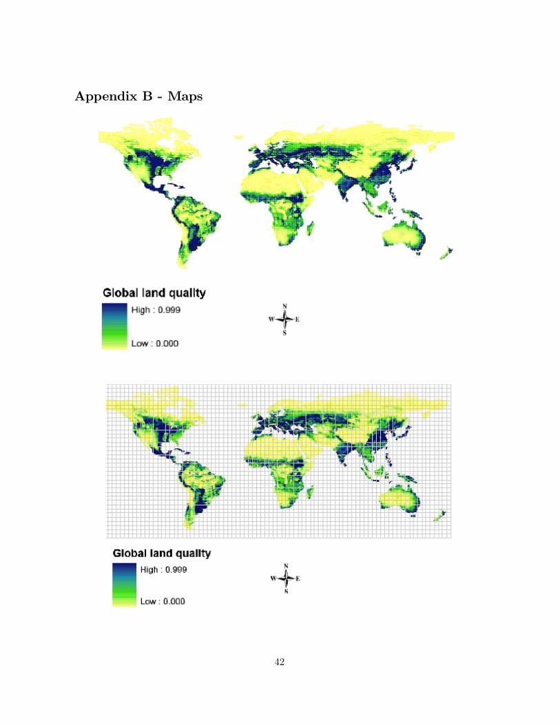
Appendix B - Maps

42

Table 1a: Summary Statistics for the Cross-Region Analysis

statistics number_lang range avg avg_range abs_lat elev_sd* areakm2mean 7.45 0.45 0.27 0.18 35.24 254.32 107.86

sd 8.89 0.33 0.27 0.19 19.11 257.70 35.13max 59.00 1.00 0.98 0.88 74.88 1733.14 151.24

min 1.00 0.00 0.00 0.00 0.38 0.83 6.71*in meters

number_lang : number of unique languages spoken within each "artificial country"; range : spectrum of landqualities within an "artificial country"; i.e. the difference in land quality between the region with the highestland quality from that with the lowest; avg : is the average land quality within "artificial country"; avg_range: theinteraction between range and avg; elev_sd: standard deviation of elevation within "artificial country"; abs_lat:"artificial country's" latitudinal distance from the equator; areakm2: size of each "artificial country" in sq. km.Data Sources: See Appendix D

Table 1b: The Correlation Matrix for the Cross-Region Analysis

number_lang range avg avg_range abs_lat elev_sd areakm2number_lang 1

range 0.27 1

avg 0.12 0.63 1avg_range 0.15 0.8 0.89 1

abs_lat -0.48 -0.3 -0.18 -0.16 1

elev_sd 0.14 0.17 0.01 0.07 -0.13 1

areakm2 0.43 0.29 0.06 0.13 -0.65 0.12 1number_lang : number of unique languages spoken within each "artificial country"; range : spectrum of landqualities within an "artificial country"; i.e. the difference in land quality between the region with the highestland quality from that with the lowest; avg : is the average land quality within "artificial country"; avg_range: theinteraction between range and avg; elev_sd: standard deviation of elevation within "artificial country"; abs_lat:"artificial country's" latitudinal distance from the equator; areakm2: size of each "artificial country" in sq. km.Data Sources: See Appendix D

Table 2: Main Specification and Robustness Checks in Cross-Region Regressions

Dependent Variable: Number of Languages Spoken

OLS OLS OLS OLS OLS OLS

Baseline

Elevation and Distance from the Equator

Continental fixed effects

Continental and Country fixed effects Non-Tropics Tropics

(1) (2) (3) (4) (5) (6)

range 7.188 4.067 4.109 4.743 1.663 6.892(9.28)*** (3.04)*** (4.32)*** (4.22)*** (2.37)** (2.10)**

avg 0.318 -1.011 -0.881 0.12 5.88(0.17) (0.84) (0.65) (0.15) (1.39)

avg_range -2.755(0.76)

areakm2 0.046 0.04 0.032 0.01 0.103(6.26)*** (5.48)*** (3.35)*** (1.88)* (5.83)***

abs_lat -0.146 -0.122 -0.216 -0.039 -0.559(8.84)*** (6.75)*** (7.41)*** (1.75)* (4.94)***

elev_sd 0.002 0.002 0.003 0.006 -0.002(1.67)* (1.80)* (2.23)** (3.94)*** (0.84)

R-squared 0.07 0.27 0.31 0.45 0.36 0.49

Observations 887 887 887 887 601 269OLS regressions with absolute value of robust t statistics in parentheses.* significant at 10%; ** significant at 5%; *** significant at 1%Regressions (4), (5) and (6) include both country and continental fixed effects.range: spectrum of land qualities within an "artificial country"; i.e. the difference in land quality between the region with the highest land quality from that with the lowest; avg: is the average land quality within "artificialcountry"; avg_range : the interaction between range and avg; elev_sd : standard deviation of elevation within"artificial country"; abs_lat : "artificial country's" latitudinal distance from the equator; areakm2 : size of each"artificial country" in square kilometers;Data Sources: See Appendix D

Appendix C - Maps

Upper map land quality; lower maplanguages and land quality

Upper map land quality; lower maplanguages and land quality45

Table 3a: Summary statistics for Cross-Country Analysis

statistics ELF range avg avg_range gini lpd1500 elev_sd* yrentry

mean 0.410 0.697 0.395 0.282 0.364 0.906 0.409 1927.120

sd 0.281 0.265 0.249 0.182 0.225 1.504 0.348 56.920

max 0.925 0.990 0.958 0.787 0.859 3.842 1.867 1993.000

min 0.001 0.002 0.003 0.000 0.028 -3.817 0.019 1816.000*in kilometers

ELF : ethnolinguistic fractionalization; range : spectrum of land qualities within the unit of analysis, country,

i.e. the difference in land quality between the region with the highest land quality from that with the lowest;

avg : is the average land quality within the unit of analysis, country; avg_range : the interaction between range

and avg; gini : the gini of coefficient of land quality within country; lpd1500 : log of the population density in 1500;

elev_sd : standard deviation of elevation within the unit of analysis, country; yrentry : year when modern state

obtained independence.Data Sources: See Appendix D

Table 3b: Correlation Matrix for Cross-Country Analysis

ELF range avg avg_range gini lpd1500 elev_sd yrentry

ELF 1.00

range 0.20 1.00

avg -0.21 0.15 1.00

avg_range -0.12 0.59 0.78 1.00

gini 0.12 0.23 -0.78 -0.52 1.00

lpd1500 -0.17 0.15 0.39 0.46 -0.34 1.00

elev_sd 0.10 0.33 -0.02 0.15 0.23 0.01 1.00

yrentry 0.36 -0.31 -0.20 -0.30 -0.06 -0.09 -0.21 1.00

ELF : ethnolinguistic fractionalization; range : spectrum of land qualities within the unit of analysis, country,

i.e. the difference in land quality between the region with the highest land quality from that with the lowest;

avg : is the average land quality within the unit of analysis, country; avg_range : the interaction between range

and avg; gini : the gini of coefficient of land quality within country; lpd1500 : log of the population density in 1500;

elev_sd : standard deviation of elevation within the unit of analysis, country; yrentry : year when modern state

obtained independence.

Data Sources: See Appendix D

Table 4: Main Specification for Cross-Country Analysis

Dependent Variable: ethnolinguistic fractionalization (ELF)

(1) (2) (3)

range 0.203 0.455 0.889(2.43)** (3.55)*** (5.73)***

avg 0.076 -0.283(0.42) (1.49)

avg_range -0.659 -1.21(2.18)** (3.90)***

gini -0.874(4.45)***

R-squared 0.04 0.13 0.23

Observatio 147 147 147

OLS regression with absolute value of t statistics in parentheses* significant at 10%; ** significant at 5%; *** significant at 1%

range : spectrum of land qualities within the unit of analysis, country, i.e.the difference in land quality between the region with the highest land quality fromthat with the lowest, avg: is the average land quality within country, avg_range:the interaction between range and avg, gini: the gini of coefficient of land qualitywithin country.

Data Sources: See Appendix D

Table 5: Main Specification and Robustness Checks

Dependent Variable: ethnolinguistic fractionalization (ELF)

BaselineContinental fixed effects

Additional geography

Historical controls

Full specification

Indigenous >75%

(1) (2) (3) (4) (5) (6)

range 0.925 0.641 0.692 0.889 0.668 1.032(5.92)*** (4.62)*** (4.71)*** (5.92)*** (4.87)*** (5.65)***

avg -0.198 -0.101 -0.261 -0.07 0.092 -0.241(0.79) (0.58) (1.54) (0.37) (0.52) (0.85)

avg_range -1.359 -0.653 -0.834 -1.043 -0.765 -1.422(3.85)*** (2.28)** (2.83)*** (3.39)*** (2.75)*** (3.73)***

gini -0.91 -0.416 -0.742 -0.626 -0.508 -0.921(4.30)*** (2.30)** (3.91)*** (3.27)*** (2.81)*** (3.78)***

reg_ssa 0.255 0.149(5.73)*** (2.48)**

reg_lac -0.102 -0.18(1.79)* (2.18)**

reg_we -0.172 0.075(2.70)*** -0.87

lpd1500 -0.02 -0.034(1.36) (2.03)**

yrentry 0.002 0.001(4.73)*** (1.86)*

abs_latitude -0.005 -0.004(4.27)*** (2.23)**

areakm2 -0.002 -0.001(1.61) (0.61)

distcr 0.202 0.105(4.14)*** (2.18)**

elev_sd 0.037 0.141(0.65) (2.37)**

R-squared 0.23 0.44 0.42 0.35 0.54 0.27

Observations 147 147 146 143 143 101OLS regressions with absolute value of t statistics in parentheses* significant at 10%; ** significant at 5%; *** significant at 1%range : spectrum of land qualities within country, i.e. the difference in land quality between the region withthe highest land quality from that with the lowest, avg: is the average land quality within country,avg_range : the interaction between range and avg, gini : the gini of coefficient of land quality within countryreg_ssa: dummy for Sub-Saharan countries, reg_lac : dummy for Latin-American and Caribbean countriesreg_we: dummy for Western European countries , abs_lat: country's latitudinal distance from the equatorareakm2 : size of each country in square kilometers; distcr : distance from centroid of country to nearestcoast or sea-navigable river (km); elev_sd : standard deviation of elevation within country; lpd1500:log of the population density in 1500 ; yrentry: year when modern state obtained independence.indigenous: percentage of indigenous population as of 1500 comprising more that 75% of the current populationData Sources: See Appendix D

Table 6: Colonization and Fractionalization

Dependent Variable: ethnolinguistic fractionalization (ELF)

Colonized by Europeans

Non-Colonized by Europeans

(1) (2)

range 0.792 0.914(3.80)*** (3.31)***

avg -0.324 -0.291(1.37) (0.79)

avg_range -0.892 -1.171(1.83)* (2.41)**

gini -0.813 -0.818(3.14)*** (2.63)**

R-squared 0.19 0.28

Observations 93 54OLS regressions with absolute value of t statistics in parentheses* significant at 10%; ** significant at 5%; *** significant at 1%range : spectrum of land qualities within the unit of analysis, country, i.e.the difference in land quality between the region with the highest land quality fromthat with the lowest; avg: is the average land quality within country; avg_range:the interaction between range and avg; gini: the gini of coefficient of land qualitywithin country; Data Sources: See Appendix D

Table 7: Colonization and Natural Fractionalization

nat_ELF if colonized: 0.38 nat_ELF if not colonized: 0.33

Pr(T < t) = 0.03nat_ELF : natural level of fractionalization computed using the predicted values of regression (2) in Table 6; Colonized : colonized by Europeans after 1500non-colonized : not colonized by Europeans after 1500

Table 8: Artificial Fractionalization and Artificial States

Dependent Variable: top 13 artificial states according to Alesina et al.

art_ELF 0.248(2.90)***

nat_ELF -0.04(0.03)

Observations 147Probit regression with absolute value of z statistics in parentheses* significant at 10%; ** significant at 5%; *** significant at 1%nat_ELF : natural level of fractionalization computed using the predicted values of regression (2) in Table 6; art_ELF: artificial level of fractionalization computedusing the residuals of regression (2) in Table 6;

Appendix D - Data Sources

Geographical Variables

elev_sd: standard deviation of elevation for actual countries and �arti�cial countries�.

Source: Constructed by the author using detailed grid level data on the average elevation

above sea level for each country. Available at the Atlas of Biosphere:

http://www.sage.wisc.edu:16080/atlas/

areakm2: land area (km2)

Source: Center for International Development, CID.44 For the cross-region analysis

the area is calculated by the author using the Haversine Formula, see http://www.movable-

type.co.uk/scripts/GIS-FAQ-5.1.html

distcr: distance from centroid of country to nearest coast or sea-navigable river (km)

Source: Center for International Development, CID.

abs_latitude: Absolute Latitudinal Distance from the Equator.

Source: The World Bank. Available from Development Research Institute, NYU. For

the cross-region analysis the distance from the equator is calculated by the author using the

centroid of each constructed regional unit.

Historical Variables

lpd1500: log population density in 1500.

Source: McEvedy and Jones (1978), "Atlas of World Population History,"

yrentry: year a country achieved independence.

Source: Fearon J., "Ethnic and Cultural Diversity by Country", originally from the

Correlated of War database (COW).

indigenous: percentage of indigenous population as of 1500 still comprising more that

75% of the current population mix.

Source: Putterman, L., 2007, World Migration Matrix, 1500 �2000, Brown University.

colonized: is a dummy equals 1 if a country was colonized by a European power after

1500 AD.

Source: "Determinants and Economic Consequences of Colonization: A Global Analysis"

Ertan, A., Putterman, L.,

Supplemented by entries from Encyclopedia Britannica where necessary.44All geographical data from CID are available at: http://www.ksg.harvard.edu/CID

50

References

[1] Acemoglu, D., Johnson, S., and Robinson, J., �The Colonial Origins of ComparativeDevelopment: An Empirical Investigation,�American Economic Review, December, XCI(2001a), 1369-1401.

[2] Alesina, A., Devleeschauwer, A., Easterly, W., Kurlat, S. and R. Wacziarg (2003) �Frac-tionalization�. Journal of Economic Growth, 8, 155-194.

[3] Alesina, A., Easterly, W., Matuszeski, M., (2006) �Arti�cial States�, Working Paper 12328.

[4] Alesina, A., and Spolaore, E., (1997) �On the Number and Size of Nations.�QuarterlyJournal of Economics. v112, 1027-1056.

[5] Ashraf, Q., and Michalopoulos S., (2006), �The Climatic Origins of the Neolithic Revolu-tion: A Theory of Long-Run Development via Climate-Induced Technological Progress�,SSRN: http://ssrn.com/abstract=903847

[6] Atlas Narodov Mira (Atlas of the People of the World). Moscow: Glavnoe UpravlenieGeodezii i Kartograi, 1964.Bruck, S.I., and V.S. Apenchenko (eds.).

[7] Barth, F., (1969). �Ethnic groups and boundaries: The social organization of culturaldi¤erence.�Boston: Little, Brown.

[8] Bellwood, P., �Early Agriculturalist Population Diasporas? Farming, Languages, andGenes�, Annual Review of Anthropology, Vol. 30. (2001), pp. 181-207.

[9] Bockstette, V., Chanda, A., Putterman, L.(2002) �States and Markets:the Advantage ofan Early Start�, Journal of Economic Growth Volume 7, Number 4, 347-369.

[10] Boyd, R., and P.J. Richardson., (1985), �Culture and the Evolutionary Process� (Univer-sity of Chicago Press, Chicago).

[11] Boserup, E., (1965). �The Conditions of Agricultural Progress�, (Aldine Publishing Com-pany, Chicago).

[12] Botticini, M., Eckstein, Z., (2005) �From Farmers to Merchants, Voluntary Conversionsand Diaspora: A Human Capital Interpretation of Jewish History�, Journal of EconomicHistory 65, no. 4, 922-48.

[13] Center for International Earth Science Information Network (CIESIN), Columbia Univer-sity; and Centro Internacional de Agricultura Tropical (CIAT). 2005. Gridded Populationof the World Version 3 (GPWv3) Palisades, NY: Socioeconomic Data and ApplicationsCenter (SEDAC), Columbia.

[14] Curtin, P., (1984) �Cross-Cultural Trade in World History�, Cambridge: Cambridge Uni-versity Press.

[15] Darwin, C. (1839) �The Voyage of the Beagle�, Available at: http://www.online-literature.com/darwin/voyage_beagle/

[16] Easterly, W., and Levine, R., (1997) �Africa�s growth tragedy: Policies and Ethnic divi-sions�, Quarterly Journal of Economics, 112(4):1203-50.

51

[17] Englebert, P., Tarango, S., and Carter, M., (2002) �Dismemberment and Su¤ocation: AContribution to the Debate on African Boundaries.�Comparative Political Studies. v35:10,1093-1118.

[18] Esteban, J., Ray., D., (2007) �On the salience of ethnic con�ict�, Working Paper.

[19] Fearon, J., (2003) �Ethnic Structure and Cultural Diversity by Country�, Journal of Eco-nomic Growth, 8(2). 195-222.

[20] Fearon, J., Laitin, D. (2002) �Ethnicity, Insurgency and Civil War�, American PoliticalScience Review.

[21] Galor, O. and Weil, D.N., (2000), �Population, Technology and Growth: From the Malthu-sian Regime to the Demographic Transition.�American Economic Review 110, 806-828.

[22] Geertz, C., (1967) �Old societies and new states: The quest for modernity in Asia andAfrica.�New York: Free Press.

[23] Gray, R. Atkinson, Q. (2003), �Language-tree divergence times support the Anatoliantheory of Indo-European origin�, Nature, 426, 435-439

[24] Hale, H., (2004) �Explaining Ethnicity�, Comparative Political Studies 2004; 37- 458.

[25] Herbst, J., (2002) �State and Power in Africa�. Princeton, NJ: Princeton University Press.

[26] La Porta, R., Lopez de Silanes, F., Shleifer, A., Vishny, R., (1999) �The Quality of Gov-ernment�Journal of Law Economics and Organization, 315-388.

[27] Michalopoulos, S., (2007b),�The Origins of Ethnolinguistic Diversity: Natural and Arti�-cial Components in the Process of Development�, Brown University.

[28] Montalvo, and Reynal-Querol, (2005), �Ethnic polarization, potential con�ict and civilwar, American Economic Review�, 2005.

[29] Nichols, J.,(1997) �Modeling Ancient Population Structures and Movement in Linguistics�.Annual Review of Anthropology, Vol. 26., 359-384.

[30] Nichols, J., (1997b). �Chechen phonology�, In Phonologies of Asia and Africa, ed. ASKaye, P Daniels, 941-71. Bloomington, Ind:Eisenbrauns.

[31] Ramankutty, N., J.A. Foley , J. Norman, and K. McSweeney, �The global distributionof cultivable lands:current patterns and sensitivity to possible climate change�, GlobalEcology & Biogeography (2002) 11, 377�392.

[32] Renfrew, C., (1992) �Archaeology, Genetics and Linguistic Diversity�, Man, New Series,Vol. 27, No. 3, 445-478.

[33] Renfrew, C., (2000) �At the edge of knowability: Towards a Prehistory of Languages�,Cambridge Archaelogical Journal, Vol. 10, No. 1, 7-34.

[34] Spolaore, E., and Wacziarg R., (2006), �The Di¤usion of Development,�NBER WorkingPaper #12153.

[35] Williamson J., (2006), �Poverty Traps Distance and Diversity: The Migration Connec-tion�, NBER Working Paper #12549.

52