The optimizing-simulator: An illustration using the military airlift problem

14

The Optimizing-Simulator: An IllustrationUsing the Military Airlift Problem

TONGQIANG TONY WU and WARREN B. POWELL

Princeton University

and

ALAN WHISMAN

Air Mobility Command Retired

There have been two primary modeling and algorithmic strategies for modeling operational prob-lems in transportation and logistics: simulation, offering tremendous modeling flexibility, and op-timization, which offers the intelligence of math programming. Each offers significant theoreticaland practical advantages. In this article, we show that you can model complex problems using arange of decision functions, including both rule-based and cost-based logic, and spanning differentclasses of information. We show how different types of decision functions can be designed using upto four classes of information. The choice of which information classes to use is a modeling choice,and requires making specific choices in the representation of the problem. We illustrate these ideasin the context of modeling military airlift, where simulation and optimization have been viewed ascompeting methodologies. Our goal is to show that these are simply different flavors of a series ofintegrated modeling strategies.

Categories and Subject Descriptors: I.6.1 [Simulation and Modeling]: Simulation theory; I.6.3[Simulation and Modeling]: Applications; I.6.5 [Simulation and Modeling]: Model Develop-ment—Modeling methodologies

General Terms: Algorithms

Additional Key Words and Phrases: Approximate dynamic programming, military logistics, controlof simulation, modeling information, optimizing-simulator

ACM Reference Format:Wu, T. T., Powell, W. B., and Whisman, A. 2009. The optimizing-simulator: An illustration usingthe military airlift problem. ACM Trans. Model. Comput. Simul., 19, 3, Article 14 (June 2009), 31pages. DOI = 10.1145/1540530.1540535 http://doi.acm.org/ 10.1145/1540530.1540535

This research was supported in part by grant AFOSR contract FA9550-08-1-0195.Authors’ addresses: T. T. Wu and W. B. Powell, Dept. of Operations Research and Financial En-gineering, Princeton University, Princeton, NJ 08544; email: [email protected]; A. Whisman,Air Mobility Command, Scott Air Force Base, IL 62225.Permission to make digital or hard copies of part or all of this work for personal or classroom useis granted without fee provided that copies are not made or distributed for profit or commercialadvantage and that copies show this notice on the first page or initial screen of a display alongwith the full citation. Copyrights for components of this work owned by others than ACM must behonored. Abstracting with credit is permitted. To copy otherwise, to republish, to post on servers,to redistribute to lists, or to use any component of this work in other works requires prior specificpermission and/or a fee. Permissions may be requested from Publications Dept., ACM, Inc., 2 PennPlaza, Suite 701, New York, NY 10121-0701 USA, fax +1 (212) 869-0481, or [email protected]© 2009 ACM 1049-3301/2009/06-ART14 $10.00DOI 10.1145/1540530.1540535 http://doi.acm.org/10.1145/1540530.1540535

ACM Transactions on Modeling and Computer Simulation, Vol. 19, No. 3, Article 14, Publication date: June 2009.

14:2 • T. T. Wu et al.

1. INTRODUCTION

Complex operational problems, such as those that arise in transportation andlogistics, have long been modeled using simulation or optimization. Typically,these are viewed as competing approaches, each offering benefits over the other.Simulation offers significant flexibility in the modeling of complex operationalconditions, and in particular is able to handle various forms of uncertainty. Op-timization offers intelligent decisions that often allow models to adapt quicklyto new datasets (simulation models often require recalibrating decision rules),and offer additional benefits such as dual variables. In the desire for good solu-tions, optimization seeks to find the best solution, but typically requires makinga number of simplifications.

We encountered the competition between simulation and optimization inthe context of modeling the military airlift problem faced by the analysis groupat the Airlift Mobility Command (AMC). The military airlift problem dealswith effectively routing a fleet of aircraft to deliver loads of people and goods(troops, equipment, food, and other forms of freight) from different origins todifferent destinations as quickly as possible under a variety of constraints.In the parlance of military operations, loads (or demands) are referred to asrequirements. Cargo aircraft come in a variety of sizes, and it is not unusualfor a single requirement to need multiple aircraft. If the requirement includespeople, the aircraft has to be configured with passenger seats. Other issuesinclude maintenance, airbase capacity, weather, and the challenge of routingaircraft through friendly airspaces.

There are two major classes of models that have been used to solve themilitary airlift (and closely related sealift) problem: cost-based optimizationmodels [Morton et al. 1996; Rosenthal et al. 1997; Baker et al. 2002], and rule-based simulation models, such as MASS (Mobility Analysis Support System)and AMOS (Air Mobility Operations Simulator), which are heavily used withinthe AMC. The analysis group at AMC has preferred AMOS because it offerstremendous flexibility, as well as the ability to handle uncertainty. However,simulation models require that the user specify a series of rules to obtain re-alistic behaviors. Optimization models, on the other hand, avoid the need tospecify various decision rules, but they force the analyst to manipulate the be-havior of the model (the decisions that are made) by changing the objectivefunction. While optimal solutions are viewed as the gold standard in modeling,it is a simple fact that for many applications, objective functions are little morethan coarse approximations of the goals of an operation.

Our strategy should not be confused with simulation-optimization, which iswell-known within the simulation community (see, for example, the excellentreviews Swisher et al. [2003] and Fu [2002]). This strategy typically assumesan often myopic parameterized policy, where the goal is to find the best settingsfor one or more parameters. For our class of applications, we are trying to con-struct a simulation model that can directly compete with a math programmingmodel, while retaining many of the important features that classical simula-tion methods bring to the table. For example, we need decisions that considertheir impact on the future. At the same time, we need a model that will handle


The Optimizing-Simulator: An Illustration Using the Military Airlift Problem • 14:3

uncertainty and a high level of detail, features that we take for granted insimulation models.

This article proposes to bring together the simulation and optimization com-munities who work on transportation and logistics. We do this by combiningmath programming, approximate dynamic programming, and simulation, witha strong dependence on machine learning. From the perspective of the simula-tion community, it will look as if we are running a simulation iteratively, duringwhich we can estimate the value of being in a state (dynamic programming), andwe can also measure the degree to which we are matching exogenously speci-fied patterns of behavior (a form of supervisory control from the reinforcement-learning community). At each point in time, we use math programming to solvesequences of deterministic optimization problems. Math programming allowsus to optimize at a point in time, while dynamic programming allows us tooptimize over time. The pattern matching allows us to bridge the gap betweencost-based optimization and rule-based simulation.

This strategy has the effect of allowing us to build a family of decision func-tions with up to four classes of information: (1) the physical state (what we knowabout the system now), (2) forecasts of exogenous information events (new cus-tomer demands, equipment failures, weather delays), (3) forecasts of the impactof decisions now on the future (giving rise to value functions used in dynamicprogramming), and (4) forecasts of decisions (which we represent as patterns).The last three classes of information are all a form of forecast. If we just usethe first class, we get a classical simulation using a myopic policy, althoughthese come in two flavors: rule-based (popular in simulation) and cost-based(popular in the transportation community when solving dynamic problems). Ifwe use the second information class, we obtain a rolling-horizon procedure. Thethird class of information uses approximate dynamic programming to estimatethe value of being in a state. The fourth class allows us to combine cost-basedlogic (required for any optimization model) with particular types of rules (forexample, “we prefer to use C-17s for loads originating in Europe”). This classintroduces the use of proximal point algorithms. We claim that any existingmodeling and algorithmic strategy can be classified in terms of its use of thesefour classes of information.

The central contribution of this article is to identify how simulation andoptimization can be combined to address complex modeling problems that arisein transportation and logistics, illustrated using the context of a military airliftapplication. This problem class has traditionally been solved using classicaldeterministic optimization methods or simulation, with each approach havingsignificant strengths and weaknesses. We show how cost-based and rule-basedlogic can be combined within this broad framework. We illustrate these ideasusing an actual airlift simulation to show that we can vary the informationcontent of decisions to produce decisions with increasing levels of sophistication.

We begin in Section 2 with a review of the field of modeling military mobilityproblems (this is how this community refers to this problem class). More thanjust a literature review, this section allows us to contrast the modeling styles ofdifferent communities, including deterministic math programming, simulation,


14:4 • T. T. Wu et al.

and stochastic programming. In Section 3 we provide our own model of the airliftproblem, providing only enough notation to illustrate the important modelingprinciples. Section 4 shows how we can create different decision functions bymodeling the information available to make a decision. We also discuss rule-based and cost-based functions, and show how these can be integrated intoa single, general decision function that uses all four classes of information. InSection 5 we simulate all the different information classes, and show that as weincrease the information (that is, use additional information classes) we obtainbetter solutions, measured in terms of throughput, a common measure used inthe military, and realism—reflected by our ability to match desired patterns ofbehavior. Section 6 concludes the article.

2. MODELING OF MILITARY MOBILITY PROBLEMS

This section provides a summary of different modeling strategies for mili-tary mobility problems: air and sea. After providing a review of the militarymobility literature in Section 2.1, we briefly summarize the three primarymodeling strategies that have been used in this area: deterministic linear pro-gramming (Section 2.2), simulation (Section 2.3), and stochastic programming(Section 2.4). The modeling of mobility problems is unusual in that it has beenapproached in detail by all three communities. We present these models in onlyenough detail to allow us to contrast the different modeling styles.

2.1 The History of Mobility Modeling

Ferguson and Dantzig [1955] is one of the first to apply mathematical modelsto air-based transportation. Subsequently, numerous studies were conductedon the application of optimization modeling to the military airlift problem.Several mathematical modeling formulations for military airlift operations aredescribed by Mattock et al. [1995]. The RAND Corporation published a veryextensive analysis of airfield capacity in Stucker and Berg [1999]. Accordingto Baker et al. [2002], research on air mobility optimization at the Naval Post-graduate School (NPS) started with the Mobility Optimization Model (MOM).This model is described in Wing et al. [1991] and concentrates on both sealiftand airlift operations. Therefore, the MOM model is not designed to capture thecharacteristics specific to airlift operations, but it is a good model in the sensethat it is time-dependent. THRUPUT, a general airlift model developed byYost [1994], captures the specifics of airlift operations but is static. The UnitedStates Air Force Studies and Analyses Agency in the Pentagon asked NPS tocombine the MOM and THRUPUT models into one model that would be timedependent and would also capture the specifics of airlift operations [Baker et al.2002]. The resulting model is called THRUPUT II, described in detail in Rosen-thal et al. [1997]. During the development of THRUPUT II at NPS, a groupat RAND developed a similar model called CONOP (CONcept of OPerations),described in Killingsworth and Melody [1997]. The THRUPUT II and CONOPmodels each possessed several features that the other lacked. Therefore, theNaval Postgraduate School and the RAND Corporation merged the two modelsinto NRMO (NPS/RAND Mobility Optimizer), described in Baker et al. [2002].



Crino et al. [2004] introduced the group-theoretic tabu search method to solvethe theater distribution vehicle routing and scheduling problem. Their heuristicmethodology evaluates and determines the routing and scheduling of multi-modal theater transportation assets at the individual asset operational level.

A number of simulation models have also been proposed for airlift problems(and related problems in military logistics). Schank et al. [1991] review severaldeterministic simulation models. Burke et al. [2004] at the Argonne NationalLaboratory developed a model called TRANSCAP (Transportation SystemCapability) to simulate the deployment of forces from Army bases. The heartof TRANSCAP is the discrete-event simulation module developed in MODSIMIII. Perhaps the most widely used model at the Air Mobility Command isAMOS which is a discrete-event worldwide airlift simulation model used instrategic and theater operations to deploy military and commercial airliftassets. It was once the standard for all airlift problems in AMC, and all airliftstudies were compared with the results produced by the AMOS model. AMOSprovides for a very high level of detail, allowing AMC to run analyses on awide variety of issues.

One feature of simulation models is their ability to handle uncertainty, andas a result there has been a steady level of academic attention toward incor-porating uncertainty into optimization models. Dantzig and Ferguson [1956]is one of the first to study uncertain customer demands in the airlift prob-lem. Midler and Wollmer [1969] also takes into account stochastic cargo re-quirements. This work formulates two two-stage stochastic linear programmingmodels: a monthly planning model, and a daily operational model for the flightscheduling. Goggins [1995] extended Throughput II [Rosenthal et al. 1997] toa two-stage stochastic linear program to address the uncertainty of aircraftreliability. Niemi [2000] expands the NRMO model to incorporate stochasticground times through a two-stage stochastic programming model. To reducethe number of scenarios for a tractable solution, the model assumes that theset of scenarios is identical for each airfield and time period and a scenario isdetermined by the outcomes of repair times of different types of aircraft. Theresulting stochastic programming model has an equivalent deterministic lin-ear programming formulation. Granger et al. [2001] compared the simulationmodel and the network approximation model for the impact of stochastic fly-ing times and ground times on a simplified airlift network (one origin aerialport of embarkation (APOE), three intermediate airfields and one destinationaerial port of debarkation (APOD)). Based on the study, they suspect that acombination of simulation and network optimization models should yield muchbetter performance than either one of these alone. Such an approach woulduse a network model to explore the variable space and identify parameter val-ues that promise improvements in system performance, then validate theseby simulation. Morton et al. [2002] developed the Stochastic Sealift Deploy-ment Model (SSDM), a multi-stage stochastic programming model to plan thewartime, sealift deployment of military cargo subject to stochastic attack. Theyused scenarios to represent the possibility of random attacks.

A related method in Yost and Washburn [2000] combines linear program-ming with partially observable Markov decision processes to a military attack


14:6 • T. T. Wu et al.

problem in which aircraft attack targets in a series of stages. They assume thatthe expected value of the reward (destroyed targets) and resource (weapon) con-sumption are known for each policy where a policy is chosen in a finite feasibleset. Their method requires that the number of possible states of each object besmall and the resource constraints be satisfied on the average. In the militaryairlift problem, the number of possible states is very large, as are the number ofactions and outcomes. As a result, we could not have the expected value of thereward before we solve the problem. In general, we require that the resourceconstraints are strictly satisfied in a military airlift problem.

2.2 The NRMO Model

The NRMO model has been in development since 1996 and has been employedin several airlift studies. For a detailed review of the NRMO model, includinga mathematical description, see Baker et al. [2002]. The goal of the NRMOmodel is to move equipment and personnel in a timely fashion from a set oforigin bases to a set of destination bases using a fixed fleet of aircraft withdiffering characteristics. This deployment is driven by the movement and de-livery requirements specified in a list called the Time-Phased Force DeploymentDocument (or Dataset) (TPFDD). This list essentially contains the cargo andtroops, along with their attributes, that must be delivered to each of the basesof a given military scenario.

Aircraft types for the NRMO runs reported by Baker et al. [2002] includeC-5, C-17, C-141, Boeing 747, KC-10, and KC-135. Different types of aircrafthave different features, such as passenger and cargo-carrying capacity, airfieldcapacity consumed, range-payload curve, and so on. The range-payload curvespecifies the weight that an aircraft can carry given a distance traveled. Theserange-payload curves are piecewise linear concave.

The activities in NRMO are represented using three time-space networks:the first one flows aircraft, the second the cargo (freight and passengers) andthe third flows crews. Cargo and troops are carried from the onload aerial portof embarkation (APOE) to either the offload aerial port of debarkation (APOD)or the forward operating base (FOB). Certain requirements need to be deliveredto the FOB via some other means of transportation after being offloaded at theAPOD. Some aircraft, however, can bypass the APOD and deliver directly tothe FOB. Each requirement starts at a specific APOE dictated by the TPFDDand then is either dropped off at an APOD or a FOB.

NRMO makes decisions about which aircraft to assign to which require-ment, which freight will move on an aircraft, which crew will handle a move,as well as variables that manage the allocation of aircraft between roles suchas long range, intertheater operations and shorter, shuttle missions within atheater. The model can even handle the assignment of KC-10s between the roleof strategic cargo hauler and midair refueler.

In the model, NRMO minimizes a rather complex objective function thatis based on several costs assigned to the decisions. There are a variety ofcosts, including hard operating costs (fuel, maintenance) and soft costs toencourage desirable behaviors. For example, NRMO assigns a cost to penalize



deliveries of cargo or troops that arrive after the required delivery date.This penalty structure charges a heavier penalty the later the requirementis delivered. Another term penalizes the cargo that is simply not delivered.The objective also penalizes reassignments of cargo and deadheading crews.Last, the objective function offers a small reward for planes that remain at anAPOE, as these bases are often in the continental US and are therefore closeto the home bases of most planes. The idea behind this reward is to accountfor uncertainty in the world of war and to keep unused planes well positionedin case of unforeseen contingencies.

The constraints of the model can be grouped into seven categories: (1) demandsatisfaction; (2) flow balance of aircraft, cargo and crews; (3) aircraft delivery ca-pacity for cargo and passengers; (4) the number of shuttle and tanker missionsper period; (5) initial allocation of aircraft and crews; (6) the usage of aircraft ofeach type; and (7) aircraft handling capacity at airfields. A general statementof the model (see Baker et al. [2002] for a detailed description) is given by:

min(xt ),t=0,... ,T

T∑t=0

ct xt (1)

subject to

At xt −t∑

τ=1

Bt−τ,t xt−τ = Rt , t = 0, 1, . . . , T, (2)

Dt xt ≤ ut , t = 0, 1, . . . , T, (3)xt ≥ 0, t = 0, 1, . . . , T, (4)

where,

t = the time at which an activity begins,τ = the time required to complete an action,

At = incidence matrix giving the elements of xt that representdepartures from time t,

Bt−τ,t = incidence matrix giving the elements of xt that representflows arriving at time t,

Dt = incidence matrix capturing flows that are jointly con-strained,

ut = upper bounds on flows,Rt = the resources available at time t,xt = the decision vector at time t, where an element might be xti j

telling us if aircraft i is assigned to requirement j at timet,

ct = the cost vector at time t.

NRMO is implemented with the algebraic modeling language GAMS [Brookeet al. 1992], which facilitates the handling of states. Each state is identified byan index combination of elements drawn from sets of aircraft attributes suchas time periods, requirements, cargo types, aircraft types, bases, and routes.


14:8 • T. T. Wu et al.

An example of an index combination would be an aircraft of a certain type de-livering a certain requirement on a certain route departing at a certain time.Only feasible index combinations are considered in the model so that the com-putation becomes tractable. The information in the NRMO model is capturedin the TPFDD, which is known at the beginning of the horizon.

NRMO requires that the behavior of the model be governed by a cost model(which simulators do not require). The use of a cost model minimizes the needfor extensive tables of rules to produce good behaviors. The optimization modelalso responds in a natural way to changes in the input data (for example, anincrease in the capacity of an airbase will not produce a decrease in overallthroughput). But linear programming formulations suffer from weaknesses. Asignificant limitation is the difficulty in modeling complex system dynamics.For example, a simulation model can include logic such as, “if there are fouraircraft occupying all the parking spaces, a fifth aircraft will have to be pulledoff the runway where it cannot be refueled or repaired.” In addition, linearprogramming models cannot directly model the evolution of information. Thislimits their use in analyzing strategies that directly affect uncertainty (Whatis the impact of last-minute requests on operational efficiency? What is the costof sending an aircraft through an airbase with limited maintenance facilities,where the aircraft might break down?).

2.3 The AMOS Model

AMOS is a rule-based simulation model. A rough approximation of the rulesproceeds as follows. AMOS starts with the first available aircraft, and thentries to see if the aircraft can move the first requirement that needs to be moved(there is logic to check if there is an aircraft at the origin of the requirement, butotherwise the distance the aircraft has to travel is ignored). Given an aircraftand requirement, the next problem is to evaluate the assignment. For simpletransportation models, this step is trivial (e.g. a cost per mile times the numberof miles). For more complex transportation problems (managing drivers), it isnecessary to go through a more complex set of calculations that depend on thehours of service. For the military airlift problem, moving an aircraft from, say,the East Coast to India, requires moving through a sequence of intermediateairbases that have to be checked for capacity availability. This step is fairlyexpensive, so it is difficult to evaluate all possible combinations of aircraft andrequirements. If AMOS determines that an assignment is infeasible, it simplymoves to the next aircraft in the list.

We note that it is traditional to describe simulation models such as this withvirtually no notation. We can provide a very high level notational system bydefining:

St = the state vector of the system at time t, giving what weknow about the system at time t, such as the current statusof aircraft and requirements;

X π (St) = the function that returns a decision, xt , given informationSt , when we are using policy π , where π is simply an indexidentifying the specific function being used;



Attack

Tim

e

t1

t2

t3

t4

Fig. 1. The single attack scenario tree used in SSDM.

xt = the vector of decisions at time t (just as in the NRMOmodel);

Wt = exogenous information arriving between t − 1 and t;SM (St , xt , Wt+1) = the transition function (sometimes called the system

model) that gives the state St+1, at time t + 1, given thatwe are in state St , make decision xt , and observe new ex-ogenous information Wt+1.

Given a policy (that is, a decision function X π (St)), a simulation model can beviewed as consisting of nothing more than the two equations:

xt ← X π (St), (5)St+1 ← SM (St , xt , Wt+1(ω)). (6)

A more complete model would specify the state variable and transition functionin greater detail. Note that we do not have an objective function.

2.4 The SSDM Model

The Stochastic Sealift Deployment Model (SSDM) [Morton et al. 2002] is a mul-tistage stochastic mixed-integer program designed to hedge against potentialenemy attacks on seaports of debarkation (SPODs) with probabilistic knowl-edge of the time, location and severity of the attacks. They test the model on anetwork with two SPODs (the number actually used in the Gulf War) and otherlocations such as a seaport of embarkation (SPOE) and locations near SPODswhere ships wait to enter berths. To keep the model computationally tractable,they assumed only a single biological attack can occur. Thus, associated witheach possible outcome (scenario in the language of stochastic programming) iswhether or not an attack occurs. We assume that there is a finite set of scenar-ios �, and we let ω ∈ � be a single scenario. If scenario ω occurs, t(ω) is thetime at which it occurs. They then let T (ω) = {0, . . . , t(ω) − 1} be the set of timeperiods preceding an attack that occurs at time t(ω). This structure results in ascenario tree that grows linearly with the number of time periods, as illustratedin Figure 1. The stochastic programming model for SSDM can then be written:

minxt (ω),t=0,... ,T,ω∈�

∑ω∈�

T∑t=0

p(ω)ct(ω)xt(ω), (7)


14:10 • T. T. Wu et al.

subject to

At xt(ω) −t∑

τ=1

�t−τ,t xt−τ (ω) = Rt(ω) t = 0, 1, . . . , T, ω ∈ �,

Bt xt(ω) ≤ ut(ω), t = 0, 1, . . . , T, ω ∈ �,xt(ω) = xt(ω′), for all t ∈ T (ω) ∩ T (ω′), ω ∈ �, (8)xt(ω) ≥ 0 and integer, for all t = 0, 1, . . . , T, ω ∈ �.

Here ω is the index for scenarios. The probability of scenario ω, is given byp(ω). The variables t, τ, At , �t−τ,t , Bt , and Rt are the same as introduced in theNRMO model. We let ut(ω) be the upper bound on flows, where the capacitiesof SPOD cargo handling are varied under different attack scenarios. The costvector for scenario ω is given by ct(ω), and xt(ω) is the decision vector. We letRt(ω) be the exogenous supply of aircraft that first become known at time t.The nonanticipativity constraints (8) say that if scenarios ω and ω′ share thesame branch on the scenario tree at time t, the decision at time t should be thesame for those scenarios.

In general, the stochastic programming model is much larger than a deter-ministic linear programming model and still struggles with the same difficultyin modeling complex system dynamics. Multistage stochastic programming no-toriously explodes in size when there are multiple stages, and multiple scenar-ios per stage. This particular problem exhibited enough structure to make itpossible to construct a model that was computationally tractable. As a result,the SSDM model was able to make it possible to formulate the optimizationproblem while capturing the uncertainty in the potential attacks.

2.5 An Overview of the Optimizing-Simulator

In the remainder of this article, we are going to describe a way to optimizecomplex problems using the same framework as that described by Equations(5) and (6). The only difference will be in the construction of the decision functionX π (St). In many simulation models, this function consists of a series of rules.Typically, these rules are designed to mimic how decisions are actually made,and there is no attempt to find the best decisions.

It is easy to envision a decision function that is actually a linear program,where we optimize the use of resources using what we know at a point in time,but ignoring the impact of current decisions on the future. This is an example ofa cost-based policy, and like a rule-based policy, it would also be called a myopicpolicy, because it ignores the future. Alternatively, we could optimize over ahorizon t, t + 1, . . . , t + T , and then implement the decision we choose at timet. This is classically known as a rolling-horizon procedure. There are othertechniques to build ever more sophisticated decision functions that produceboth more optimal behaviors (as measured by an objective function) and morerealistic behaviors (as measured by the judgment of an expert user).

As indicated by Equations (5) and (6), the decision function (which containsthe optimizing logic) and the transition function (which contains the simulationlogic) communicate primarily through the state variable. The decision function



uses the information in the state variable to make a decision. The transitionfunction uses the state variable, the decision, and a sample of new information,to compute the state variable at the next point at which we will make a deci-sion. We note that t indexes the times at which we make decisions. Physicalevents (the movement of people, equipment, and other resources) and the ar-rival of information (phone calls, equipment failures, price changes) all occurin continuous time.

We are going to illustrate the optimizing-simulator in the context of a mili-tary logistics problem defined over a finite planning horizon. The most sophis-ticated logic requires that this process be run iteratively, where the decisionfunctions adaptively learn better behaviors. This logic is implemented usingthe framework of approximate dynamic programming, where at each iterationwe are updating our estimates of the value of being in a state (for example, thevalue of having a C-5 in Europe). The logic scales for very large-scale problems,because the optimization logic never tries to simultaneously optimize over alltime periods (as is done in linear programming models such as NRMO). In-stead, the logic solves sequences of much smaller optimization problems, whichmakes it possible to scale to very large applications.

3. MODELING THE MILITARY AIRLIFT PROBLEM

We adopt the convention that decisions are made in discrete time, while infor-mation and physical events occur in continuous time. Time t = 0 represents thecurrent time. Any variable indexed by t has access to all the information thathas arrived prior to time t. By assuming that information arrives in continuoustime, we remove any ambiguity about the measurability of any random vari-ables. We model physical processes in continuous time since this is the mostappropriate model (we derive no benefits from modeling physical events in dis-crete time). For transportation problems, decision epochs (the points in timeat which decisions are made) are always modeled using uniform time intervals(e.g. every 4 hours) since transportation problems are always nonstationary,and there are numerous parallel events happening over networks. We are go-ing to assume that we are modeling the problem over a finite horizon definedby the decision epochs T = {0, 1, . . . , T }.

We divide our model in terms of the resources involved in the problem (air-craft and requirements), exogenous information, decisions, the transition func-tion, and functions used to evaluate the solution.

Aircraft and requirements.

a = The attribute vector describing an aircraft, such as

=

⎡⎢⎢⎣

C-17(aircraft type)50 Tons(capacity)

EDAR(current airbase)40 Tons(loaded weight)

⎤⎥⎥⎦

A = the set of all possible values of a,


14:12 • T. T. Wu et al.

Rtt ′a′ = the number of resources that are known at time t and beforethe decision at time t is made, and will be actionable withattribute vector a′ ∈ A at time t ′ ≥ t. Here, t is the knowabletime and t ′ the actionable time,

Rtt ′ = (Rtt ′a′ )a′∈A,Rt = (Rtt ′ )t ′≥t .

We refer to Rt as the resource state vector. A significant issue in practice, andin this article, is the distinction between the knowable time (when a randomvariable or event becomes known) and the actionable time, which is when aresource is available to be acted on. If it is time 100, and an aircraft is expectedto arrive at time 120 (the estimated time of arrival), then we know all theinformation that would have arrived by time 100 (by definition), but we cannotact on the aircraft until time 120, when it arrives.

Requirements (demands, customers) are modeled using parallel notation.We let b be the attributes of a requirement, B the space of potential attributes,Dtt ′b is the number of demands we know about at time t with attribute b, whichare available to be moved at time t ′. The demands are captured by the vectorDt . For our problem, once a demand is served it vanishes from the system, butunserved demands are held to a later time period.

For our purposes, we define the state variable St = (Rt , Dt) to be the physicalstate. This is very common in operations research, but other communities willinterpret St to be the information state at time t, or more generally as the stateof knowledge.

Exogenous information. Exogenous information represents any changes to ourstate variable due to processes outside of our control. These are representedusing:

Wt = the exogenous information becoming available betweent − 1 and t, such as new customer arrivals, travel delaysand equipment failures,

ω = a sample path, where W1(ω), W2(ω), . . . , is a sample realiza-tion of the exogenous information,

� = set of sample paths,Rtt ′a′ = the number of new resources that first become known be-

tween t − 1 and t, and will first become actionable withattribute vector a′ ∈ A at time t ′ ≥ t,

Rtt ′ = (Rtt ′a′ )a′∈A,Rt = (Rtt ′ )t ′≥t .

Similarly, we let Dtb be the new customer demands that arrive between t − 1and t, with Dt being the vector of customer demands. We would let the ex-ogenous information be Wt = (Rt , Dt), and Wt(ω) would represent a samplerealization of Rt and Dt . We note that the stochastic programming commu-nity (represented by the model in Section 2.4) refers to a scenario, whereas the



simulation community refers to a sample path ω (or equivalently, the samplerealization of the information).

Decisions. Useful notation for modeling the types of resource allocation prob-lems that arise in freight transportation is to define:

D = the set of types of decisions that can be applied to aircraft(such as move to another location, repair, reconfigure),

xtad = the number of times that we apply a decision d ∈ D to anaircraft with attribute vector a ∈ A at time t,

xt = (xtad )a∈A,d∈D.

For the moment, we are going to leave open precisely how we make a decision,but central to this article is the information available when we are making adecision. We model this using:

It = the data used to make a decision,X π

t (It) = the function that returns decision xt , given the informationIt . We assume that this is a member of a class of functions(policies), where we represent a member of this class usingπ ∈ �.

It is very common in the dynamic programming community to assume thatthe state St , captures all the information needed to make a decision. Whilethis representation is very compact, it hides the specifics of the informationbeing used to make a decision. For example, we might have a forecast modelftt ′ = θt0 + θt1(t ′ − t), which allows us to forecast some quantity (e.g. a demand)made at time t (using the parameter vector θt = (θt0, θt1)), which is known attime t. In theory, we could think of the model ftt ′ as part of our state variable(this would be consistent if we used St to be the state of knowledge). We aregoing to view the forecast model as a source of information that allows us tocompute a forecast of future demand, but we are going to distinguish betweenthe model (part of our state of knowledge) and the forecast itself. We then have todecide if we want to use the forecast when we make a decision. Many companiesgo through precisely this thought process when they hire a consulting firmto develop a set of forecast models. If we have such a model, we then mightcompute a forecast Dtt ′ = θt0 + θt1(t ′ − t), using the parameter vector θt , andthen make Dtt ′ part of our information vector It . It is our position that Dtt ′ isnot part of the state variable, but it is information that can be used to make adecision.

Transition function. To streamline the presentation, we are going to use a sim-ple transition function that describes how the system evolves over time. Werepresent this using:

St+1 = SM (St , xt , Wt+1).

This function captures the effect of decisions (moving aircraft from one locationto another) and information (failures, delays) on the supply of aircraft in thefuture, and the demands. Later, we need to specifically capture the evolution


14:14 • T. T. Wu et al.

of the aircraft, captured by the resource vector, Rt . We can capture this in asimilarly general way by writing:

Rt+1 = RM (Rt , xt , Wt+1).

In a math programming model, this is normally written as a set of linear equa-tions. For example, we might write a stochastic version of Equation (2) describ-ing the evolution of the resource vector for aircraft as:

Rt+1 = �t xt + Rt+1, (9)

where �t is an incidence matrix that captures the results of the decisions, xt .Rt+1 represents exogenous (stochastic) changes to the resource vector. Thiscould represent new aircraft arriving to the system, failed/destroyed aircraftleaving the system, and random changes to the status of an aircraft.

Evaluating the solution. To make the link with optimization, we assume thereis a cost function (we can use contributions if we are maximizing) that providesa measure of the quality of a decision. This is defined using:

ctad = the contribution of applying decision d to an aircraft withattribute a ∈ AA at t,

ct = (ctad )a∈AA,d∈DAa,

Ct(xt) = the total contribution due to xt in time period t.

It is important to recognize that we cannot assume that the solution that pro-vides the highest contribution always provides the most acceptable answers.Freight transportation problems are simply too complex to be captured by asingle objective function.

The overall optimization problem is to find the policy π that maximizes thetotal contributions over all the time periods. This can be represented as:

maxπ∈�

E

[∑t∈T

Ct(X πt (It))

]. (10)

Our challenge now is to define the decision function. The classical strategy is tofind a function (policy) that solves the optimization problem. Our perspective isthat we want to find a function that most accurately mimics the real system. Inparticular, we want to design decision functions that use the information thatis actually available.

4. A SPECTRUM OF DECISION FUNCTIONS

To build a decision function, we have to specify the information that is avail-able to us when we make a decision. There are four fundamental classes ofinformation that we may use in making a decision:

—The physical state. This is our current measurement of the status of all thephysical resources that we are managing.



—Forecasts of exogenous information processes. Forecasts of future exogenousinformation. We can use traditional point forecasts (producing deterministicmodels) or distributions, giving us stochastic programs such as that illus-trated in Section 2.4.

—Forecasts of the impact of decisions on the future. These are functions thatcapture the impact on the future, of decisions made at one point in time.

—Forecasts of decisions. Patterns of behavior derived from a source of expertknowledge. These represent a form of forecast of decisions at some level ofaggregation.

For notational simplicity, we let Rt represent the physical state (the state ofall the resources we are managing), although it would also include customerdemands, and any information about the state of the network (which might bechanging dynamically). We let � be a forecast of future exogenous information,where � may be a set of future realizations (providing the basis for a stochasticmodel), or a single element (the point forecast). We let Vt represent the functionthat captures the future costs and rewards, and we let ρ be a vector representingthe likelihood of making particular types of decisions.

The design of the four classes of information reflects differences in boththe source of the information, and what the information is telling us (whichalso affects how it is used). The physical state comes from measurementsof the system as it now exists. Forecasts come from forecast models, whichare estimated from historical data. Forecasts project information that hasnot yet arrived, whereas the physical state is a measurement of the stateof the system as it now exists. The values Vt , are derived from dynamicprogramming algorithms, and quantify (typically in some unit of currency)costs or rewards that might be received in the future. Forecasts of deci-sions are based on expert knowledge or past history, and are given in thesame units as decisions, although these are typically at a more aggregatelevel.

For each information set, there are different classes of decision functions(policies). Let � be the set of all possible decision functions that may be speci-fied. These can be divided into three broad classes: rule-based, cost-based, andhybrid (which combine both rule-based and cost-based). These are described asfollows:

Rule-based policies:�R B = The class of rule-based policies (missing information on costs).

Cost-based policies:

�MP = The class of myopic cost-based policies (includes cost information).�RH = The class of rolling horizon policies (includes forecasted information).

In the case of deterministic future events, we get a classical determin-istic, rolling horizon policy, which is widely used in dynamic settings.

�ADP = The class of approximate dynamic programming policies. We use afunctional approximation to capture the impact of decisions at onepoint in time on the rest of the system.


14:16 • T. T. Wu et al.

Hybrid policies:�E K = The class of policies that use expert knowledge. This is represented

using low-dimensional patterns expressed in the vector ρ. Policies in�E K combine rules (in the form of low-dimensional patterns) and costs,and therefore represent a hybrid policy.

In the following sections, we describe the information content of differentpolicies. The following shorthand notation is used:

RB = Rule-based (the policy uses a rule rather than a cost function). Allpolicies that are not rule-based use an objective function.

MP = Myopic policy which uses only information that is known and action-able now.

R = A single requirement.RL = A list of requirements.

A = A single aircraft.AL = A list of aircraft.

KNAN = Known now, actionable now: policies that use information about onlythose resources (aircraft and requirements) that are actionable now.

KNAF = Known now, actionable future: policies that use information aboutresources that are actionable in the future.

RH = Rolling horizon policy, which uses forecasts of activities that mighthappen in the future.

ADP = Approximate dynamic programming: refers to policies that use anapproximation of the value of resources (in particular, aircraft) in thefuture.

EK = Expert knowledge: policies that use patterns to guide behavior.

These abbreviations are used to specify the information content of a policy.The remainder of the section describes the spectrum of policies that are usedin the optimizing-simulator.

4.1 Rule-Based Policies

Our rule-based policy is denoted (RB:R-A) (rule-based, one requirement, andone aircraft). In the Time-Phased Force Deployment Document (TPFDD), wepick the first available requirement and check whether the aircraft that be-comes available the earliest can deliver the requirement. In this feasibilitycheck, we examine whether the aircraft can handle the size of the cargo inthe requirement, as well as whether the en route and destination airbases canaccommodate the aircraft. If the aircraft cannot deliver the requirement, wecheck the second available aircraft, and so on, until we find an aircraft that candeliver this requirement. If it can, we upload the requirement to that aircraft,move that aircraft through a route and update the remaining weight of thatrequirement. After the first requirement is finished, we move to the second re-quirement. We continue this procedure for the requirement in the TPFDD untilwe finish all the requirements. See Figure 2 for an outline of this policy.



Fig. 2. Policy (RB:R-A).

This is a rule-based policy—it does not use a cost function to make the de-cision. We use the information set It = Rtt , in policy (RB:R-A), that is, onlyactionable resources at time t are used for the decision at time t.

4.2 Myopic Cost-Based Policies

In this section, we describe a series of myopic, cost-based policies that differ interms of how many requirements and aircraft are considered at the same time.

Policy (MP:R-AL). In policy (MP:R-AL) (myopic policy, one requirement and alist of aircraft), we choose the first requirement that needs to be moved, and thencreate a list of potential aircraft that might be used to move the requirement.Now we have a decision vector instead of a scalar (as occurred in our rule-basedsystem). As a result, we now need a cost function to identify the best out ofa set of decisions. Given a cost function, finding the best aircraft out of a setis a trivial sort. However, developing a cost function that captures the oftenunstated behaviors of a rule-based policy can be a surprisingly difficult task.

There are two flavors of policy (MP:R-AL): known now, and actionablenow (MP:R-AL/KNAN), as well as known now, actionable in the future(MP:R-AL/KNAF). In the policy (MP:R-AL/KNAN), the information set It =(Rtt , Ct) is used and in the policy (MP:R-AL/KNAF), the information set It =((Rtt ′ )t ′≥t , Ct) = (Rt , Ct) is used. We explicitly include the costs as part of theinformation set. Solving the problems requires that we sort the aircraft by theircontribution and choose the one with the highest contribution.

Policy (MP:RL-AL). This policy is a direct extension of the policy (MP:R-AL).However, now we are matching a list of requirements to a list of aircraft, whichrequires that we solve an optimization model instead of a simple sort. In ourcase, this is a small integer program (it might have hundreds or even thousandsof variables, but we have found these can be solved very quickly using commer-cial solvers). Our experimental work has shown us that problems become muchharder when they are solved over longer time horizons. We use this optimizationproblem to balance the needs of multiple requirements and aircraft.

There are again two flavors of policy (MP:RL-AL): known now, and action-able now (MP:RL-AL/KNAN), as well as known now, actionable in the future


14:18 • T. T. Wu et al.

Fig. 3. Illustration of the information content of myopic policies.

(MP:RL-AL/KNAF). In the policy (MP:RL-AL/KNAN), the information set isIt = (Rtt , Ct), and in the policy (MP:RL-AL/KNAF), the information set isIt = ((Rtt ′ )t ′≥t , Ct) = (Rt , Ct). If we include aircraft and requirements thatare known now but actionable in the future, then decisions that involve theseresources represent plans that may be changed in the future.

The myopic policy π ∈ �M P for time t is obtained by solving the followingsubproblem:

X πt (Rt) = arg max

xt∈Xt

Ct(xt).

Figure 3 illustrates the information considered in three examples of myopicpolicies. In Figure 3(a), rules are used to identify a single aircraft and a sin-gle requirement, after which the model determines if the assignment is feasible(there is no attempt to compare competing assignments). Figure 3(b) illustratesthe most trivial cost-based policy, where we choose a single requirement, andthen evaluate different aircraft to find the best. (The transition from the rule-based policy in 3(a) and the cost-based policy in 3(b) proved to be so difficult thatthe air force stayed with a rule-based policy when they undertook a completerewrite of their simulator.) Figure 3(c) considers multiple aircraft and require-ments, introducing the need for an optimization algorithm to determine thebest assignment.

4.3 Rolling Horizon Policy

Our next step is to bring into play forecasted activities. A rolling horizon policyconsiders not only all aircraft and requirements that are known now (and pos-sibly actionable in the future), but also forecasts of what might become known,such as: a new requirement will be in the system in two days. In the rollinghorizon policy, we use information regarding states and costs arising during theplanning horizon: It = {(Rt ′t ′′ )t ′′≥t ′ , Ct ′ |t ′, t ′′ ∈ T ph

t }. The structure of the decisionfunction is typically the same as with a myopic policy (but with a larger set ofresources). However, we generally require the information set It to be treateddeterministically, for practical reasons. As a result, all forecasted informationhas to be modeled using point estimates. If we use more than one outcome,we would be solving sequences of stochastic programs. We may present the



subproblem for time t under policy π ∈ �R H :

X πt ((Rt ′ )t ′∈T ph

t) = arg max

∑t ′∈T ph

t

Ctt ′ (xtt ′ ).

4.4 Approximate Dynamic Programming Policy

Dynamic programming is a technique that is used to optimize over time. If wehave a deterministic problem, we would wish to solve:

max(xt )T

t=0

T∑t=0

ct xt , (11)

subject to the types of constraints used in the NRMO model in Section 2.2.This is the sort of problem that is solved using standard optimization models.Depending on the nature of the problem, we might be able to use a commercialsolver, or we may have to resort to heuristics [Crainic and Gendreau 2002]. Ifwe wish to introduce uncertainty, we would let C(St , xt) be the contribution weearn at time t if we are in state St , and make decision xt . Since the state israndom, we have to find a function (or policy), X π

t (St), that solves:

maxπ∈�

E

{T∑

t=0

C(St , X π (St))

}. (12)

It is well known [Puterman 1994] that the optimal policy satisfies Bellman’sequation, given by:

Vt(St) = maxxt∈Xt

{C(St , xt) + E

[Vt+1(St+1)|St

]}, (13)

where Xt is the feasible region for time period t, and Vt(St) is the value of beingin state St , and following the optimal policy until the end of the horizon. Solvingthis equation using the classical techniques of discrete dynamic programmingis well known to be computationally intractable for problems where St is a vec-tor (for our problems, St can be a very high-dimensional vector). A strategy thathelps circumvent this is to introduce an approximate value function, which wecall Vt+1(Rt+1). A challenge we face is that we need a value function approx-imation that allows us to use math programming algorithms such as linearprogramming to solve (13), which introduces two issues. The first is the choiceof the structure of the value function. To illustrate the concepts, we are goingto use a linear approximation of the form:

Vt+1(Rt+1) =∑a′∈A

vt+1,a′ Rt+1,a′ . (14)

Later we argue that this is actually the right approximation for the specificissues we wish to address in this problem, but for the moment we use it simplyfor illustrative purposes. One advantage of a linear approximation is that itdoes not destroy any nice problem structure that the underlying problem mayhave (in freight transportation, these are often large integer programs).

The second challenge is the presence of the expectation in (13). The stochasticprogramming model (SSDM) in Section 2.4 represents an instance where the


14:20 • T. T. Wu et al.

expectation is handled by solving over a set of scenarios, but this worked becauseof the highly structured nature of the problem. In most applications, the numberof scenarios grows exponentially in multiperiod applications.

This problem can be circumvented by first introducing the idea of the post-decision state variable, and then choosing value function approximations thatare suited to the application. To illustrate, we define the post-decision resourcevector by rewriting the transition Equation (9) in two steps,

Rxt = �t xt , (15)

Rt+1 = Rxt + Rt+1. (16)

Here, Rxt is the resource state vector resulting directly from making a decision,

xt . Thus, if we send an aircraft from Chicago to Berlin at time t = 10, thenat time t = 10, this is an aircraft that will arrive in Berlin (but it is still inChicago). Rt+1 is the new information we will learn between time t and t + 1(when we make our next decision), which can include travel delays, equipmentfailures, and exogenous changes to the fleet.

Next, we break Bellman’s Equation into two steps:

Vt(Rt) = maxxt∈Xt

(C(Rt , xt) + V x

t (Rxt )

),

V xt (Rx

t ) = EVt+1(Rt+1),

where Rt+1 is a random variable at time t, given by Equation (16). As a rule,we cannot compute V x

t (Rxt ) exactly, so we replace it with an approximation,

Vt(Rxt ). For our study, a linear value function such as (14) was appropriate,

since it allowed us to capture the behavior that dispatchers did not want tosend a particular type of aircraft into a region. Estimating these slopes is es-pecially easy. Approximate dynamic programming works by stepping forwardin time. In iteration n, we would follow the sample path represented by ωn,making decisions using the value function from the previous iteration, givenby V n−1

t (Rxt ). If we have Rn

ta aircraft with attribute a, we would find xt subjectto, among other constraints, the flow conservation constraint:∑

d∈Dxtad = Rn

ta.

Let vnta be the dual variable for the flow conservation constraint. We could then

use this dual to update the value function around the previous post-decisionstate variable, which is to say:

vnt−1,a = (1 − α)vn−1

t−1,a + αvnta,

where α is a stepsize between 0 and 1.We have used linear approximations as an illustration, but for this project, it

was actually the correct functional form given what we were trying to achieve.Consider the example of a requirement that has to move from England toAustralia using either a C-17 or a C-5B, two types of cargo aircraft. A problemis that the route from England to Australia involves passing through airbasesthat are not prepared to repair a C-5B if it breaks down, which might happenwith a 10 to 20 percent probability. When a breakdown occurs, additional costs



are incurred to complete the repair, which also delays the aircraft, possiblyproducing a late delivery, and penalties for a late delivery. Furthermore, theamount of delay, and the cost of the breakdown, can depend on whether thereare other comparable aircraft present at those airbases at the time. These costsdepend purely on the type of aircraft, and not the quantity, which means thata linear architecture is perfect. For different types of questions, other architec-tures may be more appropriate (see, for example, Tsitsiklis and Van Roy [1996];Bertsekas and Tsitsiklis [1996]; Judd [1998]; and Powell [2007]).

Now that we have a value function approximation, take a look at the infor-mation being used to make a decision. Not only do we use resources Rt , anddemands Dt , (what we have been calling our state variable), we are also usingthe value function approximation, Vt(Rx

t ) (in the form of the slopes (vt)). Thereare very few in the operations research community who would view vt as partof the state variable, but it is clearly a piece of information that we are nowusing to make a decision. If we use approximate dynamic programming, we ob-tain this information, but this is a choice. In their current simulator (AMOS),the mobility command makes an explicit choice not to use this information,presumably because it does not improve the accuracy of their model.

4.5 Expert Knowledge

All mathematical models require some level of simplification, often because of asimple lack of information. As a result, a solution may be optimal but incorrectin the eyes of a knowledgeable expert. In effect, the expert knows how themodel should behave, reflecting information that is not available in the model.We represent expert knowledge in the form of low-dimensional patterns, suchas “avoid sending C-5Bs on routes through India.” Simulation models easilycapture this sort of knowledge within their rules, but typically require that therules be stated as hard constraints, as in “never send C-5Bs on routes throughIndia.”

Following Marar and Powell [2002], we define:

a = an attribute vector a at some level of aggregation,d = a type of decision at some level of aggregation,

ρad = the fraction of instances in which decision d should be ap-plied to a resource with attribute vector a according to ex-pert knowledge,

ρ = (ρad )a,d ,ρad (x) = fraction of time that the decision x made by the model rep-

resents acting on resources of type a with decisions of typed ,

H(ρ(x), ρ) = a pattern metric that measures the distance between themodel patterns and the exogenous patterns.

Keeping in mind that the attribute vector a can be quite detailed (“a C-5B loadedwith freight headed to South Korea, arriving at time 51.2”) while a decision canbe the assignment of an aircraft to move a specific load of freight. By contrast,patterns are typically specified at some level of aggregation. Thus, we may be


14:22 • T. T. Wu et al.

concerned about “loaded C-5Bs headed to Europe.” For this reason, we indexpatterns by an aggregated attribute vector a (“loaded C-5B”) and an aggregateddecision (“moving to Europe”).

The pattern metric H(ρ(x), ρ) might be written:

H(ρ(x), ρ) =∑

a

∑d

(ρad (x) − ρad )2.

We could incorporate patterns into the cost model as:

X πt (St , θ ) = arg max

xt∈Xt

(C(St , xt) − θ H(ρ(x), ρ)), (17)

where θ ≥ 0 serves the role of scaling pattern deviations into a cost. When wecombine a cost function with a goal of matching an exogenous pattern, it isnecessary to convert the degree to which we are reaching that goal into a cost-based term. As a rule, we will never perfectly match these exogenous patterns,so θ captures the importance we place on this dimension.

We represent the information content of an expert knowledge-based decisionas It = {Rt , Ct , Vt , ρ}.

4.6 Discussion

Mathematically, an optimizing-simulator can be represented as:

xt ← X πt (It) = arg max

xt∈Xt

(C(St , xt) + Vt(Rx

t ) − θ H(ρ(x), ρ))

, (18)

St+1 ← SM (St , xt , Rt+1), (19)

where SM (·) is the transition function computed for a sample realization ofWt+1. We note that the choice of Wt+1 has to be guided by a probability law insome form. It is possible to include different elements of the objective functionin order to form different decision functions in the optimizing-simulator. Obvi-ously, if nothing were in the objective function, the optimizing-simulator wouldbe just a simple simulation model. In the optimizing-simulator, the math pro-gramming model in (18) is much smaller than that of the optimization model,since it only solves the optimization problem for one time period at a time in-stead of the optimization problem (as in Equation (10) or Equation (1)–(4)) forall time periods.

In this section we have introduced a series of policies, each characterized byincreasing information sets. The policies are summarized in Table I, listed inorder of the information content of each policy. Research has shown that theapproximate dynamic programming policy (ADP) can compete with linear pro-gramming solvers on deterministic problems. For single and multi-commodityflow problems, the results are near optimal, and they significantly outperformdeterministic approximations on stochastic datasets [Godfrey and Powell 2002;Topaloglu and Powell 2002; Spivey and Powell 2004]. Since the algorithmicstrategy involves repeatedly simulating the system, these results are achievedwithout losing the generality of simulation, but the simulation must be runiteratively. Like any cost model, the policy based on the (ADP) informationset means that analysts can change the behavior of the model primarily by



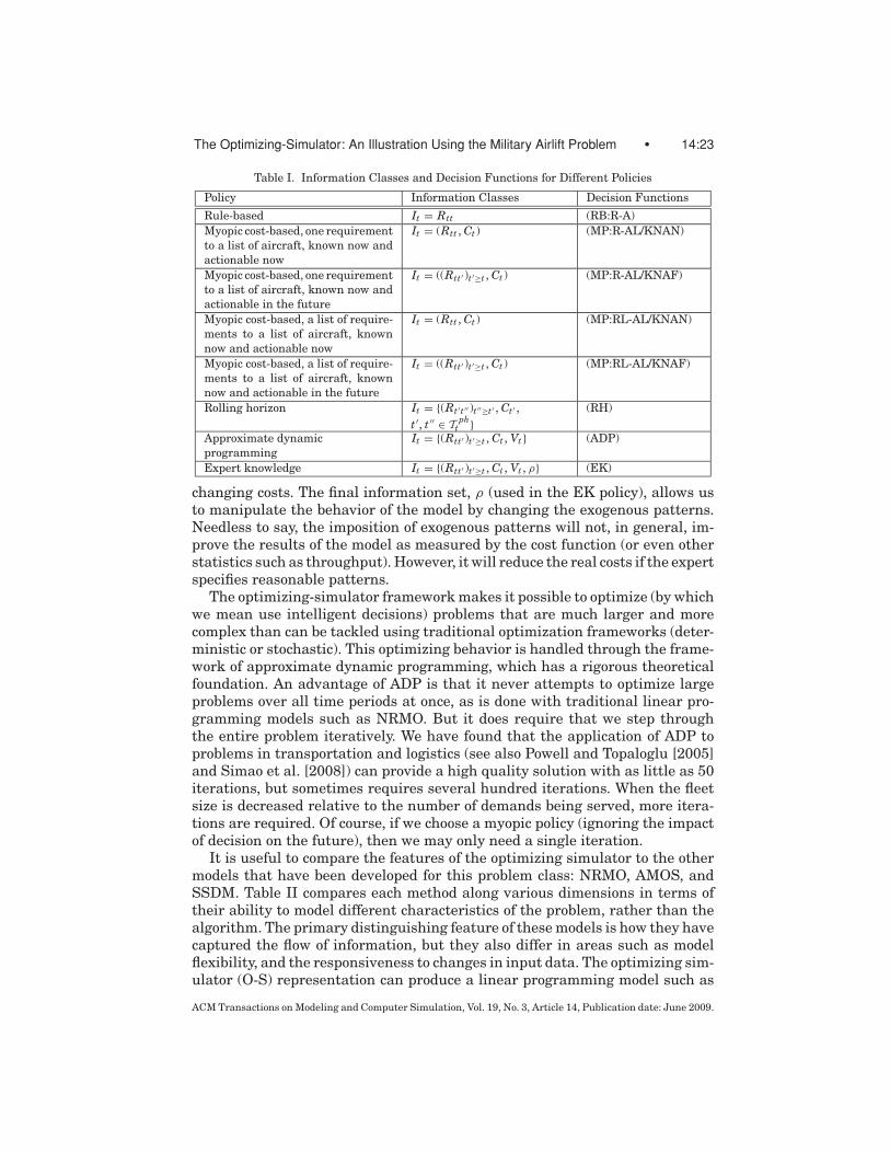
Table I. Information Classes and Decision Functions for Different Policies

Policy Information Classes Decision Functions

Rule-based It = Rtt (RB:R-A)Myopic cost-based, one requirementto a list of aircraft, known now andactionable now

It = (Rtt , Ct ) (MP:R-AL/KNAN)

Myopic cost-based, one requirementto a list of aircraft, known now andactionable in the future

It = ((Rtt′ )t′≥t , Ct ) (MP:R-AL/KNAF)

Myopic cost-based, a list of require-ments to a list of aircraft, knownnow and actionable now

It = (Rtt , Ct ) (MP:RL-AL/KNAN)

Myopic cost-based, a list of require-ments to a list of aircraft, knownnow and actionable in the future

It = ((Rtt′ )t′≥t , Ct ) (MP:RL-AL/KNAF)

Rolling horizon It = {(Rt′t′′ )t′′≥t′ , Ct′ ,t ′, t ′′ ∈ T ph

t }(RH)

Approximate dynamicprogramming

It = {(Rtt′ )t′≥t , Ct , Vt } (ADP)

Expert knowledge It = {(Rtt′ )t′≥t , Ct , Vt , ρ} (EK)

changing costs. The final information set, ρ (used in the EK policy), allows usto manipulate the behavior of the model by changing the exogenous patterns.Needless to say, the imposition of exogenous patterns will not, in general, im-prove the results of the model as measured by the cost function (or even otherstatistics such as throughput). However, it will reduce the real costs if the expertspecifies reasonable patterns.

The optimizing-simulator framework makes it possible to optimize (by whichwe mean use intelligent decisions) problems that are much larger and morecomplex than can be tackled using traditional optimization frameworks (deter-ministic or stochastic). This optimizing behavior is handled through the frame-work of approximate dynamic programming, which has a rigorous theoreticalfoundation. An advantage of ADP is that it never attempts to optimize largeproblems over all time periods at once, as is done with traditional linear pro-gramming models such as NRMO. But it does require that we step throughthe entire problem iteratively. We have found that the application of ADP toproblems in transportation and logistics (see also Powell and Topaloglu [2005]and Simao et al. [2008]) can provide a high quality solution with as little as 50iterations, but sometimes requires several hundred iterations. When the fleetsize is decreased relative to the number of demands being served, more itera-tions are required. Of course, if we choose a myopic policy (ignoring the impactof decision on the future), then we may only need a single iteration.

It is useful to compare the features of the optimizing simulator to the othermodels that have been developed for this problem class: NRMO, AMOS, andSSDM. Table II compares each method along various dimensions in terms oftheir ability to model different characteristics of the problem, rather than thealgorithm. The primary distinguishing feature of these models is how they havecaptured the flow of information, but they also differ in areas such as modelflexibility, and the responsiveness to changes in input data. The optimizing sim-ulator (O-S) representation can produce a linear programming model such as


14:24 • T. T. Wu et al.

Table II. Characteristics of NRMO, AMOS, SSDM and O-S Models

Model NRMO AMOS SSDM O-SCategory Large-scale lin-

ear programmingSimulation Multi-stage

stochasticprogramming

Optimizing-simulator

Informationprocesses

Requiresknowing allinformationwithin T at time0. Cannotdistinguishbetweenknowable time tand actionabletime t ′ ≥ t.

Assumesactionable timeequals knowabletime. May, butdoesn’t,distinguishbetween knowabletime t andactionable timet ′ ≥ t.

Actionable timeequals knowabletime.

Generalmodeling ofknowable andactionabletime. At timet, know theinformationthat isactionable attime t ′ ≥ t.

AttributeSpace

Multi-commodityflow (attributeincludes aircrafttype andlocation)

Multi-attribute(location, fuellevel,maintenance)

Homogeneousships and cargo,extendable tomultiple shiptypes

Generalresource

Complexityof systemdynamics

Linear systemsof equations

Complex systemdynamics

Simple linearsystems ofequations

Complexsystemdynamics

Informationprocess

Deterministic Sequentialinformationprocess

Multiplescenarios

Sequentialinformationprocess

DecisionSelection

Cost-based Rule-based Cost-based Span fromrule-based tocost-based

InformationModeling

Assumes thateverything isknown.

Myopic, localinformation

Assumesknowing theprobabilitydistribution ofscenarios.

Generalmodeling ofinformation

ModelBehavior

Reacts to datachangesintelligently, butnot necessarilyrobustly acrossrandom events.

Noisy response tochanges in inputdata

Similar to LP, butproduces robustallocations.

Can react withintelligence;will displaysome noisecharacteristicof simulation;robust.

Modelingtime

Physicalactivities indiscrete time

Decisions indiscrete time,physical activitiesin continuous time

Physical andinformationprocesses indiscrete time

Decisions indiscrete time,physical andinformationprocesses incontinuoustime



NRMO if we ignore evolving information processes, or a simulation model suchas AMOS, if we explicitly model the TPFDD as an evolving information processand code the appropriate rules for making decisions. As such, the O-S repre-sentation provides a mathematical representation that spans optimization andsimulation.

5. NUMERICAL EXPERIMENTS

We now undertake to demonstrate the spectrum of simulations by showing howincreasing the level of information when we are making a decision improvesthe overall quality of the solution. We undertake these experiments using anunclassified TPFDD dataset for a military airlift problem. The problem is tomanage six aircraft types (C-5A, C-5B, C-17, C-141B, KC-10A, and KC-135) tomove a set of requirements of cargo and passengers between the USA and SaudiArabia, where the total weight of the requirements is about four times the totalcapacities of all the aircraft. In the simulation, a typical delivery trip (pick upplus loaded movement) needs four days to complete, thus all requirements needroughly 16 days to be delivered if the capacities of all the aircraft are used. Thesimulation horizon is 50 days, divided into four hour time intervals. Movinga requirement involves being assigned to a route that will bring the aircraftthrough a series of intermediate airbases for refueling and maintenance. Oneof the biggest operational challenges of these aircraft is that the probability of afailure of sufficient severity to prevent a timely takeoff ranges between 10 and25 percent. A failure can result in a delay or even require an off-loading of thefreight to another aircraft. To make the model interesting, we assume that anaircraft of type C-141B (regardless of whether it is empty or loaded) has a 20percent probability of failure, and needs five days to be repaired if it fails at anairbase in region E (airbase code names starting with E are located primarilyin Northern Europe). All other aircraft types or airbases are assumed to be ableto repair the failures without delay.

The TPFDD file does not capture the time when the information about arequirement becomes known. For our experiments, we assumed that require-ments are known two days before they have to be moved. Aircraft, on the otherhand, are either actionable now (if they are empty and on the ground) or areactionable at the end of a trip that is in progress. We assume that there arethree types of costs involved in the military airlift problem: transportation costs(2 cents per mile per pound of capacity of an aircraft), aircraft repair costs(6 cents per period per pound of capacity of a disabled aircraft) and penaltiesfor late deliveries (4 cents per period per pound of requirement delivered late).

We have such a rich family of models that it would become clumsy if we com-pared all the policies introduced in Section 4. To focus on the main idea of thisarticle, we run the optimizing-simulator on the following policies: (1) rule-based,one requirement to one aircraft (RB:R-A), (2) cost-based, one requirement to alist of aircraft that are knowable now, actionable now (MP:R-AL/KNAN), (3)cost-based, a list of requirements to a list of aircraft that are knowable now,actionable now (MP:RL-AL/KNAN), (4) the same policy but with aircraft thatare knowable now, actionable in the future (MP:RL-AL/KNAF), and (5) the


14:26 • T. T. Wu et al.

Fig. 4. Costs of different policies.

approximate dynamic programming policy (ADP). These five classes shouldprovide improved solutions as they are added. We did not explicitly test rollinghorizon procedures since this would have required generating a forecast of fu-ture events from the TPFDD. This would be straightforward in the context ofa civilian application such as freight transportation where historical activitieswould form the basis of a forecast, but a historical record does not exist for theseapplications.

We use three measures of solution quality. The first is the traditional measureof the objective function. It is important to emphasize that this is an imperfectmeasure, since some behaviors may not be reflected in a cost function. Thesecond measure is throughput, which is of considerable interest in the studyof airlift problems. Our cost function captures throughput indirectly throughcosts that penalize late deliveries. Finally, when we study the use of expertknowledge, we measure the degree to which the model matches exogenouslyspecified patterns.

Figure 4 shows the costs for each of the first five policies. Policy (RB:R-A) isrule-based, one requirement to one aircraft. Policy (MP:R-AL/KNAN) is cost-based, one requirement to a list of aircraft that are knowable now actionablenow. Policy (MP:RL-AL/KNAN) is cost-based, a list of requirements to a list ofaircraft that are knowable now, actionable now. Policy (MP:RL-AL/KNAF) is



Fig. 5. Throughput curves of different policies.

cost-based, a list of requirements to a list of aircraft that are knowable now ac-tionable in the future. Policy (ADP) is the approximate dynamic programmingpolicy. The total cost is the sum of transportation costs, late delivery costs, andaircraft repair costs. The late delivery costs decrease steadily as the informationset increases. The repair cost is significantly reduced in policy (ADP) since thispolicy learns from the early iterations and avoids sending aircraft to airbasesthat lead to longer repair times. However, the detour increases the transporta-tion cost of policy (ADP) slightly compared to policy (MP:RL-AL/KNAF). Theoverall total costs are decreasing as we expected, since the information sets areincreasing.

The throughput of each of the five different policies (RB:R-A), (MP:R-AL/KNAN), (MP:RL-AL/KNAN), (MP:RL-AL/KNAF), and (ADP), are plottedin Figure 5, which shows cumulative pounds delivered over the simulation.Also shown is the cumulative expected throughput curve, which representsthe cumulative total tonnage that has been requested to move. The cumula-tive expected throughput curve assumes that every unit of demand is movedinstantaneously, so this represents the best that the system can do.

The throughput also follows this sequence, from the right to the left. It is clearthat the richer the information class, the faster the delivery—i.e. the closer to


14:28 • T. T. Wu et al.

Table III. Areas Between the CumulativeExpected Throughput Curve and the

Throughput Curves of Different Policies

Policy pounds * day(RB:R-A) 472,868,381(MP:R-AL/KNAN) 344,977,669(MP:RL-AL/KNAN) 303,568,943(MP:RL-AL/KNAF) 281,365,953(ADP) 234,915,133

the left is the throughput curve. Since some of the throughput curves crosseach other, we calculate the area between the expected throughput and thethroughput curves of different policies and list them in Table III. These areasactually measure the lateness of the delivery of different policies. The smallerthe area is, the faster the delivery is. We may see that from policy (RB:R-A) to(ADP), the areas are decreasing from 473 million to 235 million (pound Days).

We tested the inclusion of expert knowledge by using an exogenous patternto control the percentage of C-5As and C-5Bs through region E. Starting withthe best myopic policy (MP:RL-AL/KNAF), we found that C-5As and Bs wentthrough region E 18.5 percent of the time. We then imposed a single exogenouspattern on the (attribute, decision) pair (a = C-5A or C-5B, d = region E).We then varied the exogenous pattern ρad from 0 to 0.5 in steps of 0.10. Forexample, ρad = 0.3, indicates that as recommended by the expert, C-5As andC-5Bs should be sent through region E in 30% of the instances in which adecision is to be applied to them.

Choosing the correct value of the pattern weight, θ , (which determines thedeviation of the final solution from the solution that exactly matches the exoge-nous pattern) is a matter of subjective judgment. If the cost function has beencarefully designed, then some amount of deviation may still be acceptable. Foreach value of ρad , we varied θ over the values 0, 3, 5, 10, 100, 1000.

The results are shown in Figure 6, which maps the observed pattern fromthe model to the expert-recommended pattern. The horizontal line correspondsto θ = 0, and we also show a 45 degree dashed line representing the case thatthe model matches the pattern exactly. For the remaining runs, varying θ fordifferent values of ρad produces a series of lines that are bounded by the no-pattern and the exact-match lines. Note that matching an exogenous patternwill typically produce a lower objective function (or higher costs). The point ofmatching patterns is to produce a behavior that is not captured by the objectivefunction.

These results indicate that we can retain the ability that exists in traditionalsimulators to guide the behavior of the cost model using simple rules. It isimportant to emphasize, however, that our exogenous patterns are restrictedin their complexity. A rule must be a function of the (attribute, decision) pair(a, d ), which means that the rule may not reflect, for example, informationabout other aircraft (the cost model must pick this up).

The point of these experiments is not to conclude that one decision functionis better than another, since the objective function (Figure 4) or throughput(Figure 5) represent only two measures of a solution. It is interesting that as



Fig. 6. Pattern match under different θ weights.

of this writing, the analysis group at the air mobility command continues touse the simplest rule-based logic, even after contracting to have their originalsimulation package completely rewritten.

6. CONCLUSIONS

The modeling community in transportation, and in particular in the area ofairlift modeling, has traditionally been divided between simulation, which of-fers tremendous flexibility as well as the ability to handle uncertainty, andoptimization, which offers high quality solutions but limits our ability to han-dle uncertainty as well as more complex dynamics. These have been viewed ascompeting methodologies, and the communities that promote them have littleoverlap.

We have shown, using the context of modeling cargo movements for militaryoperations, that simulation and optimization can be viewed as different types ofdecision functions using different types of information. Decision functions canbe rule-based or cost-based, and we illustrate them by showing how differenttypes of functions can be created using four classes of information. While thereis a desire, especially in the academic community, to find the best solution (or thebest policy), it is often the case that in practice the goal is a model that mimicsactual operations. This means not only modeling the physics of the problem(travel times, capacities and constraints), but also the way that decisions aremade. A major limitation that has often been cited by the analysis group at theairlift mobility command is that optimization models are “too smart.”


14:30 • T. T. Wu et al.

For the airlift problem we considered, we showed that increasing the infor-mation available to a decision-maker improves the solution quality in terms ofspecific metrics. However, the logic anticipates that there may be issues we arenot capturing, and we show how we can design decision functions that allowan analyst to guide the model using explicit patterns of behavior. These pat-terns are expressed as a form of goal, rather than the hard rules that are morecommon in simulation models.

The academic literature has focused on finding the best decision (for deter-ministic problems) or the best policy (for stochastic problems). We suggest that anew line of research falls in the area of model calibration. Companies who wantto use these models to answer high-level policy questions gain confidence whenthey feel that the model closely matches the performance of their operation.For civilian operations, historical data may be available, introducing the newchallenge of designing procedures that produce the best match by manipulat-ing the policy. This article shows that by controlling the available information,we can create a broad range of policies, including those that directly competewith optimization models. An interesting research challenge would be to createautomated procedures that identify the policies that produce the closest matchbetween model and history.

ACKNOWLEDGMENTS

The authors gratefully acknowledge the very helpful comments of the referees.

REFERENCES

BAKER, S., MORTON, D., ROSENTHAL, R., AND WILLIAMS, L. 2002. Optimizing military airlift. Oper.Res. 50, 4, 582–602.

BERTSEKAS, D. AND TSITSIKLIS, J. 1996. Neuro-Dynamic Programming. Athena Scientific, Belmont.BROOKE, A., KENDRICK, D., AND MEERAUS, A. 1992. GAMS: A User’s Guide, 2.25 ed. Duxbury

Press/Wadsworth Publishing Company, Belmont.BURKE, J. F., LOVE, R. J., AND MACAL, C. M. 2004. Modelling force deployments from army installa-

tions using the transportation system capability (TRANSCAP) model: A standardized approach.Math. Comput. Model. 39, 6-8, 733–744.

CRAINIC, T. AND GENDREAU, M. 2002. Cooperative parallel tabu search for capacitated networkdesign. J. Heuristics 8, 6, 601–627.

CRINO, J. R., MOORE, J. T., BARNES, J. W., AND NANRY, W. P. 2004. Solving the theater distribu-tion vehicle routing and scheduling problem using group theoretic tabu search. Math. Comput.Model. 39, 6-8, 599–616.

DANTZIG, G. AND FERGUSON, A. 1956. The allocation of aircraft to routes: An example of linearprogramming under uncertain demand. Manage. Sci. 3, 45–73.

FERGUSON, A. AND DANTZIG, G. B. 1955. The problem of routing aircraft—a mathematical solution.Aeronaut. Eng. Rev. 14, 51–55.

FU, M. 2002. Optimization for simulation: Theory vs. practice. INFORMS J. Comput. 14, 3, 192–215.

GODFREY, G. AND POWELL, W. B. 2002. An adaptive, dynamic programming algorithm forstochastic resource allocation problems I: Single period travel times. Transport. Sci. 36, 1,21–39.

GOGGINS, D. A. 1995. Stochastic modeling for airlift mobility. M.S. thesis, Naval PostgraduateSchool, Monterey.



GRANGER, J., KRISHNAMURTHY, A., AND ROBINSON, S. M. 2001. Stochastic modeling of airlift opera-tions. In Proceedings of the 2001 Winter Simulation Conference, B. A. Peters, J. S. Smith, D. J.Medeiros, and M. W. Rohrer, Eds. 432–440.

JUDD, K. 1998. Numerical Methods in Economics. MIT Press.KILLINGSWORTH, P. AND MELODY, L. J. 1997. Should C17’s be deployed as theater assets?: An appli-

cation of the CONOP air mobility model. Tech. Rep. rand/db-171-af/osd, Rand Corporation.MARAR, A. AND POWELL, W. B. 2002. Using static flow patterns in time-staged resource allocation

problems. Tech. Rep., Princeton University, Department of Operations Research and FinancialEngineering.

MATTOCK, M. G., SCHANK, J. F., STUCKER, J. P., AND ROTHENBERG, J. 1995. New capabilities forstrategic mobility analysis using mathematical programming. Tech. Rep., RAND Corporation.

MIDLER, J. L. AND WOLLMER, R. D. 1969. Stochastic programming models for airlift operations.Nav. Res. Logist. Quart. 16, 315–330.

MORTON, D. P., ROSENTHAL, R. E., AND LIM, T. W. 1996. Optimization modeling for airlift mobility.Mil. Oper. Res. 49–67.

MORTON, D. P., SALMERON, J., AND WOOD, R. K. 2002. A stochastic program for optimizing militarysealift subject to attack. Stochastic Programming e-Print Series, http://www.speps.info.

NIEMI, A. 2000. Stochastic Modeling for the NPS/RAND Mobility Optimization Model. Depart-ment of Industrial Engineering, University of Wisconsin-Madison,http://ie.engr.wisc.edu/robinson/Niemi.htm.

POWELL, W. B. 2007. Approximate Dynamic Programming: Solving the Curses of Dimensionality.John Wiley and Sons, New York.

POWELL, W. B. AND TOPALOGLU, H. 2005. Fleet management. Applications of Stochastic Program-ming, S. Wallace and W. Ziemba, Eds. Math Programming Society—SIAM Series in Optimization,Philadelphia.

PUTERMAN, M. L. 1994. Markov Decision Processes. John Wiley & Sons, New York.ROSENTHAL, R., MORTON, D., BAKER, S., LIM, T., FULLER, D., GOGGINS, D., TOY, A., TURKER, Y., HORTON,

D., AND BRIAND, D. 1997. Application and extension of the Thruput II optimization model forairlift mobility. Mil. Oper. Res. 3, 2, 55–74.

SCHANK, J., MATTOCK, M., SUMNER, G., GREENBERG, I., AND ROTHENBERG, J. 1991. A review of strategicmobility models and analysis. Tech. Rep., RAND Corporation.

SIMAO, H. P., DAY, J., GEORGE, A. P., GIFFORD, T., NIENOW, J., AND POWELL, W. B. 2008. An approximatedynamic programming algorithm for large-scale fleet management: A case application. Transport.Sci. 43, 2, 178–197.

SPIVEY, M. AND POWELL, W. B. 2004. The dynamic assignment problem. Transport. Sci. 38, 4,399–419.

STUCKER, J. P. AND BERG, R. T. 1999. Understanding airfield capacity for airlift operations. Tech.Rep., RAND Corporation.

SWISHER, J., JACOBSON, S., AND YUCESAN, E. 2003. Discrete-event simulation optimization usingranking, selection, and multiple comparison procedures: A survey. ACM Trans. Model. Comput.Simul. 13, 2, 134–154.

TOPALOGLU, H. AND POWELL, W. B. 2002. Dynamic programming approximations for stochastic,time-staged integer multicommodity flow problems. Tech. Rep., Princeton University, Depart-ment of Operations Research and Financial Engineering.

TSITSIKLIS, J. N. AND VAN ROY, B. 1996. Feature-based methods for large scale dynamic program-ming. Mach. Learn. 22, 59–94.

WING, V., RICE, R. E., SHERWOOD, R., AND ROSENTHAL, R. E. 1991. Determining the optimal mobilitymix. Tech. Rep., Force Design Division, The Pentagon, Washington D.C.

YOST, K. A. 1994. The thruput strategic airlift flow optimization model. Tech. Rep., Air ForceStudies and Analyses Agency, The Pentagon, Washington D.C.

YOST, K. A. AND WASHBURN, A. R. 2000. The LP/POMDP marriage: Optimization with imperfectinformation. Nav. Res. Logist. 47, 8, 607–619.

Received July 2008; revised September 2008; accepted October 2008


Documents

The optimizing-simulator: An illustration using the military airlift problem