Embed Size (px)
Citation preview
-i-
The optimisation of GC x GC and the analysis of diesel
petrochemical samples
by
Werner Welthagen
Submitted in partial fulfilment of
the requirements for the degree of
Master of Science (Chemistry)
In the Faculty of Natural and Agricultural Sciences
University of Pretoria
UUnniivveerrssiittyy ooff PPrreettoorriiaa eettdd –– WWeelltthhaaggeenn WW ((22000055))

-ii-
Acknowledgments
I wish to thank my promoter, Prof E. R. Rohwer, for his patient guidance, encouragement and
support.
A thanks to all my co-workers that chipped in with useful information and hints to achieve my final
goals. In particular to Tony Hasset, Erla Harden and Andre Venter. A word of thanks also to David
Masemula who kept my nitrogen bottles full.
I would like to thank SASOL for supporting and funding this project.
Finally a thanks to all my friends and family who kept my motivation going and supported me in
and outside of the lab.
UUnniivveerrssiittyy ooff PPrreettoorriiaa eettdd –– WWeelltthhaaggeenn WW ((22000055))
-iii-
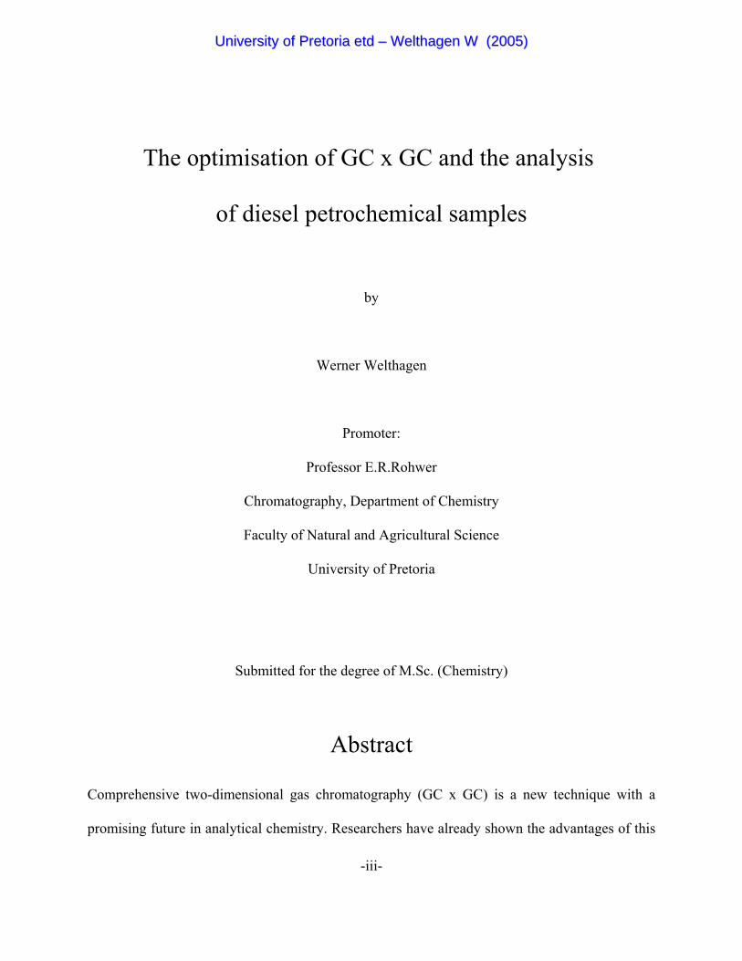
The optimisation of GC x GC and the analysis
of diesel petrochemical samples
by
Werner Welthagen
Promoter:
Professor E.R.Rohwer
Chromatography, Department of Chemistry
Faculty of Natural and Agricultural Science
University of Pretoria
Submitted for the degree of M.Sc. (Chemistry)
Abstract
Comprehensive two-dimensional gas chromatography (GC x GC) is a new technique with a
promising future in analytical chemistry. Researchers have already shown the advantages of this
UUnniivveerrssiittyy ooff PPrreettoorriiaa eettdd –– WWeelltthhaaggeenn WW ((22000055))
-iv-
technique to unravel complex samples consisting of hundreds of compounds. The predominant
advantage of GC x GC above conventional one-dimensional gas chromatography is the greatly
enhanced peak capacity. To fully utilise this enhanced peak capacity the instrumentation needs to
be run at optimum conditions. The optimisation of one-dimensional gas chromatography (GC) is
done on a routine basis in analytical laboratories and handbooks are available to cover these
optimisation strategies. This study was aimed at providing similar guidelines for GC x GC. Since
the underlying theory of GC and GC x GC are essentially the same, conventional GC optimisation
strategies were the point of departure for this research. The different operational parameters in GC
x GC were identified and emphasis was then placed on a method to simultaneously optimise the flow
rate in both columns, taking into consideration the common practice of series-coupling of columns
of different internal diameters. The influence of second-dimension stationary phase, temperature
program and modulator operation on the distribution and shape of chromatographic peaks in the two
dimensions is also investigated. The results obtained from this study provide a useful new approach
to optimise a GC x GC system where two gas chromatographic columns of various dimensions are
connected in series. The use of diesel samples in this optimisation process presented some useful
applications for future research in the petrochemical industry. Examples of potential applications
such as “fingerprinting techniques” and compositional analysis are also discussed.
UUnniivveerrssiittyy ooff PPrreettoorriiaa eettdd –– WWeelltthhaaggeenn WW ((22000055))
-v-
The optimisation of GC x GC and the analysis
of diesel petrochemical samples
(Die optimering van GC x GC en die analise
van diesel petrochemiese monsters)
deur
Werner Welthagen
Promotor:
Professor E.R.Rohwer
Chromatografie, Departement Chemie
Fakulteit van Natuur- en Landbouwetenskappe
Universiteit van Pretoria
Voorgelê vir die graad M.Sc. (Chemie)
Ekserp
Twee-dimensionele gaschromatografie (GC x GC) is ‘n nuwe tegniek met ‘n belowende toekoms
in analitiese chemie. Navorsers het reeds die voordele van die tegniek uitgewys om komplekse
UUnniivveerrssiittyy ooff PPrreettoorriiaa eettdd –– WWeelltthhaaggeenn WW ((22000055))
-vi-
monsters, bestaande uit honderde komponente, te ontrafel. Die mees prominente voordeel van GC
x GC bo gewone een-dimensionele GC is die verhoogde piek-kapasiteit. Om die groter piek-
kapasiteit ten volle te benut moet die instrument by optimum kondisies funksioneer. Die optimering
van een-dimensionele GC word gedoen op ‘n roetinebasis in menigte analitiese laboratoriums en
daar is handboeke beskikbaar wat die optimering van GC bespreek. Hierdie studie was daarop
gemik om soortgelyke riglyne vir die optimering van die meer komplekse GC x GC daar te stel.
Omdat die onderliggende teorie van GC en GC x GC essensieel dieselfde is, is konvensionele GC-
optimering gebruik as uitgangspunt gebruik vir hierdie navorsing. Die verskillende operasionele
parameters in GC x GC is eers geïdentifiseer, waarna klem gelê is op ‘n metode wat gelyktydig die
lineêre vloei in beide kolomme kan optimeer, met inagneming van die algemene praktyk om serie-
gekoppelde kolomme met verskillende binnedeursneë te gebruik. Die invloed van die tweede-
dimensie stasionêre fase, temperatuur-programmering en die modulator op die vorm en verspreiding
van chromatografiese pieke in die twee dimensies is ook ondersoek. Die resultate verkry in hierdie
studie bevestig die bruikbaarheid van ‘n nuwe optimeringsmetode vir GC x GC waar kolomme van
verskillende binnedeursnit aanmekaar gekoppel word. Die gebruik van dieselmonsters in die
optimeringstudie het ‘n paar potensiële gebruike uitgewys vir toekomstige navorsing in die
petrochemiese industrie. Voorbeelde bespreek sluit hoofkomponent- en “vingerafdruk”- analises
in.
UUnniivveerrssiittyy ooff PPrreettoorriiaa eettdd –– WWeelltthhaaggeenn WW ((22000055))
-vii-
Contents
Acknowledgments ii
Abstract iii
Ekserp v
List of tables xi
List of figures xii
1 Introduction 1
1.1 Background 1
1.2 Approach 3
1.3 Presentation and arrangement 4
2 Background: Part 1
GC x GC as a multidimensional technique 6
2.1 Multidimensional separation techniques 7
2.2 Principles of comprehensively coupled techniques 9
2.2.1 Comprehensive coupling 9
2.2.2 Peak capacity 10
2.2.3 Orthogonality 10
2.2.4 Modulation 11
UUnniivveerrssiittyy ooff PPrreettoorriiaa eettdd –– WWeelltthhaaggeenn WW ((22000055))
-viii-
2.3 GC x GC 11
2.3.1 Definition 11
2.3.2 Modulators in GC x GC 12
2.3.2.1 Thermal modulation 14
2.3.2.2 Cryofocussing modulation 16
2.3.2.3 Diaphragm-valve modulation 21
2.3.2.4 Comparison of Modulators 21
2.3.3 Detectors in GC x GC 23
2.3.4 Interpretation of GC x GC separation 23
2.3.5 GC x GC vs GC - GC 25
3 Background: Part 2
GC x GC optimisation 26
3.1 Introduction 27
3.2 One dimensional GC considerations 28
3.2.1 Column stationary phase 28
3.2.2 Column dimensions 30
3.2.3 Linear flow rate 31
3.2.4 Temperature considerations 32
3.2.5 Fast isothermal GC 33
3.2.6 Injection techniques 35
3.3 Combining the two columns 35
3.4 Conclusions 36
UUnniivveerrssiittyy ooff PPrreettoorriiaa eettdd –– WWeelltthhaaggeenn WW ((22000055))
-ix-
4 Background: Part 3
The analysis of petrochemical samples 37
4.1 Introduction 38
4.2 Gas Chromatography (GC) 38
4.2.1 Simulated distillation (SimDist) 39
4.2.2 PIONA analysis 40
4.3 GC x Selective Detector 40
4.4 GC x GC 41
4.5 GC x GC x Selective Detector 41
4.6 Other applications of GC x GC 42
2.6.1 Fast screening 42
2.6.2 Environmental samples 42
4.7 Conclusions 43
5 Optimisation of GC x GC parameters 44
5.1 Introduction 45
5.2 General experimental setup 46
5.2.1 Instrumentation 46
5.2.2 Computer software 47
5.2.2.1 Operating software 47
5.2.2.2 Data acquisition software 47
5.2.2.3 Data analysis and visualisation 48
5.2.3 Samples used 49
UUnniivveerrssiittyy ooff PPrreettoorriiaa eettdd –– WWeelltthhaaggeenn WW ((22000055))
-x-
5.3 Optimising the column parameters 49
5.3.1 Linear flow rates 50
5.3.2 Optimisation of the flow rates for optimum
resolution 52
5.3.3 Choice of second dimension stationary phase 68
5.3.4 Temperature difference between columns 75
5.4 Modulator optimisation 76
6 Analysis of diesel petroleum fractions 80
6.1 Introduction 81
6.2 Experimental setup 82
6.3 The analysis of four local diesel samples 83
6.4 The analysis of diesel-paraffin mixtures 95
7 Conclusion 103
7.1 Optimisation of GC x GC 104
7.2 The analysis of diesel petrochemical samples 107
References 108
Appendix A Software created for data handling 116
Appendix B Calculations 126
UUnniivveerrssiittyy ooff PPrreettoorriiaa eettdd –– WWeelltthhaaggeenn WW ((22000055))
-xi-
List of Tables
Table 1 One-dimensional separations which might serve as building
blocks for multidimensional separation techniques [1] 8
Table 2 Comparison of modulators [15] 22
Table 3 Different non-polar stationary phases [24] 29
Table 4 Second-dimension polar stationary phases [24] 30
Table 5 Inlet pressures corresponding to the average linear flow rates
in the first- and second-dimension 55
Table 6 The k - values and k - term used in the resolution equation 61
Table 7 The % - values and % - term used in the resolution equation 61
Table 8 Names of peaks used in the diesel and paraffin chromatograms 74
UUnniivveerrssiittyy ooff PPrreettoorriiaa eettdd –– WWeelltthhaaggeenn WW ((22000055))
-xii-
Figure 1 Slotted thermal heater developed by Phillips [8] 14
Figure 2 The two different resistively heated modulators, (A) is designed by
Philips et al [4] and (B) designed by Burger et al [9] 15
Figure 3 Longitudinal modulator developed by Marriot [12] 16
Figure 4 The trap assembly of the LMCS [12] 17
Figure 5 The single-jet thermal modulator by Ledford[9] 18
Figure 6 Nitrogen cryogenic thermal modulator with four jets developed
by Ledford [13] 19
Figure 7 Duel stage jet modulator of Beens and co workers [14] 20
Figure 8 Schematic diagram of a diaphragm-valve modulator by Synovec [10] 21
Figure 9 Influence of Linear flow rate, u, on peak broadening during
chromatographic separation (Efficiency) measured as HETP [27] 31
UUnniivveerrssiittyy ooff PPrreettoorriiaa eettdd –– WWeelltthhaaggeenn WW ((22000055))
-xiii-
Figure 10 The graph of k /(k+1) against k [23] 33
Figure 11 The change in the Van Deemter curve with change in column
inner diameter [31] 34
Figure 12 Graphical representation of the optimisation strategy with GC x GC
peaks eluting at about 25EC from a diesel sample. 54
Figure 13 Resolution plotted against the linear flow rate of the first-dimension
at different inlet pressures. 56
Figure 14 Resolution plotted against the linear flow rate of the second-dimension
at different inlet pressures. 57
Figure 15 Plot of resolution of the first- and second-dimension against the
system inlet pressure (the absolute resolution values of the second-dimension
is adjusted by a factor of 3.2 for better visual comparison). 58
Figure 16 The plot of the square root of the plate number (N) against the inlet
head pressure for the evaluating the k- and α-term dependency of the resolution
optimisation method. 63
Figure 17 The plate height for both of the two peaks used in the resolution
calculations is calculated and plotted against the linear velocity of
the second-dimension to give Van Deemter plots of the
second-dimension. 64
UUnniivveerrssiittyy ooff PPrreettoorriiaa eettdd –– WWeelltthhaaggeenn WW ((22000055))
-xiv-
Figure 18 A comparison between diesel chromatograms using the generally
accepted linear flow rate of 40 cm/s for the first-dimension and the
optimised linear flow rate of 22 cm/s 67
Figure 19a The chromatogram of a diesel sample analysed on a PEG second-
dimension column 70
Figure 19b The chromatogram of a diesel sample analysed on a cyano-
propylphenyl second- dimension column 72
Figure 20 The peaks circled in red on the left of the picture represent second-
dimension eluents that overlap with those of the next second-dimension
run. This phenomenon is called “wrap-around” 76
Figure 21 Actual peak profiles obtained with adjustment of the heat pulses,
top figure indicating a good peak shape (60-180 ms heat pulse), the
middle one a too short heat pulse (smaller than 60 ms)and the last
one a too long heat pulse (longer than 180 ms). 77
Figure 22a A one-dimensional chromatogram of a Total diesel sample 84
Figure 22b A one-dimensional chromatogram of a BP diesel Sample 84
Figure 22c A one-dimensional chromatogram of a Shell diesel sample 85
Figure 22d A one-dimensional chromatogram of a SASOL diesel sample 85
UUnniivveerrssiittyy ooff PPrreettoorriiaa eettdd –– WWeelltthhaaggeenn WW ((22000055))
-xv-
Figure 23a A two-dimensional chromatogram of a Total diesel sample 87
Figure 23b A two-dimensional chromatogram of a BP diesel sample 89
Figure 23c A two-dimensional chromatogram of a Shell diesel sample 91
Figure 23d A two-dimensional chromatogram of a SASOL diesel sample 93
Figure 24a A two-dimensional chromatogram of a 100% paraffin sample 98
Figure 24b A two-dimensional chromatogram of a 33% diesel 66% paraffin mixture 99
Figure 24c A two-dimensional chromatogram of a 1:1 diesel : paraffin mixture 100
Figure 24d A two-dimensional chromatogram of a 66% diesel 33% paraffin mixture 101
Figure 24e A two-dimensional chromatogram of a 100% diesel sample 102
UUnniivveerrssiittyy ooff PPrreettoorriiaa eettdd –– WWeelltthhaaggeenn WW ((22000055))

-1-
Chapter 1
Introduction
Table of Contents
1.1 Background
1.2 Approach
1.3 Presentation and arrangement
UUnniivveerrssiittyy ooff PPrreettoorriiaa eettdd –– WWeelltthhaaggeenn WW ((22000055))
-2-
Chapter 1
Introduction
1.1 Background
In the ever advancing age of technology the need to improve and control fuels, foods and various
other products is having a more and more integrate part of daily work. Health and other control
organisations are increasing pressure on industries to provide detailed analysis of their products.
Many of the analytical methods used to date can provide good results but at an increasingly high
cost. To achieve most of the regulatory detection levels, these instruments are pushed to their limits,
requiring a support infrastructure and highly skilled manpower that can only be afford by the
developed world. Developing countries find it increasingly difficult to certify their products for
export and domestic use. This is already resulting in some of the countries denouncing products
from these poorer countries.
Some examples:
Automobile fuels need to be carefully controlled to prevent the release of harmful exhaust gases to
the atmosphere. The fuels should not only be less harmful, but also more effective, economic etc.
To achieve these qualities, the composition of the fuel and the function of each of the components
needs to be known and carefully studied.
All products for human consumption have to be monitored carefully. Fresh fruits and other farm
grown products usually contain a variety of potentially harmful pesticides that need to be controlled.
Health organisations across the developed world put a lot of pressure onto the developing countries
to provide food low in pesticide levels. Each of the pesticides used now has a maximum allowed
level in the food, but unfortunately most of these pesticides are complex mixtures and very difficult
to detect, especially in the trace amounts found in food. The food itself contains hundreds of
UUnniivveerrssiittyy ooff PPrreettoorriiaa eettdd –– WWeelltthhaaggeenn WW ((22000055))
-3-
compounds that will mask these pesticides in most analytical techniques used today.
In forensic science, food adulteration analysis, pollution control and in various molecular
fingerprinting techniques, the need to analyse lower levels with greater confidence is also
increasing. Most of the fingerprinting techniques used today are already well established but as
criminals become more and more sophisticated, these techniques become less effective. Arson and
horse-doping serves as examples. The same trend can also be seen in food adulteration; To gain
higher profits many additives have been added to, for example, olive oil that does not influence the
taste but increases the volume. These adulterations have been going on for ages, but the
sophistication in this type of crime has made it increasingly difficult to detect by conventional
methods.
From the above examples it should be clear that there is a critical need for improvements in
complex sample analysis.
One way of improving existing techniques is to couple various instruments to one another for
multidimensional analysis, as discussed in chapter 2. These techniques have already expanded the
scope of analytical chemistry tremendously. The multidimensional technique used in this study is
GC x GC. This instrument uses two gas chromatographic (GC) systems that separate compounds
on the basis of two different molecular properties, for example boiling point and polarity. The two
gas chromatographic systems are coupled in such a way that all the eluent from the first system is
subjected for analysis in the second GC without losing the separation obtained by the first. This is
called comprehensive two-dimensional gas chromatography and will also be discussed in more
detail in chapter 2.
1.2 Approach
Gas chromatography is a well-used technique for various applications. In many of these applications
a level of sophistication has been reached that makes any further improvements on the respective
UUnniivveerrssiittyy ooff PPrreettoorriiaa eettdd –– WWeelltthhaaggeenn WW ((22000055))
-4-
systems too expensive to consider. With the development of the two-dimensional gas
chromatograph (GC x GC) some of these existing applications can be revisited and improvements
can be done at little extra costs. In some cases even a reduction in cost of the current analytical
system can be anticipated.
The focus of this study was to improve techniques used for the analysis of diesel petrochemical
samples. Some of the present techniques in industry, like the PIONA analysis (chapter 4), where
petrochemical fractions are separated into chemical groups, can be potentially replaced by a less
complicated GC x GC system. The GC x GC would also be able to do the same group analysis in
a single run, resulting in significant saving of time and money. Some other applications include
“fingerprinting” of diesel samples and the investigation of interesting properties observed in diesel-
paraffin mixtures used in underground mining operations to decrease exhaust emmisions.
These applications, however, cannot commence before the new technique is fully understood and
can be routinely operated at its maximum potential. Most of this study was thus focussed on
optimising the GC x GC. The optimisation of an analytical instrument, as discussed later in chapter
3, is a prerequisite for reliable analysis. Due to the absence of a guideline for GC x GC
optimisation, the first aim of this study was to create such a guide and to investigate the parameters
involved in optimising the separation efficiency of the instrument.
1.3 Presentation and arrangement
This chapter gives a brief introduction to the background and approach of the work done. In the next
three chapters a background (literature overview) is given of the technique under investigation. In
part 1 of the background the principles of multidimensional techniques are discussed along with the
history and advantages of GC x GC. Part 2 focuses on the optimisation of gas chromatographic
systems and includes the difficulties involved in optimising a comprehensively coupled column
system, such as in GC x GC. Part 3 focusses on the analysis of petrochemical samples, an overview
of the chromatographic methods used today and the potential of employing GC x GC in these fields.
UUnniivveerrssiittyy ooff PPrreettoorriiaa eettdd –– WWeelltthhaaggeenn WW ((22000055))

-5-
Chapter 5 deals with the actual optimisation. Chapter 6 contains some examples of diesel analysis
and in chapter 7 the conclusions are reported.
UUnniivveerrssiittyy ooff PPrreettoorriiaa eettdd –– WWeelltthhaaggeenn WW ((22000055))
-6-
Chapter 2
Background: Part 1
GC x GC as a Multidimensional Technique
Table of Contents
2.1 Multidimensional separation techniques
2.2 Principles of comprehensively coupled techniques
2.2.1 Comprehensive coupling
2.2.2 Peak capacity
2.2.3 Orthogonality
2.2.4 Modulation
2.3 GC x GC
2.3.1 Definition
2.3.2 Modulators in GC x GC2.3.2.1 Thermal modulation
2.3.2.2 Cryofocussing modulation
2.3.2.3 Diaphragm-valve modulation
2.3.2.4 Comparison of Modulators
2.3.3 Detectors in GC x GC
2.3.4 Interpretation of GC x GC separation
2.3.5 GC x GC vs GC - GC
UUnniivveerrssiittyy ooff PPrreettoorriiaa eettdd –– WWeelltthhaaggeenn WW ((22000055))
-7-
Chapter 2
Background: Part 1
GC x GC as a Multidimensional Technique
2.1 Multidimensional separation techniques
The search for answers in complex chemical mixtures, such as the intrinsic lubricating properties
of diesel fuel, demand more detailed separation and analysis. One-dimensional techniques have been
pushed to their limits (in search of these answers) and modern research has therefore been forced
to change the approach to these problems. One strategy has been the introduction of
multidimensional techniques. These techniques are now starting to mature and are slowly filling the
information gaps left by one-dimensional techniques. More complex samples can now be separated
and analysed to answer the questions of every applied scientist: “Why? What? How?”
In multidimensional separation, two or more independent separation techniques are coupled to give
improved resolution and therefore a clearer picture of a sample composition. Such a system utilises
the specific separation parameters of each technique to provide a better, more complete separation
of an extremely complex mixture. Separation parameters are based on characteristic properties of
compounds, such as their partition coefficients or density. There are numerous separation systems,
each using a different property to control separation, each answering a different question. A short
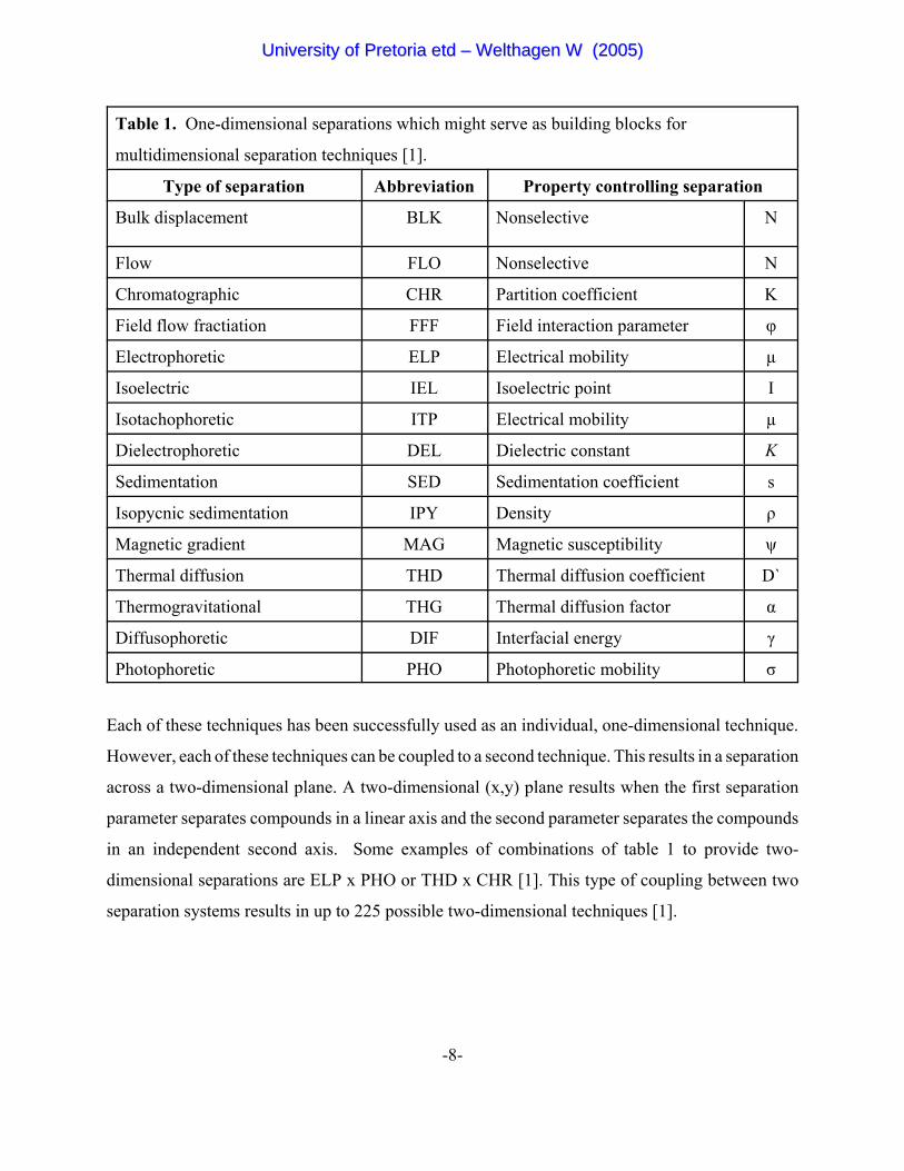
selection of the most common separation types is listed in table 1 [1].
UUnniivveerrssiittyy ooff PPrreettoorriiaa eettdd –– WWeelltthhaaggeenn WW ((22000055))
-8-
Table 1. One-dimensional separations which might serve as building blocks for
multidimensional separation techniques [1].
Type of separation Abbreviation Property controlling separation
Bulk displacement BLK Nonselective N
Flow FLO Nonselective N
Chromatographic CHR Partition coefficient K
Field flow fractiation FFF Field interaction parameter φ
Electrophoretic ELP Electrical mobility µ
Isoelectric IEL Isoelectric point I
Isotachophoretic ITP Electrical mobility µ
Dielectrophoretic DEL Dielectric constant K
Sedimentation SED Sedimentation coefficient s
Isopycnic sedimentation IPY Density ρ
Magnetic gradient MAG Magnetic susceptibility ψ
Thermal diffusion THD Thermal diffusion coefficient D`
Thermogravitational THG Thermal diffusion factor α
Diffusophoretic DIF Interfacial energy γ
Photophoretic PHO Photophoretic mobility σ
Each of these techniques has been successfully used as an individual, one-dimensional technique.
However, each of these techniques can be coupled to a second technique. This results in a separation
across a two-dimensional plane. A two-dimensional (x,y) plane results when the first separation
parameter separates compounds in a linear axis and the second parameter separates the compounds
in an independent second axis. Some examples of combinations of table 1 to provide two-
dimensional separations are ELP x PHO or THD x CHR [1]. This type of coupling between two
separation systems results in up to 225 possible two-dimensional techniques [1].
UUnniivveerrssiittyy ooff PPrreettoorriiaa eettdd –– WWeelltthhaaggeenn WW ((22000055))
-9-
Furthermore, within any single type of separation in table 1, such as chromatography, several
independent, techniques can exist, yielding more coupling options. The following is a list of the
main chromatographic separation techniques.
• Gas liquid chromatography (GLC)
• Gas solid chromatography (GSC)
• Supercritical fluid chromatography (SFC)
• Reverse phase liquid chromatography (RP LC)
• Normal phase liquid chromatography (NP LC)
• Size exclusion liquid chromatography (SE LC)
• Gradient elution liquid chromatography (GE LC)
• Thin layer liquid chromatography (TLC)
Any two of these chromatographic techniques can be coupled to one another to provide some 81
additional two-dimensional separation systems [1]. By adding more parameters to an existing two-
dimensional system, separation would be further enhanced, but it would also increase the complexity
of the system.
2.2 Principles of comprehensively coupled techniques
In order to understand the principles of comprehensively coupled techniques, it is necessary to
examine the associated terminology. The terms of comprehensive coupling, orthogonality, peak
capacity and modulation are discussed in the following sections.
2.2.1 Comprehensive coupling
Comprehensive coupling of two separation techniques is obtained if they are coupled (typically in-
line) to one another in such a way that every single compound subjected to the first separation is
transferred to the second dimension and that the full separation of each technique is preserved.
UUnniivveerrssiittyy ooff PPrreettoorriiaa eettdd –– WWeelltthhaaggeenn WW ((22000055))
-10-
2.2.2 Peak capacity (n)
The effectiveness of most separations is measured by its peak capacity, which is defined as the
maximum number of peaks or zones that will fit into the available separation space [2]. Guiochon
[3] described the enhancement of peak capacity in chromatographic systems. From his work, it can
be deduced that the maximum peak capacity of a two-dimensional system is described
approximately by the multiplicative law.
n2 ~ ny x nz ~ n12
Where n2 represents the peak capacity of the two-dimensional system and obtained by
comprehensively coupling of the two distinct one-dimensional separations of peak capacity ny and
nz. A peak capacity of nl2 is obtained for the special case when ny = nz = nl.
2.2.3 Orthogonality
In order to get separation in a two-dimensional system, two separation parameters are required. The
parameters should be mutually independent to separate compounds over the full separation plane
created by the coupled technique. One such a system is the GC x GC, discussed in section 2.3 in
detail, where the first dimension separates components on a volatility basis according to boiling
point, while the second dimension separates the components further on a polarity basis, giving a
two-dimensional chromatogram with independent axes. Orthogonality thus simply indicates that the
two separation systems are totally independent of each another. For closely related separation
mechanisms, the components of a mixture will tend to elute on the diagonal between the two
separation axes, i.e. again in a single dimension.
UUnniivveerrssiittyy ooff PPrreettoorriiaa eettdd –– WWeelltthhaaggeenn WW ((22000055))
-11-
2.2.4 Modulation
The process of collecting narrow elution fractions from the first separation system and transferring
them to the second is called modulation. To achieve comprehensive coupling of two techniques, the
modulation frequency has to be high enough as to prevent loss of first dimension (D1) separation.
This in turn, limits the time available to the second dimension (D2) separation, as successive
separations have to be performed at the same frequency. The time interval between successive
second dimension injections is known as the modulation period.
2.3 GC x GC
2.3.1 Definition
The abbreviation GC x GC [4] is used when two GCs are connected in a comprehensive orthogonal
manner. This means that two columns are coupled in-line comprehensively so that the separation
in each column is preserved.
Most GC x GC separations start with a non-polar column, where compounds are separated according
to volatility parameters and the second column uses selective molecular interactions (polar or
structural interactions) to separate the compounds further. Gas chromatographic interaction is
dependent on temperature, thus, although the second dimension is based on steric interactions, it still
exhibits strong temperature dependency, resulting in the two dimensions not being completely
orthogonal to each other. This problem can be solved by running the second column at temperatures
close to the elution temperatures of compounds from the first column.
There are four major advantages to GC x GC [5,6,7]
• It provides highly detailed, interpretable images of complex samples
• Peaks can be grouped to represent different chemical classes, creating a viable alternative
for group types analysis.
UUnniivveerrssiittyy ooff PPrreettoorriiaa eettdd –– WWeelltthhaaggeenn WW ((22000055))
-12-
• It provides superior resolution, high peak capacity and increased sensitivity relative to
conventional GC, which allows accurate determination of different components
• It can provide boiling-point distribution for different classes of compounds in one run.
2.3.2 Modulators in GC x GC
Basic principle [4,6,7]
The modulator is the heart of the GC x GC system. The modulator is situated between the two
serially coupled columns. The eluents from the first column are captured, refocused and reinjected
into the second column. The reinjected sample is then subjected to further separation on the second
column.
The period between the reinjected samples, which is constant, is known as the modulation period.
Statistically, in order to preserve the separation of the first dimension, each first-dimension peak
needs to be analysed as several segments. Thus, to obtain a comprehensive separation, the
modulation period must be as short as possible. The modulator therefore needs to perform on a rapid,
repeatable basis. The typical modulation period is in the order of two to ten seconds, providing five
to six secondary analyses per first dimension peak.
The second dimension thus has a very short time period to separate components further and is
therefore run under fast gas chromatographic conditions. However, the absence of fast temperature
programmed second-dimension columns for rapid separation, limits the column to isothermal
conditions. One of the prerequisites of fast GC is narrow sample injection, in order to obtain well
separated chromatograms with the best possible peak capacity.
Evolution [6]
A number of modulators have been developed that satisfy the requirements discussed above. These
modulators can be grouped into two major categories, those based on thermal modulation and those
based on mechanical (valves and diaphragms) modulators. The thermal modulators consist of a
UUnniivveerrssiittyy ooff PPrreettoorriiaa eettdd –– WWeelltthhaaggeenn WW ((22000055))
-13-
variety of elegant and simple basic principles. The development of these modulators is also the
history of the GC x GC.
The ability of a column with a thicker stationary phase to slow down the movement of
chromatographic peaks was the basis of most of the early modulators. The first modulator was
reported in 1991 by Phillips and Liu [4]. This novel GC x GC system had a thermal desorption
modulator in-between the two gas chromatographic columns. The modulation was achieved by
means of a resistively heated trap that repetitively heats a segment of column with a thicker
stationary phase. The modulator was able to separate complex samples but it was rather unstable [4].
This led to the design of other modulation systems, which utilizes the same phase ratio effect. The
most notable of these are the slotted heater (sweeper) modulator [8] and the segmented resistively
heated modulator [9].
The next evolution in modulator development occurred when, instead of using the phase ratio to
slow down the movement of the sample, the researchers switched to cryogenics to condense or
”freeze out” the sample. This lead to the current generation of modulators [10].
The use of valves and diaphragms, in GC x GC modulation, occurred in parallel to thermal
modulators. These modulators are based on GC-GC reinjections (discussed later) where only up to
70% of the sample is reinjected giving an almost comprehensive separation [10].
During the last ten years research was done in the improvement and development of modulators,
with the most important modulators briefly described below .
UUnniivveerrssiittyy ooff PPrreettoorriiaa eettdd –– WWeelltthhaaggeenn WW ((22000055))
-14-
2.3.2.1 Thermal modulation
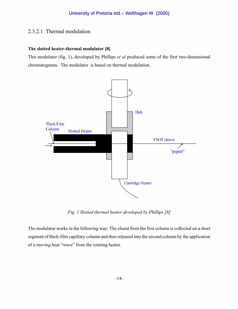
The slotted heater-thermal modulator [8]
This modulator (fig. 1), developed by Phillips et al produced some of the first two-dimensional
chromatograms. The modulator is based on thermal modulation.
Fig. 1 Slotted thermal heater developed by Phillips [8]
The modulator works in the following way: The eluent from the first column is collected on a short
segment of thick-film capillary column and then released into the second column by the application
of a moving heat “wave” from the rotating heater.
UUnniivveerrssiittyy ooff PPrreettoorriiaa eettdd –– WWeelltthhaaggeenn WW ((22000055))
-15-
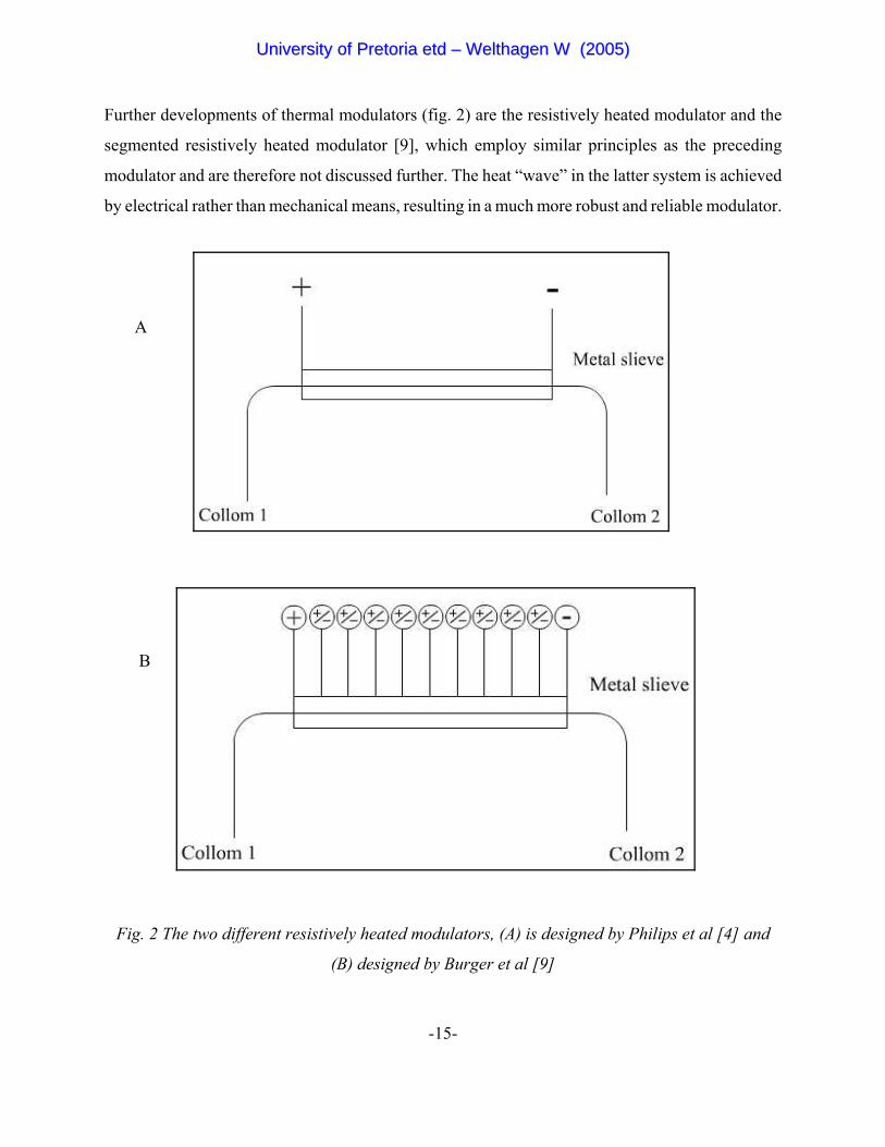
Further developments of thermal modulators (fig. 2) are the resistively heated modulator and the
segmented resistively heated modulator [9], which employ similar principles as the preceding
modulator and are therefore not discussed further. The heat “wave” in the latter system is achieved
by electrical rather than mechanical means, resulting in a much more robust and reliable modulator.
A
B
Fig. 2 The two different resistively heated modulators, (A) is designed by Philips et al [4] and
(B) designed by Burger et al [9]
UUnniivveerrssiittyy ooff PPrreettoorriiaa eettdd –– WWeelltthhaaggeenn WW ((22000055))
-16-
2.3.2.2 Cryofocussing modulation
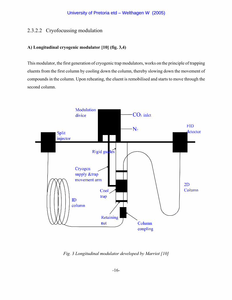
A) Longitudinal cryogenic modulator [10] (fig. 3,4)
This modulator, the first generation of cryogenic trap modulators, works on the principle of trapping
eluents from the first column by cooling down the column, thereby slowing down the movement of
compounds in the column. Upon reheating, the eluent is remobilised and starts to move through the
second column.
Fig. 3 Longitudinal modulator developed by Marriot [10]
UUnniivveerrssiittyy ooff PPrreettoorriiaa eettdd –– WWeelltthhaaggeenn WW ((22000055))
-17-
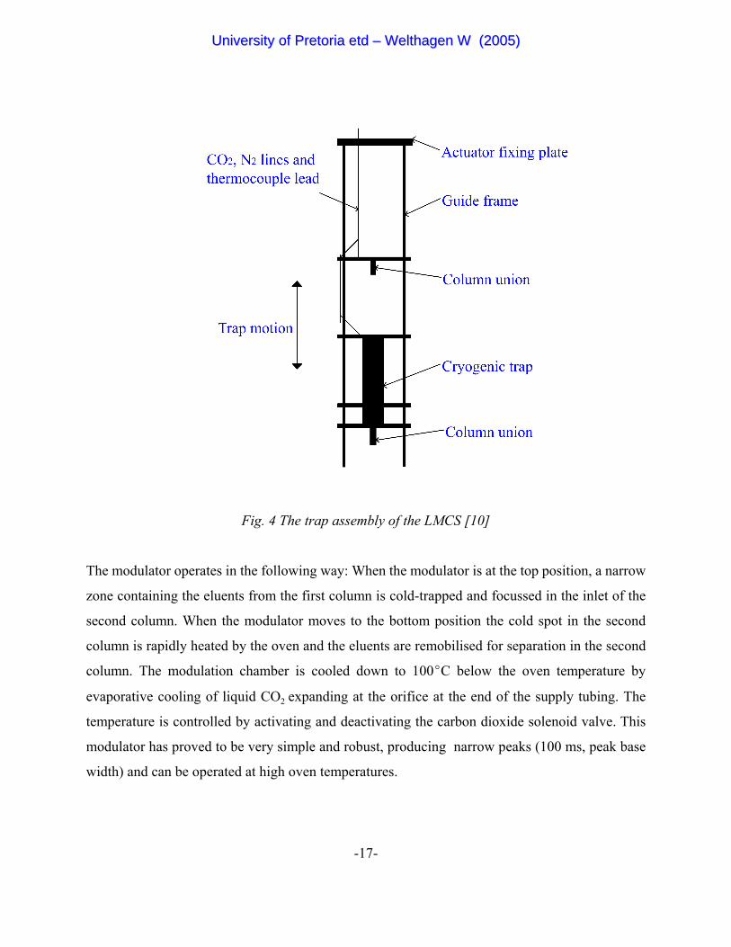
Fig. 4 The trap assembly of the LMCS [10]
The modulator operates in the following way: When the modulator is at the top position, a narrow
zone containing the eluents from the first column is cold-trapped and focussed in the inlet of the
second column. When the modulator moves to the bottom position the cold spot in the second
column is rapidly heated by the oven and the eluents are remobilised for separation in the second
column. The modulation chamber is cooled down to 100EC below the oven temperature by
evaporative cooling of liquid CO2 expanding at the orifice at the end of the supply tubing. The
temperature is controlled by activating and deactivating the carbon dioxide solenoid valve. This
modulator has proved to be very simple and robust, producing narrow peaks (100 ms, peak base
width) and can be operated at high oven temperatures.
UUnniivveerrssiittyy ooff PPrreettoorriiaa eettdd –– WWeelltthhaaggeenn WW ((22000055))
-18-
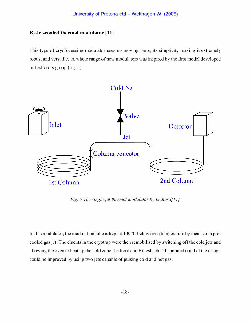
B) Jet-cooled thermal modulator [11]
This type of cryofocussing modulator uses no moving parts, its simplicity making it extremely
robust and versatile. A whole range of new modulators was inspired by the first model developed
in Ledford’s group (fig. 5).
Fig. 5 The single-jet thermal modulator by Ledford[11]
In this modulator, the modulation tube is kept at 100EC below oven temperature by means of a pre-
cooled gas jet. The eluents in the cryotrap were then remobilised by switching off the cold jets and
allowing the oven to heat up the cold zone. Ledford and Billesbach [11] pointed out that the design
could be improved by using two jets capable of pulsing cold and hot gas.
UUnniivveerrssiittyy ooff PPrreettoorriiaa eettdd –– WWeelltthhaaggeenn WW ((22000055))
-19-
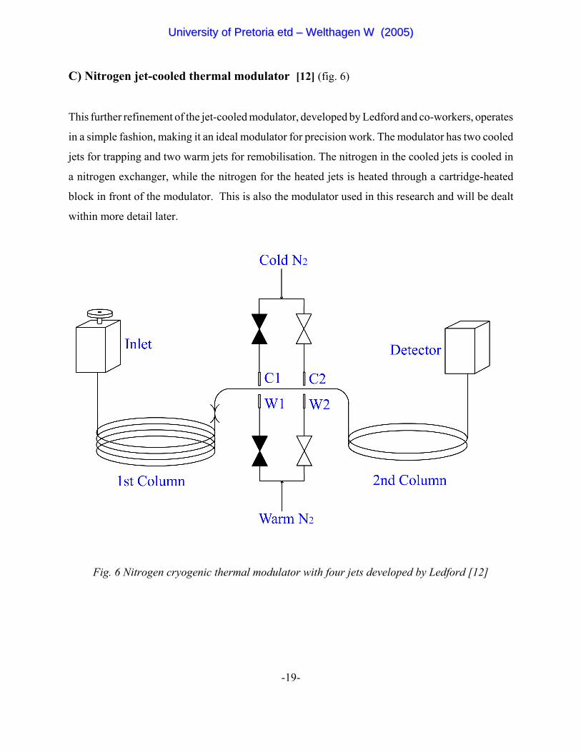
C) Nitrogen jet-cooled thermal modulator [12] (fig. 6)
This further refinement of the jet-cooled modulator, developed by Ledford and co-workers, operates
in a simple fashion, making it an ideal modulator for precision work. The modulator has two cooled
jets for trapping and two warm jets for remobilisation. The nitrogen in the cooled jets is cooled in
a nitrogen exchanger, while the nitrogen for the heated jets is heated through a cartridge-heated
block in front of the modulator. This is also the modulator used in this research and will be dealt
within more detail later.
Fig. 6 Nitrogen cryogenic thermal modulator with four jets developed by Ledford [12]
UUnniivveerrssiittyy ooff PPrreettoorriiaa eettdd –– WWeelltthhaaggeenn WW ((22000055))
-20-
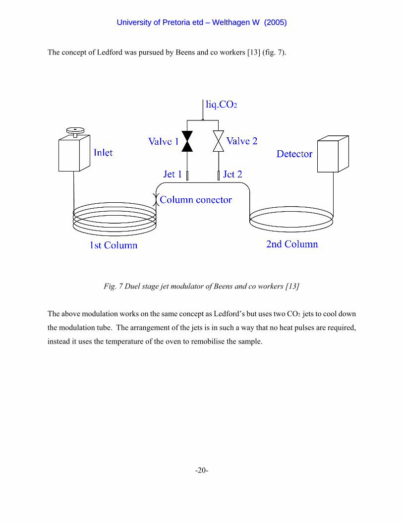
The concept of Ledford was pursued by Beens and co workers [13] (fig. 7).
Fig. 7 Duel stage jet modulator of Beens and co workers [13]
The above modulation works on the same concept as Ledford’s but uses two CO2 jets to cool down
the modulation tube. The arrangement of the jets is in such a way that no heat pulses are required,
instead it uses the temperature of the oven to remobilise the sample.
UUnniivveerrssiittyy ooff PPrreettoorriiaa eettdd –– WWeelltthhaaggeenn WW ((22000055))
-21-
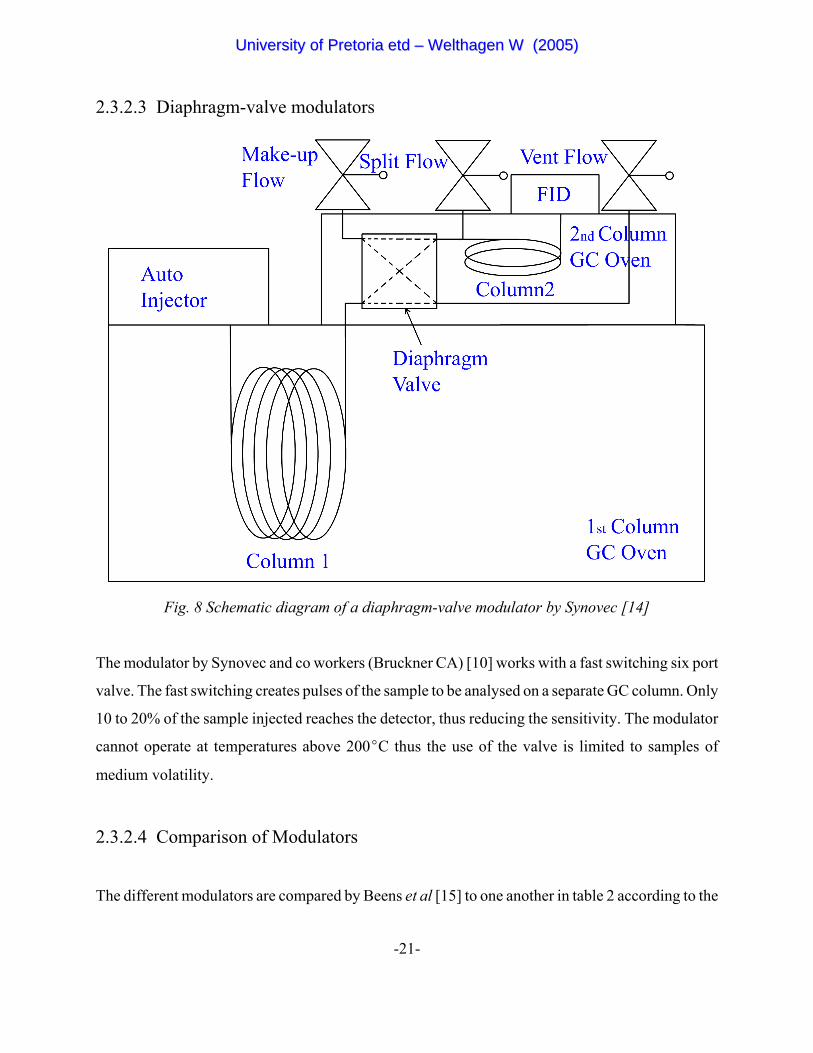
2.3.2.3 Diaphragm-valve modulators
Fig. 8 Schematic diagram of a diaphragm-valve modulator by Synovec [14]
The modulator by Synovec and co workers (Bruckner CA) [10] works with a fast switching six port
valve. The fast switching creates pulses of the sample to be analysed on a separate GC column. Only
10 to 20% of the sample injected reaches the detector, thus reducing the sensitivity. The modulator
cannot operate at temperatures above 200EC thus the use of the valve is limited to samples of
medium volatility.
2.3.2.4 Comparison of Modulators
The different modulators are compared by Beens et al [15] to one another in table 2 according to the
UUnniivveerrssiittyy ooff PPrreettoorriiaa eettdd –– WWeelltthhaaggeenn WW ((22000055))
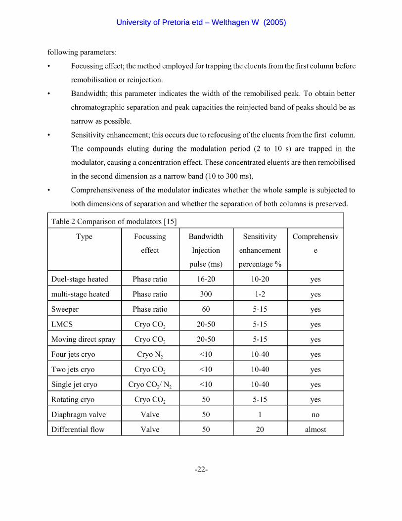
-22-
following parameters:
• Focussing effect; the method employed for trapping the eluents from the first column before
remobilisation or reinjection.
• Bandwidth; this parameter indicates the width of the remobilised peak. To obtain better
chromatographic separation and peak capacities the reinjected band of peaks should be as
narrow as possible.
• Sensitivity enhancement; this occurs due to refocusing of the eluents from the first column.
The compounds eluting during the modulation period (2 to 10 s) are trapped in the
modulator, causing a concentration effect. These concentrated eluents are then remobilised
in the second dimension as a narrow band (10 to 300 ms).
• Comprehensiveness of the modulator indicates whether the whole sample is subjected to
both dimensions of separation and whether the separation of both columns is preserved.
Table 2 Comparison of modulators [15]
Type Focussing
effect
Bandwidth
Injection
pulse (ms)
Sensitivity
enhancement
percentage %
Comprehensiv
e
Duel-stage heated Phase ratio 16-20 10-20 yes
multi-stage heated Phase ratio 300 1-2 yes
Sweeper Phase ratio 60 5-15 yes
LMCS Cryo CO2 20-50 5-15 yes
Moving direct spray Cryo CO2 20-50 5-15 yes
Four jets cryo Cryo N2 <10 10-40 yes
Two jets cryo Cryo CO2 <10 10-40 yes
Single jet cryo Cryo CO2/ N2 <10 10-40 yes
Rotating cryo Cryo CO2 50 5-15 yes
Diaphragm valve Valve 50 1 no
Differential flow Valve 50 20 almost
UUnniivveerrssiittyy ooff PPrreettoorriiaa eettdd –– WWeelltthhaaggeenn WW ((22000055))
-23-
The cryogenic jet modulators have the narrowest injection pulses and the biggest peak enhancement
of all the modulators available. The cryogenic jet modulators thus outperform the other designs and
is a popular choice where the cost of gas and liquid nitrogen can be ignored.
2.3.3 Detectors in GC x GC
For GC x GC peak detection, a fast detector is needed. The peak widths on the second dimension
are in the order of 20 ms [16] at the head of the modulator and 100 ms to 200 ms at elution. Thus,
to have a representative number of detection points per peak ( for instance, at least ten points per
peak) the sampling rate of the detector should be at least 100 Hz. The most common detector used
in almost all GC x GC separations is the FID (flame ionisation detector) due to its speed (easily
allowing sampling at 200 Hz). Any other GC detector which has a similar sample rate could also be
used.
While mass spectrometry, as in all other GC applications, could enhance the identification of peaks,
most mass spectrometers lack a satisfactory sampling rate, with the exception of the TOFMS (time-
of-flight mas spectrometer) which can have a sampling rate of up to 500 Hz [17].
2.3.4 Interpretation of GC x GC separation
In order to interpret a GC x GC chromatogram, it is essential to understand the separation of
compounds in different dimensions. The assumption of random distributions in one-dimensional
chromatography [18,19] provided valuable information in the understanding of peak distributions
in a chromatographic axis. However, peak distribution is not truly random: All the components in
the mixture have definite structures and must be directed to definite locations in retention space
based on these structures [20].
UUnniivveerrssiittyy ooff PPrreettoorriiaa eettdd –– WWeelltthhaaggeenn WW ((22000055))
-24-
Giddings [21] showed theoretically that the key property of a separation method, which determines
whether or not it can show the inherent structure of a mixture being separated, is the method’s
dimensionality that should match the dimensionality of the mixture. The dimensionality of a mixture
is the number of independent variables in which the members of the mixture can be separated. When
a mixture is then separated according to these independent variables (by a system of matching
dimensionality), each type of compound will separate to a unique location on the separation
plane(chromatogram). However, as indicated above, the compounds are composed of molecules
with discrete structures that are related, the compounds must thus distribute over the dimensional
separation space (chromatogram) to discrete locations which are also related to each other [21].
To explain the Giddings theory, separation in GC x GC is used as an example: If a mixture is
separated into one dimension, such as the boiling point fractions in petroleum samples, the alkanes
and the aromatics with similar boiling points will overlap and thus insignificant ordering of
compounds occurs. If the variable “boiling point” is changed to “polarity” the same overlap does
not occur but a new overlap is created by different “boiling point” fractions, thus the separation or
ordering is still insignificant. The mixture is simply not sufficiently well ordered in any one
dimension, it requires at least two matching independent variables to uniquely separate the
compounds of the mixture.
GC x GC chromatograms (volatility x polarity separation, method dimensionality of two) of
petroleum fractions are highly ordered, indicating that these samples have a dimensionality of two
(can be classified by either volatility or polarity) , for most of their components [19]. Ordered
chromatograms have the potential advantage of being more interpretable than disordered ones. The
pattern of peak placement is highly informative by itself and may make it possible to identify most
or all of the components of a given mixture.
UUnniivveerrssiittyy ooff PPrreettoorriiaa eettdd –– WWeelltthhaaggeenn WW ((22000055))
-25-
2.3.5 GC x GC vs GC - GC
GC x GC is a term used to describe a comprehensive two-dimensional technique where the entire
sample separated by the first dimension column is subjected to separation by the second column. GC
- GC, in contrast, is not a comprehensive technique, as it works on the basis of taking specific
sections of the elution profile from the first dimension and subjecting those discrete sections to
further separation on a second column.
Chromatographic resolution of complex samples can be improved by increased peak capacity, for
example by increasing the length of the column. Resolution, however, only increases by the square
root of column length and is finally limited by pressure drop requirements of the carrier gas. It could
thus be a very expensive exercise to increase peak capacity on a single column when mixtures are
truly complex. Two-dimensional chromatography offers a new way of increasing peak capacity.
Many variations of two-dimensional chromatography exist. The “heart cut” method where a segment
of the elution of the first column is injected into a second column of different stationary phase,
provides good separation of compounds but is very time consuming if repetitive injections have to
be made in order to analyse all first dimension sections also on the second dimension. This could
take weeks for a complex sample.
The peak capacity of a GC - GC system (single heart-cut) is only the peak capacity of the first
column plus the peak capacity of the second dimension column. In the case of GC x GC the total
time of analysis is decreased and provides a full overview of the sample in two dimensions with the
overall peak capacity equal to the first dimension’s peak capacity multiplied by the peak capacity
of the second dimension. Due to the high speed requirement of the second-dimension of GC x GC
it does not have the same peak capacity as the second dimension in GC - GC. The overall peak
capacity generated per time scale is, however, much higher. The overall peak capacity of GC x GC
can be further improved by lengthening the columns or slowing down the first-dimension
temperature program, but this unfortunately will result in a much longer total analysis time.
UUnniivveerrssiittyy ooff PPrreettoorriiaa eettdd –– WWeelltthhaaggeenn WW ((22000055))
-26-
Chapter 3
Background: Part 2
GC x GC optimisation
Table of contents
3.1 Introduction
3.2 One dimensional GC considerations
3.2.1 Column stationary phase
3.2.2 Column dimensions
3.2.3 Linear flow rate
3.2.4 Temperature considerations
3.2.5 Fast isothermal GC
3.2.6 Injection techniques
3.3 Combining the two columns
3.4 Conclusions
UUnniivveerrssiittyy ooff PPrreettoorriiaa eettdd –– WWeelltthhaaggeenn WW ((22000055))
-27-
Chapter 3
Background: Part 2
Optimisation of a GC x GC system
3.1 Introduction
The analytical requirements will dictate the type of optimisation required by a particular
chromatographic separation. Some optimisation goals are: resolution, sample capacity and speed
of analysis. When all the components of a very complex mixture need to be determined,
chromatographic separation is optimised for maximum resolution in order to measure the maximum
number of peaks. Another type of optimisation has as goal the fastest analysis time. This type of
chromatographic separation is often required in process control where fast response times are
essential. Faster analysis times often results in decreased resolution.
GC x GC provides us with a means to minimise the speed/resolution trade-off. Because of its greatly
increased peak capacity, it can be used for quality control processes where many compounds need
to be resolved, in a time-efficient manner.
The GC x GC system consists of two different columns, the first column is run under normal GC
conditions and the second under fast GC conditions. Therefore, optimising the two columns involve
two separate sets of conditions. The optimisation, however, is complicated by the fact that the two
columns are serially connected to each other. This results in changes to the one set of conditions
having an effect on the other.
Each column can be studied individually before considering the additional constraints of a coupled
system. In this chapter, the parameters of each chromatographic system (normal GC and Fast GC)
are discussed, followed by the new parameters required by joining the two systems.
UUnniivveerrssiittyy ooff PPrreettoorriiaa eettdd –– WWeelltthhaaggeenn WW ((22000055))
-28-
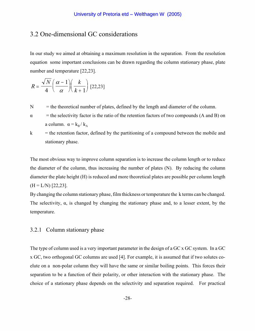
3.2 One-dimensional GC considerations
In our study we aimed at obtaining a maximum resolution in the separation. From the resolution
equation some important conclusions can be drawn regarding the column stationary phase, plate
number and temperature [22,23].
[22,23]RN k
k=
−⎛⎝⎜
⎞⎠⎟ +⎛⎝⎜
⎞⎠⎟4
11
αα
N = the theoretical number of plates, defined by the length and diameter of the column.
α = the selectivity factor is the ratio of the retention factors of two compounds (A and B) on
a column. α = kB / kA
k = the retention factor, defined by the partitioning of a compound between the mobile and
stationary phase.
The most obvious way to improve column separation is to increase the column length or to reduce
the diameter of the column, thus increasing the number of plates (N). By reducing the column
diameter the plate height (H) is reduced and more theoretical plates are possible per column length
(H = L/N) [22,23].
By changing the column stationary phase, film thickness or temperature the k terms can be changed.
The selectivity, α, is changed by changing the stationary phase and, to a lesser extent, by the
temperature.
3.2.1 Column stationary phase
The type of column used is a very important parameter in the design of a GC x GC system. In a GC
x GC, two orthogonal GC columns are used [4]. For example, it is assumed that if two solutes co-
elute on a non-polar column they will have the same or similar boiling points. This forces their
separation to be a function of their polarity, or other interaction with the stationary phase. The
choice of a stationary phase depends on the selectivity and separation required. For practical
UUnniivveerrssiittyy ooff PPrreettoorriiaa eettdd –– WWeelltthhaaggeenn WW ((22000055))
-29-
reasons the first-dimension stationary phase is generally chosen to perform a volatility separation.
The most common of these stationary phases is listed in table 3 [ 24].
Table 3 Different non-polar stationary phases [24]
100% dimethyl
polysiloxane
5% diphenyl - 95% dimethyl
polysiloxane
6% cyanopropylphenyl
94% dimethyl polysiloxane
non-polar non-polar slightly polar
The selection of a second-dimension column is more critical. Separation on the second column is
dictated by the selective interaction of the sample with the stationary phase. Therefore, the choice
of second dimension column will be based on the sample and what selectivity is required [22,23].
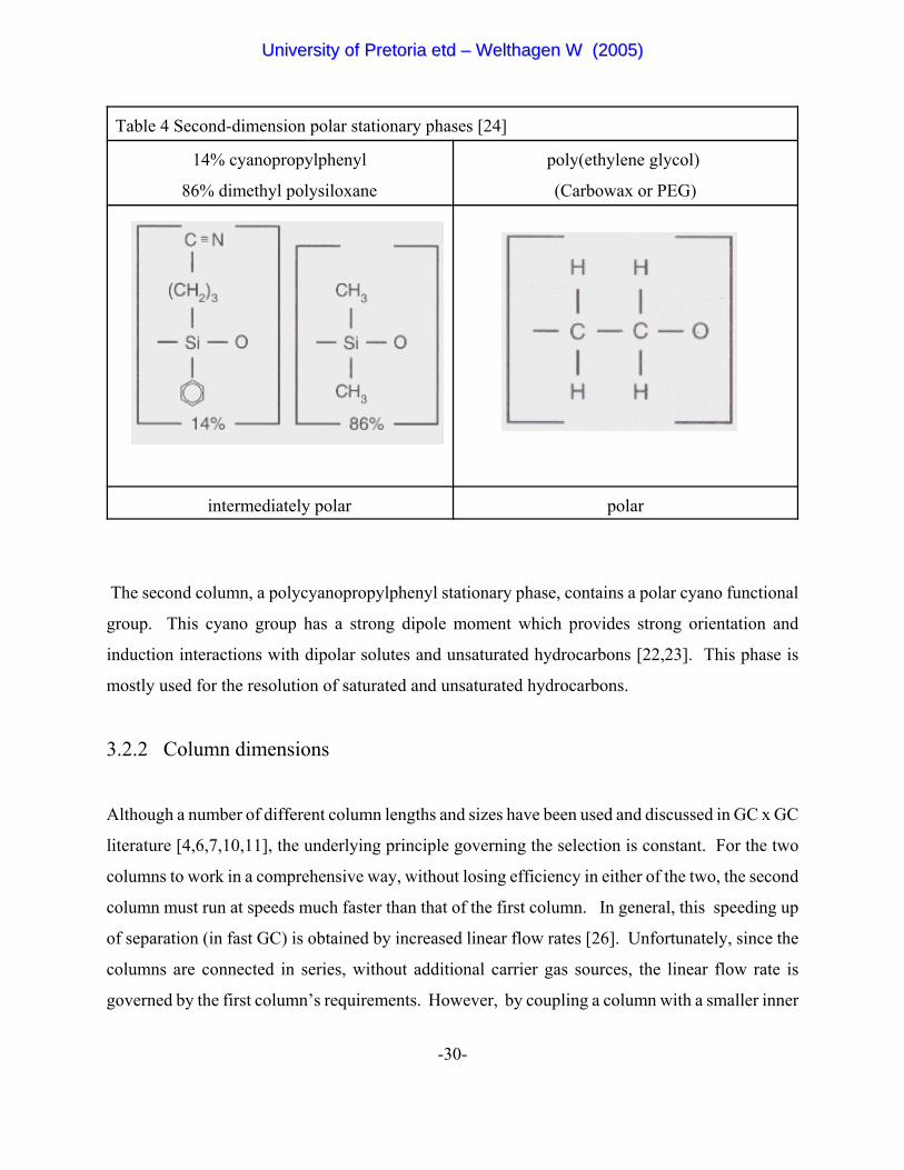
The most common of these stationary phases is listed in table 4 [ 24]. For example, in this study, two
second dimension columns were used. The first column had a poly-ethylene glycol stationary
phase, HO(CH2CH2O)nCH2CH2OH. This stationary phase contains hydroxyl groups that can
undergo hydrogen bonding with oxygenated compounds, making it an ideal column for the
resolution of oxygenated compounds (particularly alcohols) and other polar solutes [25].
UUnniivveerrssiittyy ooff PPrreettoorriiaa eettdd –– WWeelltthhaaggeenn WW ((22000055))
-30-
Table 4 Second-dimension polar stationary phases [24]
14% cyanopropylphenyl
86% dimethyl polysiloxane
poly(ethylene glycol)
(Carbowax or PEG)
intermediately polar polar
The second column, a polycyanopropylphenyl stationary phase, contains a polar cyano functional
group. This cyano group has a strong dipole moment which provides strong orientation and
induction interactions with dipolar solutes and unsaturated hydrocarbons [22,23]. This phase is
mostly used for the resolution of saturated and unsaturated hydrocarbons.
3.2.2 Column dimensions
Although a number of different column lengths and sizes have been used and discussed in GC x GC
literature [4,6,7,10,11], the underlying principle governing the selection is constant. For the two
columns to work in a comprehensive way, without losing efficiency in either of the two, the second
column must run at speeds much faster than that of the first column. In general, this speeding up
of separation (in fast GC) is obtained by increased linear flow rates [26]. Unfortunately, since the
columns are connected in series, without additional carrier gas sources, the linear flow rate is
governed by the first column’s requirements. However, by coupling a column with a smaller inner
UUnniivveerrssiittyy ooff PPrreettoorriiaa eettdd –– WWeelltthhaaggeenn WW ((22000055))
-31-
diameter to the first column a faster linear flow rate of the second column and thus faster separation
speed is advised. The most common choice of columns is a 250 Fm inner diameter column coupled
to a 100 Fm column.
3.2.3 Linear flow rate
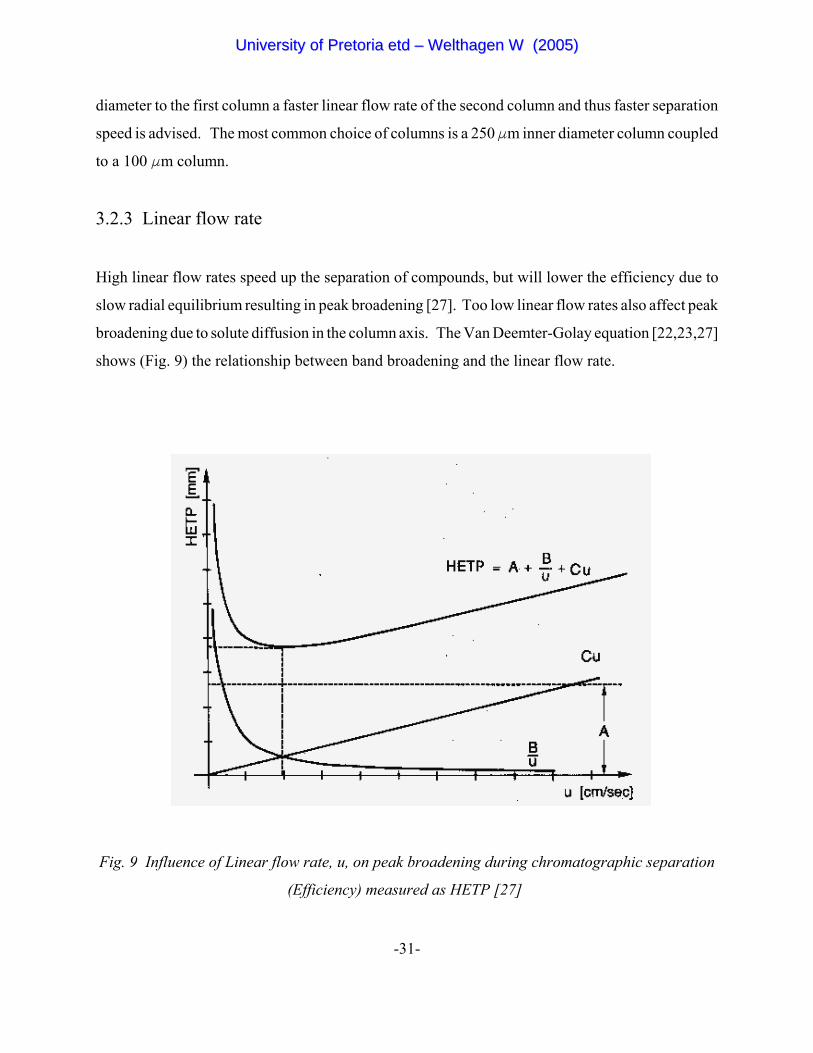
High linear flow rates speed up the separation of compounds, but will lower the efficiency due to
slow radial equilibrium resulting in peak broadening [27]. Too low linear flow rates also affect peak
broadening due to solute diffusion in the column axis. The Van Deemter-Golay equation [22,23,27]
shows (Fig. 9) the relationship between band broadening and the linear flow rate.
Fig. 9 Influence of Linear flow rate, u, on peak broadening during chromatographic separation
(Efficiency) measured as HETP [27]
UUnniivveerrssiittyy ooff PPrreettoorriiaa eettdd –– WWeelltthhaaggeenn WW ((22000055))
-32-
In the Van Deemter-Golay equation, band broadening is expressed as HETP, the sum of the
following terms [22,23,27]:
Cu = The dominant cause of band broadening at high flow rates is the resistance to mass transfer,
preventing the existence of an instantaneous equilibrium between solute, stationary phase
and mobile phase. The term increases in proportion to linear flow rate, u.
A = Different pathways (packed columns only) have different lengths in the same column. This
packed column parameter is flow independent.
B/u = Longitudinal diffusion (diffusion of solute in the axial direction), increases with the time
spent in the column and is therefore inversely proportional to the linear flow rate.
The van Deemter-Golay equation is widely accepted by chromatographers around the world and
defines the strategy for optimising flow rates.
3.2.4 Temperature considerations
Next to selecting the stationary phase, temperature is the most important parameter in a GC system
to be optimised [22,23,27]. Temperature has an influence on retention of analytes (k) and to a lesser
extent selectivity between analytes (α). Temperature thus needs to be optimised for practical
considerations such as analysis speed, sample type and aim of analysis [22,23,27].
In the scope of a GC x GC system some more considerations need to be addressed. High separation
efficiency is required from the first column which needs to be preserved in the rest of the system.
Since the modulator combines already separated segments during the trapping stage, which is the
length of time required by the second separation, the peaks eluting from the first column should be
as wide as possible, without losing first-dimension (1D) resolution. This can be achieved by slowing
down the temperature ramp used in the first dimension.
The second consideration in GC x GC temperatures is that the modulation period is often shorter
than the separation time needed in the second-dimension (2D). This problem is addressed by
UUnniivveerrssiittyy ooff PPrreettoorriiaa eettdd –– WWeelltthhaaggeenn WW ((22000055))
-33-
0
0.2
0.4
0.6
0.8
1
0 5 10 15 20Retention factor, k
k/(k
+1)
increasing the temperature in the second dimension. The increase in temperature speeds up the
elution, but with a trade-off to resolution between compounds in the early part of the chromatogram.
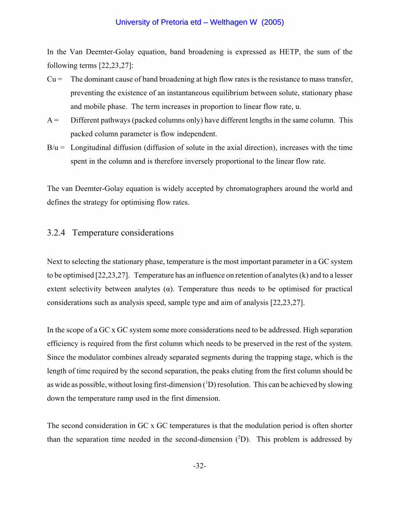
This well-known dilemma in chromatography is referred to as the general elution problem [23]. The
graph of k/(k+1) against k in figure 10 explains, in terms of the resolution equation in paragraph 3.2,
how the resolution drastically drops when k approaches zero. (If k/(k+1) .0, R . 0).
Fig. 10 The graph of k/(k+1) against k [23]
Ideally a fast temperature-programmed GC could be used in the second dimension, but up to date
there is no such development.
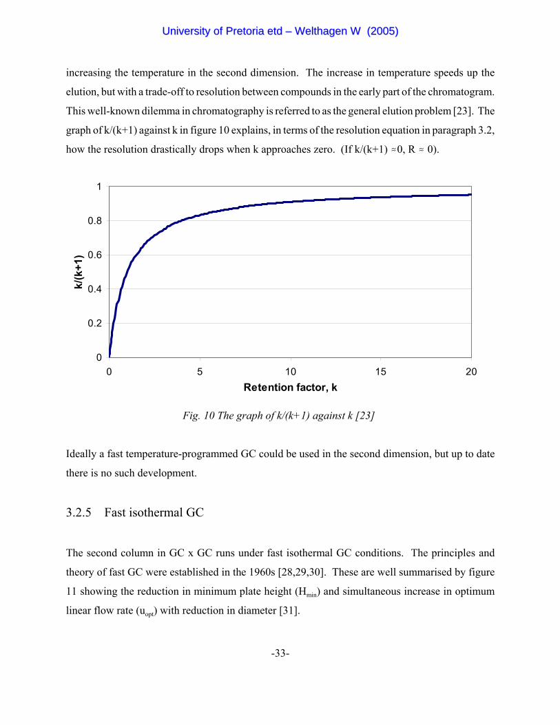
3.2.5 Fast isothermal GC
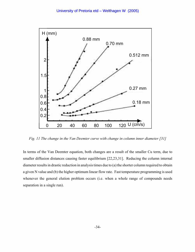
The second column in GC x GC runs under fast isothermal GC conditions. The principles and
theory of fast GC were established in the 1960s [28,29,30]. These are well summarised by figure
11 showing the reduction in minimum plate height (Hmin) and simultaneous increase in optimum
linear flow rate (uopt) with reduction in diameter [31].
UUnniivveerrssiittyy ooff PPrreettoorriiaa eettdd –– WWeelltthhaaggeenn WW ((22000055))
-34-
0 20 40 60 80 100 120 U (cm/s)
0.20.40.60.8
1
1.5
2
H (mm)
0.18 mm
0.27 mm
0.512 mm
0.70 mm0.88 mm
0 20 40 60 80 100 120 U (cm/s)
0.20.40.60.8
1
1.5
2
H (mm)
0.18 mm
0.27 mm
0.512 mm
0.70 mm0.88 mm
Fig. 11 The change in the Van Deemter curve with change in column inner diameter [31]
In terms of the Van Deemter equation, both changes are a result of the smaller Cu term, due to
smaller diffusion distances causing faster equilibrium [22,23,31]. Reducing the column internal
diameter results in drastic reduction in analysis times due to (a) the shorter column required to obtain
a given N value and (b) the higher optimum linear flow rate. Fast temperature programming is used
whenever the general elution problem occurs (i.e. when a whole range of compounds needs
separation in a single run).
UUnniivveerrssiittyy ooff PPrreettoorriiaa eettdd –– WWeelltthhaaggeenn WW ((22000055))
-35-
3.2.6 Injection techniques
The injection bandwidth is probably just as important as optimising temperatures or flow rates. The
resolution, and thus efficiency, of peaks is greatly dependant on the peak widths. Thus it is very
important that peak broadening is only due to the van Deemter parameters discussed in section
(3.2.3) and not due to a bad injection.
In a temperature-programmed GC a bad injection is masked by thermal focussing on the cool
column at the start of the run (the compounds only starts moving after a specific temperature is
reached). In an isothermal GC there is no such a thing as thermal focussing at low initial
temperatures and all compounds start moving at the same time. Therefore much work was done on
perfecting injection techniques for fast GC [32].
3.3 Combining the two columns
When combining the two columns new aspects in the optimisation process need to be addressed.
The two columns are connected in serries, implying that a change on one column would have an
effect on the other. These kinds of changes include column lengths (3.2.2), carrier gas flow (3.2.3),
pressures (3.2.5.1) and temperature programming (3.2.4) [33].
When combining two columns the interface responsible for linking the two, called the modulator
(2.3.3), also needs to be optimised. The modulator in this study, the nitrogen jet-cooled modulator,
needs to be optimised for modulator temperature, gas flows of heating and cooling gases, duration
of heating and cooling pulses and duration of modulation period.
UUnniivveerrssiittyy ooff PPrreettoorriiaa eettdd –– WWeelltthhaaggeenn WW ((22000055))

-36-
3.4 Conclusions
Optimising a single column by now is trivial and is done routinely around the world. By adding a
second dimension, we increase the complexity of the optimisation and new strategies need to be
developed.
UUnniivveerrssiittyy ooff PPrreettoorriiaa eettdd –– WWeelltthhaaggeenn WW ((22000055))
-37-
Chapter 4
Background: Part 3
The analysis of petrochemical samples
Table of Contents
4.1 Introduction
4.2 Gas Chromatography (GC)
4.2.1 Simulated distillation (SimDist)
4.2.2 PIONA analysis
4.3 GC x Selective Detector
4.4 GC x GC
4.5 GC x GC x Selective Detector
4.6 Other applications of GC x GC
2.6.1 Fast screening
2.6.2 Environmental samples
4.7 Conclusions
UUnniivveerrssiittyy ooff PPrreettoorriiaa eettdd –– WWeelltthhaaggeenn WW ((22000055))
-38-
Chapter 4
Background: Part 3
The analysis of petrochemical samples
4.1 Introduction
Petrochemical samples are extremely complex in nature, not only do they contain many thousands
of compounds but they also show characteristic bulk behaviour, dependent on their quantitative and
qualitative sample composition. The analysis of these samples thus not only requires the
identification of all the individual components but also to the charting of compositional patterns
associated with different bulk characteristics. It is mostly these characteristic properties of the
samples that are of economic interest to manufacturers. The traditional methods of characterising
petrochemical samples involved direct bulk measurement of viscosity, density, pour point, flash
point, etc. These methods provide a fast, simple answer to many of the bulk characteristics, but
require many analyses and are not always informative enough. The intensive studies of
petrochemical analysis lead to the development of many analytical techniques, including
chromatography. Some of these developments are discussed in the following sections.
4.2 Gas Chromatography (GC)
The separation potential of gas chromatography was already predicted by Martin [33] in the 1950's.
Squalane [34] coated metal capillaries were first used for the characterisation of hydrocarbon
mixtures [5]. These columns were used until the early 1980s, but although they produced good
“repeatable” results [35], they were limited to temperatures below 90EC. Glass capillaries were first
reported by Grob et al in 1969 [36,37], but due to their fragility they were only used by a small
UUnniivveerrssiittyy ooff PPrreettoorriiaa eettdd –– WWeelltthhaaggeenn WW ((22000055))
-39-
group of scientist. After the development of the fused-silica column by Dandeneau and Zerenner
in 1978 [38], the use of capillary columns became widely accepted. During the same time period,
advances such as cross-linking polymeric films in-situ and chemically bonding stationary phases to
the silica surface increased the temperature limits of the columns [5].
The detailed-hydrocarbon analyser (DHA), a 100m long column designed to separate straight-run
hydrocarbon fractions is, to this date, the ultimate use of separation power in linear capillary
chromatography within the petrochemical industry [5]. This approach virtually identified all
hydrocarbons in petrochemical fractions up to C9, but samples that contained substantial quantities
of olefins could not be separated into their individual components [5].
4.2.1 Simulated distillation (SimDist)
Distillation is one of the most important techniques in the petrochemical industry. Distillation data
are used for the characterisation of feedstock, products and for process control. Boiling-range
distributions were among the first tests documented by the American Society for Testing and
Materials (ASTM) in 1921, and this distillation test is still used today [5].
The similarity between a non-polar column separation and distillation data made chromatography
an attractive, faster alternative for distillation testing. By running standards, usually a series of n-
alkanes, the boiling points of which are accurately known, the retention-time axis can be converted
into a boiling-point scale. This approach first achieved formal status in 1973 as ASTM D2887 [5].
The method covered diesel, fuel oil, and light lubricants, with boiling points up to 540EC (n-C44).
The invention of capillary columns further extended the temperature range of the hydrocarbons
analysed. The first reported simulated distillation use of capillary columns by Luke and Ray in 1985
[39] separated hydrocarbons up to a boiling point of 650EC (n-C70), but it was fast followed by
Trestianu et al.[40] with their High-Temp Simdist method capable of eluting compounds up to C120
at 430EC and up to C140 in the final isothermal hold. These new developments eclipsed the use of
normal distillation as, even under reduced vacuum conditions, alkanes above C60 cannot be distilled
[5].
UUnniivveerrssiittyy ooff PPrreettoorriiaa eettdd –– WWeelltthhaaggeenn WW ((22000055))
-40-
4.2.2 PIONA analysis
The complexity of petrochemical products and processes lead to the development of the selectively
coupled column systems, which are still in use today, the PIONA. The first of these coupled systems
was a GC-GC-GC system, the PNA[41], which could separate oil fractions up to 200EC into distinct
chemical classes, the Paraffins (P), the Naphthenes or cyclic paraffins (N) and the Aromatics (A).
The system has been improved over the years and the number of separation steps increased, resulting
in a PIONA analyser [42] with GC-GC-GC-GC-GC couplings. It could now also separate and group
the Iso-alkanes (I) and the alkenes or Olefins (O). This technique is known as a coupled column
technique, but the entire sample is not submitted to every individual separation step. The only
similarity between this technique and modern comprehensive techniques is that the entire sample
eventually reaches the detector [5].
4.3 GC x Selective Detector
In the petroleum industry, the separation of compounds is sometimes insufficient, therefore a
number of selective detectors have been developed for their analysis and characterisation. The most
common of these detectors is [5]:
• the Flame-Photometric Detector (FPD) designed for sulphur detection
• the Nitrogen-Phosphorus Detector (NPD)
• the Atomic Emission Detector (AED) for various elements
• the Chemiluminescence Detector for sulphur detection
• the oxygen Flame-Ionisation Detector (OFID) adapted to detect oxygenates
• the Mass Spectrometer (MS), which is the most versatile detector.
The petroleum industry pioneered the development of the mass spectrometer. The first commercial
MS was sold to a petrochemical industry (Atlantic Refining Company in 1946 for the analysis of
hydrocarbon fractions in the gasoline boiling range) [43]. The first mass spectrometers worked on
a direct injection basis and were limited, as compared to GC, in that they could not detect isomers
UUnniivveerrssiittyy ooff PPrreettoorriiaa eettdd –– WWeelltthhaaggeenn WW ((22000055))
-41-
[5]. The coupling of GC to MS became a logical next step in the development of GC- detectors to
improve complex mixture detection [44].
4.4 GC x GC
As discussed before, the potential of GC x GC to increase peak capacity beyond that of conventional
capillary GC by about 50 times, already provides an attractive alternative to researchers in the
petrochemical industry. Although the peak capacity is a big factor, the biggest attraction lies within
the method’s capability of arranging compounds in chemical classes, greatly simplifying
identification and target analysis [45,46]. The sweeper modulated system is somewhat limited in
application, as it cannot focus highly volatile compounds, while non-volatile “heavy” compounds
require temperatures exceeding current column and modulator capabilities [5]. The optimum
performance range of the sweeper, C10-C16 hydrocarbons, is, however, of immediate practical
interest because the sophisticated methods (PIONA and DHA) developed for gasolines and naphthas
are unsatisfactory in this range [5]. The recent introduction of the jet-cooled modulator [6,7] and
independent temperature control of the first and second oven, are increasing the volatility range of
compounds that can be analysed by GC x GC [47].
4.5 GC x GC coupled to a Selective Detector
Selective detectors will surely increase the scope and dimensions of GC x GC, therefore it is just a
matter of time before detectors, such as the Atomic Emision-Detection (AED), are coupled to the
system. The most important criterium for GC x GC detectors, as described in chapter 3, is their
response speed. With this in mind, the only MS which can be coupled to GC x GC is the TOFMS.
The initial steps of combining the two has already been taken [48], the GC x GC - TOFMS has been
used for the quantification of aromatic compounds and sulphur containing compounds in petroleum
samples.
UUnniivveerrssiittyy ooff PPrreettoorriiaa eettdd –– WWeelltthhaaggeenn WW ((22000055))
-42-
4.6 Other applications of GC x GC
Although the GC x GC is a good separation tool to separate complex mixtures of a hundred or more
components, it is even more useful in the separation of less complex mixtures, with a dimensionality
of two or three, due to its ordering capabilities. Common further applications are discussed below.
4.6.1 Fast screening
GC x GC has the ability to give a quick overview of a mixture, thus providing fast information to
identify or classify a mixture. The fingerprinting technique used in classifying and identifying
complex mixtures, for example quality control of essential oils, is demonstrated in the research done
in parallel by co-workers from our laboratory [49]. The second dimension can also be tuned to
unravel overlapping peaks for the analysis of trace components [50].
4.6.2 Environmental samples
Most environmental analyses have focussed on individual target substances and not the overall
mixture. This provides a limited understanding of the true situation. Gaines et al. used GC x GC
to determine trace oxygenates and aromatics in water samples [50]. Furthermore, this research group
developed a method for the quantitative determination of benzene, toluene, ethyl benzene and xylene
(BTEX) and total aromatic content of gasoline based on GC x GC [50]. They also used GC x GC
as an excellent tool to identify oil-spill sources of slightly weathered marine diesel fuel from surface
water [51].
UUnniivveerrssiittyy ooff PPrreettoorriiaa eettdd –– WWeelltthhaaggeenn WW ((22000055))

-43-
4.7 Conclusions
The technique of GC x GC is still relatively new, it was only a decade ago that Phillips [4]
introduced it to the world, but since its introduction it has taken the world by storm. The
capabilities of the technique are simply astounding. Its ability to unravel very complex mixtures into
structured chromatograms, or to reveal hidden trace peaks in complex matrices, has so far captured
the imagination of researchers. These remarkable capabilities remain untapped and will only be
unlocked with proper optimisation.
UUnniivveerrssiittyy ooff PPrreettoorriiaa eettdd –– WWeelltthhaaggeenn WW ((22000055))
-44-
Chapter 5
Optimisation of GC x GC parameters
Table of Contents
5.1 Introduction
5.2 General experimental setup
5.2.1 Instrumentation
5.2.2 Computer software5.2.2.1 Operating software
5.2.2.2 Data acquisition software
5.2.2.3 Data analysis and visualisation
5.2.3 Samples used
5.3 Optimising the column parameters
5.3.1 Linear flow rates
5.3.2 Optimisation of the flow rates for optimum resolution
5.3.3 Choice of second dimension stationary phase
5.3.4 Temperature difference between columns
5.4 Modulator optimisation
UUnniivveerrssiittyy ooff PPrreettoorriiaa eettdd –– WWeelltthhaaggeenn WW ((22000055))
-45-
Chapter 5
Optimisation of GC x GC parameters
5.1 Introduction
As discussed in Chapter 3, the optimisation of any system is the most important part before the start
of analysis. The fundamentals of optimising a two-dimensional gas chromatography system are
exactly the same as in normal one-dimensional gas chromatography. The difficulty in optimising
a two-dimensional system is that, instead of separately optimising only the parameters involved in
one gas chromatographic system, two integrated gas chromatographic systems have to be optimised
together.
For overall optimisation of a gas chromatographic system, it is necessary to follow a chronological
path in order to keep track of changes and eventually optimise all the different parameters.
Guidelines to optimise one-dimensional gas chromatography already exist, and it was also used as
a guideline to optimise the two-dimensional system. In this dissertation the optimisation strategy
included the:
• Linear flow rate in both columns
• Stationary phase selection of the second-dimension
• Temperature programming of the first- and second-dimension columns
• Optimisation of the modulator
• Atmospheric conditions influencing the modulator operation
This optimisation strategy represents a logical and sequential guide to optimise the different
parameters involved in GC x GC. The coupling of two chromatographic columns gives rise to some
more parameters to be optimised. These include the operation of the coupling interface (the
modulator) to trap and inject first-dimension eluents into the second-dimension and to achieve this
with minimal “wrap around” of second-dimension peaks. A wrap around occurs when the
UUnniivveerrssiittyy ooff PPrreettoorriiaa eettdd –– WWeelltthhaaggeenn WW ((22000055))
-46-
modulator injects the next elution portion of the first-dimension column before the second-
dimension separation of the previous portion is completed and overlap occurs between peaks of
successive second-dimension chromatograms.
The following sections are divided into the general experimental setup in which the optimisation was
done and a discussion of the different procedures to optimise the two-dimensional system.
5.2 General experimental setup
5.2.1 Instrumentation
The instrumental requirements for GC x GC are very similar to that of normal GC; in general a GC
oven is modified to include a modulator (or coupling interface) between the two chromatographic
columns. In addition to the modulator a second-dimension oven can be inserted into the main GC
oven to have independent temperature control of the second dimension. The rest of the instrument
is fundamentally the same, with an injector and a detector.
In our experiments an Agilent 6890A GC oven (Agilent Technologies,Wilmington, USA) was used,
fitted with an Agilent split/split less injector and a fast flame ionisation detector (FID). Hydrogen
was chosen as carrier gas, because of its good separation properties. Hydrogen is ideal for fast gas
chromatographic separations and where maximum separation is required in a fixed time. The
injector was set to 250EC with split mode, under constant pressure conditions. The FID operated
at 300EC with an airflow of 400 ml/min, hydrogen flow of 50 ml/min and nitrogen makeup of 50
ml/min. The signal obtained from the FID was recorded at 200 Hz.
The GC x GC modifications on this instrument were the following: A dual stage nitrogen cooled
modulator (Zoex corp., Michigan, USA) was installed with the modulation interface between the
two chromatographic columns. A second-dimension oven (Zoex corp., Michigan, USA) was
installed for the second column which could be controlled by the main GC through its auxiliary
UUnniivveerrssiittyy ooff PPrreettoorriiaa eettdd –– WWeelltthhaaggeenn WW ((22000055))
-47-
functions. The column combinations used in this work was chosen in accordance with the most
popular choice in the literature. The first-dimension, chosen to do boiling point separation and to
operate under the same conditions of one-dimensional chromatography, was a HP-1, 30 m L
(length), 0.25 mm ID (internal diameter), 0.25 µm df (film thickness) column (Agilent
Technologies,Wilmington, USA). Either of two columns was used as second-dimension column;
a Polyethylene glycol (PEG) column Rtx-Wax, 1.05 m L, 0.1 mm ID, 0.1 µm df (Restek
International, USA) and a 17% cyanopropylphenyl - 83% dimethyl polysiloxane column Rtx-1701,
1.05 m L, 0.1 mm ID, 0.1 µm df (Restek International, USA). The second-dimension columns were
selected to do polarity separation under fast GC conditions.
5.2.2 Computer software
The control of the instrumentation and final analysis was done with a number of programs. The
technique is still under development thus the software that was needed to run it was a combination
of different modules. These modules include a program to control the modulator, a data acquisition
program and then various programs to interpret and analyse the data.
5.2.2.1 Operating software
To operate the different parameters on the GC-oven, the built-in controls on the instrument were
used. These parameters included the temperature programs of both dimensions, the column head
pressure and the injector/detector settings. The modulator control, as stated previously, was
controlled separately by means of a program specifically designed to switch the hot and cold jets
to obtain the required modulation of the first-dimension eluents.
5.2.2.2 Data acquisition software
Quite different from normal one-dimensional chromatography, the data generated in GC x GC can
be seen as numerous second-dimension chromatograms and not just a single long chromatogram.
UUnniivveerrssiittyy ooff PPrreettoorriiaa eettdd –– WWeelltthhaaggeenn WW ((22000055))
-48-
The data can thus either be collected and stored as individual second dimension chromatograms,
stored in one long continuous chromatogram, where every five or six seconds (depending on the
modulation frequency) can be interpreted as a new second dimension chromatogram, or the
individual second dimension chromatograms can be stored in a two-dimensional matrix format
where the matrix rows represent the different second dimension chromatograms. The latter method
of storage was preferred in this study, because of the data input required by the data visualisation
software. For both data storage methods automatic data interpretation techniques are available, such
as used in normal one-dimensional chromatography. These interpretation techniques would
typically include peak-find routines, peak-integration and even peak deconvolution. Some of these
interpretation techniques have been used in this study and will be shown in later sections.
5.2.2.3 Data analysis and visualisation
Of great importance in a two-dimensional technique is to be able to have a visual interpretation of
the acquired data. The data can be shown in a traditional two-dimensional plot (time, signal
intensity - chromatogram) or, with the added dimension it can now be projected into a three-
dimensional plot (first-dimension time, second-dimension time, signal intensity - chromatogram).
This three dimensional plot provides a detailed view of the data, however, most of the data can be
lost behind bigger chromatographic peaks. To eliminate this problem, the three-dimensional plot
can be shown on a two-dimensional contour plot, with colours indicating the height
(chromatographic intensity) of the individual peaks. Examples of these contour plots will be shown
throughout this dissertation, because of its usefulness in easily interpreting GC x GC data.
Three programs used in the data analysis and visualisation were Matlab (Mathworks Inc.,USA),
Excel (Microsoft, USA) and Transform (Research Systems, Noesys ver. 2.0, USA). Matlab was
used in some data manipulation (baseline subtraction, data shifting, etc.), extracting individual
second-dimension chromatograms from the two-dimensional data matrix, reconstructing first-
dimensional chromatograms and for the plotting of some of the chromatograms. Most of the Matlab
programs had to be programmed in the laboratory and are therefore included in the appendices. The
visualisation of the data in three-dimensional view and in contour plot was done on a mapping
UUnniivveerrssiittyy ooff PPrreettoorriiaa eettdd –– WWeelltthhaaggeenn WW ((22000055))
-49-
software package from Noesys Research Systems called Transform. For the optimisation
calculations and presentations, Excel was used.
5.2.3 Samples used
In order to optimise the system various samples or component mixtures were used. For the
determination of linear flow rate, methane gas was used. Methane gas was the obvious choice since
it is a very volatile gas that would move through the columns at unretained speeds and is also
detectible by the FID.
For modulator optimisation a C6 - C22 n-alkane mixture was used to monitor modulator peak shapes
over this wide boiling point range. The n-alkane mixture was made up in the laboratory using 2.00
Fg of each of the alkanes in a n-hexane solution. For total system optimisation (column 1, column
2, modulation) a diesel sample was used to provide closely eluting peaks, for determination of both
first-dimension (1D) and second-dimension (2D) resolution.
5.3 Optimising the column parameters
In order to optimise the column parameters the following procedure was followed. Firstly the
column dimensions were chosen, this was done based on popular column choices used in the
literature. Secondly the column stationary phases were selected according to the test compounds
and sample used (diesel in this case). Thirdly the temperature program in the first-dimension was
selected so that there would be a sufficient number of second-dimension analyses per first-dimension
peak. Fourthly the second-dimension temperature offset was selected so that a sample would be
eluting in a maximum area of the separation plane. These steps of column optimisation are
discussed again in a later section.
The steps mentioned above are used as point of departure for the resolution optimisation. To
determine the optimum column flow conditions the resolution of two sets of compounds were
UUnniivveerrssiittyy ooff PPrreettoorriiaa eettdd –– WWeelltthhaaggeenn WW ((22000055))
-50-
calculated and compared at different column head-pressure. To verify the method; first-dimension
“dead times” were determined, linear velocities of both columns calculated, k- and α-values
calculated for the test compounds, and plate heights for the second-dimension calculated.
The layout of this section is therefore chosen to give a chronological order of experiments and
calculations done. In the conclusion section the simplified method is proposed for normal work that
bypasses the more complicated experiments and calculations done here only to verify the method.
5.3.1 Linear flow rates
To determine the linear flow rate in the first column, methane gas was injected into the column at
25EC. The methane will move through the column unretained due to its high volatility and low
affinity to the stationary phase. The time for the methane to move through the column (“dead time”)
will thus define the velocity of the carrier gas through the column. In a dual column system the gas
has to move through both columns. The time the gas spends in the second column is, however,
negligibly short compared to the time spent in the first column. The time the methane takes to move
through the system thus serves to measure the “dead-time” of the first-dimension column.
Due to carrier gas compressibility the linear flow rate of the second column cannot be calculated
directly from column geometry considerations and is a lot more difficult to determine. It is nearly
impossible to measure this “dead-time” directly, thus it had to be calculated form the known
parameters.
UUnniivveerrssiittyy ooff PPrreettoorriiaa eettdd –– WWeelltthhaaggeenn WW ((22000055))
-51-
The first step in this calculation is to determine the head pressure of the second column. This was
done by iterating with a software package from Hewlett Packard (GC Method Translation) that is
used to translate one set of chromatographic parameters to a another chromatographic system with,
for example, a different column or outlet pressure. To understand the logic behind this method, it
has to be reminded that the exit of the first column is at the same pressure as the inlet of the second.
The inlet pressure of the first column is that of the set pressure on the inlet gauge, while the exit of
the second column is at atmospheric pressure (FID operates at atmospheric pressure). The “dead-
time” of the first column is already determined, and thus the only unknown parameters remaining
are the pressure in-between the two columns and the linear flow of the second column. With the
Method Translation software and the indicated inlet pressure, the operator estimates and modifies
the exit pressure of the first column until the correct “dead time” of the first column is calculated.
By this iterative procedure, the intermediate pressure is determined.
The second step of the calculation uses the intermediate pressure, calculated in the first step, to
calculate the linear flow rate in the second column, again by using the Method Translation software.
Of course the program requires input as to the dimensions, type of gas, temperature and
(atmospheric) exit pressure.
UUnniivveerrssiittyy ooff PPrreettoorriiaa eettdd –– WWeelltthhaaggeenn WW ((22000055))
-52-
5.3.2 Optimisation of the flow rates for optimum resolution
As a point of departure, as mentioned before, a number of parameters were taken from well-
established literature methods. These parameters included the length, diameter and stationary phase
thickness of both the first- and second-dimension columns. A temperature gradient of 1EC/min was
used for the first-dimension separation, giving first-dimension peaks of about 30 seconds peak
width. This peak width provides sufficient time for multiple sampling by the second dimension
column. It is reminded that slower temperature gradients do not decrease the resolution, only
increase the elution time (see influence of decreased temperature, increased k and k/(k+1) on the
general resolution equation discussed in chapter 3). The temperature gradient of the second-
dimension was the same as that for the first-dimension but at a raised temperature. The temperature
difference between the two columns was adjusted according to the sample used and the stationary
phase in the second dimension. The time allowed for second dimension separation (modulation
period) was kept short enough to maintain a minimum of four cuts per first-dimension peak.
Given these predefined parameters, the study now focussed on adjusting the flow rates through the
two columns for maximum resolution between compounds in both columns. As the two columns
are linked to one another their linear flow rates cannot be independently adjusted without changing
some of the column parameters such as diameter and length. The optimisation was thus done by
changing the inlet head-pressure, with increments of 20 kPa (10 kPa increments in the optimum
region), and calculating the resolution between two selected compounds for each separation
dimension at the different head-pressures. (Finding optimum conditions for both columns at the
UUnniivveerrssiittyy ooff PPrreettoorriiaa eettdd –– WWeelltthhaaggeenn WW ((22000055))
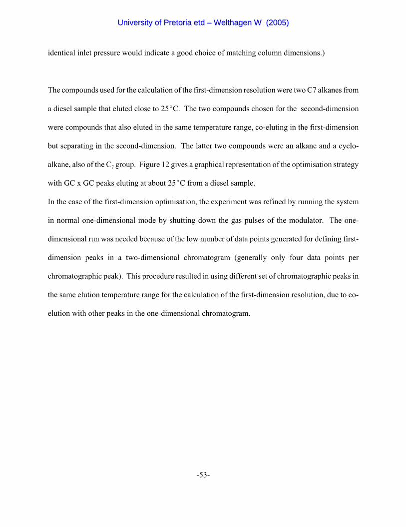
-53-
identical inlet pressure would indicate a good choice of matching column dimensions.)
The compounds used for the calculation of the first-dimension resolution were two C7 alkanes from
a diesel sample that eluted close to 25EC. The two compounds chosen for the second-dimension
were compounds that also eluted in the same temperature range, co-eluting in the first-dimension
but separating in the second-dimension. The latter two compounds were an alkane and a cyclo-
alkane, also of the C7 group. Figure 12 gives a graphical representation of the optimisation strategy
with GC x GC peaks eluting at about 25EC from a diesel sample.
In the case of the first-dimension optimisation, the experiment was refined by running the system
in normal one-dimensional mode by shutting down the gas pulses of the modulator. The one-
dimensional run was needed because of the low number of data points generated for defining first-
dimension peaks in a two-dimensional chromatogram (generally only four data points per
chromatographic peak). This procedure resulted in using different set of chromatographic peaks in
the same elution temperature range for the calculation of the first-dimension resolution, due to co-
elution with other peaks in the one-dimensional chromatogram.
UUnniivveerrssiittyy ooff PPrreettoorriiaa eettdd –– WWeelltthhaaggeenn WW ((22000055))
-54-
Fig. 12 Graphical representation of the optimisation strategy with GC x GC peaks eluting at
about 25EC from a diesel sample.
UUnniivveerrssiittyy ooff PPrreettoorriiaa eettdd –– WWeelltthhaaggeenn WW ((22000055))
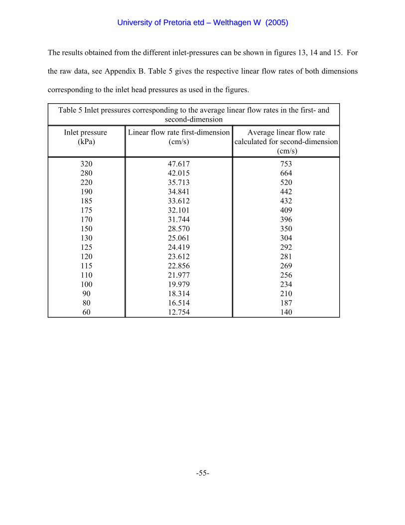
-55-
The results obtained from the different inlet-pressures can be shown in figures 13, 14 and 15. For
the raw data, see Appendix B. Table 5 gives the respective linear flow rates of both dimensions
corresponding to the inlet head pressures as used in the figures.
Table 5 Inlet pressures corresponding to the average linear flow rates in the first- andsecond-dimension
Inlet pressure (kPa)
Linear flow rate first-dimension(cm/s)
Average linear flow ratecalculated for second-dimension
(cm/s)320280220190185175170150130125120115110100908060
47.61742.01535.71334.84133.61232.10131.74428.57025.06124.41923.61222.85621.97719.97918.31416.51412.754
753664520442432409396350304292281269256234210187140
UUnniivveerrssiittyy ooff PPrreettoorriiaa eettdd –– WWeelltthhaaggeenn WW ((22000055))
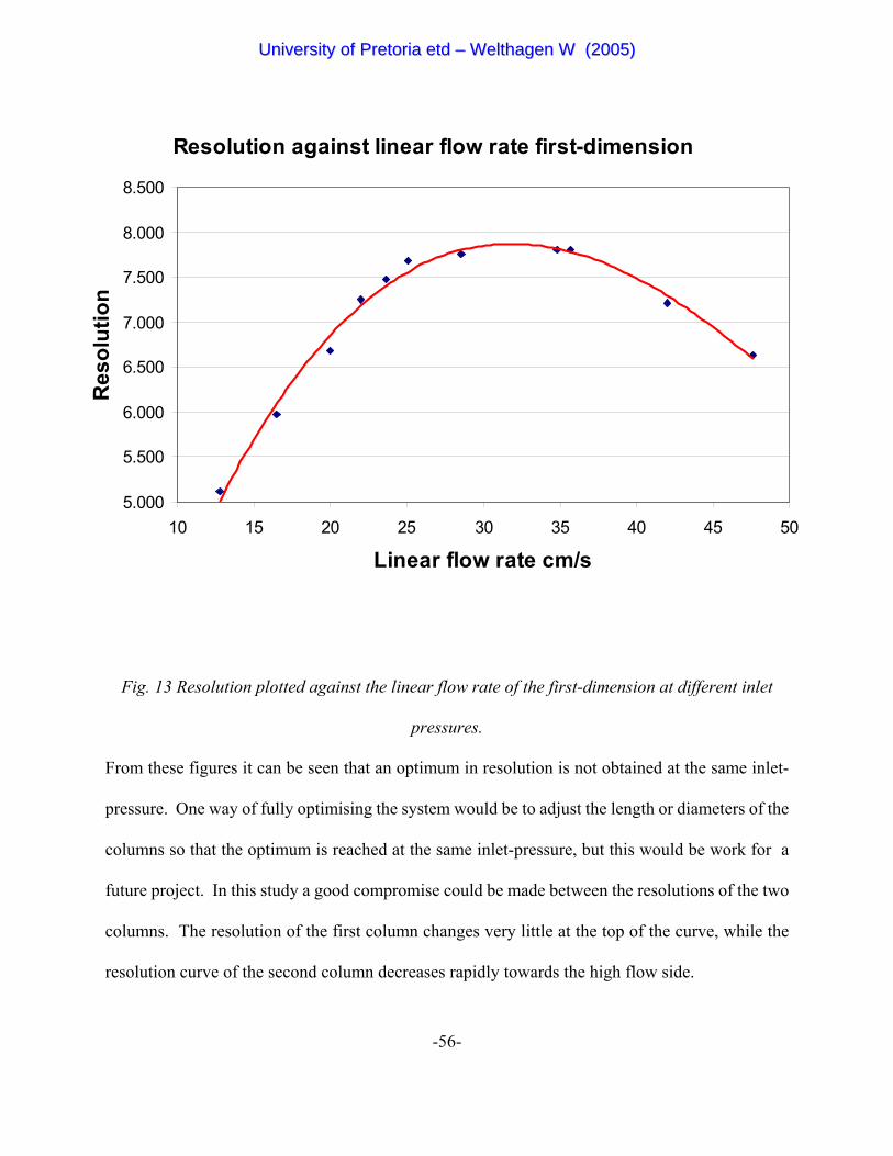
-56-
Resolution against linear flow rate first-dimension
5.000
5.500
6.000
6.500
7.000
7.500
8.000
8.500
10 15 20 25 30 35 40 45 50
Linear flow rate cm/s
Res
olut
ion
Fig. 13 Resolution plotted against the linear flow rate of the first-dimension at different inlet
pressures.
From these figures it can be seen that an optimum in resolution is not obtained at the same inlet-
pressure. One way of fully optimising the system would be to adjust the length or diameters of the
columns so that the optimum is reached at the same inlet-pressure, but this would be work for a
future project. In this study a good compromise could be made between the resolutions of the two
columns. The resolution of the first column changes very little at the top of the curve, while the
resolution curve of the second column decreases rapidly towards the high flow side.
UUnniivveerrssiittyy ooff PPrreettoorriiaa eettdd –– WWeelltthhaaggeenn WW ((22000055))
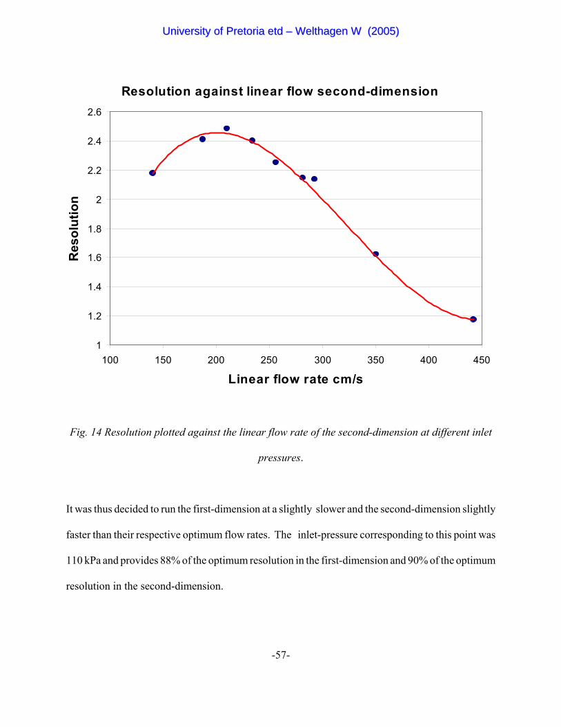
-57-
Resolution against linear flow second-dimension
1
1.2
1.4
1.6
1.8
2
2.2
2.4
2.6
100 150 200 250 300 350 400 450
Linear flow rate cm/s
Res
olut
ion
Fig. 14 Resolution plotted against the linear flow rate of the second-dimension at different inlet
pressures.
It was thus decided to run the first-dimension at a slightly slower and the second-dimension slightly
faster than their respective optimum flow rates. The inlet-pressure corresponding to this point was
110 kPa and provides 88% of the optimum resolution in the first-dimension and 90% of the optimum
resolution in the second-dimension.
UUnniivveerrssiittyy ooff PPrreettoorriiaa eettdd –– WWeelltthhaaggeenn WW ((22000055))
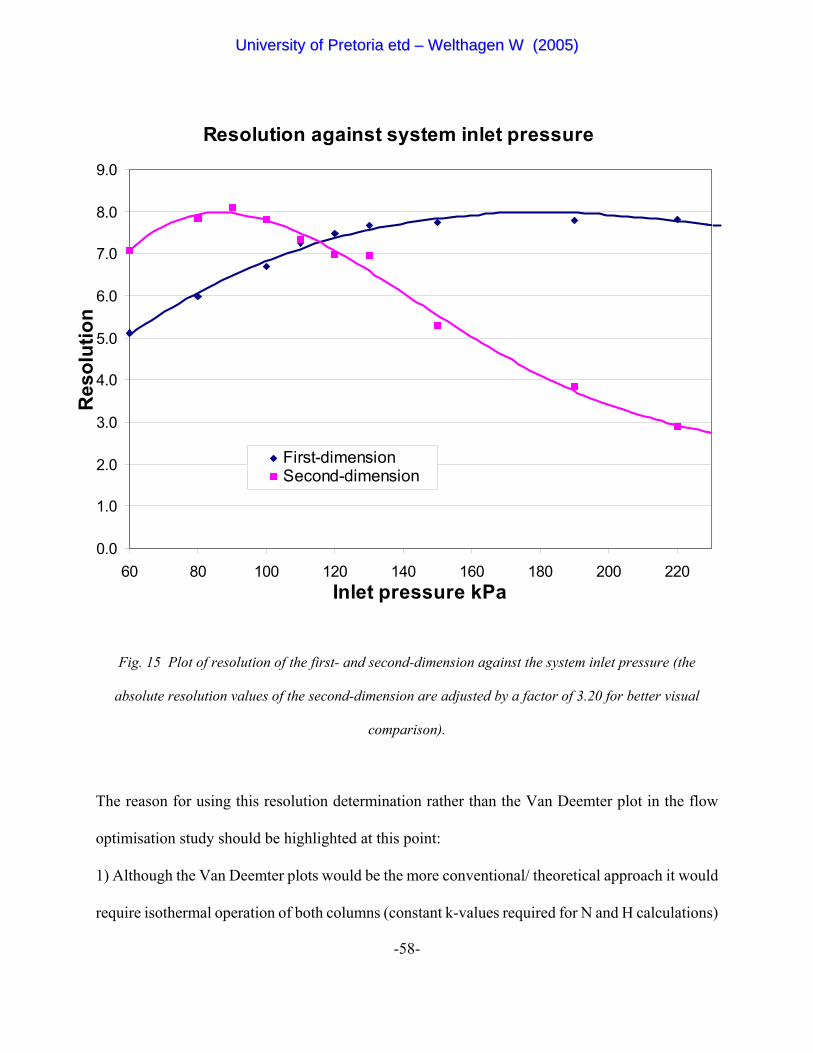
-58-
Resolution against system inlet pressure
0.0
1.0
2.0
3.0
4.0
5.0
6.0
7.0
8.0
9.0
60 80 100 120 140 160 180 200 220Inlet pressure kPa
Res
olut
ion
First-dimensionSecond-dimension
Fig. 15 Plot of resolution of the first- and second-dimension against the system inlet pressure (the
absolute resolution values of the second-dimension are adjusted by a factor of 3.20 for better visual
comparison).
The reason for using this resolution determination rather than the Van Deemter plot in the flow
optimisation study should be highlighted at this point:
1) Although the Van Deemter plots would be the more conventional/ theoretical approach it would
require isothermal operation of both columns (constant k-values required for N and H calculations)
UUnniivveerrssiittyy ooff PPrreettoorriiaa eettdd –– WWeelltthhaaggeenn WW ((22000055))
-59-
which is difficult to achieve in practise.
2) Resolution determinations are just as valid under the more practical temperature programming
conditions and do not require the determination of absolute retention times, which are not easily
obtained in the GCxGC system used in this study.
3) Referring to the resolution equation (see Chapter 3): Provided the α- and k-values for the two
peaks used do not change appreciably with flow rate, the resolution achieved will be directly related
to the plate number and plate height. Flow optimisation of the resolution method under these
circumstances would then be equivalent to plate height optimisation (Van Deemter plot)
4) In any event resolution optimisation as performed in this GCxGC study has more practical
importance, as it incorporates both columns and modulator performance.
This resolution optimisation strategy should, however, not be done without investigating potential
errors of interpretation. In this study a fixed temperature program in the first dimension was used.
This would result in the compounds used for the calculations eluting at slightly different
temperatures (and k-values) with the change in flow rate. The first-dimension elution temperature
is also of concern for the retention behaviour of the second column since the analysed compounds
are subsequently subjected to slightly different second-dimension column temperatures under
different flow rates. This variation in temperatures would slightly affect the k-values and possibly
the α-values with consequences on resolution as predicted by the resolution equation (Chapter 3),
but unrelated to the flow rates. Compounds of similar chemical nature were therefore chosen for
the calculations since these compounds do not produce significant changes in α-values with
temperature. The changes in α- and k-values with flow would both introduce changes to the
UUnniivveerrssiittyy ooff PPrreettoorriiaa eettdd –– WWeelltthhaaggeenn WW ((22000055))
-60-
resolution (R) values that are test compound related but not column performance (N) related, i.e.
cannot be ascribed to changes in longitudinal diffusion or slow radial equilibria. The slow
temperature program chosen in the first-dimension produces large elution k-values (the lowest k
values for a particular compound occur at their highest temperature in the column, i.e. at elution)
such that the k/(k+1) term approaches unity as depicted in Figure 10 (Chapter 3). Thus only slight
changes in α are likely to contribute to changes in resolution with flow rate in the first-dimension -
an effect suppressed by selecting two peaks that are chemically very similar, so that their relative
k values do not change much with temperature.
This is not true for the second-dimension, as fast GC is often performed at very small k-values (k
< 4). This more critical case is therefore dealt with in greater detail below:
In Tables 5 and 6 the k- and α-terms of the test compounds are calculated for the respective column
head pressures used. This requires determination of absolute retention times and linear flow rate.
In practise this is not done that easily as there is no trigger for the beginning of second-dimension
chromatograms and the absolute retention times of peaks are thus uncertain. This was also one of
the major considerations for using the more practical resolution approach since in this method only
relative retention times are required. With the calculated “dead time” (section 5.3.1) the absolute
retention times of the test compounds can be calculated. This was done by firstly adjusting the two-
dimensional contour plot so that the unretained compounds from the second-dimension (low boiling,
non polar compounds, i.e. the C3 and C4 alkanes) are on the zero position of the time axis. The
“dead time” is then added to this zero position to give absolute retention times.
UUnniivveerrssiittyy ooff PPrreettoorriiaa eettdd –– WWeelltthhaaggeenn WW ((22000055))
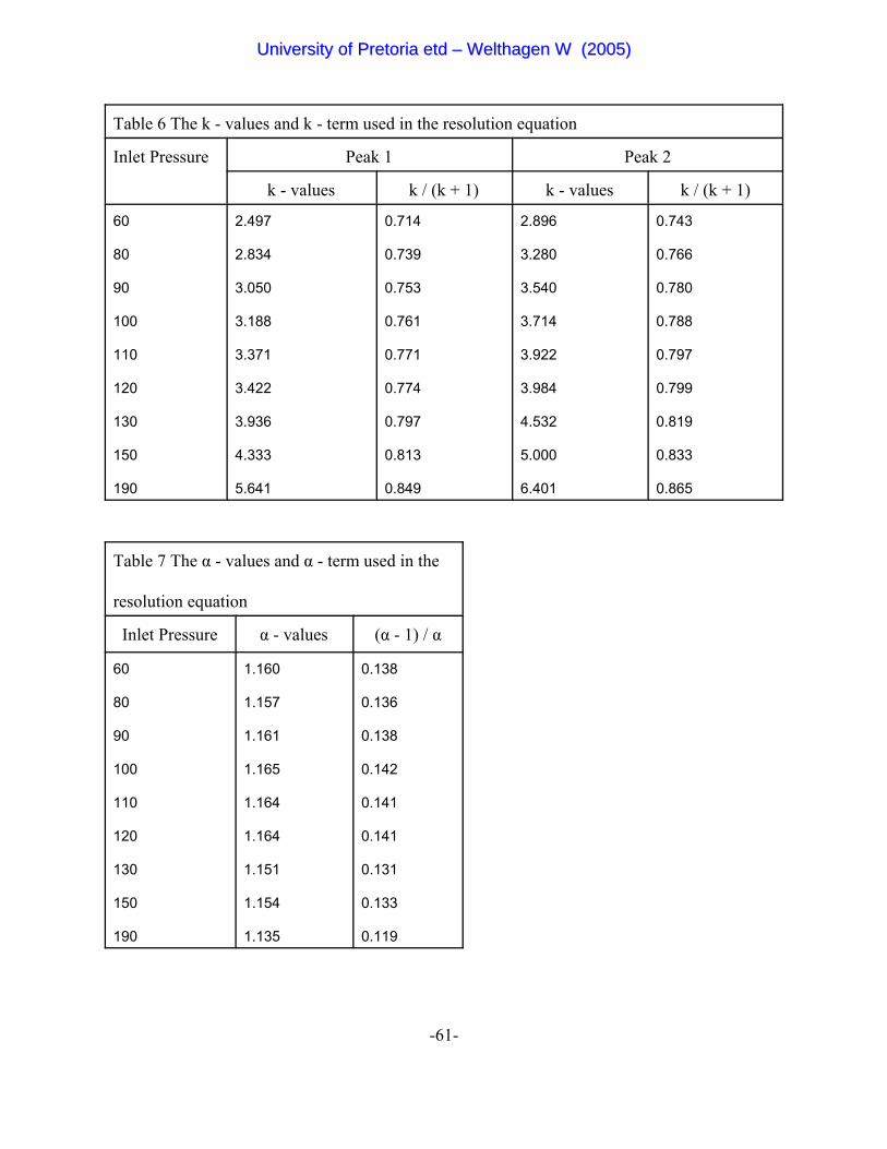
-61-
Table 6 The k - values and k - term used in the resolution equation
Inlet Pressure Peak 1 Peak 2
k - values k / (k + 1) k - values k / (k + 1)
60
80
90
100
110
120
130
150
190
2.497
2.834
3.050
3.188
3.371
3.422
3.936
4.333
5.641
0.714
0.739
0.753
0.761
0.771
0.774
0.797
0.813
0.849
2.896
3.280
3.540
3.714
3.922
3.984
4.532
5.000
6.401
0.743
0.766
0.780
0.788
0.797
0.799
0.819
0.833
0.865
Table 7 The α - values and α - term used in the
resolution equation
Inlet Pressure α - values (α - 1) / α
60
80
90
100
110
120
130
150
190
1.160
1.157
1.161
1.165
1.164
1.164
1.151
1.154
1.135
0.138
0.136
0.138
0.142
0.141
0.141
0.131
0.133
0.119
UUnniivveerrssiittyy ooff PPrreettoorriiaa eettdd –– WWeelltthhaaggeenn WW ((22000055))
-62-
As predicted the k-values (Table 6)are rather small and hence the k-term of the resolution equation
could vary a lot, but at the region of resolution optimum (i.e. 90 - 120 kPa) the k-term deviated
within a 2% (7% over the whole range measured). The α-terms (Table 7) have an even lower
deviation of only 2% over the total head-pressure range measured.
Whereas the resolution values (R) are also affected by the retention factors (k) and α value for the
test compounds, N values depend only the column performance as measured by N = (tr/σ)2.
Resolution values can be converted to N values once the k and α values of the test substances are
known. By rearrangement of the well known resolution equation (Chapter 3) we obtain:
N Rk
k=
+⎛⎝⎜
⎞⎠⎟ −⎛⎝⎜
⎞⎠⎟4
11
2 αα
The square root N values, thus calculated and presented in Figure 16, show that for our set of
second-dimension peaks (k •3), the optimisation in resolution and in column performance is found
at much the same inlet pressure/ linear flow rate. (Note that the optimum N value is found at a
marginally higher flow rate - justification for our theoretical concern over k and α values.) This
means that flow optimisation of the R value for the selected pair of compounds does indeed optimise
N values or column performance, obviating the need for the much more involved calculation of N
values that require absolute retention times.
UUnniivveerrssiittyy ooff PPrreettoorriiaa eettdd –– WWeelltthhaaggeenn WW ((22000055))

-63-
sqrt (N) against inlet pressure
0
10
20
30
40
50
60
70
80
90
100
50 70 90 110 130 150 170 190 210
Inlet pressure (kPa)
sqrt
(N)
Fig. 16 The plot of the square root of the plate number (N) against the inlet head pressure for the
evaluating the k- and α-term dependency of the resolution optimisation method
With absolute retention times known a second method of verification, the traditional Van Deemter
plot, can be done in the case of the second-dimension. This would be the fundamentally correct way
of column optimisation. Plate heights can be calculated by the following equation:
In practise, the equation found in Appendix B, based on the peak width at half height, is used.
UUnniivveerrssiittyy ooff PPrreettoorriiaa eettdd –– WWeelltthhaaggeenn WW ((22000055))
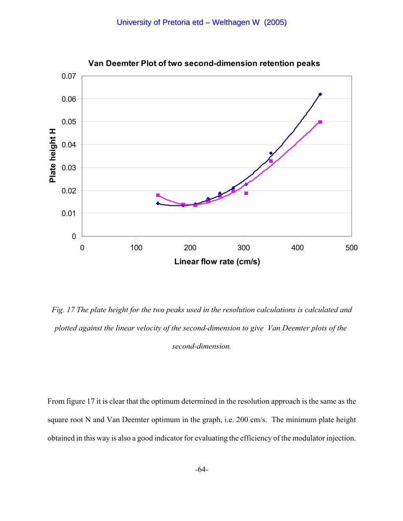
-64-
Van Deemter Plot of two second-dimension retention peaks
0
0.01
0.02
0.03
0.04
0.05
0.06
0.07
0 100 200 300 400 500
Linear flow rate (cm/s)
Plat
e he
ight
H
Fig. 17 The plate height for the two peaks used in the resolution calculations is calculated and
plotted against the linear velocity of the second-dimension to give Van Deemter plots of the
second-dimension.
From figure 17 it is clear that the optimum determined in the resolution approach is the same as the
square root N and Van Deemter optimum in the graph, i.e. 200 cm/s. The minimum plate height
obtained in this way is also a good indicator for evaluating the efficiency of the modulator injection.
UUnniivveerrssiittyy ooff PPrreettoorriiaa eettdd –– WWeelltthhaaggeenn WW ((22000055))
-65-
The Van Deemter plot shows a much steeper gradient of the curve in the fast linear flow rate region
than what is expected for a 100 Fm column (see figure 11). Together with the minimum plate height
that is about 35% higher than theoretically predicted for the 100 Fm i.d. column, this indicates that
the modulator injection into the second-dimension still has a negative contribution to overall system
performance. This contribution (σi) has an enhanced effect at higher flow rates, where compounds
elute with narrower peaks in time.
[22]HLN
Lt
t
r= =
⎛⎝⎜
⎞⎠⎟
σ2
[16]σ σ σt col inj2 2 2= +
This would result in larger H values at higher flow rates (lower tr) as σt/tr will increase. The result
is a steeper flow dependant curve than expected from pure column considerations. Indeed it can be
speculated that σinj could even increase with flow rate due to cooling effect of the higher internal
carrier gas flow.
The result of the flow optimisation study shows up the danger of blindly using literature Van
Deemter [52,53] results or generally accepted optimum flow rates for a specific inner diameter
column.
In figure 18 a comparison of using the generally accepted linear flow rate (40 cm/s) and the new
recommended linear flow rate (22 cm/s). From the two diesel chromatograms in figure 18, it is
UUnniivveerrssiittyy ooff PPrreettoorriiaa eettdd –– WWeelltthhaaggeenn WW ((22000055))
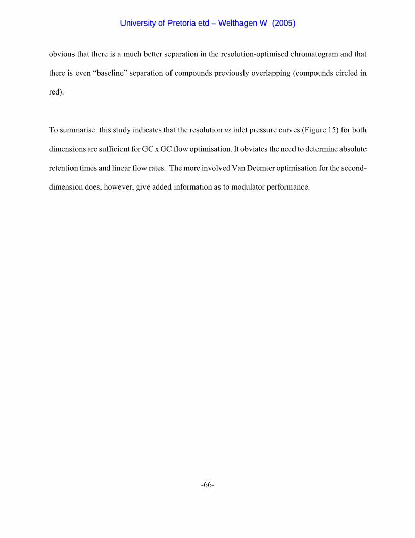
-66-
obvious that there is a much better separation in the resolution-optimised chromatogram and that
there is even “baseline” separation of compounds previously overlapping (compounds circled in
red).
To summarise: this study indicates that the resolution vs inlet pressure curves (Figure 15) for both
dimensions are sufficient for GC x GC flow optimisation. It obviates the need to determine absolute
retention times and linear flow rates. The more involved Van Deemter optimisation for the second-
dimension does, however, give added information as to modulator performance.
UUnniivveerrssiittyy ooff PPrreettoorriiaa eettdd –– WWeelltthhaaggeenn WW ((22000055))
-67-
R = 0.99
18
20
22
24
26
28
301 1.5 2 2.5 3
Second-dimension (s)
Firs
t-dim
ensi
on (m
in)
53 Peaks
Extract of a diesel chromatogram with linear flow rate of 40 cm/s
R = 1.77
22
24
26
28
30
32
341.2 1.7 2.2 2.7 3.2
Second-dimension (s)
Firs
t-dim
ensi
on (m
in)
68 Peaks
Extract of a diesel chromatogram with linear flow rate of 22 cm/s
Fig. 18 A comparison between diesel chromatograms using the generally accepted linear flow
rate of 40 cm/s for the first-dimension and the optimised linear flow rate of 22 cm/s.
UUnniivveerrssiittyy ooff PPrreettoorriiaa eettdd –– WWeelltthhaaggeenn WW ((22000055))
-68-
5.3.3 Choice of second dimension stationary phase
The choice of a stationary phase in chromatographic separations generally depends on the type of
separations required and the type of sample to be analysed (see discussion on dimensionality
Chapter 2). As discussed in Chapter 3 the two different stationary phases used in this study were
a PEG column and 17% cyanopropylphenyl - 83% dimethyl polysiloxane column. The PEG column
which is quite a polar column is in principle the best phase to provide “polarity” separation (see
orthogonality consideration Chapter 2). The PEG column can separate compounds of different
polarity with great efficiency, but the time required to separate these compounds becomes
increasingly long as the polarity range of compounds in a sample increases. The second-dimension,
however, has a limited time allowed for the compounds to elute. For the most polar compounds to
elute within the fixed time frame (modulation period) the column is run at higher temperatures,
which result in compounds eluting early in the chromatogram to be “squashed” together (lower R
values at too low k values). This behaviour is referred to as the general elution problem (section
3.2.4). In principle, temperature programming in the second-dimension will solve this problem; a
technology not yet available for the fast, repetitive second-dimension. Presently the PEG column
is probably best reserved for samples containing compounds in a narrow polarity range.
The use of a less polar column like the 17% cyanopropylphenyl - 83% dimethyl polysiloxane
column allows a lower temperature separation and decreased “squashing” of early eluting peaks.
The separation of different polarity classes obtained with this column is less than that of the PEG
column. The 17% cyanopropylphenyl - 83% dimethyl polysiloxane column can, however, separate
UUnniivveerrssiittyy ooff PPrreettoorriiaa eettdd –– WWeelltthhaaggeenn WW ((22000055))
-69-
compounds eluting early (i.e. alkanes and cycloalkanes) in the chromatogram much more efficiently.
The eventual aim of this study was to investigate potential applications for the analysis of diesel
samples, which contain mostly compounds of low polarity alkanes and cyclic alkanes, as well as
some medium polar (mono-aromatic, di-aromatic and tri-aromatic) compounds.. The 17%
cyanopropylphenyl - 83% dimethyl polysiloxane column proved to be more robust in that it seemed
to have a much longer life time than the PEG column. Both columns had an upper temperature limit
of 270EC but the PEG column required operation at or above its recommended maximum
temperature when diesel samples were analysed at higher temperatures (higher temperatures to get
the compounds to elude in the defined modulation period). The 17% cyanopropylphenyl - 83%
dimethyl polysiloxane column was, therefore, the column of choice in this optimisation study.
In figure 19 a comparison between the two different columns can be seen. From these figures some
of the above concerns for not using the PEG becomes more apparent. In the accompanying
extraction sections of the figures it can be clearly seen that the PEG column is able to separate
compounds with great efficiency, but can do so only in specific narrow polarity ranges (in the case
presented here it was best suited for separating the aromatic bands and thus the alkane and cyclo-
alkane bands is “squashed” together, small k-values), the cyanopropylphenyl column on the other
hand provides a more even separation of all the compound groups analysed (k-values bigger than
three).
UUnniivveerrssiittyy ooff PPrreettoorriiaa eettdd –– WWeelltthhaaggeenn WW ((22000055))
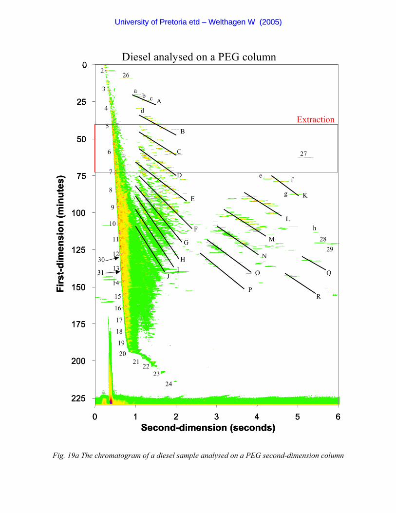
0
25
50
75
100
125
150
175
200
225
0 1 2 3 4 5 6Second-dimension (seconds)
Firs
t-dim
ensi
on (m
inut
es)
Diesel analysed on a PEG column
Extraction
262
3
4
5
6
7
8
A
27
9
10
11
12
13
14
15
16
17
18
1920
2122
2324
30
31
2829
Q
R
B
C
D
E
F
G
HI
J
K
L
M
N
O
P
ab c
d
ef
g
h
0
25
50
75
100
125
150
175
200
225
0 1 2 3 4 5 6Second-dimension (seconds)
Firs
t-dim
ensi
on (m
inut
es)
Diesel analysed on a PEG column
Extraction
262
3
4
5
6
7
8
A
27
9
10
11
12
13
14
15
16
17
18
1920
2122
2324
30
31
2829
Q
R
B
C
D
E
F
G
HI
J
K
L
M
N
O
P
0
25
50
75
100
125
150
175
200
225
0 1 2 3 4 5 6Second-dimension (seconds)
Firs
t-dim
ensi
on (m
inut
es)
Diesel analysed on a PEG column
Extraction
262
3
4
5
6
7
8
A
27
9
10
11
12
13
14
15
16
17
18
1920
2122
2324
30
31
2829
Q
R
B
C
D
E
F
G
HI
J
K
L
M
N
O
P
ab c
d
ef
g
h
Fig. 19a The chromatogram of a diesel sample analysed on a PEG second-dimension column
UUnniivveerrssiittyy ooff PPrreettoorriiaa eettdd –– WWeelltthhaaggeenn WW ((22000055))
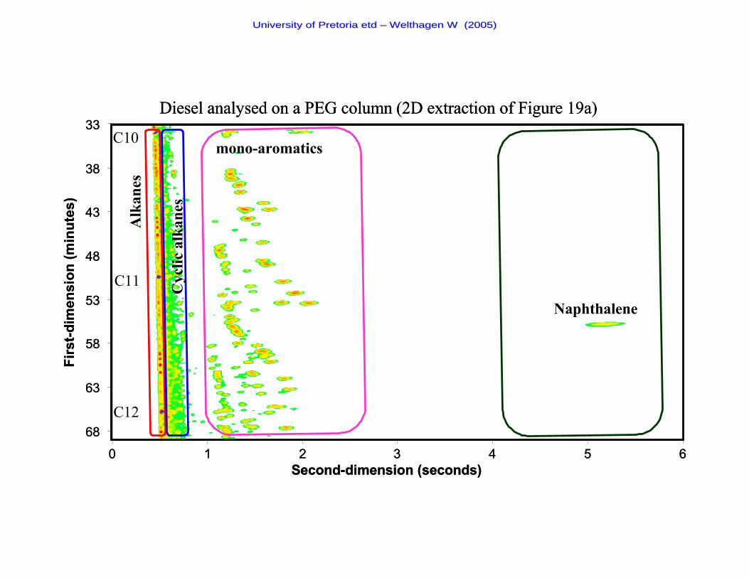
33
38
43
48
53
58
63
68
0 1 2 3 4 5 6Second-dimension (seconds)
Firs
t-dim
ensi
on (m
inut
es)
Diesel analysed on a PEG column (2D extraction of Figure 19a)
C11
C12
C10
Naphthalene
Alk
anes
Cyc
lic a
lkan
es
mono-aromatics33
38
43
48
53
58
63
68
0 1 2 3 4 5 6Second-dimension (seconds)
Firs
t-dim
ensi
on (m
inut
es)
Diesel analysed on a PEG column (2D extraction of Figure 19a)
C11
C12
C10
Naphthalene
Alk
anes
Cyc
lic a
lkan
es
mono-aromatics
UUnniivveerrssiittyy ooff PPrreettoorriiaa eettdd –– WWeelltthhaaggeenn WW ((22000055))
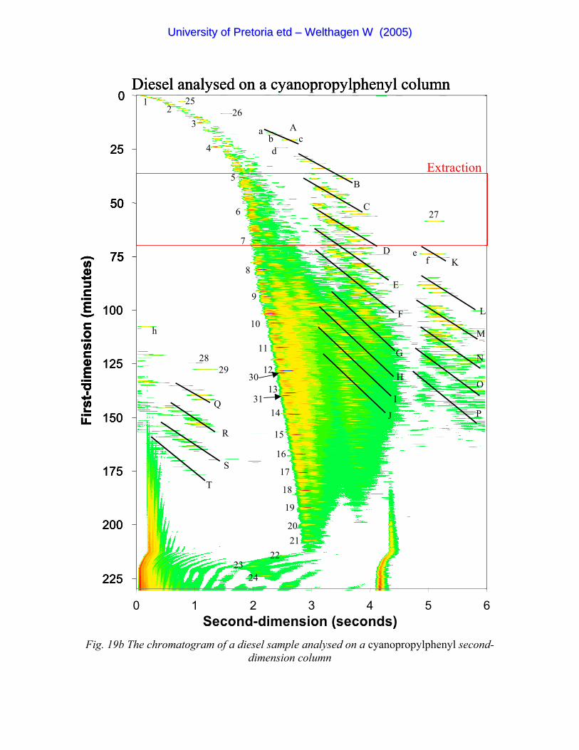
0
25
50
75
100
125
150
175
200
225
0 1 2 3 4 5 6Second-dimension (seconds)
Firs
t-dim
ensi
on (m
inut
es)
Diesel analysed on a cyanopropylphenyl column
50
75
Extraction
25262
3
4
5
6
7
8
A
27
1
9
10
11
12
13
14
15
16
17
18
19
2021
2223
24
30
31
2829
Q
R
S
T
B
C
D
E
F
G
H
I
J
K
L
M
N
O
P
ab cd
ef
h
0
25
50
75
100
125
150
175
200
225
0 1 2 3 4 5 6Second-dimension (seconds)
Firs
t-dim
ensi
on (m
inut
es)
Diesel analysed on a cyanopropylphenyl column
50
75
Extraction
25262
3
4
5
6
7
8
A
27
1
9
10
11
12
13
14
15
16
17
18
19
2021
2223
24
30
31
2829
Q
R
S
T
B
C
D
E
F
G
H
I
J
K
L
M
N
O
P
0
25
50
75
100
125
150
175
200
225
0 1 2 3 4 5 6Second-dimension (seconds)
Firs
t-dim
ensi
on (m
inut
es)
Diesel analysed on a cyanopropylphenyl column
50
75
Extraction
25262
3
4
5
6
7
8
A
27
1
9
10
11
12
13
14
15
16
17
18
19
2021
2223
24
30
31
2829
Q
R
S
T
B
C
D
E
F
G
H
I
J
K
L
M
N
O
P
ab cd
ef
h
Fig. 19b The chromatogram of a diesel sample analysed on a cyanopropylphenyl second-dimension column
UUnniivveerrssiittyy ooff PPrreettoorriiaa eettdd –– WWeelltthhaaggeenn WW ((22000055))
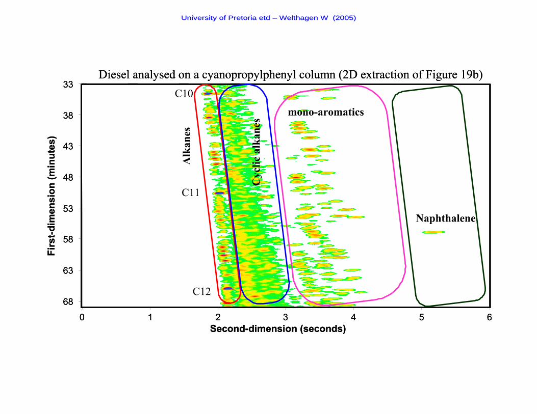
33
38
43
48
53
58
63
68
0 1 2 3 4 5 6Second-dimension (seconds)
Firs
t-dim
ensi
on (m
inut
es)
Diesel analysed on a cyanopropylphenyl column (2D extraction of Figure 19b)
Naphthalene
C11
C12
C10
Alk
anes
Cyc
lic a
lkan
es
mono-aromatics
33
38
43
48
53
58
63
68
0 1 2 3 4 5 6Second-dimension (seconds)
Firs
t-dim
ensi
on (m
inut
es)
Diesel analysed on a cyanopropylphenyl column (2D extraction of Figure 19b)
Naphthalene
C11
C12
C10
Alk
anes
Cyc
lic a
lkan
es
mono-aromatics
UUnniivveerrssiittyy ooff PPrreettoorriiaa eettdd –– WWeelltthhaaggeenn WW ((22000055))
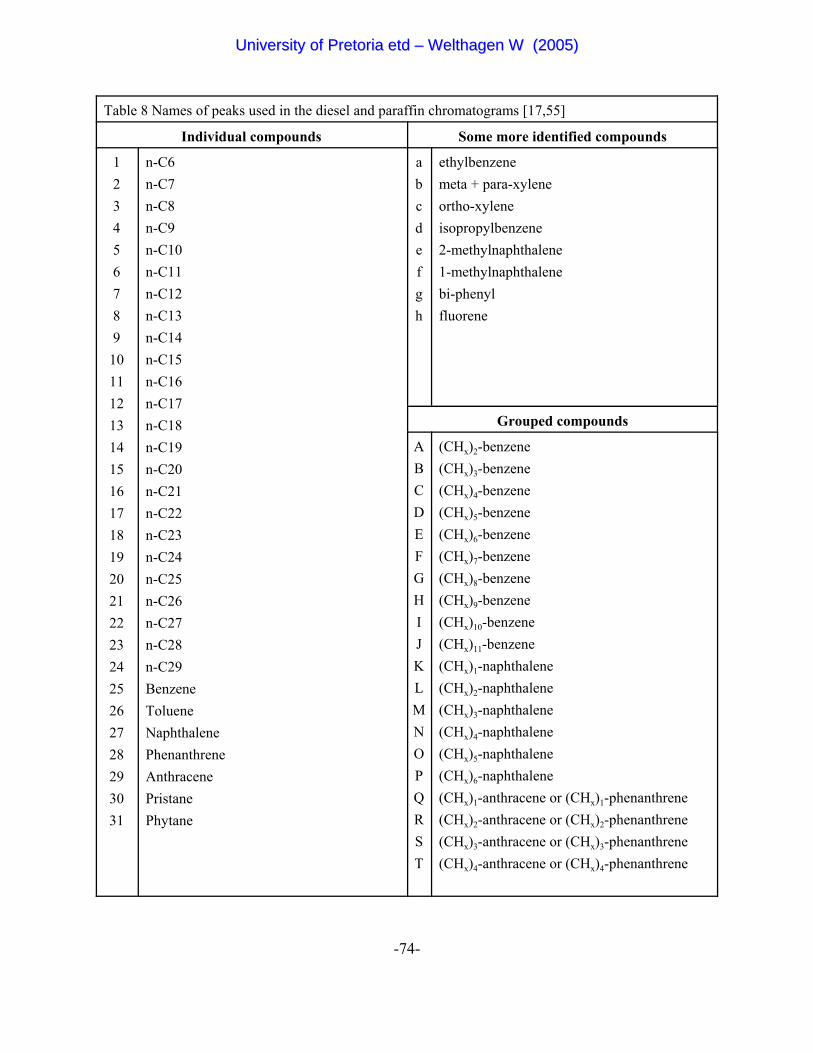
-74-
Table 8 Names of peaks used in the diesel and paraffin chromatograms [17,55]
Individual compounds Some more identified compounds
123456789
10111213141516171819202122232425262728293031
n-C6n-C7n-C8n-C9n-C10n-C11n-C12n-C13n-C14n-C15n-C16n-C17n-C18n-C19n-C20n-C21n-C22n-C23n-C24n-C25n-C26n-C27n-C28n-C29BenzeneTolueneNaphthalenePhenanthreneAnthracenePristanePhytane
abcdefgh
ethylbenzenemeta + para-xyleneortho-xyleneisopropylbenzene2-methylnaphthalene1-methylnaphthalenebi-phenylfluorene
Grouped compounds
ABCDEFGHIJKLMNOPQRST
(CHx)2-benzene(CHx)3-benzene(CHx)4-benzene(CHx)5-benzene(CHx)6-benzene(CHx)7-benzene(CHx)8-benzene(CHx)9-benzene(CHx)10-benzene(CHx)11-benzene(CHx)1-naphthalene(CHx)2-naphthalene(CHx)3-naphthalene(CHx)4-naphthalene(CHx)5-naphthalene(CHx)6-naphthalene(CHx)1-anthracene or (CHx)1-phenanthrene (CHx)2-anthracene or (CHx)2-phenanthrene(CHx)3-anthracene or (CHx)3-phenanthrene(CHx)4-anthracene or (CHx)4-phenanthrene
UUnniivveerrssiittyy ooff PPrreettoorriiaa eettdd –– WWeelltthhaaggeenn WW ((22000055))
-75-
5.3.4 Temperature difference between the columns
From section 5.3.3 it is obvious that there are specific temperatures required for fast second-
dimension separation. The second-dimension is operated at a constant temperature difference with
the first-dimension temperature. The temperature difference depends on the sample used, the
dimensions and the stationary-phase of the second-dimension column. In our case we never changed
the column dimensions. The optimisation of the temperature difference has to take the following
into consideration: The modulation period (time allowed for each second-dimension chromatogram)
is predefined by the temperature program of the first-dimension as this will dictate the time-width
of the peaks eluting from the first-dimension. This first-dimension peak has to be analysed several
times by the second-dimension column, a generally accepted number of cuts being four over each
first-dimension peak. For a temperature program of 1EC/min, providing ca. 30 s first-dimension
peak widths, the preferred second-dimension time is five to six seconds.
The temperature of the second-dimension column now needs to be adjusted in order to fully utilise
this predefined time. The temperature thus needs to be low enough to allow the compounds to
separate, but high enough (large enough k value, see Figure 10) not to stay in the column too long
to co-elute with the next second-dimension portion (“wrap-around”, figure 20). The temperature
should be selected for the peaks to elute over the full separation time. For the PEG column the
optimum temperature difference when analysing diesel was observed to be 30EC and that of the 17%
cyanopropylphenyl - 83% dimethyl polysiloxane column to be 20EC higher than the first-dimension
temperature.
UUnniivveerrssiittyy ooff PPrreettoorriiaa eettdd –– WWeelltthhaaggeenn WW ((22000055))
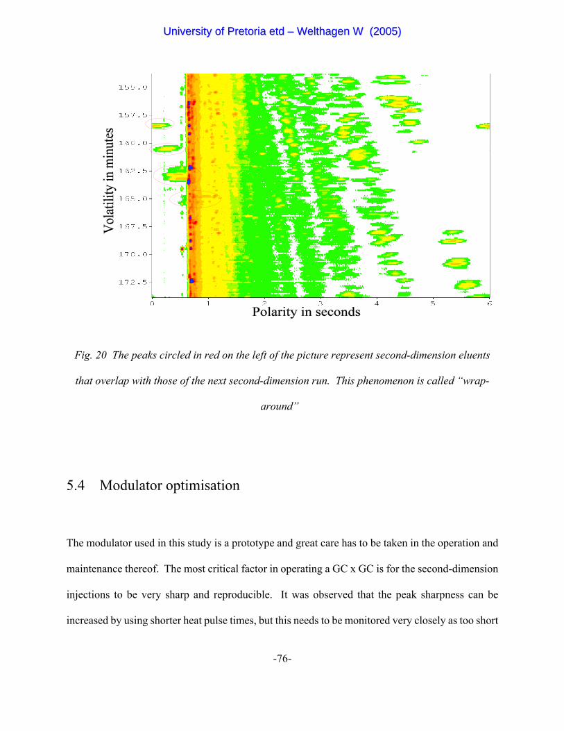
-76-
Fig. 20 The peaks circled in red on the left of the picture represent second-dimension eluents
that overlap with those of the next second-dimension run. This phenomenon is called “wrap-
around”
5.4 Modulator optimisation
The modulator used in this study is a prototype and great care has to be taken in the operation and
maintenance thereof. The most critical factor in operating a GC x GC is for the second-dimension
injections to be very sharp and reproducible. It was observed that the peak sharpness can be
increased by using shorter heat pulse times, but this needs to be monitored very closely as too short
UUnniivveerrssiittyy ooff PPrreettoorriiaa eettdd –– WWeelltthhaaggeenn WW ((22000055))
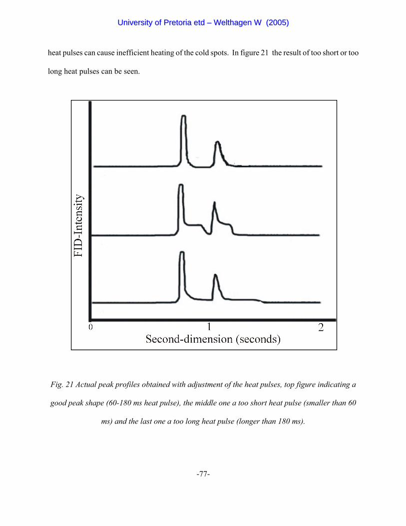
-77-
heat pulses can cause inefficient heating of the cold spots. In figure 21 the result of too short or too
long heat pulses can be seen.
Fig. 21 Actual peak profiles obtained with adjustment of the heat pulses, top figure indicating a
good peak shape (60-180 ms heat pulse), the middle one a too short heat pulse (smaller than 60
ms) and the last one a too long heat pulse (longer than 180 ms).
UUnniivveerrssiittyy ooff PPrreettoorriiaa eettdd –– WWeelltthhaaggeenn WW ((22000055))
-78-
The step that is formed in the middle chromatogram (behind the short heat pulse peak) indicates that
not all of the eluent trapped on the cold spot is injected at once and the rest is injected in a delayed
step. The sharp decline at the end of the step indicates that the cold jet has been reactivated and is
cooling the spot down, trapping the remainder of the eluent that should have been injected if the
pulse was of sufficient heat. The too long heat pulse has a similar effect but now unmodulated
eluents from the first-dimension column are starting to move through the trap due to the trap being
too warm for the cold jets to trap this eluent. The sharpest peak shapes were found when using a
heat pulse of between 60 ms and 180 ms. The longer pulse was chosen due to some weather related
effects discussed later.
The effect of using an increased gas pulse pressure was also examined. The increase of the gas
pressure in the hot jets worked effectively at oven temperatures below 150EC but at higher oven
temperatures the results were negatively affected. The negative effect was due to a too short heating
section in the modulator for the larger volume hot pulses and thus resulting in pulsing cooler gas
onto the cold spot than required to remobilise the trapped compounds. The last portion of the hot
pulse volume comes from outside the GC oven and indeed cools the trapped area too below the oven
temperature. As a modification to the modulator it would therefore be advised to use a longer
heating section (e.g. an additional 0.5 m of a metal tube being inside the oven) so that a larger
amount of hot gas can be blown onto the cold spot in a shorter time-frame.
During a period of high humidity in the laboratory it was noticed that the cold spots would condense
water from the atmosphere and cause ice formation. The ice collecting on the column has a much
higher thermal capacity, resulting in the heat pulses being inefficient in remobilising the eluents
UUnniivveerrssiittyy ooff PPrreettoorriiaa eettdd –– WWeelltthhaaggeenn WW ((22000055))
-79-
trapped in the cold zones. This inefficiency ranged from increased peak widths to permanent
trapping of eluents. In a first attempt to reduce this effect, a lower cold flow pressure was used to
just trap any first column eluents. This reduction in cold flow rates worked quite well at higher oven
temperatures, but at lower temperatures it was ineffective in trapping the more volatile eluents. To
utilise these reduced cold flow rates, different flow stages thus had to be defined for the cold flow.
At temperatures below 10EC a cold flow of above 40 ml/min is needed, between 10EC and 40EC
a flow of 30 ml/min was effective and above 40EC the cold flow can be reduced to 20 or 15 ml/min.
The reduced cold flow rates helped a lot in decreasing ice formation above 40EC but at lower
temperatures other precautions had to be taken: The oven was cryogenically cooled to 10EC and
lower with liquid nitrogen, to reduce the water content of the oven atmosphere. As the liquid
nitrogen evaporates it displaces the humid atmospheric air from the GC oven. In normal cool down
mode the oven vents open for faster cooling with laboratory air, also during the initial stages of the
GC run when the cold jets of the modulator start to operate and freeze out laboratory moisture on
the cold spots of the modulator. As a further precaution silica gel was placed inside the oven and
the oven vents were sealed with aluminium foil to keep the moisture levels down during instrument-
down periods. These precaution measures have shown great improvement in modulator operation,
in that the cold spots did not freeze up under these conditions, and that even lower flows (about 10
ml/min, compared to 20 ml/min without the precautions) of cold nitrogen air were required to
efficiently trap the compounds eluting from the first-dimension column. From a cost point of view,
this is of course, a great improvement.
UUnniivveerrssiittyy ooff PPrreettoorriiaa eettdd –– WWeelltthhaaggeenn WW ((22000055))
-80-
Chapter 6
Analysis of diesel petroleum fractions
Table of Contents
6.1 Introduction
6.2 Experimental setup
6.3 The analysis of four local diesel samples
6.4 The analysis of diesel-paraffin mixtures
UUnniivveerrssiittyy ooff PPrreettoorriiaa eettdd –– WWeelltthhaaggeenn WW ((22000055))
-81-
Chapter 6
Analysis of diesel petroleum fractions
6.1 Introduction
The analysis of petroleum products is already well established and done routinely in many
laboratories. The different techniques involved in the analysis of petroleum fractions are discussed
in Chapter 4. In Chapter 4 it is also mentioned that GC x GC can be used as a valuable tool in the
analysis of these samples. This section of the dissertation investigates the fingerprinting of different
diesel samples. The eventual use of this fingerprinting technique would be to accurately identify
diesel in pollution and arson studies.
A few interesting samples of specialist diesels were also examined for their differences in lubricating
efficiencies. These samples were obtained from the Mechanical Engineering Department of the
University of Pretoria and contained different diesel-paraffin mixtures used in the South African
mining industry.
At the time of this study, no two-dimensional automated peak integration software for GC x GC was
available, therefore, the fingerprinting and sample comparisons were done on a visual interpretation
UUnniivveerrssiittyy ooff PPrreettoorriiaa eettdd –– WWeelltthhaaggeenn WW ((22000055))
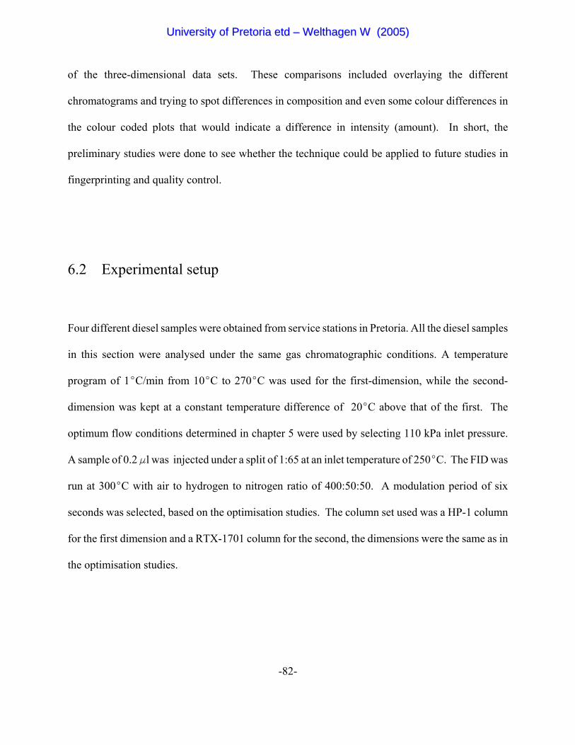
-82-
of the three-dimensional data sets. These comparisons included overlaying the different
chromatograms and trying to spot differences in composition and even some colour differences in
the colour coded plots that would indicate a difference in intensity (amount). In short, the
preliminary studies were done to see whether the technique could be applied to future studies in
fingerprinting and quality control.
6.2 Experimental setup
Four different diesel samples were obtained from service stations in Pretoria. All the diesel samples
in this section were analysed under the same gas chromatographic conditions. A temperature
program of 1EC/min from 10EC to 270EC was used for the first-dimension, while the second-
dimension was kept at a constant temperature difference of 20EC above that of the first. The
optimum flow conditions determined in chapter 5 were used by selecting 110 kPa inlet pressure.
A sample of 0.2 Fl was injected under a split of 1:65 at an inlet temperature of 250EC. The FID was
run at 300EC with air to hydrogen to nitrogen ratio of 400:50:50. A modulation period of six
seconds was selected, based on the optimisation studies. The column set used was a HP-1 column
for the first dimension and a RTX-1701 column for the second, the dimensions were the same as in
the optimisation studies.
UUnniivveerrssiittyy ooff PPrreettoorriiaa eettdd –– WWeelltthhaaggeenn WW ((22000055))
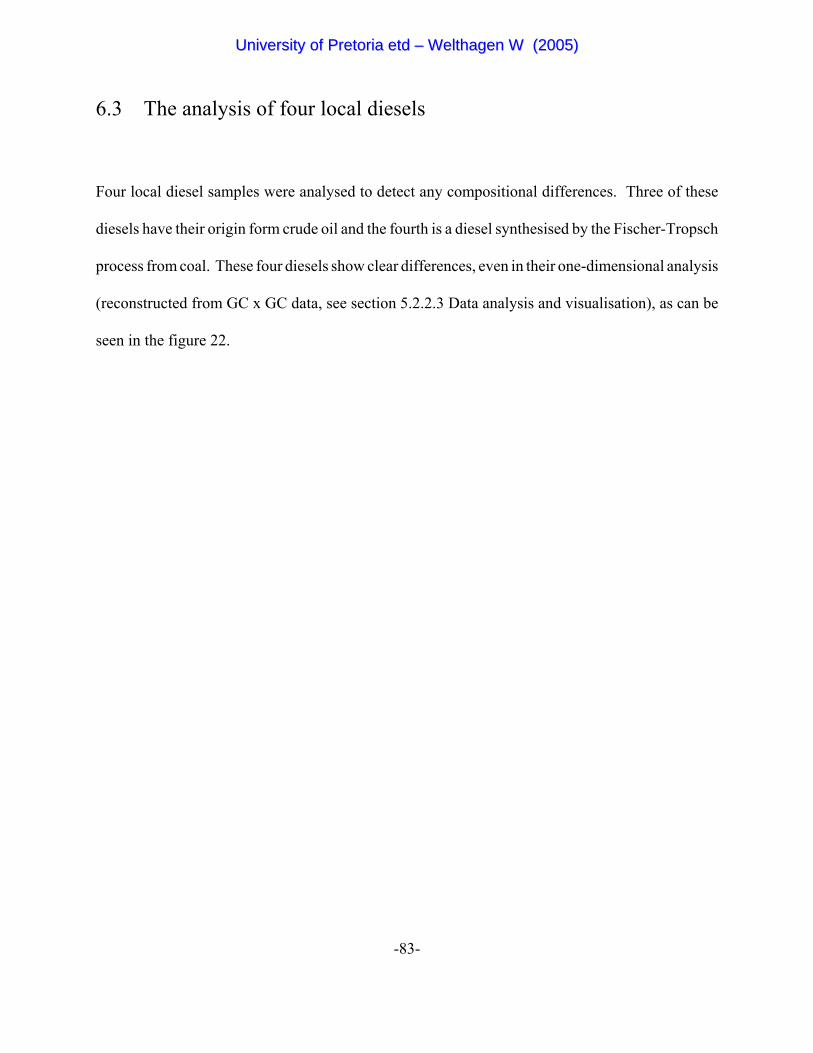
-83-
6.3 The analysis of four local diesels
Four local diesel samples were analysed to detect any compositional differences. Three of these
diesels have their origin form crude oil and the fourth is a diesel synthesised by the Fischer-Tropsch
process from coal. These four diesels show clear differences, even in their one-dimensional analysis
(reconstructed from GC x GC data, see section 5.2.2.3 Data analysis and visualisation), as can be
seen in the figure 22.
UUnniivveerrssiittyy ooff PPrreettoorriiaa eettdd –– WWeelltthhaaggeenn WW ((22000055))
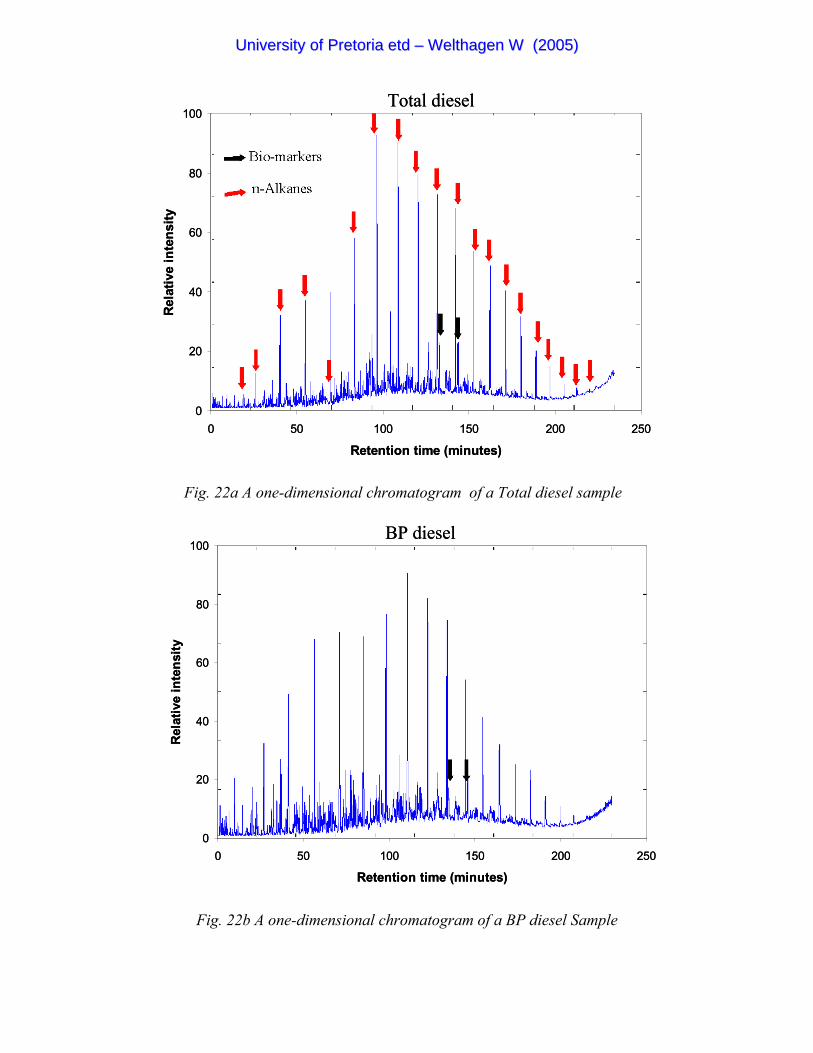
0
20
40
60
80
100
0 50 100 150 200 250
Retention time (minutes)
Rel
ativ
e in
tens
ity
Total diesel
0
20
40
60
80
100
0 50 100 150 200 250
Retention time (minutes)
Rel
ativ
e in
tens
ity
Total diesel
0
20
40
60
80
100
0 50 100 150 200 250
Retention time (minutes)
Rel
ativ
e in
tens
ity
BP diesel
0
20
40
60
80
100
0 50 100 150 200 250
Retention time (minutes)
Rel
ativ
e in
tens
ity
BP diesel
Fig. 22a A one-dimensional chromatogram of a Total diesel sample
Fig. 22b A one-dimensional chromatogram of a BP diesel Sample
UUnniivveerrssiittyy ooff PPrreettoorriiaa eettdd –– WWeelltthhaaggeenn WW ((22000055))
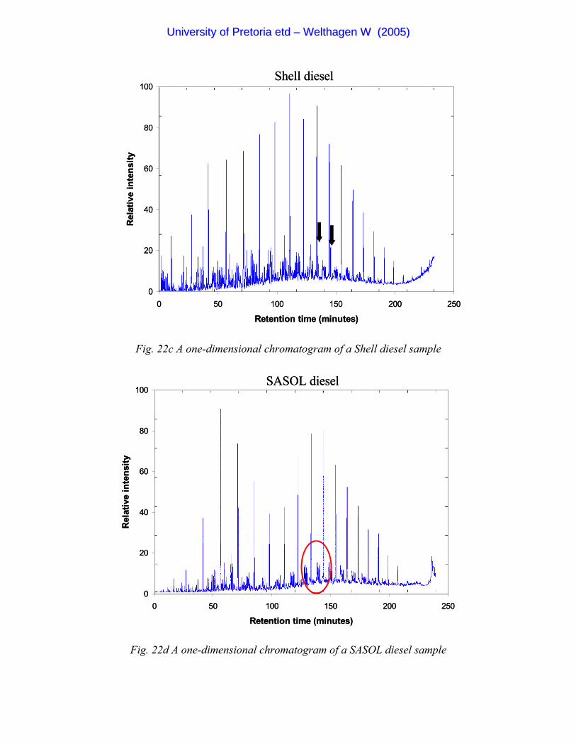
0
20
40
60
80
100
0 50 100 150 200 250
Retention time (minutes)
Rel
ativ
e in
tens
ity
Shell diesel
0
20
40
60
80
100
0 50 100 150 200 250
Retention time (minutes)
Rel
ativ
e in
tens
ity
Shell diesel
0
20
40
60
80
100
0 50 100 150 200 250
Retention time (minutes)
Rel
ativ
e in
tens
ity
SASOL diesel
0
20
40
60
80
100
0 50 100 150 200 250
Retention time (minutes)
Rel
ativ
e in
tens
ity
SASOL diesel
Fig. 22c A one-dimensional chromatogram of a Shell diesel sample
Fig. 22d A one-dimensional chromatogram of a SASOL diesel sample
UUnniivveerrssiittyy ooff PPrreettoorriiaa eettdd –– WWeelltthhaaggeenn WW ((22000055))
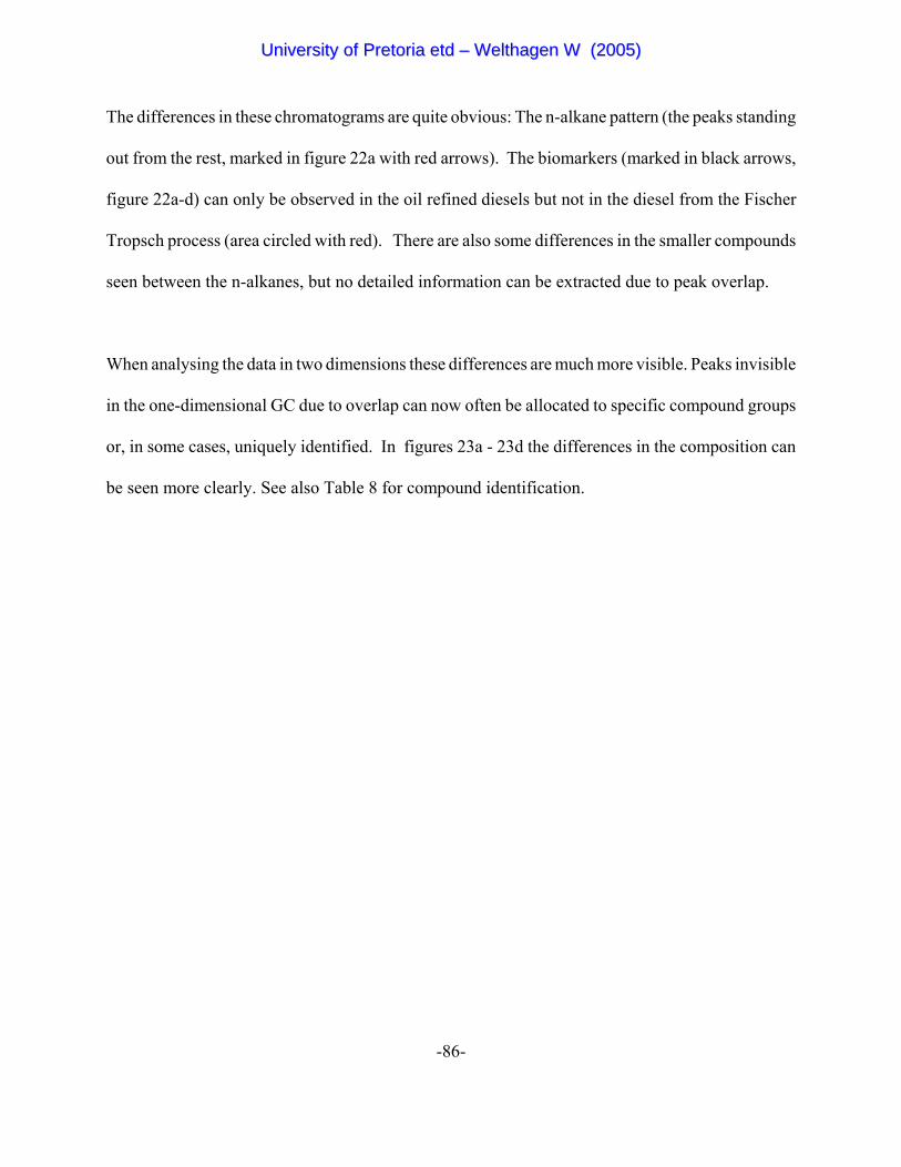
-86-
The differences in these chromatograms are quite obvious: The n-alkane pattern (the peaks standing
out from the rest, marked in figure 22a with red arrows). The biomarkers (marked in black arrows,
figure 22a-d) can only be observed in the oil refined diesels but not in the diesel from the Fischer
Tropsch process (area circled with red). There are also some differences in the smaller compounds
seen between the n-alkanes, but no detailed information can be extracted due to peak overlap.
When analysing the data in two dimensions these differences are much more visible. Peaks invisible
in the one-dimensional GC due to overlap can now often be allocated to specific compound groups
or, in some cases, uniquely identified. In figures 23a - 23d the differences in the composition can
be seen more clearly. See also Table 8 for compound identification.
UUnniivveerrssiittyy ooff PPrreettoorriiaa eettdd –– WWeelltthhaaggeenn WW ((22000055))
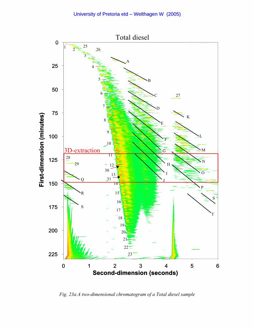
0
25
50
75
100
125
150
175
200
225
0 1 2 3 4 5 6Second-dimension (seconds)
Firs
t-dim
ensi
on (m
inut
es)
Total diesel262
3
4
5
6
7
8
A
27
9
10
11
12
13
14
15
16
17
18
1920
21
2223
30
31
2829
Q
R
S
T
B
C
D
E
F
G
H
IJ
K
L
M
N
O
P
251
S
3D-extraction
0
25
50
75
100
125
150
175
200
225
0 1 2 3 4 5 6Second-dimension (seconds)
Firs
t-dim
ensi
on (m
inut
es)
Total diesel262
3
4
5
6
7
8
A
27
9
10
11
12
13
14
15
16
17
18
1920
21
2223
30
31
2829
Q
R
S
T
B
C
D
E
F
G
H
IJ
K
L
M
N
O
P
251
S
3D-extraction
Fig. 23a A two-dimensional chromatogram of a Total diesel sample
UUnniivveerrssiittyy ooff PPrreettoorriiaa eettdd –– WWeelltthhaaggeenn WW ((22000055))
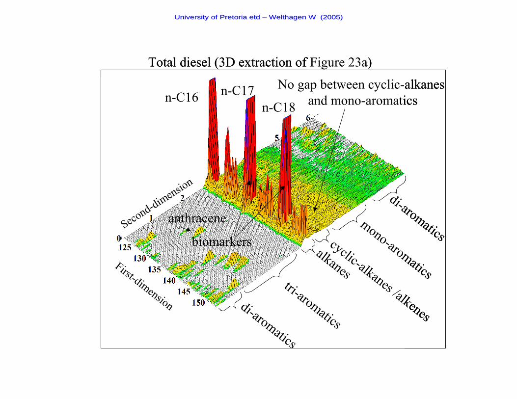
No gap between cyclic-alkanes and mono-aromatics
First-dimension
Second-dimension
n-C16 n-C17n-C18
alkanes
mono-aromatics
di-aromatics
tri-aromatics
anthracene
biomarkers cyclic-alkanes /alkenesdi-aromatics
Total diesel (3D extraction of Figure 23a)
No gap between cyclic-alkanes and mono-aromatics
First-dimension
Second-dimension
n-C16 n-C17n-C18
alkanes
mono-aromatics
di-aromatics
tri-aromatics
anthracene
biomarkers cyclic-alkanes /alkenesdi-aromatics
Total diesel (3D extraction of Figure 23a)
UUnniivveerrssiittyy ooff PPrreettoorriiaa eettdd –– WWeelltthhaaggeenn WW ((22000055))
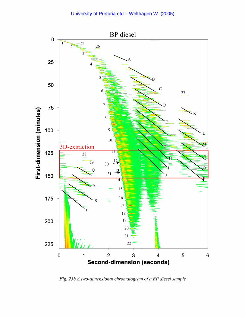
0
25
50
75
100
125
150
175
200
225
0 1 2 3 4 5 6Second-dimension (seconds)
Firs
t-dim
ensi
on (m
inut
es)
BP diesel262
3
4
5
6
7
8
A
27
9
10
11
12
13
14
15
16
17
18
19
20
21
22
30
31
28
29
Q
R
S
T
B
C
D
E
F
G
H
I
J
K
L
M
N
O
P
1 25
3D-extraction
0
25
50
75
100
125
150
175
200
225
0 1 2 3 4 5 6Second-dimension (seconds)
Firs
t-dim
ensi
on (m
inut
es)
BP diesel262
3
4
5
6
7
8
A
27
9
10
11
12
13
14
15
16
17
18
19
20
21
22
30
31
28
29
Q
R
S
T
B
C
D
E
F
G
H
I
J
K
L
M
N
O
P
1 25
3D-extraction
Fig. 23b A two-dimensional chromatogram of a BP diesel sample
UUnniivveerrssiittyy ooff PPrreettoorriiaa eettdd –– WWeelltthhaaggeenn WW ((22000055))
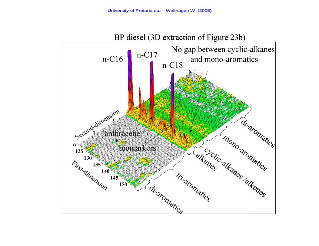
No gap between cyclic-alkanes and mono-aromatics
First-dimension
Second-dimension
n-C16 n-C17n-C18
alkanes
mono-aromatics
di-aromatics
tri-aromatics
anthracene
biomarkers cyclic-alkanes /alkenesdi-aromatics
BP diesel (3D extraction of Figure 23b)No gap between cyclic-alkanes
and mono-aromatics
First-dimension
Second-dimension
n-C16 n-C17n-C18
alkanes
mono-aromatics
di-aromatics
tri-aromatics
anthracene
biomarkers cyclic-alkanes /alkenesdi-aromatics
BP diesel (3D extraction of Figure 23b)
UUnniivveerrssiittyy ooff PPrreettoorriiaa eettdd –– WWeelltthhaaggeenn WW ((22000055))
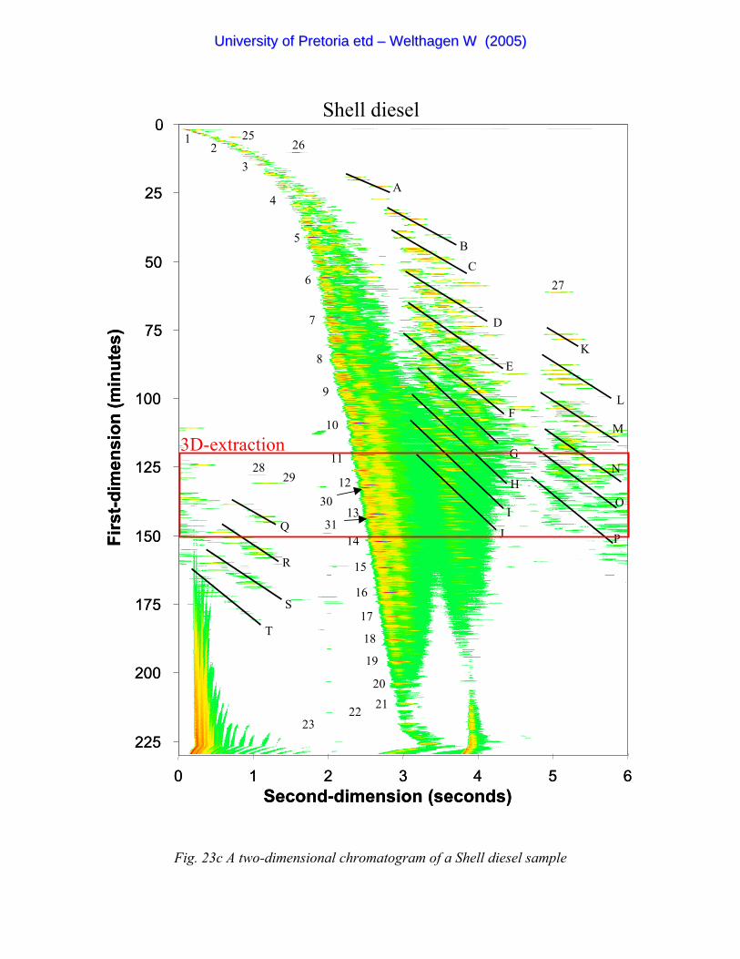
0
25
50
75
100
125
150
175
200
225
0 1 2 3 4 5 6Second-dimension (seconds)
Firs
t-dim
ensi
on (m
inut
es)
Shell diesel262
3
4
5
6
7
8
A
27
9
10
11
12
13
14
15
16
17
18
19
202122
23
30
31
2829
Q
R
S
T
BC
D
E
F
G
H
I
J
K
L
M
N
O
P
1 25
3D-extraction
0
25
50
75
100
125
150
175
200
225
0 1 2 3 4 5 6Second-dimension (seconds)
Firs
t-dim
ensi
on (m
inut
es)
Shell diesel262
3
4
5
6
7
8
A
27
9
10
11
12
13
14
15
16
17
18
19
202122
23
30
31
2829
Q
R
S
T
BC
D
E
F
G
H
I
J
K
L
M
N
O
P
1 25
3D-extraction
Fig. 23c A two-dimensional chromatogram of a Shell diesel sample
UUnniivveerrssiittyy ooff PPrreettoorriiaa eettdd –– WWeelltthhaaggeenn WW ((22000055))
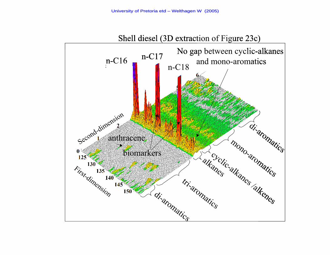
No gap between cyclic-alkanes and mono-aromatics
First-dimension
Second-dimension
n-C16 n-C17n-C18
alkanes
mono-aromatics
di-aromatics
tri-aromatics
anthracene
biomarkers cyclic-alkanes /alkenesdi-aromatics
Shell diesel (3D extraction of Figure 23c)No gap between cyclic-alkanes
and mono-aromatics
First-dimension
Second-dimension
n-C16 n-C17n-C18
alkanes
mono-aromatics
di-aromatics
tri-aromatics
anthracene
biomarkers cyclic-alkanes /alkenesdi-aromatics
Shell diesel (3D extraction of Figure 23c)
UUnniivveerrssiittyy ooff PPrreettoorriiaa eettdd –– WWeelltthhaaggeenn WW ((22000055))
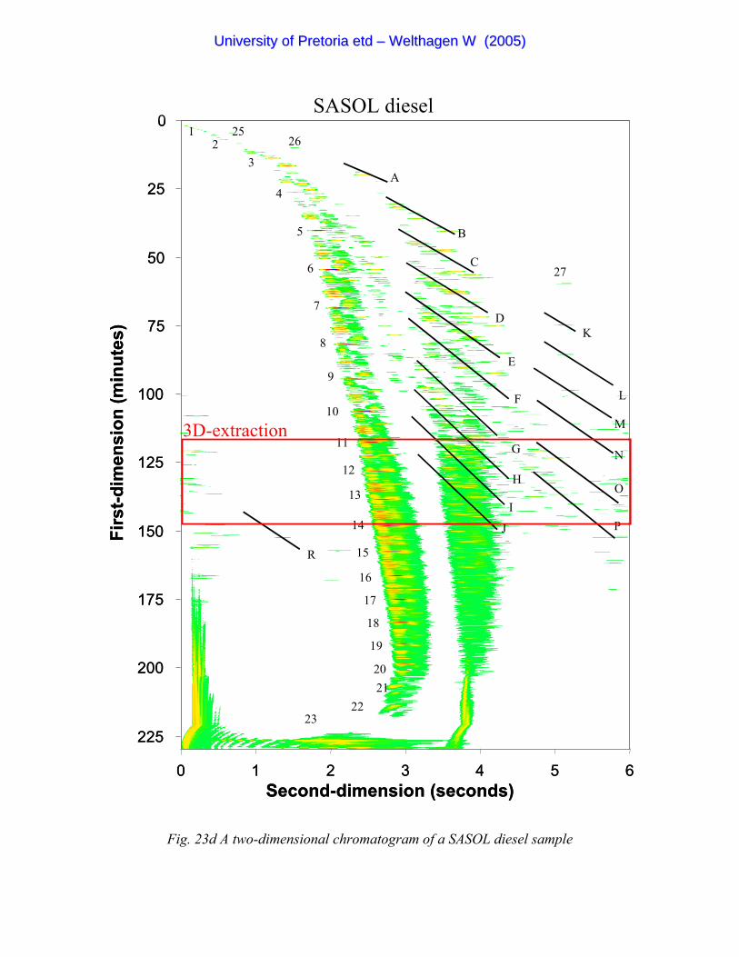
0
25
50
75
100
125
150
175
200
225
0 1 2 3 4 5 6Second-dimension (seconds)
Firs
t-dim
ensi
on (m
inut
es)
SASOL diesel262
3
4
5
6
7
8
A
27
9
10
11
12
13
14
15
16
17
18
19
2021
2223
R
B
C
D
E
F
G
H
I
J
K
L
M
N
O
P
1 25
3D-extraction
0
25
50
75
100
125
150
175
200
225
0 1 2 3 4 5 6Second-dimension (seconds)
Firs
t-dim
ensi
on (m
inut
es)
SASOL diesel262
3
4
5
6
7
8
A
27
9
10
11
12
13
14
15
16
17
18
19
2021
2223
R
B
C
D
E
F
G
H
I
J
K
L
M
N
O
P
1 25
3D-extraction
Fig. 23d A two-dimensional chromatogram of a SASOL diesel sample
UUnniivveerrssiittyy ooff PPrreettoorriiaa eettdd –– WWeelltthhaaggeenn WW ((22000055))
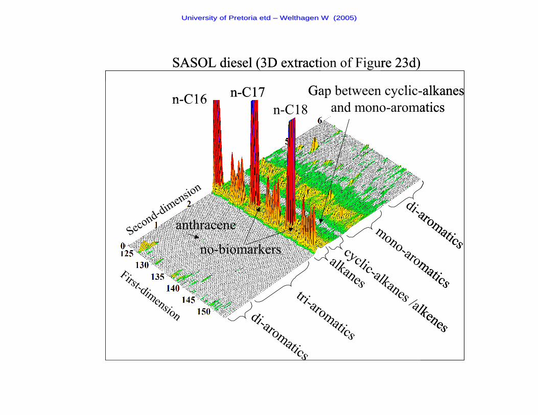
Gap between cyclic-alkanes and mono-aromatics
First-dimension
Second-dimension
n-C16 n-C17n-C18
alkanes
mono-aromatics
di-aromatics
tri-aromatics
anthracene
no-biomarkers cyclic-alkanes /alkenesdi-aromatics
SASOL diesel (3D extraction of Figure 23d)
Gap between cyclic-alkanes and mono-aromatics
First-dimension
Second-dimension
n-C16 n-C17n-C18
alkanes
mono-aromatics
di-aromatics
tri-aromatics
anthracene
no-biomarkers cyclic-alkanes /alkenesdi-aromatics
SASOL diesel (3D extraction of Figure 23d)
UUnniivveerrssiittyy ooff PPrreettoorriiaa eettdd –– WWeelltthhaaggeenn WW ((22000055))
-95-
The two-dimensional chromatograms of the four diesel samples can readily be differentiated. The
most obvious of these differences is in the group separations (aliphatic, mono-aromatic, di-aromatic
and tri-aromatic), the Total and Shell diesel shows almost no separation between the aliphatic and
mono-aromatic components while in the BP diesel there is a slight separation and in the SASOL
diesel baseline separation is observed. This is due to the relative concentrations of the cyclic-
alkanes (or alkenes) and the mono-aromatic compounds. Differences in case of individual
compounds are also found, this can be seen as peaks differing in colour in the respective
chromatograms. Another obvious difference is that the tri-aromatics (groups Q,R,S and T) and
biomarkers (peaks 30 and 31) in the SASOL diesel are almost absent. To be more specific on the
concentration variances software for quantitative analysis (peak integration) is required.
6.4 Analysis of diesel-paraffin mixtures
The use of these mixtures in the mining industry arises from their much cleaner exhaust emissions.
This is essential in a closed environment where the air needs to be circulated and remain safe for
human activity. These specially blended fuels for the mining vehicles perform exactly the same as
the diesels used on the surface but because of their lower aromatic content, their lubricating
properties are greatly reduced. In diesel engines the lubrication of the fuel is a very important factor
and can have a big influence on the lifespan and functionality of the engine.
As was seen in the previous section, a huge portion of the diesel constitutes aromatic compounds.
UUnniivveerrssiittyy ooff PPrreettoorriiaa eettdd –– WWeelltthhaaggeenn WW ((22000055))
-96-
In the Fischer-Tropsch diesel it was mentioned that there is a clear gap between the cyclic-alkanes
and the mono-aromatic part of the chromatogram, due to a lower concentration of the latter group.
The Fischer Tropsch process is known to produce diesel fractions of lower aromatic content. Low
aromatic content diesels provide less lubrication and are known to produce cleaner exhaust
emissions.
The same applies to the paraffin in that it has a high cetane number but almost no aromatics to
improve the lubrication. A further advantage of the paraffin is improved combustion of its shorter
alkane chain lengths, hence the cleaner exhaust gasses. To improve the lubricating properties of the
paraffin, aromatic compounds or a well lubricating diesel can be added. The study undertaken by
the Department of Mechanical Engineering at the University of Pretoria was focussed at determining
the fraction of diesel to give the optimal lubricating properties [56].
As the project of determining the best diesel-paraffin mixture was still in progress at the end of this
study, we can only speculate on the significance of our analytical results. Figure 24 shows the
different diesel-paraffin combinations evaluated. In the respective chromatograms, changes can be
seen in the alkane boiling point range (with the addition of diesel to the paraffin there are more
alkanes of higher mass). Also, as expected, the polar fraction of the paraffin increases with the
addition of diesel, to such an extend that, in the 66% diesel sample, even some tri-aromatics (group
Q the (CHx)1-anthracene and peak 29 anthracene) are observed. The mono-aromatics and di-
aromatics also increase with diesel concentration. In the pure paraffin sample, only the mono-
aromatics up to group G and di-aromatics up to group L can be observed. In the 66% paraffin
UUnniivveerrssiittyy ooff PPrreettoorriiaa eettdd –– WWeelltthhaaggeenn WW ((22000055))

-97-
mixture, group M of the di-aromatics appears and group I of the mono-aromatics appears in the 50%
paraffin sample. The 66% diesel mixture almost contains all the groups also observed in the pure
diesel sample apart from groups J and N. Interesting phenomena, like why the 66% paraffin mixture
has better lubricating properties than pure diesel, [56] cannot be explained at this stage.
UUnniivveerrssiittyy ooff PPrreettoorriiaa eettdd –– WWeelltthhaaggeenn WW ((22000055))
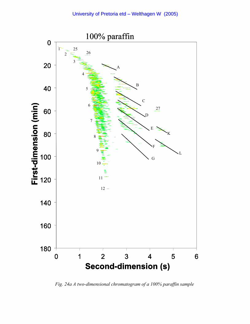
0
20
40
60
80
100
120
140
160
1800 1 2 3 4 5 6
Second-dimension (s)
Firs
t-dim
ensi
on (m
in)
25262
3
4
5
6
7
8
A
27
9
10
11
12
B
C
D
E
F
G
K
L
1
100% paraffin0
20
40
60
80
100
120
140
160
1800 1 2 3 4 5 6
Second-dimension (s)
Firs
t-dim
ensi
on (m
in)
0
20
40
60
80
100
120
140
160
1800 1 2 3 4 5 6
Second-dimension (s)
Firs
t-dim
ensi
on (m
in)
25262
3
4
5
6
7
8
A
27
9
10
11
12
B
C
D
E
F
G
K
L
1
100% paraffin
Fig. 24a A two-dimensional chromatogram of a 100% paraffin sample
UUnniivveerrssiittyy ooff PPrreettoorriiaa eettdd –– WWeelltthhaaggeenn WW ((22000055))
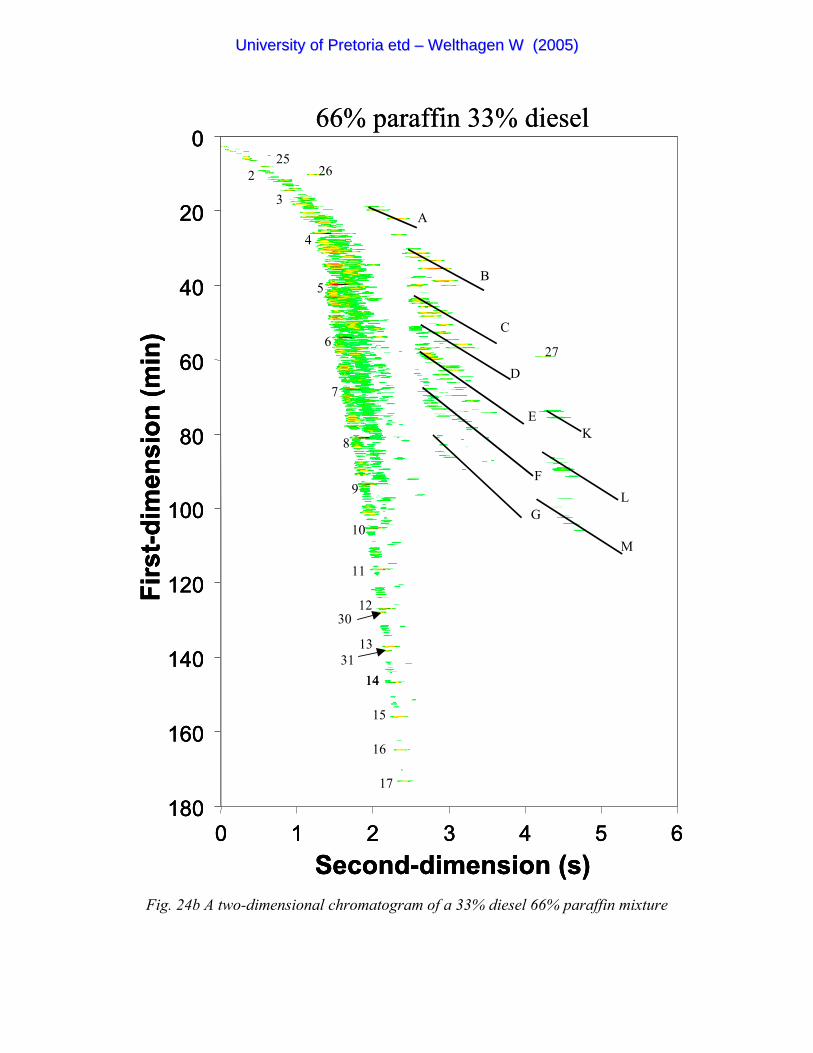
0
20
40
60
80
100
120
140
160
1800 1 2 3 4 5 6
Second-dimension (s)
Firs
t-dim
ensi
on (m
in)
25262
3
4
5
6
7
8
A
27
9
10
14
15
16
17
B
C
D
E
F
G
K
L
M
11
12
13
14
30
31
66% paraffin 33% diesel0
20
40
60
80
100
120
140
160
1800 1 2 3 4 5 6
Second-dimension (s)
Firs
t-dim
ensi
on (m
in)
0
20
40
60
80
100
120
140
160
1800 1 2 3 4 5 6
Second-dimension (s)
Firs
t-dim
ensi
on (m
in)
25262
3
4
5
6
7
8
A
27
9
10
14
15
16
17
B
C
D
E
F
G
K
L
M
11
12
13
14
30
31
66% paraffin 33% diesel
Fig. 24b A two-dimensional chromatogram of a 33% diesel 66% paraffin mixture
UUnniivveerrssiittyy ooff PPrreettoorriiaa eettdd –– WWeelltthhaaggeenn WW ((22000055))
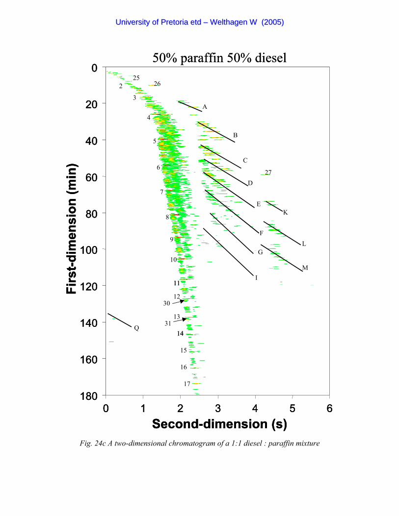
0
20
40
60
80
100
120
140
160
1800 1 2 3 4 5 6
Second-dimension (s)
Firs
t-dim
ensi
on (m
in)
25262
3
4
5
6
7
8
A
27
9
10
11
12
13
14
15
16
17
B
C
D
E
F
G
K
L
MI
11
14
30
31Q
50% paraffin 50% diesel0
20
40
60
80
100
120
140
160
1800 1 2 3 4 5 6
Second-dimension (s)
Firs
t-dim
ensi
on (m
in)
0
20
40
60
80
100
120
140
160
1800 1 2 3 4 5 6
Second-dimension (s)
Firs
t-dim
ensi
on (m
in)
25262
3
4
5
6
7
8
A
27
9
10
11
12
13
14
15
16
17
B
C
D
E
F
G
K
L
MI
11
14
30
31Q
50% paraffin 50% diesel
Fig. 24c A two-dimensional chromatogram of a 1:1 diesel : paraffin mixture
UUnniivveerrssiittyy ooff PPrreettoorriiaa eettdd –– WWeelltthhaaggeenn WW ((22000055))
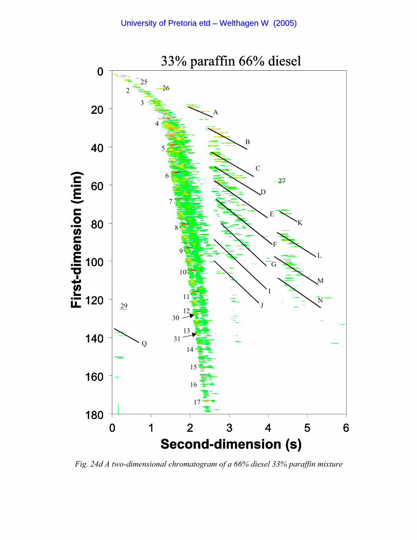
0
20
40
60
80
100
120
140
160
1800 1 2 3 4 5 6
Second-dimension (s)
Firs
t-dim
ensi
on (m
in)
25262
3
4
5
6
7
8
A
27
9
10
11
12
13
14
15
16
17
30
31
29
B
C
D
E
F
G
K
L
MI
NJ
Q
33% paraffin 66% diesel0
20
40
60
80
100
120
140
160
1800 1 2 3 4 5 6
Second-dimension (s)
Firs
t-dim
ensi
on (m
in)
0
20
40
60
80
100
120
140
160
1800 1 2 3 4 5 6
Second-dimension (s)
Firs
t-dim
ensi
on (m
in)
25262
3
4
5
6
7
8
A
27
9
10
11
12
13
14
15
16
17
30
31
29
B
C
D
E
F
G
K
L
MI
NJ
Q
33% paraffin 66% diesel
Fig. 24d A two-dimensional chromatogram of a 66% diesel 33% paraffin mixture
UUnniivveerrssiittyy ooff PPrreettoorriiaa eettdd –– WWeelltthhaaggeenn WW ((22000055))
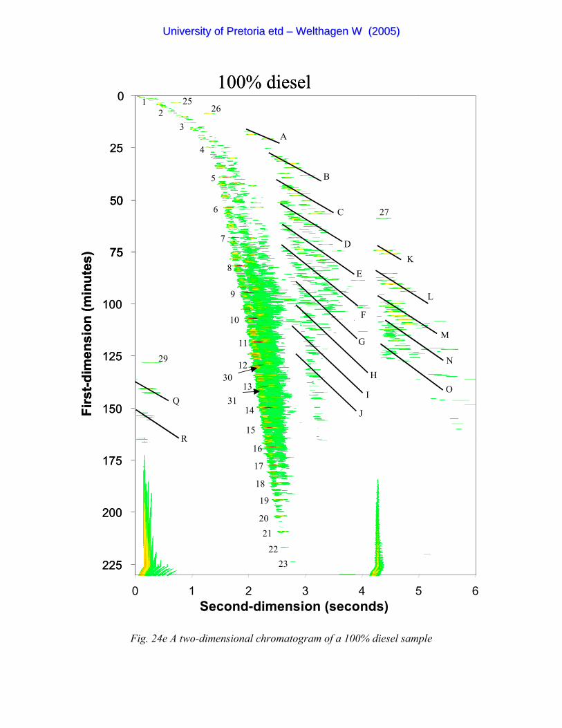
0
25
50
75
100
125
150
175
200
225
0 1 2 3 4 5 6Second-dimension (seconds)
Firs
t-dim
ensi
on (m
inut
es)
50
75
25262
3
4
5
6
7
8
A
27
1
9
10
11
12
13
14
15
16
17
18
19
2021
2223
30
31
29
Q
R
B
C
D
E
F
G
H
I
J
K
L
M
N
O
100% diesel0
25
50
75
100
125
150
175
200
225
0 1 2 3 4 5 6Second-dimension (seconds)
Firs
t-dim
ensi
on (m
inut
es)
50
75
25262
3
4
5
6
7
8
A
27
1
9
10
11
12
13
14
15
16
17
18
19
2021
2223
30
31
29
Q
R
B
C
D
E
F
G
H
I
J
K
L
M
N
O
100% diesel
Fig. 24e A two-dimensional chromatogram of a 100% diesel sample
UUnniivveerrssiittyy ooff PPrreettoorriiaa eettdd –– WWeelltthhaaggeenn WW ((22000055))
-103-
Chapter 7
Conclusion
Table of Contents
7.1 Optimisation of GC x GC
7.2 The analysis of diesel petrochemical samples
UUnniivveerrssiittyy ooff PPrreettoorriiaa eettdd –– WWeelltthhaaggeenn WW ((22000055))
-104-
Chapter 7
Conclusion
In this dissertation the goal was to provide a guideline for the optimisation of GC x GC, as such a
process is a lot more complex than in normal gas chromatography. The path taken to achieve this
optimisation led to some interesting and previously ignored parameters that play an integral role in
GC x GC performance. These included the careless use of “rules of thumb” to optimise linear
flow rates, and the blind use of calculations done by the instrumentation without knowing the margin
of error or even the formulas used!
It was also shown that GC x GC can be applied very successfully to the analysis of complex
mixtures such as diesel petroleum samples. The applications on the diesel samples range from
fingerprinting to quantitative component analysis.
7.1 Optimisation of GC x GC
The optimisation of a comprehensively coupled system proved to be a very complex procedure.
Frequently used “rules of thumb” for the optimisation of one-dimensional systems involve
approximations that are not obvious without careful understanding of the original optimisation
studies. The one common error is to use the generally specified linear flow rate for a given column
UUnniivveerrssiittyy ooff PPrreettoorriiaa eettdd –– WWeelltthhaaggeenn WW ((22000055))
-105-
inner diameter and the type of carrier gas. The optimum linear flow rate specified for columns with
different diameters is good under conventional, atmospheric pressure conditions but is based on
carrier gas diffusitivities at atmospheric pressures, that do not apply directly to high pressure exit
conditions. In GC x GC such high pressures exist since the second dimension acts as a restrictor at
the end of the first column and diffusion in the carrier gas slows down appreciably. This change
in the diffusion can be clearly seen in the calculations done to determine the optimum linear flow
rates. The van Deemter optimum flow rate for hydrogen in a 0.25 mm internal diameter column is
in the order of 40 to 50 cm/s, but we determined that our system has a optimum linear flow rate in
its first dimension of 30 to 35 cm/s which corresponds almost to the optimum linear flow rate of
helium under normal pressure conditions in a similar column. As a synergistic effect, the lower
values of the first-dimension linear flow rate also result in much improved second-dimension
resolution due to the lower linear flow rates and a yet unknown modulator effect.
When the second-dimension Van Deemter plot was drawn, some interesting results were obtained.
It has to be reminded that a Van Deemter plot of this dimension is reasonable since it is run under
isothermal conditions. The last part of the curve usually dictated by the Cu-term was a lot steeper
than plots of similar column dimensions. This is believed to be the result of a less than perfect
modulator that gives a measurable contribution to the second-dimension bandwidth.
The simplified flow optimisation method is justified and is recommended for any similar
optimisation studies where different columns need to be coupled in GC x GC (verified for test
compounds with second-dimension retention factors larger than three (k > 3)). The final suggested
UUnniivveerrssiittyy ooff PPrreettoorriiaa eettdd –– WWeelltthhaaggeenn WW ((22000055))
-106-
inlet pressure (110 kPa) which is slightly too low for the first-dimensions and sightly too high for
the second gives extremely improved results to the chromatogram (Figure 18) where a “rule of
thumb” linear flow rate (of 50 cm/s) is used. The use of a wide boiling point range test sample such
as diesel seems justified, as the modulator optimisation is strongly dependent on column oven
temperatures and therefore needs to be checked over a wide temperature range.
In summary we propose an overall GC x GC optimisation guideline that involves the following
steps:
1 Column selection (first- and second-dimension column length, internal diameter and film
thickness) and carrier gas selection.
2 Stationary phase selection (based on dimensionality considerations, the polarity range of the
compounds within the sample and thermal stability of the column phases)
3 Temperature programming of the first-dimension and modulation period chosen to maintain
the recommended four second-dimension analyses per first-dimension peak. These
parameters would depend on the type of analysis and consideration of the speed vs resolution
trade-off.
4 Versification of modulator performance over the full column temperature range anticipated
for the sample.
5 Flow optimisation (resolution calculations of selected test compounds at different system
inlet pressures). This is required once a new set of column dimensions is selected, that has
not previously been optimised with the selected carrier gas. Test compounds should be well
retained in both dimensions (k >3). A new set of column dimensions should be selected, if
UUnniivveerrssiittyy ooff PPrreettoorriiaa eettdd –– WWeelltthhaaggeenn WW ((22000055))
-107-
the first- and the second-dimension linear flow optima are not compatible.
5 Second-dimension offset temperature should finally be adjusted so that the polarity range
of the sample utilizes the full space of the two-dimensional separation plane without any
“wrap-around”
7.2 The analysis of diesel petrochemical samples
This study confirmed the recent literature reports that GC x GC is a powerful technique for the
analysis of petrochemical samples. In this method development study, different diesel samples were
analysed and in their respective one-dimensional plots, clear differences can be seen regarding, for
example, n-alkane patterns. These differences, however, are not clear enough to speculate on the
differences in the total composition of the samples with different lubrication and combustion
properties . In one-dimensional analysis, too many compounds co-elute and many are thus not
identifiable. When involving two-dimensional separations, these smaller differences can be
investigated. Under visual inspection differences can be easily spotted, which is a clear indication
that this method can be used for fingerprinting purposes.
UUnniivveerrssiittyy ooff PPrreettoorriiaa eettdd –– WWeelltthhaaggeenn WW ((22000055))
-108-
References
1 Giddings, J.C., 1984, Analytical Chemistry, vol. 56, p. 1258A
2 Giddings, J.C., 1967, Analytical Chemistry, vol. 39, p. 1927
3 Guiochon, G., Beaver, L.A., Gonnord, M.F., Siouffi, A.M., Zakaria, M.J., 1983, Journal of
Chromatographia, vol. 255, p. 415
4 Liu, Z., Phillips, J.B., 1991, Journal of Chromatographic Science, vol. 29, p. 227-231
5 Blomberg, J., Schoenmakers, P.J., Brinkman, U.A.Th.,2002, Journal of Chromatography A,
vol. 972, p. 137
6 Marriott, P.J., Kinghorn, R.M. 2000, Journal of Chromatographia, vol. 866, p. 203
7 Beens, J., Blomberg, J., Boelens, H., Tijssen, R., 1998, Journal of High Resolution
Chromatography, vol. 21, p. 47
8 Phillips, J.B, 1995. Jounal of Chromatograpic Science, vol. 33, p. 55
9 Burger B.V., Snyman, T., Burger W.J.G., van Rooyen, W.F., 2003, Journal of Separation
UUnniivveerrssiittyy ooff PPrreettoorriiaa eettdd –– WWeelltthhaaggeenn WW ((22000055))
-109-
Science, vol. 26, p. 123
10 Marriott, P.J., Kinghorn, R.M., 1997, Analytical Chemistry, vol. 69, p. 2582
11 Ledford, E. B., Billesbach, C., 2000, Journal of High Resolution Chromatography, vol. 23,
p. 202
12 Ledford, E.B., Billesbach, C.A., Zhu, Q.Y., 2000, Journal of High Resolution
Chromatography, vol. 23, p. 205
13 Beens, J., Adahchour, M., Vreuls, R.J.J., van Altena, K., Brinkman, U.ATh, 2001, Jurnal of
Chromatography, vol. 919, p. 127
14 Bruckner, C.A., Prazen, C.A., Synovec, R.E., 1998, Analytical Chemistry, vol. 70, p. 2796
15 Beens. J., 2002, School in comprehensive two-dimensional gas chromatography at the 25th
International Symposium on Capillary Chromatography, 13-17 May 2002, Rive del Garda,
Italy
16 Beens, J., Blomberg, J., Tijssen, R., 1998, Journal of chromatography, vol. 882, p. 233
17 http://www.leco.com/mass-spectrometers/peg/gcxgc/diesel.pdf 23 January 2003
UUnniivveerrssiittyy ooff PPrreettoorriiaa eettdd –– WWeelltthhaaggeenn WW ((22000055))
-110-
18 Davis, J.M., Giddings, J.C., 1983, Analytical Chemistry, vol. 55, p. 418
19 Davis, J.M., Giddings, J.C., 1985, Analytical Chemistry, vol. 57, p. 2168
20 Phillips, J.B., Beens, J., 1999, Journal of Chromatography, vol. 856, p. 331
21 Giddings, J.C., 1995, Journal of Chromatography, vol. 703, p. 3
22 Poole, C.F., Poole, S.K., 1991 Chromatography Today, Elsevier, Amsterdam, The
Netherlands
23 Skoog, D.A., Holler, F.J., Nieman, T.A., 1998, Principles of instrumental analysis. Fifth
edition, Saunders College Publishing, Philadelphia, USA.
24 Restek corp. Chromatographic Products Catalogue 2002
25 Persinger, H.E., Shank, J.T., 1974, Journal of Chromatography Science, vol. 11, p. 190
26 Cramers, C.A., Jansen, H.G., van Deursen, M.M., Leclercq, P.A., 1999, Journal of
Chromatography A, vol. 856, p. 315
27 Schomburg, G., 1990, Gas Chromatography a Practical Course, VCH Weinheim New York
UUnniivveerrssiittyy ooff PPrreettoorriiaa eettdd –– WWeelltthhaaggeenn WW ((22000055))
-111-
28 Desty, D.H., Goldup, A., Swanton, W.T., Gas Chromatography, Brenner, N. et al (Eds.),
Academic Press, New York, USA, 1962, p. 105
29 Knox, J.H., Saleem, M., 1969, Journal of Chromatographic Science, vol. 7, p. 614
30 Giddings, J.C., 1962, Analytical Chemistry, vol. 34, p. 314
31 Sandra, P., 1989, Journal of High Resolution Chromatography, vol. 12, p. 273
32 Korytar, P., Jansen, H.G., Brinkman, U.A.Th., Matisovaa, E., 2002, TrAC Trends in
analytical chemistry, vol. 21, p. 558
33 Ong, R., Marriott, P., Morrison, P., Haglund, P., 2002, Journal of Chromatography, vol. 962,
p. 135
33 Martin, A.J.P., 1958, Desty, D.H.(ED), Gas Chromatography, Butterworths, London, UK
34 Schwartz, R.D., Mathews, R.G., Daderic, G., Brasseaux, D.J., 1967, Journal of Gas
Chromatography, vol. 5, p. 251
35 Rijks, J.A., Cramers, C.A., 1974, Chromatographia, vol. 7, p. 99
UUnniivveerrssiittyy ooff PPrreettoorriiaa eettdd –– WWeelltthhaaggeenn WW ((22000055))
-112-
36 Grob, K., Voellmin, J.A., 1969, Beitrieb Tabakforsching, vol. 5, p. 52
37 Grob, K.,1973, Chemical Industry, London, vol. 6, p. 248
38 Dandeneau, R.D., Zerenner, E.H., 1979, Journal of High Resolution Chromatography, vol.
6, p. 351
39 Luke, L., Ray, J.E., 1985, Journal of High Resolution Chromatography, vol. 8, p. 193
40 Trestianu, S., Zilioli, G., Sironi, A., Saravalle, C., Munari, F., Galli, M., Gaspar,G., Colin,
J.M., Jovelin,J.L., 1985, Journal of High Resolution Chromatography, vol. 8, p. 93
41 Boer, H., van Arkel, P., 1971, Chromatographia, vol. 4, p. 300
42 Boer, H., van Arkel, P., Boersma, W.J., 1980, Chromatographia, vol. 13, p. 500
43 Brown, R.A., Taylor, R.C., Melpolder, F.W., Young, W.S.,1948, Analytical Chemistry, vol.
20, p. 5
43 Holmes, J.C., Morrell, F.A., 1957, Applied Spectroscopy, vol. 11, p. 86
44 Marriott, P.J., Kinghorn, R.M. 2000, Chromatographia, vol.866, p. 203
UUnniivveerrssiittyy ooff PPrreettoorriiaa eettdd –– WWeelltthhaaggeenn WW ((22000055))
-113-
46 Beens, J., Blomberg, J., Boelens, H., Tijssen, R., 1998, Journal of High Resolution
Chromatography, vol. 21, p. 47
47 Frysinger, G.S., Gaines, R.B.,2000, Proc. 23rd International Symposium on Capillary
Chromatography, Riva del Garda, Italy, 5-9 June 2000, I.O.P.M.S., Kortrijk, Belgium
48 Van Deursen, M., Beens, J., Blomberg, J., Reijenga, J., Lipman, P., Cramers, C., 2000,
Journal of High Resolution Chromatography, vol.23, p.507
49 Zellelow, A.Z., 2003, Dissertation on the analysis of essential oils with GC x GC.,
University of Pretoria, South Africa.
50 Gaines, R.B., Ledford Jr, E.B., Stuart, J.D., 1998, Journal of Microcolumn Separation, vol.
10, p. 597
51 Gaines, R.B., Frysinger, G.S., Hendrick-Smith, M.S., Stuart, J.D., 1999, Environmental
Science Technology, vol. 33, p. 2106
52 Golay, M.J.E., 1958, Gas Chromatography, (Hrsg.) D.H. Desty Butterworth, London, p. 36
53 Van Deemter, I.J., Zuiderweg, F.J., Klinkenberg, A., 1956, Chemical Engineering Science,
vol. 5, p. 271
UUnniivveerrssiittyy ooff PPrreettoorriiaa eettdd –– WWeelltthhaaggeenn WW ((22000055))
-114-
54 Frysinger, G.S., Gaines, R.B., Ledford Jr, E.B., 1999, Journal of High Resolution
Chromatgraphy, vol. 22, p. 195
55 Blomberg, J., Multidimensional GC-based separations for the oil and petrochemical industry.
Thesis for the degree of doctor, Vrije Universiteit Amsterdam, The Netherlands, 2002
56 Oppermann, T. Department of Mechanical Engineering at the University of Pretoria,
Personal communications, 2003
UUnniivveerrssiittyy ooff PPrreettoorriiaa eettdd –– WWeelltthhaaggeenn WW ((22000055))
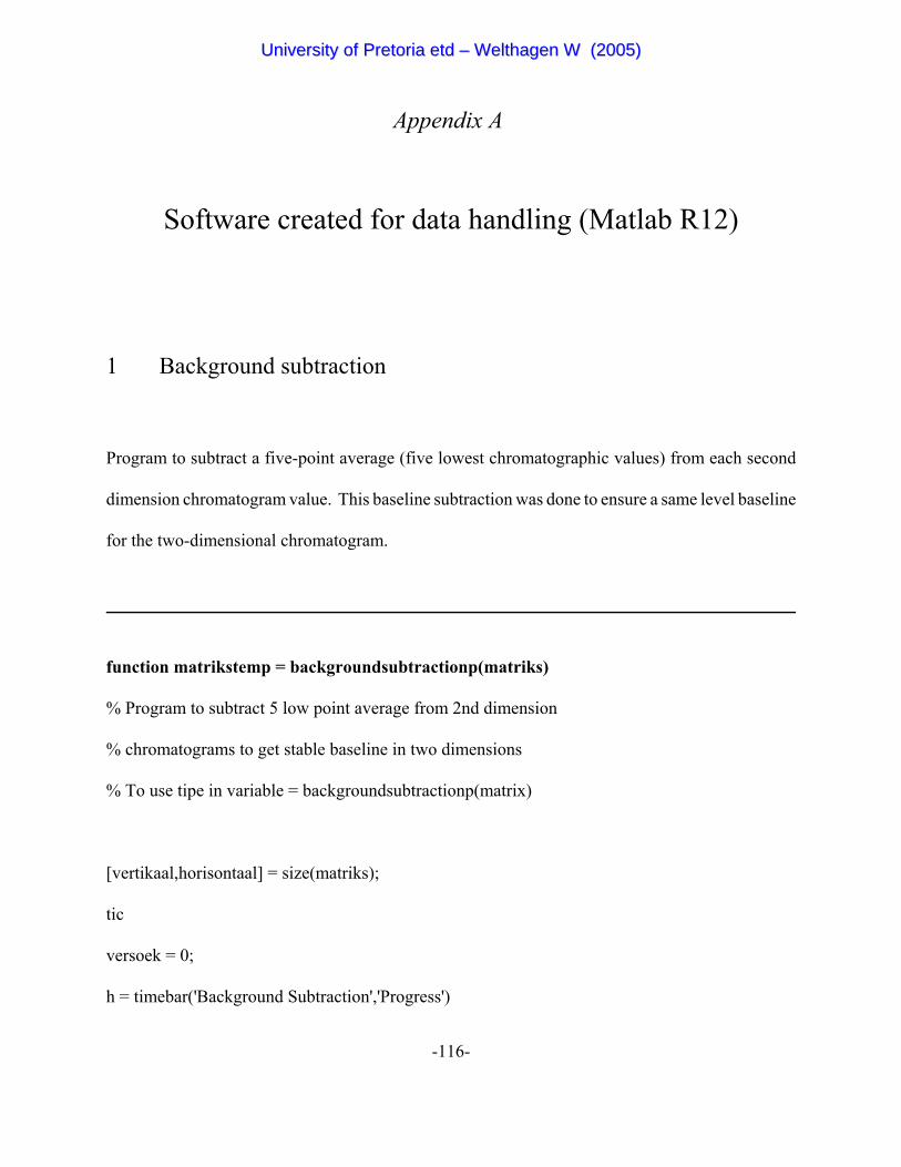
-116-
Appendix A
Software created for data handling (Matlab R12)
1 Background subtraction
Program to subtract a five-point average (five lowest chromatographic values) from each second
dimension chromatogram value. This baseline subtraction was done to ensure a same level baseline
for the two-dimensional chromatogram.
function matrikstemp = backgroundsubtractionp(matriks)
% Program to subtract 5 low point average from 2nd dimension
% chromatograms to get stable baseline in two dimensions
% To use tipe in variable = backgroundsubtractionp(matrix)
[vertikaal,horisontaal] = size(matriks);
tic
versoek = 0;
h = timebar('Background Subtraction','Progress')
UUnniivveerrssiittyy ooff PPrreettoorriiaa eettdd –– WWeelltthhaaggeenn WW ((22000055))
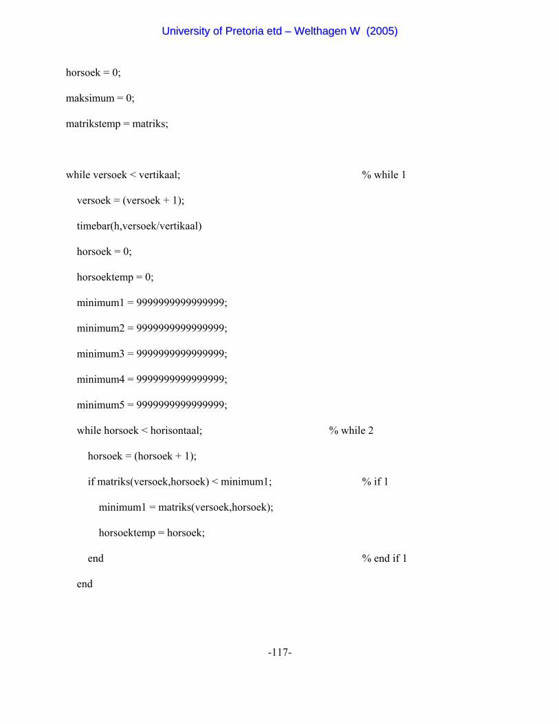
-117-
horsoek = 0;
maksimum = 0;
matrikstemp = matriks;
while versoek < vertikaal; % while 1
versoek = (versoek + 1);
timebar(h,versoek/vertikaal)
horsoek = 0;
horsoektemp = 0;
minimum1 = 9999999999999999;
minimum2 = 9999999999999999;
minimum3 = 9999999999999999;
minimum4 = 9999999999999999;
minimum5 = 9999999999999999;
while horsoek < horisontaal; % while 2
horsoek = (horsoek + 1);
if matriks(versoek,horsoek) < minimum1; % if 1
minimum1 = matriks(versoek,horsoek);
horsoektemp = horsoek;
end % end if 1
end
UUnniivveerrssiittyy ooff PPrreettoorriiaa eettdd –– WWeelltthhaaggeenn WW ((22000055))
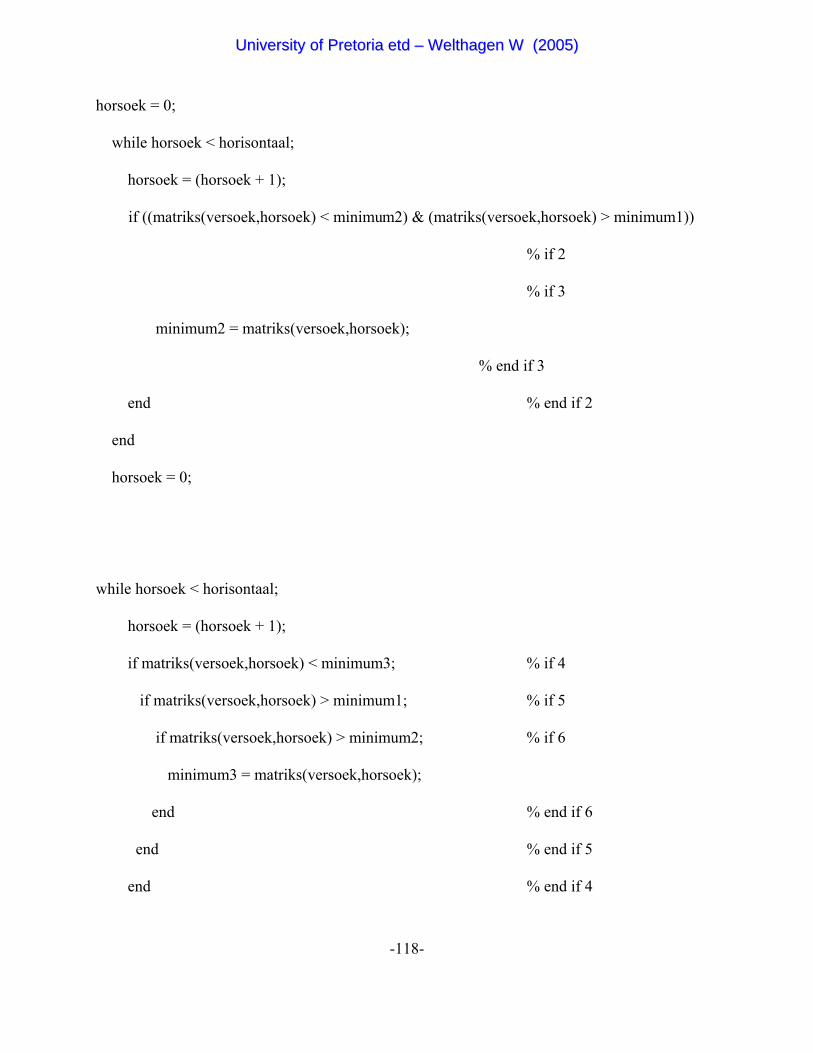
-118-
horsoek = 0;
while horsoek < horisontaal;
horsoek = (horsoek + 1);
if ((matriks(versoek,horsoek) < minimum2) & (matriks(versoek,horsoek) > minimum1))
% if 2
% if 3
minimum2 = matriks(versoek,horsoek);
% end if 3
end % end if 2
end
horsoek = 0;
while horsoek < horisontaal;
horsoek = (horsoek + 1);
if matriks(versoek,horsoek) < minimum3; % if 4
if matriks(versoek,horsoek) > minimum1; % if 5
if matriks(versoek,horsoek) > minimum2; % if 6
minimum3 = matriks(versoek,horsoek);
end % end if 6
end % end if 5
end % end if 4
UUnniivveerrssiittyy ooff PPrreettoorriiaa eettdd –– WWeelltthhaaggeenn WW ((22000055))
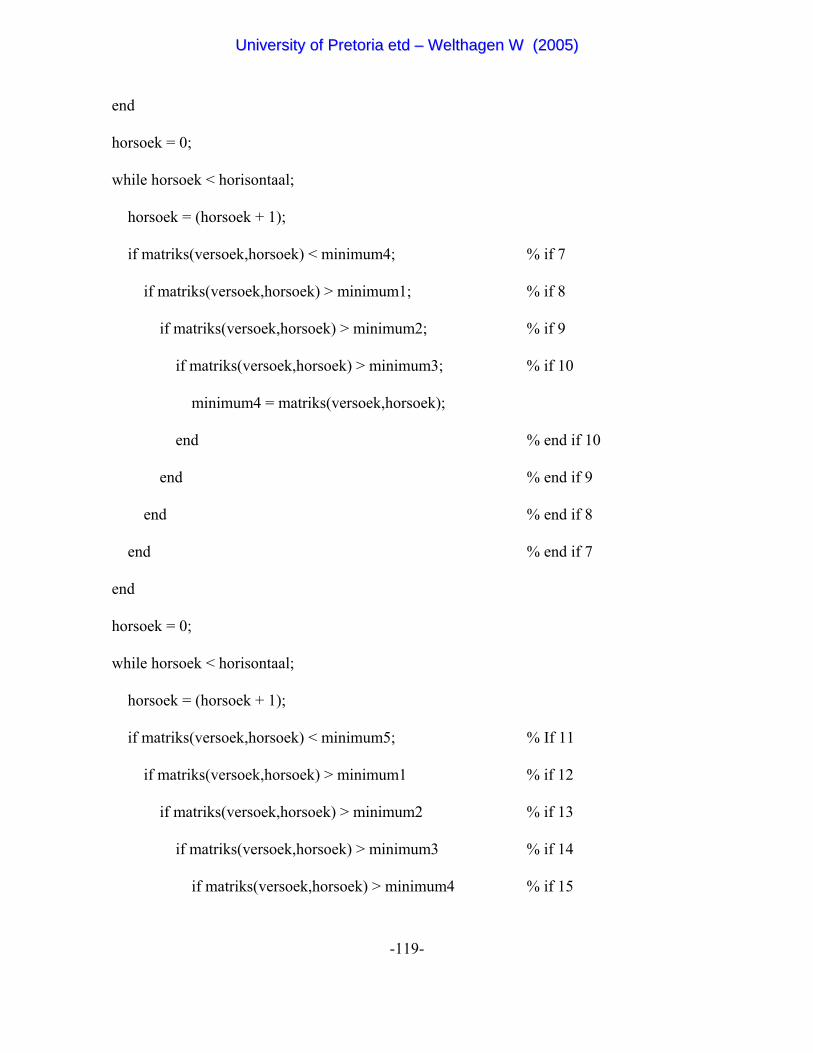
-119-
end
horsoek = 0;
while horsoek < horisontaal;
horsoek = (horsoek + 1);
if matriks(versoek,horsoek) < minimum4; % if 7
if matriks(versoek,horsoek) > minimum1; % if 8
if matriks(versoek,horsoek) > minimum2; % if 9
if matriks(versoek,horsoek) > minimum3; % if 10
minimum4 = matriks(versoek,horsoek);
end % end if 10
end % end if 9
end % end if 8
end % end if 7
end
horsoek = 0;
while horsoek < horisontaal;
horsoek = (horsoek + 1);
if matriks(versoek,horsoek) < minimum5; % If 11
if matriks(versoek,horsoek) > minimum1 % if 12
if matriks(versoek,horsoek) > minimum2 % if 13
if matriks(versoek,horsoek) > minimum3 % if 14
if matriks(versoek,horsoek) > minimum4 % if 15
UUnniivveerrssiittyy ooff PPrreettoorriiaa eettdd –– WWeelltthhaaggeenn WW ((22000055))
-120-
minimum5 = matriks(versoek,horsoek);
end % end if 15
end % end if 14
end % end if 13
end % end if 12
end % end if 11
end
% end while 2
t = [minimum1 minimum2 minimum3 minimum4 minimum5];
gemideld = ((minimum1 + minimum2 + minimum3 + minimum4 + minimum5) / 5);
count1 = 0;
for count1 = 1 : horisontaal
matrikstemp(versoek,count1) = matrikstemp(versoek,count1) - gemideld;
end
end % end while 1
close(h)
matrikstemp;
matriks;
toc
UUnniivveerrssiittyy ooff PPrreettoorriiaa eettdd –– WWeelltthhaaggeenn WW ((22000055))
-121-
2 Program to reconstruct the one-dimensional chromatogram
Program for the reconstructing of a one dimensional chromatogram from a two-dimensional array
by adding up all the values of any given second-dimension chromatogram, analogous to the
reconstructed total ion chromatogram from GC-MS raw data
function onedimensionchrom(matriks)
% drawing one dimensional chromatogram from a dwo dimensional data set
[vertikaal,horisontaal] = size(matriks);
matrikstemp = matriks';
teller = 1:vertikaal;
i = 99999999;
while i > 99999
i = input('What is the modulation period of the chromatogram in seconds ?: ');
if i > 99999
iii = input('The modulation period must be an interger between 0 and 99999 seconds !!! ');
end
end
naam = input('What is the name of your chromatogram ?','s');
tottyd = (vertikaal*i)/60;
tydinkrement = tottyd/10;
UUnniivveerrssiittyy ooff PPrreettoorriiaa eettdd –– WWeelltthhaaggeenn WW ((22000055))
-122-
onechrom=sum(matrikstemp(1:end,teller));
plot(onechrom)
inkrement = vertikaal/10;
set(gca,'XTick',inkrement:inkrement:vertikaal)
set(gca,'XTickLabel',{tydinkrement:tydinkrement:tottyd}),xlabel('minutes')
ylabel('intensity')
title(['1 Dimensional Plot of ',naam])
UUnniivveerrssiittyy ooff PPrreettoorriiaa eettdd –– WWeelltthhaaggeenn WW ((22000055))
-123-
3 Program to extract individual second-dimension chromatograms
This program was designed to extract individual second-dimension chromatograms from the two-
dimensional data array and plot it in a one-dimensional chromatogram.
function matrikstwee = twodimensionchrom(matriks)
% drawing two dimensional chromatogram from a one dimensional data set
[vertikaal,horisontaal] = size(matriks);
matrikstemp = matriks';
teller = 1:(vertikaal-1);
i = 99999999;
t = 99999999;
col = 99999999;
while i > 99999
i = input('What is the modulation period of the chromatogram in seconds ?: ');
if i > 99999
iii = input('The modulation period must be an interger between 0 and 99999 seconds !!! ');
end
end
while t > 99999
t = input('What is the sampling rate in Hz ?: ');
UUnniivveerrssiittyy ooff PPrreettoorriiaa eettdd –– WWeelltthhaaggeenn WW ((22000055))
-124-
if t > 99999
ttt = input('The sampling rate must be between 0 and 99999 Hz !!! ');
end
end
while col > 99999
col = input('What is the column you whish to plot -- amu = column + 1 + minmass exported ---:
');
if col > 99999
colll = input('The column must be between 0 and 99999 !!! ');
end
end
inkrement = i * t
aantalchroms = vertikaal/inkrement
herstel = round(aantalchroms)
tydelik = matriks([1:inkrement], col);
teller = 0;
while teller < (herstel - 1);
teller = (teller + 1);
volg = inkrement;
volg = (volg * teller);
UUnniivveerrssiittyy ooff PPrreettoorriiaa eettdd –– WWeelltthhaaggeenn WW ((22000055))
-125-
h = (volg + 1);
n = (volg + inkrement);
tydelik2 = matriks([h:n], col);
tydelik = [tydelik tydelik2];
end
matrikstwee = tydelik';
UUnniivveerrssiittyy ooff PPrreettoorriiaa eettdd –– WWeelltthhaaggeenn WW ((22000055))
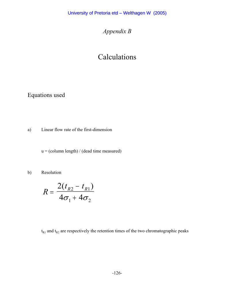
-126-
Appendix B
Calculations
Equations used
a) Linear flow rate of the first-dimension
u = (column length) / (dead time measured)
b) Resolution
Rt tR R=
−+
24 4
2 1
1 2
( )σ σ
tR1 and tR2 are respectively the retention times of the two chromatographic peaks
UUnniivveerrssiittyy ooff PPrreettoorriiaa eettdd –– WWeelltthhaaggeenn WW ((22000055))
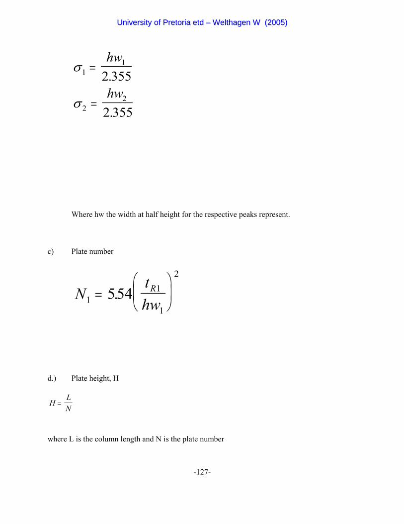
-127-
σ
σ
11
22
2 355
2 355
=
=
hw
hw.
.
Where hw the width at half height for the respective peaks represent.
c) Plate number
Nthw
R1
1
1
2
554=⎛⎝⎜
⎞⎠⎟.
d.) Plate height, H
HLN
=
where L is the column length and N is the plate number
UUnniivveerrssiittyy ooff PPrreettoorriiaa eettdd –– WWeelltthhaaggeenn WW ((22000055))
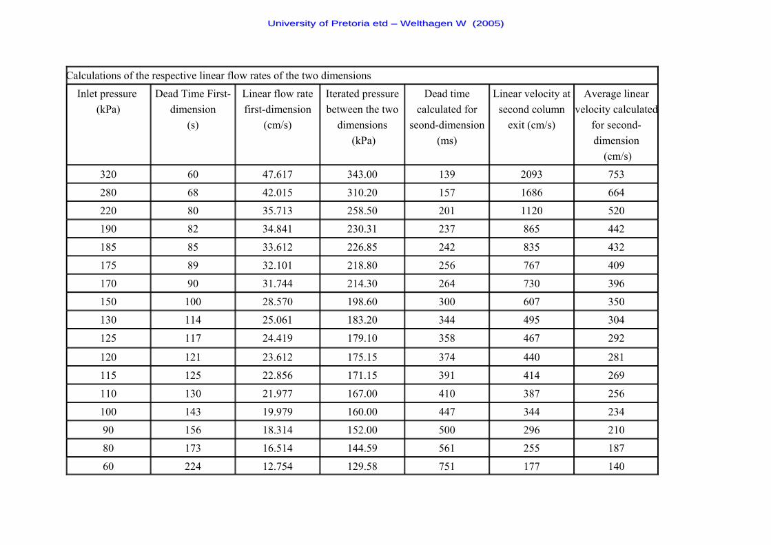
Calculations of the respective linear flow rates of the two dimensions
Inlet pressure (kPa)
Dead Time First-dimension
(s)
Linear flow ratefirst-dimension
(cm/s)
Iterated pressurebetween the two
dimensions (kPa)
Dead timecalculated for
seond-dimension(ms)
Linear velocity atsecond column
exit (cm/s)
Average linearvelocity calculated
for second-dimension
(cm/s)
320 60 47.617 343.00 139 2093 753
280 68 42.015 310.20 157 1686 664
220 80 35.713 258.50 201 1120 520
190 82 34.841 230.31 237 865 442
185 85 33.612 226.85 242 835 432
175 89 32.101 218.80 256 767 409
170 90 31.744 214.30 264 730 396
150 100 28.570 198.60 300 607 350
130 114 25.061 183.20 344 495 304
125 117 24.419 179.10 358 467 292
120 121 23.612 175.15 374 440 281
115 125 22.856 171.15 391 414 269
110 130 21.977 167.00 410 387 256
100 143 19.979 160.00 447 344 234
90 156 18.314 152.00 500 296 210
80 173 16.514 144.59 561 255 187
60 224 12.754 129.58 751 177 140
UUnniivveerrssiittyy ooff PPrreettoorriiaa eettdd –– WWeelltthhaaggeenn WW ((22000055))
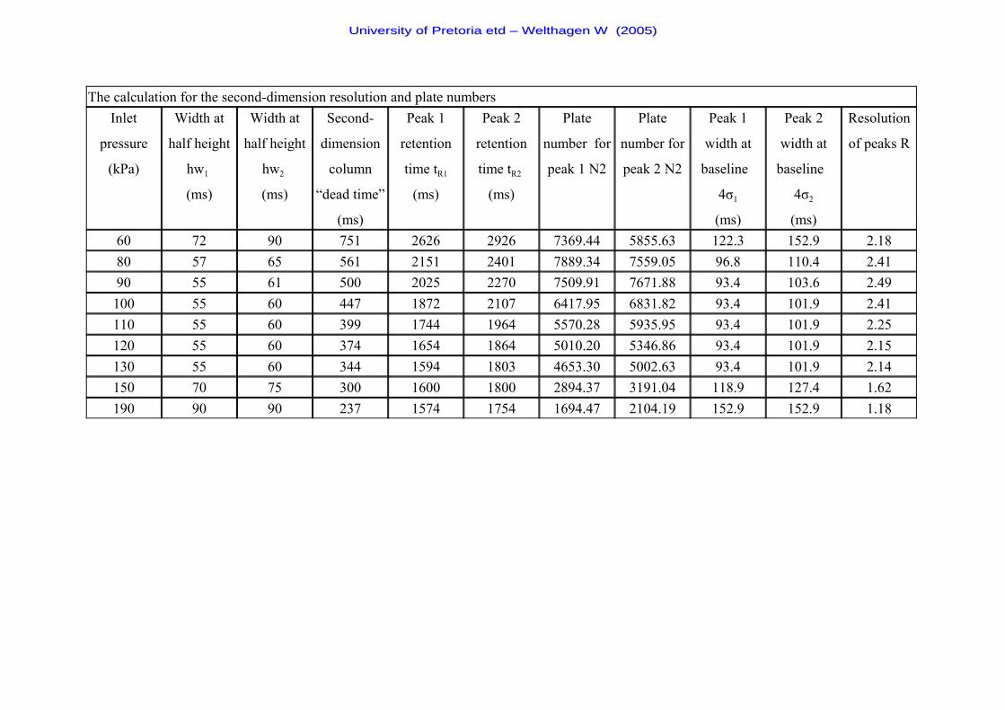
The calculation for the second-dimension resolution and plate numbersInlet
pressure
(kPa)
Width at
half height
hw1
(ms)
Width at
half height
hw2
(ms)
Second-
dimension
column
“dead time”
(ms)
Peak 1
retention
time tR1
(ms)
Peak 2
retention
time tR2
(ms)
Plate
number for
peak 1 N2
Plate
number for
peak 2 N2
Peak 1
width at
baseline
4σ1
(ms)
Peak 2
width at
baseline
4σ2
(ms)
Resolution
of peaks R
60 72 90 751 2626 2926 7369.44 5855.63 122.3 152.9 2.1880 57 65 561 2151 2401 7889.34 7559.05 96.8 110.4 2.4190 55 61 500 2025 2270 7509.91 7671.88 93.4 103.6 2.49100 55 60 447 1872 2107 6417.95 6831.82 93.4 101.9 2.41110 55 60 399 1744 1964 5570.28 5935.95 93.4 101.9 2.25120 55 60 374 1654 1864 5010.20 5346.86 93.4 101.9 2.15130 55 60 344 1594 1803 4653.30 5002.63 93.4 101.9 2.14150 70 75 300 1600 1800 2894.37 3191.04 118.9 127.4 1.62190 90 90 237 1574 1754 1694.47 2104.19 152.9 152.9 1.18
UUnniivveerrssiittyy ooff PPrreettoorriiaa eettdd –– WWeelltthhaaggeenn WW ((22000055))
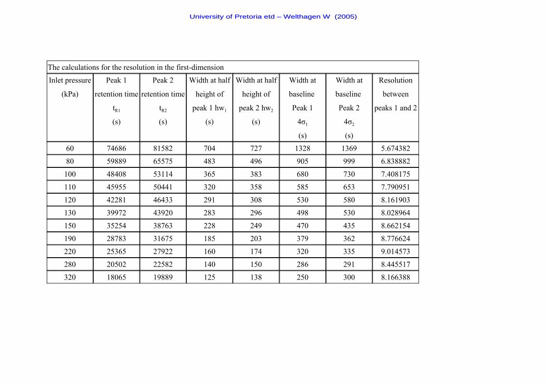
The calculations for the resolution in the first-dimension
Inlet pressure
(kPa)
Peak 1
retention time
tR1
(s)
Peak 2
retention time
tR2
(s)
Width at half
height of
peak 1 hw1
(s)
Width at half
height of
peak 2 hw2
(s)
Width at
baseline
Peak 1
4σ1
(s)
Width at
baseline
Peak 2
4σ2
(s)
Resolution
between
peaks 1 and 2
60 74686 81582 704 727 1328 1369 5.674382
80 59889 65575 483 496 905 999 6.838882
100 48408 53114 365 383 680 730 7.408175
110 45955 50441 320 358 585 653 7.790951
120 42281 46433 291 308 530 580 8.161903
130 39972 43920 283 296 498 530 8.028964
150 35254 38763 228 249 470 435 8.662154
190 28783 31675 185 203 379 362 8.776624
220 25365 27922 160 174 320 335 9.014573
280 20502 22582 140 150 286 291 8.445517
320 18065 19889 125 138 250 300 8.166388
UUnniivveerrssiittyy ooff PPrreettoorriiaa eettdd –– WWeelltthhaaggeenn WW ((22000055))
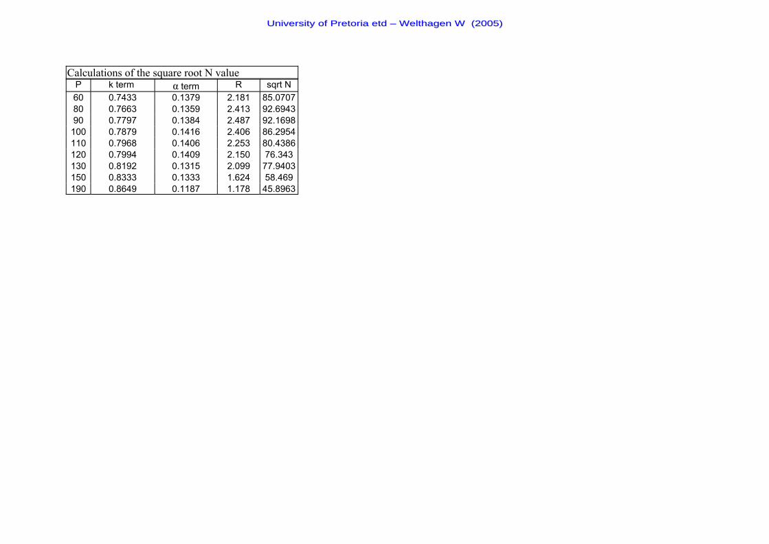
Calculations of the square root N valueP k term α term R sqrt N60 0.7433 0.1379 2.181 85.070780 0.7663 0.1359 2.413 92.694390 0.7797 0.1384 2.487 92.1698100 0.7879 0.1416 2.406 86.2954110 0.7968 0.1406 2.253 80.4386120 0.7994 0.1409 2.150 76.343130 0.8192 0.1315 2.099 77.9403150 0.8333 0.1333 1.624 58.469190 0.8649 0.1187 1.178 45.8963
UUnniivveerrssiittyy ooff PPrreettoorriiaa eettdd –– WWeelltthhaaggeenn WW ((22000055))