The Optical Flow Field

Caltech, Oct. 2004

Lihi Zelnik-Manor

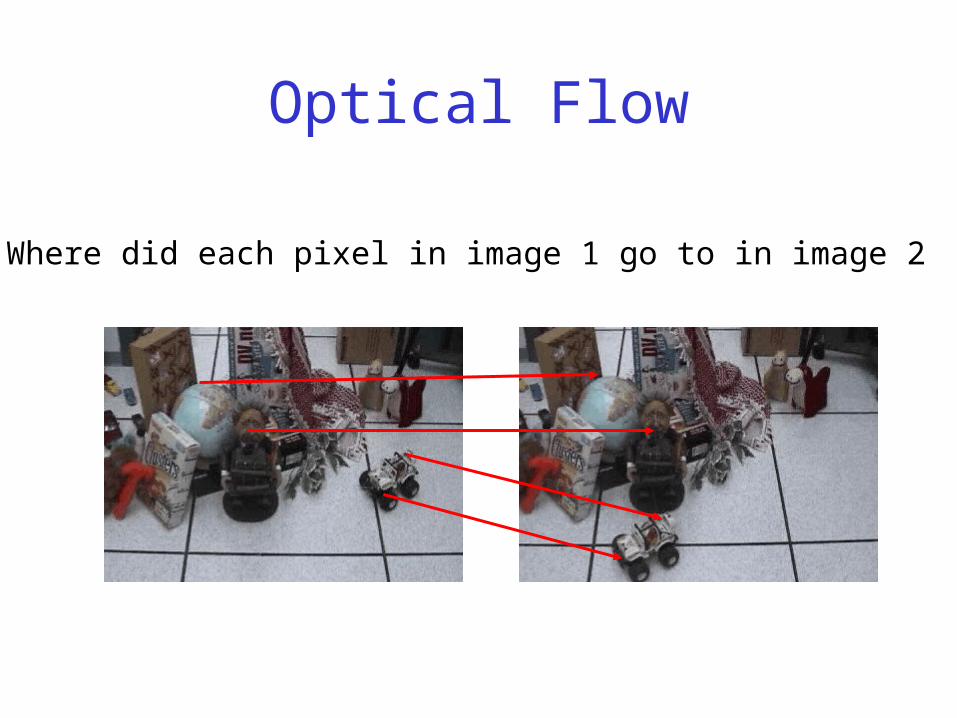
Optical Flow

Where did each pixel in image 1 go to in image 2

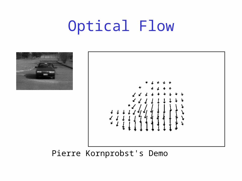
Optical Flow

Pierre Kornprobst's Demo

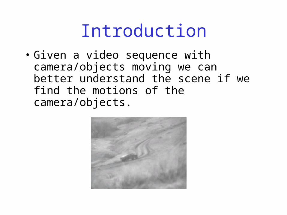
Introduction• Given a video sequence with

camera/objects moving we can better understand the scene if we find the motions of the camera/objects.

Scene Interpretation

• How is the camera moving?• How many moving objects are there?• Which directions are they moving in?• How fast are they moving?• Can we recognize their type of motion (e.g.

walking, running, etc.)?

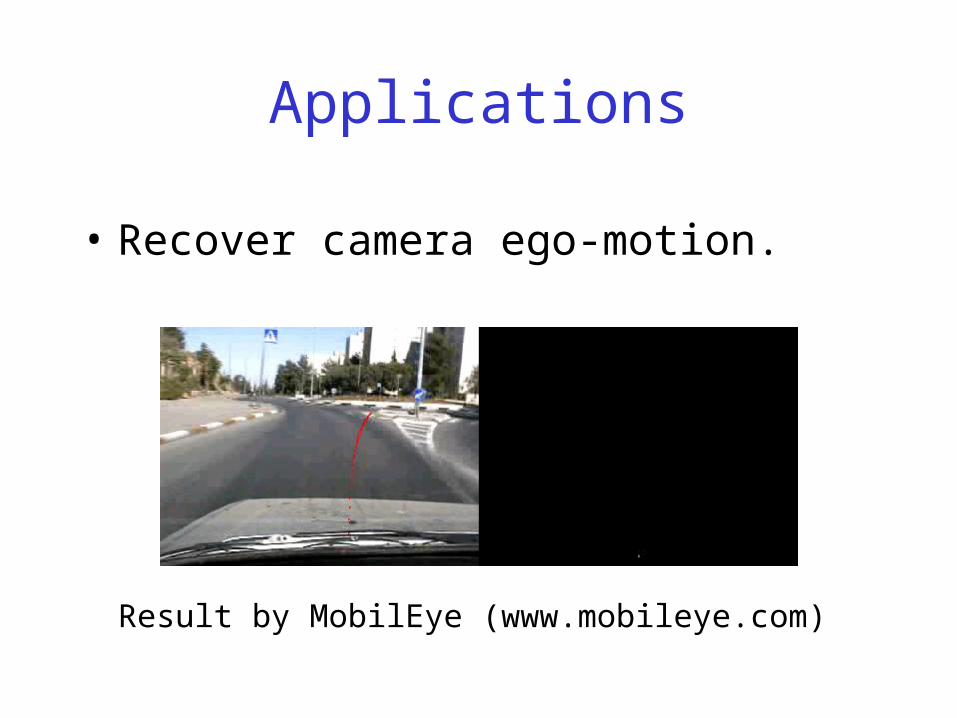
Applications

• Recover camera ego-motion.

Result by MobilEye (www.mobileye.com)

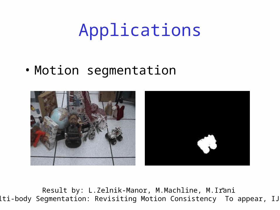
Applications

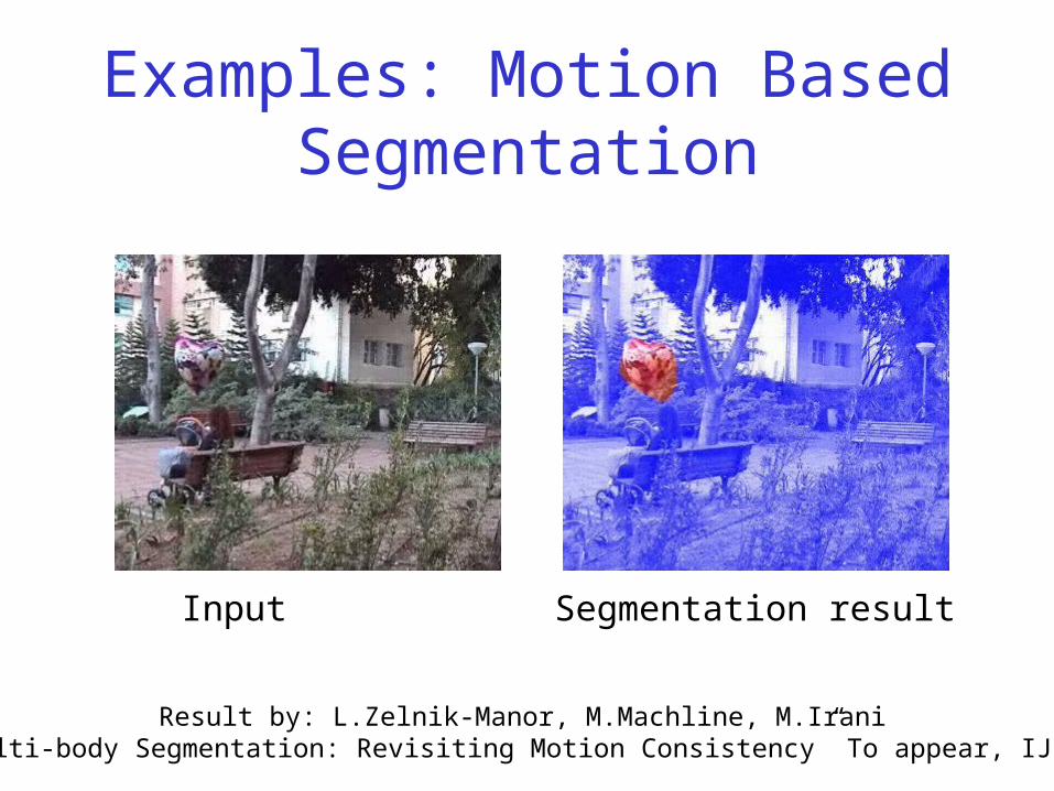
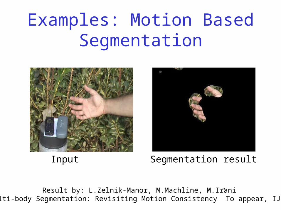
• Motion segmentation

Result by: L.Zelnik-Manor, M.Machline, M.Irani“Multi-body Segmentation: Revisiting Motion Consistency” To appear, IJCV

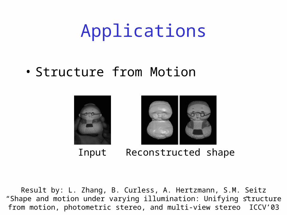
Applications

• Structure from Motion

Input Reconstructed shape

Result by: L. Zhang, B. Curless, A. Hertzmann, S.M. Seitz“Shape and motion under varying illumination: Unifying structure from motion, photometric

stereo, and multi-view stereo” ICCV’03

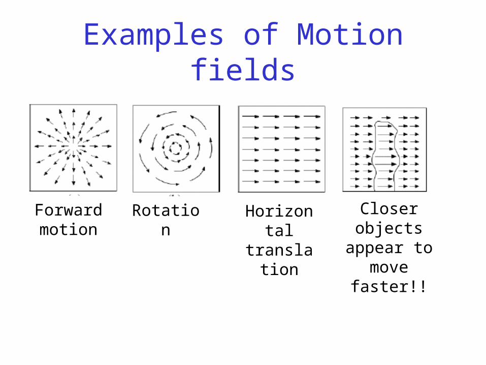
Examples of Motion fields

Forward motion

Rotation Horizontal translation

Closer objects

appear to move faster!!

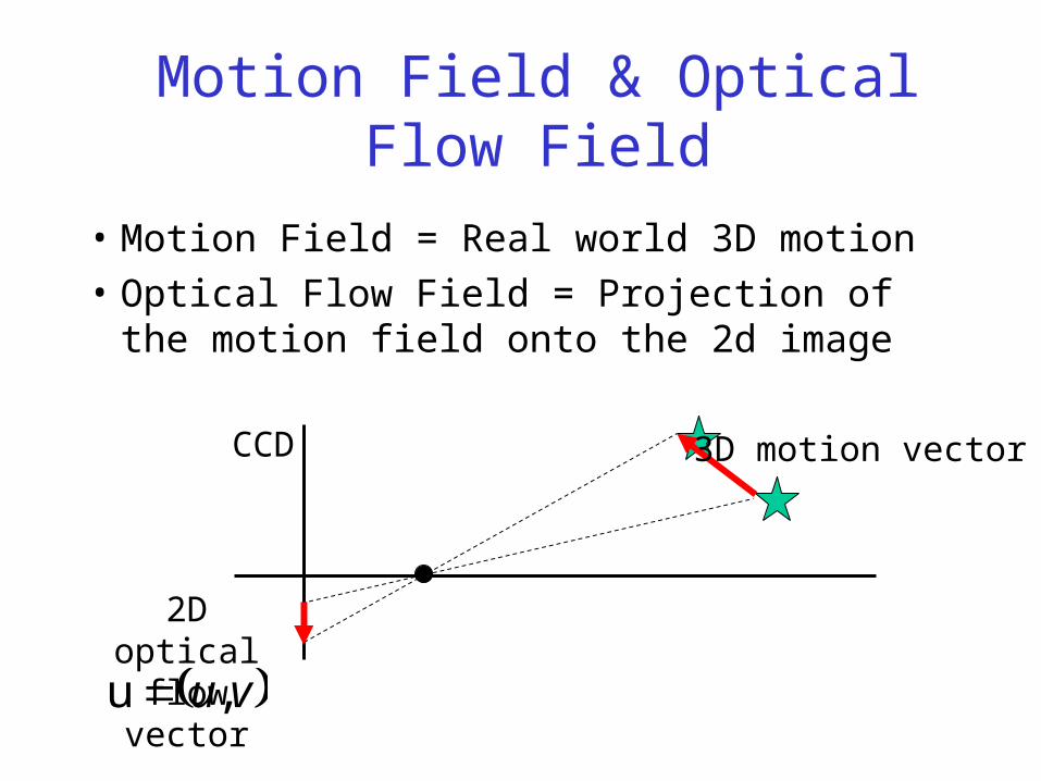
Motion Field & Optical Flow Field

• Motion Field = Real world 3D motion

• Optical Flow Field = Projection of the motion field onto the 2d image

3D motion vector

2D optical flow vector

vu,u

CCD

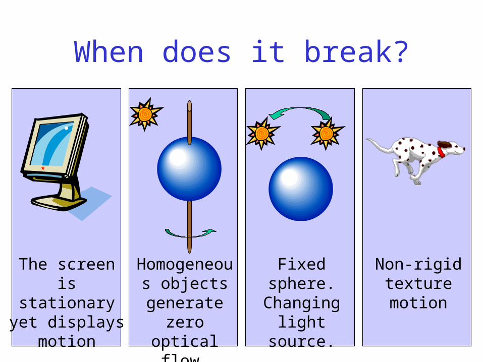
When does it break?

The screen is stationary yet

displays motion

Homogeneous objects

generate zero optical flow.

Fixed sphere. Changing light

source.

Non-rigid texture motion

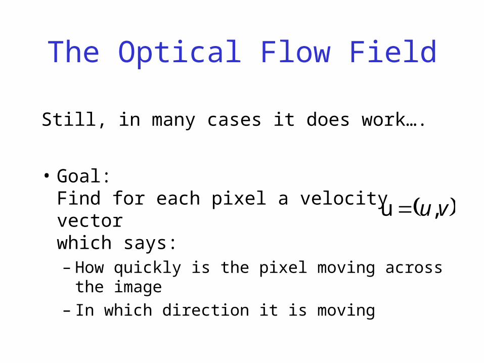
The Optical Flow Field

Still, in many cases it does work….

• Goal:Find for each pixel a velocity vector which says:– How quickly is the pixel moving across the image– In which direction it is moving

vu,u

How do we actually do that?

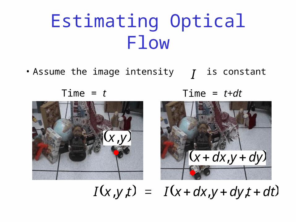
Estimating Optical Flow

• Assume the image intensity is constant

tyxI ,, dttdyydxxI ,,

ITime = t Time = t+dt

dyydxx ,

yx,

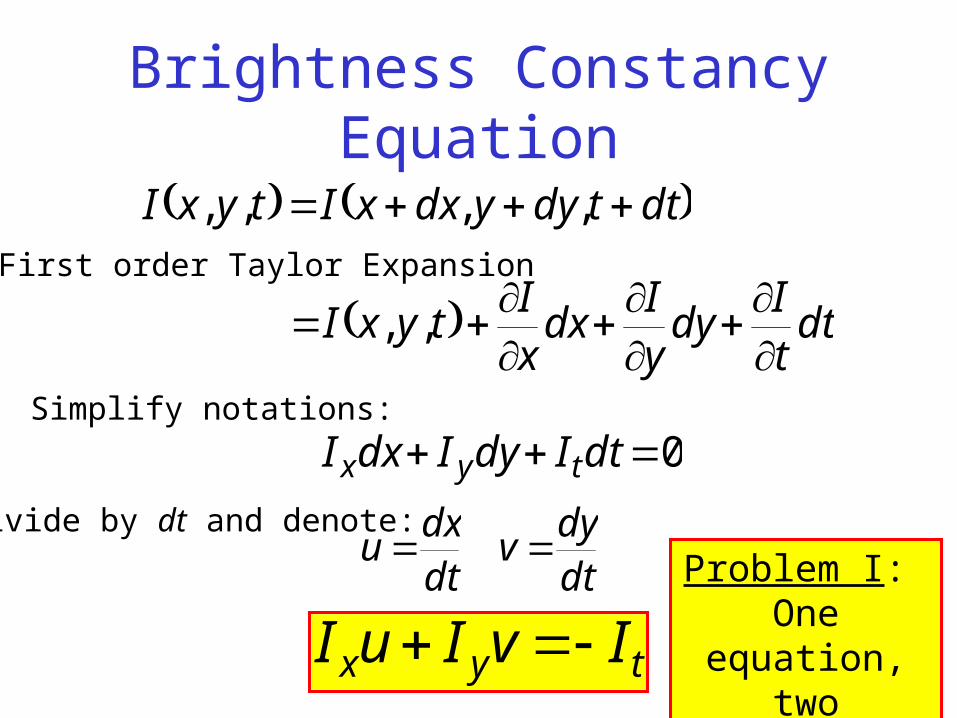
Brightness Constancy Equation

dttdyydxxItyxI ,,,,

dttI

dyyI

dxxI

tyxI

,,

First order Taylor Expansion

0 dtIdyIdxI tyx

Simplify notations:

Divide by dt and denote:

dtdx

u dtdy

v

tyx IvIuI Problem I: One equation, two

unknowns

Time t+dt

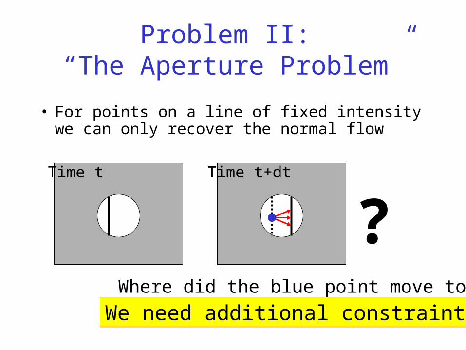
Problem II: “The Aperture Problem”

Time t

?Time t+dt

Where did the blue point move to?

We need additional constraints

• For points on a line of fixed intensity we can only recover the normal flow

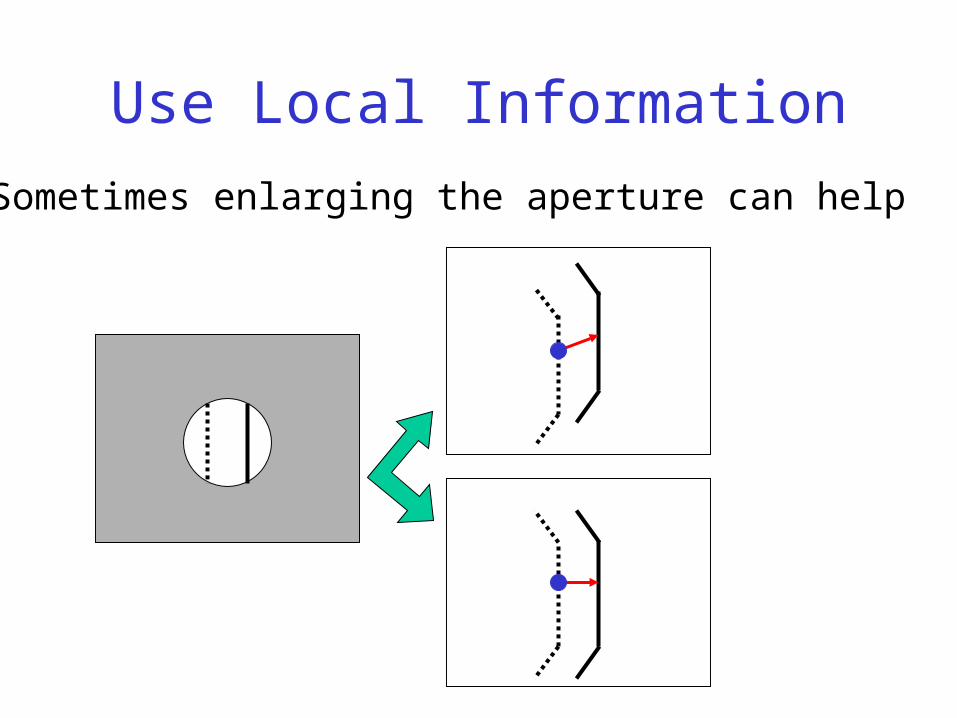
Use Local Information

Sometimes enlarging the aperture can help

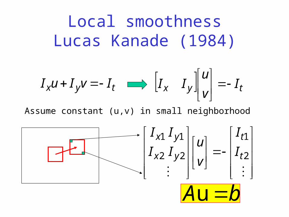
Local smoothnessLucas Kanade (1984)

Assume constant (u,v) in small neighborhood

tyx IvIuI tyx Iv

uII

2

1

22

11

t

t

yx

yx

I

I

v

uII

II

bA u

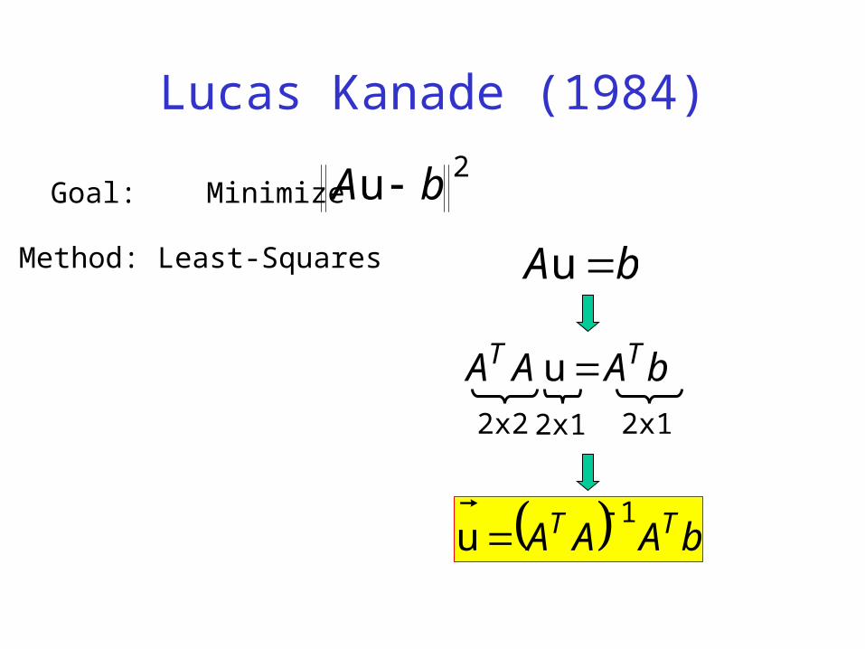
Lucas Kanade (1984)

bA u

bAAA TT 1u

Goal: Minimize2u bA

bAAA TT u

2x2 2x1 2x1

Method: Least-Squares

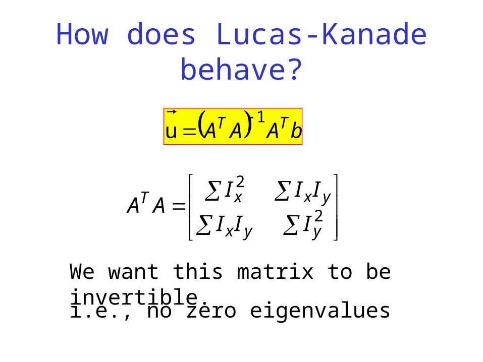
How does Lucas-Kanade behave?

2

2

yyx

yxxT

III

IIIAA

We want this matrix to be invertible.

i.e., no zero eigenvalues

bAAA TT 1u

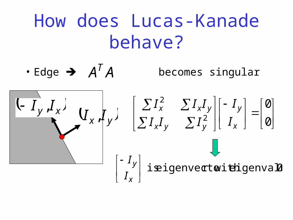
How does Lucas-Kanade behave?

• Edge becomes singularAAT

yx II , xy II ,

0

02

2

x

y

yyx

yxx

I

I

III

III

0 eigenvaluer with eigenvecto is

x

y

I

I

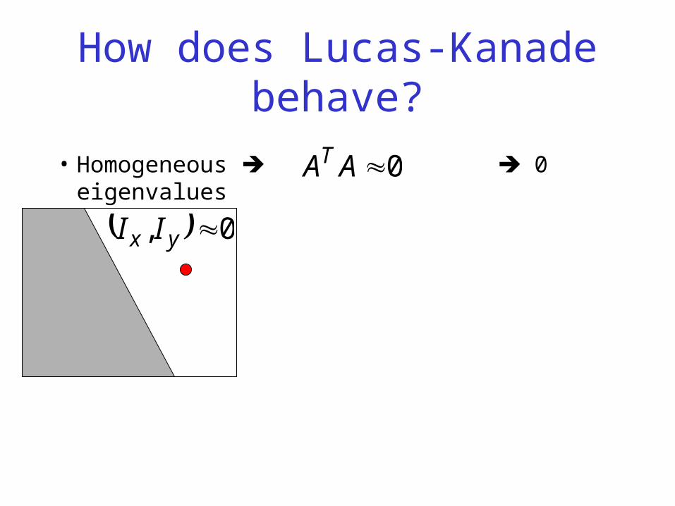
How does Lucas-Kanade behave?

• Homogeneous 0 eigenvalues0AAT

0, yx II

How does Lucas-Kanade behave?

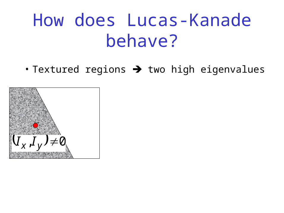
• Textured regions two high eigenvalues

0, yx II

How does Lucas-Kanade behave?

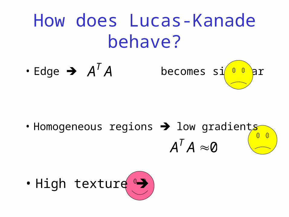
• Edge becomes singular

0AAT

AAT

• Homogeneous regions low gradients

• High texture

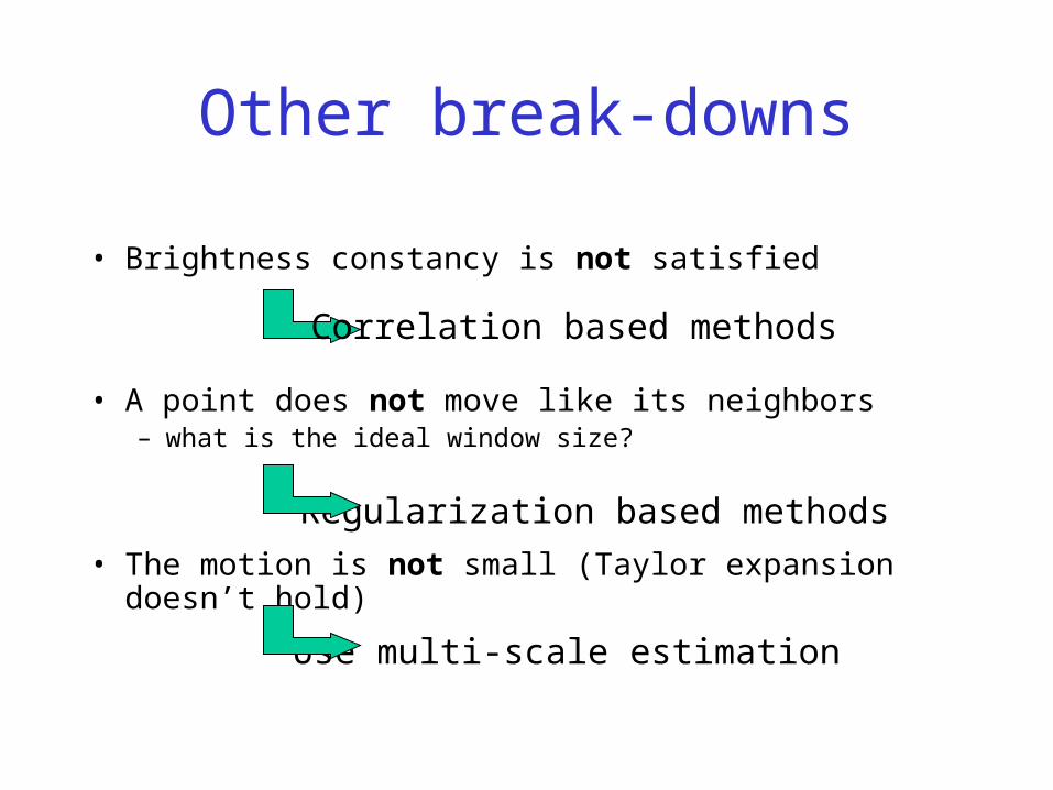
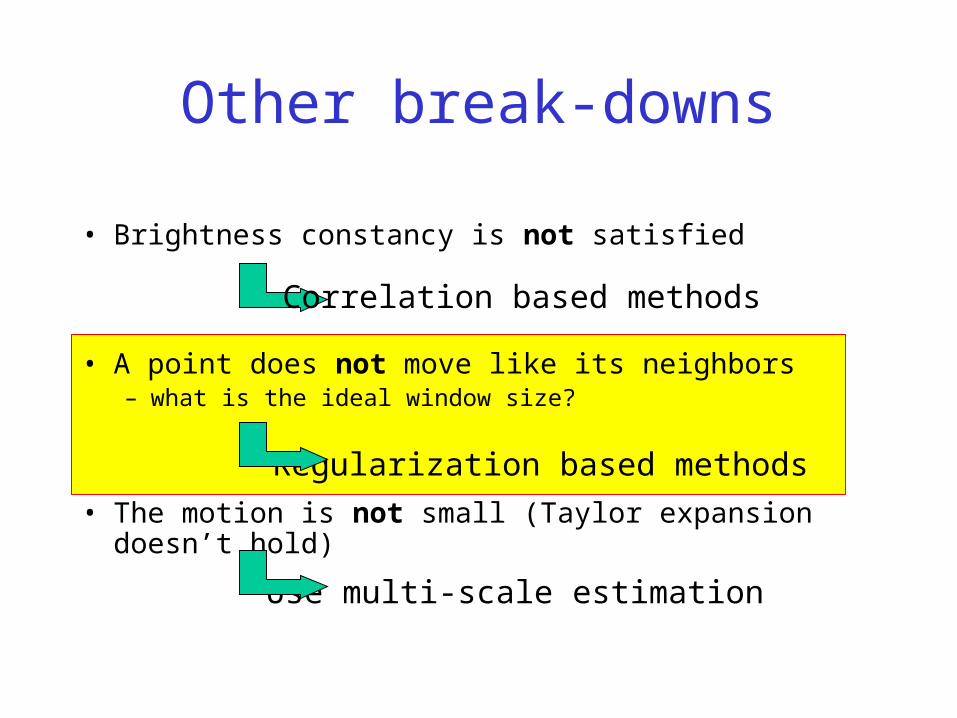
Other break-downs

• Brightness constancy is not satisfied

• A point does not move like its neighbors – what is the ideal window size?

• The motion is not small (Taylor expansion doesn’t hold)

Correlation based methods

Regularization based methods

Use multi-scale estimation

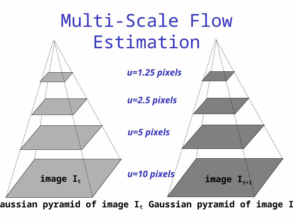
Multi-Scale Flow Estimation

image It-1 image I

Gaussian pyramid of image It Gaussian pyramid of image It+1

image It+1image Itu=10 pixels

u=5 pixels

u=2.5 pixels

u=1.25 pixels

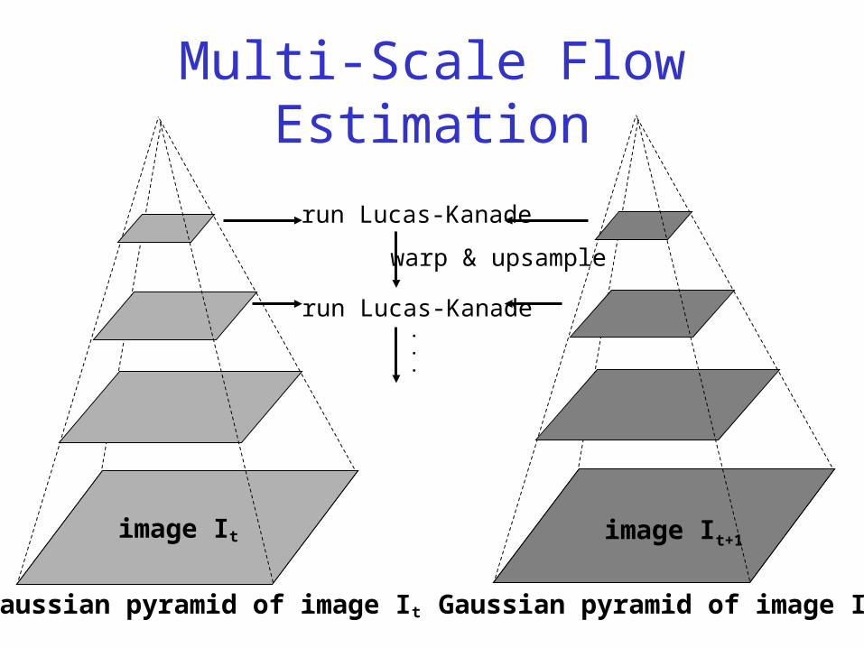
Multi-Scale Flow Estimation

image It-1 image I

Gaussian pyramid of image It Gaussian pyramid of image It+1

image It+1image It

run Lucas-Kanade

run Lucas-Kanade

warp & upsample

.

.

.

Result by: L.Zelnik-Manor, M.Machline, M.Irani

“Multi-body Segmentation: Revisiting Motion Consistency” To appear, IJCV

Examples: Motion Based Segmentation

Input Segmentation result

Result by: L.Zelnik-Manor, M.Machline, M.Irani

“Multi-body Segmentation: Revisiting Motion Consistency” To appear, IJCV

Examples: Motion Based Segmentation

Input Segmentation result

Other break-downs

• Brightness constancy is not satisfied

• A point does not move like its neighbors – what is the ideal window size?

• The motion is not small (Taylor expansion doesn’t hold)

Correlation based methods

Regularization based methods

Use multi-scale estimation

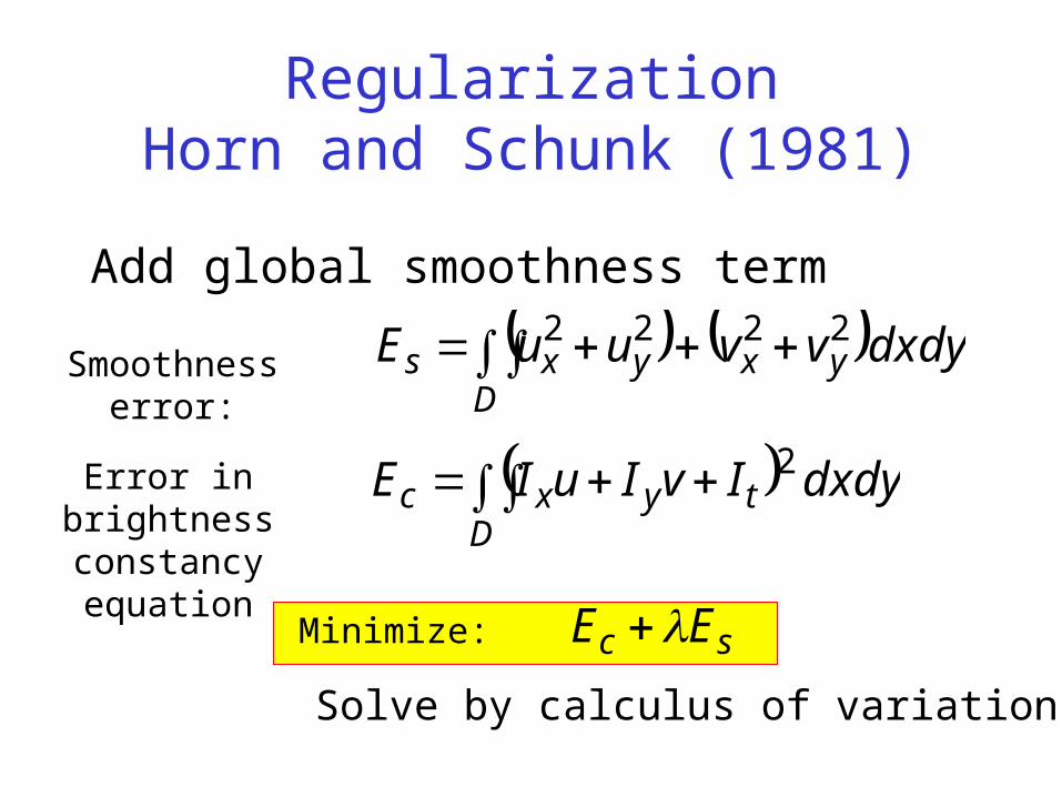
RegularizationHorn and Schunk (1981)

Add global smoothness term

dydxvvuuED

yxyxs 2222Smoothness error:

dydxIvIuIED

tyxc 2Error in brightness constancy equation

sc EE Minimize:

Solve by calculus of variations

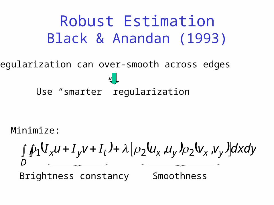
Robust EstimationBlack & Anandan (1993)

Regularization can over-smooth across edges

Use “smarter” regularization

dydxvvuuIvIuI yxyxD

tyx ,, 221

Minimize:

Brightness constancy Smoothness

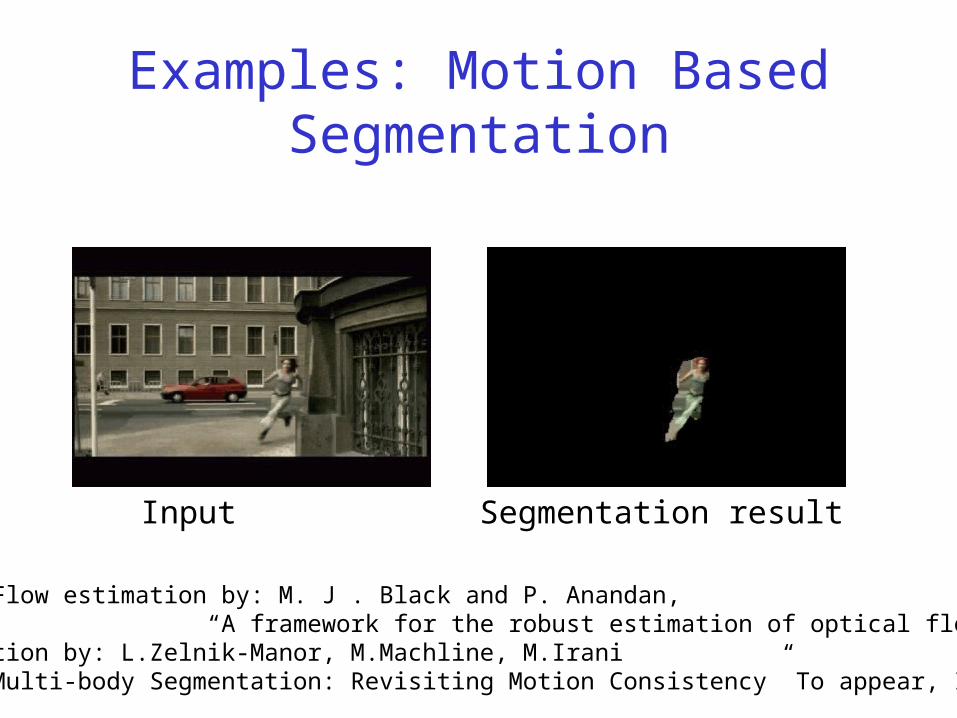
Examples: Motion Based Segmentation

•Optical Flow estimation by: M. J . Black and P. Anandan, “A framework for the robust estimation of optical flow”, ICCV’93•Segmentation by: L.Zelnik-Manor, M.Machline, M.Irani “Multi-body Segmentation: Revisiting Motion Consistency” To appear, IJCV

Input Segmentation result

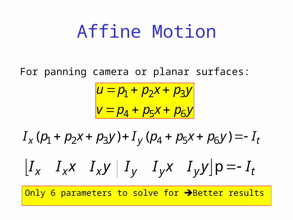
Affine Motion

For panning camera or planar surfaces:

ypxppv

ypxppu

654

321

tyx IypxppIypxppI )()( 654321

tyyyxxx IyIxIIyIxII p

Only 6 parameters to solve for Better results

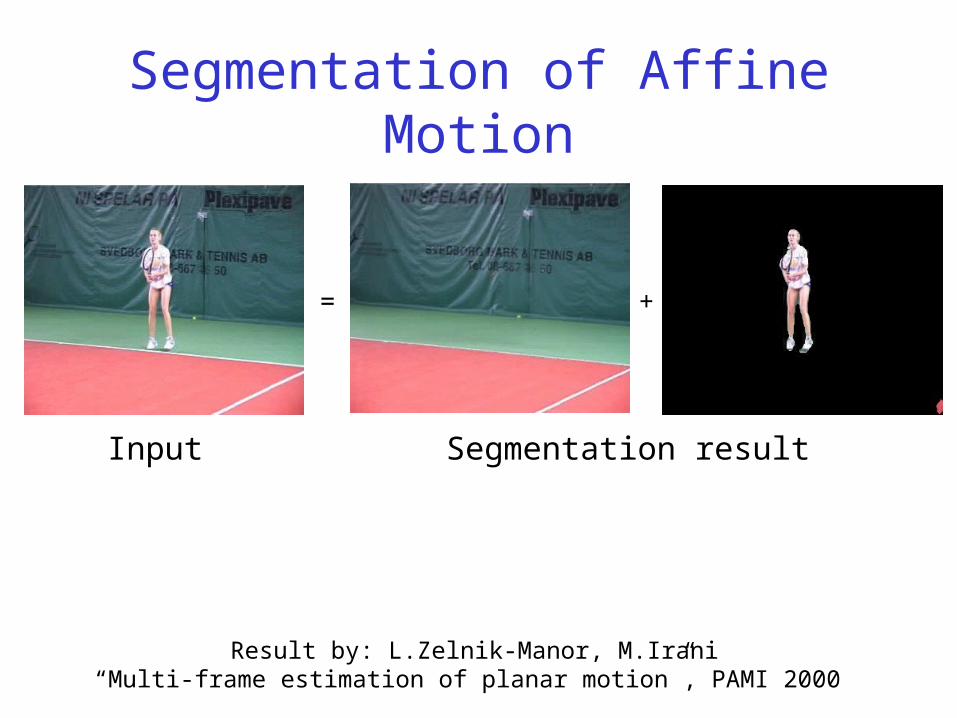
Segmentation of Affine Motion

= +

Input Segmentation result

Result by: L.Zelnik-Manor, M.Irani“Multi-frame estimation of planar motion”, PAMI 2000

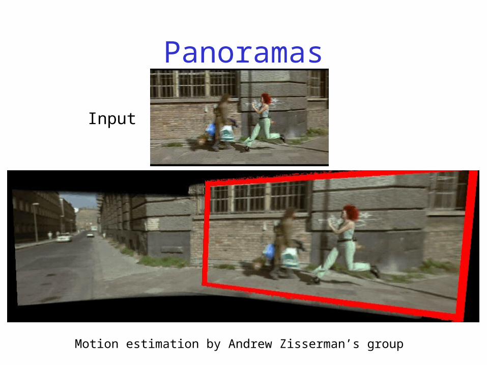
Panoramas

Motion estimation by Andrew Zisserman’s group

Input

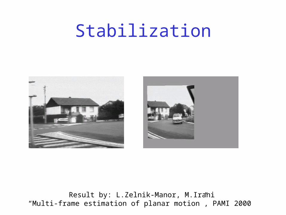
Stabilization

Result by: L.Zelnik-Manor, M.Irani“Multi-frame estimation of planar motion”, PAMI 2000

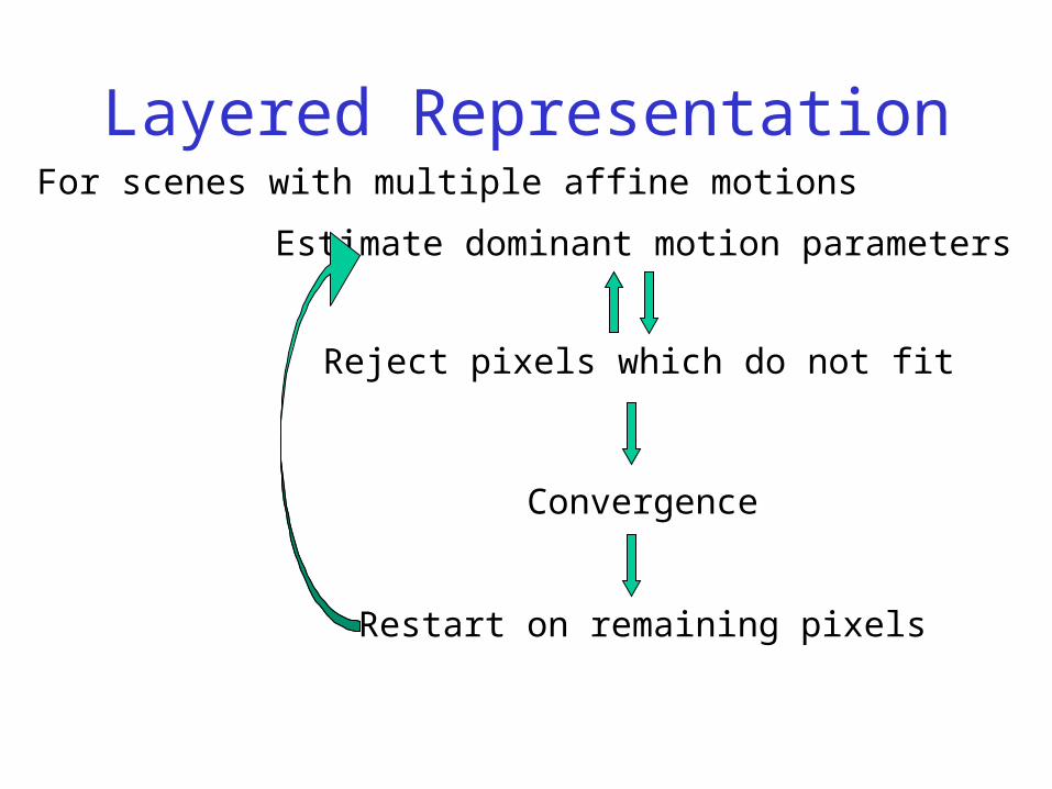
Layered Representation

Estimate dominant motion parameters

Reject pixels which do not fit

Convergence

Restart on remaining pixels

For scenes with multiple affine motions

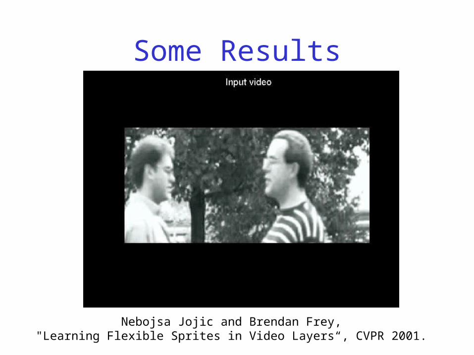
Some Results

Nebojsa Jojic and Brendan Frey, "Learning Flexible Sprites in Video Layers“, CVPR 2001.

Action Recognition

• A bit more fun

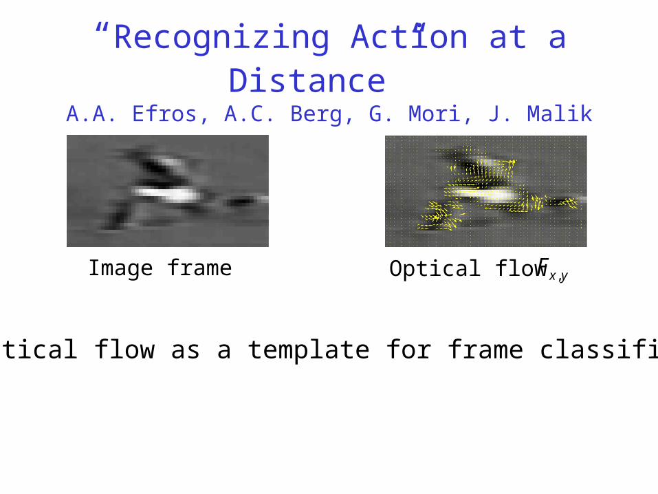
“Recognizing Action at a Distance”

A.A. Efros, A.C. Berg, G. Mori, J. Malik

Image frame Optical flow yxF ,

Use optical flow as a template for frame classification

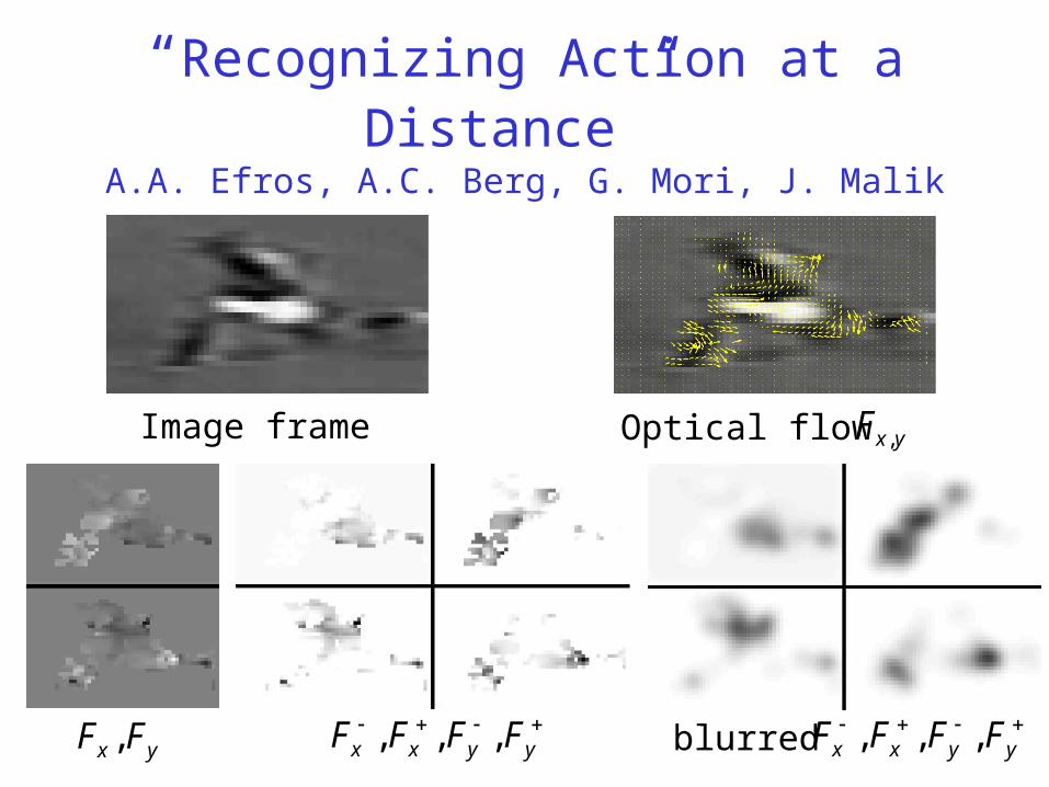
“Recognizing Action at a Distance”

A.A. Efros, A.C. Berg, G. Mori, J. Malik

Image frame Optical flow yxF ,

yx FF , yyxx FFFF ,,, blurred

yyxx FFFF ,,,

“Recognizing Action at a Distance”

A.A. Efros, A.C. Berg, G. Mori, J. Malik

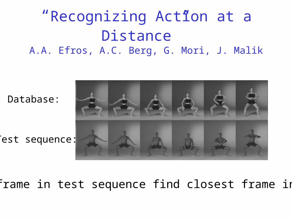
Database:

Test sequence:

For each frame in test sequence find closest frame in database

“Recognizing Action at a Distance”

A.A. Efros, A.C. Berg, G. Mori, J. Malik

•Red bars show classification results

“Recognizing Action at a Distance”

A.A. Efros, A.C. Berg, G. Mori, J. Malik

View “Greg In World Cup” video

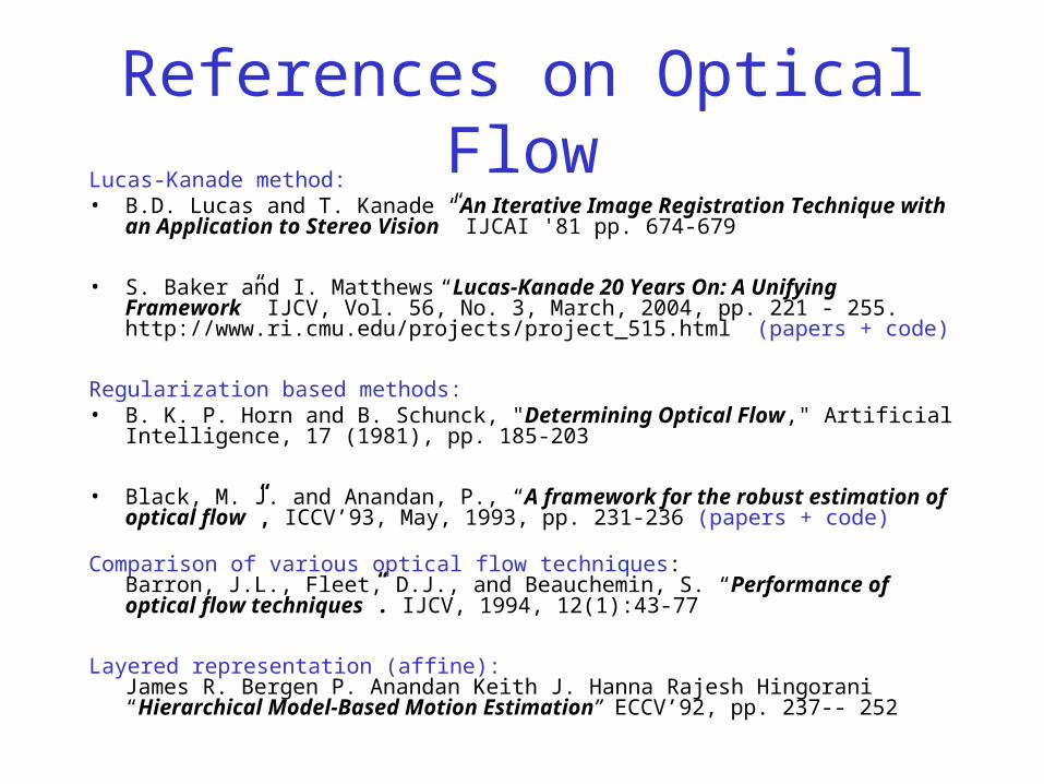
References on Optical Flow

Lucas-Kanade method:• B.D. Lucas and T. Kanade “An Iterative Image Registration Technique with an

Application to Stereo Vision” IJCAI '81 pp. 674-679

• S. Baker and I. Matthews “Lucas-Kanade 20 Years On: A Unifying Framework” IJCV, Vol. 56, No. 3, March, 2004, pp. 221 - 255.http://www.ri.cmu.edu/projects/project_515.html (papers + code)

Regularization based methods:• B. K. P. Horn and B. Schunck, "Determining Optical Flow," Artificial Intelligence, 17

(1981), pp. 185-203

• Black, M. J. and Anandan, P., “A framework for the robust estimation of optical flow”, ICCV’93, May, 1993, pp. 231-236 (papers + code)

Comparison of various optical flow techniques:Barron, J.L., Fleet, D.J., and Beauchemin, S. “Performance of optical flow techniques”. IJCV, 1994, 12(1):43-77

Layered representation (affine):James R. Bergen P. Anandan Keith J. Hanna Rajesh Hingorani “Hierarchical Model-Based Motion Estimation” ECCV’92, pp. 237-- 252  

That’s all for today